Dr. Jayaram Reddy, Centre for Molecular and computational Biology, St. Joseph’s College, Bangalore.

560027.

Measures of statistical dispersion A measure of statistical dispersion is a nonnegative real number that is zero if all

the data are the same and increases as the data become more diverse. Most measures of dispersion have the same scale as the quantity being measured.

In other words, if the measurements have units such as metres or seconds, the measure of dispersion has the same units. Such measures of dispersion include:

Standard deviation Interquartile range or Interdecile range Range Mean difference Median absolute deviation Average absolute deviation (or simply called average deviation) Distance standard deviation These are frequently used (together with scale factors) as estimators of scale

parameters, in which capacity they are called estimates of scale. Robust measures of scale are those unaffected by a small number of outliers.

All the above measures of statistical dispersion have the useful property that they are location-invariant, as well as linear in scale. So if a random variable X has a dispersion of SX then a linear transformation Y = aX + b for real a and b should have dispersion SY = |a|SX.

Other measures of dispersion are dimensionless (scale-free). In other words, they have no units even if the variable itself has units. These include:

Coefficient of variation Quartile coefficient of dispersion Relative mean difference, equal to twice the Gini coefficient There are other measures of dispersion: Variance (the square of the standard deviation) — location-invariant but not

linear in scale. Variance-to-mean ratio — mostly used for count data when the term

coefficient of dispersion is used and when this ratio is dimensionless, as count data are themselves dimensionless: otherwise this is not scale-free.

Some measures of dispersion have specialized purposes, among them the Allan variance and the Hadamard variance.

For categorical variables, it is less common to measure dispersion by a single number. See qualitative variation. One measure that does so is the discrete entropy.

Sources of statistical dispersion In the physical sciences, such variability may result from random measurement

errors: instrument measurements are often not perfectly precise, i.e., reproducible, and there is additional inter-rater variability in interpreting and reporting the measured results. One may assume that the quantity being measured is stable, and that the variation between measurements is due to observational error. A system of a large number of particles is characterized by the mean values of a relatively few number of macroscopic quantities such as temperature, energy, and density. The standard deviation is an

Dr. Jayaram Reddy, Centre for Molecular and computational Biology, St. Joseph’s College, Bangalore.

560027.

important measure in Fluctuation theory, which explains many physical phenomena, including why the sky is blue.[1]

In the biological sciences, the quantity being measured is seldom unchanging and stable, and the variation observed might additionally be intrinsic to the phenomenon: It may be due to inter-individual variability, that is, distinct members of a population differing from each other. Also, it may be due to intra-individual variability, that is, one and the same subject differing in tests taken at different times or in other differing conditions. Such types of variability are also seen in the arena of manufactured products; even there, the meticulous scientist finds variation.

In economics, finance, and other disciplines, regression analysis attempts to explain the dispersion of a dependent variable, generally measured by its variance, using one or more independent variables each of which itself has positive dispersion. The fraction of variance explained is called the coefficient of determination.

A partial ordering of dispersion A mean-preserving spread (MPS)[2] is a change from one probability distribution A

to another probability distribution B, where B is formed by spreading out one or more portions of A's probability density function while leaving the mean (the expected value) unchanged. The concept of a mean-preserving spread provides a partial ordering of probability distributions according to their dispersions: of two probability distributions, one may be ranked as having more dispersion than the other, or alternatively neither may be ranked as having more dispersion.

In probability theory and statistics, the variance is a measure of how far a set of numbers is spread out. It is one of several descriptors of a probability distribution, describing how far the numbers lie from the mean (expected value). In particular, the variance is one of the moments of a distribution. In that context, it forms part of a systematic approach to distinguishing between probability distributions. While other such approaches have been developed, those based on moments are advantageous in terms of mathematical and computational simplicity.

The variance is a parameter describing in part either the actual probability distribution of an observed population of numbers, or the theoretical probability distribution of a sample (a not-fully-observed population) of numbers. In the latter case a sample of data from such a distribution can be used to construct an estimate of its variance: in the simplest cases this estimate can be the sample variance, defined below.

Basic discussion Examples The variance of a random variable or distribution is the expectation, or mean, of

the squared deviation of that variable from its expected value or mean. Thus the variance is a measure of the amount of variation of the values of that variable, taking account of all possible values and their probabilities or weightings (not just the extremes which give the range).

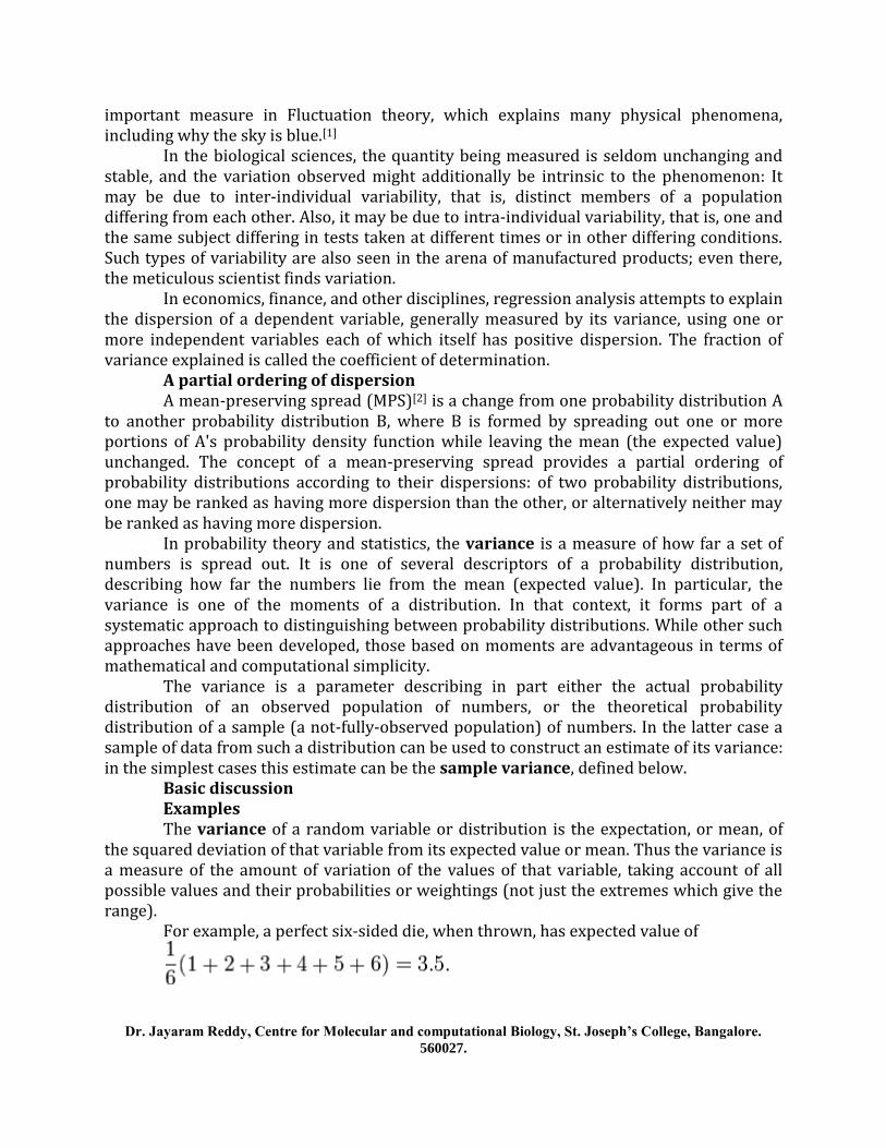
For example, a perfect six-sided die, when thrown, has expected value of

Dr. Jayaram Reddy, Centre for Molecular and computational Biology, St. Joseph’s College, Bangalore.

560027.

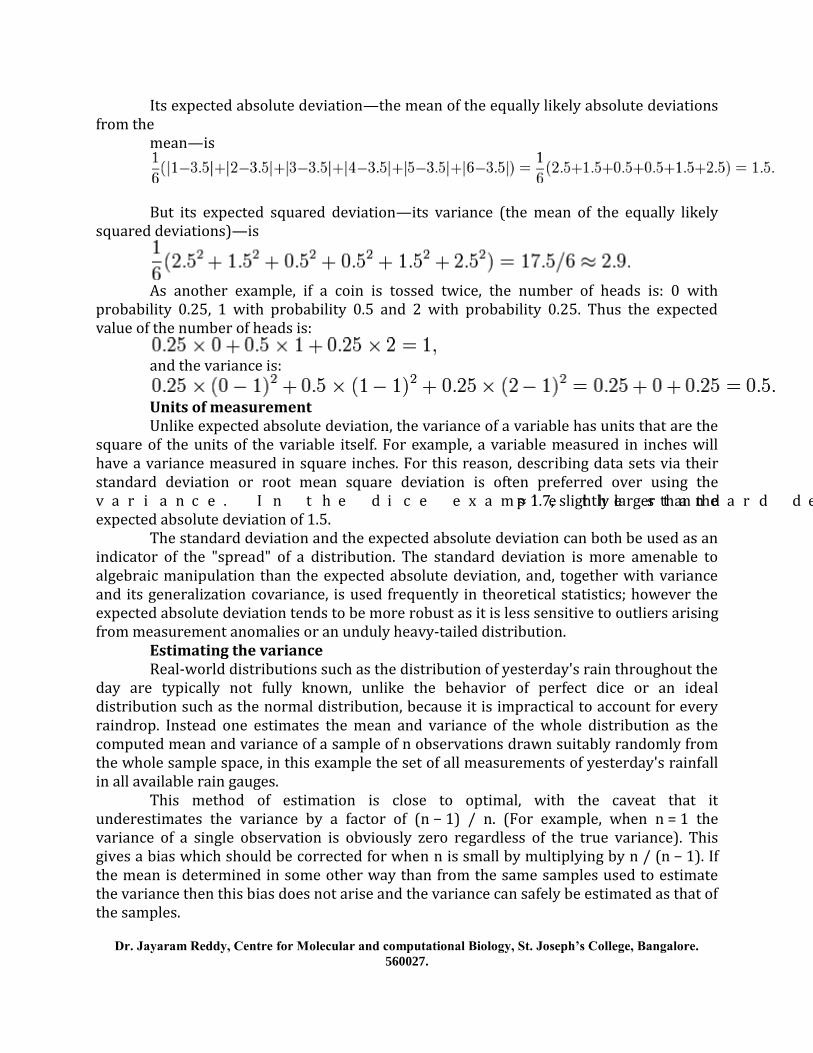
Its expected absolute deviation—the mean of the equally likely absolute deviations from the

mean—is

But its expected squared deviation—its variance (the mean of the equally likely

squared deviations)—is

As another example, if a coin is tossed twice, the number of heads is: 0 with

probability 0.25, 1 with probability 0.5 and 2 with probability 0.25. Thus the expected value of the number of heads is:

and the variance is:

Units of measurement Unlike expected absolute deviation, the variance of a variable has units that are the

square of the units of the variable itself. For example, a variable measured in inches will have a variance measured in square inches. For this reason, describing data sets via their standard deviation or root mean square deviation is often preferred over using the variance. In the dice example the standard deviation is √2.9 ≈ 1.7, slightly larger than the expected absolute deviation of 1.5.

The standard deviation and the expected absolute deviation can both be used as an indicator of the "spread" of a distribution. The standard deviation is more amenable to algebraic manipulation than the expected absolute deviation, and, together with variance and its generalization covariance, is used frequently in theoretical statistics; however the expected absolute deviation tends to be more robust as it is less sensitive to outliers arising from measurement anomalies or an unduly heavy-tailed distribution.

Estimating the variance Real-world distributions such as the distribution of yesterday's rain throughout the

day are typically not fully known, unlike the behavior of perfect dice or an ideal distribution such as the normal distribution, because it is impractical to account for every raindrop. Instead one estimates the mean and variance of the whole distribution as the computed mean and variance of a sample of n observations drawn suitably randomly from the whole sample space, in this example the set of all measurements of yesterday's rainfall in all available rain gauges.

This method of estimation is close to optimal, with the caveat that it underestimates the variance by a factor of (n − 1) / n. (For example, when n = 1 the variance of a single observation is obviously zero regardless of the true variance). This gives a bias which should be corrected for when n is small by multiplying by n / (n − 1). If the mean is determined in some other way than from the same samples used to estimate the variance then this bias does not arise and the variance can safely be estimated as that of the samples.

Dr. Jayaram Reddy, Centre for Molecular and computational Biology, St. Joseph’s College, Bangalore.

560027.

To illustrate the relation between the population variance and the sample variance, suppose that in the (not entirely observed) population of numerical values, the value 1 occurs 1/3 of the time, the value 2 occurs 1/3 of the time, and the value 4 occurs 1/3 of the time. The population mean is (1/3)[1 + 2 + 4] = 7/3. The equally likely deviations from the population mean are 1 − 7/3, 2 − 7/3, and 4 − 7/3. The population variance — the expected squared deviation from the mean 7/3 — is (1/3)[(−4/3)2 + (−1/3)2 + (5/3)2] = 14/9. Now suppose for the sake of a simple example that we take a very small sample of n = 2 observations, and consider the nine equally likely possibilities for the set of numbers within that sample: (1, 1), (1, 2), (1,4), (2, 1), (2,2), (2, 4), (4,1), (4, 2), and (4, 4). For these nine possible samples, the sample variance of the two numbers is respectively 0, 1/4, 9/4, 1/4, 0, 4/4, 9/4, 4/4, and 0. With our plan to observe two values, we could end up computing any of these sample variances (and indeed if we hypothetically could observe a pair of numbers many times, we would compute each of these sample variances 1/9 of the time). So the expected value, over all possible samples that might be drawn from the population, of the computed sample variance is (1/9)[0 + 1/4 + 9/4 + 1/4 + 0 + 4/4 + 9/4 + 4/4 + 0] = 7/9. This value of 7/9 for the expected value of our sample variance computation is a substantial underestimate of the true population variance, which we computed as 14/9, because our sample size of just two observations was so small. But if we adjust for this downward bias by multiplying our computed sample variance, whichever it may be, by n/(n − 1) = 2/(2 − 1) = 2, then our estimate of the population variance would be any one of 0, 1/2, 9/2, 1/2, 0, 4/2, 9/2, 4/2, and 0. The average of these is indeed the correct population variance of 14/9, so on average over all possible samples we would have the correct estimate of the population variance.

The variance of a real-valued random variable is its second central moment, and it also happens to be its second cumulant. Just as some distributions do not have a mean, some do not have a variance. The mean exists whenever the variance exists, but the converse is not necessarily true.

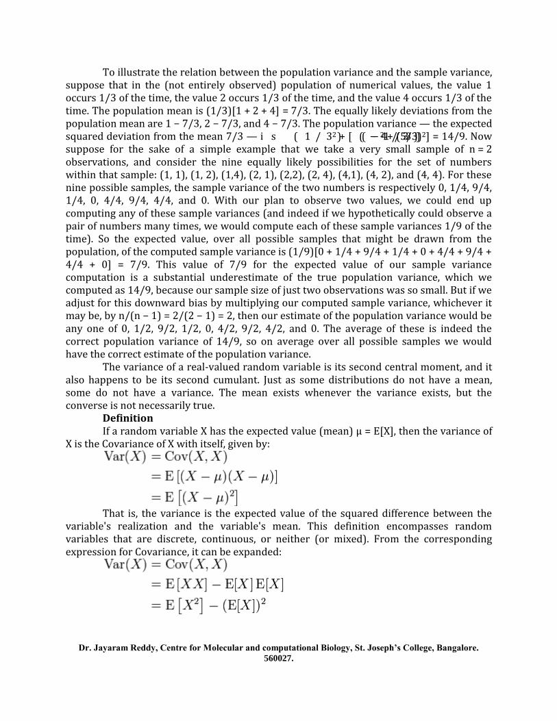
Definition If a random variable X has the expected value (mean) μ = E[X], then the variance of

X is the Covariance of X with itself, given by:

That is, the variance is the expected value of the squared difference between the

variable's realization and the variable's mean. This definition encompasses random variables that are discrete, continuous, or neither (or mixed). From the corresponding expression for Covariance, it can be expanded:

Dr. Jayaram Reddy, Centre for Molecular and computational Biology, St. Joseph’s College, Bangalore.

560027.

A mnemonic for the above expression is "mean of square minus square of mean".

The variance of random variable X is typically designated as Var(X), , or simply σ2 (pronounced "sigma squared").

Continuous random variable If the random variable X is continuous with probability density function f(x), then

the variance equals the second central moment, given by

where is the expected value,

and where the integrals are definite integrals taken for x ranging over the range

of X. If a continuous distribution does not have an expected value, as is the case for the

Cauchy distribution, it does not have a variance either. Many other distributions for which the expected value does exist also do not have a finite variance because the integral in the variance definition diverges. An example is a Pareto distribution whose index k satisfies 1 < k ≤ 2.

Discrete random variable If the random variable X is discrete with probability mass function

x1 mp1, ..., xn mpn, then

where is the expected value, i.e.

. (When such a discrete weighted variance is specified by weights whose sum is

not 1, then one divides by the sum of the weights.) That is, it is the expected value of the square of the deviation of X from its own mean. In plain language, it can be expressed as "The mean of the squares of the deviations of the data points from the average". It is thus the mean squared deviation.

Examples Exponential distribution The exponential distribution with parameter λ is a continuous distribution whose

support is the semi-infinite interval [0,∞). Its probability density function is given by:

and it has expected value μ = λ−1. Therefore the variance is equal to:

So for an exponentially distributed random variable σ2 = μ2.

Dr. Jayaram Reddy, Centre for Molecular and computational Biology, St. Joseph’s College, Bangalore.

560027.

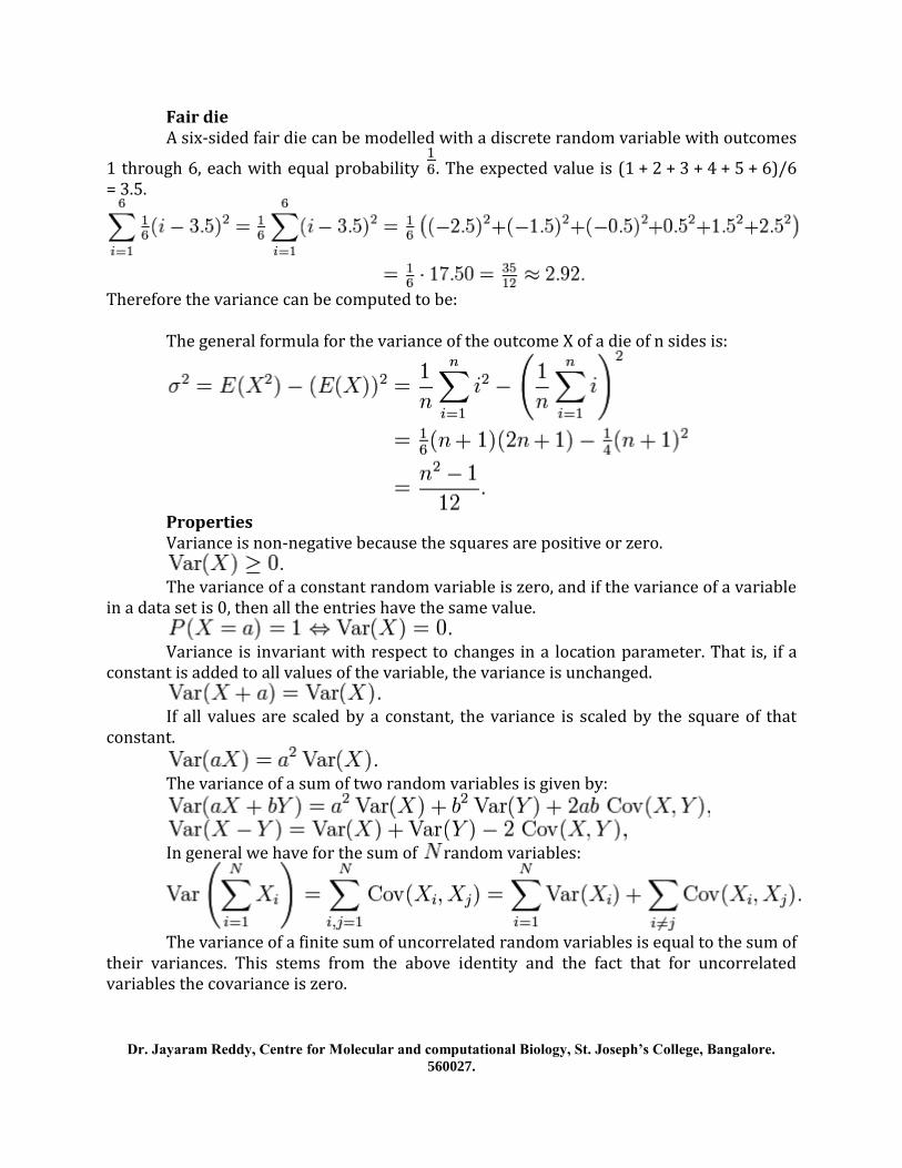
Fair die A six-sided fair die can be modelled with a discrete random variable with outcomes

1 through 6, each with equal probability . The expected value is (1 + 2 + 3 + 4 + 5 + 6)/6 = 3.5.

Therefore the variance can be computed to be: The general formula for the variance of the outcome X of a die of n sides is:

Properties Variance is non-negative because the squares are positive or zero.

The variance of a constant random variable is zero, and if the variance of a variable

in a data set is 0, then all the entries have the same value.

Variance is invariant with respect to changes in a location parameter. That is, if a

constant is added to all values of the variable, the variance is unchanged.

If all values are scaled by a constant, the variance is scaled by the square of that

constant.

The variance of a sum of two random variables is given by:

In general we have for the sum of random variables:

The variance of a finite sum of uncorrelated random variables is equal to the sum of

their variances. This stems from the above identity and the fact that for uncorrelated variables the covariance is zero.

Dr. Jayaram Reddy, Centre for Molecular and computational Biology, St. Joseph’s College, Bangalore.

560027.

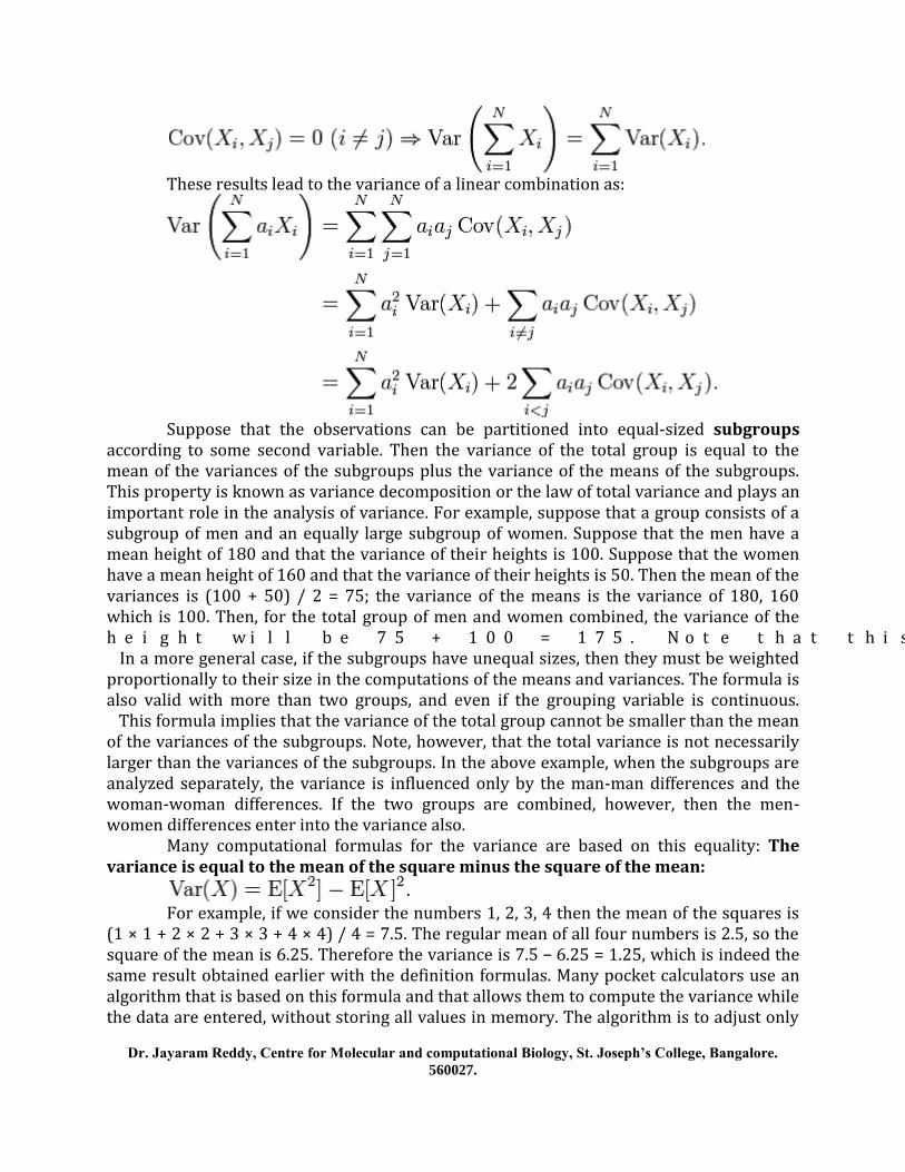
These results lead to the variance of a linear combination as:

Suppose that the observations can be partitioned into equal-sized subgroups

according to some second variable. Then the variance of the total group is equal to the mean of the variances of the subgroups plus the variance of the means of the subgroups. This property is known as variance decomposition or the law of total variance and plays an important role in the analysis of variance. For example, suppose that a group consists of a subgroup of men and an equally large subgroup of women. Suppose that the men have a mean height of 180 and that the variance of their heights is 100. Suppose that the women have a mean height of 160 and that the variance of their heights is 50. Then the mean of the variances is (100 + 50) / 2 = 75; the variance of the means is the variance of 180, 160 which is 100. Then, for the total group of men and women combined, the variance of the height will be 75 + 100 = 175. Note that this uses N for the denominator instead of N − 1. In a more general case, if the subgroups have unequal sizes, then they must be weighted proportionally to their size in the computations of the means and variances. The formula is also valid with more than two groups, and even if the grouping variable is continuous. This formula implies that the variance of the total group cannot be smaller than the mean of the variances of the subgroups. Note, however, that the total variance is not necessarily larger than the variances of the subgroups. In the above example, when the subgroups are analyzed separately, the variance is influenced only by the man-man differences and the woman-woman differences. If the two groups are combined, however, then the men-women differences enter into the variance also.

Many computational formulas for the variance are based on this equality: The variance is equal to the mean of the square minus the square of the mean:

For example, if we consider the numbers 1, 2, 3, 4 then the mean of the squares is

(1 × 1 + 2 × 2 + 3 × 3 + 4 × 4) / 4 = 7.5. The regular mean of all four numbers is 2.5, so the square of the mean is 6.25. Therefore the variance is 7.5 − 6.25 = 1.25, which is indeed the same result obtained earlier with the definition formulas. Many pocket calculators use an algorithm that is based on this formula and that allows them to compute the variance while the data are entered, without storing all values in memory. The algorithm is to adjust only

Dr. Jayaram Reddy, Centre for Molecular and computational Biology, St. Joseph’s College, Bangalore.

560027.

three variables when a new data value is entered: The number of data entered so far (n), the sum of the values so far (S), and the sum of the squared values so far (SS). For example, if the data are 1, 2, 3, 4, then after entering the first value, the algorithm would have n = 1, S = 1 and SS = 1. After entering the second value (2), it would have n = 2, S = 3 and SS = 5. When all data are entered, it would have n = 4, S = 10 and SS = 30. Next, the mean is computed as M = S / n, and finally the variance is computed as SS / n − M × M. In this example the outcome would be 30 / 4 − 2.5 × 2.5 = 7.5 − 6.25 = 1.25. If the unbiased sample estimate is to be computed, the outcome will be multiplied by n / (n − 1), which yields 1.667 in this example.

Properties, formal Sum of uncorrelated variables (Bienaymé formula) See also: Sum of normally distributed random variables One reason for the use of the variance in preference to other measures of

dispersion is that the variance of the sum (or the difference) of uncorrelated random variables is the sum of their variances:

This statement is called the Bienaymé formula.[1] and was discovered in 1853. It is

often made with the stronger condition that the variables are independent, but uncorrelatedness suffices. So if all the variables have the same variance σ2, then, since division by n is a linear transformation, this formula immediately implies that the variance of their mean is

That is, the variance of the mean decreases when n increases. This formula for the

variance of the mean is used in the definition of the standard error of the sample mean, which is used in the central limit theorem.

Product of independent variables If two variables X and Y are independent, the variance of their product is given

by[2][3]

Sum of correlated variables In general, if the variables are correlated, then the variance of their sum is the sum

of their covariances:

(Note: This by definition includes the variance of each variable, since

Cov(Xi,Xi) = Var(Xi).) Here Cov is the covariance, which is zero for independent random variables (if it

exists). The formula states that the variance of a sum is equal to the sum of all elements in

Dr. Jayaram Reddy, Centre for Molecular and computational Biology, St. Joseph’s College, Bangalore.

560027.

the covariance matrix of the components. This formula is used in the theory of Cronbach's alpha in classical test theory.

So if the variables have equal variance σ2 and the average correlation of distinct variables is ρ, then the variance of their mean is

This implies that the variance of the mean increases with the average of the

correlations. Moreover, if the variables have unit variance, for example if they are standardized, then this simplifies to

This formula is used in the Spearman–Brown prediction formula of classical test

theory. This converges to ρ if n goes to infinity, provided that the average correlation remains constant or converges too. So for the variance of the mean of standardized variables with equal correlations or converging average correlation we have

Therefore, the variance of the mean of a large number of standardized variables is

approximately equal to their average correlation. This makes clear that the sample mean of correlated variables does generally not converge to the population mean, even though the Law of large numbers states that the sample mean will converge for independent variables.

Weighted sum of variables The scaling property and the Bienaymé formula, along with this property from the

covariance page: Cov(aX, bY) = ab Cov(X, Y) jointly imply that

This implies that in a weighted sum of variables, the variable with the largest

weight will have a disproportionally large weight in the variance of the total. For example, if X and Y are uncorrelated and the weight of X is two times the weight of Y, then the weight of the variance of X will be four times the weight of the variance of Y.

The expression above can be extended to a weighted sum of multiple variables:

Decomposition The general formula for variance decomposition or the law of total variance is: If

and are two random variables and the variance of exists, then

Here, is the conditional expectation of given , and is the conditional variance of given . (A more intuitive explanation is that given a particular

value of , then follows a distribution with mean and variance .

The above formula tells how to find based on the distributions of these two quantities when is allowed to vary.) This formula is often applied in analysis of variance, where the corresponding formula is

Dr. Jayaram Reddy, Centre for Molecular and computational Biology, St. Joseph’s College, Bangalore.

560027.

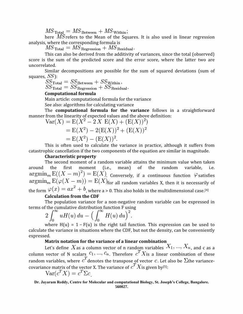
here refers to the Mean of the Squares. It is also used in linear regression

analysis, where the corresponding formula is

This can also be derived from the additivity of variances, since the total (observed)

score is the sum of the predicted score and the error score, where the latter two are uncorrelated.

Similar decompositions are possible for the sum of squared deviations (sum of squares, ):

Computational formula Main article: computational formula for the variance See also: algorithms for calculating variance The computational formula for the variance follows in a straightforward

manner from the linearity of expected values and the above definition:

This is often used to calculate the variance in practice, although it suffers from

catastrophic cancellation if the two components of the equation are similar in magnitude. Characteristic property The second moment of a random variable attains the minimum value when taken

around the first moment (i.e., mean) of the random variable, i.e.

. Conversely, if a continuous function satisfies

for all random variables X, then it is necessarily of

the form , where a > 0. This also holds in the multidimensional case.[4] Calculation from the CDF The population variance for a non-negative random variable can be expressed in

terms of the cumulative distribution function F using

where H(u) = 1 − F(u) is the right tail function. This expression can be used to

calculate the variance in situations where the CDF, but not the density, can be conveniently expressed.

Matrix notation for the variance of a linear combination

Let's define as a column vector of n random variables , and c as a

column vector of N scalars . Therefore is a linear combination of these

random variables, where denotes the transpose of vector . Let also be the variance-

covariance matrix of the vector X. The variance of is given by[5]:

.

Dr. Jayaram Reddy, Centre for Molecular and computational Biology, St. Joseph’s College, Bangalore.

560027.

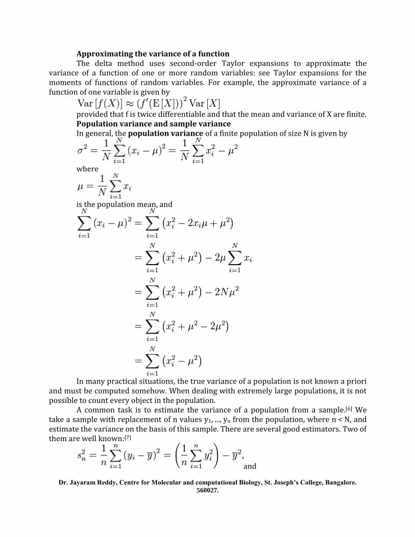
Approximating the variance of a function The delta method uses second-order Taylor expansions to approximate the

variance of a function of one or more random variables: see Taylor expansions for the moments of functions of random variables. For example, the approximate variance of a function of one variable is given by

provided that f is twice differentiable and that the mean and variance of X are finite. Population variance and sample variance In general, the population variance of a finite population of size N is given by

where

is the population mean, and

In many practical situations, the true variance of a population is not known a priori

and must be computed somehow. When dealing with extremely large populations, it is not possible to count every object in the population.

A common task is to estimate the variance of a population from a sample.[6] We take a sample with replacement of n values y1, ..., yn from the population, where n < N, and estimate the variance on the basis of this sample. There are several good estimators. Two of them are well known:[7]

and

Dr. Jayaram Reddy, Centre for Molecular and computational Biology, St. Joseph’s College, Bangalore.

560027.

The first estimator, also known as the second central moment, is called the biased

sample variance. The second estimator is called the unbiased sample variance. Either estimator may be simply referred to as the sample variance when the version can be determined by context. Here, denotes the sample mean:

The two estimators only differ slightly as can be seen, and for larger values of the

sample size n the difference is negligible. While the first one may be seen as the variance of the sample considered as a population, the second one is the unbiased estimator of the population variance, meaning that its expected value E[s2] is equal to the true variance of the sampled random variable; the use of the term n − 1 is called Bessel's correction. In particular,

while, in contrast,

The unbiased sample variance is a U-statistic for the function ƒ(x1, x2) = (x1 − x2)2/2,

meaning that it is obtained by averaging a 2-sample statistic over 2-element subsets of the population.

Distribution of the sample variance Being a function of random variables, the sample variance is itself a random

variable, and it is natural to study its distribution. In the case that yi are independent observations from a normal distribution, Cochran's theorem shows that s2 follows a scaled chi-squared distribution (see Knight 2000, proposition 2.11 [8]):

As a direct consequence, it follows that E(s2) = σ2. If the yi are independent and identically distributed, but not necessarily normally

distributed, then[citation needed]

where κ is the excess kurtosis of the distribution. If the yi are furthermore normally distributed, the variance reduces then to[9]:

Dr. Jayaram Reddy, Centre for Molecular and computational Biology, St. Joseph’s College, Bangalore.

560027.

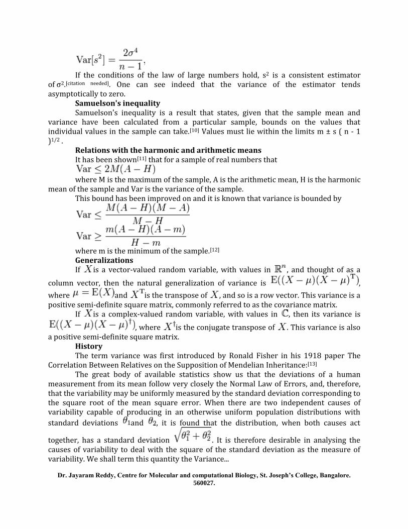
If the conditions of the law of large numbers hold, s2 is a consistent estimator

of σ2.[citation needed]. One can see indeed that the variance of the estimator tends asymptotically to zero.

Samuelson's inequality Samuelson's inequality is a result that states, given that the sample mean and

variance have been calculated from a particular sample, bounds on the values that individual values in the sample can take.[10] Values must lie within the limits m ± s ( n - 1 )1/2 .

Relations with the harmonic and arithmetic means It has been shown[11] that for a sample of real numbers that

where M is the maximum of the sample, A is the arithmetic mean, H is the harmonic

mean of the sample and Var is the variance of the sample. This bound has been improved on and it is known that variance is bounded by

where m is the minimum of the sample.[12] Generalizations If is a vector-valued random variable, with values in , and thought of as a

column vector, then the natural generalization of variance is ,

where and is the transpose of , and so is a row vector. This variance is a positive semi-definite square matrix, commonly referred to as the covariance matrix.

If is a complex-valued random variable, with values in , then its variance is

, where is the conjugate transpose of . This variance is also a positive semi-definite square matrix.

History The term variance was first introduced by Ronald Fisher in his 1918 paper The

Correlation Between Relatives on the Supposition of Mendelian Inheritance:[13] The great body of available statistics show us that the deviations of a human

measurement from its mean follow very closely the Normal Law of Errors, and, therefore, that the variability may be uniformly measured by the standard deviation corresponding to the square root of the mean square error. When there are two independent causes of variability capable of producing in an otherwise uniform population distributions with

standard deviations and , it is found that the distribution, when both causes act

together, has a standard deviation . It is therefore desirable in analysing the causes of variability to deal with the square of the standard deviation as the measure of variability. We shall term this quantity the Variance...

Dr. Jayaram Reddy, Centre for Molecular and computational Biology, St. Joseph’s College, Bangalore.

560027.

Moment of Inertia The variance of a probability distribution is analogous to the moment of inertia in

classical mechanics of a corresponding mass distribution along a line, with respect to rotation about its center of mass.[citation needed] It is because of this analogy that such things as the variance are called moments of probability distributions.[citation needed] The covariance matrix is related to the moment of inertia tensor for multivariate distributions. The moment of inertia of a cloud of n points with a covariance matrix of is given by[citation

needed]

This difference between moment of inertia in physics and in statistics is clear for

points that are gathered along a line. Suppose many points are close to the x axis and distributed along it. The covariance matrix might look like

That is, there is the most variance in the x direction. However, physicists would

consider this to have a low moment about the x axis so the moment-of-inertia tensor is

In statistics and probability theory, standard deviation (represented by the

symbol sigma, ʎ) shows how much variation or "dispersion" exists from the average (mean, or expected value). A low standard deviation indicates that the data points tend to be very close to the mean, whereas high standard deviation indicates that the data points are spread out over a large range of values.

The standard deviation of a random variable, statistical population, data set, or probability distribution is the square root of its variance. It is algebraically simpler though practically less robust than the average absolute deviation.[1][2] A useful property of standard deviation is that, unlike variance, it is expressed in the same units as the data.

In addition to expressing the variability of a population, standard deviation is commonly used to measure confidence in statistical conclusions. For example, the margin of error in polling data is determined by calculating the expected standard deviation in the results if the same poll were to be conducted multiple times. The reported margin of error is typically about twice the standard deviation – the radius of a 95 percent confidence interval. In science, researchers commonly report the standard deviation of experimental data, and only effects that fall far outside the range of standard deviation are considered statistically significant – normal random error or variation in the measurements is in this way distinguished from causal variation. Standard deviation is also important in finance, where the standard deviation on the rate of return on an investment is a measure of the volatility of the investment.

When only a sample of data from a population is available, the population standard deviation can be estimated by a modified quantity called the sample standard deviation, explained below.

Dr. Jayaram Reddy, Centre for Molecular and computational Biology, St. Joseph’s College, Bangalore.

560027.

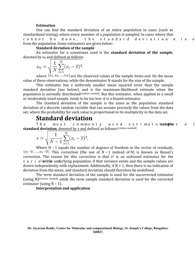
Estimation One can find the standard deviation of an entire population in cases (such as

standardized testing) where every member of a population is sampled. In cases where that cannot be done, the standard deviation σ is estimated by examining a random sample taken from the population. Some estimators are given below:

Standard deviation of the sample An estimator for σ sometimes used is the standard deviation of the sample,

denoted by sN and defined as follows.

where are the observed values of the sample items and is the mean

value of these observations, while the denominator N stands for the size of the sample. This estimator has a uniformly smaller mean squared error than the sample

standard deviation (see below), and is the maximum-likelihood estimate when the population is normally distributed[citation needed]. But this estimator, when applied to a small or moderately sized sample, tends to be too low: it is a biased estimator.

The standard deviation of the sample is the same as the population standard deviation of a discrete random variable that can assume precisely the values from the data set, where the probability for each value is proportional to its multiplicity in the data set.

Standard deviation The most commonly used estimator for σ is an adjusted version, the sample

standard deviation, denoted by s and defined as follows:[citation needed]

Where N − 1 equals the number of degrees of freedom in the vector of residuals,

. This correction (the use of N − 1 instead of N) is known as Bessel's correction. The reason for this correction is that s2 is an unbiased estimator for the variance σ2 of the underlying population, if that variance exists and the sample values are drawn independently with replacement. Additionally, if N = 1, then there is no indication of deviation from the mean, and standard deviation should therefore be undefined.

The term standard deviation of the sample is used for the uncorrected estimator (using N)[citation needed] while the term sample standard deviation is used for the corrected estimator (using N − 1).

Interpretation and application

Dr. Jayaram Reddy, Centre for Molecular and computational Biology, St. Joseph’s College, Bangalore.

560027.

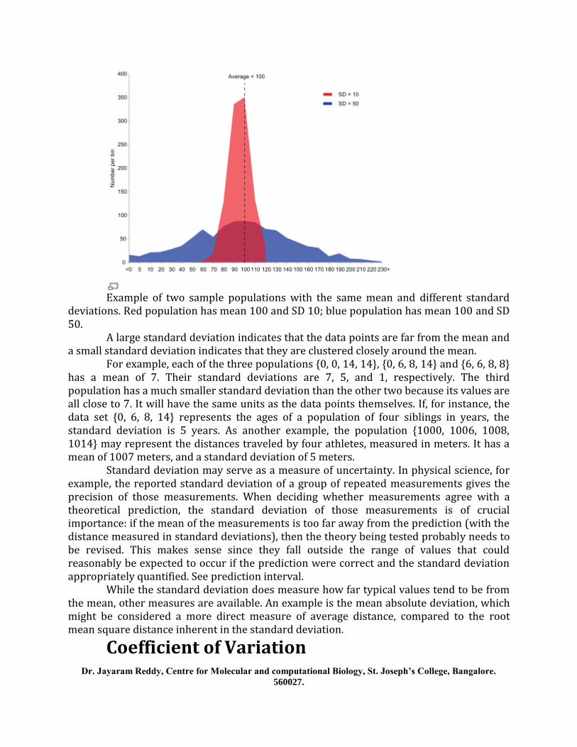
Example of two sample populations with the same mean and different standard deviations. Red population has mean 100 and SD 10; blue population has mean 100 and SD 50.

A large standard deviation indicates that the data points are far from the mean and a small standard deviation indicates that they are clustered closely around the mean.

For example, each of the three populations {0, 0, 14, 14}, {0, 6, 8, 14} and {6, 6, 8, 8} has a mean of 7. Their standard deviations are 7, 5, and 1, respectively. The third population has a much smaller standard deviation than the other two because its values are all close to 7. It will have the same units as the data points themselves. If, for instance, the data set {0, 6, 8, 14} represents the ages of a population of four siblings in years, the standard deviation is 5 years. As another example, the population {1000, 1006, 1008, 1014} may represent the distances traveled by four athletes, measured in meters. It has a mean of 1007 meters, and a standard deviation of 5 meters.

Standard deviation may serve as a measure of uncertainty. In physical science, for example, the reported standard deviation of a group of repeated measurements gives the precision of those measurements. When deciding whether measurements agree with a theoretical prediction, the standard deviation of those measurements is of crucial importance: if the mean of the measurements is too far away from the prediction (with the distance measured in standard deviations), then the theory being tested probably needs to be revised. This makes sense since they fall outside the range of values that could reasonably be expected to occur if the prediction were correct and the standard deviation appropriately quantified. See prediction interval.

While the standard deviation does measure how far typical values tend to be from the mean, other measures are available. An example is the mean absolute deviation, which might be considered a more direct measure of average distance, compared to the root mean square distance inherent in the standard deviation.

Coefficient of Variation

Dr. Jayaram Reddy, Centre for Molecular and computational Biology, St. Joseph’s College, Bangalore.

560027.

In probability theory and statistics, the coefficient of variation (CV) is a normalized measure of dispersion of a probability distribution. It is also known as unitized risk or the variation coefficient. The absolute value of the CV is sometimes known as relative standard deviation (RSD), which is expressed as a %.

Definition The coefficient of variation (CV) is defined as the ratio of the standard deviation

to the mean :

which is the inverse of the signal-to-noise ratio. It shows the extent of variability in

relation to mean of the population. The coefficient of variation should be computed only for data measured on a ratio

scale, which are measurements that can only take non-negative values. The coefficient of variation may not have any meaning for data on an interval scale.[1] For example, most temperature scales are interval scales (e.g. Celsius, Fahrenheit etc.), they can take both positive and negative values. The Kelvin scale has an absolute null value, and no negative values can naturally occur. Hence, the Kelvin scale is a ratio scale. While the standard deviation (SD) can be derived on both the Kelvin and the Celsius scale (with both leading to the same SDs), the CV is only relevant as a measure of relative variability for the Kelvin scale.

Often, laboratory values that are measured based on chromatographic methods are log-normally distributed. In this case, the CV would be constant over a large range of measurements, while SDs would vary depending on typical values that are being measured.

Estimation When only a sample of data from a population is available, the population CV can

be estimated using the ratio of the sample standard deviation to the sample mean :

But this estimator, when applied to a small or moderately sized sample, tends to be

too low: it is a biased estimator. For normally distributed data, an unbiased estimator[2] for a sample of size n is:

If it is assumed that the data are log-normally distributed, a more accurate

estimate, derived from the properties of the log-normal distribution,[3][4][5] is defined as:

where is the sample standard deviation of the data after a natural log

transformation. (In the event that measurements are recorded using any other logarithmic

base, b, their standard deviation is converted to base e using , and the

formula for remains the same.[6]) This estimate is sometimes referred to as the “geometric coefficient of variation”[7] in order to distinguish it from the simple estimate above. However, "geometric coefficient of variation" has also been defined[8] as:

Dr. Jayaram Reddy, Centre for Molecular and computational Biology, St. Joseph’s College, Bangalore.

560027.

This term was intended to be analogous to the coefficient of variation, for describing multiplicative variation in log-normal data, but this definition of GCV has no theoretical basis as an estimate of itself.

For many practical purposes (such as sample size determination and calculation of confidence intervals) it is which is of most use in the context of log-normally distributed data. If necessary, this can be derived from an estimate of or GCV by inverting the corresponding formula.

Comparison to standard deviation Advantages The coefficient of variation is useful because the standard deviation of data must

always be understood in the context of the mean of the data. Instead, the actual value of the CV is independent of the unit in which the measurement has been taken, so it is a dimensionless number. For comparison between data sets with different units or widely different means, one should use the coefficient of variation instead of the standard deviation.

Disadvantages When the mean value is close to zero, the coefficient of variation will

approach infinity and is hence sensitive to small changes in the mean. This is often the case if the values do not originate from a ratio scale.

Unlike the standard deviation, it cannot be used directly to construct confidence intervals for the mean.

Applications The coefficient of variation is also common in applied probability fields such as

renewal theory, queueing theory, and reliability theory. In these fields, the exponential distribution is often more important than the normal distribution. The standard deviation of an exponential distribution is equal to its mean, so its coefficient of variation is equal to 1. Distributions with CV < 1 (such as an Erlang distribution) are considered low-variance, while those with CV > 1 (such as a hyper-exponential distribution) are considered high-variance. Some formulas in these fields are expressed using the squared coefficient of variation, often abbreviated SCV. In modeling, a variation of the CV is the CV(RMSD). Essentially the CV(RMSD) replaces the standard deviation term with the Root Mean Square Deviation (RMSD).