Max–Planck–Institut fur BiogeochemieMax Planck Institute for Biogeochemistry

MPI fur Biogeochemie · Postfach 10 01 64 · 07745 Jena, Germany

Dr. Jens-Arne SubkeAssociate EditorBiogeosciences

Dr. Carlos A. SierraResearch group leaderTel.: +49-(0)3641-57-6133csierra@bgc-jena.mpg.de

29th December 2020

Dear Jens,

We are submitting here a new revised version of our manuscript with changes basedon your suggestions. In particular, we fixed typos and clarified references to theAppendices, and added extra information regarding the supplementary material.You can see the new changes in the attached file with track-changes markup.

We hope the manuscript is now ready for publication. Thanks for your editorialwork,

Best regards,

Carlos A. Sierra, PhDOn behalf of all authors

Max-Planck-Institut furBiogeochemieHans-Knoll-Straße 1007745 JenaGermany

Tel.: + 49-(0) 3641 / 57 – 6110Fax.: + 49-(0) 3641 / 57 – 6110http:// www.bgc-jena.mpg.de

DirektoriumSusan Trumbore

Markus Reichstein (Managing Dir.)Sonke Zaehle

ID-Nr. DE 129517720

The Climate Benefit of Carbon SequestrationCarlos A. Sierra1, Susan E. Crow2, Martin Heimann1,3, Holger Metzler1, and Ernst-Detlef Schulze1

1Max Planck Institute for Biogeochemistry, 07745 Jena, Germany2University of Hawaii Manoa, Honolulu, HI 96822, USA3University of Helsinki, 00560 Helsinki, Finland

Correspondence: Carlos A. Sierra (csierra@bgc-jena.mpg.de)

Abstract. Ecosystems play a fundamental role in climate change mitigation by photosynthetically fixing carbon from the

atmosphere and storing it for a period of time in organic matter. Although climate impacts of carbon emissions by sources

can be quantified by global warming potentials, the appropriate formal metrics to assess climate benefits of carbon removals

by sinks are unclear. We introduce here the Climate Benefit of Sequestration (CBS), a metric that quantifies the radiative

effect of fixing carbon dioxide from the atmosphere and retaining it for a period of time in an ecosystem before releasing5

it back as the result of respiratory processes and disturbances. In order to quantify CBS, we present a formal definition of

carbon sequestration (CS) as the integral of an amount of carbon removed from the atmosphere stored over the time horizon

it remains within an ecosystem. Both metrics incorporate the separate effects of i) inputs (amount of atmospheric carbon

removal), and ii) transit time (time of carbon retention) on carbon sinks, which can vary largely for different ecosystems or

forms of management. These metrics can be useful for comparing the climate impacts of carbon removals by different sinks10

over specific time horizons, to assess the climate impacts of ecosystem management, and to obtain direct quantifications of

climate impacts as the net effect of carbon emissions by sources versus removals by sinks.

1 Introduction

Terrestrial ecosystems exchange carbon with the atmosphere at globally significant quantities, thereby influencing Earth’s

climate and potentially mitigating warming caused by increasing concentrations of CO2 in the atmosphere. Carbon fixed during15

the process of photosynthesis remains stored in the terrestrial biosphere over a range of timescales, from days to millennia;

timescales of relevance for affecting the concentration of greenhouse gases in the atmosphere (Archer et al., 2009; IPCC, 2014;

Joos et al., 2013). During the time carbon is stored in the terrestrial biosphere, it is removed from the radiative forcing effect

that occurs in the atmosphere; thus, it is of scientific and policy relevance to understand the timescale of carbon storage in

ecosystems; i.e., for how long newly fixed carbon is retained in an ecosystem before it is released back to the atmosphere.20

Timescales of element cycling and storage are unambiguously characterized by the concepts of system age and transit

time (Bolin and Rodhe, 1973; Rodhe, 2000; Rasmussen et al., 2016; Sierra et al., 2017; Lu et al., 2018). In a system of

multiple interconnected compartments, system age characterizes the time that the mass of an element observed in the system

has remained there since its entry. Transit time characterizes the time that it takes element masses to traverse the entire system,

from the time of entry until they are released back to the external environment (Sierra et al., 2017). Both metrics are excellent25

1

system-level diagnostics of the dynamics and timescales of ecosystem processes. Because system age and transit time both can

be reported as mass- or probability distributions, they provide different information about an ecosystem over a wide range in

the time domain.

System age and transit time are closely related to the complexity of the ecosystem and its process rates, which are affected

by the environment (Luo et al., 2017; Rasmussen et al., 2016; Sierra et al., 2017; Lu et al., 2018). Mean system ages of carbon30

are consistently greater than mean transit time (Lu et al., 2018; Sierra et al., 2018b), suggesting that once a mass of carbon

enters an ecosystem, a large proportion gets quickly released back to the atmosphere, but a small proportion remains for very

long times. Furthermore, differences in transit times across ecosystems suggest that not all carbon sequestered in the terrestrial

biosphere spends the same amount of time stored; e.g., one unit of photosynthesized carbon is returned back to the atmosphere

faster in a tropical than in a boreal forest (Lu et al., 2018). Therefore, not all carbon drawn down from the atmosphere should35

be treated equally for the purpose of quantifying the climate mitigation potential of sequestering carbon in ecosystems as it is

currently recommended in accounting methodologies (IPCC, 2006).

Global warming potentials (GWPs, see definition in section 2) quantify the radiative effects of greenhouse gases emitted

to the atmosphere (Fig. 1), but do not consider the avoided radiative effect of storing carbon in ecosystems (Neubauer and

Megonigal, 2015). GWPs are computed using the age distribution of CO2 and other greenhouse gases in the atmosphere40

(Rodhe, 1990; Joos et al., 2013), but do not consider age or transit times of carbon in ecosystems in the case of sequestration.

Transit time distributions, in particular, can better inform us about the time newly sequestered carbon will be removed from

radiative effects in the atmosphere.

For more comprehensive accounting of the contribution of carbon sequestration to climate change mitigation, it is necessary

to quantify the avoided warming effects of sequestered carbon in ecosystems over the timescale the carbon is stored. The45

GWP metric is inappropriate to quantify avoided warming potential as a result of sequestration. A metric that can capture this

avoided warming effect could have applications for 1) comparing different carbon sequestration activities considering the time

carbon is stored in ecosystems, and 2) providing better accounting methods for the effect of removals by sinks in climate policy.

Currently, the Intergovernmental Panel on Climate Change (IPCC) recommends countries and project developers to report only

emissions by sources and removals by sinks of greenhouse gases (GHGs), treating all removals equally in terms of their fate50

(IPCC, 2006).

Problems with applying GWPs to compute climate benefits of sequestering carbon in ecosystems are well documented

(Moura Costa and Wilson, 2000; Fearnside et al., 2000; Brandão et al., 2013; Neubauer and Megonigal, 2015). Several ap-

proaches have been proposed to deal with the issue of timescales (Brandão et al., 2013), many of which deal with time as some

form of delay in emissions. However, to our knowledge, no solution proposed thus far explicitly accounts for the time carbon55

is sequestered in ecosystems, from the time of photosynthetic carbon fixation until it is returned back to the atmosphere by

autotrophic and heterotrophic respiration, and fires.

Therefore, the main objective of this manuscript is to introduce a metric to assess the climate benefits of carbon sequestration

while accounting for the time carbon is stored in ecosystems. We first present the theoretical framework for the development

2

of the metric, then provide simple examples for its computation and discuss potential applications for ecosystem management60

and for climate change mitigation.

2 Theoretical framework

2.1 Absolute Global Warming Potential AWGP

The direction of carbon flow, into or out of ecosystems, is of fundamental importance to understand and quantify their contri-

bution to climate change mitigation. The absolute global warming potential (AGWP) of carbon dioxide quantifies the radiative65

effects of a unit of CO2 emitted to the atmosphere during its life time; in the direction land→ atmosphere. It is expressed as

(Lashof and Ahuja, 1990; Rodhe, 1990)

AGWP(T,t0) =

t0+T∫

t0

kCO2(t)Ma(t)dt (1)

where kCO2(t) is the radiative efficiency or greenhouse effect of one unit of CO2 (in mole or mass) in the atmosphere at time

t, and Ma(t) is the amount of gas present in the atmosphere at time t (Rodhe, 1990; Joos et al., 2013). The AGWP quantifies70

the amount of warming produced by CO2 while it stays in the atmosphere since the time the gas is emitted at time t0 over a

time horizon T . The function Ma(t) quantifies the fate of the emitted carbon in the atmosphere and can be written in general

form as

Ma(t) = ha(t− t0)Ma(t0) +

t∫

t0

ha(t− τ)Q(τ)dτ, (2)

where ha(t− t0) is the impulse response function of atmospheric CO2 released into the atmosphere; Ma(t0) is the content of75

atmospheric CO2 at time t0, and Q(τ) is the perturbation of new incoming carbon to the atmosphere between t0 and t.

For a pulse, or instantaneous emission of CO2, Ma(t0) = E0, and

Ma(t) = ha(t− t0)E0, (3)

assuming no additional carbon enters the atmosphere after the pulse. If the pulse is equivalent to 1 kg or mole of CO2, then

E0 = 1 and Ma(t) = ha(t− t0). For a pulse emission of any arbitrary size, and assuming constant radiative efficiency (see80

details about this assumption in section 2.2),

AGWP(T,E0, t0) = kCO2E0

t0+T∫

t0

ha(t− t0)dt. (4)

The AGWP can be computed for any other greenhouse gas using their respective radiative efficiencies and fate in the

atmosphere (impulse response function). To compare different gases, the Global Warming Potential (GWP) is defined as the

3

AGWP of a particular gas divided by the AGWP of CO2 (Shine et al., 1990; Lashof and Ahuja, 1990). Our interest in this85

manuscript is on carbon fixation and respiration in the form CO2, therefore we primarily concentrate here on AGWP.

The impulse response function ha(t−t0) plays a central role within the AGWP framework. The function encodes information

about the fate of a gas once it enters the atmosphere and determines for how long the gas will remain. Therefore, it can be

interpreted as a density distribution for the the transit time of a gas, since the time of emission until it is removed by natural

sinks (e.g. CO2) or by chemical reactions (e.g. CH4).90

The function typically is assumed to be static, i.e. the time at which the gas enters the atmosphere is not relevant, only the

time it remains there (t−t0). However, this function can be time-dependent, expressing different shapes depending on the time

the gas enters the atmosphere, i.e. ha(t0, t− t0). For example, when natural sinks saturate, faster accumulation of CO2 and

longer transit times of carbon in the atmosphere would be observed (Metzler et al., 2018). In this situation, the specific time

of an emission would lead to different response functions in the atmosphere. Because current research on impulse response95

functions primarily considers the static time-independent case (see Millar et al., 2017, for an exception), we will consider only

the static case for the remainder of this manuscript.

2.2 The radiative efficiency of CO2 and its impulse response function

The radiative efficiency of CO2 is a function of the concentration of this gas and the concentration of other gases in the

atmosphere with overlapping absorption bands (Lashof and Ahuja, 1990; Shine et al., 1990). Therefore, kCO2changes as the100

concentration of GHGs change in the atmosphere. For most applications however, the radiative efficiency of CO2 has been

assumed constant in the limit of a small perturbation at a specific background concentration (Lashof and Ahuja, 1990; Shine

et al., 1990; Joos et al., 2013; Myhre et al., 2013).

Here, we use a constant value of kCO2 = 6.48× 10−12 W m−2 MgC−1 based on results reported by Joos et al. (2013) for

an atmospheric background of 389 ppm (∼ present day). This radiative efficiency represents the change in radiative forcing105

caused by a change of 1 Mg of carbon in the atmosphere in the form of CO2 in units of rate of energy transfer (Watt) per square

meter of surface.

Joos et al. (2013) have also derived impulse response functions (IRFs) of CO2 in the atmosphere using coupled carbon-

climate models that include multiple feedbacks among Earth system processes. One function was obtained by emitting a pulse

of 100 GtC to a ‘pre-industrial’ atmosphere with a background concentration of 280 ppm (PI100 function from here on), and110

another function was obtained by emitting 100 GtC to a ‘present day’ atmosphere with a background of 389 ppm (PD100 from

here on). The functions they report are averages from the numerical output of multiple models fitted to a sum of exponential

functions that include an intercept term. This intercept implies that a proportion of the added CO2 never leaves from the

atmosphere-ocean-terrestrial system to long-term geological reservoirs. Following Millar et al. (2017), we added a timescale

of 1 million years that corresponds to the intercept term in the IRFs. The addition of this timescale has no effect on the results115

presented here, which are focused on much shorter timescales, but they avoid the mathematical problem that the integrals of

the original functions go to infinity with time (Lashof and Ahuja, 1990; Millar et al., 2017).

4

2.3 Carbon sequestration CS, and the climate benefit of carbon sequestration CBS

GWPs are useful to quantify the climate impacts of increasing or reducing emissions of GHGs to the atmosphere. However, it

is also necessary to quantify the climate benefits of carbon flows in the opposite direction, atmosphere→ land. Furthermore, it120

is also important to quantify not only how much and how fast carbon enters ecosystems, but also for how long the carbon stays

(Körner, 2017).

Carbon taken up from the atmosphere through the process of photosynthesis is stored in multiple ecosystem reservoirs for a

particular amount of time. Carbon sequestration can be defined as the process of capture and long-term storage of CO2 (Sedjo

and Sohngen, 2012). We define here carbon sequestration CS over a time horizon T as125

CS(T,S0, t0) :=

t0+T∫

t0

Ms(t− t0)dt, (5)

where Ms(t− t0) represents the fate of a certain amount of carbon S0 taken up by the sequestering system at a time t0. Notice

that this definition of carbon sequestration is very similar to that of AGWP for an emission, with the exception that the radiative

efficiency term is omitted.

To obtain the fate of sequestered carbon over time, we represent carbon cycling and storage in ecosystems using the theory130

of compartmental dynamical systems (Luo et al., 2017; Sierra et al., 2018a). In their most general form, we can write carbon

cycle models as

dx(t)

dt= x(t) = u(x,t) + B(x,t)x, (6)

where x(t) ∈ Rn is a vector of n ecosystem carbon pools, u(x,t) ∈ Rn is a time-dependent vector-valued function of carbon

inputs to the system, and B(x,t) ∈ Rn×n is a time-dependent compartmental matrix. The latter two terms can depend on the135

vector of states, in which case the compartmental system is considered nonlinear. In case the input vector and the compartmental

matrix have fixed coefficients (no time-dependencies), the system is considered autonomous, and non-autonomous otherwise

(Sierra et al., 2018a). This distinction of models with respect to linearity and time-dependencies (autonomy) is fundamental to

distinguish important properties of models. For instance, models expressed as autonomous linear systems have a steady-state

solution given by x∗ =−B−1u, where x∗ is a vector of steady-state contents for all ecosystem pools. Non-autonomous models140

have no steady-state solution.

The fate of the fixed carbon for the general nonlinear non-autonomous case can be obtained as

Ms(t− t0) = ‖Φ(t, t0)β(t0)S0‖, (7)

where β(t0)S0 = u(t0), and β(t0) is an n-dimension vector representing the partitioning of the total sequestered carbon

among n ecosystem carbon pools (Ceballos-Núñez et al., 2020). The n×n matrix Φ(t, t0) is the state transition operator,145

which represents the dynamics of how carbon moves in a system of multiple interconnected compartments (see details in

appendix::::::::Appendix

::B). Throughout this document, we use the symbol ‖ ‖ to denote the 1-norm of a vector, i.e. the sum of the

absolute values of all elements in a vector.

5

Because ecosystems and most reservoirs are open systems, the sequestered carbon S0 returns back to the atmosphere, mostly

as CO2 due to ecosystem respiration and fires. Carbon release r(t) from ecosystems can be obtained according to150

r(t) =−1ᵀB(t)Φ(t, t0)β(t0)S0, (8)

where 1ᵀ is the transpose of the n-dimensional vector containing only 1s. The state-transition matrix captures the entire fate

and dynamics of the sequestered carbon, from the time it enters t0 until release at any t.

The link between the time it takes sequestered carbon S0 to appear in the release flux r(t) is established by the concept of

transit time (Metzler et al., 2018). In particular, we define the forward transit time (FTT) as the age that fixed carbon will have155

at the time it is released back to the atmosphere, or, how long a mass fixed now will stay in the system. The backward transit

time (BTT) is defined as the age of the carbon in the output flux since the time it was fixed, or, how long the mas leaving the

system now had stayed. This implies that

r(t) = pBTT(t− t0, t) = pFTT(t− t0, t0), (9)

where pBTT(t− t0, t) is the backward transit time distribution of carbon leaving the system at time t with an age t− t0, while160

pFTT(t− t0, t0) is the forward transit time distribution of carbon entering the system at time t0 and leaving with an age t− t0.

For systems in equilibrium, both quantities are equal (Metzler et al., 2018). For systems not in equilibrium, semi-explicit

formulas for their distributions are given in the appendix::::::::Appendix

::B.

For the atmosphere, carbon sequestration is a form of ‘negative emission’, and we can represent its fate in the atmosphere as

165

M ′a(t) =−ha(t− t0)S0 +

t∫

t0

ha(t− τ)r(τ)dτ, (10)

where the prime symbol represents a perturbed atmosphere as an effect of sequestration. The first term in the rhs represents

the response of the atmosphere to an instantaneous sequestration S0 at t0, and the second term represents the perturbation

in the atmosphere of the carbon returning back from the terrestrial biosphere. Notice that the integral in this equation can be

written as a convolution (ha ? r)(t) between the impulse response function of atmospheric CO2 and the carbon returning from170

ecosystems to the atmosphere.

We define now the climate benefit of sequestration for a pulse of CO2 into an ecosystem as

CBS(T,S0, t0) :=

t0+T∫

t0

kCO2M′a(t)dt,

=−kCO2

t0+T∫

t0

(ha(t− t0)S0− (ha ? r)(t)) dt.

(11)

This metric integrates over a time horizon T the radiative effect avoided by sequestration of an amount of carbon S0 taken up at

time t0 by an ecosystem. It captures the timescale at which the carbon is stored and gradually returns back to the atmosphere. It175

6

can also be interpreted as the atmospheric response to carbon sequestration in the form of a negative emission of CO2 during a

time horizon of interest. It relies on knowledge of the atmospheric response to perturbations in the form of an impulse response

function, and the transit time of carbon in an ecosystem.

2.4 Ecosystems in equilibrium: the linear, steady-state case

The computation of CS and CBS is simplified for systems in equilibrium. For linear systems at steady-state, the time at which180

the carbon enters the ecosystem is irrelevant (Kloeden and Rasmussen, 2011; Rasmussen et al., 2016); one only needs to know

for how long the carbon has been in the system to predict how much of it remains. Mathematically, this implies

Φ(t, t0) = ea·B for all t0 ≤ t and a= t− t0. (12)

Therefore, for linear systems at steady state, we have the special cases

Ms(a) = ‖ea·Bu‖, (13)185

and

Ms1(a) =

∥∥∥∥ea·Bu

‖u‖

∥∥∥∥ , (14)

where Ms1 represents the fate of one unit of fixed carbon, which can also be interpreted as the proportion of carbon remaining

after the time of fixation.

The amount of released carbon returning to the atmosphere is therefore190

r(a) =−1ᵀBea·Bu, (15)

which for one unit of fixed carbon is equal to the transit time density distribution f(τ) of a linear system (Metzler and Sierra, 2018, see also appendix)

:::::::::::::::::::::::::::::::::::::::(Metzler and Sierra, 2018, see also Appendix B)

r1(a) =−1ᵀBea·Bu

‖u‖ . (16)

where r1(a) = f(τ), with mean (expected value) transit time given by195

E(τ) =−1ᵀB−1u

‖u‖ =‖x∗‖‖u‖ . (17)

We can now derive the steady-state expression of CS as

CS(T ) =

T∫

0

‖ea·Bu‖ da. (18)

Furthermore, it is possible to find a closed-form expression for this integral

CS(T ) = ‖B−1(eT ·B− I

)u‖, (19)200

7

where I ∈ Rn×n is the identity matrix. Similarly, for one unit of carbon entering a steady-state system at any time, we define

CS1 as

CS1(T ) =

T∫

0

∥∥∥∥ea·Bu

‖u‖

∥∥∥∥ da, (20)

which by integration gives

CS1(T ) =

∥∥∥∥B−1(eT ·B− I

) u

‖u‖

∥∥∥∥ . (21)205

These steady-state expressions can be very useful to compare different systems or changes to a particular system if the

steady-state assumption is justified. Furthermore, it can be shown that in the long term, as the time horizon T goes to infinity

(∞), the term (eT ·B− I) converges to −I, and therefore equation (19) converges to the expression

limT→∞

CS(T ) = ‖x∗‖, (22)

which means that the total amount of carbon at steady-state is equal to the long-term carbon sequestration of an instantaneous210

amount of fixed carbon at an arbitrary time.

Similarly, for one unit of carbon entering a system at steady-state, the long-term CS1 from equation (21) can be obtained

simply as

limT→∞

CS1(T ) = E(τ), (23)

by using the definition of mean transit time of equation (17). This means that long-term sequestration of one unit of CO2215

converges to the mean transit time of carbon in an ecosystem.

2.5 Dynamic ecosystems out of equilibrium: the continuous sequestration and emissions case

In addition of considering isolated pulses of emissions E0 or sequestrations S0, we can also consider permanently ongoing

emissions e : t 7→ E(t) and sequestration s : t 7→ S(t), respectively. Hence,

CS(T,s, t0) :=

t0+T∫

t0

Ms(t)dt, (24)220

where

Ms(t) =

t∫

t0

‖Φ(t,τ)β(τ)s(τ)‖dτ. (25)

Here s(τ) is a scalar flux of sequestration at time τ . This leads to

r(t) =−1ᵀB(t)

t∫

t0

Φ(t,τ)β(τ)s(τ)dτ. (26)

8

The fate of sequestered carbon, for the atmosphere in the form of a balance between simultaneous sequestration and return225

of carbon, can now be obtained as

M ′a(t) =−t∫

t0

ha(t− τ)s(τ)dτ +

t∫

t0

ha(t− τ)r(τ)dτ

=−t∫

t0

ha(t− τ) [s(τ)− r(τ)] dτ

=−(ha ? (s− r))(t).

(27)

We can now define the climate benefit of sequestration for a dynamic ecosystem with continuous sequestration and respiration

as

CBS(T,s, t0) :=

t0+T∫

t0

kCO2M ′a(t)dt,

=−kCO2

t0+T∫

t0

(ha ? (s− r))(t)dt.

(28)230

This expression of CBS accounts for the dynamic behavior of inputs and outputs of carbon in ecosystems, and can be used

to represent time-dependencies resulting from environmental changes, disturbances, or produced by emission scenarios or

scheduled management activities. This time-dependent CBS is computed for a time horizon T starting at any initial time t0.

In other words, it can be used to analyze specific time windows of interest, accounting for the fate of all carbon sequestered

during specific time intervals.235

3 Example 1: CS and CBS for linear systems in equilibrium

3.1 The fate of a pulse of inputs through the system

A simple ecosystem carbon model, the Terrestrial Ecosystem Model (TECO), will now demonstrate an application of the

theory to compute CS and CBS assuming a linear system at steady-state (i.e., in equilibrium). We used a modified version of

the TECO model, orginally described by Weng and Luo (2011) with parameter values obtained through data assimilation using240

observations from the Duke forest in North Carolina, USA. It contains eight main compartments: foliage x1, woody biomass

x2, fine roots x3, metabolic litter x4, structural litter x5, fast soil organic matter (SOM) x6, slow SOM x7, and passive SOM

x8 (Figure 2). The model represents the dynamics of carbon at a temperate forest dominated by loblolly pine. We chose this

model due to its simplicity and tractability, but the framework presented in section 2 can be applied to more complex models

and for other ecosystems (see supplementary material:::::::reference

:::in

::::Code

::::::::::Availability

:::::section

:for an example with a nonlinear245

model). In addition to its simplicity and tractability, there are two advantages of using this model over others: 1) it provides

reasonable predictions of net ecosystem carbon fluxes and biometric pool data (Weng and Luo, 2011), 2) it is commonly used

9

to express complex ecosystem-level concepts such as the matrix generalization of carbon cycle models, their traceability, and

transient behavior (e.g. Luo and Weng, 2011; Luo et al., 2012; Xia et al., 2013; Luo et al., 2017; Sierra, 2019).

The model is commonly expressed as250

dX(t)

dt= bU(t) + ξ(t)ACX(t), (29)

where X is a vector of ecosystem carbon pools, C is a diagonal matrix with cycling rates for each pool, A is a matrix of transfer

coefficients among pools, and b is a vector of allocation coefficients to plant parts. We modified the entries of matrix A to

allow autotrophic respiration to be computed from the vegetation pools, and not from the GPP flux as in the original model (see

details in the appendix::::::::Appendix

::C). The function U(t) determines the carbon inputs to the system as gross primary production255

(GPP), and ξ(t) is a time-dependent function that modifies ecosystem cycling rates according to changes in the environment.

For this steady state example, we assume constant inputs (U(t) = U ) and constant rates (ξ(t) = 1). Furthermore, defining

B := AC, and u := bU , we can write this model as a linear, autonomous compartmental system of the form

x= u+ Bx, (30)

with values for B and u as described in appendix::::::::Appendix C.260

The fate of a pulse of carbon input entering the ecosystem at an arbitrary time when the system is in equilibrium can

be obtained by applying equations (13) and (14) (Figure 3). Carbon enters the ecosystem through foliage, wood, and fine

root pools. A large proportion of this carbon is quickly transferred from these pools to the fine and metabolic litter pools.

Subsequently, the carbon moves to the SOM pools with important respiration losses during these transfers. Most carbon is

returned back to the atmosphere with a mean transit time of 30.4 yr for the whole system. Half of the sequestered carbon is265

returned back to the atmosphere in 7.6 yr, and 95% in 124 yr.

Ecosystem-level CS, i.e., the area under the curve of the amount of remaining carbon over time (area under dotted line in

Fig 3a), increases towards an asymptote as the time horizon of integration increases (Figure 4a). Here, CS is reported in units

of MgC ha−1 yr, because this is the amount of carbon retained in organic matter over a fixed time horizon. For relevant time

horizons of 50, 100, 500, and 1000 yr, CS was 233.51, 317.68, 371.64, and 373.42 MgC ha−1 yr, respectively. In the long-term270

(i.e., as the time horizon goes to infinity), CS converges to the steady-state carbon stock predicted by the model of 373.67 MgC

ha−1.

A similar computation can be made for one unit of fixed carbon (CS1). In this case CS1 was 18.98, 25.83, 30.21, and 30.36

yr for time horizons of 50, 100, 500, and 1000 yr, respectively. In the long-term, CS1 converges to the mean transit time of

carbon, 30.4 yr (Figure 4b).275

Due to sequestration at t0, the CBS shows a rapid negative increase in radiative forcing, which decreases as the time horizon

increases due to the return of carbon to the atmosphere as an effect of respiration (Figure 4c). The shape of the curve however,

depends strongly on the IRF for atmospheric CO2. CBS is larger over the long-term (> 200 yr) for the present day (PD100)

curve proposed by Joos et al. (2013) than for the pre-industrial curve (PI100). During the preindustrial period, perturbations

of CO2 in the atmosphere are lower than in the present day period due to higher uptake of carbon from the oceans and the280

10

land biosphere (Joos et al., 2013). Therefore, the benefits of carbon sequestration are larger under present day conditions

based on these IRF curves. Impulse response functions depend strongly on the magnitude and timing of the pulse (Joos et al.,

2013; Millar et al., 2017). Therefore, estimates of climate impacts of emissions (AGWP, Figure 5) and climate benefits of

sequestration (CBS, Figure 4c,d) depend strongly on the choice of the IRF. For the purpose of this manuscript, we will use the

present day curve (PD100) from here on.285

Because AGWP and CBS are based on similar concepts and share similar units, it becomes possible to directly compare one

another (Figure 6) and obtain an estimate of the climate impact of emissions versus sequestration. This can be done either as

the ratio of the absolute value of CBS to AGWP, i.e. | CBS | /AGWP (unitless); or as the net radiative balance CBS+AGWP

(W m−2 yr). It is possible to compute these relations using the CBS for one unit of sequestered carbon, which provides a

direct estimate of the impact of one unit of sequestration versus one unit of emission; or corresponding to the amount of GPP290

sequestered in one year (12.3 MgC ha−1 yr−1 for Duke forest).

In our example, the emission of 1 MgC to the atmosphere has a predominant warming effect that cannot be compensated

by the sequestration of 1 MgC at the Duke forest (Figure 6). However, the sequestration of the equivalent of GPP in one year

can have a significant climate benefit compared to the emission of 1MgC, depending on the time horizon of analysis. When

one integrates in time horizons lower than 200 years, CBS outweighs AGWP in this example. However, because the lifetime295

of an emission of CO2 is much longer in the atmosphere than the transit time of carbon through a forest ecosystem, AGWP

outweighs CBS on longer timescales.

The time of integration in the computation of GWP has been a heavily debated topic in the past, and this is related to the

topic of ‘permanence’ of sequestration in carbon accounting and climate policy (Moura Costa and Wilson, 2000; Noble et al.,

2000; Sedjo and Sohngen, 2012). One problem in these previous debates is that the timescale of carbon in ecosystems was300

not considered explicitly while the timescale of carbon in the atmosphere was. With the approach proposed here, both are

explicitly taken into account, and can better inform management and policy debates about sequestration of carbon in natural

and man-made sinks.

3.2 Carbon management to maximize the climate benefit of carbon sequestration

In the context of climate change mitigation, management of ecosystems may be oriented to increase carbon sequestration305

and its climate benefit. In the recent past, scientists and policy makers have advocated increasing the amount of inputs to

ecosystems as an effective form of carbon management (e.g. Silver et al., 2000; Grace, 2004; Lal, 2004; Chabbi et al., 2017;

Minasny et al., 2017). Although increases in carbon inputs can increase the amount of stored carbon in an ecosystem with

related climate benefits, it does not necessarily increase the amount of time the sequestered carbon will stay in the system.

Therefore, strategies that focus on increasing carbon inputs alone, do not take full advantage of the potential of ecosystems to310

mitigate climate change.

11

We can conceptualize any management activity that increases or reduces carbon inputs to an ecosystem by a factor γ, so the

new inputs are given by the product γ u. For example, if we increase carbon inputs to an ecosystem by 10%, γ = 1.1. Increasing

carbon inputs by a proportion γ > 1, increases carbon storage at steady state by an equal proportion since

−B−1 (γ u) =γ (−B−1u),

=γ x∗.(31)315

Similarly, a decrease in carbon inputs by a proportion γ < 1, decreases steady-state carbon storage by an equal proportion.

However, the time carbon requires to travel through the ecosystem is still the same since the transit time does not change, as

we can see from the mean transit time expression

−1ᵀB−1γ u

‖γ u‖ = E(τ). (32)

Both the transit time distribution (eq. B4 and 16) and the mean transit time (eq. 17) only take into account the proportional320

distribution of the carbon inputs to the different pools (u/‖u‖), but not the total amount of inputs. Therefore, a unit of carbon

that enters an ecosystem stays there for the same amount of time independent of how much carbon is entering the system.

Although these results only apply to linear systems at steady-state, they provide some intuition about what might be the case

in systems out of equilibrium.

Carbon management can also be oriented to modify process rates in ecosystems as encoded in the matrix B. A proportional325

decrease in process rates by a factor ξ < 1, not only increases carbon storage as

−(ξB)−1u=1

ξ(−B−1u),

=x∗

ξ,

(33)

it also increases the mean transit time as

−1ᵀ (ξB)−1u

‖u‖ =E(τ)

ξ. (34)

A proportional change in the oposite direction (ξ > 1) causes the opposite effect, a proportional increase in process rates330

decreases carbon storage and decreases mean transit time.

Based on these results, it is now clear that carbon management to increase carbon inputs alone can only increase CS, but not

CS1; i.e. the new carbon inputs have a sequestration benefit only through increase of carbon storage, but not through a longer

transit time in ecosystems. Management to decrease process rates on the contrary, can increase both CS and CS1 because the

new carbon entering the system stays there for longer.335

We can see these effects of carbon management on CS by running simulations using the TECO model at steady-state (Figure

7). Now, we modified carbon inputs and process rates by either increasing them by 10 and 50% (γ, ξ = 1.1, 1.5), or decreasing

them by 10 and 50% (γ, ξ = 0.9, 0.5). The simulations showed that increasing or decreasing carbon inputs increase or decrease

12

CS for any time horizon (Figure 7a), but it does not modify the behavior of one unit of sequestered carbon (CS1) (Figure 7b).

On the contrary, decreasing or increasing process rates increase or decrease both CS (Figure 7c) and CS1 (Figure 7d).340

The resultant effects of changes in management of inputs or process rates on CBS can differ substantially. Increases or

decreases of carbon inputs have similar proportional effects on CBS, but differences in processes rates are not equally propor-

tional. While an increase in inputs by 50% would increase CBS by 50%, a decrease in process rates by 50% would have an

increase in CBS by more than 100% for time horizons longer than 300 years (Figure 8). Similarly, while a decrease in inputs

by 50% would reduce CBS by 50%, an increase in process rates by 50% would decrease CBS by only ∼40%.345

These results show that management of transit time, e.g. by decreasing process rates, may lead to stronger climate benefits

than managing carbon inputs alone. Furthermore, one could think about optimization scenarios in which both inputs and transit

times are managed to achieve larger climate benefits given certain constraints. The concept of CBS is thus a useful mathematical

framework to formally pose such an optimization problem.

We can also use these results to infer differences in CS and CBS for different ecosystem types. Without management,350

we would expect large variability of CS and CBS in the terrestrial biosphere. Inputs and process rates vary considerably for

terrestrial ecosystems as previously reported in other studies. For instance, gross primary productivity can range between

about 1 to > 30 MgC ha−1 yr−1, from high to low latitude ecosystems (Jung et al., 2020). Based on simulations from the

CABLE model, Lu et al. (2018) found a rage:::::range of mean transit times between 13 to 341 yr, from low to high latitude

ecosystems. These large ranges of variability for GPP and mean transit time suggest that CS and CBS may vary among355

ecosystem:::::::::ecosystems by large proportions (> 20 times larger or smaller depending on the ecosystems being compared).

4 Example 2: CS and CBS for dynamic systems out of equilibrium

4.1 Pulses entering at different times and experiencing different environments

The steady-state examples above are useful to gain some intuition about potential long-term patterns in CS and CBS, but for

real-world applications it is necessary to consider systems out of equilibrium and driven by specific time-dependent signals.360

We will consider now the case of the temperate ecosystem of our previous example driven by increases in atmospheric CO2

concentrations that lead to higher photosynthetic uptake, and increasing temperatures that lead to faster cycling rates. We will

thus consider a non-autonomous version of the TECO model that follows the general form

x(t) = γ(t) ·u+ ξ(t) ·B ·x(t), (35)

where the time-dependent function γ(t) incorporates the effects of temperature and atmospheric CO2 on primary production,365

and the function ξ(t) incorporates the effects of temperature on respiration rates. Specific shapes for these functions were

taken from Rasmussen et al. (2016), and are described in detail in appendix:::::::Appendix

:C. When applied to the CASA model in

Rasmussen et al. (2016), these functions predicted an increase in primary production and an increase in process rates, which

resulted in a decrease in transit times over a simulation of 600 years.

13

We used the same simulation setup here starting from an empty system (x(0) = 0), and obtained similar results in terms of370

primary production and transit times as in Rasmussen et al. (2016). We used these simulation results to compute CS and CBS

for carbon entering the ecosystem at different times during the simulation window. In particular, we considered the case of

the amount of carbon sequestered at years 100 and 300 after the start of the simulation; i.e. we considered the cases t0 = 100

and t0 = 300 (Figure 9a) and computed the fate of this carbon (Ms(t, t0,u0)), its carbon sequestration (CS(T,u0, t0)) and the

climate benefit of sequestration (CBS(T,u0, t0)) for different time horizons T .375

Although more carbon enters the ecosystem at simulation year 300 than at year 100 due to the CO2 fertilization effect, it is

lost much faster because of higher temperatures that result in faster transit times for simulation times above 300 years (Figure

9a). The slower transit times experienced by the carbon that enters at year 100 due to lower temperature results then in much

higher values of CS for time horizons T > 100 yr (Figure 9c). Similarly for CBS, where differences are evident much earlier,

for time horizons T > 50 yr (Figure 9d).380

This simple example highlights the importance of time-dependent transit times in determining CS and CBS. If changes in

climate lead to faster carbon processing rates, we would thus expect carbon to transit faster through the ecosystem, returning

faster to the atmosphere, and therefore with lower values for carbon sequestration and its climate benefit.

4.2 Continuous inputs into a changing environment

In the previous example, we considered the case of two single pulses entering the ecosystem at different times under changing385

environmental conditions during a simulation. A consolidated view can be obtained by taking all single pulses and integrate

them continuously in time to compute CS and CBS using equations (24) and (28), respectively. In this case, CS increases

monotonically, and CBS decreases monotonically with time horizon (Figure 10, continuous black lines), which is somewhat

obvious because as the ecosystem accumulates carbon, more of it is retained in the ecosystem and is isolated from atmospheric

radiative effects. However, this simulation only considers carbon that enters the ecosystem from the beginning of the simulation390

until the end of the time horizon, from t0 to t0 +T . An important aspect to consider is the role of carbon already present in the

ecosystem at t0.

We will consider now the case of continuous sequestration and release of carbon with differences in the initial conditions in

the simulation, which can vary according to land use changes. For example, when changing land use from agriculture to forest,

or from natural forest to plantation, there are carbon legacies that have an influence on future carbon trajectories (Harmon et al.,395

1990; Janisch and Harmon, 2002; Sierra et al., 2012). These carbon legacies are usually dead biomass and detritus, which cause

ecosystems to lose carbon via decomposition before photosynthesis from new biomass compensates for the losses. In these

initial stages of recovery, ecosystems are usually net carbon sources, but they still may store more carbon than an ecosystem

developing from bare ground.

The CS and CBS concepts can be very useful to compare contrasting trajectories of ecosystem development and assess their400

role in terms of carbon sequestration alone and their climate impact. For this purpose, we performed an additional simulation in

which at the starting time there is no living biomass, but the detritus pools and the SOM pools are 1.5 and 1.0 times as large as

in the equilibrium case, respectively (x(0) = 149.04 MgC ha−1). In this simulation, the ecosystem losses a significant amount

14

of carbon in the early stages of development and respiration is much larger than primary production (r(t)> u(t)) (Fig. 10a,

dashed magenta line). Because soils are already close to an equilibrium value, the ecosystem has already a large amount of405

carbon stored, therefore in the computation of the fate of carbonMs(t, t0) there is already a larger amount of carbon to consider,

which causes CS to be larger for the land-use-change case than for the bare ground case (Figure 10c). On the contrary, because

there are more emissions from the ecosystem in early development stages, CBS is lower for the land-use-change case than for

the bare ground case (Figure 10d).

These contrasting results between CS and CBS for the continuous case with contrasting initial conditions, can be very410

useful to address debates and controversies about the role of land use change and baselines in carbon accounting. The results

show that carbon sequestration can still be high in ecosystems where emission fluxes are large, but climate impacts can differ

significantly. By using two different metrics, these two different aspects of carbon sequestration can be discussed separately.

5 Discussion

The metrics introduced here, carbon sequestration (CS) and the climate benefit of sequestration (CBS), integrate both the415

amount of carbon entering an ecosystem and the time it is stored there and thus avoiding radiative effects in the atmosphere.

Disproportionate attention is given to quantifying sources and sinks of carbon in ongoing debates about the role of ecosystems

in climate change mitigation, with much less attention to the fate of carbon once it enters an ecosystem. The time carbon

remains in an ecosystem, encapsulated in the concept of transit time, is critical for climate change mitigation because during

this time carbon is removed from radiative effects in the atmosphere.420

The CS and CBS concepts unify atmospheric and ecosystem approaches to quantifying the greenhouse effect. The CBS

concept builds on that of absolute global warming potential (AGWP) of a greenhouse gas. The main difference is that CBS

quantifies avoided warming during the time carbon is stored in an ecosystem, while AGWP quantifies potential warming when

the carbon enters the atmosphere. Both metrics rely on the quantification of the fate of carbon (or other GHGs for AGWP) once

it enters the particular system. For atmospheric systems, a significant amount of work has been done in determining the fate425

of GHGs once they enter the atmosphere after emissions (e.g. Rodhe, 1990; O’Neill et al., 1994; Prather, 1996; Archer et al.,

2009; Joos et al., 2013). For terrestrial ecosystems however, robust methods to quantify the fate of carbon as it flows through

terrestrial system components have been developed only recently (Rasmussen et al., 2016; Metzler and Sierra, 2018; Metzler

et al., 2018).

Global warming potential (GWP), or the climate impact of an emission of a certain gas in relation to the impact of an emission430

of CO2, is often used to assess climate impacts of actions, e.g., avoided deforestation, land use change, and even enhanced

carbon sequestration. However, this metric has two limitations when applied to carbon sequestration and in comparison to

the combined use of CBS and AGWP we advocate here: 1) it only quantifies the climate effects of emissions but not of

sequestration, and treats all fixed carbon equally independent of its transit time in the ecosystem, 2) it is a relative measure

with respect to the emission of CO2. GWPs are commonly reported in units of CO2-equivalents, which only address indirectly435

15

the effect of a gas in producing warming. In contrast, CBS quantifies the effects of avoided warming in units of W m−2 over

the period of time carbon is retained.

Other concepts have been proposed in the past to account for the temporary nature of carbon sequestration (see review

by Brandão et al., 2013, and references therein), with special interest in accounting for credits in carbon markets. In fact,

‘ton-year’ accounting methods (Noble et al., 2000) resemble our definition of carbon sequestration; however, none of these440

previous concepts explicitly considers the time carbon is retained in the ecosystem. Instead, these approaches relate carbon

sequestration to delay in fossil fuel emissions (Fearnside et al., 2000), or as the equivalence of the amount of carbon storage

to AGWP (Moura Costa and Wilson, 2000). The concepts of sustained global warming potential SGWP and sustained global

cooling potential SGCP proposed by Neubauer and Megonigal (2015) are notable exceptions. The CBS concept captures some

of the ideas of the SGCP concept, but differs in some fundamental assumptions related to the interpretation of the impulse445

response functions, the treatment of time-dependent fluxes and rates, and reporting. While SGCP reports values in reference

to CO2 as is commonly done for GWP, we report CBS for individual gases as it is done for AGWP. Appendix A elaborates on

other aspects of the SGWP and SGCP concepts.

The concept of CBS improves our ability to address some of the existing debates about the role of ecosystems in mitigating

climate change and enhances our potential to provide decision-support. In combination with quantifications of AGWP, CBS450

provides the net climate effect of an ecosystem or some management. For example, CBS can be used to better understand

the climate impacts of storing carbon in long-term reservoirs such as soils and wood products, and the climate benefits of

increasing the transit time in these systems. CBS can be used to better quantify the climate benefits of using biofuels as fossil

fuel substitution by computing the CBS of the whole bioenergy production system and adding the negative AGWP attributed

to the avoided emission. Similarly, it can be incorporated in assessments of sequestration in industrial systems with associated455

carbon capture and storage.

Carbon management of ecosystems can maximize CS and/or CBS by not only increasing carbon inputs, but also by increas-

ing the transit time of carbon. There are many ways in which the transit time of carbon can be increased; for instance, by

increasing transfers of carbon to slow cycling pools such as the case of increasing wood harvest allocation to long-duration

products (Schulze et al., 2019), or addition of biochar to soils, or by reducing cycling rates of organic matter such as the case460

of soil flipping (Schiedung et al., 2019). Independently of the management activity, CS and CBS can be powerful metrics to

quantify their climate benefits, make comparisons among them, and compare against baselines or no management scenarios.

The examples we provided in this manuscript illustrate the use and interpretation of CS and CBS metrics under the as-

sumptions of linearity, steady-state, or time-dependencies in carbon cycle dynamics with subsequent consequences for carbon

sequestration and its climate benefits. The computation of the CBS relies on a model, which can be as simple as a one-pool465

model or a state-of-the-science land surface model. The TECO model is an excellent tool to illustrate ecosystem-level concepts

because of its simplicity and tractability, but other models with more accurate parameterizations and including more processes

should be considered for practical applications. The formulas and formal theory developed in Section 2 are general enough to

deal with the non-steady-state case as well as with models with nonlinear interactions among state variables. In the supplemen-

16

tary material, we provide an example:in

:::the

:::::form

::of

:a:::::::

Jupyter::::::::Notebook

:to compute CS and CBS for a nonlinear model

:::(see470

::::Code

::::::::::Availability

::::::section

:::for

::::::details).

The concepts of CS and CBS present improvements to the current guidelines for carbon inventories that treat all carbon

removals by sinks equally (IPCC, 2006) by explicitly considering the transit time of carbon in ecosystems. Therefore, these new

concepts have potential for being incorporated in revised policies for carbon accounting in the context of international climate

agreements and carbon markets. CS and CBS can aid in the economic valuation of carbon by adding economic incentives to475

sequestration activities that retain carbon in ecosystems for longer times. In addition, the concepts can help in dealing with the

issue of permanence of carbon by explicitly quantifying climate benefits of sequestration that can be compared directly with

the climate impacts of emissions on a similar time horizon.

Two potential limitations to apply the concepts of CS and CBS are that 1) they rely on a model that tracks the fate of

the fixed carbon and 2) on an impulse response function of CO2 in the atmosphere. Reliable models may not be available480

for certain type of ecosystems or may include large uncertainties that propagate to CS and CBS estimates. Also, estimates of

impulse response functions for atmospheric CO2 seem to have also uncertainties, particularly related to the size of the emission

pulse, the atmospheric background at which the pulse is applied, and the long-term behavior of the curve for timescales longer

than 1000 years (Archer et al., 2009; Lashof and Ahuja, 1990; Joos et al., 2013; Millar et al., 2017). However, one advantage

of the functions proposed by Joos et al. (2013) is that they are derived from coupled climate-carbon models that include485

multiple feedbacks. Therefore, when computing CS and CBS for small perturbations of the carbon cycle, it is not necessary to

explicitly compute carbon-climate feedbacks. Also, when comparing two different systems with a CBS ratio as in Figure (8) or

a ratio CBS to AGWP (Figure 6), uncertainties in the IRFs would tend to cancel each other out. Nevertheless, advances in our

understanding of the fate of emitted CO2 to the atmosphere will consequently derive in better estimates of the climate benefits

of carbon sequestration.490

6 Conclusions

Analyses of carbon sequestration for climate change mitigation purposes must consider both the amount of carbon inputs and

the transit time of carbon. Both concepts are encapsulated in the unifying concepts of carbon sequestration (CS) and climate

benefit of sequestration (CBS) that we propose. Carbon management can be oriented to maximize CS and CBS, which can be

achieved by managing both rates of carbon input and process rates in ecosystems. We believe the use of these metrics can help495

to better deal with current discussions about the role of ecosystems in mitigating climate change, provide better estimates of

avoided or human-induced warming, and have potential to be included in accounting methods for climate policy.

Code availability. Code to reproduce all results has been permanently stored at https://doi.org/10.5281/zenodo.4399181. The file TECO.R

contains all code to reproduce all examples in this manuscript. The file nonlinear_CS_CBS.ipynb is a Jupyter Notebook that contains

code with an example for computing CS and CBS for a nonlinear model out of equilibrium.500

17

Appendix A: Comment on Neubauer and Megonigal (2015)

Neubauer and Megonigal (2015) proposed two metrics, the sustained global warming potential SGWP and the sustained global

cooling potential SGCP, to overcome issues with GWP. However, there is an important misconception in their study that we

would like to address here. In particular, these authors state “ . . . GWPs requires the implicit assumption that greenhouse gas

emissions occur as a single pulse; this assumption is rarely justified in ecosystem studies”. The use of pulse emissions in505

computing AGWP, as shown in equation (3), is done with the purpose of obtaining a representation of the fate of a unit of

emissions under the assumption that the system is in equilibrium. This is a mathematical property of linear time-invariant

dynamical systems, by which an impulse response function can provide a full characterization of the dynamics of the system

(Hespanha, 2009). In other words, the emission pulse is a mathematical method to obtain a description of the fate of incoming

mass into the system, but it is not an assumption imposed on the system.510

To use impulse response functions, it is necessary to assume that a system is in equilibrium and that all rates remain constant

for all times. It is this assumption that is problematic and difficult to impose on ecosystems, but not the pulse emission because

it is simply a method. Therefore, we are of the opinion that the sustained-flux global warming potential metric proposed by

these authors is unjustified on the argument that it removes the assumption of pulse emissions.

One interesting characteristic of the study of Neubauer and Megonigal (2015) is that it uses a model that couples an ecosys-515

tem compartment with the atmosphere, and their computation of SGWP and SGCP captures the interactions between these two

reservoirs similarly as in the framework described here in section 2. The SGCP is very similar in spirit to the CBS. However,

their approach differs from the approach we present here in that our mathematical framework is general enough to deal with

ecosystem models of any level of complexity, not restricted to a one pool model and constant parameters and sequestration

rates. Furthermore, we abstain from proposing a metric that is relative to CO2. We are rather interested in an absolute metric520

that quantifies the effect of CO2 sequestration on radiative forcing, and not in equivalents to sequestration or emissions of other

gases.

Appendix B: Fate and timescales of carbon in compartmental systems

Carbon cycling in the terrestrial biosphere is well characterized by a particular type of dynamical systems called compartmental

systems (Anderson, 1983; Jacquez and Simon, 1993). These systems of differential equations generalize mass-balanced models525

and therefore generalize element and carbon cycling models in ecosystems (Rasmussen et al., 2016; Luo et al., 2017; Sierra

et al., 2018a). In their most general form, we can write carbon cycle models as

dx(t)

dt= x(t) = u(x,t) + B(x,t)x, (B1)

where x(t) ∈ Rn is a vector of ecosystem carbon pools, u(x,t) ∈ Rn is a time-dependent vector-valued function of carbon

inputs to the system, and B(x,t) ∈ Rn×n is a time-dependent compartmental matrix. The latter two terms can depend on the530

vector of states, in which case the compartmental system is considered nonlinear. In case the input vector and the compartmental

18

matrix have fixed coefficients (no time-dependencies), the system is considered autonomous, and non-autonomous otherwise

(Sierra et al., 2018a). At steady-state, the autonomous linear system has the general solution x∗ =−B−1u.

The probability density function (pdf) for system age of linear autonomous models at steady-state can be computed by the

following expression (Metzler and Sierra, 2018)535

f(a) =−1ᵀBea·Bx∗

‖x∗‖ , a≥ 0, (B2)

where a is the random variable age, 1ᵀ is the transpose of the n-dimensional vector containing ones, ea·B is the matrix

exponential computed for each value of a, and ‖x∗‖ is the sum of the stocks of all pools at steady-state.

The mean, i.e. the expected value, of the age pdf can be computed by the expression

E(a) =−1ᵀB−1x∗

‖x∗‖ =‖B−1x∗‖‖x∗‖ . (B3)540

The pdf of the transit time variable τ for linear autonomous systems in equilibrium is given by (Metzler and Sierra, 2018)

f(τ) =−1ᵀBeτ ·Bu

‖u‖ , τ ≥ 0, (B4)

and the mean transit time by

E(τ) =−1ᵀB−1u

‖u‖ =‖x∗‖‖u‖ . (B5)

For the most general case of nonlinear non-autonomous systems, we follow the approach described in Metzler et al. (2018).545

For these systems, the age distribution of mass is given by

Mass in the system at

time t with age a=

Φ(t, t− a)u(t− a), a < t− t0,

Φ(t, t0)f0(a− (t− t0)), a≥ t− t0

where Φ is a state-transition matrix, and f0 is an initial age density distribution at initial time t0. We obtain Φ by taking

advantage of an existing numerical solution x(t), which we plug in the original system, obtaining a new compartmental matrix

B(t) := B(x(t), t) and a new input vector u := u(x(t), t). Then, the new linear non-autonomous compartmental system550

y(t) = B(t)y(t) + u(t), t > t0, (B6)

has the unique solution y(t) = x(t), which emerges from the fact that both systems are identical. The solution of the system is

then given by

x(t) = Φ(t, t0)x0 +

t∫

t0

Φ(t,s)u(s)ds, (B7)

19

where x0 =∫∞0f0(a)da is the initial vector of carbon stocks. We obtain the state-transition matrix as the solution of the555

following matrix differential equation

Φ(t, t0)

dt= B(t)Φ(t, t0), t > t0, (B8)

with initial condition

Φ(t0, t0) = I, (B9)

where I ∈ Rn×n is the identity matrix. For the special case in which the time-dependent metric can be expressed as a product560

between a time-dependent scalar factor ξ(t) and a constant value matrix B, i.e. B(t) = ξ(t)B, we obtain the state-transition

matrix as

Φ(t, t0) = exp

t∫

t0

ξ(τ)dτ ·B

. (B10)

These formulas can be applied to any carbon cycle model represented as a compartmental system to obtain the fate of carbon

once it enters the ecosystem as well as timescale metrics such as age and transit time distributions.565

Computation of the mass remaining in the system

From equation (B7), we can see from the first term that the initial amount of carbon in the system x0 changes over time accord-

ing to the term Φ(t, t0)x0. Rasmussen et al. (2016) showed that under certain circumstances, equation (B7) is exponentially

stable as long as B is invertible, and the state transition operator acts as a term that exponentially ‘decomposes’ the initial

amount of carbon. Furthermore, the state transition operator tracks the dynamics of the incoming carbon and how it is trans-570

ferred among the different pools before it is respired. Therefore, this operator can be used to compute the fate of an amount of

carbon sequestered at time ts as

Ms(t− ts) =Ms(a) = ‖Φ(t, ts)u(ts)‖, a= t− ts. (B11)

Similarly, the fate of one unit of sequestered carbon at time ts can be computed as

Ms1(a) =

∥∥∥∥Φ(t, ts) ·u(ts)

‖u(ts)‖

∥∥∥∥ , (B12)575

where the subscript 1 denotes that the function predicts the fate of one unit of carbon.

Appendix C: Detailed representation of the TECO model and the transient simulations used in examples

The terrestrial ecosystem model TECO described in Weng and Luo (2011) and Luo et al. (2012) has eight pools to simulate

ecosystem-level carbon dynamics, with a parameterization for the Duke Forest, a temperate forest in North Carolina, USA. The

20

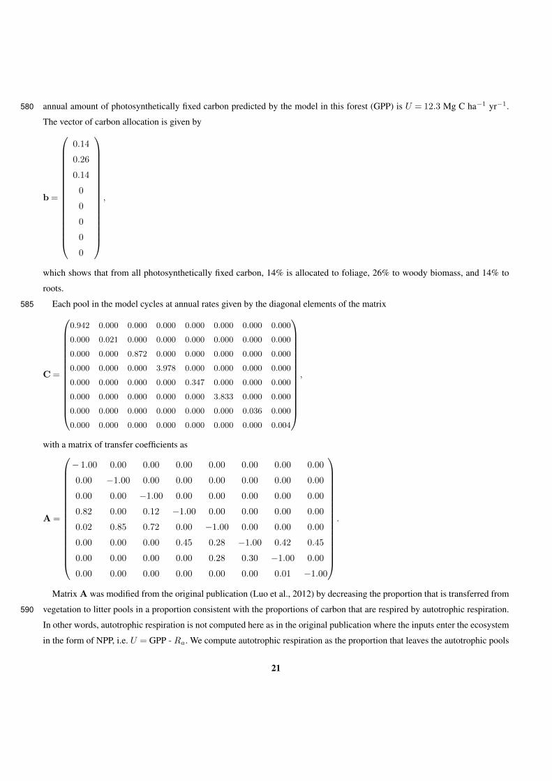
annual amount of photosynthetically fixed carbon predicted by the model in this forest (GPP) is U = 12.3 Mg C ha−1 yr−1.580

The vector of carbon allocation is given by

b =

0.14

0.26

0.14

0

0

0

0

0

,

which shows that from all photosynthetically fixed carbon, 14% is allocated to foliage, 26% to woody biomass, and 14% to

roots.

Each pool in the model cycles at annual rates given by the diagonal elements of the matrix585

C =

0.942 0.000 0.000 0.000 0.000 0.000 0.000 0.000

0.000 0.021 0.000 0.000 0.000 0.000 0.000 0.000

0.000 0.000 0.872 0.000 0.000 0.000 0.000 0.000

0.000 0.000 0.000 3.978 0.000 0.000 0.000 0.000

0.000 0.000 0.000 0.000 0.347 0.000 0.000 0.000

0.000 0.000 0.000 0.000 0.000 3.833 0.000 0.000

0.000 0.000 0.000 0.000 0.000 0.000 0.036 0.000

0.000 0.000 0.000 0.000 0.000 0.000 0.000 0.004

,

with a matrix of transfer coefficients as

A =

− 1.00 0.00 0.00 0.00 0.00 0.00 0.00 0.00

0.00 −1.00 0.00 0.00 0.00 0.00 0.00 0.00

0.00 0.00 −1.00 0.00 0.00 0.00 0.00 0.00

0.82 0.00 0.12 −1.00 0.00 0.00 0.00 0.00

0.02 0.85 0.72 0.00 −1.00 0.00 0.00 0.00

0.00 0.00 0.00 0.45 0.28 −1.00 0.42 0.45

0.00 0.00 0.00 0.00 0.28 0.30 −1.00 0.00

0.00 0.00 0.00 0.00 0.00 0.00 0.01 −1.00

.

Matrix A was modified from the original publication (Luo et al., 2012) by decreasing the proportion that is transferred from

vegetation to litter pools in a proportion consistent with the proportions of carbon that are respired by autotrophic respiration.590

In other words, autotrophic respiration is not computed here as in the original publication where the inputs enter the ecosystem

in the form of NPP, i.e. U = GPP - Ra. We compute autotrophic respiration as the proportion that leaves the autotrophic pools

21

and that is not transferred to the litter pools. In this way, U = GPP, and all carbon that is fixed enters the vegetation pools from

where it is subsequently respired or added to the litter pools.

Defining B := AC and u= bU , we obtained the steady-state solution as595

x∗ =−B−1 ·u

=

3.83

237.70

4.14

0.86

20.18

1.28

92.96

12.72

.(C1)

For the simulation with initial conditions as in a land-use-change case, the initial conditions x0 of the simulation where set

as

x0 =(

0 0 0 1.5 1.5 1.0 1.0 1.0)ᵀ◦x∗, (C2)

where the symbol ◦ represents entry-wise multiplication.600

For the transient simulations, we derived time-dependent modifiers for inputs γ(t) and for process rates ξ(t) following the

approach described in Rasmussen et al. (2016). Atmospheric CO2 concentrations increase following a sigmoid curve given by

xa(t) = 284 + 1715exp

(0.0305t

(1715 + exp(0.0305t)− 1)

), (C3)

and surface air temperature increases with CO2 concentrations according to

Ts(t) = Ts0 +σ

ln(2)ln(xa(t)/285). (C4)605

The combined effect of CO2 concentrations and air surface temperature on primary production are then computed as

γ(t) = (1 +β(xa(t),Ts(t)) ln(xa(t)/285)), (C5)

with

β(xa(t),Ts(t)) =3ρxa(t)Γ(Ts(t))

(ρxa(t)−Γ(Ts(t)))(ρxa(t) + 2Γ(Ts(t))), (C6)

where β(xa(t),Ts(t)) is the sensitivity of primary production with respect to atmospheric CO2 and air surface temperature,610

and ρ= 0.65 is the ratio of intracellular CO2 to xa(t). The response function with respect to temperature Γ(Ts(t)) is given by

Γ(Ts(t)) = 42.7 + 1.68(Ts(t)− 25) + 0.012(Ts(t)− 25)2. (C7)

22

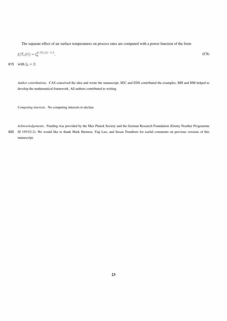
The separate effect of air surface temperatures on process rates are computed with a power function of the form

ξ(Ts(t)) = ξ0.1Ts(t)−1.5b , (C8)

with ξb = 2.615

Author contributions. CAS conceived the idea and wrote the manuscript, SEC and EDS contributed the examples, MH and HM helped to

develop the mathematical framework. All authors contributed to writing.

Competing interests. No competing interests to declare

Acknowledgements. Funding was provided by the Max Planck Society and the German Research Foundation (Emmy-Noether Programme

SI 1953/2-2). We would like to thank Mark Harmon, Yiqi Luo, and Susan Trumbore for useful comments on previous versions of this620

manuscript.

23

References

Anderson, D. H.: Compartmental modeling and tracer kinetics, Springer Science & Business Media, 1983.

Archer, D., Eby, M., Brovkin, V., Ridgwell, A., Cao, L., Mikolajewicz, U., Caldeira, K., Matsumoto, K., Munhoven, G., Montenegro, A.,

and Tokos, K.: Atmospheric Lifetime of Fossil Fuel Carbon Dioxide, Annual Review of Earth and Planetary Sciences, 37, 117–134,625

https://doi.org/10.1146/annurev.earth.031208.100206, https://doi.org/10.1146/annurev.earth.031208.100206, 2009.

Bolin, B. and Rodhe, H.: A note on the concepts of age distribution and transit time in natural reservoirs, Tellus, 25, 58–62, 1973.

Brandão, M., Levasseur, A., Kirschbaum, M. U. F., Weidema, B. P., Cowie, A. L., Jørgensen, S. V., Hauschild, M. Z., Pennington, D. W.,

and Chomkhamsri, K.: Key issues and options in accounting for carbon sequestration and temporary storage in life cycle assessment

and carbon footprinting, The International Journal of Life Cycle Assessment, 18, 230–240, https://doi.org/10.1007/s11367-012-0451-6,630

https://doi.org/10.1007/s11367-012-0451-6, 2013.

Ceballos-Núñez, V., Müller, M., and Sierra, C. A.: Towards better representations of carbon allocation in vegetation: a conceptual

framework and mathematical tool, Theoretical Ecology, in press, https://doi.org/10.1007/s12080-020-00455-w, https://doi.org/10.1007/

s12080-020-00455-w, 2020.

Chabbi, A., Lehmann, J., Ciais, P., Loescher, H. W., Cotrufo, M. F., Don, A., SanClements, M., Schipper, L., Six, J., Smith, P., and Rumpel,635

C.: Aligning agriculture and climate policy, Nature Climate Change, 7, 307 EP –, https://doi.org/10.1038/nclimate3286, 2017.

Fearnside, P. M., Lashof, D. A., and Moura-Costa, P.: Accounting for time in Mitigating Global Warming through land-use change and

forestry, Mitigation and Adaptation Strategies for Global Change, 5, 239–270, https://doi.org/10.1023/A:1009625122628, https://doi.org/

10.1023/A:1009625122628, 2000.

Grace, J.: Understanding and managing the global carbon cycle, Journal of Ecology, 92, 189–202, 2004.640

Harmon, M. E., Ferrell, W. K., and Franklin, J.: Effects on carbon storage of conversion of old-growth forests to young forests, Science, 247,

699–702, 1990.

Hespanha, J. P.: Linear Systems Theory, Princeton University Press, Princeton, New Jersey, iSBN13: 9780691179575, 2009.

IPCC: General guidance and reporting, in: 2006 IPCC guidelines for national greenhouse gas inventories, edited by Eggleston, S., Buendia,

L., Miwa, K., Ngara, T., and Tanabe, K., vol. 1, Institute for Global Environmental Strategies Hayama, Japan, 2006.645

IPCC: Climate Change 2013 – The Physical Science Basis: Working Group I Contribution to the Fifth Assessment Report of the Intergov-

ernmental Panel on Climate Change, Cambridge University Press, https://doi.org/10.1017/CBO9781107415324, 2014.

Jacquez, J. A. and Simon, C. P.: Qualitative Theory of Compartmental Systems, SIAM Review, 35, 43–79, https://doi.org/10.1137/1035003,

https://doi.org/10.1137/1035003, 1993.

Janisch, J. and Harmon, M.: Successional changes in live and dead wood carbon stores: implications for net ecosystem productivity, Tree650

Physiology, 22, 77–89, 2002.

Joos, F., Roth, R., Fuglestvedt, J. S., Peters, G. P., Enting, I. G., von Bloh, W., Brovkin, V., Burke, E. J., Eby, M., Edwards, N. R., Friedrich, T.,

Frölicher, T. L., Halloran, P. R., Holden, P. B., Jones, C., Kleinen, T., Mackenzie, F. T., Matsumoto, K., Meinshausen, M., Plattner, G.-K.,

Reisinger, A., Segschneider, J., Shaffer, G., Steinacher, M., Strassmann, K., Tanaka, K., Timmermann, A., and Weaver, A. J.: Carbon diox-

ide and climate impulse response functions for the computation of greenhouse gas metrics: a multi-model analysis, Atmospheric Chemistry655

and Physics, 13, 2793–2825, https://doi.org/10.5194/acp-13-2793-2013, https://www.atmos-chem-phys.net/13/2793/2013/, 2013.

Jung, M., Schwalm, C., Migliavacca, M., Walther, S., Camps-Valls, G., Koirala, S., Anthoni, P., Besnard, S., Bodesheim, P., Carvalhais, N.,

Chevallier, F., Gans, F., Goll, D. S., Haverd, V., Köhler, P., Ichii, K., Jain, A. K., Liu, J., Lombardozzi, D., Nabel, J. E. M. S., Nelson,

24

J. A., O’Sullivan, M., Pallandt, M., Papale, D., Peters, W., Pongratz, J., Rödenbeck, C., Sitch, S., Tramontana, G., Walker, A., Weber,

U., and Reichstein, M.: Scaling carbon fluxes from eddy covariance sites to globe: synthesis and evaluation of the FLUXCOM approach,660

Biogeosciences, 17, 1343–1365, https://doi.org/10.5194/bg-17-1343-2020, https://www.biogeosciences.net/17/1343/2020/, 2020.

Kloeden, P. E. and Rasmussen, M.: Nonautonomous dynamical systems, American Mathematical Society, 2011.

Körner, C.: A matter of tree longevity, Science, 355, 130–131, https://doi.org/10.1126/science.aal2449, https://science.sciencemag.org/

content/355/6321/130, 2017.

Lal, R.: Soil carbon sequestration impacts on global climate change and food security, Science, 304, 1623–1627, 2004.665

Lashof, D. A. and Ahuja, D. R.: Relative contributions of greenhouse gas emissions to global warming, Nature, 344, 529–531,

https://doi.org/10.1038/344529a0, https://doi.org/10.1038/344529a0, 1990.

Lu, X., Wang, Y.-P., Luo, Y., and Jiang, L.: Ecosystem carbon transit versus turnover times in response to climate warming and rising

atmospheric CO2 concentration, Biogeosciences, 15, 6559–6572, https://doi.org/10.5194/bg-15-6559-2018, https://www.biogeosciences.

net/15/6559/2018/, 2018.670

Luo, Y. and Weng, E.: Dynamic disequilibrium of the terrestrial carbon cycle under global change, Trends in Ecology & Evolution, 26,

96–104, 2011.

Luo, Y., Weng, E., and Yang, Y.: Ecosystem Ecology, in: Encyclopedia of Theoretical Ecology, edited by Hastings, A. and Gross, L., pp.

219–229, University of California Press, Berkeley, 2012.

Luo, Y., Shi, Z., Lu, X., Xia, J., Liang, J., Jiang, J., Wang, Y., Smith, M. J., Jiang, L., Ahlström, A., Chen, B., Hararuk, O., Hast-675

ings, A., Hoffman, F., Medlyn, B., Niu, S., Rasmussen, M., Todd-Brown, K., and Wang, Y.-P.: Transient dynamics of terrestrial

carbon storage: mathematical foundation and its applications, Biogeosciences, 14, 145–161, https://doi.org/10.5194/bg-14-145-2017,

https://www.biogeosciences.net/14/145/2017/, 2017.

Metzler, H. and Sierra, C. A.: Linear Autonomous Compartmental Models as Continuous-Time Markov Chains: Transit-Time and Age Dis-

tributions, Mathematical Geosciences, 50, 1–34, https://doi.org/10.1007/s11004-017-9690-1, https://doi.org/10.1007/s11004-017-9690-1,680

2018.

Metzler, H., Müller, M., and Sierra, C. A.: Transit-time and age distributions for nonlinear time-dependent compartmental systems, Proceed-

ings of the National Academy of Sciences, 115, 1150–1155, https://doi.org/10.1073/pnas.1705296115, http://www.pnas.org/content/115/

6/1150, 2018.

Millar, R. J., Nicholls, Z. R., Friedlingstein, P., and Allen, M. R.: A modified impulse-response representation of the global near-surface air685

temperature and atmospheric concentration response to carbon dioxide emissions, Atmospheric Chemistry and Physics, 17, 7213–7228,

https://doi.org/10.5194/acp-17-7213-2017, https://www.atmos-chem-phys.net/17/7213/2017/, 2017.

Minasny, B., Malone, B. P., McBratney, A. B., Angers, D. A., Arrouays, D., Chambers, A., Chaplot, V., Chen, Z.-S., Cheng, K., Das,

B. S., Field, D. J., Gimona, A., Hedley, C. B., Hong, S. Y., Mandal, B., Marchant, B. P., Martin, M., McConkey, B. G., Mul-

der, V. L., O’Rourke, S., de Forges, A. C. R., Odeh, I., Padarian, J., Paustian, K., Pan, G., Poggio, L., Savin, I., Stolbovoy, V.,690

Stockmann, U., Sulaeman, Y., Tsui, C.-C., Vågen, T.-G., van Wesemael, B., and Winowiecki, L.: Soil carbon 4 per mille, Geo-

derma, 292, 59 – 86, https://doi.org/https://doi.org/10.1016/j.geoderma.2017.01.002, http://www.sciencedirect.com/science/article/pii/

S0016706117300095, 2017.

Moura Costa, P. and Wilson, C.: An equivalence factor between CO2 avoided emissions and sequestration – description and applications in

forestry, Mitigation and Adaptation Strategies for Global Change, 5, 51–60, https://doi.org/10.1023/A:1009697625521, https://doi.org/10.695

1023/A:1009697625521, 2000.

25

Myhre, G., Shindell, D., Bréon, F.-M., Collins, W., Fuglestvedt, J., Huang, J., Koch, D., Lamarque, J.-F., Lee, D., Mendoza, B., et al.:

Anthropogenic and natural radiative forcing, in: Climate Change 2013: The Physical Science Basis. Contribution of Working Group I to

the Fifth Assessment Report of the Intergovernmental Panel on Climate Change, edited by Stocker, T., Qin, D., Plattner, G.-K., Tignor,

M., Allen, S., Boschung, J., Nauels, A., Xia, Y., Bex, V., and Midgley, P., pp. 658–740, Cambridge University Press, 2013.700

Neubauer, S. C. and Megonigal, J. P.: Moving Beyond Global Warming Potentials to Quantify the Climatic Role of Ecosystems, Ecosystems,

18, 1000–1013, https://doi.org/10.1007/s10021-015-9879-4, https://doi.org/10.1007/s10021-015-9879-4, 2015.

Noble, I., Apps, M., Houghton, R., Lashof, D., Makundi, W., Murdiyarso, D., Murray, B., Sombroek, W., , and Valentini, R.: Implications of

Different Definitions and Generic Issues, in: Land Use, Land Use Change, and Forestry, edited by Watson, R. T., Noble, I. R., Bolin, B.,

Ravindranath, N. H., Verardo, D. J., and Dokken, D. J., pp. 53–156, Cambridge University Press, 2000.705

O’Neill, B. C., Gaffin, S. R., Tubiello, F. N., and Oppenheimer, M.: Reservoir timescales for anthropogenic CO2 in the atmosphere, Tellus B,

46, 378–389, https://doi.org/10.1034/j.1600-0889.1994.t01-4-00004.x, http://dx.doi.org/10.1034/j.1600-0889.1994.t01-4-00004.x, 1994.

Prather, M. J.: Time scales in atmospheric chemistry: Theory, GWPs for CH4 and CO, and runaway growth, Geophysical Research Letters,

23, 2597–2600, https://doi.org/10.1029/96GL02371, http://dx.doi.org/10.1029/96GL02371, 1996.

Rasmussen, M., Hastings, A., Smith, M. J., Agusto, F. B., Chen-Charpentier, B. M., Hoffman, F. M., Jiang, J., Todd-Brown, K. E. O.,710

Wang, Y., Wang, Y.-P., and Luo, Y.: Transit times and mean ages for nonautonomous and autonomous compartmental systems, Journal of

Mathematical Biology, 73, 1379–1398, https://doi.org/10.1007/s00285-016-0990-8, https://doi.org/10.1007/s00285-016-0990-8, 2016.

Rodhe, H.: A Comparison of the Contribution of Various Gases to the Greenhouse Effect, Science, 248, 1217–1219,

https://doi.org/10.1126/science.248.4960.1217, http://science.sciencemag.org/content/248/4960/1217, 1990.

Rodhe, H.: Modeling biogeochemical cycles, in: Earth system science: from biogeochemical cycles to global change, edited by Jacobson,715

M. C., Charlson, R. J., Rodhe, H., and Orians, G. H., pp. 62–84, Academic Press, 2000.

Schiedung, M., Tregurtha, C. S., Beare, M. H., Thomas, S. M., and Don, A.: Deep soil flipping increases carbon stocks of New Zealand

grasslands, Global Change Biology, 25, 2296–2309, https://doi.org/10.1111/gcb.14588, https://onlinelibrary.wiley.com/doi/abs/10.1111/

gcb.14588, 2019.

Schulze, E. D., Stupak, I., and Hessenmöller, D.: The climate mitigation potential of managed versus unmanaged spruce and beech forests720

in Central Europe, in: Bioenergy with Carbon Capture and Storage, edited by Pires, J. C. M. and Gonçalves, A. L. D. C., pp. 131 –

149, Academic Press, https://doi.org/https://doi.org/10.1016/B978-0-12-816229-3.00007-7, http://www.sciencedirect.com/science/article/

pii/B9780128162293000077, 2019.

Sedjo, R. and Sohngen, B.: Carbon Sequestration in Forests and Soils, Annual Review of Resource Economics, 4, 127–144,

https://doi.org/10.1146/annurev-resource-083110-115941, https://doi.org/10.1146/annurev-resource-083110-115941, 2012.725

Shine, K., Derwent, R., Wuebbles, D., and Morcrette, J.: Radiative Forcing of Climate., in: Climate Change-The IPCC Scientific Assessment.,

edited by Houghton, J., Jenkins, G., and Ephraums, J., Cambridge Cambridge University Press, 1990.

Sierra, C., del Valle, J., and Restrepo, H.: Total carbon accumulation in a tropical forest landscape, Carbon Balance and Management, 7, 12,

https://doi.org/10.1186/1750-0680-7-12, http://www.cbmjournal.com/content/7/1/12, 2012.

Sierra, C. A.: Approaches to Model Processes at the Ecosystem Level, in: Plant Ecology, edited by Schulze, E.-D., Beck, E., Buch-730

mann, N., Clemens, S., Müller-Hohenstein, K., and Scherer-Lorenzen, M., pp. 513–527, Springer Berlin Heidelberg, Berlin, Heidelberg,

https://doi.org/10.1007/978-3-662-56233-8_15, https://doi.org/10.1007/978-3-662-56233-8_15, 2019.

Sierra, C. A., Müller, M., Metzler, H., Manzoni, S., and Trumbore, S. E.: The muddle of ages, turnover, transit, and residence times in the

carbon cycle, Global Change Biology, 23, 1763–1773, https://doi.org/10.1111/gcb.13556, http://dx.doi.org/10.1111/gcb.13556, 2017.

26

Sierra, C. A., Ceballos-Núñez, V., Metzler, H., and Müller, M.: Representing and Understanding the Carbon Cycle Using the Theory of Com-735

partmental Dynamical Systems, Journal of Advances in Modeling Earth Systems, 10, 1729–1734, https://doi.org/10.1029/2018MS001360,

2018a.

Sierra, C. A., Hoyt, A. M., He, Y., and Trumbore, S. E.: Soil Organic Matter Persistence as a Stochastic Process: Age and Transit Time

Distributions of Carbon in Soils, Global Biogeochemical Cycles, 32, 1574–1588, https://doi.org/10.1029/2018GB005950, https://agupubs.

onlinelibrary.wiley.com/doi/abs/10.1029/2018GB005950, 2018b.740

Silver, W., Ostertag, R., and Lugo, A. E.: The potential of carbon sequestration through reforestation of abandoned tropical agricultural and

pasture lands, Restoration ecology, 8, 394–407, 2000.

Weng, E. and Luo, Y.: Relative information contributions of model vs. data to short- and long-term forecasts of forest carbon dynamics,

Ecological Applications, 21, 1490–1505, https://doi.org/10.1890/09-1394.1, http://dx.doi.org/10.1890/09-1394.1, 2011.

Xia, J., Luo, Y., Wang, Y.-P., and Hararuk, O.: Traceable components of terrestrial carbon storage capacity in biogeochemical models, Global745

Change Biology, 19, 2104–2116, https://doi.org/10.1111/gcb.12172, http://dx.doi.org/10.1111/gcb.12172, 2013.

27

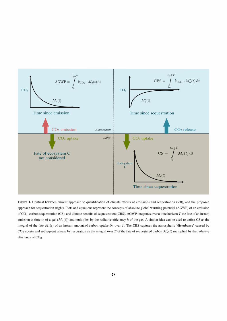
Time since emission

CO2

CO2 emission

CO2 uptake

Time since sequestration

EcosystemC

CO2 release

Time since sequestration

CO2

CO2 uptake

Fate of ecosystem Cnot considered

Land

Atmosphere

Figure 1. Contrast between current approach to quantification of climate effects of emissions and sequestration (left), and the proposed

approach for sequestration (right). Plots and equations represent the concepts of absolute global warming potential (AGWP) of an emission

of CO2, carbon sequestration (CS), and climate benefits of sequestration (CBS). AGWP integrates over a time horizon T the fate of an instant

emission at time t0 of a gas (Ma(t)) and multiplies by the radiative efficiency k of the gas. A similar idea can be used to define CS as the

integral of the fate Ms(t) of an instant amount of carbon uptake S0 over T . The CBS captures the atmospheric ‘disturbance’ caused by

CO2 uptake and subsequent release by respiration as the integral over T of the fate of sequestered carbon M ′a(t) multiplied by the radiative

efficiency of CO2.

28

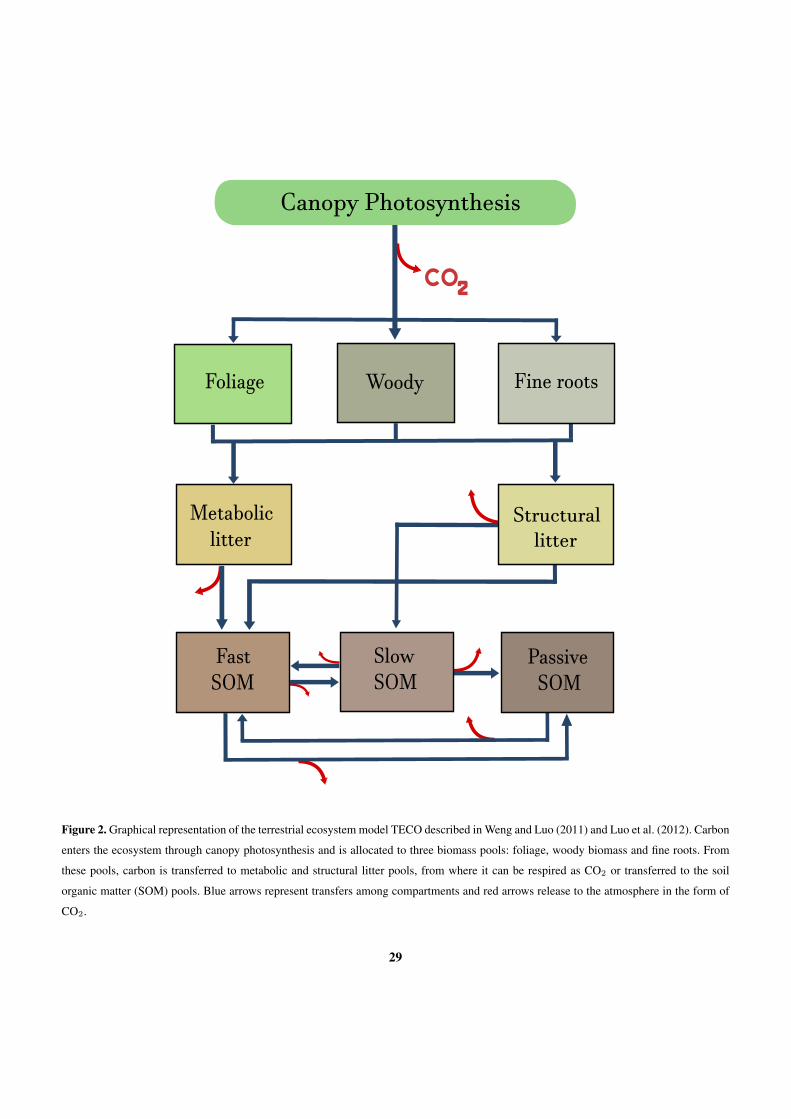
Canopy Photosynthesis

Fast SOM

Foliage Fine rootsWoody

Metabolic litter

Slow SOM

Passive SOM

Structural litter

Figure 2. Graphical representation of the terrestrial ecosystem model TECO described in Weng and Luo (2011) and Luo et al. (2012). Carbon

enters the ecosystem through canopy photosynthesis and is allocated to three biomass pools: foliage, woody biomass and fine roots. From

these pools, carbon is transferred to metabolic and structural litter pools, from where it can be respired as CO2 or transferred to the soil

organic matter (SOM) pools. Blue arrows represent transfers among compartments and red arrows release to the atmosphere in the form of

CO2.

29

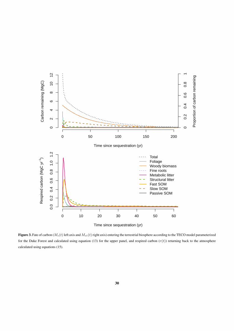
0 50 100 150 200

02

46

810

12

Time since sequestration (yr)

Car

bon

rem

aini

ng (

MgC

)

00.

20.

40.

60.

81

Pro

port

ion

of c

arbo

n re

mai

ning

0 10 20 30 40 50 60

0.0

0.2

0.4

0.6

0.8

1.0

1.2

Time since sequestration (yr)

Res

pire

d ca

rbon

(M

gC y

r−1) Total

FoliageWoody biomassFine rootsMetabolic litterStructural litterFast SOMSlow SOMPassive SOM

Figure 3. Fate of carbon (Ms(t) left axis andMs1(t) right axis) entering the terrestrial biosphere according to the TECO model parameterized

for the Duke Forest and calculated using equation (13) for the upper panel, and respired carbon (r(t)) returning back to the atmosphere

calculated using equations (15).

30

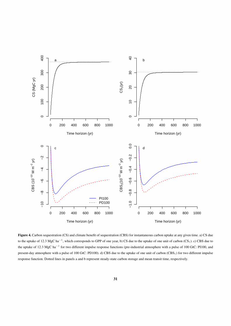
0 200 400 600 800 1000

010

020

030

040

0

Time horizon (yr)

CS

(M

gC y

r)

a

0 200 400 600 800 10000

1020

3040

Time horizon (yr)

CS

1(yr

)

b

0 200 400 600 800 1000

−10

−8

−6

−4

−2

0

Time horizon (yr)

CB

S (

10−1

0 W m

−2 y

r)

c

PI100PD100

0 200 400 600 800 1000

−1.

0−

0.8

−0.

6−

0.4

−0.

20.

0

Time horizon (yr)

CB

S1(

10−1

0 W m

−2 y

r)

d

Figure 4. Carbon sequestration (CS) and climate benefit of sequestration (CBS) for instantaneous carbon uptake at any given time. a) CS due

to the uptake of 12.3 MgC ha−1, which corresponds to GPP of one year, b) CS due to the uptake of one unit of carbon (CS1). c) CBS due to

the uptake of 12.3 MgC ha−1 for two different impulse response functions (pre-industrial atmosphere with a pulse of 100 GtC: PI100, and

present-day atmosphere with a pulse of 100 GtC: PD100). d) CBS due to the uptake of one unit of carbon (CBS1) for two different impulse

response function. Dotted lines in panels a and b represent steady-state carbon storage and mean transit time, respectively.

31

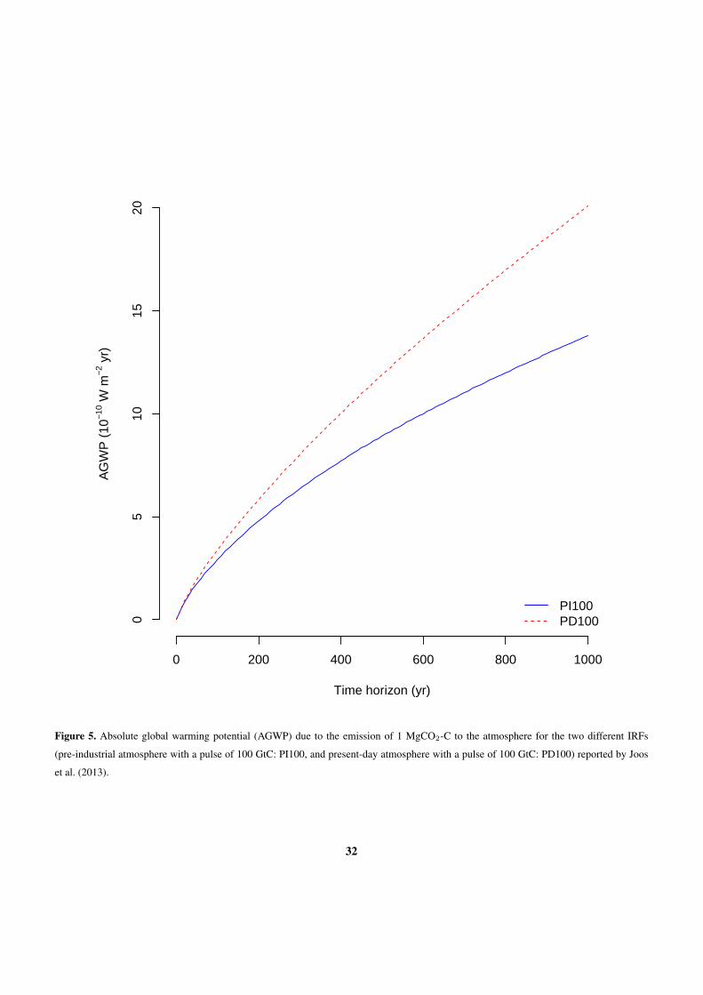
0 200 400 600 800 1000

05

1015

20

Time horizon (yr)

AG

WP

(10

−10 W

m−2

yr)

PI100PD100

Figure 5. Absolute global warming potential (AGWP) due to the emission of 1 MgCO2-C to the atmosphere for the two different IRFs

(pre-industrial atmosphere with a pulse of 100 GtC: PI100, and present-day atmosphere with a pulse of 100 GtC: PD100) reported by Joos

et al. (2013).

32

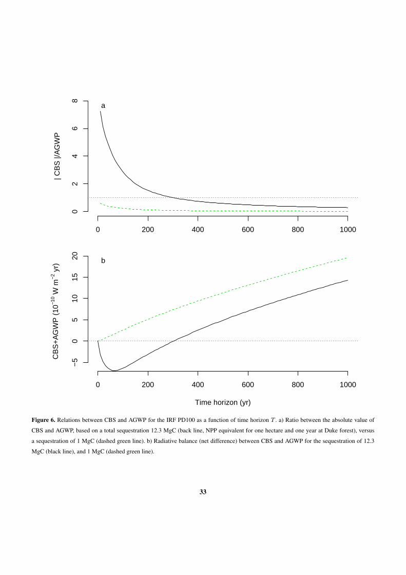
0 200 400 600 800 1000

02

46

8

| CB

S |/

AG

WP

a

0 200 400 600 800 1000

−5

05

1015

20

Time horizon (yr)

CB

S+

AG

WP

(10

−10 W

m−2

yr)

b

Figure 6. Relations between CBS and AGWP for the IRF PD100 as a function of time horizon T . a) Ratio between the absolute value of

CBS and AGWP, based on a total sequestration 12.3 MgC (back line, NPP equivalent for one hectare and one year at Duke forest), versus

a sequestration of 1 MgC (dashed green line). b) Radiative balance (net difference) between CBS and AGWP for the sequestration of 12.3

MgC (black line), and 1 MgC (dashed green line).

33

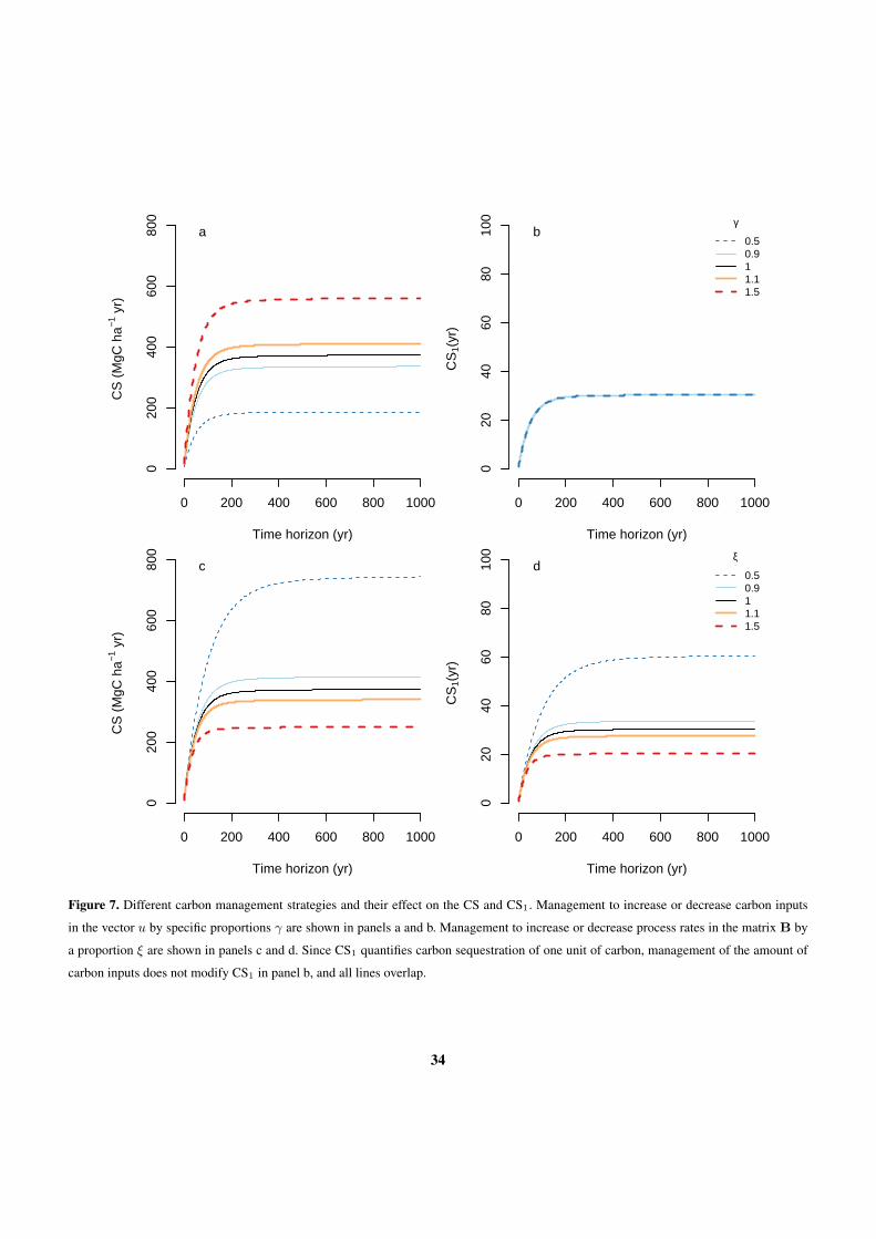
0 200 400 600 800 1000

020

040

060

080

0

Time horizon (yr)

CS

(M

gC h

a−1 y

r)

a

0 200 400 600 800 10000

2040

6080

100

Time horizon (yr)

CS

1(yr

)

bγ

0.50.911.11.5

0 200 400 600 800 1000

020

040

060

080

0

Time horizon (yr)

CS

(M

gC h

a−1 y

r)

c

0 200 400 600 800 1000

020

4060

8010

0

Time horizon (yr)

CS

1(yr

)

dξ

0.50.911.11.5

Figure 7. Different carbon management strategies and their effect on the CS and CS1. Management to increase or decrease carbon inputs

in the vector u by specific proportions γ are shown in panels a and b. Management to increase or decrease process rates in the matrix B by

a proportion ξ are shown in panels c and d. Since CS1 quantifies carbon sequestration of one unit of carbon, management of the amount of

carbon inputs does not modify CS1 in panel b, and all lines overlap.

34

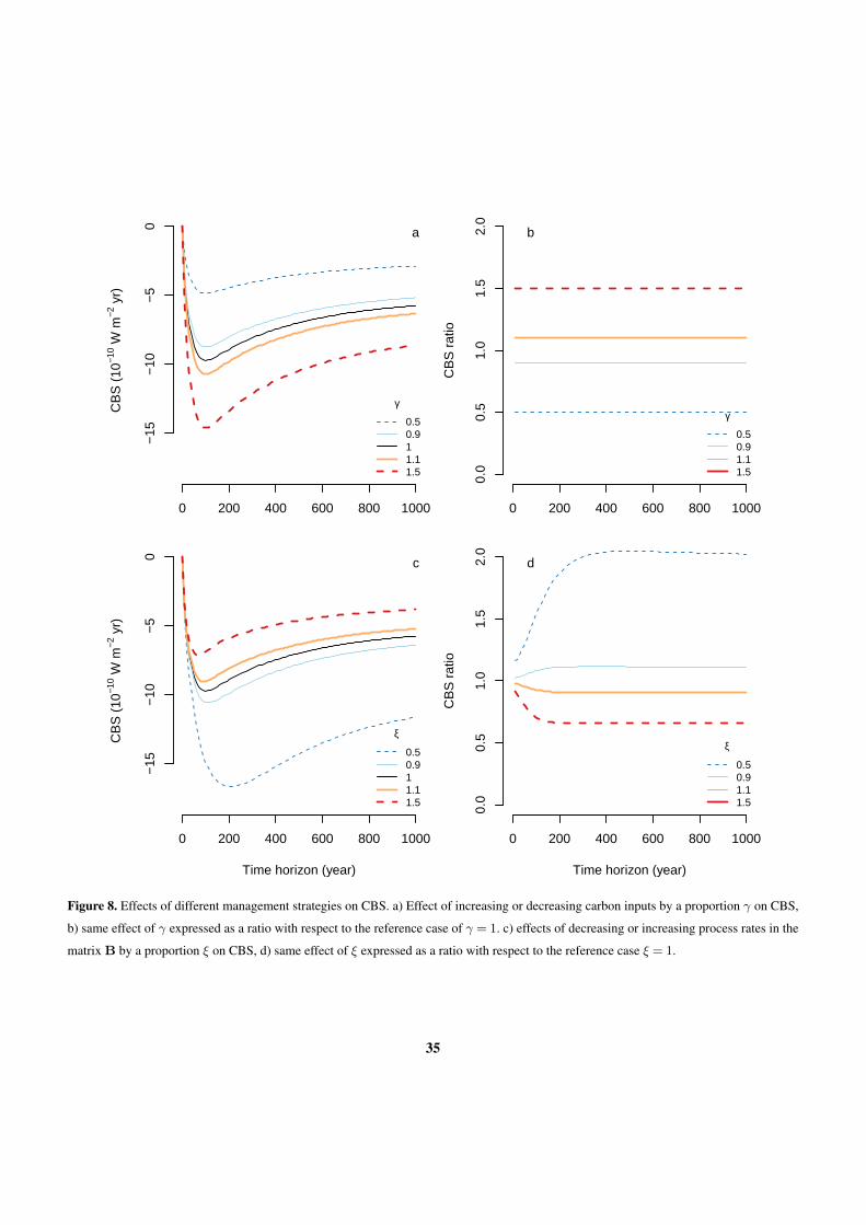
0 200 400 600 800 1000

−15

−10

−5

0

CB

S (

10−1

0 W m

−2 y

r)

γ

0.50.911.11.5

a

0 200 400 600 800 1000

0.0

0.5

1.0

1.5

2.0

CB

S r

atio

γ

0.50.91.11.5

b

0 200 400 600 800 1000

−15

−10

−5

0

Time horizon (year)

CB

S (

10−1

0 W m

−2 y

r)

ξ

0.50.911.11.5

c

0 200 400 600 800 1000

0.0

0.5

1.0

1.5

2.0

Time horizon (year)

CB

S r

atio

ξ

0.50.91.11.5

d

Figure 8. Effects of different management strategies on CBS. a) Effect of increasing or decreasing carbon inputs by a proportion γ on CBS,

b) same effect of γ expressed as a ratio with respect to the reference case of γ = 1. c) effects of decreasing or increasing process rates in the

matrix B by a proportion ξ on CBS, d) same effect of ξ expressed as a ratio with respect to the reference case ξ = 1.

35

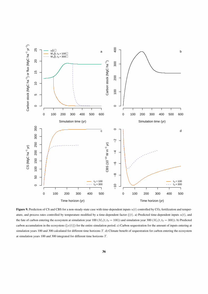
0 100 200 300 400 500 600

05

1015

2025

Simulation time (yr)

Car

bon

stoc

k (M

gC h

a−1)

or fl

ux (

MgC

ha−1

yr−1

)

u(t)Ms(t, t0 = 100)Ms(t, t0 = 300)

a

0 100 200 300 400 500 6000

100

200

300

400

Simulation time (yr)

Car

bon

stoc

k (M

gC h

a−1)

b

0 100 200 300 400 500

050

100

150

200

250

300

350

Time horizon (yr)

CS

(M

gC h

a−1 y

r)

t0 = 100t0 = 300

c

0 100 200 300 400 500

−10

−8

−6

−4

−2

0

Time horizon (yr)

CB

S (

10−1

0 W m

−2 y

r)

t0 = 100t0 = 300

d

Figure 9. Prediction of CS and CBS for a non-steady-state case with time-dependent inputs u(t) controlled by CO2 fertilization and temper-

ature, and process rates controlled by temperature modified by a time-dependent factor ξ(t). a) Predicted time-dependent inputs u(t), and

the fate of carbon entering the ecosystem at simulation year 100 (Ms(t, t0 = 100)) and simulation year 300 (Ms(t, t0 = 300)). b) Predicted

carbon accumulation in the ecosystem (‖x(t)‖) for the entire simulation period. c) Carbon sequestration for the amount of inputs entering at

simulation years 100 and 300 calculated for different time horizons T . d) Climate benefit of sequestration for carbon entering the ecosystem

at simulation years 100 and 300 integrated for different time horizons T .

36

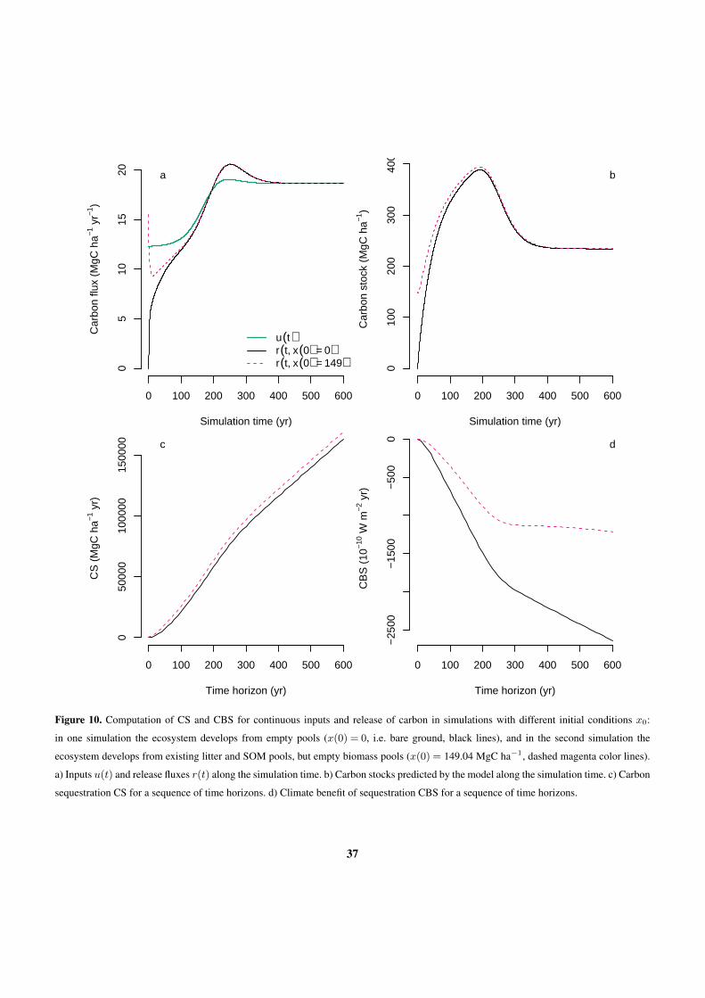
0 100 200 300 400 500 600

05

1015

20

Simulation time (yr)

Car

bon

flux

(MgC

ha−1

yr−1

)

u(t)r(t, x(0) = 0)r(t, x(0) = 149)

a

0 100 200 300 400 500 6000

100

200

300

400

Simulation time (yr)

Car

bon

stoc

k (M

gC h

a−1)

b

0 100 200 300 400 500 600

050

000

1000

0015

0000

Time horizon (yr)

CS

(M

gC h

a−1 y

r)

c

0 100 200 300 400 500 600

−25

00−

1500

−50

00

Time horizon (yr)

CB

S (

10−1

0 W m

−2 y

r)

d

Figure 10. Computation of CS and CBS for continuous inputs and release of carbon in simulations with different initial conditions x0:

in one simulation the ecosystem develops from empty pools (x(0) = 0, i.e. bare ground, black lines), and in the second simulation the

ecosystem develops from existing litter and SOM pools, but empty biomass pools (x(0) = 149.04 MgC ha−1, dashed magenta color lines).

a) Inputs u(t) and release fluxes r(t) along the simulation time. b) Carbon stocks predicted by the model along the simulation time. c) Carbon

sequestration CS for a sequence of time horizons. d) Climate benefit of sequestration CBS for a sequence of time horizons.

37