Draft version June 15, 2018Preprint typeset using LATEX style emulateapj v. 11/10/09

GALAXIES IN X-RAY GROUPS I: ROBUST MEMBERSHIP ASSIGNMENT AND THE IMPACT OF GROUPENVIRONMENTS ON QUENCHING

Matthew R. George1,2, Alexie Leauthaud2,3, Kevin Bundy1, Alexis Finoguenov4,5, Jeremy Tinker6,Yen-Ting Lin7,8, Simona Mei9,10, Jean-Paul Kneib11, Herve Aussel12, Peter S. Behroozi13, Michael T. Busha13,14,

Peter Capak15, Lodovico Coccato16, Giovanni Covone17, Cecile Faure18, Stephanie L. Fiorenza19,Olivier Ilbert11, Emeric Le Floc’h12, Anton M. Koekemoer20, Masayuki Tanaka7, Risa H. Wechsler13,

Melody Wolk21

Draft version June 15, 2018

ABSTRACT

Understanding the mechanisms that lead dense environments to host galaxies with redder col-ors, more spheroidal morphologies, and lower star formation rates than field populations remains animportant problem. As most candidate processes ultimately depend on host halo mass, accurate char-acterizations of the local environment, ideally tied to halo mass estimates and spanning a range inhalo mass and redshift are needed. In this work, we present and test a rigorous, probabalistic methodfor assigning galaxies to groups based on precise photometric redshifts and X-ray selected groupsdrawn from the COSMOS field. The groups have masses in the range 1013 . M200c/M . 1014

and span redshifts 0 < z < 1. We characterize our selection algorithm via tests on spectroscopicsubsamples, including new data obtained at the VLT, and by applying our method to detailed mockcatalogs. We find that our group member galaxy sample has a purity of 84% and completeness of92% within 0.5R200c. We measure the impact of uncertainties in redshifts and group centering on thequality of the member selection with simulations based on current data as well as future imaging andspectroscopic surveys. As a first application of our new group member catalog which will be madepublicly available, we show that member galaxies exhibit a higher quenched fraction compared to thefield at fixed stellar mass out to z ∼ 1, indicating a significant relationship between star formationand environment at group scales. We also address the suggestion that dusty star forming galaxiesin such groups may impact the high-` power spectrum of the cosmic microwave background and findthat such a population cannot explain the low power seen in recent SZ measurements.

Subject headings: catalogs – galaxies: groups: general – galaxies: star formation

mgeorge@astro.berkeley.edu1 Department of Astronomy, University of California, Berke-

ley, CA 94720, USA2 Lawrence Berkeley National Laboratory, 1 Cyclotron Road,

Berkeley CA 94720, USA3 Berkeley Center for Cosmological Physics, University of Cal-

ifornia, Berkeley, CA 94720, USA4 Max-Planck-Institut fur Extraterrestrische Physik, Giessen-

bachstraße, 85748 Garching, Germany5 University of Maryland Baltimore County, 1000 Hilltop Cir-

cle, Baltimore, MD 21250, USA6 Center for Cosmology and Particle Physics, Department of

Physics, New York University, 4 Washington Place, New York,NY 10003, USA

7 Institute for the Physics and Mathematics of the Universe,The University of Tokyo, Kashiwa, Chiba 277-8568, Japan

8 Institute of Astronomy & Astrophysics, Academia Sinica,Taipei, Taiwan

9 University of Paris Denis Diderot, 75205 Paris CEDEX 13,France

10 GEPI, Observatoire de Paris, Section de Meudon, 92195Meudon CEDEX, France

11 Laboratoire d’Astrophysique de Marseille, CNRS Univer-site de Provence, 38 rue F. Joliot-Curie, 13388 Marseille Cedex13, France

12 Service d’Astrophysique, CEA-Saclay, Orme de Merisiers,Bat. 709, 91191 Gif-sur-Yvette, France

13 Kavli Institute for Particle Astrophysics and Cosmology;Physics Department, Stanford University; and SLAC NationalAccelerator Laboratory, Stanford CA 94305, USA

14 Institute for Theoretical Physics, University of Zurich, 8057Zurich, Switzerland

15 Spitzer Science Center, 314-6 Caltech, 1201 East CaliforniaBoulevard, Pasadena, CA, 91125, USA

16 European Southern Observatory, Karl-Schwarzchild-str. 2,

85748 Garching, Germany17 Universita di Napolia Federico II, Dipartimento di Sciennze

Fisiche and INAF Observatorio Astronomico di Capodimonte,v. Moiariello 16, 80131 Napoli, Italy

18 Laboratoire d’Astrophysique, Ecole Polytechnique Federalede Lausanne (EPFL), Observatoire de Sauverny, 1290 Versoix,Switzerland

19 Astrophysical Observatory, City University of New York,College of Staten Island, 2800 Victory Blvd., Staten Island, NY10314, USA

20 Space Telescope Science Institute, 3700 San Martin Drive,Baltimore, MD 21218, USA

21 Institut d’Astrophysique de Paris, UMR 7095, 98 bis Boule-vard Arago, 75014 Paris, France

arX

iv:1

109.

6040

v1 [

astr

o-ph

.CO

] 2

7 Se

p 20

11

2 George et al.

1. INTRODUCTION

Galaxies in dense cluster regions have long been knownto have different characteristics than counterparts inthe field, with redder colors, a greater tendency forspheroidal morphologies, and suppressed star formationrates. Dense clusters are also the sites of the most mas-sive and luminous galaxies. Much effort has been made tofind the redshift, halo mass, and cluster-centric distanceat which these distinctions between galaxy populationsare imprinted and the process by which these transforma-tions occur (e.g., Oemler 1974; Dressler 1980; Butcher &Oemler 1984; Dressler et al. 1997; Poggianti et al. 1999;Lewis et al. 2002; Goto et al. 2003; Balogh et al. 2004; DePropris et al. 2004; Kauffmann et al. 2004; Lin et al. 2004;Blanton et al. 2005; Cucciati et al. 2006; Cooper et al.2006; Weinmann et al. 2006; Capak et al. 2007a; Gerkeet al. 2007; Blanton & Moustakas 2009; Hansen et al.2009; Mei et al. 2009; Feruglio et al. 2010). While mas-sive clusters present clear examples of galaxy transfor-mations due to gas stripping, merger activity, and tidaldisruption (e.g., Kenney et al. 1995; Gavazzi et al. 2001;Cortese et al. 2007), the extent to which these processesaffect the majority of galaxies which live in less denseenvironments is uncertain. Extending cluster samples togroups with lower halo masses and higher redshifts ischallenging because it requires significant observationalexpenditures and careful analysis to isolate such environ-ments from the field.

Recent analyses at low redshift have confirmed the ex-istence of an environmental dependence of galactic struc-ture and colors across a range of environments (e.g.,Kauffmann et al. 2004; Baldry et al. 2006; Bamfordet al. 2009). The corresponding picture at z ∼ 1 hasbeen less clear. With pointed observations around high-redshift galaxy clusters, several studies have found sig-nificant trends in morphology, color, and star-formationrate with local galaxy density (e.g., Postman et al. 2005;Smith et al. 2005; Tanaka et al. 2005; Poggianti et al.2008). However, some find that the relations disappearin stellar mass-selected samples, arguing that environ-mental trends are due to differences in the stellar massdistribution between environments rather than physicalprocesses acting in dense regions (e.g., Poggianti et al.2008).

In field surveys reaching z ∼ 1, results from theVIRMOS-VLT Deep Survey (VVDS; Scodeggio et al.2009) and zCOSMOS (Tasca et al. 2009; Cucciati et al.2010; Iovino et al. 2010; Kovac et al. 2010a) show littleor no environmental influence on morphology and colorespecially at high stellar masses (log(M?/M) & 10.7),while results from DEEP2 (Cooper et al. 2010) and oth-ers from zCOSMOS (Peng et al. 2010) show a clear rela-tionship between color and environment. These papersgenerally find weakening environmental trends with in-creasing redshift, but differ in the redshift at which thetrends disappear. Cooper et al. (2007) and Cooper et al.(2010) discuss the discrepancies in environmental trendsseen in high-redshift field surveys and suggest that thenon-detection by some studies could be due to the useof less confident spectroscopic redshifts and lower sam-pling rates, as well as increased difficulty with determin-ing environmental densities using optical spectroscopyat high redshift, while Peng et al. (2010) attributes the

differences to the definitions used to characterize envi-ronments.

The aim of this work is to define a clean sample ofgalaxies in dense group environments out to redshiftz = 1 to address these issues. We study groups fromthe COSMOS survey that have been identified as sourcesof extended X-ray emission (Finoguenov et al. 2007,and in prep.), which is a strong indication that theyare virialized structures and not chance associations ofgalaxies. The groups have halo masses in the range1013 . M200c/M . 1014 as determined by weak lens-ing (Leauthaud et al. 2010). In a companion paper, wedescribe weak lensing tests to optimize the identificationof halo centers (Paper II; George et al., in prep.). Weselect member galaxies based on photometric redshiftsderived from extensive multi-wavelength imaging, whichprovides a much greater sampling density than existingspectroscopic surveys. Using a spectroscopic subsampleand mock catalogs, we carefully evaluate our memberselection for potential biases or contamination, and ac-count for photometric redshift uncertainties. This robustsample of group members can be used to address unset-tled questions about the link between galaxies and theirenvironments.

A key challenge is to disentangle the intrinsic and ex-trinsic factors that may play a role in shaping galaxyproperties. For instance, galaxies in dense regions have ahigher characteristic stellar mass than in less dense envi-ronments (e.g., Baldry et al. 2006), so a morphology-massrelation could be conflated with a morphology-density re-lation. Since stellar mass plays an important role in de-termining galaxy properties, and mass-to-light ratios arestrongly affected by star formation activity, recent envi-ronmental studies have stressed the use of stellar mass-selected samples rather than luminosity-selected samplesto make a fair comparison across environments (e.g., vander Wel et al. 2007; Scodeggio et al. 2009; Cooper et al.2010).

In addition to controlling for intrinsic galaxy proper-ties in these studies, defining and measuring the “en-vironment” presents another problem. The distance tothe Nth nearest neighbor or the mean density of galax-ies inside a fixed radius are commonly used as environ-mental indicators (e.g., Dressler 1980). Kauffmann et al.(2004) show that galaxy properties correlate most tightlywith local density on scales below ∼ 1 Mpc and areuncorrelated with the density on larger scales once thesmall-scale density is fixed. Several studies have shownevidence that galaxy properties correlate most tightlywith density within their halo, and have emphasized thatthe aperture used for comparing equivalent regions mustscale with halo mass to avoid confusion between localand global densities (Hansen et al. 2005; Weinmann et al.2006; Blanton & Berlind 2007; Haas et al. 2011). Insteadof using the galaxy density field to define environment,one can define a catalog of galaxy groups and clustersand study their properties as a function of halo massand group-centric distance. In this paper we use theterm “group” to denote a set of galaxies with a commondark matter halo and to emphasize the low mass rangestudied, making no formal distinction between groupsand clusters.

Catalogs of galaxy groups have been constructed fromboth optical surveys identifying galaxy overdensities and

Galaxies in X-ray Groups 3

X-ray surveys detecting the hot gas trapped by deepgravitational potentials. Optical catalogs often employmatched filters (e.g., Postman et al. 1996) and tesse-lations (e.g., Marinoni et al. 2002; Gerke et al. 2005)to isolate groups from the background field, and redsequence methods have proven efficient at identifyinggroups over large volumes (e.g., Gladders & Yee 2005;Koester et al. 2007). These catalogs typically assign thebrightest member galaxy as the center of each group, anduse the richness determined by the number of membersas a proxy for the total mass. X-ray detections can re-duce the likelihood of projection effects, improve massestimates, help with the determination of group centers,and shed light on the interplay between the hot gas andstellar content of groups (e.g., Mulchaey et al. 2003; Linet al. 2004; Finoguenov et al. 2007; Sun et al. 2009).

Our understanding of group properties has benefitedfrom small, well-studied samples at low redshift (e.g.,Mulchaey & Zabludoff 1998; Zabludoff & Mulchaey 1998;Tran et al. 2001; Sun et al. 2009) along with larger sta-tistical samples taken over wide areas or to high redshifts(e.g., Eke et al. 2004; Gerke et al. 2005; Gladders & Yee2005; Miller et al. 2005; Yang et al. 2005; Berlind et al.2006; Hansen et al. 2009). These studies have establishedmany similarities between groups and more massive clus-ters, including their extended dark matter halos and el-evated fractions of quenched early type galaxies relativeto the field. Groups show some differences from clustersincluding gas mass fractions that are typically lower inless massive systems, and the differences between phys-ical processes acting on galaxies in groups and those inclusters are still being explored. Recent and ongoing sur-veys are pushing to greater sample sizes and higher red-shifts with multi-wavelength observations and spectro-scopic campaigns (e.g., Osmond & Ponman 2004; Driveret al. 2009; Milkeraitis et al. 2010; Adami et al. 2010).Several large imaging surveys in development plan tostudy the growth of structure without significant spectro-scopic observations initially (Dark Energy Survey1, Hy-per Suprime-Cam2, Large Synoptic Survey Telescope3,EUCLID4), so photometric redshifts will be importantfor identifying member galaxies using techniques such asthose outlined in this paper.

We study groups in the COSMOS field where a uniquedata set has been compiled for studying the interplaybetween galaxies, intragroup gas, and dark matter ingalaxy groups out to z ∼ 1. The COSMOS survey hasobtained X-ray observations for group detections, deepimaging data spanning ultraviolet (UV), optical, and in-frared (IR) wavelengths for precise photometric redshiftsand stellar masses, extensive spectroscopic coverage, andhigh resolution imaging from the Hubble Space Tele-scope (HST) for measuring morphologies and weak lens-ing. Group catalogs have been constructed in this fieldfrom X-ray data (Finoguenov et al. 2007, and in prep.),zCOSMOS spectroscopy (Knobel et al. 2009), photomet-ric redshifts (Gillis & Hudson 2011), CFHTLS-Deep pho-tometry (Olsen et al. 2007; Grove et al. 2009), and witha combination of weak lensing and matched filters (Bel-

1 http://www.darkenergysurvey.org2 http://sumire.ipmu.jp/en3 http://www.lsst.org4 http://sci.esa.int/euclid

lagamba et al. 2011). Additionally, Scoville et al. (2007)studied large-scale structures in this field using photo-metric redshifts, and Kovac et al. (2010b) measured thegalaxy density field using zCOSMOS redshifts to probea large dynamic range of environments. Here we focuson the X-ray selected group catalog to ensure a puresample of virialized structures whose masses have beencharacterized with weak lensing (Leauthaud et al. 2010).Giodini et al. (2009) have studied the stellar mass con-tent of these X-ray groups; we expand upon their workwith a thorough characterization of a new member selec-tion algorithm and develop a group member catalog fora variety of applications.

The data used in making our group catalog are de-scribed in § 2. In § 3, we present the sample selectionand sensitivity limits, along with tests of the quality ofthe photometric redshifts constructed from the imagingdata. Our selection algorithm for the member catalogis described in § 4, where we associate member galaxieswith groups based on their proximity to the X-ray centerand their photometric redshifts. In § 5, we characterizethe reliability of our selection with mock catalogs fromsimulations and by comparing our photometric redshiftselection to the subsample of sources with spectroscopicredshifts. We make the catalog of group membership as-signments and galaxy properties publicly available, de-scribing the format and release in § 6. We discuss in § 7some of our initial findings from the catalog, includingthe influence of the group environment on galaxy col-ors out to z ∼ 1. We find evidence of suppressed starformation in galaxies in group environments over the en-tire redshift range studied, and briefly discuss how thelow incidence of star forming galaxies in groups cannotplay a significant role in explaining recent observationsof a deficit of power from the Sunyaev-Zel’dovich effect(SZ; Sunyaev & Zeldovich 1972) in the angular spectrumof the cosmic microwave background (CMB; e.g., Luekeret al. 2010; Fowler et al. 2010).

We adopt a WMAP5 ΛCDM cosmology to determinedistances and halo masses with Ωm = 0.258, ΩΛ = 0.742,H0 = 72 km s−1 Mpc−1 (Dunkley et al. 2009), the samevalues used by Leauthaud et al. (2010) to calibrate themasses of this group sample. Distances are expressedin physical units of Mpc, magnitudes are given on theAB system, X-ray luminosities are expressed in the rest-frame 0.1-2.4 keV band, and logarithmic quantities usebase 10. Group masses are estimated from their X-ray lu-minosity using the LX−M relation derived in Leauthaudet al. (2010) and concentrations are then derived fromthe mass-concentration relation of Zhao et al. (2009)assuming an NFW density profile (Navarro, Frenk, &White 1996). We estimate the virial radius of groupsas R200c, the radius within which the mean density is200 times the critical density of the Universe at the red-shift of the group, ρc(zG), and use the corresponding halomasses defined as M200c ≡ (200ρc(zG))(4π/3)R200c

3.We also make use of the NFW scale radius, defined asRs = R200c/c200c, where c200c is the concentration pa-rameter.

2. COSMOS DATA

The COSMOS field has been observed in a broad rangeof wavelengths, with imaging data from X-ray to ra-dio and a large spectroscopic follow-up program (zCOS-

4 George et al.

MOS) with the Very Large Telescope (VLT) (Scovilleet al. 2007; Koekemoer et al. 2007; Lilly et al. 2007).We have added to the spectroscopic sample in groupswith a recent campaign using the Focal Reducer and lowdispersion Spectrograph 2 (FORS2) at the VLT (Pro-gram ID 084.B-0523; PI: Mei). X-ray imaging has beentaken with the XMM-Newton (1.5 Ms covering 2.13 deg2;Hasinger et al. 2007; Cappelluti et al. 2009) and Chan-dra observatories (1.8 Ms covering 0.9 deg2; Elvis et al.2009). Imaging obtained through the F814W filter of theWide Field Channel (WFC) of the Advanced Camera forSurveys (ACS) on HST adds accurate shape measure-ments for morphologies and weak lensing (Scarlata et al.2007; Leauthaud et al. 2007). Observations of over thirtyphotometric bands covering the ultraviolet, optical, andinfrared ranges have enabled the determination of pre-cise photometric redshifts (Capak et al. 2007b; Ilbertet al. 2009), with typical redshift uncertainty σP . 0.01for galaxies with F814W < 22.5, and σP = 0.03 forF814W=24, at z < 1.2 (see §§ 2.3 and 3.2 for details andtests of the photometric redshifts used in this paper).

2.1. X-ray Catalog

The entire COSMOS region has been mapped through54 overlapping XMM-Newton pointings and additionalChandra observations covering the central region (0.9deg2) with higher spatial resolution. A mosaic combiningthese two data sets has been used to find and measurethe fluxes of groups using a wavelet transform methoddescribed in Vikhlinin et al. (1998). The data reduc-tion process including the combination of X-ray data setsand identification of optical counterparts follows that ofFinoguenov et al. (2009); Finoguenov et al. (2010). Aninitial group catalog from the COSMOS field is presentedin Finoguenov et al. (2007).

Briefly, extended objects are detected in the mosaicwhen the sum of the flux on scales of 32′′ and 64′′ isgreater than the flux on small scales by a given threshold.Detections on smaller scales tend to be contaminated bypoint sources, which are cleaned from XMM and Chan-dra data separately to allow for variability. The flux iscalculated using a scaling relation that incorporates a β-model fit to the surface brightness within 32′′, resultingin a 4σ detection limit of the group sample of 1.0×10−15

erg cm−2 s−1 over 96% of the ACS field. Once extendedX-ray sources are detected, a red sequence finder is em-ployed on galaxies with a projected distance less than0.5 Mpc from the centers to identify an optical counter-part and determine the redshift of the group, which isthen refined with spectroscopic redshifts when available.The red sequence finder only requires an overdensity ofred galaxies and not a deficiency of blue galaxies, mean-ing that it does not specifically require an enhanced redfraction to identify groups.

A quality flag (hereafter xflag) is assigned to the re-liability of the optical counterpart, with flags 1 and 2 in-dicating a secure association, and higher flags indicatingpotential problems due to projections with other sourcesor bad photometry due to bright stars in the foreground.We run our membership algorithm on all detections inthe catalog with zG < 1 but in later analyses limit thesample to groups with xflag = 1 and 2, which have re-liable spectroscopically confirmed optical counterparts.

The difference in these two flags reflects the uncertaintyin the X-ray position; for xflag = 2 the uncertainty ineach coordinate is assumed equal to the wavelet scale of32′′, and for xflag = 1 sources, which have more certaincenters, the uncertainty is 32′′ divided by the significanceof the flux measurement. The mean uncertainty in rightascension and declination for sources with flags 1 and 2is 23′′ (120 kpc at z = 0.4 and 170 kpc at z = 0.8 for ouradopted cosmology).

The main changes from the catalog described inFinoguenov et al. (2007) are the detection of faintergroups thanks to deeper XMM coverage, a more con-servative point-source removal procedure, increased red-shift accuracy due to the availability of more spectro-scopic data and improved photometric redshifts, andsome changes in quality flags after visual inspection ofoptical counterparts. In total, the catalog used in thispaper contains 211 extended X-ray sources over 1.64deg2, spanning the redshift range 0 < z < 1 and witha rest-frame 0.1–2.4 keV luminosity range of 41.3 <log(LX/erg s−1) < 44.1, and 165 of these groups andclusters have secure optical counterparts with xflag = 1or 2. X-ray detections without clear optical counter-parts are likely a mix of unresolved active galactic nuclei(AGN), projections of multiple systems, and backgroundfluctuations; tests of the identification method using alarger spectroscopic sample will be presented with theupdated X-ray catalog in a separate paper (Finoguenovet al., in prep.).

2.2. Spectroscopic Data

The COSMOS field has been targeted by a numberof spectroscopic campaigns. We use spectra from thezCOSMOS “20K sample” (Lilly et al., in prep.) whichtargeted galaxies in the ACS area to a magnitude limit ofi+ = 22.5, along with other spectroscopic data sets fromKeck, MMT, SDSS, and VLT (Prescott et al. 2006; Ca-pak et al. 2010). We include in this paper a new samplefrom our recent program with FORS2/VLT (see § 2.2.1).Each redshift has an associated confidence flag; we useonly those of class 3 or 4 meaning that the redshift is se-cure or very secure. In repeat observations, zCOSMOStargets with these confidence classes have a verificationrate of > 99% (Lilly et al. 2007). For galaxies in theACS field with F814W < 24.2 and any redshift passingthis quality cut, the spectroscopic sample has 529 galax-ies from FORS2, 11619 from zCOSMOS, and 1527 fromother sources. These spectra are distributed through-out the redshift range used in this paper, with 1931 at0.05 < z ≤ 0.25, 4257 at 0.25 < z ≤ 0.50, 4184 at0.50 < z ≤ 0.75, and 1980 at 0.75 < z ≤ 1.00.

A spectroscopically-selected group catalog has beenconstructed by Knobel et al. (2009). We defer adetailed comparison between the galaxy content ofspectroscopically-selected groups and X-ray selectedgroups to future work (Finoguenov et al., in prep.).Kovac et al. (2010b) showed that there is good gen-eral correspondence between the overdense regions inthe galaxy density field, the spectroscopically-selectedgroups with Nmem ≥ 4, and the X-ray detected groups.

Our primary use of the spectra is to obtain precisegroup redshifts and to verify the accuracy of photomet-ric redshifts, which are critical for both the membershipselection and the weak lensing analysis. Roughly 20% of

Galaxies in X-ray Groups 5

group members have spectroscopic redshifts in additionto the photometric redshifts used for member selection.

2.2.1. FORS2 Spectra

We have recently obtained additional spectra of galax-ies in the COSMOS field with the FORS2 spectrographat the VLT. Targets were selected for a number of scien-tific goals including velocity dispersion measurements ofmassive central galaxies and a comparison sample of fieldellipticals, a study of merger rates within groups based onthe abundance of close pairs, and refined redshift deter-minations for group members. Data were taken on fourclear nights with excellent conditions and 0.8′′ typicalseeing from 2010 February 14-18. The FORS2 instru-ment was used in MXU mode with the 600RI grism andGG435 order separation filter, providing a wavelengthrange of roughly 4500 − 9000A. There were 27 maskseach observed in 4 exposures of 650 seconds. Each maskhad roughly 50 slits of width 0.6′′ for bright targets and1′′ for fainter ones, and a typical slit length of 8′′.

These data have been reduced using the standard es-orex reduction pipeline5. In short, for each mask anddetector we performed bias subtraction and overscan re-moval, determined a wavelength solution from He, HgCd,Ar, and Ne arc lamps, and found slit extraction regionsusing a pattern recognition algorithm on the arc and flatlamp exposures. Science exposures were bias subtractedand flat fielded before a median combination. The flatfields were first normalized by dividing out a smoothcomponent calculated using a 10× 10 pixel median filterto account for the intrinsic shape of the flat lamp spec-trum. A local sky subtraction was performed on eachCCD column prior to rectification, then cosmic rays wereremoved and object spectra were optimally extracted.

For the extracted objects, we measured redshifts witha modified version of the zspec software used for theDEEP2 survey (Cooper et al., in prep.). Each one-dimensional spectrum was fit by a linear combinationof galaxy eigenspectra and also compared with stellarand quasar templates over a range of redshifts to findpossible redshift values. Spectral features important forfitting in this range of wavelengths and redshifts include[O II], CaK, CaH, G-Band, Hβ, [O III], Mgb, and NaD.Each spectrum was visually inspected by at least twoco-authors alongside the two-dimensional spectral imageto choose the best redshift and assign a quality flag ac-cording to the zCOSMOS system (Lilly et al. 2007). Incases where the first two inspectors disagreed on the red-shift or quality flag, a third person viewed the spectrumindependently to reconcile differences. We include onlythose objects with a secure redshift (quality flag = 3,4) inour sample, which amounts to 529 galaxies. Our redshiftsuccess rate will improve with continuing reduction ef-forts to handle cases where slits were tilted to cover closepairs or to measure velocity dispersions along the majoraxis of a galaxy. There are 8 objects in this sample thathave been observed by SDSS, with a median and scatterbetween redshift measurements of 16 and 43km s−1, re-spectively. For 126 objects observed by both FORS2 andzCOSMOS, the scatter in redshifts is 160 km s−1 afterremoving 2 outliers with |∆z| > 0.002. We have detected

5 http://www.eso.org/cpl/esorex.html

a median offset of ∼ 100 km s−1 between zCOSMOS red-shifts and those measured by FORS2 and SDSS which isstill under investigation, but since the magnitude of thisoffset is a factor of 3 smaller than the typical group veloc-ity dispersion and several times smaller than photometricredshift errors it should not impact our results.

2.3. Photometric Redshifts

Despite the extensive spectroscopic data available, cov-erage of group members is incomplete. We instead usephotometric redshifts (hereafter photo-zs) to determinedistances to galaxies. Ilbert et al. (2009) constructedspectral energy distributions (SEDs) from over 30 bandsof UV, optical, and IR data described in Capak et al.(2007b), and compared these SEDs with templates fromgalaxies at known redshifts supplemented with stellarpopulation synthesis models. They computed photo-zsfrom SEDs using a χ2 template fitting method whichincluded a treatment of emission lines. The derivedχ2(z) function was used to compute a probability den-sity function (PDF), P(z), which is the likelihood thata galaxy lives at a redshift z given the photometric dataand the spectral templates used. Rather than collaps-ing this function to a single value at the mean, median,or peak and assuming Gaussian uncertainty as is oftendone, we make use of the full PDF to determine groupmembership, described in § 4. In this paper we use an up-dated version (pdzBay v1.7 010809) of the photo-z cata-log presented in Ilbert et al. (2009) with additional deepH band data and small improvements in the templatefitting techniques.

Ilbert et al. (2009) demonstrated that these photo-zs are precise and accurate thanks to the broad wave-length range covered by the photometric data and themany bands into which it is divided. Those authors dis-cussed the quality of the photo-zs in comparison with anumber of samples of spectroscopic redshifts using thenormalized median absolute deviation (NMAD = 1.48×median(|zs − zp|/(1 + zs)); Hoaglin et al. 1983), whichis an estimator for σ∆z/(1+zs) that is robust to out-liers. Ilbert et al. (2009) showed that the distribution ofoffsets between the photometric and spectroscopic red-shifts is well-fit by a Gaussian with a standard devi-ation equal to the NMAD. Applying this estimator togalaxies considered for group membership, i.e., thosewith F814W < 24.2, zp < 1.2, and an available stellarmass estimate (see § 2.4), there are over 12000 spectro-scopic redshifts and the overall agreement with photo-zsis σ∆z/(1+zs) = 0.008. However, the spectroscopic sam-ple is dominated by the zCOSMOS survey, which has amagnitude limit of i+ = 22.5. The other spectroscopicsamples have a variety of selection functions, so we can-not assume that the sample is representative of the fullphotometric sample of galaxies.

A second measure of uncertainty of a photometric red-shift comes directly from the width of the PDF. Ilbertet al. (2009) have shown that the shape of P(z) is broadlyconsistent with the distribution of offsets between photo-metric and spectroscopic redshifts. For example, 65% ofobjects have a redshift offset within the 68% uncertaintyon the PDF, σP . In § 3.2, we discuss further tests on theagreement between these two estimates of redshift uncer-tainty, σP and σ∆z (we henceforth drop the conventionalfactor of 1 + zs to make direct comparisons between the

6 George et al.

two quantities), and we study variations in photo-z qual-ity that could bias our selection against different galaxypopulations.

2.4. Stellar Mass Estimates

Stellar masses are used in the identification of groupcenters (see § 4.3) and are estimated using the Bayesiancode described in Bundy et al. (2006), with good agree-ment to the masses determined by Drory et al. (2009).For each galaxy, the SED and photo-z described aboveare referenced to a grid of stellar population synthe-sis models constructed using the Bruzual & Charlot(2003) code and assuming an initial mass function fromChabrier (2003). The grid includes models that vary inage, star formation history, dust content, and metallic-ity. At each grid point, the probability that the observedSED fits the model is calculated, and the correspondingstellar mass is stored. By marginalizing over all parame-ters in the grid, the stellar mass probability distributionis obtained. The median and width of this distributionare taken respectively as the stellar mass estimate andthe uncertainty due to degeneracies and the model pa-rameter space. The final stellar mass error estimate alsoincludes uncertainties from the K-band photometry andthe expected error on the luminosity distance that re-sults from the photo-z uncertainty, producing a typicalfinal uncertainty of 0.2-0.3 dex. Stellar mass estimatesin this paper require a 3σ detection in Ks-band, whichis complete to a typical depth of Ks = 24 (McCrackenet al. 2010).

3. SAMPLE LIMITS AND QUALITY OF PHOTOMETRICREDSHIFTS

3.1. Mass Limits and Quality Flags

In this section we present the sample selection and sen-sitivity limits for galaxies and groups used in our anal-ysis. Since one of our limiting factors is the decline inphoto-z precision at faint magnitudes, we also discusstests of the accuracy and precision of photo-zs for differ-ent galaxy populations to show that our group membersample is not biased by variations in the quality of photo-zs.

As mentioned in § 2.1, we consider X-ray detectedgroups at redshifts 0 < zG < 1. Identifying optical as-sociations with X-ray groups becomes more challengingat zG > 1 and typically requires dedicated spectroscopicfollowup, so we omit high redshift candidates from thiswork. In addition to the flags from the X-ray catalogdescribing the quality of the optical identification andcentroid uncertainty, we record three additional flags foreach group:

• mask: more than 10% of the area within R200c orwithin Rs of the X-ray center is masked in opticalimages or falls outside the edges of the ACS field

• poor: 3 or fewer member galaxies are associatedwith the group (using Pmem > 0.5, see § 4)

• merger: the projected radius (R200c) drawn fromthe X-ray center of one group overlaps with that ofanother by more than 25% and the group redshiftsare consistent (|∆z| < 0.01).

We flag groups in masked regions because their mem-bership may not be adequately represented and centralgalaxies may not be properly identified. Poor groups areflagged as possibly questionable optical associations orredshift determinations, and merging groups are flaggedbecause the algorithm may confuse membership assign-ments. Of the 165 X-ray groups with a clear opticalcounterpart (xflag = 1 or 2), 10, 12, and 15 groups areassigned the mask, poor, and merger flags, respec-tively. Our rationale for assigning these flags is to attaina group catalog that is as pure as possible, though notnecessarily complete.

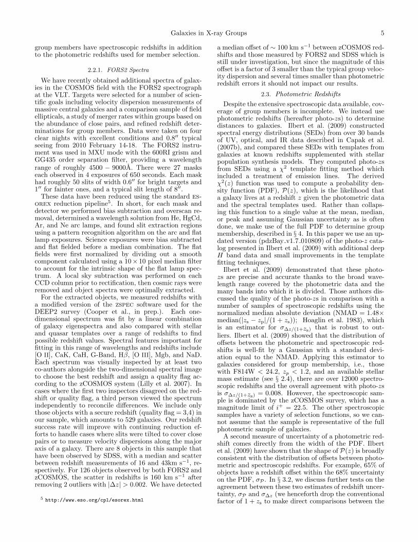
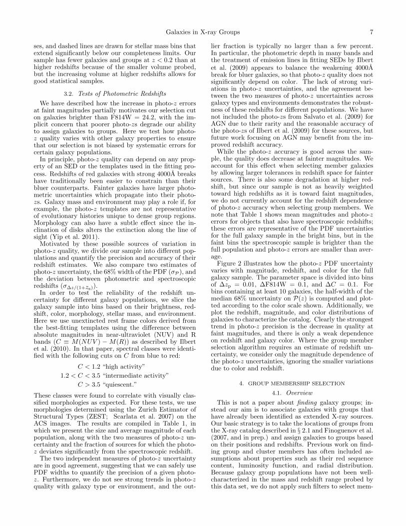
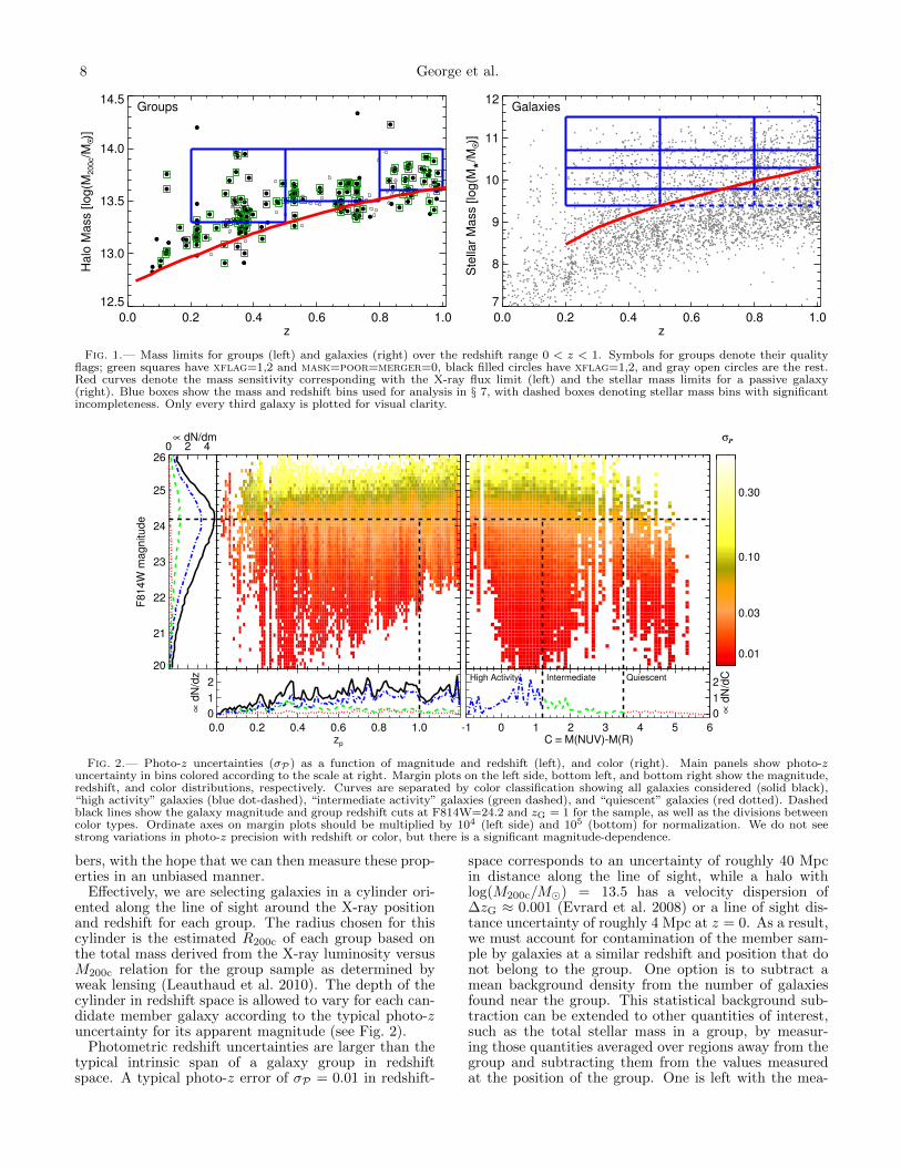
The left panel of Figure 1 shows the halo masses andredshifts for the group sample. Green squares representthe cleanest sample of 129 groups with xflag = 1 or 2,and none of the other flags set, black points relax therestrictions on the mask, poor, and merger flags, andgray dots represent the remaining sources in the catalogwith higher values of xflag. The red curve shows the 4σX-ray flux limit reached in 96% of the field of 1.0×10−15

erg cm−2 s−1 converted to a limiting group mass. Cov-erage is non-uniform, so some groups are detected belowthis threshold in areas with deeper coverage. Blue linesshow the mass and redshift bins used for later analysis.

To be considered for group membership and to de-rive stellar mass estimates, galaxies must be brighterthan F814W < 24.2 and have a photo-z in the range0 < zp < 1.2. Galaxies must also have a 3σ Ks-band detection, for which the typical limiting depth isKs = 24. Though the photometry in COSMOS is com-plete to i+ = 26.2 and has similar depths in other opti-cal filters (Capak et al. 2007b), the Ks-band detectionrequirement causes detections in the ACS imaging tobecome incomplete near F814W=24.2, which is also inthe magnitude range where photo-z quality deterioratesrapidly (see § 3.2). The F814W filter magnitude cor-relates more strongly with photo-z precision than longerwavelength filters (the 4000A break enters the filter rangeat z ∼ 0.75 and remains in that range beyond our red-shift limit), so we use it to apply the formal magnitudecut at F814W=24.2. Taking this as our primary mag-nitude cut, we find that only 5% of the sample withF814W < 24.2 is excluded due to a nondetection in Ks

or a failure to find an acceptable stellar mass fit, with 2%of bright objects (F814W < 22.5) and 8% of faint obects(23.5 < F814W < 24.2) being cut. Because of photo-zuncertainties, we allow galaxies to have a higher redshiftlimit than the groups in which they reside, giving thezp < 1.2 cut.

The right panel of Figure 1 shows the stellar massesand photometric redshifts for galaxies meeting the se-lection criteria. We plot only every third galaxy forclarity. The red curve shows the 85% stellar mass com-pleteness limit calculated for the oldest allowable stellartemplate at each redshift for the combined requirementsof Ks < 24 and F814W < 24.2. This passive limit isconservative, as younger stellar populations have lowermass-to-light ratios. At z = 1, our stellar mass limit isroughly log(M?/M) = 10.3, or 0.25M∗ (Drory et al.2009 found log(M∗/M) ≈ 10.9 for the massive end of adouble-Schechter function fit to the stellar mass functionat z ∼ 1, with little redshift evolution). Solid blue lines inthe figure show the mass and redshift bins for later analy-

Galaxies in X-ray Groups 7

ses, and dashed lines are drawn for stellar mass bins thatextend significantly below our completeness limits. Oursample has fewer galaxies and groups at z < 0.2 than athigher redshifts because of the smaller volume probed,but the increasing volume at higher redshifts allows forgood statistical samples.

3.2. Tests of Photometric Redshifts

We have described how the increase in photo-z errorsat faint magnitudes partially motivates our selection cuton galaxies brighter than F814W = 24.2, with the im-plicit concern that poorer photo-zs degrade our abilityto assign galaxies to groups. Here we test how photo-z quality varies with other galaxy properties to ensurethat our selection is not biased by systematic errors forcertain galaxy populations.

In principle, photo-z quality can depend on any prop-erty of an SED or the templates used in the fitting pro-cess. Redshifts of red galaxies with strong 4000A breakshave traditionally been easier to constrain than theirbluer counterparts. Fainter galaxies have larger photo-metric uncertainties which propagate into their photo-zs. Galaxy mass and environment may play a role if, forexample, the photo-z templates are not representativeof evolutionary histories unique to dense group regions.Morphology can also have a subtle effect since the in-clination of disks alters the extinction along the line ofsight (Yip et al. 2011).

Motivated by these possible sources of variation inphoto-z quality, we divide our sample into different pop-ulations and quantify the precision and accuracy of theirredshift estimates. We also compare two estimates ofphoto-z uncertainty, the 68% width of the PDF (σP), andthe deviation between photometric and spectroscopicredshifts (σ∆z/(1+zs)).

In order to test the reliability of the redshift un-certainty for different galaxy populations, we slice thegalaxy sample into bins based on their brightness, red-shift, color, morphology, stellar mass, and environment.Here we use unextincted rest frame colors derived fromthe best-fitting templates using the difference betweenabsolute magnitudes in near-ultraviolet (NUV) and Rbands (C ≡ M(NUV ) −M(R)) as described by Ilbertet al. (2010). In that paper, spectral classes were identi-fied with the following cuts on C from blue to red:

C < 1.2 “high activity”

1.2 < C < 3.5 “intermediate activity”

C > 3.5 “quiescent.”

These classes were found to correlate with visually clas-sified morphologies as expected. For these tests, we usemorphologies determined using the Zurich Estimator ofStructural Types (ZEST; Scarlata et al. 2007) on theACS images. The results are compiled in Table 1, inwhich we present the size and average magnitude of eachpopulation, along with the two measures of photo-z un-certainty and the fraction of sources for which the photo-z deviates significantly from the spectroscopic redshift.

The two independent measures of photo-z uncertaintyare in good agreement, suggesting that we can safely usePDF widths to quantify the precision of a given photo-z. Furthermore, we do not see strong trends in photo-zquality with galaxy type or environment, and the out-

lier fraction is typically no larger than a few percent.In particular, the photometric depth in many bands andthe treatment of emission lines in fitting SEDs by Ilbertet al. (2009) appears to balance the weakening 4000Abreak for bluer galaxies, so that photo-z quality does notsignificantly depend on color. The lack of strong vari-ations in photo-z uncertainties, and the agreement be-tween the two measures of photo-z uncertainties acrossgalaxy types and environments demonstrates the robust-ness of these redshifts for different populations. We havenot included the photo-zs from Salvato et al. (2009) forAGN due to their rarity and the reasonable accuracy ofthe photo-zs of Ilbert et al. (2009) for these sources, butfuture work focusing on AGN may benefit from the im-proved redshift accuracy.

While the photo-z accuracy is good across the sam-ple, the quality does decrease at fainter magnitudes. Weaccount for this effect when selecting member galaxiesby allowing larger tolerances in redshift space for faintersources. There is also some degradation at higher red-shift, but since our sample is not as heavily weightedtoward high redshifts as it is toward faint magnitudes,we do not currently account for the redshift dependenceof photo-z accuracy when selecting group members. Wenote that Table 1 shows mean magnitudes and photo-zerrors for objects that also have spectroscopic redshifts;these errors are representative of the PDF uncertaintiesfor the full galaxy sample in the bright bins, but in thefaint bins the spectroscopic sample is brighter than thefull population and photo-z errors are smaller than aver-age.

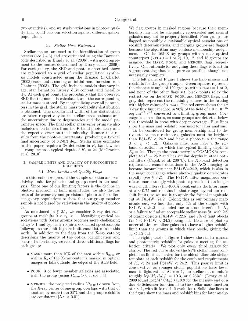
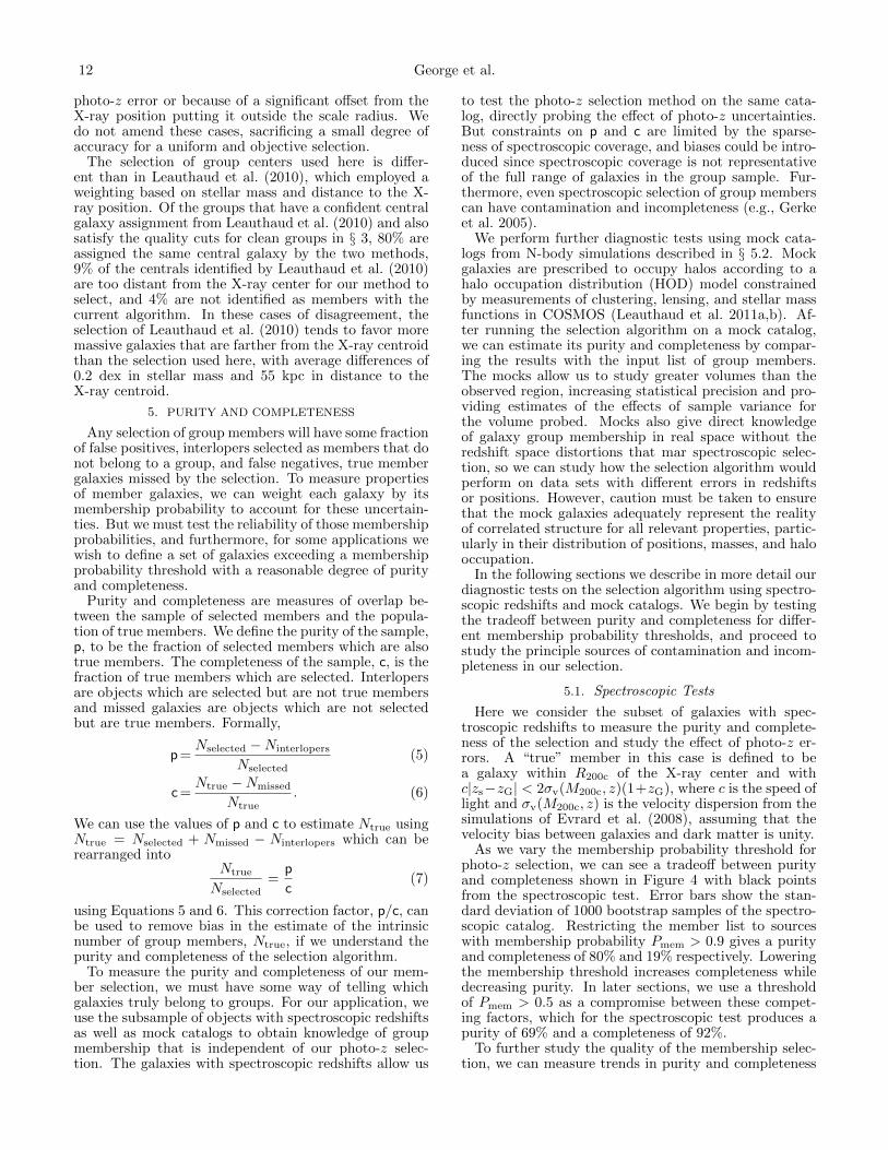
Figure 2 illustrates how the photo-z PDF uncertaintyvaries with magnitude, redshift, and color for the fullgalaxy sample. The parameter space is divided into binsof ∆zp = 0.01, ∆F814W = 0.1, and ∆C = 0.1. Forbins containing at least 10 galaxies, the half-width of themedian 68% uncertainty on P(z) is computed and plot-ted according to the color scale shown. Additionally, weplot the redshift, magnitude, and color distributions ofgalaxies to characterize the catalog. Clearly the strongesttrend in photo-z precision is the decrease in quality atfaint magnitudes, and there is only a weak dependenceon redshift and galaxy color. Where the group memberselection algorithm requires an estimate of redshift un-certainty, we consider only the magnitude dependence ofthe photo-z uncertainties, ignoring the smaller variationsdue to color and redshift.

4. GROUP MEMBERSHIP SELECTION

4.1. Overview

This is not a paper about finding galaxy groups; in-stead our aim is to associate galaxies with groups thathave already been identified as extended X-ray sources.Our basic strategy is to take the locations of groups fromthe X-ray catalog described in § 2.1 and Finoguenov et al.(2007, and in prep.) and assign galaxies to groups basedon their positions and redshifts. Previous work on find-ing group and cluster members has often included as-sumptions about properties such as their red sequencecontent, luminosity function, and radial distribution.Because galaxy group populations have not been well-characterized in the mass and redshift range probed bythis data set, we do not apply such filters to select mem-

8 George et al.

0.0 0.2 0.4 0.6 0.8 1.0z

12.5

13.0

13.5

14.0

14.5H

alo

Ma

ss [

log

(M200c/M

O •)]

Groups

0.0 0.2 0.4 0.6 0.8 1.0z

7

8

9

10

11

12

Ste

llar

Ma

ss [

log

(MH/M

O •)]

Galaxies

Fig. 1.— Mass limits for groups (left) and galaxies (right) over the redshift range 0 < z < 1. Symbols for groups denote their qualityflags; green squares have xflag=1,2 and mask=poor=merger=0, black filled circles have xflag=1,2, and gray open circles are the rest.Red curves denote the mass sensitivity corresponding with the X-ray flux limit (left) and the stellar mass limits for a passive galaxy(right). Blue boxes show the mass and redshift bins used for analysis in § 7, with dashed boxes denoting stellar mass bins with significantincompleteness. Only every third galaxy is plotted for visual clarity.

20

21

22

23

24

25

26

F8

14

W m

ag

nitu

de

0 2 4∝ dN/dm

0.0 0.2 0.4 0.6 0.8 1.0zp

0

1

2

∝ d

N/d

z

-1 0 1 2 3 4 5 6C ≡ M(NUV)-M(R)

0

1

2

∝ d

N/d

CHigh Activity Intermediate Quiescent

0.01

0.03

0.10

0.30

σP

Fig. 2.— Photo-z uncertainties (σP ) as a function of magnitude and redshift (left), and color (right). Main panels show photo-zuncertainty in bins colored according to the scale at right. Margin plots on the left side, bottom left, and bottom right show the magnitude,redshift, and color distributions, respectively. Curves are separated by color classification showing all galaxies considered (solid black),“high activity” galaxies (blue dot-dashed), “intermediate activity” galaxies (green dashed), and “quiescent” galaxies (red dotted). Dashedblack lines show the galaxy magnitude and group redshift cuts at F814W=24.2 and zG = 1 for the sample, as well as the divisions betweencolor types. Ordinate axes on margin plots should be multiplied by 104 (left side) and 105 (bottom) for normalization. We do not seestrong variations in photo-z precision with redshift or color, but there is a significant magnitude-dependence.

bers, with the hope that we can then measure these prop-erties in an unbiased manner.

Effectively, we are selecting galaxies in a cylinder ori-ented along the line of sight around the X-ray positionand redshift for each group. The radius chosen for thiscylinder is the estimated R200c of each group based onthe total mass derived from the X-ray luminosity versusM200c relation for the group sample as determined byweak lensing (Leauthaud et al. 2010). The depth of thecylinder in redshift space is allowed to vary for each can-didate member galaxy according to the typical photo-zuncertainty for its apparent magnitude (see Fig. 2).

Photometric redshift uncertainties are larger than thetypical intrinsic span of a galaxy group in redshiftspace. A typical photo-z error of σP = 0.01 in redshift-

space corresponds to an uncertainty of roughly 40 Mpcin distance along the line of sight, while a halo withlog(M200c/M) = 13.5 has a velocity dispersion of∆zG ≈ 0.001 (Evrard et al. 2008) or a line of sight dis-tance uncertainty of roughly 4 Mpc at z = 0. As a result,we must account for contamination of the member sam-ple by galaxies at a similar redshift and position that donot belong to the group. One option is to subtract amean background density from the number of galaxiesfound near the group. This statistical background sub-traction can be extended to other quantities of interest,such as the total stellar mass in a group, by measur-ing those quantities averaged over regions away from thegroup and subtracting them from the values measuredat the position of the group. One is left with the mea-

Galaxies in X-ray Groups 9

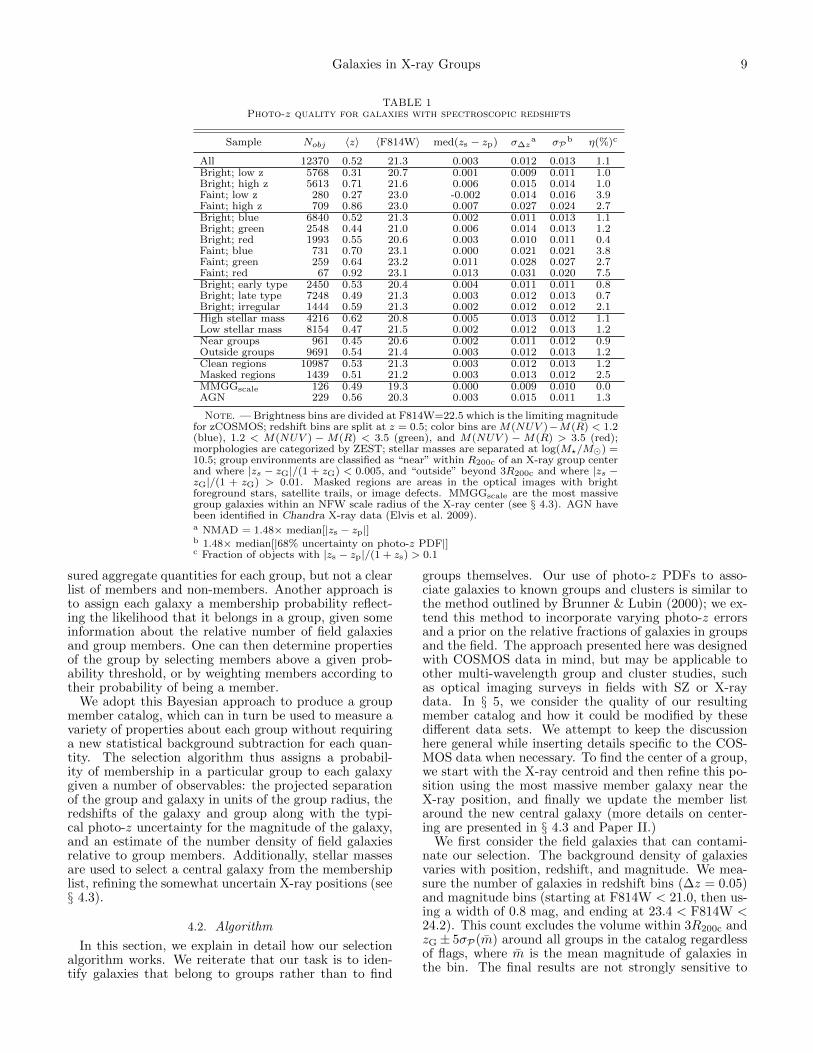
TABLE 1Photo-z quality for galaxies with spectroscopic redshifts

Sample Nobj 〈z〉 〈F814W〉 med(zs − zp) σ∆za σP

b η(%)c

All 12370 0.52 21.3 0.003 0.012 0.013 1.1Bright; low z 5768 0.31 20.7 0.001 0.009 0.011 1.0Bright; high z 5613 0.71 21.6 0.006 0.015 0.014 1.0Faint; low z 280 0.27 23.0 -0.002 0.014 0.016 3.9Faint; high z 709 0.86 23.0 0.007 0.027 0.024 2.7Bright; blue 6840 0.52 21.3 0.002 0.011 0.013 1.1Bright; green 2548 0.44 21.0 0.006 0.014 0.013 1.2Bright; red 1993 0.55 20.6 0.003 0.010 0.011 0.4Faint; blue 731 0.70 23.1 0.000 0.021 0.021 3.8Faint; green 259 0.64 23.2 0.011 0.028 0.027 2.7Faint; red 67 0.92 23.1 0.013 0.031 0.020 7.5Bright; early type 2450 0.53 20.4 0.004 0.011 0.011 0.8Bright; late type 7248 0.49 21.3 0.003 0.012 0.013 0.7Bright; irregular 1444 0.59 21.3 0.002 0.012 0.012 2.1High stellar mass 4216 0.62 20.8 0.005 0.013 0.012 1.1Low stellar mass 8154 0.47 21.5 0.002 0.012 0.013 1.2Near groups 961 0.45 20.6 0.002 0.011 0.012 0.9Outside groups 9691 0.54 21.4 0.003 0.012 0.013 1.2Clean regions 10987 0.53 21.3 0.003 0.012 0.013 1.2Masked regions 1439 0.51 21.2 0.003 0.013 0.012 2.5MMGGscale 126 0.49 19.3 0.000 0.009 0.010 0.0AGN 229 0.56 20.3 0.003 0.015 0.011 1.3

Note. — Brightness bins are divided at F814W=22.5 which is the limiting magnitudefor zCOSMOS; redshift bins are split at z = 0.5; color bins are M(NUV )−M(R) < 1.2(blue), 1.2 < M(NUV ) −M(R) < 3.5 (green), and M(NUV ) −M(R) > 3.5 (red);morphologies are categorized by ZEST; stellar masses are separated at log(M?/M) =10.5; group environments are classified as “near” within R200c of an X-ray group centerand where |zs − zG|/(1 + zG) < 0.005, and “outside” beyond 3R200c and where |zs −zG|/(1 + zG) > 0.01. Masked regions are areas in the optical images with brightforeground stars, satellite trails, or image defects. MMGGscale are the most massivegroup galaxies within an NFW scale radius of the X-ray center (see § 4.3). AGN havebeen identified in Chandra X-ray data (Elvis et al. 2009).a NMAD = 1.48× median[|zs − zp|]b 1.48× median[|68% uncertainty on photo-z PDF|]c Fraction of objects with |zs − zp|/(1 + zs) > 0.1

sured aggregate quantities for each group, but not a clearlist of members and non-members. Another approach isto assign each galaxy a membership probability reflect-ing the likelihood that it belongs in a group, given someinformation about the relative number of field galaxiesand group members. One can then determine propertiesof the group by selecting members above a given prob-ability threshold, or by weighting members according totheir probability of being a member.

We adopt this Bayesian approach to produce a groupmember catalog, which can in turn be used to measure avariety of properties about each group without requiringa new statistical background subtraction for each quan-tity. The selection algorithm thus assigns a probabil-ity of membership in a particular group to each galaxygiven a number of observables: the projected separationof the group and galaxy in units of the group radius, theredshifts of the galaxy and group along with the typi-cal photo-z uncertainty for the magnitude of the galaxy,and an estimate of the number density of field galaxiesrelative to group members. Additionally, stellar massesare used to select a central galaxy from the membershiplist, refining the somewhat uncertain X-ray positions (see§ 4.3).

4.2. Algorithm

In this section, we explain in detail how our selectionalgorithm works. We reiterate that our task is to iden-tify galaxies that belong to groups rather than to find

groups themselves. Our use of photo-z PDFs to asso-ciate galaxies to known groups and clusters is similar tothe method outlined by Brunner & Lubin (2000); we ex-tend this method to incorporate varying photo-z errorsand a prior on the relative fractions of galaxies in groupsand the field. The approach presented here was designedwith COSMOS data in mind, but may be applicable toother multi-wavelength group and cluster studies, suchas optical imaging surveys in fields with SZ or X-raydata. In § 5, we consider the quality of our resultingmember catalog and how it could be modified by thesedifferent data sets. We attempt to keep the discussionhere general while inserting details specific to the COS-MOS data when necessary. To find the center of a group,we start with the X-ray centroid and then refine this po-sition using the most massive member galaxy near theX-ray position, and finally we update the member listaround the new central galaxy (more details on center-ing are presented in § 4.3 and Paper II.)

We first consider the field galaxies that can contami-nate our selection. The background density of galaxiesvaries with position, redshift, and magnitude. We mea-sure the number of galaxies in redshift bins (∆z = 0.05)and magnitude bins (starting at F814W < 21.0, then us-ing a width of 0.8 mag, and ending at 23.4 < F814W <24.2). This count excludes the volume within 3R200c andzG ± 5σP(m) around all groups in the catalog regardlessof flags, where m is the mean magnitude of galaxies inthe bin. The final results are not strongly sensitive to

10 George et al.

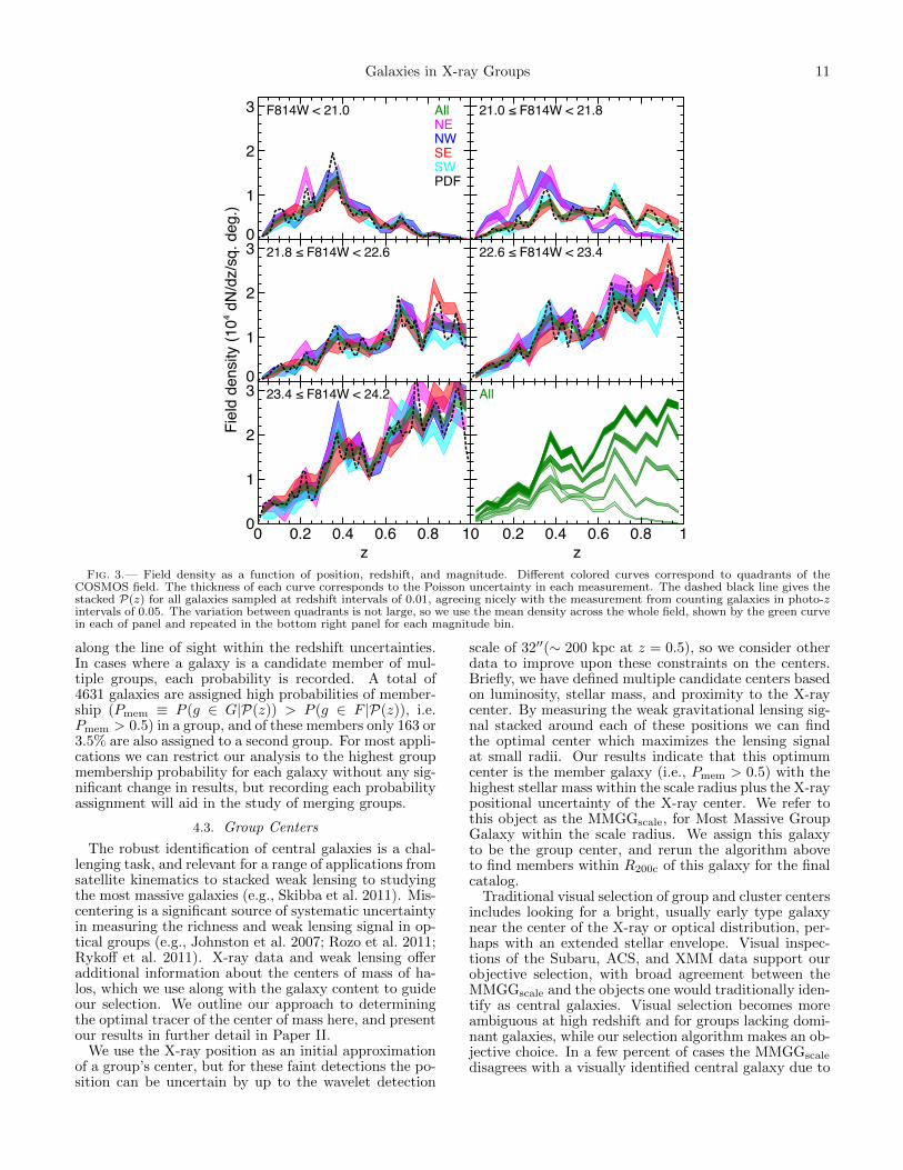
the choice of volume removed around groups. Figure 3shows this field density nF (F814W, z) = dNF/dz/dΩ,which is similar to the quantity shown in the bottom leftpanel of Figure 2 but split into magnitude bins. Figure 3also shows the field density as computed by summing theredshift probability distribution functions of galaxies forcomparison to the approach of directly counting galax-ies in photo-z bins. Despite different sampling intervals(∆z = 0.01 for the PDFs and 0.05 for bin counting), themethods show excellent agreement.

One can measure the background density locallyaround groups to account for correlated structure orglobally across the field to increase the statistical sam-ple with a larger volume, reducing noise. We have di-vided the COSMOS field into four separate quadrantsto look for variations in nF with position and find thatthe values are in reasonable agreement across the field,with the density in individual quandrants deviating fromthe mean by typically no more than the Poisson errors.When smaller volumes are chosen to estimate the fielddensity surrounding groups, the increased Poisson uncer-tainty swamps the constraint on locally correlated struc-ture. We thus opt to use the entire area to estimatethe mean density of background galaxies as a function ofmagnitude and redshift. We discuss further the choice ofthis method of estimating the field density in § 5.3.

We next consider candidate member galaxies, con-structing a list of those objects in a cylinder with a pro-jected distance from the group center less than R200c anda redshift within 3σP(mmax) of the group redshift zG,where mmax is the limiting magnitude F814W=24.2 andσP = 0.035. The number of member candidates can becompared with the field density in Figure 3 to estimatethe fraction of galaxies that are group members.

For each candidate, we compare the photo-z PDF tothe expected redshift distributions of group members andfield galaxies. We assume that each galaxy is either agroup member (G) or part of the field (F), and assign aBayesian membership probability using the relative sizesof the group and field populations as a prior to normal-ize the distributions. While the intial 3σP cut uses thephoto-z value zp to make a rough selection, here we usethe full distribution P(z) for each galaxy to account forsecondary peaks or other unusual features in the redshiftPDF. The probability that a galaxy belongs to a groupgiven P(z) can be written as

P (g ∈ G|P(z)) =P (P(z)|g ∈ G)P (g ∈ G)

P (P(z)). (1)

The term P (P(z)|g ∈ G) is the likelihood of measuringthe particular photo-z PDF for a known group member.The prior P (g ∈ G) = NG/(NG +NF ) = 1−P (g ∈ F ) isbased on the relative number of group and field galaxiesin the cylinder, and

P (P(z)) =P (P(z)|g ∈ G)P (g ∈ G) +

P (P(z)|g ∈ F )P (g ∈ F ) (2)

is the probability of measuring P(z) for any galaxy in thegroup or field. Each factor in Equation 1 has an implicitdependence on magnitude which we omit here and infollowing equations for notational simplicity, but we doaccount for magnitude-dependent variations in P(z) andin the field and group densities.

In order to compare the observed P(z) with that ex-pected for a group or field galaxy, we must assume adistribution of redshifts for each population. Since theintrinsic velocity dispersion of groups is smaller than theuncertainty in zp we model the true group redshift dis-tribution as a δ-function at zG, which is then convolvedwith a Gaussian of width σP(m) to account for photo-z measurement uncertainty. We have tested the effectsof modifying the true group redshift distribution to bebroader than a δ-function to account for intrinsic veloc-ity dispersion but found this correction to be negligible.The redshift distribution of field galaxies is assumed to beuniform near zG and remains unchanged after account-ing for photo-z measurement uncertainty. Each of theseredshift distributions is convolved with the photo-z PDFP(z) (note that

∫P(z)dz = 1), giving

P (P(z)|g ∈ G) =

∫P(z)N (zG, σP)dz (3)

P (P(z)|g ∈ F ) =

∫P(z)

w(σP)dz (4)

where N (zG, σP) is a Gaussian centered on the groupredshift with width equal to the typical P(z) uncertaintyfor the magnitude of the galaxy considered. The fielddensity distribution is normalized so that the integralover the redshift range zG ± 3σP is unity, so the widthnormalization parameter is w(σP(m)) = 6σP(m). Wehave written these convolutions as indefinite integrals,but in reality they are discrete sums sampled at the red-shift intervals ∆z = 0.01 and range 0 ≤ z ≤ 6 for whichP(z) has been calculated. Because P(z) is sampled atintervals close to the typical photo-z uncertainty, the dis-tribution can effectively become a δ-function, underesti-mating the true redshift error which has contributionsfrom template uncertainties as well as photometric un-certainties. So we first convolve P(z) with a Gaussian ofwidth dz = 0.01 to account for these uncertainties andavoid sharply peaked PDFs.

To estimate the prior, P (g ∈ G), we begin by countingthe number of galaxies in the range zG±3σP(m), measur-ing Ntot = NG +NF . The measurement of the field den-sity shown in Figure 3 provides an independent estimateof nF , which allows us to calculate an expected number offield galaxies in the cylinder, NF =

∫nF dzdΩ. For each

galaxy we linearly interpolate the curve in the relevantmagnitude bin to the group redshift, and multiply nF bythe volume searched around the group, 6πR200c

2σP(m),

to determine NF . This value is subtracted from the mea-sured Ntot to determine the expected number of groupgalaxies in the cylinder, NG. We use the estimated val-ues, NF and NG, to determine P (g ∈ G) and P (g ∈ F ),and Equation 1 assigns each galaxy a membership prob-ability between zero and one. In cases where a group isnot well-detected in a given magnitude bin (Ntot < NF ,

i.e. NG < 0), galaxies in the bin are flagged and ex-cluded from membership analysis. Tests in § 5 show thatexcluding these galaxies does not cause significant incom-pleteness in the member selection.

It is possible for the search cylinders of different groupsto overlap, either because they reside in neighboring po-sitions at the same redshift, or because of projections

Galaxies in X-ray Groups 11

PDF

All

NWNE

SWSE

F814W < 21.0

Fiel

d de

nsity

(104 d

N/dz

/sq.

deg

.)

0

1

2

3 21.0 ≤ F814W < 21.8

21.8 ≤ F814W < 22.6

0

1

2

3 22.6 ≤ F814W < 23.4

23.4 ≤ F814W < 24.2

0

1

2

3

z0 0.2 0.4 0.6 0.8 1

All

z0 0.2 0.4 0.6 0.8 1

Fig. 3.— Field density as a function of position, redshift, and magnitude. Different colored curves correspond to quadrants of theCOSMOS field. The thickness of each curve corresponds to the Poisson uncertainty in each measurement. The dashed black line gives thestacked P(z) for all galaxies sampled at redshift intervals of 0.01, agreeing nicely with the measurement from counting galaxies in photo-zintervals of 0.05. The variation between quadrants is not large, so we use the mean density across the whole field, shown by the green curvein each of panel and repeated in the bottom right panel for each magnitude bin.

along the line of sight within the redshift uncertainties.In cases where a galaxy is a candidate member of mul-tiple groups, each probability is recorded. A total of4631 galaxies are assigned high probabilities of member-ship (Pmem ≡ P (g ∈ G|P(z)) > P (g ∈ F |P(z)), i.e.Pmem > 0.5) in a group, and of these members only 163 or3.5% are also assigned to a second group. For most appli-cations we can restrict our analysis to the highest groupmembership probability for each galaxy without any sig-nificant change in results, but recording each probabilityassignment will aid in the study of merging groups.

4.3. Group Centers

The robust identification of central galaxies is a chal-lenging task, and relevant for a range of applications fromsatellite kinematics to stacked weak lensing to studyingthe most massive galaxies (e.g., Skibba et al. 2011). Mis-centering is a significant source of systematic uncertaintyin measuring the richness and weak lensing signal in op-tical groups (e.g., Johnston et al. 2007; Rozo et al. 2011;Rykoff et al. 2011). X-ray data and weak lensing offeradditional information about the centers of mass of ha-los, which we use along with the galaxy content to guideour selection. We outline our approach to determiningthe optimal tracer of the center of mass here, and presentour results in further detail in Paper II.

We use the X-ray position as an initial approximationof a group’s center, but for these faint detections the po-sition can be uncertain by up to the wavelet detection

scale of 32′′(∼ 200 kpc at z = 0.5), so we consider otherdata to improve upon these constraints on the centers.Briefly, we have defined multiple candidate centers basedon luminosity, stellar mass, and proximity to the X-raycenter. By measuring the weak gravitational lensing sig-nal stacked around each of these positions we can findthe optimal center which maximizes the lensing signalat small radii. Our results indicate that this optimumcenter is the member galaxy (i.e., Pmem > 0.5) with thehighest stellar mass within the scale radius plus the X-raypositional uncertainty of the X-ray center. We refer tothis object as the MMGGscale, for Most Massive GroupGalaxy within the scale radius. We assign this galaxyto be the group center, and rerun the algorithm aboveto find members within R200c of this galaxy for the finalcatalog.

Traditional visual selection of group and cluster centersincludes looking for a bright, usually early type galaxynear the center of the X-ray or optical distribution, per-haps with an extended stellar envelope. Visual inspec-tions of the Subaru, ACS, and XMM data support ourobjective selection, with broad agreement between theMMGGscale and the objects one would traditionally iden-tify as central galaxies. Visual selection becomes moreambiguous at high redshift and for groups lacking domi-nant galaxies, while our selection algorithm makes an ob-jective choice. In a few percent of cases the MMGGscale

disagrees with a visually identified central galaxy due to

12 George et al.

photo-z error or because of a significant offset from theX-ray position putting it outside the scale radius. Wedo not amend these cases, sacrificing a small degree ofaccuracy for a uniform and objective selection.

The selection of group centers used here is differ-ent than in Leauthaud et al. (2010), which employed aweighting based on stellar mass and distance to the X-ray position. Of the groups that have a confident centralgalaxy assignment from Leauthaud et al. (2010) and alsosatisfy the quality cuts for clean groups in § 3, 80% areassigned the same central galaxy by the two methods,9% of the centrals identified by Leauthaud et al. (2010)are too distant from the X-ray center for our method toselect, and 4% are not identified as members with thecurrent algorithm. In these cases of disagreement, theselection of Leauthaud et al. (2010) tends to favor moremassive galaxies that are farther from the X-ray centroidthan the selection used here, with average differences of0.2 dex in stellar mass and 55 kpc in distance to theX-ray centroid.

5. PURITY AND COMPLETENESS

Any selection of group members will have some fractionof false positives, interlopers selected as members that donot belong to a group, and false negatives, true membergalaxies missed by the selection. To measure propertiesof member galaxies, we can weight each galaxy by itsmembership probability to account for these uncertain-ties. But we must test the reliability of those membershipprobabilities, and furthermore, for some applications wewish to define a set of galaxies exceeding a membershipprobability threshold with a reasonable degree of purityand completeness.

Purity and completeness are measures of overlap be-tween the sample of selected members and the popula-tion of true members. We define the purity of the sample,p, to be the fraction of selected members which are alsotrue members. The completeness of the sample, c, is thefraction of true members which are selected. Interlopersare objects which are selected but are not true membersand missed galaxies are objects which are not selectedbut are true members. Formally,

p=Nselected −Ninterlopers

Nselected(5)

c=Ntrue −Nmissed

Ntrue. (6)

We can use the values of p and c to estimate Ntrue usingNtrue = Nselected + Nmissed − Ninterlopers which can berearranged into

Ntrue

Nselected=

p

c(7)

using Equations 5 and 6. This correction factor, p/c, canbe used to remove bias in the estimate of the intrinsicnumber of group members, Ntrue, if we understand thepurity and completeness of the selection algorithm.

To measure the purity and completeness of our mem-ber selection, we must have some way of telling whichgalaxies truly belong to groups. For our application, weuse the subsample of objects with spectroscopic redshiftsas well as mock catalogs to obtain knowledge of groupmembership that is independent of our photo-z selec-tion. The galaxies with spectroscopic redshifts allow us

to test the photo-z selection method on the same cata-log, directly probing the effect of photo-z uncertainties.But constraints on p and c are limited by the sparse-ness of spectroscopic coverage, and biases could be intro-duced since spectroscopic coverage is not representativeof the full range of galaxies in the group sample. Fur-thermore, even spectroscopic selection of group memberscan have contamination and incompleteness (e.g., Gerkeet al. 2005).

We perform further diagnostic tests using mock cata-logs from N-body simulations described in § 5.2. Mockgalaxies are prescribed to occupy halos according to ahalo occupation distribution (HOD) model constrainedby measurements of clustering, lensing, and stellar massfunctions in COSMOS (Leauthaud et al. 2011a,b). Af-ter running the selection algorithm on a mock catalog,we can estimate its purity and completeness by compar-ing the results with the input list of group members.The mocks allow us to study greater volumes than theobserved region, increasing statistical precision and pro-viding estimates of the effects of sample variance forthe volume probed. Mocks also give direct knowledgeof galaxy group membership in real space without theredshift space distortions that mar spectroscopic selec-tion, so we can study how the selection algorithm wouldperform on data sets with different errors in redshiftsor positions. However, caution must be taken to ensurethat the mock galaxies adequately represent the realityof correlated structure for all relevant properties, partic-ularly in their distribution of positions, masses, and halooccupation.

In the following sections we describe in more detail ourdiagnostic tests on the selection algorithm using spectro-scopic redshifts and mock catalogs. We begin by testingthe tradeoff between purity and completeness for differ-ent membership probability thresholds, and proceed tostudy the principle sources of contamination and incom-pleteness in our selection.

5.1. Spectroscopic Tests

Here we consider the subset of galaxies with spec-troscopic redshifts to measure the purity and complete-ness of the selection and study the effect of photo-z er-rors. A “true” member in this case is defined to bea galaxy within R200c of the X-ray center and withc|zs−zG| < 2σv(M200c, z)(1+zG), where c is the speed oflight and σv(M200c, z) is the velocity dispersion from thesimulations of Evrard et al. (2008), assuming that thevelocity bias between galaxies and dark matter is unity.

As we vary the membership probability threshold forphoto-z selection, we can see a tradeoff between purityand completeness shown in Figure 4 with black pointsfrom the spectroscopic test. Error bars show the stan-dard deviation of 1000 bootstrap samples of the spectro-scopic catalog. Restricting the member list to sourceswith membership probability Pmem > 0.9 gives a purityand completeness of 80% and 19% respectively. Loweringthe membership threshold increases completeness whiledecreasing purity. In later sections, we use a thresholdof Pmem > 0.5 as a compromise between these compet-ing factors, which for the spectroscopic test produces apurity of 69% and a completeness of 92%.

To further study the quality of the membership selec-tion, we can measure trends in purity and completeness

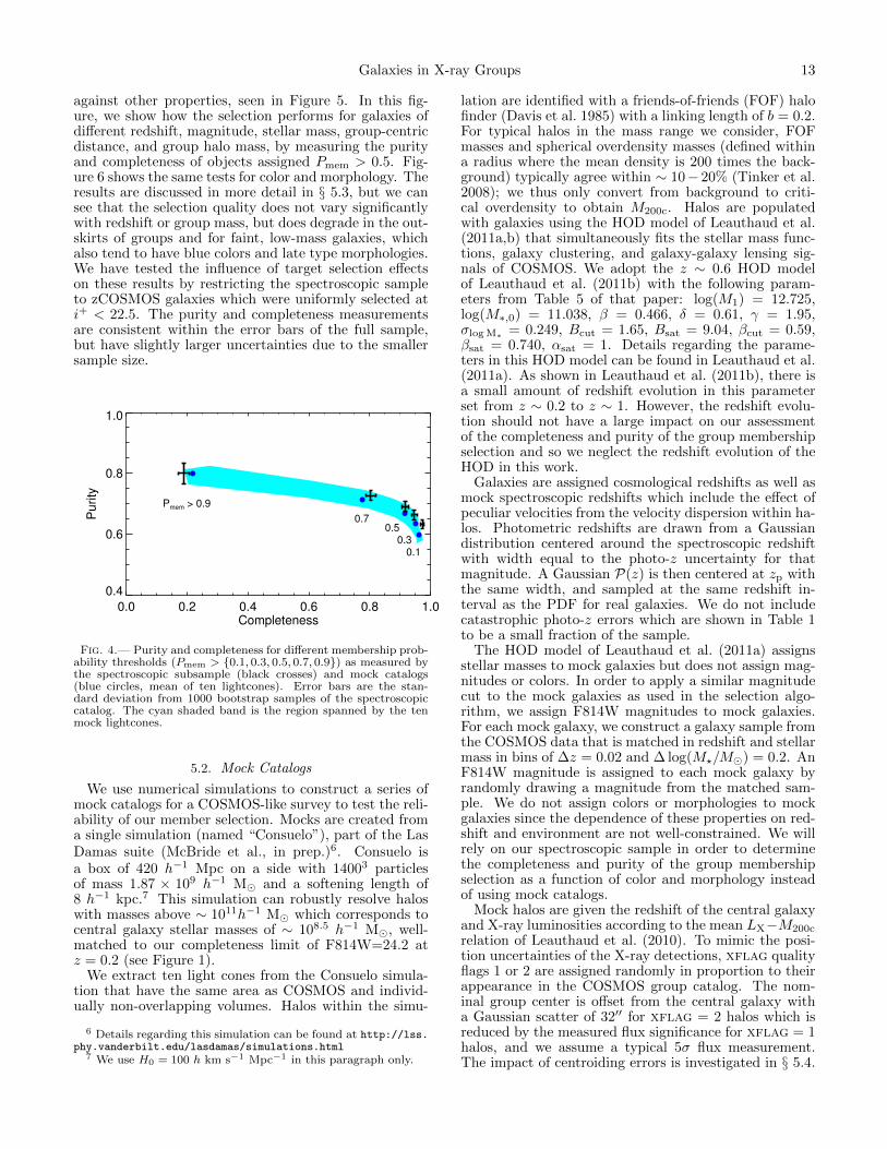
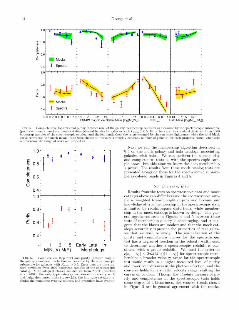
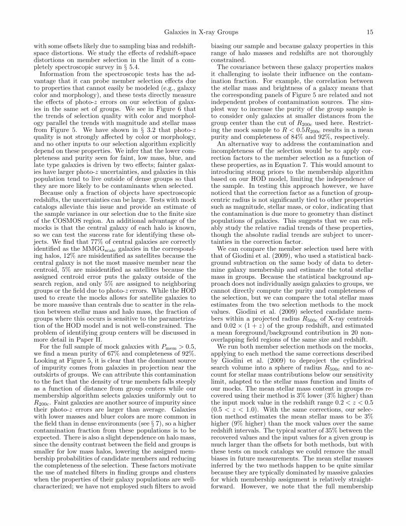
Galaxies in X-ray Groups 13

against other properties, seen in Figure 5. In this fig-ure, we show how the selection performs for galaxies ofdifferent redshift, magnitude, stellar mass, group-centricdistance, and group halo mass, by measuring the purityand completeness of objects assigned Pmem > 0.5. Fig-ure 6 shows the same tests for color and morphology. Theresults are discussed in more detail in § 5.3, but we cansee that the selection quality does not vary significantlywith redshift or group mass, but does degrade in the out-skirts of groups and for faint, low-mass galaxies, whichalso tend to have blue colors and late type morphologies.We have tested the influence of target selection effectson these results by restricting the spectroscopic sampleto zCOSMOS galaxies which were uniformly selected ati+ < 22.5. The purity and completeness measurementsare consistent within the error bars of the full sample,but have slightly larger uncertainties due to the smallersample size.

0.0 0.2 0.4 0.6 0.8 1.0Completeness

0.4

0.6

0.8

1.0

Purity

Pmem > 0.9

0.70.5

0.30.1

Fig. 4.— Purity and completeness for different membership prob-ability thresholds (Pmem > 0.1, 0.3, 0.5, 0.7, 0.9) as measured bythe spectroscopic subsample (black crosses) and mock catalogs(blue circles, mean of ten lightcones). Error bars are the stan-dard deviation from 1000 bootstrap samples of the spectroscopiccatalog. The cyan shaded band is the region spanned by the tenmock lightcones.

5.2. Mock Catalogs

We use numerical simulations to construct a series ofmock catalogs for a COSMOS-like survey to test the reli-ability of our member selection. Mocks are created froma single simulation (named “Consuelo”), part of the LasDamas suite (McBride et al., in prep.)6. Consuelo isa box of 420 h−1 Mpc on a side with 14003 particlesof mass 1.87 × 109 h−1 M and a softening length of8 h−1 kpc.7 This simulation can robustly resolve haloswith masses above ∼ 1011h−1 M which corresponds tocentral galaxy stellar masses of ∼ 108.5 h−1 M, well-matched to our completeness limit of F814W=24.2 atz = 0.2 (see Figure 1).

We extract ten light cones from the Consuelo simula-tion that have the same area as COSMOS and individ-ually non-overlapping volumes. Halos within the simu-

6 Details regarding this simulation can be found at http://lss.phy.vanderbilt.edu/lasdamas/simulations.html

7 We use H0 = 100 h km s−1 Mpc−1 in this paragraph only.

lation are identified with a friends-of-friends (FOF) halofinder (Davis et al. 1985) with a linking length of b = 0.2.For typical halos in the mass range we consider, FOFmasses and spherical overdensity masses (defined withina radius where the mean density is 200 times the back-ground) typically agree within ∼ 10− 20% (Tinker et al.2008); we thus only convert from background to criti-cal overdensity to obtain M200c. Halos are populatedwith galaxies using the HOD model of Leauthaud et al.(2011a,b) that simultaneously fits the stellar mass func-tions, galaxy clustering, and galaxy-galaxy lensing sig-nals of COSMOS. We adopt the z ∼ 0.6 HOD modelof Leauthaud et al. (2011b) with the following param-eters from Table 5 of that paper: log(M1) = 12.725,log(M∗,0) = 11.038, β = 0.466, δ = 0.61, γ = 1.95,σlog M∗ = 0.249, Bcut = 1.65, Bsat = 9.04, βcut = 0.59,βsat = 0.740, αsat = 1. Details regarding the parame-ters in this HOD model can be found in Leauthaud et al.(2011a). As shown in Leauthaud et al. (2011b), there isa small amount of redshift evolution in this parameterset from z ∼ 0.2 to z ∼ 1. However, the redshift evolu-tion should not have a large impact on our assessmentof the completeness and purity of the group membershipselection and so we neglect the redshift evolution of theHOD in this work.

Galaxies are assigned cosmological redshifts as well asmock spectroscopic redshifts which include the effect ofpeculiar velocities from the velocity dispersion within ha-los. Photometric redshifts are drawn from a Gaussiandistribution centered around the spectroscopic redshiftwith width equal to the photo-z uncertainty for thatmagnitude. A Gaussian P(z) is then centered at zp withthe same width, and sampled at the same redshift in-terval as the PDF for real galaxies. We do not includecatastrophic photo-z errors which are shown in Table 1to be a small fraction of the sample.

The HOD model of Leauthaud et al. (2011a) assignsstellar masses to mock galaxies but does not assign mag-nitudes or colors. In order to apply a similar magnitudecut to the mock galaxies as used in the selection algo-rithm, we assign F814W magnitudes to mock galaxies.For each mock galaxy, we construct a galaxy sample fromthe COSMOS data that is matched in redshift and stellarmass in bins of ∆z = 0.02 and ∆ log(M?/M) = 0.2. AnF814W magnitude is assigned to each mock galaxy byrandomly drawing a magnitude from the matched sam-ple. We do not assign colors or morphologies to mockgalaxies since the dependence of these properties on red-shift and environment are not well-constrained. We willrely on our spectroscopic sample in order to determinethe completeness and purity of the group membershipselection as a function of color and morphology insteadof using mock catalogs.

Mock halos are given the redshift of the central galaxyand X-ray luminosities according to the mean LX−M200c

relation of Leauthaud et al. (2010). To mimic the posi-tion uncertainties of the X-ray detections, xflag qualityflags 1 or 2 are assigned randomly in proportion to theirappearance in the COSMOS group catalog. The nom-inal group center is offset from the central galaxy witha Gaussian scatter of 32′′ for xflag = 2 halos which isreduced by the measured flux significance for xflag = 1halos, and we assume a typical 5σ flux measurement.The impact of centroiding errors is investigated in § 5.4.

14 George et al.

0.0 0.2 0.4 0.6 0.8 1.0z

0.4

0.6

0.8

1.0

Pu

rity

Mocks

Spectra

18 20 22 24F814W magnitude

9 10 11Stellar Mass [log(M

/M

O •)]

0.0 0.2 0.4 0.6 0.8 1.0R/R200c

13.0 13.5 14.0Halo Mass [log(M200c/MO •

)]

0.4

0.6

0.8

1.0

Co

mp

lete

ne

ss

Mocks

Spectra

Fig. 5.— Completeness (top row) and purity (bottom row) of the galaxy membership selection as measured by the spectroscopic subsample(points with error bars) and mock catalogs (shaded bands) for galaxies with Pmem > 0.5. Error bars are the standard deviation from 1000bootstrap samples of the spectroscopic catalog, and shaded bands show the range spanned by the ten mock lightcones, while the solid blackcurve represents the mock mean. Bins were chosen to measure a roughly constant number of galaxies for each property tested while stillrepresenting the range of observed properties.

-1 1 3 5M(NUV)-M(R)

0.4

0.6

0.8

1.0

Purity

Early Late IrrMorphology

0.4

0.6

0.8

1.0

Com

ple

teness

Fig. 6.— Completeness (top row) and purity (bottom row) ofthe galaxy membership selection as measured by the spectroscopicsubsample for galaxies with Pmem > 0.5. Error bars are the stan-dard deviation from 1000 bootstrap samples of the spectroscopiccatalog. Morphological classes are defined from ZEST (Scarlataet al. 2007); the early type category includes ellipticals (type=1)and bulge-dominated disks (type=2.0), the late type category in-cludes the remaining type=2 sources, and irregulars have type=3.

Next we run the membership algorithm described in§ 4 on the mock galaxy and halo catalogs, associatinggalaxies with halos. We can perform the same purityand completeness tests as with the spectroscopic sam-ple above, but this time we know the halo membershipa priori. The results from these mock catalog tests arepresented alongside those for the spectroscopic subsam-ple as colored bands in Figures 4 and 5.

5.3. Sources of Error

Results from the tests on spectroscopic data and mockcatalogs above can differ because the spectroscopic sam-ple is weighted toward bright objects and because ourknowledge of true membership in the spectroscopic datais limited by redshift-space distortions, while member-ship in the mock catalogs is known by design. The gen-eral agreement seen in Figures 4 and 5 between thesetests of membership quality is encouraging, and it sug-gests that the biases are modest and that the mock cat-alogs accurately represent the properties of real galax-ies that we wish to study. The normalization of thepurity and completeness curves for the spectroscopictest has a degree of freedom in the velocity width usedto determine whether a spectroscopic redshift is con-sistent with a group redshift. We used the criterionc|zs − zG| < 2σv(M, z)(1 + zG) for spectroscopic mem-bership; a broader velocity range for the spectroscopictest would result in a higher measured level of purityand lower completeness in the photo-z selection, and theconverse holds for a smaller velocity range, shifting thecurves up or down. Though the absolute measure of pu-rity and completeness in the spectroscopic tests holdssome degree of arbitrariness, the relative trends shownin Figure 5 are in general agreement with the mocks,

Galaxies in X-ray Groups 15

with some offsets likely due to sampling bias and redshift-space distortions. We study the effects of redshift-spacedistortions on member selection in the limit of a com-pletely spectroscopic survey in § 5.4.

Information from the spectroscopic tests has the ad-vantage that it can probe member selection effects dueto properties that cannot easily be modeled (e.g., galaxycolor and morphology), and these tests directly measurethe effects of photo-z errors on our selection of galax-ies in the same set of groups. We see in Figure 6 thatthe trends of selection quality with color and morphol-ogy parallel the trends with magnitude and stellar massfrom Figure 5. We have shown in § 3.2 that photo-zquality is not strongly affected by color or morphology,and no other inputs to our selection algorithm explicitlydepend on these properties. We infer that the lower com-pleteness and purity seen for faint, low mass, blue, andlate type galaxies is driven by two effects; fainter galax-ies have larger photo-z uncertainties, and galaxies in thispopulation tend to live outside of dense groups so thatthey are more likely to be contaminants when selected.

Because only a fraction of objects have spectroscopicredshifts, the uncertainties can be large. Tests with mockcatalogs alleviate this issue and provide an estimate ofthe sample variance in our selection due to the finite sizeof the COSMOS region. An additional advantage of themocks is that the central galaxy of each halo is known,so we can test the success rate for identifying these ob-jects. We find that 77% of central galaxies are correctlyidentified as the MMGGscale galaxies in the correspond-ing halos, 12% are misidentified as satellites because thecentral galaxy is not the most massive member near thecentroid, 5% are misidentified as satellites because theassigned centroid error puts the galaxy outside of thesearch region, and only 5% are assigned to neighboringgroups or the field due to photo-z errors. While the HODused to create the mocks allows for satellite galaxies tobe more massive than centrals due to scatter in the rela-tion between stellar mass and halo mass, the fraction ofgroups where this occurs is sensitive to the parametriza-tion of the HOD model and is not well-constrained. Theproblem of identifying group centers will be discussed inmore detail in Paper II.

For the full sample of mock galaxies with Pmem > 0.5,we find a mean purity of 67% and completeness of 92%.Looking at Figure 5, it is clear that the dominant sourceof impurity comes from galaxies in projection near theoutskirts of groups. We can attribute this contaminationto the fact that the density of true members falls steeplyas a function of distance from group centers while ourmembership algorithm selects galaxies uniformly out toR200c. Faint galaxies are another source of impurity sincetheir photo-z errors are larger than average. Galaxieswith lower masses and bluer colors are more common inthe field than in dense environments (see § 7), so a highercontamination fraction from these populations is to beexpected. There is also a slight dependence on halo mass,since the density contrast between the field and groups issmaller for low mass halos, lowering the assigned mem-bership probabilities of candidate members and reducingthe completeness of the selection. These factors motivatethe use of matched filters in finding groups and clusterswhen the properties of their galaxy populations are well-characterized; we have not employed such filters to avoid

biasing our sample and because galaxy properties in thisrange of halo masses and redshifts are not thoroughlyconstrained.

The covariance between these galaxy properties makesit challenging to isolate their influence on the contam-ination fraction. For example, the correlation betweenthe stellar mass and brightness of a galaxy means thatthe corresponding panels of Figure 5 are related and notindependent probes of contamination sources. The sim-plest way to increase the purity of the group sample isto consider only galaxies at smaller distances from thegroup center than the cut of R200c used here. Restrict-ing the mock sample to R < 0.5R200c results in a meanpurity and completeness of 84% and 92%, respectively.

An alternative way to address the contamination andincompleteness of the selection would be to apply cor-rection factors to the member selection as a function ofthese properties, as in Equation 7. This would amount tointroducing strong priors to the membership algorithmbased on our HOD model, limiting the independence ofthe sample. In testing this approach however, we havenoticed that the correction factor as a function of group-centric radius is not significantly tied to other propertiessuch as magnitude, stellar mass, or color, indicating thatthe contamination is due more to geometry than distinctpopulations of galaxies. This suggests that we can reli-ably study the relative radial trends of these properties,though the absolute radial trends are subject to uncer-tainties in the correction factor.

We can compare the member selection used here withthat of Giodini et al. (2009), who used a statistical back-ground subtraction on the same body of data to deter-mine galaxy membership and estimate the total stellarmass in groups. Because the statistical background ap-proach does not individually assign galaxies to groups, wecannot directly compute the purity and completeness ofthe selection, but we can compare the total stellar massestimates from the two selection methods to the mockvalues. Giodini et al. (2009) selected candidate mem-bers within a projected radius R500c of X-ray centroidsand 0.02 × (1 + z) of the group redshift, and estimateda mean foreground/background contribution in 20 non-overlapping field regions of the same size and redshift.

We run both member selection methods on the mocks,applying to each method the same corrections describedby Giodini et al. (2009) to deproject the cylindricalsearch volume into a sphere of radius R500c and to ac-count for stellar mass contributions below our sensitivitylimit, adapted to the stellar mass function and limits ofour mocks. The mean stellar mass content in groups re-covered using their method is 3% lower (3% higher) thanthe input mock value in the redshift range 0.2 < z < 0.5(0.5 < z < 1.0). With the same corrections, our selec-tion method estimates the mean stellar mass to be 3%higher (9% higher) than the mock values over the sameredshift intervals. The typical scatter of 35% between therecovered values and the input values for a given group ismuch larger than the offsets for both methods, but withthese tests on mock catalogs we could remove the smallbiases in future measurements. The mean stellar massesinferred by the two methods happen to be quite similarbecause they are typically dominated by massive galaxiesfor which membership assignment is relatively straight-forward. However, we note that the full membership

16 George et al.

selected can be quite different because our approach op-timizes group centers using the weak lensing signal andhandles magnitude-dependent photometric redshift un-certainties, whereas Giodini et al. (2009) use the X-raycenters and a fixed redshift window.

We can also test different methods of estimating thefield density to see how it influences our member selec-tion. Our selection algorithm estimates NF from themean density across the whole field, but smaller re-gions could instead be used to estimate the local densityaround individual groups. While the local density esti-mate has the advantage that it traces correlated struc-ture around groups, it does suffer from greater shot noisethan the density estimated over a larger volume. Wehave tested our approach by using annuli centered oneach group with inner and outer radii of 2R200c and5R200c, while keeping the rest of the selection algorithmthe same. With this approach, the typical field densityis higher due to clustering around groups and the result-ing membership probability is slightly lower (increasingthe field density by a factor of 2 typically lowers themembership probability by only ∼ 20%), but the pu-rity and completeness of the sample are essentially un-changed, and the fraction of members crossing a thresh-old of Pmem > 0.5 between samples is less than 10%.We obtain similar results when substituting the back-ground estimation method used by Giodini et al. (2009)for our field density prior, so the selection algorithm isnot strongly sensitive to the approach used for back-ground estimation.

5.4. Applicability to Other Surveys

In view of other surveys which will search for groupsand clusters in multi-wavelength data, and to bettercharacterize the advantages or shortcomings of the COS-MOS data used in this analysis, we test our selectionalgorithm on mock catalogs with different levels of un-certainty in redshift and centroid measurements. Weconsider five hypothetical data sets: a full spectroscopicsurvey where all galaxies have the typical redshift uncer-tainty in zCOSMOS8 of σz = 3.7×10−4, a low-resolutionspectroscopic survey like PRIMUS (Coil et al. 2010) withredshift uncertainties of σz = 0.005, a photometric sur-vey with fewer bands and larger photo-z errors like SDSS(Csabai et al. 2003) or DES (Banerji et al. 2008) withσz = 0.05, a deeper X-ray survey with more precise cen-troids of 3′′, and a lower resolution X-ray or SZ surveywith centroid uncertainties of 1′. In the first three mocksurveys we vary only the redshift uncertainty and ap-ply the same centering uncertainty as the fiducial COS-MOS mocks described in § 5.2 assuming similar X-raydetections. In the final two mock surveys we use themagnitude-dependent redshift uncertainties of the COS-MOS mocks and assign centroiding uncertainties, σX, ineach dimension on the sky. We offset the nominal cen-troid from the central galaxy in each dimension by arandom value drawn from a Gaussian of width σX. Inall cases we keep the same group and galaxy detectionlimits as in the COSMOS data.

Figures 7 and 8 show the purity and completeness ob-tained when applying our member selection algorithm to

8 http://archive.eso.org/archive/adp/zCOSMOS/VIMOS_spectroscopy_v1.0/index.html

these mock surveys, in a manner similar to Figure 5. Wereiterate that these statistics describe the accuracy of theassignment of galaxies to groups, and not the detectionof groups themselves. The figure illustrates that purityand completeness improve as redshift and centroid uncer-tainties decline. A number of other points can be madeabout these results:

• Deeper and more complete spectroscopic coveragewould improve our member selection, increasingthe purity of the sample from ∼ 70% with photo-zsto ∼ 85%. Improvements for completeness wouldmainly be gained from faint galaxies near our mag-nitude limit.

• Among spectroscopic redshifts, high precision isnot critical. The completeness of the σz =3.7 × 10−4 and 0.005 samples are nearly identi-cal, and the higher precision spectra provide onlya modest improvement in sample purity over thelow-resolution spectra, from ∼ 80% to ∼ 85%.Once the redshift measurement uncertainty be-comes comparable to the magnitude of intrin-sic redshift distortions due to peculiar velocitiesin groups, additional spectral resolution does notgreatly improve our ability to identify members.PRIMUS data in the COSMOS field will improveupon the existing sampling of zCOSMOS, but wenote that the completeness limit for that survey isi = 22.5 with sparse sampling to i = 23.5, stillshallower than our photo-z depth of F814W=24.2.

• The precise photometric redshifts available in theCOSMOS field are critical for identifying membersusing our approach. Redshifts that are less accu-rate or precise show significantly reduced purityand completeness.

• The precision of X-ray centroids for COSMOSgroups is quite sufficient for member selection. Im-proving the positional uncertainty by roughly a fac-tor of eight from the mean COSMOS value resultsin only a few percent improvement in completenessand a negligible gain in purity. Conversely, less pre-cise centers (such as those available from SZ mea-surements) produce a sample with lower purity inthe central region (∼ 85% instead of ∼ 95%) andsignificantly lower completeness (∼ 75% insteadof ∼ 90%). Though the existing COSMOS cen-troids are adequate for assigning member galaxiesto groups, we note that several aspects of groupscould still be studied with deeper X-ray or SZ dataincluding physical offsets between central galaxiesand hot gas, and the relationships between temper-ature or entropy with other group properties.

• Note that we do not optimize our selection algo-rithm for these hypothetical data sets. Combin-ing catalogs built from different observables (e.g.,Cohn & White 2009), and other techniques such asiterative centering or matched filters could improveresults.

We can compare the results of our mock spectroscopicselection to other methods in the literature. We must

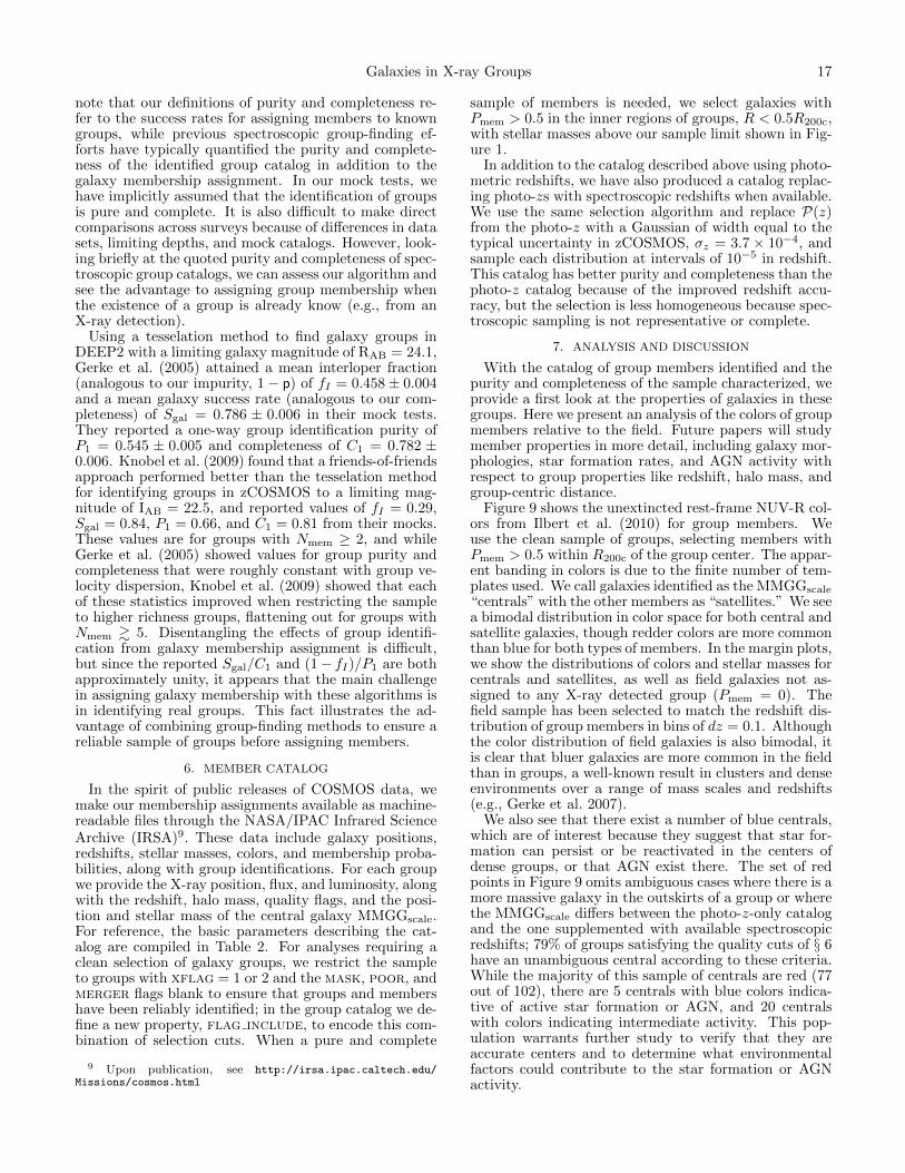
Galaxies in X-ray Groups 17

note that our definitions of purity and completeness re-fer to the success rates for assigning members to knowngroups, while previous spectroscopic group-finding ef-forts have typically quantified the purity and complete-ness of the identified group catalog in addition to thegalaxy membership assignment. In our mock tests, wehave implicitly assumed that the identification of groupsis pure and complete. It is also difficult to make directcomparisons across surveys because of differences in datasets, limiting depths, and mock catalogs. However, look-ing briefly at the quoted purity and completeness of spec-troscopic group catalogs, we can assess our algorithm andsee the advantage to assigning group membership whenthe existence of a group is already know (e.g., from anX-ray detection).

Using a tesselation method to find galaxy groups inDEEP2 with a limiting galaxy magnitude of RAB = 24.1,Gerke et al. (2005) attained a mean interloper fraction(analogous to our impurity, 1− p) of fI = 0.458± 0.004and a mean galaxy success rate (analogous to our com-pleteness) of Sgal = 0.786 ± 0.006 in their mock tests.They reported a one-way group identification purity ofP1 = 0.545 ± 0.005 and completeness of C1 = 0.782 ±0.006. Knobel et al. (2009) found that a friends-of-friendsapproach performed better than the tesselation methodfor identifying groups in zCOSMOS to a limiting mag-nitude of IAB = 22.5, and reported values of fI = 0.29,Sgal = 0.84, P1 = 0.66, and C1 = 0.81 from their mocks.These values are for groups with Nmem ≥ 2, and whileGerke et al. (2005) showed values for group purity andcompleteness that were roughly constant with group ve-locity dispersion, Knobel et al. (2009) showed that eachof these statistics improved when restricting the sampleto higher richness groups, flattening out for groups withNmem & 5. Disentangling the effects of group identifi-cation from galaxy membership assignment is difficult,but since the reported Sgal/C1 and (1− fI)/P1 are bothapproximately unity, it appears that the main challengein assigning galaxy membership with these algorithms isin identifying real groups. This fact illustrates the ad-vantage of combining group-finding methods to ensure areliable sample of groups before assigning members.

6. MEMBER CATALOG

In the spirit of public releases of COSMOS data, wemake our membership assignments available as machine-readable files through the NASA/IPAC Infrared ScienceArchive (IRSA)9. These data include galaxy positions,redshifts, stellar masses, colors, and membership proba-bilities, along with group identifications. For each groupwe provide the X-ray position, flux, and luminosity, alongwith the redshift, halo mass, quality flags, and the posi-tion and stellar mass of the central galaxy MMGGscale.For reference, the basic parameters describing the cat-alog are compiled in Table 2. For analyses requiring aclean selection of galaxy groups, we restrict the sampleto groups with xflag = 1 or 2 and the mask, poor, andmerger flags blank to ensure that groups and membershave been reliably identified; in the group catalog we de-fine a new property, flag include, to encode this com-bination of selection cuts. When a pure and complete

9 Upon publication, see http://irsa.ipac.caltech.edu/Missions/cosmos.html

sample of members is needed, we select galaxies withPmem > 0.5 in the inner regions of groups, R < 0.5R200c,with stellar masses above our sample limit shown in Fig-ure 1.

In addition to the catalog described above using photo-metric redshifts, we have also produced a catalog replac-ing photo-zs with spectroscopic redshifts when available.We use the same selection algorithm and replace P(z)from the photo-z with a Gaussian of width equal to thetypical uncertainty in zCOSMOS, σz = 3.7 × 10−4, andsample each distribution at intervals of 10−5 in redshift.This catalog has better purity and completeness than thephoto-z catalog because of the improved redshift accu-racy, but the selection is less homogeneous because spec-troscopic sampling is not representative or complete.

7. ANALYSIS AND DISCUSSION

With the catalog of group members identified and thepurity and completeness of the sample characterized, weprovide a first look at the properties of galaxies in thesegroups. Here we present an analysis of the colors of groupmembers relative to the field. Future papers will studymember properties in more detail, including galaxy mor-phologies, star formation rates, and AGN activity withrespect to group properties like redshift, halo mass, andgroup-centric distance.

Figure 9 shows the unextincted rest-frame NUV-R col-ors from Ilbert et al. (2010) for group members. Weuse the clean sample of groups, selecting members withPmem > 0.5 within R200c of the group center. The appar-ent banding in colors is due to the finite number of tem-plates used. We call galaxies identified as the MMGGscale

“centrals” with the other members as “satellites.” We seea bimodal distribution in color space for both central andsatellite galaxies, though redder colors are more commonthan blue for both types of members. In the margin plots,we show the distributions of colors and stellar masses forcentrals and satellites, as well as field galaxies not as-signed to any X-ray detected group (Pmem = 0). Thefield sample has been selected to match the redshift dis-tribution of group members in bins of dz = 0.1. Althoughthe color distribution of field galaxies is also bimodal, itis clear that bluer galaxies are more common in the fieldthan in groups, a well-known result in clusters and denseenvironments over a range of mass scales and redshifts(e.g., Gerke et al. 2007).

We also see that there exist a number of blue centrals,which are of interest because they suggest that star for-mation can persist or be reactivated in the centers ofdense groups, or that AGN exist there. The set of redpoints in Figure 9 omits ambiguous cases where there is amore massive galaxy in the outskirts of a group or wherethe MMGGscale differs between the photo-z-only catalogand the one supplemented with available spectroscopicredshifts; 79% of groups satisfying the quality cuts of § 6have an unambiguous central according to these criteria.While the majority of this sample of centrals are red (77out of 102), there are 5 centrals with blue colors indica-tive of active star formation or AGN, and 20 centralswith colors indicating intermediate activity. This pop-ulation warrants further study to verify that they areaccurate centers and to determine what environmentalfactors could contribute to the star formation or AGNactivity.

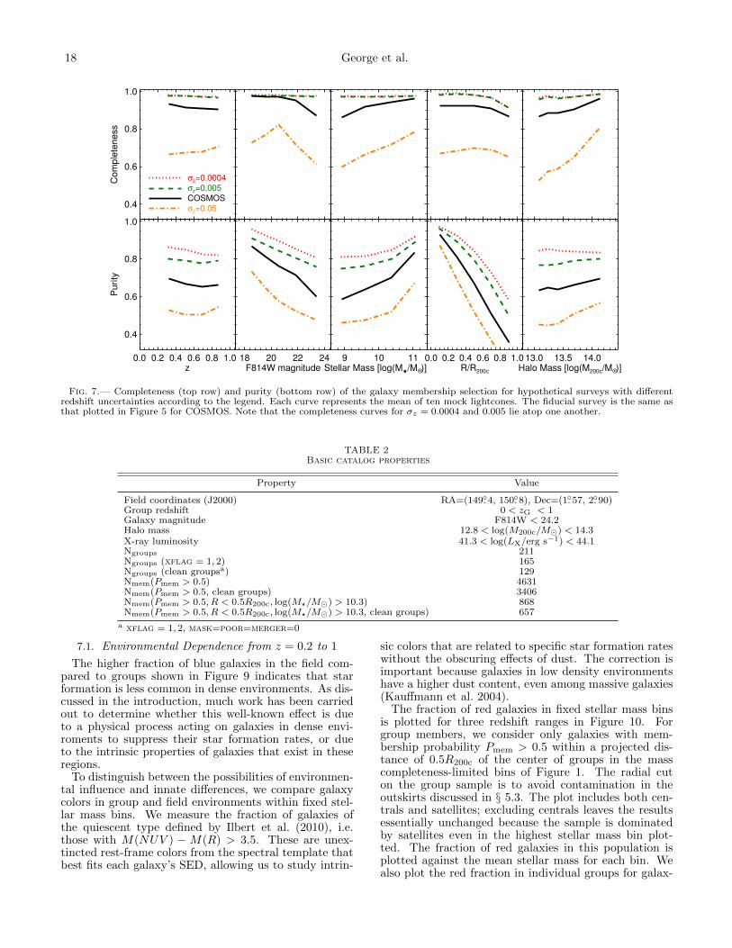
18 George et al.

0.0 0.2 0.4 0.6 0.8 1.0z

0.4

0.6

0.8

1.0

Pu

rity

18 20 22 24F814W magnitude

9 10 11Stellar Mass [log(M

H/M

O •)]

0.0 0.2 0.4 0.6 0.8 1.0R/R200c

13.0 13.5 14.0Halo Mass [log(M200c/MO •

)]

0.4

0.6

0.8

1.0

Co

mp

lete

ne

ss

σz=0.0004

σz=0.005

COSMOS

σz=0.05

Fig. 7.— Completeness (top row) and purity (bottom row) of the galaxy membership selection for hypothetical surveys with differentredshift uncertainties according to the legend. Each curve represents the mean of ten mock lightcones. The fiducial survey is the same asthat plotted in Figure 5 for COSMOS. Note that the completeness curves for σz = 0.0004 and 0.005 lie atop one another.

TABLE 2Basic catalog properties

Property Value

Field coordinates (J2000) RA=(149.4, 150.8), Dec=(1.57, 2.90)Group redshift 0 < zG < 1Galaxy magnitude F814W < 24.2Halo mass 12.8 < log(M200c/M) < 14.3X-ray luminosity 41.3 < log(LX/erg s−1) < 44.1Ngroups 211Ngroups (xflag = 1, 2) 165Ngroups (clean groupsa) 129Nmem(Pmem > 0.5) 4631Nmem(Pmem > 0.5, clean groups) 3406Nmem(Pmem > 0.5, R < 0.5R200c, log(M?/M) > 10.3) 868Nmem(Pmem > 0.5, R < 0.5R200c, log(M?/M) > 10.3, clean groups) 657

a xflag = 1, 2, mask=poor=merger=0

7.1. Environmental Dependence from z = 0.2 to 1

The higher fraction of blue galaxies in the field com-pared to groups shown in Figure 9 indicates that starformation is less common in dense environments. As dis-cussed in the introduction, much work has been carriedout to determine whether this well-known effect is dueto a physical process acting on galaxies in dense envi-roments to suppress their star formation rates, or dueto the intrinsic properties of galaxies that exist in theseregions.

To distinguish between the possibilities of environmen-tal influence and innate differences, we compare galaxycolors in group and field environments within fixed stel-lar mass bins. We measure the fraction of galaxies ofthe quiescent type defined by Ilbert et al. (2010), i.e.those with M(NUV ) −M(R) > 3.5. These are unex-tincted rest-frame colors from the spectral template thatbest fits each galaxy’s SED, allowing us to study intrin-

sic colors that are related to specific star formation rateswithout the obscuring effects of dust. The correction isimportant because galaxies in low density environmentshave a higher dust content, even among massive galaxies(Kauffmann et al. 2004).

The fraction of red galaxies in fixed stellar mass binsis plotted for three redshift ranges in Figure 10. Forgroup members, we consider only galaxies with mem-bership probability Pmem > 0.5 within a projected dis-tance of 0.5R200c of the center of groups in the masscompleteness-limited bins of Figure 1. The radial cuton the group sample is to avoid contamination in theoutskirts discussed in § 5.3. The plot includes both cen-trals and satellites; excluding centrals leaves the resultsessentially unchanged because the sample is dominatedby satellites even in the highest stellar mass bin plot-ted. The fraction of red galaxies in this population isplotted against the mean stellar mass for each bin. Wealso plot the red fraction in individual groups for galax-

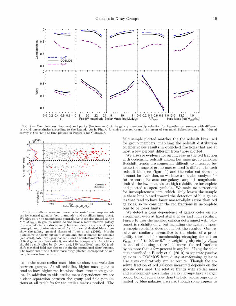
Galaxies in X-ray Groups 19

0.0 0.2 0.4 0.6 0.8 1.0z

0.4

0.6

0.8

1.0

Pu

rity

18 20 22 24F814W magnitude

9 10 11Stellar Mass [log(M

H/M

O •)]

0.0 0.2 0.4 0.6 0.8 1.0R/R200c

13.0 13.5 14.0Halo Mass [log(M200c/MO •

)]

0.4

0.6

0.8

1.0

Co

mp

lete

ne

ss

σX=3"

COSMOS

σX=1’

Fig. 8.— Completeness (top row) and purity (bottom row) of the galaxy membership selection for hypothetical surveys with differentcentroid uncertainties according to the legend. As in Figure 7, each curve represents the mean of ten mock lightcones, and the fiducialsurvey is the same as that plotted in Figure 5 for COSMOS.

-1

0

1

2

3

4

5

6

C ≡

M(N

UV

)-M

(R)

0 2 4 6∝ dN/dC

CentralsSatellites

10.5 11.0 11.5 12.0Stellar Mass [log(M

H/M

O •)]

0

10

20

∝ d

N/d

log

(M)

Fig. 9.— Stellar masses and unextincted rest-frame template col-ors for central galaxies (red diamonds) and satellites (gray dots).We plot only the unambigous centrals, i.e.those designated as theMMGGscale in groups which do not have a more massive galaxyin the outskirts or a discrepancy between identification with spec-troscopic and photometric redshifts. Horizontal dashed black linesshow the galaxy spectral classes of Ilbert et al. (2010). Marginplots show the distribution of colors and stellar masses for centrals(red solid), satellites (gray dashed), and a redshift-matched sampleof field galaxies (blue dotted), rescaled for comparison. Axis labelsshould be multiplied by 15 (centrals), 150 (satellites), and 500 (red-shift matched field sample) to obtain the normalized distributions.The lower end of the stellar mass range plotted corresponds to ourcompleteness limit at z = 1.

ies in the same stellar mass bins to show the variationbetween groups. At all redshifts, higher mass galaxiestend to have higher red fractions than lower mass galax-ies. In addition to this stellar mass dependence, we seea clear separation between the group and field popula-tions at all redshifts for the stellar masses probed. The

field sample plotted matches the the redshift bins usedfor group members; matching the redshift distributionon finer scales results in quenched fractions that are atmost a few percent different from those plotted.

We also see evidence for an increase in the red fractionwith decreasing redshift among low mass group galaxies.Redshift trends are somewhat difficult to interpret be-cause the range of group masses used is different in eachredshift bin (see Figure 1) and the color cut does notaccount for evolution, so we leave a detailed analysis forfuture work. Because our galaxy sample is magnitude-limited, the low mass bins at high redshift are incompleteand plotted as open symbols. We make no correctionsfor incompleteness here, which likely leaves the samplein these bins biased toward the detection of blue galax-ies that tend to have lower mass-to-light ratios than redgalaxies, so we consider the red fractions in incompletebins to be lower limits.

We detect a clear dependence of galaxy color on en-vironment, even at fixed stellar mass and high redshift.Figure 10 uses the member catalog determined with pho-tometric redshifts only, but including the available spec-troscopic redshifts does not affect the results. Our re-sults are similarly insensitive to the choice of a prob-ability threshold for membership; changing the cut onPmem > 0.5 to 0.3 or 0.7 or weighting objects by Pmem

instead of choosing a threshold moves the red fractionsby no more than a few percent in any bin. Using the colorcuts described in Bundy et al. (2010) to separate passivegalaxies in COSMOS from dusty star-forming galaxiesalso gives qualitatively similar results. Though the ab-solute fraction of red galaxies measured depends on thespecific cuts used, the relative trends with stellar massand environment are similar; galaxy groups have a largerproportion of red galaxies than the field, and groups dom-inated by blue galaxies are rare, though some appear to

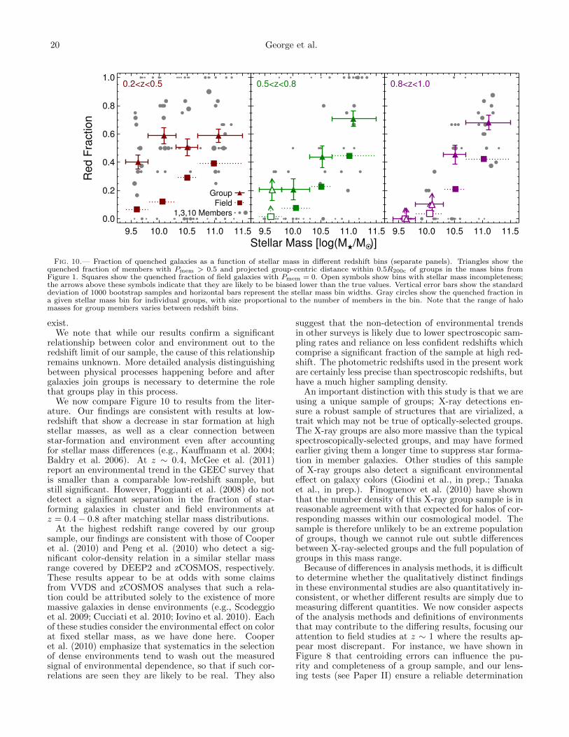
20 George et al.

Stellar Mass [log(MH/M

O •)]

Red F

raction

9.5 10.0 10.5 11.0 11.5

0.0

0.2

0.4

0.6

0.8

1.0

Group

Field

1,3,10 Members

0.2<z<0.5

9.5 10.0 10.5 11.0 11.5

0.5<z<0.8

9.5 10.0 10.5 11.0 11.5

0.8<z<1.0

Fig. 10.— Fraction of quenched galaxies as a function of stellar mass in different redshift bins (separate panels). Triangles show thequenched fraction of members with Pmem > 0.5 and projected group-centric distance within 0.5R200c of groups in the mass bins fromFigure 1. Squares show the quenched fraction of field galaxies with Pmem = 0. Open symbols show bins with stellar mass incompleteness;the arrows above these symbols indicate that they are likely to be biased lower than the true values. Vertical error bars show the standarddeviation of 1000 bootstrap samples and horizontal bars represent the stellar mass bin widths. Gray circles show the quenched fraction ina given stellar mass bin for individual groups, with size proportional to the number of members in the bin. Note that the range of halomasses for group members varies between redshift bins.

exist.We note that while our results confirm a significant

relationship between color and environment out to theredshift limit of our sample, the cause of this relationshipremains unknown. More detailed analysis distinguishingbetween physical processes happening before and aftergalaxies join groups is necessary to determine the rolethat groups play in this process.

We now compare Figure 10 to results from the liter-ature. Our findings are consistent with results at low-redshift that show a decrease in star formation at highstellar masses, as well as a clear connection betweenstar-formation and environment even after accountingfor stellar mass differences (e.g., Kauffmann et al. 2004;Baldry et al. 2006). At z ∼ 0.4, McGee et al. (2011)report an environmental trend in the GEEC survey thatis smaller than a comparable low-redshift sample, butstill significant. However, Poggianti et al. (2008) do notdetect a significant separation in the fraction of star-forming galaxies in cluster and field environments atz = 0.4− 0.8 after matching stellar mass distributions.

At the highest redshift range covered by our groupsample, our findings are consistent with those of Cooperet al. (2010) and Peng et al. (2010) who detect a sig-nificant color-density relation in a similar stellar massrange covered by DEEP2 and zCOSMOS, respectively.These results appear to be at odds with some claimsfrom VVDS and zCOSMOS analyses that such a rela-tion could be attributed solely to the existence of moremassive galaxies in dense environments (e.g., Scodeggioet al. 2009; Cucciati et al. 2010; Iovino et al. 2010). Eachof these studies consider the environmental effect on colorat fixed stellar mass, as we have done here. Cooperet al. (2010) emphasize that systematics in the selectionof dense environments tend to wash out the measuredsignal of environmental dependence, so that if such cor-relations are seen they are likely to be real. They also

suggest that the non-detection of environmental trendsin other surveys is likely due to lower spectroscopic sam-pling rates and reliance on less confident redshifts whichcomprise a significant fraction of the sample at high red-shift. The photometric redshifts used in the present workare certainly less precise than spectroscopic redshifts, buthave a much higher sampling density.

An important distinction with this study is that we areusing a unique sample of groups; X-ray detections en-sure a robust sample of structures that are virialized, atrait which may not be true of optically-selected groups.The X-ray groups are also more massive than the typicalspectroscopically-selected groups, and may have formedearlier giving them a longer time to suppress star forma-tion in member galaxies. Other studies of this sampleof X-ray groups also detect a significant environmentaleffect on galaxy colors (Giodini et al., in prep.; Tanakaet al., in prep.). Finoguenov et al. (2010) have shownthat the number density of this X-ray group sample is inreasonable agreement with that expected for halos of cor-responding masses within our cosmological model. Thesample is therefore unlikely to be an extreme populationof groups, though we cannot rule out subtle differencesbetween X-ray-selected groups and the full population ofgroups in this mass range.

Because of differences in analysis methods, it is difficultto determine whether the qualitatively distinct findingsin these environmental studies are also quantitatively in-consistent, or whether different results are simply due tomeasuring different quantities. We now consider aspectsof the analysis methods and definitions of environmentsthat may contribute to the differing results, focusing ourattention to field studies at z ∼ 1 where the results ap-pear most discrepant. For instance, we have shown inFigure 8 that centroiding errors can influence the pu-rity and completeness of a group sample, and our lens-ing tests (see Paper II) ensure a reliable determination

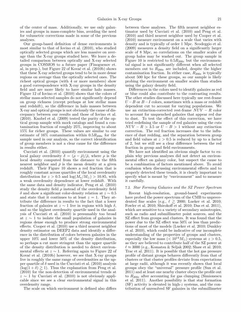
Galaxies in X-ray Groups 21

of the center of mass. Additionally, we use only galax-ies and groups in mass-complete bins, avoiding the needfor volumetric corrections made in some of the previousanalyses.

Our group-based definition of dense environments ismost similar to that of Iovino et al. (2010), who studiedoptically selected groups which are less massive on aver-age than the X-ray groups studied here. We leave a de-tailed comparison between optically and X-ray selectedgroups in COSMOS to a future paper (Finoguenov et.al, in prep.), but Figure 22 of Kovac et al. (2010b) showsthat these X-ray selected groups tend to be in more denseregions on average than the optically selected ones. Therichest optical groups (with 4 or more members) showa good correspondence with X-ray groups in the densityfield and are more likely to have similar halo masses.Figure 12 of Iovino et al. (2010) shows that the colors ofstellar mass-selected samples do not significantly dependon group richness (except perhaps at low stellar massand redshift), so the difference in halo masses betweenX-ray and optical groups is not obviously the cause of dis-crepancy between our results and those of Iovino et al.(2010). Knobel et al. (2009) tested the purity of the op-tical group sample with mock catalogs and found a con-tamination fraction of roughly 25%, improving to about15% for richer groups. These values are similar to ourestimate of 16% contamination within 0.5R200c for thesample used in our analysis, so the correct identificationof group members is not a clear cause for the differencein results either.

Cucciati et al. (2010) quantify environment using thelocal galaxy overdensity δ = (ρ − ρ)/ρ, where ρ is thelocal density computed from the distance to the fifthnearest neighbor and ρ is the mean density at a givenredshift. Their Figure 10 shows a red fraction that isroughly constant across quartiles of the local overdensitydistribution for z > 0.5 and log(M?/M) > 10.85, witha weak overdensity dependence at lower redshift. Withthe same data and density indicator, Peng et al. (2010)study the density field ρ instead of the overdensity fieldδ and show a significant color-density relation at z ∼ 0.5and state that it continues to at least z = 1. They at-tribute the difference in results to the fact that a lowerfraction of galaxies at z ∼ 1 live in regions with high δ,and so the highest overdensity quartile used in the anal-ysis of Cucciati et al. (2010) is presumably too broadat z ∼ 1 to isolate the small population of galaxies inregions dense enough to produce strong environmentaleffects. Cooper et al. (2010) use a third nearest neighbordensity estimator on DEEP2 data and identify a differ-ence in the distribution of colors between galaxies in theupper 10% and lower 50% of the density distribution,so perhaps a cut more stringent than the upper quartileof the density distribution is needed to detect environ-mental effects at z ∼ 1. Referring again to Figure 22 ofKovac et al. (2010b) however, we see that X-ray groupslive in roughly the same range of overdensities as the up-per quartile of δ used in the Cucciati et al. (2010) analysis(log(1 + δ) & 1). Thus the explanation from Peng et al.(2010) for the non-detection of environmental trends atz ∼ 1 by Cucciati et al. (2010) is not obviously appli-cable since we see a clear environmental signal in thisoverdensity range.

The scale on which environment is defined also differs

between these analyses. The fifth nearest neighbor es-timator used by Cucciati et al. (2010) and Peng et al.(2010) and third nearest neighbor used by Cooper et al.(2010) measure environment on a scale that varies withdensity and is typically of order 1 Mpc. Scodeggio et al.(2009) measures a density field on a significantly largerscale of 8 Mpc, so correlations on the smaller scales ofgroup halos may be washed out. The group sample inFigure 10 is restricted to 0.5R200c but the environmen-tal signal is not significantly different when all selectedmembers out to R200c are included, despite the highercontamination fraction. In either case, R200c is typicallyabout 500 kpc for these groups, so our sample is likelyprobing the environment on smaller scales than studiesusing the galaxy density field.

Differences in the colors used to identify galaxies as redor blue could also contribute to the contrasting results.The other studies discussed here typically use rest-frameU −B or B−I colors, sometimes with a mass or redshiftdependent cut to account for varying populations. Weuse an extinction-corrected rest-frame NUV − R colorto account for unquenched galaxies that appear red dueto dust. To test the effect of this correction, we havetried redefining the sample of red galaxies using the cutsNUV − R > 3.5 or U − B > 1 without any extinctioncorrection. The red fraction increases due to the influ-ence of dust redding, and the separation between groupand field values at z > 0.5 is reduced by up to a factorof 2, but we still see a clear difference between the redfraction in group and field environments.

We have not identified an obvious single factor to ex-plain why previous analyses did not detect an environ-mental effect on galaxy color, but suspect the cause tobe a combination of factors mentioned above. To avoidconfusion when discussing environmental effects and toproperly detected these trends, it is clearly important tospecify what is meant by “environment” and to measureit carefully.

7.2. Star Forming Galaxies and the SZ Power Spectrum

Recent high-resolution, ground-based experimentshave probed the power spectrum of the CMB to unprece-dented fine scales (e.g., ` & 2000; Lueker et al. 2010;Fowler et al. 2010; Shirokoff et al. 2010; Das et al. 2011),which are sensitive to a variety of secondary anisotropies,such as radio and submillimeter point sources, and theSZ effect from groups and clusters. It was found that thepower due to the SZ effect was 50% or less than predic-tions of most of the models (Lueker et al. 2010; Dunkleyet al. 2010), which could be indicative of our incompleteunderstanding of the properties of groups and clusters,especially the low mass (< 1014M) systems at z > 0.5,as they are believed to contribute half of the SZ power at` ≈ 3000 (e.g., Komatsu & Seljak 2002; Shaw et al. 2010;Trac et al. 2011). It is possible that the hot gas pressureprofile of distant groups behaves differently from that ofclusters or that cluster profiles deviate from expectationsat large radii, although it was recently shown that localgroups obey the “universal” pressure profile (Sun et al.2011) and at least one nearby cluster obeys the profile outto R200c after accounting for gas clumping (Simionescuet al. 2011). Another possibility is that star formation(SF) activity is elevated in high-z systems, and the con-tribution of unresolved SF galaxies in the submillimeter

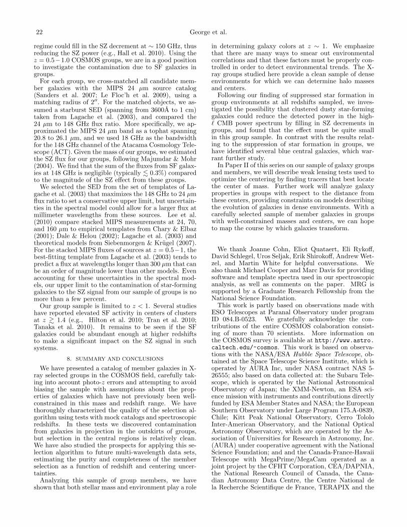
22 George et al.

regime could fill in the SZ decrement at ∼ 150 GHz, thusreducing the SZ power (e.g., Hall et al. 2010). Using thez = 0.5−1.0 COSMOS groups, we are in a good positionto investigate the contamination due to SF galaxies ingroups.

For each group, we cross-matched all candidate mem-ber galaxies with the MIPS 24 µm source catalog(Sanders et al. 2007; Le Floc’h et al. 2009), using amatching radius of 2′′. For the matched objects, we as-sumed a starburst SED (spanning from 3600A to 1 cm)taken from Lagache et al. (2003), and compared the24 µm to 148 GHz flux ratio. More specifically, we ap-proximated the MIPS 24 µm band as a tophat spanning20.8 to 26.1 µm, and we used 18 GHz as the bandwidthfor the 148 GHz channel of the Atacama Cosmology Tele-scope (ACT). Given the mass of our groups, we estimatedthe SZ flux for our groups, following Majumdar & Mohr(2004). We find that the sum of the fluxes from SF galax-ies at 148 GHz is negligible (typically . 0.3%) comparedto the magnitude of the SZ effect from these groups.

We selected the SED from the set of templates of La-gache et al. (2003) that maximizes the 148 GHz to 24 µmflux ratio to set a conservative upper limit, but uncertain-ties in the spectral model could allow for a larger flux atmillimeter wavelengths from these sources. Lee et al.(2010) compare stacked MIPS measurements at 24, 70,and 160 µm to empirical templates from Chary & Elbaz(2001); Dale & Helou (2002); Lagache et al. (2003) andtheoretical models from Siebenmorgen & Krugel (2007).For the stacked MIPS fluxes of sources at z = 0.5−1, thebest-fitting template from Lagache et al. (2003) tends topredict a flux at wavelengths longer than 300 µm that canbe an order of magnitude lower than other models. Evenaccounting for these uncertainties in the spectral mod-els, our upper limit to the contamination of star-forminggalaxies to the SZ signal from our sample of groups is nomore than a few percent.

Our group sample is limited to z < 1. Several studieshave reported elevated SF activity in centers of clustersat z & 1.4 (e.g., Hilton et al. 2010; Tran et al. 2010;Tanaka et al. 2010). It remains to be seen if the SFgalaxies could be abundant enough at higher redshiftsto make a significant impact on the SZ signal in suchsystems.

8. SUMMARY AND CONCLUSIONS

We have presented a catalog of member galaxies in X-ray selected groups in the COSMOS field, carefully tak-ing into account photo-z errors and attempting to avoidbiasing the sample with assumptions about the prop-erties of galaxies which have not previously been well-constrained in this mass and redshift range. We havethoroughly characterized the quality of the selection al-gorithm using tests with mock catalogs and spectroscopicredshifts. In these tests we discovered contaminationfrom galaxies in projection in the outskirts of groups,but selection in the central regions is relatively clean.We have also studied the prospects for applying this se-lection algorithm to future multi-wavelength data sets,estimating the purity and completeness of the memberselection as a function of redshift and centering uncer-tainties.

Analyzing this sample of group members, we haveshown that both stellar mass and environment play a role

in determining galaxy colors at z ∼ 1. We emphasizethat there are many ways to smear out environmentalcorrelations and that these factors must be properly con-trolled in order to detect environmental trends. The X-ray groups studied here provide a clean sample of denseenvironments for which we can determine halo massesand centers.

Following our finding of suppressed star formation ingroup environments at all redshifts sampled, we inves-tigated the possibility that clustered dusty star-forminggalaxies could reduce the detected power in the high-` CMB power spectrum by filling in SZ decrements ingroups, and found that the effect must be quite smallin this group sample. In contrast with the results relat-ing to the suppression of star formation in groups, wehave identified several blue central galaxies, which war-rant further study.

In Paper II of this series on our sample of galaxy groupsand members, we will describe weak lensing tests used tooptimize the centering by finding tracers that best locatethe center of mass. Further work will analyze galaxyproperties in groups with respect to the distance fromthese centers, providing constraints on models describingthe evolution of galaxies in dense environments. With acarefully selected sample of member galaxies in groupswith well-constrained masses and centers, we can hopeto map the course by which galaxies transform.

We thank Joanne Cohn, Eliot Quataert, Eli Rykoff,David Schlegel, Uros Seljak, Erik Shirokoff, Andrew Wet-zel, and Martin White for helpful conversations. Wealso thank Michael Cooper and Marc Davis for providingsoftware and template spectra used in our spectroscopicanalysis, as well as comments on the paper. MRG issupported by a Graduate Research Fellowship from theNational Science Foundation.

This work is partly based on observations made withESO Telescopes at Paranal Observatory under programID 084.B-0523. We gratefully acknowledge the con-tributions of the entire COSMOS colaboration consist-ing of more than 70 scientists. More information onthe COSMOS survey is available at http://www.astro.caltech.edu/~cosmos. This work is based on observa-tions with the NASA/ESA Hubble Space Telescope, ob-tained at the Space Telescope Science Institute, which isoperated by AURA Inc, under NASA contract NAS 5-26555; also based on data collected at: the Subaru Tele-scope, which is operated by the National AstronomicalObservatory of Japan; the XMM-Newton, an ESA sci-ence mission with instruments and contributions directlyfunded by ESA Member States and NASA; the EuropeanSouthern Observatory under Large Program 175.A-0839,Chile; Kitt Peak National Observatory, Cerro TololoInter-American Observatory, and the National OpticalAstronomy Observatory, which are operated by the As-sociation of Universities for Research in Astronomy, Inc.(AURA) under cooperative agreement with the NationalScience Foundation; and and the Canada-France-HawaiiTelescope with MegaPrime/MegaCam operated as ajoint project by the CFHT Corporation, CEA/DAPNIA,the National Research Council of Canada, the Cana-dian Astronomy Data Centre, the Centre National dela Recherche Scientifique de France, TERAPIX and the

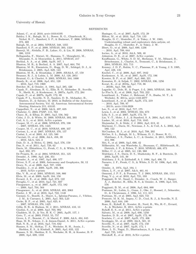
Galaxies in X-ray Groups 23

University of Hawaii.

REFERENCES

Adami, C., et al. 2010, arxiv:1010.6195Baldry, I. K., Balogh, M. L., Bower, R. G., Glazebrook, K.,

Nichol, R. C., Bamford, S. P., & Budavari, T. 2006, MNRAS,373, 469

Balogh, M., et al. 2004, MNRAS, 348, 1355Bamford, S. P., et al. 2009, MNRAS, 393, 1324Banerji, M., Abdalla, F. B., Lahav, O., & Lin, H. 2008, MNRAS,

386, 1219Bellagamba, F., Maturi, M., Hamana, T., Meneghetti, M.,

Miyazaki, S., & Moscardini, L. 2011, MNRAS, 217Berlind, A. A., et al. 2006, ApJS, 167, 1Blanton, M. R., & Berlind, A. A. 2007, ApJ, 664, 791Blanton, M. R., Eisenstein, D., Hogg, D. W., Schlegel, D. J., &

Brinkmann, J. 2005, ApJ, 629, 143Blanton, M. R., & Moustakas, J. 2009, ARA&A, 47, 159Brunner, R. J., & Lubin, L. M. 2000, AJ, 120, 2851Bruzual, G., & Charlot, S. 2003, MNRAS, 344, 1000Bundy, K., et al. 2006, ApJ, 651, 120—. 2010, ApJ, 719, 1969Butcher, H., & Oemler, A. 1984, ApJ, 285, 426Capak, P., Abraham, R. G., Ellis, R. S., Mobasher, B., Scoville,

N., Sheth, K., & Koekemoer, A. 2007a, ApJS, 172, 284Capak, P., et al. 2007b, ApJS, 172, 99Capak, P. L., Scoville, N. Z., Sanders, D. B., Mobasher, B.,

Masters, D., & Salvato, M. 2010, in Bulletin of the AmericanAstronomical Society, Vol. 42, American Astronomical SocietyMeeting Abstracts 215, 410.05

Cappelluti, N., et al. 2009, A&A, 497, 635Chabrier, G. 2003, PASP, 115, 763Chary, R., & Elbaz, D. 2001, ApJ, 556, 562Cohn, J. D., & White, M. 2009, MNRAS, 393, 393Coil, A. L., et al. 2010, ArXiv e-printsCooper, M. C., et al. 2006, MNRAS, 370, 198—. 2007, MNRAS, 376, 1445Cooper, M. C., et al. 2010, MNRAS, 409, 337Cortese, L., et al. 2007, MNRAS, 376, 157Csabai, I., et al. 2003, AJ, 125, 580Cucciati, O., et al. 2006, A&A, 458, 39—. 2010, A&A, 524, 2Dale, D. A., & Helou, G. 2002, ApJ, 576, 159Das, S., et al. 2011, ApJ, 729, 62Davis, M., Efstathiou, G., Frenk, C. S., & White, S. D. M. 1985,

ApJ, 292, 371De Propris, R., et al. 2004, MNRAS, 351, 125Dressler, A. 1980, ApJ, 236, 351Dressler, A., et al. 1997, ApJ, 490, 577Driver, S. P., et al. 2009, Astronomy and Geophysics, 50, 12Drory, N., et al. 2009, ApJ, 707, 1595Dunkley, J., et al. 2009, ApJS, 180, 306—. 2010, ArXiv e-printsEke, V. R., et al. 2004, MNRAS, 348, 866Elvis, M., et al. 2009, ApJS, 184, 158Evrard, A. E., et al. 2008, ApJ, 672, 122Feruglio, C., et al. 2010, ApJ, 721, 607Finoguenov, a., et al. 2007, ApJS, 172, 182—. 2009, ApJ, 704, 564Finoguenov, A., et al. 2010, MNRAS, 403, 2063Fowler, J. W., et al. 2010, ApJ, 722, 1148Gavazzi, G., Boselli, A., Mayer, L., Iglesias-Paramo, J., Vılchez,

J. M., & Carrasco, L. 2001, ApJ, 563, L23Gerke, B. F., et al. 2005, ApJ, 625, 6—. 2007, MNRAS, 376, 1425Gillis, B. R., & Hudson, M. J. 2011, MNRAS, 410, 13Giodini, S., et al. 2009, ApJ, 703, 982Gladders, M. D., & Yee, H. K. C. 2005, ApJS, 157, 1Goto, T., et al. 2003, PASJ, 55, 757Grove, L. F., Benoist, C., & Martel, F. 2009, A&A, 494, 845Haas, M. R., Schaye, J., & Jeeson-Daniel, A. 2011, ArXiv e-printsHall, N. R., et al. 2010, ApJ, 718, 632Hansen, S. M., McKay, T. A., Wechsler, R. H., Annis, J.,

Sheldon, E. S., & Kimball, A. 2005, ApJ, 633, 122Hansen, S. M., Sheldon, E. S., Wechsler, R. H., & Koester, B. P.

2009, ApJ, 699, 1333

Hasinger, G., et al. 2007, ApJS, 172, 29Hilton, M., et al. 2010, ApJ, 718, 133Hoaglin, D. C., Mosteller, F., & Tukey, J. W. 1983,

Understanding robust and exploratory data anlysis, ed.Hoaglin, D. C., Mosteller, F., & Tukey, J. W.

Ilbert, O., et al. 2009, ApJ, 690, 1236—. 2010, ApJ, 709, 644Iovino, A., et al. 2010, A&A, 509, 40Johnston, D. E., et al. 2007, ArXiv e-printsKauffmann, G., White, S. D. M., Heckman, T. M., Menard, B.,

Brinchmann, J., Charlot, S., Tremonti, C., & Brinkmann, J.2004, MNRAS, 353, 713

Kenney, J. D. P., Rubin, V. C., Planesas, P., & Young, J. S. 1995,ApJ, 438, 135

Knobel, C., et al. 2009, ApJ, 697, 1842Koekemoer, A. M., et al. 2007, ApJS, 172, 196Koester, B. P., et al. 2007, ApJ, 660, 221Komatsu, E., & Seljak, U. 2002, MNRAS, 336, 1256Kovac, K., et al. 2010a, ApJ, 718, 86—. 2010b, ApJ, 708, 505Lagache, G., Dole, H., & Puget, J.-L. 2003, MNRAS, 338, 555Le Floc’h, E., et al. 2009, ApJ, 703, 222Leauthaud, A., Tinker, J., Behroozi, P. S., Busha, M. T., &

Wechsler, R. 2011a, arxiv:1103.2077Leauthaud, A., et al. 2007, ApJS, 172, 219—. 2010, ApJ, 709, 97—. 2011b, arxiv:1104.0928Lee, N., et al. 2010, ApJ, 717, 175Lewis, I., et al. 2002, MNRAS, 334, 673Lilly, S. J., et al. 2007, ApJS, 172, 70Lin, Y.-T., Mohr, J. J., & Stanford, S. A. 2004, ApJ, 610, 745Lueker, M., et al. 2010, ApJ, 719, 1045Majumdar, S., & Mohr, J. J. 2004, ApJ, 613, 41Marinoni, C., Davis, M., Newman, J. A., & Coil, A. L. 2002, ApJ,

580, 122McCracken, H. J., et al. 2010, ApJ, 708, 202McGee, S. L., Balogh, M. L., Wilman, D. J., Bower, R. G.,

Mulchaey, J. S., Parker, L. C., & Oemler, A. 2011, MNRAS,413, 996

Mei, S., et al. 2009, ApJ, 690, 42Milkeraitis, M., van Waerbeke, L., Heymans, C., Hildebrandt, H.,

Dietrich, J. P., & Erben, T. 2010, MNRAS, 406, 673Miller, C. J., et al. 2005, AJ, 130, 968Mulchaey, J. S., Davis, D. S., Mushotzky, R. F., & Burstein, D.

2003, ApJS, 145, 39Mulchaey, J. S., & Zabludoff, A. I. 1998, ApJ, 496, 73Navarro, J. F., Frenk, C. S., & White, S. D. M. 1996, ApJ, 462,

563Oemler, A. 1974, ApJ, 194, 1Olsen, L. F., et al. 2007, A&A, 461, 81Osmond, J. P. F., & Ponman, T. J. 2004, MNRAS, 350, 1511Peng, Y.-j., et al. 2010, ApJ, 721, 193Poggianti, B. M., Smail, I., Dressler, A., Couch, W. J., Barger,

A. J., Butcher, H., Ellis, R. S., & Oemler, A. 1999, ApJ, 518,576

Poggianti, B. M., et al. 2008, ApJ, 684, 888Postman, M., Lubin, L., Gunn, J., Oke, J., Hoessel, J., Schneider,

D., & Christensen, J. 1996, AJ, 111, 615Postman, M., et al. 2005, ApJ, 623, 721Prescott, M. K. M., Impey, C. D., Cool, R. J., & Scoville, N. Z.

2006, ApJ, 644, 100Rozo, E., Rykoff, E., Koester, B., Nord, B., Wu, H.-Y., Evrard,

A., & Wechsler, R. 2011, ArXiv e-printsRykoff, E. S., et al. 2011, ArXiv e-printsSalvato, M., et al. 2009, ApJ, 690, 1250Sanders, D. B., et al. 2007, ApJS, 172, 86Scarlata, C., et al. 2007, ApJS, 172, 406Scodeggio, M., et al. 2009, A&A, 501, 21Scoville, N., et al. 2007, ApJS, 172, 150Scoville, N., et al. 2007, ApJS, 172, 1Shaw, L. D., Nagai, D., Bhattacharya, S., & Lau, E. T. 2010,

ApJ, 725, 1452Shirokoff, E., et al. 2010, ArXiv e-prints

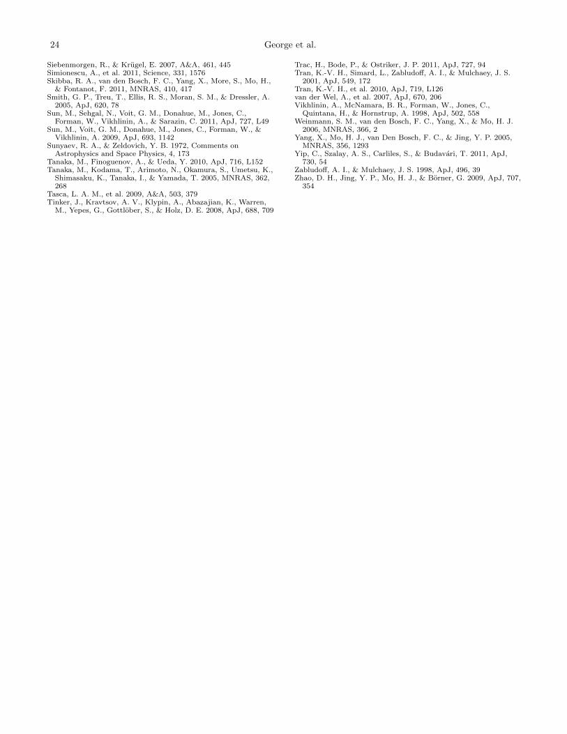
24 George et al.

Siebenmorgen, R., & Krugel, E. 2007, A&A, 461, 445Simionescu, A., et al. 2011, Science, 331, 1576Skibba, R. A., van den Bosch, F. C., Yang, X., More, S., Mo, H.,

& Fontanot, F. 2011, MNRAS, 410, 417Smith, G. P., Treu, T., Ellis, R. S., Moran, S. M., & Dressler, A.

2005, ApJ, 620, 78Sun, M., Sehgal, N., Voit, G. M., Donahue, M., Jones, C.,

Forman, W., Vikhlinin, A., & Sarazin, C. 2011, ApJ, 727, L49Sun, M., Voit, G. M., Donahue, M., Jones, C., Forman, W., &

Vikhlinin, A. 2009, ApJ, 693, 1142Sunyaev, R. A., & Zeldovich, Y. B. 1972, Comments on

Astrophysics and Space Physics, 4, 173Tanaka, M., Finoguenov, A., & Ueda, Y. 2010, ApJ, 716, L152Tanaka, M., Kodama, T., Arimoto, N., Okamura, S., Umetsu, K.,

Shimasaku, K., Tanaka, I., & Yamada, T. 2005, MNRAS, 362,268

Tasca, L. A. M., et al. 2009, A&A, 503, 379Tinker, J., Kravtsov, A. V., Klypin, A., Abazajian, K., Warren,

M., Yepes, G., Gottlober, S., & Holz, D. E. 2008, ApJ, 688, 709

Trac, H., Bode, P., & Ostriker, J. P. 2011, ApJ, 727, 94Tran, K.-V. H., Simard, L., Zabludoff, A. I., & Mulchaey, J. S.

2001, ApJ, 549, 172Tran, K.-V. H., et al. 2010, ApJ, 719, L126van der Wel, A., et al. 2007, ApJ, 670, 206Vikhlinin, A., McNamara, B. R., Forman, W., Jones, C.,

Quintana, H., & Hornstrup, A. 1998, ApJ, 502, 558Weinmann, S. M., van den Bosch, F. C., Yang, X., & Mo, H. J.

2006, MNRAS, 366, 2Yang, X., Mo, H. J., van Den Bosch, F. C., & Jing, Y. P. 2005,

MNRAS, 356, 1293Yip, C., Szalay, A. S., Carliles, S., & Budavari, T. 2011, ApJ,

730, 54Zabludoff, A. I., & Mulchaey, J. S. 1998, ApJ, 496, 39Zhao, D. H., Jing, Y. P., Mo, H. J., & Borner, G. 2009, ApJ, 707,

354