Embed Size (px)
Citation preview
A
Quasirandom Rumor Spreading
BENJAMIN DOERR, Max-Planck-Institut fur Informatik, GermanyTOBIAS FRIEDRICH, Friedrich-Schiller-Universitat Jena, GermanyTHOMAS SAUERWALD, University of Cambridge, U.K.
We propose and analyze a quasirandom analogue of the classical push model for disseminating information
in networks (“randomized rumor spreading”).In the classical model, in each round each informed vertex chooses a neighbor at random and informs
it, if it was not informed before. It is known that this simple protocol succeeds in spreading a rumor from
one vertex to all others within O(logn) rounds on complete graphs, hypercubes, random regular graphs,Erdos-Renyi random graph and Ramanujan graphs with probability 1 − o(1). In the quasirandom model,
we assume that each vertex has a (cyclic) list of its neighbors. Once informed, it starts at a random position
on the list, but from then on informs its neighbors in the order of the list. Surprisingly, irrespective of theorders of the lists, the above-mentioned bounds still hold. In some cases, even better bounds than for the
classical model can be shown.
Categories and Subject Descriptors: F.2.2 [Analysis of Algorithms and Problem Complexity]: Nonnu-merical Algorithms and Problems—Computations on discrete structures; G.2.2 [Discrete Mathematics]:Graph Theory—Graph algorithms
Additional Key Words and Phrases: Distributed computing, rumor spreading, broadcasting, quasi-randomness, random graphs, expander
1. INTRODUCTIONRandomized rumor spreading or random phone call protocols are simple randomizedepidemic algorithms designed to distribute a piece of information in a network. Theybuild on the basic paradigm that informed vertices call random neighbors to informthem (push model), or that uninformed vertices call random neighbors to become in-formed if the neighbor is (pull model). Despite the simple concept, these algorithmssucceed in distributing information extremely fast. In contrast to many natural deter-ministic approaches, they are also highly robust against transmission failures [Feigeet al. 1990; Karp et al. 2000; Elsasser and Sauerwald 2009].
This is the final draft (post refereeing) of a paper to appear in the ACM Transactions of Algorithms. Partof this work was done while Tobias Friedrich and Thomas Sauerwald were postdoctoral fellows at ICSIBerkeley supported by the German Academic Exchange Service (DAAD) or research associates at Max-Planck-Institut fur Informatik. Benjamin Doerr was partially supported by project DO 749/4 in the GermanResearch Foundation’s (DFG) Priority Program (SPP) 1307.Parts of the results appeared in the 19th ACM-SIAM Symposium on Discrete Algorithms (SODA ’08) [Doerret al. 2008] and the 36th International Colloquium on Automata, Languages and Programming(ICALP ’09) [Doerr et al. 2009].Authors’ addresses: B. Doerr, Max-Planck-Institut fur Informatik, Campus E1 4, 66123 Saarbrucken, Ger-many; T. Friedrich, Friedrich-Schiller-Universitat Jena, Ernst-Abbe-Platz 2, 07743 Jena, Germany, Email:[email protected]; T. Sauerwald, Computer Laboratory, William Gates Building, 15 JJ Thomson Av-enue, Cambridge CB3 0FD, United Kingdom, Email: [email protected];Permission to make digital or hard copies of part or all of this work for personal or classroom use is grantedwithout fee provided that copies are not made or distributed for profit or commercial advantage and thatcopies show this notice on the first page or initial screen of a display along with the full citation. Copyrightsfor components of this work owned by others than ACM must be honored. Abstracting with credit is per-mitted. To copy otherwise, to republish, to post on servers, to redistribute to lists, or to use any componentof this work in other works requires prior specific permission and/or a fee. Permissions may be requestedfrom Publications Dept., ACM, Inc., 2 Penn Plaza, Suite 701, New York, NY 10121-0701 USA, fax +1 (212)869-0481, or [email protected]© YYYY ACM 1549-6325/YYYY/01-ARTA $10.00
DOI 10.1145/0000000.0000000 http://doi.acm.org/10.1145/0000000.0000000
ACM Transactions on Algorithms, Vol. V, No. N, Article A, Publication date: January YYYY.
A:2 B. DOERR, T. FRIEDRICH, T. SAUERWALD
Such algorithms have been applied successfully both in the context where a singleitem of news has to be distributed from one processor to all others (cf. [Hedetniemiet al. 1988]), and in the case where news may be injected at various vertices at differ-ent times. The latter problem occurs when maintaining data integrity in distributeddatabases, e.g., name servers in large corporate networks [Demers et al. 1988; Kempeet al. 2003]. For a more extensive, but still concise discussion of various central aspectsof this area, we refer the reader to the paper by Karp et al. [2000].
1.1. Randomized Rumor SpreadingRumor spreading protocols often assume that all vertices have access to a central clock.The protocols then proceed in rounds, in each of which each vertex, independent of theothers, can perform certain actions. In the classical randomized rumor spreading pro-tocols, in each round each vertex contacts a neighbor chosen independently and uni-formly at random. In the push model, which we will focus on here, this results in thecontacted vertex becoming informed, provided it was not already. Since all communi-cations are done independently at random, in the following we shall call this also thefully random model to distinguish it from the quasirandom one we will propose in thispaper.
The first graphs for which the fully random model was analyzed are complete graphs[Frieze and Grimmett 1985; Pittel 1987]. Pittel [1987] proved that with probability1 − o(1), log2 n + lnn + f(n) rounds suffice, where f(n) can be any function tending toinfinity.
Feige et al. [1990] showed that on almost all random graphs G(n, p), p > (1 +ε) log n/n, the fully random model runs in O(log n) time with probability 1− n−1. Theyalso showed that this failure probability can be achieved for p = (log n+O(log log n))/nonly in Ω(log2 n) rounds. In addition, Feige et al. [1990] also considered hypercubesand proved a runtime bound of O(log n) with probability 1− n−1.
For expanders where the maximum and minimum degree satisfy ∆/δ = O(1), it wasshown in Sauerwald [2010] that the fully random model completes its broadcast cam-paign in O(log n) rounds with probability 1 − n−1 (similar results were shown earlier[Boyd et al. 2006; Mosk-Aoyama and Shah 2006], but these hold only for the push-pullmodel). Recently, Fountoulakis et al. [2010] and Fountoulakis and Panagiotou [2010]derived precise bounds on the runtime for random and pseudo-random regular graphs,extending the result of Frieze and Grimmett [1985] for complete graphs.
Demers et al. [1988] and Karp et al. [2000] introduced the push-pull model whichcombines push and pull transmissions. For this model, Chierichetti et al. [2010b;2010a] and Giakkoupis [2011] proved tight runtime bounds in terms of the conduc-tance. In particular, for any graph with constant conductance and arbitrary degreedistribution, a runtime bound of O(log n) was shown in [Giakkoupis 2011].
Rumor spreading has recently been studied intensively on social networks, modeledby random graphs that have a power law degree distribution. Chierichetti et al. [2011]showed that the push model with non-vanishing probability needs Ω(nα) rounds onpreferential attachment graphs [Barabasi and Albert 1999] for some α > 0. For suchpower-law networks, however, the push-pull strategy is much better than push or pullalone. With this strategy, O(log n) rounds suffice with high probability [Doerr et al.2011a]. Doerr et al. [2011a] further proved that for a slightly adjusted process, wherecontacts are chosen uniformly at random among all neighbors except the one that waschosen just in the round before,O(log n/ log log n) rounds suffice. This is asymptoticallyoptimal as the diameter of such a preferential attachment graphs, with power law ex-ponent 3, is Θ(log n/ log log n) [Bollobas et al. 2001]. Fountoulakis et al. [2012] showedthat push-pull requires Ω(log n) on Chung-Lu-random graphs [Chung and Lu 2002]
ACM Transactions on Algorithms, Vol. V, No. N, Article A, Publication date: January YYYY.
Quasirandom Rumor Spreading A:3
with power law exponent > 3 while for power law exponent ∈ (2, 3), the rumor spreadsto almost all nodes in time Θ(log log n) rounds with high probability.
1.2. Our ResultsIn this work, we propose a quasirandom analogue of the randomized rumor spreadingalgorithm. In this quasirandom model, every vertex is equipped with a cyclic list of itsneighbors. If a vertex becomes informed, then in the next round it chooses a position onthe list uniformly at random and informs the neighbor corresponding to this position.In the subsequent rounds, the vertex continues sending out messages in the order ofits list. Clearly, by introducing these dependencies we gain some natural advantageslike the fact that an informed vertex does not call a neighbor a second time beforehaving called all neighbors once. In consequence, we obtain an absolute guarantee thatafter ∆ diam(G) rounds all vertices are informed (see Theorem 3.1) improving over thecorresponding O(∆(diam(G) + log n)) bound of Feige et al. [1990] for the fully randommodel.
Surprisingly, we do not observe that the newly introduced dependencies are harmful.More precisely, we show that the O(log n) bound (valid with probability 1 − n−1) forcomplete graphs, hypercubes, random graphs, random regular graphs and Ramanujangraphs in the classical protocol also holds in the quasirandom model regardless ofwhich lists are used. In addition to its theoretical interest, this implies that in animplementation of the quasirandom protocol one may re-use any lists that are alreadypresent, e.g., to encode the network structure.
Our O(log n) runtime bound also applies to very sparse connected random graphswith p = (log n+ω(1))/n. This contrasts with a lower bound of Ω(log2 n) steps requiredby the fully random model to inform all vertices with probability 1 − n−1 [Feige et al.1990, Theorem 4.1] and with a lower bound on the expected time of Ω(log n log log n)shown in this paper. Similarly for hypercubes, we show that the quasirandom modelcompletes in O(log n) rounds with probability 1 − n−Ω(logn), while the fully randommodel is easily seen to require Ω(log2 n) steps to achieve the same probability of suc-cess. The interesting aspect of these improvements is not so much their actual mag-nitude, but rather that they can be achieved for free by using a very natural protocol.Note that also speed-ups not visible by asymptotic analyses have been observed, seethe experimental analysis [Doerr et al. 2011b]. For example, the quasirandom protocolwas seen to be around 10% faster on the hypercube on 4096 vertices and around 15%faster on random 12-regular graphs on 4096 vertices.
To prove the results in this paper, we need to cope with the more dependent randomexperiments. Recall that once a vertex has sent out a message, all its future trans-missions are determined. The methods we develop to cope with these difficulties, e.g.,suitably delaying independent random decisions to have enough independent random-ness at certain moments to allow the use of Chernoff-type inequalities, might be usefulin the analysis of other dependent settings as well.
Our analysis employs a certain graph class called expanding graphs, which is de-fined by three natural expansion properties. Roughly speaking, these properties re-quire that small sets of vertices have many neighbors, and for large sets of vertices theexternal vertices have many neighbors in the set, and finally that the vertex degreesare of similar order (see Definition 4.1 for the details). This graph class has been usedby other authors, e.g., in [Cooper et al. 2012]. We prove that complete graphs, ran-dom graphs, random regular graphs and Ramanujan graphs are expanding. After thatwe show that the quasirandom model succeeds in O(log n) rounds on every expandinggraph with probability 1− n−γ , where γ > 0 is an arbitrary constant.
ACM Transactions on Algorithms, Vol. V, No. N, Article A, Publication date: January YYYY.
A:4 B. DOERR, T. FRIEDRICH, T. SAUERWALD
1.3. Related Work on QuasirandomnessWe call an algorithm quasirandom if it imitates (or achieves in an even better way) aparticular property of a randomized algorithm deterministically. The concept of quasi-randomness occurs in several areas of mathematics and computer science. A promi-nent example are low-discrepancy point sets and Quasi-Monte Carlo Methods [Nieder-reiter 1992], which imitate the property of a random point set to be evenly distributedin their domain.
Our quasirandom rumor spreading protocol imitates two properties of the fully ran-dom counterpart, namely that a vertex over a short period of time does not contactneighbors twice and over a long period of time calls all neighbors roughly equally of-ten.
This is very much related to a quasirandom analogue of the classic random walk,which is also known as Eulerian walker [Priezzhev et al. 1996], edge ant walk [Wagneret al. 1999], whirling tour [Dumitriu et al. 2003], Propp machine [Kleber 2005; Cooperand Spencer 2006] and deterministic random walks [Cooper et al. 2007b; Doerr andFriedrich 2009]. Unlike in a random walk, in a quasirandom walk each vertex servesits neighbors in a fixed order. The resulting (completely deterministic) walk neverthe-less closely resembles a random walk in several respects [Cooper and Spencer 2006;Doerr and Friedrich 2009; Cooper et al. 2007b; Cooper et al. 2010; Friedrich and Sauer-wald 2010]. Other algorithmic applications of the idea of quasirandom walks are au-tonomous agents patrolling a territory [Wagner et al. 1996], external mergesort [Barveet al. 1997], and iterative load-balancing [Friedrich et al. 2010].
1.4. Results Obtained After This WorkSubsequent to the conference versions [Doerr et al. 2008; 2009] and during the prepa-ration of this journal version, the following results appeared that answer some ques-tions left open in this work. In [Angelopoulos et al. 2009], it is proven that with proba-bility 1− o(1), the quasirandom model succeeds in informing all vertices of a completegraph on n vertices in (1 + o(1))(log2 n + lnn) rounds. Hence for the complete graph,the quasirandom model achieves the same runtime as the fully random one [Friezeand Grimmett 1985] up to lower order terms. This was strengthened by Fountoulakisand Huber [2009], who nearly showed that also Pittel’s bounds [Pittel 1987] hold forthe quasirandom model—their upper and lower bounds deviate by only a Θ(log log n)term.
A second important aspect of broadcasting protocols is their robustness. The fullyrandom model, due to its high use of independent randomness is usually considered tobe very robust. See [Karp et al. 2000; Elsasser and Sauerwald 2009] for some resultsin this direction. A very precise result, valid for both the fully random and the quasi-random model, was recently given in [Doerr et al. 2013]. They consider the setting thateach message reaches its destination only with an (independently sampled) probabilityof 0 < p < 1. Again for the complete graph on n vertices, they show that both protocolssucceed in (1 +o(1)) (log1+p n+p−1 lnn) rounds with probability 1−o(1). Together witha corresponding lower bound for the fully random model, this shows that both modelsare equally robust against transmission failures, in spite of the greatly reduced use ofindependent randomness in the quasirandom model.
The question of how much randomness is needed in such protocols was first consid-ered by Doerr and Fouz [2011] and Giakkoupis and Woelfel [2011]. Among other re-sults, the latter work presents a variant of the quasirandom model which requires onaverage only O(log log n) instead of O(log n) random bits per vertex in order to spreadthe rumor in O(log n) rounds on a complete graph with probability 1 − n−Ω(1). Gi-akkoupis et al. [2012] present two protocols that are based on hashing and pseudoran-
ACM Transactions on Algorithms, Vol. V, No. N, Article A, Publication date: January YYYY.
Quasirandom Rumor Spreading A:5
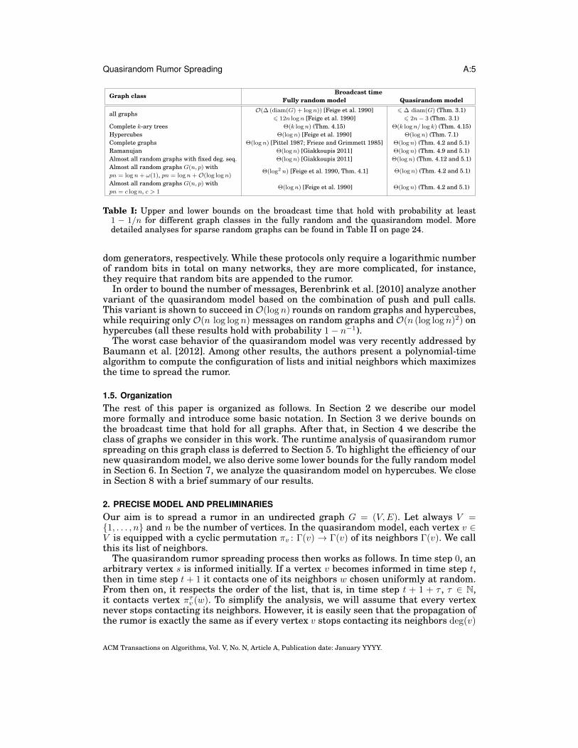
Graph class Broadcast timeFully random model Quasirandom model
all graphs O(∆ (diam(G) + logn)) [Feige et al. 1990] 6 ∆ diam(G) (Thm. 3.1)6 12n logn [Feige et al. 1990] 6 2n− 3 (Thm. 3.1)
Complete k-ary trees Θ(k logn) (Thm. 4.15) Θ(k logn/ log k) (Thm. 4.15)Hypercubes Θ(logn) [Feige et al. 1990] Θ(logn) (Thm. 7.1)Complete graphs Θ(logn) [Pittel 1987; Frieze and Grimmett 1985] Θ(logn) (Thm. 4.2 and 5.1)Ramanujan Θ(logn) [Giakkoupis 2011] Θ(logn) (Thm. 4.9 and 5.1)Almost all random graphs with fixed deg. seq. Θ(logn) [Giakkoupis 2011] Θ(logn) (Thm. 4.12 and 5.1)Almost all random graphs G(n, p) with
Θ(log2 n) [Feige et al. 1990, Thm. 4.1] Θ(logn) (Thm. 4.2 and 5.1)pn = logn+ ω(1), pn = logn+O(log logn)
Almost all random graphs G(n, p) withΘ(logn) [Feige et al. 1990] Θ(logn) (Thm. 4.2 and 5.1)
pn = c logn, c > 1
Table I: Upper and lower bounds on the broadcast time that hold with probability at least1 − 1/n for different graph classes in the fully random and the quasirandom model. Moredetailed analyses for sparse random graphs can be found in Table II on page 24.
dom generators, respectively. While these protocols only require a logarithmic numberof random bits in total on many networks, they are more complicated, for instance,they require that random bits are appended to the rumor.
In order to bound the number of messages, Berenbrink et al. [2010] analyze anothervariant of the quasirandom model based on the combination of push and pull calls.This variant is shown to succeed inO(log n) rounds on random graphs and hypercubes,while requiring only O(n log log n) messages on random graphs and O(n (log log n)2) onhypercubes (all these results hold with probability 1− n−1).
The worst case behavior of the quasirandom model was very recently addressed byBaumann et al. [2012]. Among other results, the authors present a polynomial-timealgorithm to compute the configuration of lists and initial neighbors which maximizesthe time to spread the rumor.
1.5. OrganizationThe rest of this paper is organized as follows. In Section 2 we describe our modelmore formally and introduce some basic notation. In Section 3 we derive bounds onthe broadcast time that hold for all graphs. After that, in Section 4 we describe theclass of graphs we consider in this work. The runtime analysis of quasirandom rumorspreading on this graph class is deferred to Section 5. To highlight the efficiency of ournew quasirandom model, we also derive some lower bounds for the fully random modelin Section 6. In Section 7, we analyze the quasirandom model on hypercubes. We closein Section 8 with a brief summary of our results.
2. PRECISE MODEL AND PRELIMINARIESOur aim is to spread a rumor in an undirected graph G = (V,E). Let always V =1, . . . , n and n be the number of vertices. In the quasirandom model, each vertex v ∈V is equipped with a cyclic permutation πv : Γ(v) → Γ(v) of its neighbors Γ(v). We callthis its list of neighbors.
The quasirandom rumor spreading process then works as follows. In time step 0, anarbitrary vertex s is informed initially. If a vertex v becomes informed in time step t,then in time step t + 1 it contacts one of its neighbors w chosen uniformly at random.From then on, it respects the order of the list, that is, in time step t + 1 + τ , τ ∈ N,it contacts vertex πτv (w). To simplify the analysis, we will assume that every vertexnever stops contacting its neighbors. However, it is easily seen that the propagation ofthe rumor is exactly the same as if every vertex v stops contacting its neighbors deg(v)
ACM Transactions on Algorithms, Vol. V, No. N, Article A, Publication date: January YYYY.
A:6 B. DOERR, T. FRIEDRICH, T. SAUERWALD
rounds after it got informed. We denote by It the set of vertices that are informed atthe end of time step t.
Note that the assumption that the initial vertex contacted first by an informed vertexis chosen uniformly at random is crucial for the quasirandom protocol. If the adversarywas allowed to specify the initial vertices also, then the time to inform all vertices couldtake up to n− 1 steps, for example, on a complete graph.
In the remainder of this paper, it will be convenient to consider a model equivalentto the quasirandom model. This model uses the so-called ever-rolling lists assumption,where we assume that vertices contact neighbors at all times, informing the neighbors(if the vertex is informed herself). Hence, here each vertex v, already at the start of theprotocol, chooses a neighbor iv uniformly at random from Γ(v). This is the neighbor itcontacts at time t = 1. In each following time step t = 2, 3, . . ., the vertex v contacts thevertex πt−1
v (iv) and informs it, if it was not yet informed and if v is informed at thattime (here, πt−1
v is the (t− 1)-th composition of π with itself).From the viewpoint of how the information spreads, the model with the ever-rolling
lists assumption yields a process equivalent to the standard quasirandom rumorspreading model. Hence in the remainder of the paper, we shall always be discussingthe model with ever-rolling lists unless we say otherwise.
We shall analyze how long it takes until a rumor known to a single vertex is spreadto all other vertices. We adopt a worst-case view in that we aim at bounds that areindependent of the starting vertex and of all lists present in the model. This suggeststhe following definitions.
Definition 2.1. Let G = (V,E) be a graph and s ∈ V . Then by Rs we denote the ran-dom variable describing the first time t at which the random rumor spreading processstarted in the vertex s leads to all vertices being informed. Let R(G) be the (unique)minimal integer-valued random variable that dominates all Rs, i.e., for every s ∈ Vand t ∈ N it holds that
Pr [R(G) > t] > Pr [Rs > t] .
We call R(G) the broadcast time of the randomized rumor spreading protocol on thegraph G1.
Let L = (πv)v∈V be a family of lists. By QL,s we denote the (random) first time thatthe quasirandom rumor spreading protocol with lists L started in s succeeds in inform-ing all vertices. LetQ(G) be the (unique) minimal integer valued random variable thatdominates all QL,s, i.e., for every family of lists L, every s ∈ V and t ∈ N it holds that
Pr [Q(G) > t] > Pr [QL,s > t] .
We call Q(G) the broadcast time of the quasirandom rumor spreading protocol on thegraph G.
In the analysis it will often be convenient to assume that after receiving the rumor,a vertex does not pass it on for a certain number of time steps (delaying). Also, it willbe helpful to ignore all messages that certain vertices send out from a certain timeonward (ignoring). Since we assumed all random decisions done by the vertices beforethe start of the protocol (ever-rolling list assumption), an easy induction shows thatany delaying and ignoring assumptions (possibly even relying on the random choicesdone by the vertices which have not been active yet) for each vertex can only increase
1In order to see that R(G) is well-defined, note that for every t there exists one vertex s = s(t) suchthat Pr [Rs(G) > t] is maximized. Then we let R(G) satisfy Pr [R(G) > t] = Pr [Rs(G) > t]. Doing thisfor all integers t ∈ N yields a sequence Pr [R(G) > t] : t ∈ N of non-increasing values in [0, 1]. Hence,Pr [R(G) = t] := Pr [R(G) > t]−Pr [R(G) > t+ 1] completes the definition of R(G).
ACM Transactions on Algorithms, Vol. V, No. N, Article A, Publication date: January YYYY.
Quasirandom Rumor Spreading A:7
the round in which it becomes informed. In consequence, these assumptions can onlyincrease the time needed to inform all vertices. More precisely, the random variabledescribing the broadcast time of any model with delaying and ignoring assumptionsdominates the original one (see Definition A.1 for the precise definition of stochasticdomination).
LEMMA 2.1. For all possible delaying and ignoring assumptions, the random vari-able describing the broadcast time of the quasirandom model with these assumptionsis stochastically larger than the broadcast time of the true quasirandom model.
We use both delaying and ignoring to reduce the number of dependencies in theanalysis. We do this by splitting the analysis into phases. All vertices that receive therumor within this phase (newly informed vertices) are assumed to delay their actionsuntil the beginning of the next phase. From this next phase on, all messages fromvertices that previously sent out messages are ignored. Thus, we start each phase withonly newly informed vertices acting. Since they have not actively participated in therumor spreading process, the first neighbors to which they send the rumor are chosenindependently.
We will also need chains of contacting vertices. That is, we say a vertex u1 ∈ Vreaches another vertex um ∈ V within the time interval [a, b], if there is a path(u1, u2, . . . , um) in G and t1 < t2 < · · · < tm−1 ∈ [a, b] such that for all j ∈ [1,m − 1],πtj−1uj (iuj ) = uj+1. For a vertex w ∈ V , we denote by U[a,b](w) the set of vertices that
reach w within the time interval [a, b].
Other NotationThroughout the paper, we use the following graph-theoretical notation. For a vertex vof a graph G = (V,E), let Γ(v) := u ∈ V : u, v ∈ E be the set of its neighbors anddeg(v) := |Γ(v)| its degree. For any S ⊆ V , let degS(v) := |Γ(v) ∩ S|. For any S1, S2 ⊆ V ,let E(S1, S2) := (u, v) ∈ E : u ∈ S1 ∧ v ∈ S2. Let δ := minv∈V deg(v) be the minimumdegree, d := 2|E|/n the average degree, and ∆ := maxv∈V deg(v) the maximum degree.The distance dist(x, y) between vertices x and y is the length of a shortest path fromx to y. The diameter diam(G) of a connected graph G is the largest distance betweentwo vertices in G. We will also use Γk(u) := v ∈ V : dist(u, v) = k and Γ6k(u) := v ∈V : dist(u, v) 6 k. For sets S we define Γ(S) := v ∈ V : ∃u ∈ S, u, v ∈ E as the setof neighbors of S. The complement of a set S is denoted Sc := V \ S.
All logarithms log n are natural logarithms to the base e. As we are only interestedin the asymptotic behavior, we will sometimes assume that n is sufficiently large.
3. QUASIRANDOM RUMOR SPREADING ON GENERAL GRAPHSIn this section, we prove two bounds for the broadcast time valid for all graphs. Thecorresponding upper bounds for the fully random model are O(∆ (diam(G)+log n)) and12n log n, both satisfied with probability 1− 1/n [Feige et al. 1990].
THEOREM 3.1. For any graph G = (V,E), the broadcast time of the quasirandommodel is at most
(1) ∆ · diam(G) with probability 1, and(2) 2n− 3 with probability 1.
Proof. Let u be the vertex initially informed.Let v ∈ V and P = (u = u0, u1, . . . , u` = v) be a shortest path from u to v. Clearly
for all i 6 `, ui becomes informed at most deg(ui−1) 6 ∆ time-steps after ui−1 becameinformed. Claim (i) follows.
ACM Transactions on Algorithms, Vol. V, No. N, Article A, Publication date: January YYYY.
A:8 B. DOERR, T. FRIEDRICH, T. SAUERWALD
To prove claim (ii), again let v ∈ V and let P = (u = u0, u1, . . . , u` = v) be a short-est path from u to v. Let w be a vertex not lying on P . Then, as observed alreadyin [Feige et al. 1990], w has at most three neighbors on P , and these are contained inui−1, ui, ui+1 for some i < `. If w has exactly three neighbors ui−1, ui, ui+1 on P , wecall it a counterfeit of ui (as ui and w have, apart from each other, the same neigh-bors on P ). Denote by C(ui) the set of counterfeits of ui. Without loss of generality, wemay choose P in such a way that for all i < `, ui is informed no later than any if itscounterfeits.
Note also that any vertex ui on the path has only ui−1 and ui+1 (if existent) as neigh-bors on the path.
Let ti denote the time that vertex ui becomes informed. Then, t0 = 0. By definitionof our algorithm and choice of P , we have t1 6 t0 + |Γ(u0) \ C(u1)| = t0 + |Γ(u0) \P | + 1 − |C(u1)|. For 2 6 i 6 ` − 1, similarly, we have ti 6 ti−1 + |Γ(ui−1) \ C(ui)| =ti−1 + |Γ(ui−1) \ P |+ 2− |C(ui)|. Finally, t` 6 t`−1 + |Γ(u`−1) \ P |+ 2. We conclude
t` 6`−1∑i=0
|ΓV (ui) \ P | −`−1∑i=1
|C(ui)|+ 2`− 1.
Now each vertex w not lying on P can contribute at most 2 to the above expression (if ithas three neighbors on P , then it is also a counterfeit). Hence t` 6 2(n−`−1)+2`−1 =2n− 3.
It is easy to verify that for a path of length n − 1 there are lists and initial verticessuch that 2n − 3 rounds are needed. Hence the second bound is tight. The first boundis matched by k-ary trees (up to constant factors), as shown in Section 4.3, where wealso demonstrate that the quasirandom model is faster than the fully random one onthese graphs.
4. GRAPH CLASSESOur results cover hypercubes, many expander graphs, random regular graphs, andErdos-Renyi random graphs. The three latter graph classes have three properties incommon, to which we will refer as “expanding”. This allows us to examine the quasi-random rumor spreading on them from a higher level just using these three propertiesdefined in the following Section 4.1.
4.1. Expanding GraphsIn order to analyze our quasirandom rumor spreading model for a larger class ofgraphs at once, we distill three simple properties of graphs which are satisfied byseveral common graph classes. Given these three properties, we can later prove inTheorem 5.1 that quasirandom rumor spreading successfully informs all vertices in alogarithmic runtime. Roughly speaking, these properties concern the vertex expansionof not too large subsets (P1), the edge expansion (P2) and the regularity of the graph(P3).
Definition 4.1 (expanding graphs). We call a connected graph expanding if the fol-lowing properties hold:
(P1). For any constant Cα with 0 < Cα 6 d/2 there is a constant Cβ ∈ (0, 1)such that for any connected subset S ⊆ V with 3 6 |S| 6 Cα (n/d), it holds that|Γ(S) \ S| > Cβ d |S|.(P2). There are constants Cδ ∈ (0, 1) and Cω > 0 such that for any subset S ⊆ V ,the number of vertices in Sc which have at least Cδd(|S|/n) neighbors in S is atleast |Sc| − Cωn
2
d|S| .
ACM Transactions on Algorithms, Vol. V, No. N, Article A, Publication date: January YYYY.
Quasirandom Rumor Spreading A:9
(P3). d = Ω(∆) and if d = ω(log n), then also d = O(δ).
We will now describe the properties in detail and argue why each of them is intrinsicfor the analysis. (P1) describes a vertex expansion, which means that connected setshave a neighborhood which is roughly in the order of the average degree larger thanthe set itself. Without this property, the broadcasting process could end up in a set witha tiny neighborhood and thereby slow down too much. Note that in (P1), Cβ dependson Cα. As Cα has to be a constant, the upper limit on Cα only applies for constant d.
(P2) is a certain edge expansion property implying that a large portion of unin-formed vertices has a sufficiently large number of informed neighbors. This avoids thesituation where the broadcasting process stumbles upon a point when it has informedmany vertices but most of the remaining uninformed vertices have very few informedneighbors and therefore only a small chance to get informed. Note that (P2) is onlyuseful for |S| = ω(n/d).
The last property (P3) demands a certain regularity of the graph. It is trivially ful-filled for regular graphs, which many definitions of expanders require. The conditiond = Ω(∆) for the case d = O(log n) does not limit any of our graph classes below. If theaverage degree is at most logarithmic, (P3) implies no further restrictions. Otherwise,we require δ, d and ∆ to be of the same order of magnitude. Without this condition,there could be an uninformed vertex with δ informed neighbors of degree ω(δ) whichdoes not get informed in logarithmic time with a good probability. With an additionalfactor of ∆/δ this could be resolved, but as we aim at a logarithmic bound, we requireδ = Θ(∆) for d = ω(log n). Note that we do not require d = ω(1), but the proof tech-niques for constant and non-constant average degrees will differ in Section 5.
We now describe several important graph classes which are expanding, i.e., satisfyall three properties of Definition 4.1, with high probability.
4.1.1. Complete Graph. It is not difficult to show that complete graphs are expanding.
THEOREM 4.1. Complete graphs are expanding.
Proof. We first prove that (P1) holds. Let Cα be an arbitrary constant. Take any subsetS ⊆ V with 3 6 |S| 6 Cαn/(n− 1). Then
|Γ(S) \ S| = n− |S| > |S| (n− 1)n− |S||S|n
= |S| (n− 1)
(1
|S|− 1
n
),
so (P1) holds with Cβ = 1|S| −
1n > n−1
Cαn− 1
n > 0. We now show that (P2) holds. LetCδ ∈ (0, 1) be an arbitrary constant. Take any subset S ⊆ V . Then every vertex v ∈ Schas exactly |S| > Cδd(|S|/n) neighbors in S which implies that (P2) is satisfied.
Property (P3) is trivially fulfilled, as a complete graph is regular.
4.1.2. Random Graphs G(n, p), p > (logn + ω(1))/n. In this section we show that a largeclass of random graphs is expanding with probability 1− o(1). We use the popularrandom graph model G(n, p), where between each two vertices out of a set of n verticesan edge is present independently with probability p. This model is usually called theErdos-Renyi random graph model.
We distinguish two kinds of random graphs with slightly different properties:
Definition 4.2 (sparse and dense random graph). We call a random graph G(n, p)sparse if p = (log n + fn)/n with fn = ω(1) and fn = O(log n), and dense if p =ω(log(n)/n).
ACM Transactions on Algorithms, Vol. V, No. N, Article A, Publication date: January YYYY.
A:10 B. DOERR, T. FRIEDRICH, T. SAUERWALD
Note that our definition of a sparse random graph coincides with the one of Cooper andFrieze [2007] who set p = cn log(n)/n with (cn − 1) log n = ω(1) and cn = O(1). In theremainder of this section we prove the following theorem.
THEOREM 4.2. Sparse and dense random graphs are expanding with probability1− o(1).
The proof can be skipped at a first reading of the paper, since the following sectionsdo not depend on the proven results of this section.
Proof. Note that for random graphs, d = p (n − 1) (1 ± o(1)) holds with probability1− n−1. To simplify the presentation of the proof we will ignore the factor (1± o(1)) aswe do not try to optimize the used constants.
The easiest property to check is (P3). That d = Ω(∆) holds with probability 1− o(1)is a well-known property of random graphs and can be shown by union and Chernoffbounds (cf. Lemma A.1) as follows:
Pr [∆ > 5d] = Pr [∃v ∈ V : deg(v) > 5d] 6 n exp(−4d/3) = o(1).
Analogously for d = ω(log n),
Pr [δ 6 d/2] = Pr [∃v ∈ V : deg(v) 6 d/2] 6 n exp(−d/8) = o(1).
For the proof of (P2) it suffices to bound the number of neighbors of a set by Chernoffbounds. The following lemma does this for sparse and dense random graphs at once.
LEMMA 4.3. Sparse and dense random graphs satisfy (P2) with probability1− o(1).
Proof. We choose Cδ = 1/2 and Cω = 32. Consider a set S ⊆ V of arbitrary size |S| =s. We want to show that the number of vertices in Sc which have at least Cδds/nneighbors in S is at least |Sc| − Cω n
2
ds .Fix a vertex v ∈ Sc. Linearity of expectations implies E [degS(v)] =
∑u∈S p = ps.
Hence a Chernoff bound (Lemma A.1) gives
Pr [degS(v) 6 (1/2)E [degS(v)]] 6 exp
(− ds
8n
).
Hence the probability for the existence of a subset of vertices in Sc of size Cωn2/(ds)
being bad, i.e., the set has more than Cωn2
ds vertices with less than Cδds/n neighbors inS, can be bounded by(
n− sCωn2
ds
)exp
(− ds
8n
)Cωn2/(ds)
6 2n exp(−4n).
Taking the union bound over all possible sets S, we obtain
Pr [∃bad S] 6 2n · 2n exp(−4n) 6
(4
e4
)n.
We now turn to (P1). We first prove that (P1) holds for dense random graphs. Af-ter that we extend it to sparse random graphs, which requires slightly more involvedarguments.
LEMMA 4.4. Dense random graphs satisfy (P1) with probability 1− o(1).
Proof. Let Cα > 0 be an arbitrary constant. Fix a set S ⊆ V of size s = |S| with1 6 s 6 Cα(n/d). We show that |Γ(S) \ S| > Cβds with Cβ := 1/(4(Cα + 1)).
ACM Transactions on Algorithms, Vol. V, No. N, Article A, Publication date: January YYYY.
Quasirandom Rumor Spreading A:11
The probability that a vertex v ∈ Sc is connected to a vertex in S is
1− (1− p)s > 1− exp(−ps).Linearity of expectation and using the fact that e−x 6 1
x+1 for any number x > 0 gives
E [|Γ(S) \ S|] > (n− s)(1− 1
ps+1
)=(n− o
(n
logn
))psps+1 > n
2ps
Cα+1 = 2Cβds.
Applying Chernoff bounds (Lemma A.1), we obtain
Pr [|Γ(S) \ S| 6 Cβ ds] 6 exp (−Cβds/4) .
It remains to show that this holds for all sets S. First, taking a union bound over allsets of size s, we obtain
Pr [∃S ⊆ V : |S| = s, |Γ(S) \ S| 6 Cβ ds] 6 ns exp (−Cβds/4) 6 n−ω(1),
where the last inequality uses the assumption d = ω(log n). Finally, a union bound overall possible values of s yields
Pr [∃S ⊆ V : |Γ(S) \ S| 6 Cβ ds] 6∑ns=1 n
−ω(1) = n−ω(1).
We now consider sparse random graphs. For this, we need the following three technicallemmas. The first one proves a slightly stronger bound compared to the original lemmain [Cooper and Frieze 2007, Property P2].
LEMMA 4.5. Sparse random graphs satisfy with probability 1− o(1) that for everysubset S ⊆ V of size s = O(n/d) it holds that |E(S, S)| = o(s log n).
Proof. We assume without loss of generality S 6= ∅. We bound the probability for theexistence of a set S of size s with |E(S, S)| > s logn√
log lognas follows:
Pr
[∃S : |E(S, S)| > s
log n√log log n
]6
(n
s
)( (s2
)s logn√
log logn
)ps logn√
log logn
6 ns
(s2 e
s logn√log logn
)s logn√log logn
ps logn√
log logn = ns(s e p√
log log n
log n
)s logn√log logn
= exp
(−s(
log n√log log n
log
(log n
s e p√
log log n
)− log n
))6 exp
(−Ω(log n
√log log n )− log n
)= n−ω(1),
where in the third inequality we used that s = O(n/d) and p = Θ(d/n) together implythat s e p = O(1). Taking the union bound over all values of s completes the proof.
It is known that in very sparse random graphs, vertices with small degree are rare andfar away. To prove (P1) we need the following statement.
LEMMA 4.6. Sparse and dense random graphs satisfy with probability 1− o(1) thatno two vertices of degree at most d/50 are within distance at most 3.
ACM Transactions on Algorithms, Vol. V, No. N, Article A, Publication date: January YYYY.
A:12 B. DOERR, T. FRIEDRICH, T. SAUERWALD
Proof. We will prove a slightly stronger statement, that is, there are no two vertices ofdegree at most d/50 within distance at most log(n)/(log log n)2 with probability 1−o(1).
For d 6 2.5 log n we use property P2 of Lemma 1 of Cooper and Frieze [2007] whichstates that no two vertices of degree at most log n/20 are within distance at mostlog(n)/(log log n)2 with probability 1− o(1).
For d > 2.5 log n we calculate by Chernoff bounds that the probability that an arbi-trary vertex has at most d/50 neighbors is exp
(−(492 d)/(2 · 502)
)6 n−1.2. Therefore
the probability that there exists a vertex with at most d/50 neighbors is n ·n−1.2 = o(1)and the claim is satisfied.
We also need the following simple graph-theoretical lemma. We shall use it laterwith d being the average degree, but it holds for d being an arbitrary number.
LEMMA 4.7. Let d ∈ N and G be a graph where no two vertices of degree at mostd/50 are within distance at most 2. Then for any connected S ⊆ V having at least twovertices,
∑v∈S deg(v) > (d/100)|S|.
Proof. Call a vertex small if it has degree less than d/50, otherwise we call it big. LetT be a spanning tree of S. Let x be any vertex in S that is not small, i.e., big. For anysmall vertex u ∈ S, let π(u) be the unique neighbor of u that is on the unique path fromu to x in T . Since two small vertices have distance at least three, π(u) is big, and fordifferent small vertices u1, u2, we have π(u1) 6= π(u2). Hence π is an injective mappingof small vertices into big vertices. In consequence, S contains at least |S|/2 big vertices.Hence
∑v∈S deg(v) > (|S|/2)(d/50) = (d/100)|S|.
Using all three above lemmas, we prove (P1) for sparse graphs.
LEMMA 4.8. Sparse random graphs satisfy (P1) with probability 1− o(1).
Proof. To prove (P1), let Cα > 0 be an arbitrary constant and let S ⊆ V with s = |S| bea subset with
— 3 6 s 6 Cαnd ,
— |E(S, S)| = o(s log n), and—∑v∈S deg(v) > s d
100 .
The last two conditions follow from Lemmas 4.5, 4.6, and 4.7. We show that |Γ(S)\S| >Cβds with Cβ = min1/200, e−500/Cα.
We may assume that all∑v∈S deg(v) − o(s log n) outgoing edges from S hit a uni-
formly chosen vertex among V \S. This is a valid assumption as it may only lead to anunderestimation of the number of outgoing edges since a vertex in S may actually onlyhit the same vertex once. We call a set S of size s bad if |Γ(S) \ S| 6 Cβds. We compute
Pr [∃bad set S with |S| = s] 6
(n
s
)(n− sCβds
)(Cβds
n
)∑v∈S deg(v)−o(s logn)
6(ens
)s( en
Cβds
)Cβds(Cβdsn
)ds/110
=(ens
)seCβ ds
(Cβds
n
)( 1110−Cβ) ds
6(ens
)seCβ ds
(Cβds
n
)ds/11000(Cβds
n
)ds/250
.
ACM Transactions on Algorithms, Vol. V, No. N, Article A, Publication date: January YYYY.
Quasirandom Rumor Spreading A:13
Plugging in the definition of s and Cβ , we observe that the two middle terms of the lastexpression can together be upper-bounded by 1 since
e11000Cβ
(Cβds
n
)6 e11000Cβ CβCα 6 e11000/200 e−500 = e−445 < 1.
Hence,
Pr [∃bad set S with |S| = s] 6(ens
)s(Cβdsn
)ds/250
= exp
(−s(
d
250log
(n
Cβds
)− log
(ens
)))6 exp
(−3
(log n
250log
(1
Cα Cβ
)− log
(en3
)))6 n−3,
where the second last inequality holds due to our assumptions on s, d > log n andCβ 6 e−500/Cα. A union bound over all values for s proves the claim of Lemma 4.8.
This proves that sparse and dense random graphs satisfy all three properties of ex-panding graphs with probability 1− o(1) and therefore also completes the proof ofTheorem 4.2.
4.1.3. Strong Expander Graphs. Expander graphs (see Hoory et al. [2006] for a survey)are “perfect” networks in the sense that they unite several desirable properties, suchas low diameter, small degree and high connectivity. They are therefore attractive forrouting [Broder et al. 1994], load balancing [Rabani et al. 1998] and communicationproblems such as the rumor spreading task considered here.
In order to define a strong expander graph more formally, we have to introduce a bitof notation. For a d-regular graph G, its adjacency matrix A is symmetric and has nreal eigenvalues d = λ1 > λ2 > · · · > λn. Define λ := max |λ2|, |λn|. It is well-knownthat λ captures the expansion of G in the sense that a small λ implies good expansion(cf. Lemmas 4.10 and 4.11) and vice versa [Hoory et al. 2006, Theorem 2.4].
Definition 4.3 (expander). We call a d-regular graph G = (V,E) a strong expanderif there is a constant C > 0 (independent of d) such that C <
√d and λ(G) 6 C
√d .
We remark that graphs that satisfy the even stronger condition λ 6 2√d− 1 are
called Ramanujan graphs and the construction of such graphs has received a lot ofattention (cf. Hoory et al. [2006] for more details). It is known that for any d-regulargraph, λ > 2
√d− 1 − 2
√d−1−1nd/2 . Hence as n → ∞, the smallest possible value for
the constant C in Definition 4.3 is 2√
(d− 1)/d , in particular, we may assume in thefollowing that C > 1.
We prove the following theorem, which has been used in [Cooper et al. 2012].
THEOREM 4.9. Strong expanders are expanding.
We first state two auxiliary lemmas that relate the second largest eigenvalue inabsolute value λ to the expansion of G.
ACM Transactions on Algorithms, Vol. V, No. N, Article A, Publication date: January YYYY.
A:14 B. DOERR, T. FRIEDRICH, T. SAUERWALD
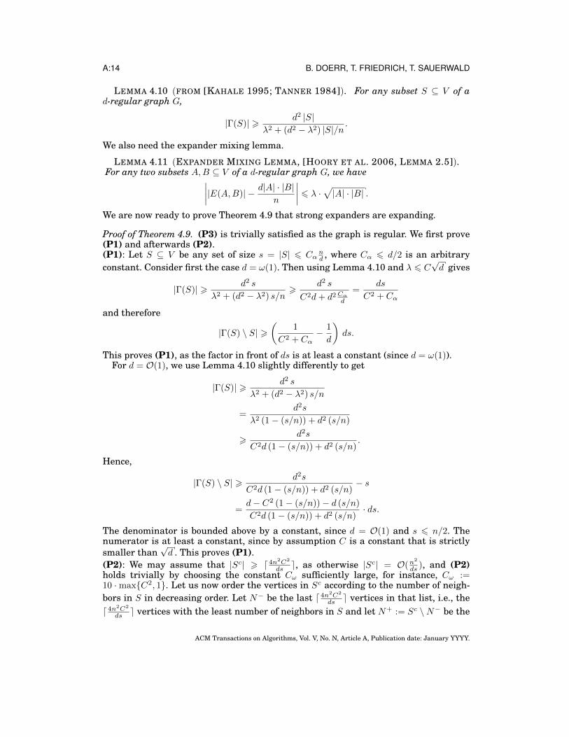
LEMMA 4.10 (FROM [KAHALE 1995; TANNER 1984]). For any subset S ⊆ V of ad-regular graph G,
|Γ(S)| > d2 |S|λ2 + (d2 − λ2) |S|/n
.
We also need the expander mixing lemma.
LEMMA 4.11 (EXPANDER MIXING LEMMA, [HOORY ET AL. 2006, LEMMA 2.5]).For any two subsets A,B ⊆ V of a d-regular graph G, we have∣∣∣∣|E(A,B)| − d|A| · |B|
n
∣∣∣∣ 6 λ ·√|A| · |B| .
We are now ready to prove Theorem 4.9 that strong expanders are expanding.
Proof of Theorem 4.9. (P3) is trivially satisfied as the graph is regular. We first prove(P1) and afterwards (P2).(P1): Let S ⊆ V be any set of size s = |S| 6 Cα
nd , where Cα 6 d/2 is an arbitrary
constant. Consider first the case d = ω(1). Then using Lemma 4.10 and λ 6 C√d gives
|Γ(S)| > d2 s
λ2 + (d2 − λ2) s/n>
d2 s
C2d+ d2Cαd
=ds
C2 + Cα
and therefore
|Γ(S) \ S| >(
1
C2 + Cα− 1
d
)ds.
This proves (P1), as the factor in front of ds is at least a constant (since d = ω(1)).For d = O(1), we use Lemma 4.10 slightly differently to get
|Γ(S)| > d2 s
λ2 + (d2 − λ2) s/n
=d2s
λ2 (1− (s/n)) + d2 (s/n)
>d2s
C2d (1− (s/n)) + d2 (s/n).
Hence,
|Γ(S) \ S| > d2s
C2d (1− (s/n)) + d2 (s/n)− s
=d− C2 (1− (s/n))− d (s/n)
C2d (1− (s/n)) + d2 (s/n)· ds.
The denominator is bounded above by a constant, since d = O(1) and s 6 n/2. Thenumerator is at least a constant, since by assumption C is a constant that is strictlysmaller than
√d . This proves (P1).
(P2): We may assume that |Sc| > d 4n2C2
ds e, as otherwise |Sc| = O(n2
ds ), and (P2)holds trivially by choosing the constant Cω sufficiently large, for instance, Cω :=10 ·maxC2, 1. Let us now order the vertices in Sc according to the number of neigh-bors in S in decreasing order. Let N− be the last d 4n2C2
ds e vertices in that list, i.e., thed 4n2C2
ds e vertices with the least number of neighbors in S and let N+ := Sc \N− be the
ACM Transactions on Algorithms, Vol. V, No. N, Article A, Publication date: January YYYY.
Quasirandom Rumor Spreading A:15
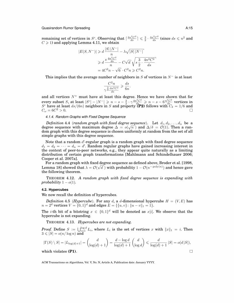
remaining set of vertices in Sc. Observing that d 4n2C2
ds e 632 ·
4n2C2
ds (since ds 6 n2 andC > 1) and applying Lemma 4.11, we obtain
|E(S,N−)| > d|S| |N−|
n− λ√|S| |N−|
> ds 4n2C2
ds
n− C√d
√s
3
2· 4n2C2
ds
= 4C2n−√
6 · C2n > C2n.
This implies that the average number of neighbors in S of vertices in N− is at least
C2n
γ32 ·4n2C2
ds
>ds
6n.
and all vertices N+ must have at least this degree. Hence we have shown that forevery subset S, at least |Sc| − |N−| > n − s − 3
2 · γ4n2C2
ds > n − s − 6n2C2
ds vertices inSc have at least ds/(6n) neighbors in S and property (P2) follows with Cδ = 1/6 andCω = 6C2 > 0.
4.1.4. Random Graphs with Fixed Degree Sequence
Definition 4.4 (random graph with fixed degree sequence). Let d1, d2, . . . , dn be adegree sequence with maximum degree ∆ = o(
√n ) and ∆/δ = O(1). Then a ran-
dom graph with this degree sequence is chosen uniformly at random from the set of allsimple graphs with this degree sequence.
Note that a random d′-regular graph is a random graph with fixed degree sequenced1 = d2 = · · · = dn = d′. Random regular graphs have gained increasing interest inthe context of peer-to-peer networks, e.g., they appear quite naturally as a limitingdistribution of certain graph transformations [Mahlmann and Schindelhauer 2006;Cooper et al. 2007a].
For a random graph with fixed degree sequence as defined above, Broder et al. [1998,Lemma 18] showed that λ = O(
√d ) with probability 1−O(n− poly(n)) and hence gave
the following theorem.
THEOREM 4.12. A random graph with fixed degree sequence is expanding withprobability 1− o(1).
4.2. HypercubesWe now recall the definition of hypercubes.
Definition 4.5 (Hypercube). For any d, a d-dimensional hypercube H = (V,E) hasn = 2d vertices V = 0, 1d and edges E = u, v : ‖u− v‖1 = 1.The i-th bit of a bitstring x ∈ 0, 1d will be denoted as x[i]. We observe that thehypercube is not expanding.
THEOREM 4.13. Hypercubes are not expanding.
Proof. Define S :=⋃log di=1 Li, where Li is the set of vertices x with ‖x‖1 = i. Then
3 6 |S| = o(n/ log n) and
|Γ(S) \ S| = |Llog(d)+1| =(
d
log(d) + 1
)=
d− log d
log(d) + 1
(d
log d
)6
d
log(d) + 1|S| = o(d |S|),
which violates (P1).
ACM Transactions on Algorithms, Vol. V, No. N, Article A, Publication date: January YYYY.
A:16 B. DOERR, T. FRIEDRICH, T. SAUERWALD
Hence a separate analysis is needed, and this is given in Section 7.
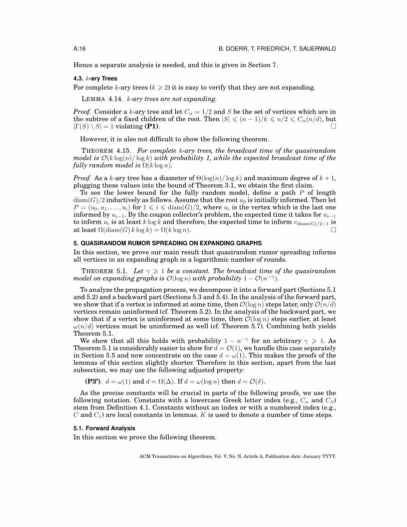
4.3. k-ary TreesFor complete k-ary trees (k > 2) it is easy to verify that they are not expanding.
LEMMA 4.14. k-ary trees are not expanding.
Proof. Consider a k-ary tree and let Cα = 1/2 and S be the set of vertices which are inthe subtree of a fixed children of the root. Then |S| 6 (n − 1)/k 6 n/2 6 Cα(n/d), but|Γ(S) \ S| = 1 violating (P1).
However, it is also not difficult to show the following theorem.
THEOREM 4.15. For complete k-ary trees, the broadcast time of the quasirandommodel is O(k log(n)/ log k) with probability 1, while the expected broadcast time of thefully random model is Ω(k log n).
Proof. As a k-ary tree has a diameter of Θ(log(n)/ log k) and maximum degree of k + 1,plugging these values into the bound of Theorem 3.1, we obtain the first claim.
To see the lower bound for the fully random model, define a path P of lengthdiam(G)/2 inductively as follows. Assume that the root u0 is initially informed. Then letP = (u0, u1, . . . , ui) for 1 6 i 6 diam(G)/2, where ui is the vertex which is the last oneinformed by ui−1. By the coupon collector’s problem, the expected time it takes for ui−1
to inform ui is at least k log k and therefore, the expected time to inform vdiam(G)/2−1 isat least Ω(diam(G) k log k) = Ω(k log n).
5. QUASIRANDOM RUMOR SPREADING ON EXPANDING GRAPHSIn this section, we prove our main result that quasirandom rumor spreading informsall vertices in an expanding graph in a logarithmic number of rounds.
THEOREM 5.1. Let γ > 1 be a constant. The broadcast time of the quasirandommodel on expanding graphs is O(log n) with probability 1−O(n−γ).
To analyze the propagation process, we decompose it into a forward part (Sections 5.1and 5.2) and a backward part (Sections 5.3 and 5.4). In the analysis of the forward part,we show that if a vertex is informed at some time, thenO(log n) steps later, onlyO(n/d)vertices remain uninformed (cf. Theorem 5.2). In the analysis of the backward part, weshow that if a vertex is uninformed at some time, then O(log n) steps earlier, at leastω(n/d) vertices must be uninformed as well (cf. Theorem 5.7). Combining both yieldsTheorem 5.1.
We show that all this holds with probability 1 − n−γ for an arbitrary γ > 1. AsTheorem 5.1 is considerably easier to show for d = O(1), we handle this case separatelyin Section 5.5 and now concentrate on the case d = ω(1). This makes the proofs of thelemmas of this section slightly shorter. Therefore in this section, apart from the lastsubsection, we may use the following adjusted property:
(P3’). d = ω(1) and d = Ω(∆). If d = ω(log n) then d = O(δ).
As the precise constants will be crucial in parts of the following proofs, we use thefollowing notation. Constants with a lowercase Greek letter index (e.g., Cα and Cβ)stem from Definition 4.1. Constants without an index or with a numbered index (e.g.,C and C1) are local constants in lemmas. K is used to denote a number of time steps.
5.1. Forward AnalysisIn this section we prove the following theorem.
ACM Transactions on Algorithms, Vol. V, No. N, Article A, Publication date: January YYYY.
Quasirandom Rumor Spreading A:17
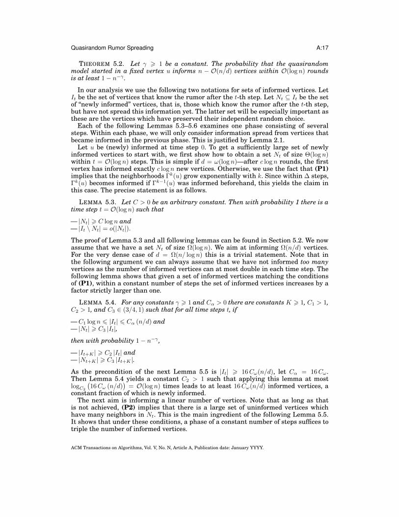
THEOREM 5.2. Let γ > 1 be a constant. The probability that the quasirandommodel started in a fixed vertex u informs n − O(n/d) vertices within O(log n) roundsis at least 1− n−γ .
In our analysis we use the following two notations for sets of informed vertices. LetIt be the set of vertices that know the rumor after the t-th step. Let Nt ⊆ It be the setof “newly informed” vertices, that is, those which know the rumor after the t-th step,but have not spread this information yet. The latter set will be especially important asthese are the vertices which have preserved their independent random choice.
Each of the following Lemmas 5.3–5.6 examines one phase consisting of severalsteps. Within each phase, we will only consider information spread from vertices thatbecame informed in the previous phase. This is justified by Lemma 2.1.
Let u be (newly) informed at time step 0. To get a sufficiently large set of newlyinformed vertices to start with, we first show how to obtain a set Nt of size Θ(log n)within t = O(log n) steps. This is simple if d = ω(log n)—after c log n rounds, the firstvertex has informed exactly c log n new vertices. Otherwise, we use the fact that (P1)implies that the neighborhoods Γk(u) grow exponentially with k. Since within ∆ steps,Γk(u) becomes informed if Γk−1(u) was informed beforehand, this yields the claim inthis case. The precise statement is as follows.
LEMMA 5.3. Let C > 0 be an arbitrary constant. Then with probability 1 there is atime step t = O(log n) such that
— |Nt| > C log n and— |It \Nt| = o(|Nt|).
The proof of Lemma 5.3 and all following lemmas can be found in Section 5.2. We nowassume that we have a set Nt of size Ω(log n). We aim at informing Ω(n/d) vertices.For the very dense case of d = Ω(n/ log n) this is a trivial statement. Note that inthe following argument we can always assume that we have not informed too manyvertices as the number of informed vertices can at most double in each time step. Thefollowing lemma shows that given a set of informed vertices matching the conditionsof (P1), within a constant number of steps the set of informed vertices increases by afactor strictly larger than one.
LEMMA 5.4. For any constants γ > 1 and Cα > 0 there are constants K > 1, C1 > 1,C2 > 1, and C3 ∈ (3/4, 1) such that for all time steps t, if
—C1 log n 6 |It| 6 Cα (n/d) and— |Nt| > C3 |It|,
then with probability 1− n−γ ,
— |It+K | > C2 |It| and— |Nt+K | > C3 |It+K |.
As the precondition of the next Lemma 5.5 is |It| > 16Cω(n/d), let Cα = 16Cω.Then Lemma 5.4 yields a constant C2 > 1 such that applying this lemma at mostlogC2
(16Cω (n/d)
)= O(log n) times leads to at least 16Cω(n/d) informed vertices, a
constant fraction of which is newly informed.The next aim is informing a linear number of vertices. Note that as long as that
is not achieved, (P2) implies that there is a large set of uninformed vertices whichhave many neighbors in Nt. This is the main ingredient of the following Lemma 5.5.It shows that under these conditions, a phase of a constant number of steps suffices totriple the number of informed vertices.
ACM Transactions on Algorithms, Vol. V, No. N, Article A, Publication date: January YYYY.
A:18 B. DOERR, T. FRIEDRICH, T. SAUERWALD
LEMMA 5.5. For any constant γ > 1 there are constants K > 1, C > 1, and Cω > 0such that for all time steps t, if
— maxC log n, 16Cω(n/d) 6 |It| 6 n/16 and— |Nt| > (3/4) |It|,
then with probability 1− n−γ ,
— |It+K | > 3 |It| and— |Nt+K | > (3/4) |It+K |.
Applying Lemma 5.5 at most O(log n) times, a linear fraction of the vertices gets in-formed. In a final phase of O(log n) steps, one can then inform all but O(n/d) verticesas shown in the following Lemma 5.6.
LEMMA 5.6. For any constants γ > 1 and C > 0 there is a K = O(log n) such thatfor all time steps t, if
— |Nt| > C n,
then with probability 1− n−γ ,
— |It+K | = n−O(n/d).
Combining all above phases, a union bound gives |IO(logn)| = n−O(n/d) with prob-ability 1−O(log(n)n−γ). As γ was arbitrary in all lemmas, Theorem 5.2 follows.
5.2. Proofs of the Lemmas Used in the Forward AnalysisProof of Lemma 5.3. Let u be informed at time step 0. If d = ω(log n), then by (P3)δ = Θ(d) and a single phase of C log n rounds suffices, that is, we haveNC logn = C log n,and the lemma follows.
We now describe how to obtain C log n newly informed vertices for d = O(log n). Forthis, we choose a Cα such that Cαn/d > C log n and get, by (P1) for k > 3, as long as|Γ6k(v)| = O(n/d),
|Γ6k+1(v)| = |Γ6k(v)|+ |Γk+1(v)| = |Γ6k(v)|+ |Γ(Γ6k(v)) \ Γ6k(v)|> (1 + Cβd) |Γ6k(v)|. (1)
Subtracting |Γ6k(v)| on both sides yields
|Γk+1(v)| > Cβ d |Γ6k(v)|.
As |Γ63(v)| > 3, by induction,
|Γk(v)| > 3 (Cβ d)k−3
for all k with k > 3 and |Γ6k−1(v)| 6 C log n. Therefore we can choose a k =O(log log(n)/ log d) such that |Γk(v)| > C log n.
We use the delaying and ignoring assumption (cf. Lemma 2.1) to perform k phasesof ∆ rounds each. Then after these t = ∆k = O(∆ (log log n)/ log d) = O(log n) steps(as ∆ = O(d) by (P3) and d/ log d = O(log(n)/ log log n) by d = O(log n)) all vertices inΓ6k(v) get informed, but no vertex of Γk(v) has been active. In consequence, we have
|Nt| = |Γk(v)| > C log n, (2)
|It \Nt| = |Γ6k−1(v)| 6 |Γk(v)|/(Cβ d) = o(|Nt|),where the last equation stems from (P3’).
ACM Transactions on Algorithms, Vol. V, No. N, Article A, Publication date: January YYYY.
Quasirandom Rumor Spreading A:19
Proof of Lemma 5.4. We choose the following constants:
C1 := 8 γ∆2
C2β d
2 > 1, C2 := 4 ∆Cβ d
> 1,
C3 :=(
1− Cβ d4 ∆
)∈ (3/4, 1), K :=
⌈(3 ∆Cβ d
)2⌉> 1,
where the Cβ is from (P1) and depends on the given Cα. K and C1 to C3 are all Θ(1)by (P3). As It is a connected set of appropriate size, (P1) gives
|Γ(It) \ It| > Cβ d |It|. (3)
Since we are interested in the expansion of Nt and not of It, we calculate
|Γ(It) \ It| =∣∣(Γ(It \Nt) \ It
)∪(Γ(Nt) \ It
)∣∣6∣∣Γ(It \Nt) \ It
∣∣+∣∣Γ(Nt) \ It
∣∣6 ∆|It \Nt|+
∣∣Γ(Nt) \ It∣∣. (4)
Combining equations (3) and (4) with the assumption |It \Nt| 6 Cβ d4 ∆ |It|,∣∣Γ(Nt) \ It
∣∣ > Cβ d |It| −∆|It \Nt| > 3Cβ d |It|/4.We now perform one phase consisting ofK rounds. We compute the size of the resultingsets It+K and Nt+K as follows.
Let v ∈ Γ(Nt) \ It. Then there is a u ∈ Nt such that (u, v) ∈ E. The probability that ucontacts v within this time interval is minK/deg(u), 1 > K/∆ (as ∆ = ω(1) by (P3’)),which naturally is a lower bound for v becoming contacted by an arbitrary vertex ofNt. By linearity of expectation, the expected number of vertices becoming contacted isat least
E [|Nt+K |] > K |Γ(Nt) \ It|/∆ > 3CβK d |It|/(4∆).
As every vertex can only contact at most K vertices in this time interval, Azuma’sinequality (cf. Lemma A.2) gives a probabilistic lower bound on the number of newlyinformed vertices. More precisely,
Pr
[|Nt+K | 6
CβK d |It|2∆
]6 exp
(−C2β d
2 |It|2
8 ∆2 |Nt|
)6 n−C1 C
2β d
2/(8 ∆2) = n−γ .
It remains to check that |Nt+K | > Cβ K d |It|2 ∆ implies the two parts of the claim. First,
|It+K | > |Nt+K | >CβK d
2 ∆|It| >
4 ∆
Cβ d|It| = C2 |It|.
For the second part, observe that
|Nt+K | >CβK d |It|
2 ∆>CβK d (|It+K | − |Nt+K |)
2 ∆=CβK d
2 ∆|It+K | −
CβK d
2 ∆|Nt+K |.
Rearranging yields
|Nt+K | >CβK d
2 ∆ + CβK d|It+K | >
Cβ(
3 ∆Cβ d
)2d
2∆ + Cβ(
3 ∆Cβ d
)2d|It+K |
=9∆
2Cβ d+ 9 ∆|It+K | >
(1− Cβ d
4 ∆
)|It+K |.
ACM Transactions on Algorithms, Vol. V, No. N, Article A, Publication date: January YYYY.
A:20 B. DOERR, T. FRIEDRICH, T. SAUERWALD
Proof of Lemma 5.5. We choose C := 512 γ3 ∆2
3C2δ d
2 > 1, K :=⌈
16 γ∆Cδ d
⌉> 1, and Cω > 0
according to (P2).By property (P2), the number of vertices in N c
t which have at least Cδd |Nt|/n neigh-bors in Nt is at least |N c
t | − Cω n2
d |Nt| . Therefore, the number of vertices in Ict which haveat least Cδd(|Nt|/n) neighbors in Nt is at least
|N ct | − |It| − Cω n
2
d |Nt| > n− 2 |It| − n/12 > 19n/24 > 3n/4,
where the first inequality is due to 16Cω(n/d) 6 |It| 6 4/3 |Nt|.We call a vertex v ∈ Ict good if it has at least Cδd |Nt|/n neighbors in Nt. The probabilitythat a good vertex gets informed in a phase of K rounds (again using K 6 ∆ = ω(1) by(P3’)) is at least
1−(
1− K
∆
)Cδd |Nt|/n> 1− exp
(− KCδd |Nt|
∆n
)> 1− exp(−16 γ |Nt|/n)
> 1− 1(16 γ |Nt|/n)+1 = 16 γ |Nt|
16 γ |Nt|+n .
By linearity of expectation,
E [|Nt+K |] > 16 γ |Nt|16 γ |Nt|+n
3n4 > 16 γ |Nt|
16 γ n/16+n3n4 = γ |Nt|
(γ/16)+1/1634 > 6 |Nt|.
Azuma’s inequality (cf. Lemma A.2) gives
Pr [|Nt+K | 6 4 |Nt|] 6 exp
(−2 (2|Nt|)2
|Nt|K2
)= exp
(−8|Nt|
K2
)6 exp
(−|Nt|C
2δ d
2
128 γ2∆2
)6 exp
(−3C log(n)C2
δ d2
512 γ2∆2
)= n−γ .
Therefore with probability 1− n−γ ,
|Nt+K | > 4 |Nt| > 3 |It| = 3 |It+K | − 3 |Nt+K |
and after rearranging,
|Nt+K | > 34 |It+K |.
This proves the first claim. The second claim follows from
|It+K | > |Nt+K | > 4|Nt| > 3 |It|.
Proof of Lemma 5.6. Let X ⊆ N ct be the set of vertices in N c
t that have at leastCδ d |Nt|/n neighbors in Nt. By (P2),
|X| > (n− |Nt|)−Cω n
2
d|Nt|> n− |Nt| −Θ
(nd
).
Let v ∈ X and consider a phase of K :=⌈
2 γ∆nCδ |Nt| d log n
⌉rounds. Note that K = O(log n)
by (P3).If K > ∆, v becomes informed in this phase with probability 1. Otherwise, the prob-
ability that v will not be informed in this phase is at most
Pr [v /∈ Nt+K ] 6
(1− K
∆
)Cδ|Nt|d/n6 exp(−2 γ log n) = n−2 γ .
ACM Transactions on Algorithms, Vol. V, No. N, Article A, Publication date: January YYYY.
Quasirandom Rumor Spreading A:21
Taking the union bound over all vertices in X, we obtain that all vertices in X getinformed with probability 1− n−γ . The claim follows.
5.3. Backward AnalysisThe forward analysis has shown that within O(log n) steps, at most O(n/d) verticesstay uninformed. We now analyze the reverse. The question here is how many verticeshave to be uninformed at time t − O(log n) if there is an uninformed vertex at time t.We will show that this is at least ω(n/d). To formalize this, recall that U[t1,t2](w) is theset of vertices that reach the vertex w within the time interval [t1, t2] (using the usualmeaning of “reach” as defined on page 7). We will prove the following theorem.
THEOREM 5.7. Let γ > 1 be a constant. If the quasirandom rumor spreading pro-cess does not inform a fixed vertex w until some time t, then there are ω(n/d) uninformedvertices at time t−O(log n) with probability at least 1− n−γ .
To prove Theorem 5.7, we fix an arbitrary vertex w and a time t. Ignoring sometechnicalities, our aim is to prove a lower bound on the number of vertices which haveto be uninformed at times before t to keep w uninformed at time t. We first show thatthe set of uninformed vertices at time t−O(log n) is at least of logarithmic size.
For d = O(log n) this follows from (P1) as all vertices of ΓO(log logn/ log d)(w) (andthere are at least Ω(log n) of these) reach w within O(log n) steps. For d = ω(log n), asimple Chernoff bound shows that enough vertices of Γ(w) contact w within O(log n)steps. This is summarized in the following lemma. The proofs of all three lemmas ofthis section can be found in the following Section 5.4.
LEMMA 5.8. Let γ > 1 and C > 1 be constants, w a vertex, and t2 = Ω(log n) a timestep. Then with probability 1− 2n−γ there is a time step t1 = t2 −O(log n) such that
|U[t1,t2](w)| > C log n.
We now know that within a logarithmic number of time steps, there are at least c log nvertices which have reached w. Very similarly to Lemmas 5.4 and 5.5 in the forwardanalysis, we can increase the set of vertices that reach w by a multiplicative factorby going back a constant number of time steps. The following lemma again mainlyuses (P1). For the very dense case of d = Ω(n/ log n), there is nothing to show.
LEMMA 5.9. For any constant γ > 1 there is a constantK such that for all vertices wand time steps t1, t2, if
log n 6 |U[t1,t2](w)| = O(n/d),
then with probability 1− n−γ ,
|U[t1−K,t2](w)| > 4 |U[t1,t2](w)|.
Using Lemma 5.9 at mostO(log n) times, we obtain a set of vertices that reach w of sizeΩ(n/d). If these are ω(n/d) vertices, we are done. Otherwise, the following Lemma 5.10shows that a phase consisting of O(log n) steps suffices to get to this point. This is theonly lemma which substantially uses (P3’).
LEMMA 5.10. Let γ > 1 be a constant, w a vertex, and t1, t2 time steps such that
|U[t1,t2](w)| = Θ(n/d).
Then with probability 1− n−γ ,
|U[t1−O(logn),t2](w)| = ω(n/d).
ACM Transactions on Algorithms, Vol. V, No. N, Article A, Publication date: January YYYY.
A:22 B. DOERR, T. FRIEDRICH, T. SAUERWALD
This finishes the backward analysis and shows that ω(n/d) vertices have to be unin-formed to keep a single vertex uninformed forO(log n) steps. Together with the forwardanalysis, which proved that only O(n/d) vertices remain uninformed after O(log n)steps, this finishes the proof of Theorem 5.1 for d = ω(1).
5.4. Proofs of the Lemmas Used in the Backward AnalysisProof of Lemma 5.8. Consider first the case that d = O(log n). In this case, we choose,as in the proof of Lemma 5.3, a constant Cα such that Cαn/d > C log n and apply (P1).By equation (2) from page 18, there exists a k = O(log log(n)/ log d) such that
|Γ6k(w)| > |Γk(w)| > C log n.
Since within ∆ rounds each vertex has contacted all neighbors, we have Γ6i(w) ⊆U[t2−i∆,t2](w) for i > 1 and therefore Γ6k(w) ⊆ U[t2−k∆,t2](w). As k∆ = O(log n), we seethat |U[t2−O(logn),t2]| > C log n with probability 1.
In the remaining case d = ω(log n) we estimate the number of neighbors of w whichreach w in the previous K := d4C2γ∆ log(n)/δe steps. Note that K = O(log n) by(P3). For each neighbor u ∈ Γ(w), define a random variable X(u), which is one ifu contacts v within the time interval [t2 − K, t2], and zero otherwise. Then for eachu ∈ Γ(w), Pr [X(u) = 1] > K/∆. We define X :=
∑u∈Γ(w)Xu. Linearity of expectation
gives E [X] > K δ/∆ > 4C2γ log n. Since X(u) : u ∈ Γ(w) is a set of independentrandom variables, we obtain by a Chernoff bound that
Pr [X 6 C log n] 6 Pr[X 6 1
4 E [X]]
6 exp(−(3/4)2 E [X] /2
)= exp
(−(9/32) 4C2γ log n
)6 n−γ ,
where we used the assumption C > 1. This implies that with probability 1 − n−γ , wehave ∣∣U[t2−O(logn),t2](w)
∣∣ > C log n.
Proof of Lemma 5.9. Let S := U[t1,t2](w) and let |S| 6 Cα (n/d) for a constant Cα. As Sis a connected set, (P1) gives
|Γ(S) \ S| > Cβ d |S|.
for a suitable constant Cβ . Let K =⌈
8 γCβ
∆d
⌉= O(1) (by (P3)). As every vertex u ∈
Γ(S)\S has at least one edge to a vertex v ∈ S, the probability that a vertex u ∈ Γ(S)\Scontacts a v ∈ S in the interval [t1 −K, t1 − 1] is at least K/∆ and S′ := U[t1−K,t2](w).By linearity of expectation, the expected number of vertices in S′ \ S is at least
E [|S′ \ S|] > K|Γ(S) \ S|/∆ > CβKd |S|/∆.A simple application of the Chernoff bound gives
Pr
[|S′ \ S| 6 CβKd |S|
2∆
]6 exp
(−CβKd |S|
8∆
)6 n−
CβKd
8∆ .
Hence with probability 1− n−γ ,
|S′| > CβKd |S|2∆
> 4γ|S| > 4 |S|.
ACM Transactions on Algorithms, Vol. V, No. N, Article A, Publication date: January YYYY.
Quasirandom Rumor Spreading A:23
Proof of Lemma 5.10. Let S := U[t1,t2](w) with |S| 6 Cα (n/d) for a constant Cα. Alsolet K :=
⌈8γCβ
∆d
n|S| d log n
⌉and S′ := U[t1−K,t2](w). Note that K = O(log n) by (P3). We
examine a phase of K steps.As S is a connected set, (P1) gives, as in the proof of Lemma 5.9, |Γ(S)\S| > Cβ d |S|.
If K > ∆, the lemma immediately follows from the observation
|S′| = |Γ61(S)| = Θ(d |S|) = Θ(n) = ω(n/d).
The last equality is based on d = ω(1) as given by (P3’).We now assume K 6 ∆. As every vertex u ∈ Γ(S) \ S has at least one edge to a
vertex v ∈ S, the probability that a vertex u ∈ Γ(S) \ S contacts a v ∈ S in the interval[t1 − K, t1 − 1] is at least K/∆. By linearity of expectation, the expected number ofvertices in S′ \ S is at least
K
∆|Γ(S) \ S| > CβKd |S|
∆>
8γ n log n
d
Again, a Chernoff bound gives
Pr
[|S′ \ S| 6 4γ n log n
d
]6 exp
(−γ n log n
d
)6 n−γ .
Hence |S′| > |S′ \ S| = Ω(n log(n)/d) = ω(n/d) with probability 1− n−γ for K 6 ∆.
5.5. Analysis for Graphs with Constant DegreeIt remains to show that the quasirandom model also works well on expanding graphswith constant degree d = O(1). To do this, we apply Theorem 3.1 to see that for anygraph the quasirandom model succeeds in ∆ · diam(G) steps. The corresponding boundfor the fully random model is O(∆ (diam(G) + log n)) with probability 1 − n−1 [Feigeet al. 1990, Theorem 2.2].
Naturally, the diameter of expanding graphs can be bounded easily as follows(cf. [Hoory et al. 2006, p. 455] for a related result). Plugging Lemma 5.11 into theupper bound of ∆ · diam(G) yields Theorem 5.1 for d = O(1).
LEMMA 5.11. For any expanding graph G with d = O(1), diam(G) = O(log n).
Proof. Fix two vertices v and w. We show that Γ6O(logn)(v) ∪ Γ6O(logn)(w) 6= ∅. As G isconnected, |Γ63(v)| > 3. Now we choose Cα = d/2 (which is valid since d is a constant)and proceed as in the proof of Lemma 5.3. By (P1) we again get equation (1) for k > 3,and therefore by induction
|Γ6k(v)| > 3 (1 + Cβd)k−3
for all k with k > 3 and |Γ6k−1(v)| 6 n/2. Therefore we can choose a k such that|Γ6k(v)| > n/2 and k = O(log n). As analogously |ΓO(logn)(w)| > n/2, we can concludethat there is a path of length O(log n) from v to w.
6. LOWER BOUNDS FOR THE FULLY RANDOM MODEL ON SPARSE RANDOM GRAPHSIn this section, we discuss lower bounds for the fully random model on sparse randomgraphs. They will show that the quasirandom model is superior on such graphs. Feigeet al. [1990] proved the following bound.
THEOREM 6.1 ([FEIGE ET AL. 1990, THEOREM 4.1]). Let p = (log n + f(n))/n,where f(n) = ω(1) and f(n) = O(log log n). Then for almost all random graphs G(n, p),the broadcast time of the fully random model is Ω(log2 n) with probability at least n−1.
ACM Transactions on Algorithms, Vol. V, No. N, Article A, Publication date: January YYYY.
A:24 B. DOERR, T. FRIEDRICH, T. SAUERWALD
Broadcast timeRandom model Quasirandom model
O(log2 n) with probability > 1− n−1 [Feige et al. 1990] O(logn) with probability > 1− n−γ ∀γ = O(1)
(Thm. 4.2 and 5.1)Ω(log2 n) with probability > n−1 [Feige et al. 1990]
Ω(log(n) log logn) with probability > 1− o(1) (Thm. 6.2)
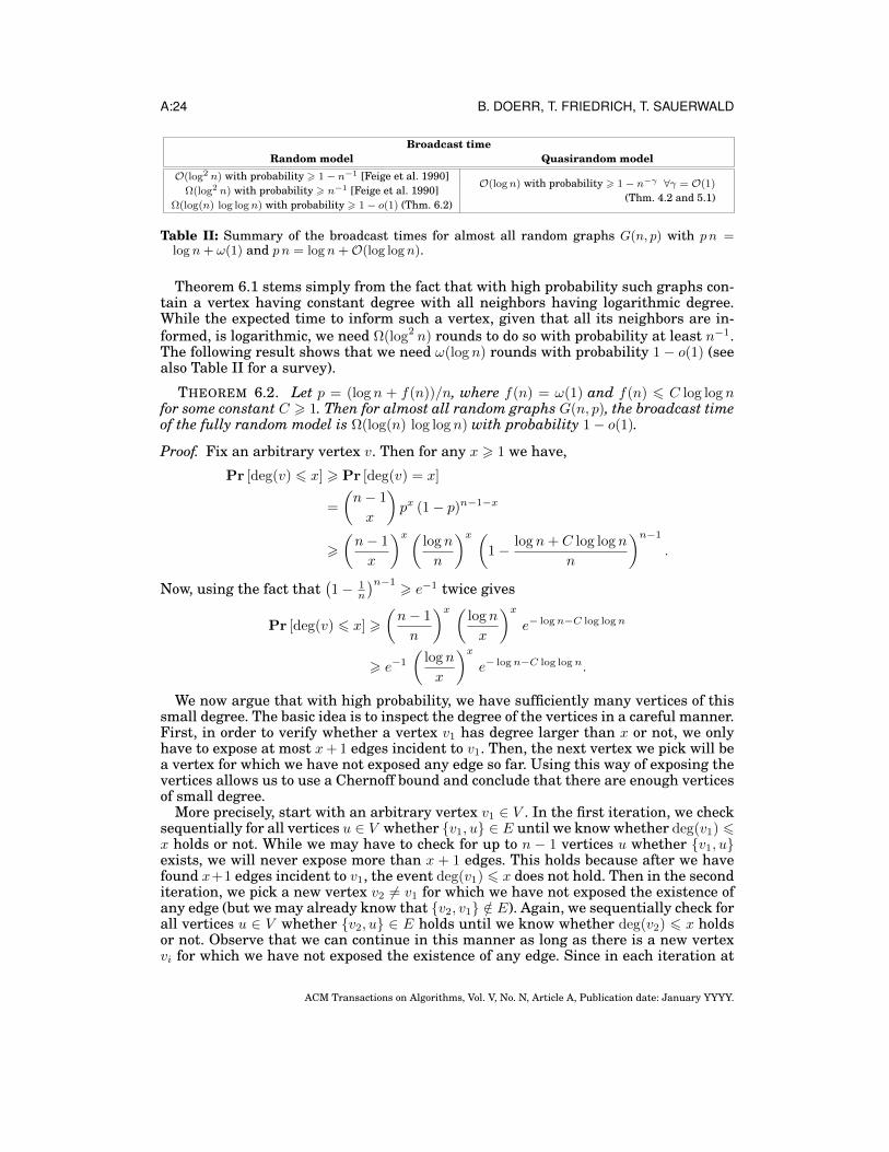
Table II: Summary of the broadcast times for almost all random graphs G(n, p) with p n =logn + ω(1) and p n = logn +O(log logn).
Theorem 6.1 stems simply from the fact that with high probability such graphs con-tain a vertex having constant degree with all neighbors having logarithmic degree.While the expected time to inform such a vertex, given that all its neighbors are in-formed, is logarithmic, we need Ω(log2 n) rounds to do so with probability at least n−1.The following result shows that we need ω(log n) rounds with probability 1− o(1) (seealso Table II for a survey).
THEOREM 6.2. Let p = (log n + f(n))/n, where f(n) = ω(1) and f(n) 6 C log log nfor some constant C > 1. Then for almost all random graphs G(n, p), the broadcast timeof the fully random model is Ω(log(n) log log n) with probability 1− o(1).
Proof. Fix an arbitrary vertex v. Then for any x > 1 we have,
Pr [deg(v) 6 x] > Pr [deg(v) = x]
=
(n− 1
x
)px (1− p)n−1−x
>
(n− 1
x
)x(log n
n
)x (1− log n+ C log log n
n
)n−1
.
Now, using the fact that(1− 1
n
)n−1> e−1 twice gives
Pr [deg(v) 6 x] >
(n− 1
n
)x (log n
x
)xe− logn−C log logn
> e−1
(log n
x
)xe− logn−C log logn.
We now argue that with high probability, we have sufficiently many vertices of thissmall degree. The basic idea is to inspect the degree of the vertices in a careful manner.First, in order to verify whether a vertex v1 has degree larger than x or not, we onlyhave to expose at most x+ 1 edges incident to v1. Then, the next vertex we pick will bea vertex for which we have not exposed any edge so far. Using this way of exposing thevertices allows us to use a Chernoff bound and conclude that there are enough verticesof small degree.
More precisely, start with an arbitrary vertex v1 ∈ V . In the first iteration, we checksequentially for all vertices u ∈ V whether v1, u ∈ E until we know whether deg(v1) 6x holds or not. While we may have to check for up to n − 1 vertices u whether v1, uexists, we will never expose more than x + 1 edges. This holds because after we havefound x+1 edges incident to v1, the event deg(v1) 6 x does not hold. Then in the seconditeration, we pick a new vertex v2 6= v1 for which we have not exposed the existence ofany edge (but we may already know that v2, v1 /∈ E). Again, we sequentially check forall vertices u ∈ V whether v2, u ∈ E holds until we know whether deg(v2) 6 x holdsor not. Observe that we can continue in this manner as long as there is a new vertexvi for which we have not exposed the existence of any edge. Since in each iteration at
ACM Transactions on Algorithms, Vol. V, No. N, Article A, Publication date: January YYYY.
Quasirandom Rumor Spreading A:25
most x + 1 edges are exposed, the number of vertices with no exposed edge is reducedby at most x+ 2 per iteration. As a consequence, the whole procedure can be run for atleast n/(x+ 2) iterations. In each iteration 1 6 i 6 n/(x+ 2), we have
Pr [deg(vi) 6 x] > e−1
(log n
x
)xe− logn−C log logn,
by the same reasoning as above.Let X be the number of vertices with degree at most x. By the arguments above, it
follows thatX is stochastically larger (cf. Definition A.1 for a definition of stochasticallylarger) than the sum of n/(x + 2) independent Bernoulli-random variables each ofwhich has success probability e−1
(lognx
)xe− logn−C log logn. Therefore, it follows by a
Chernoff bound (Lemma A.1) that
Pr[X 6 1
2 E [X]]6 e−(1/2)2 E[X]/2. (5)
Now choose x := (log n)ε for an arbitrary constant 0 < ε < 1. By the above, we obtain
E [X] >n
(log n)ε + 2e−1
(log n
(log n)ε
)(logn)ε
e− logn−C log logn
> 13 (log n)−ε−C+(1−ε)(logn)ε = (log n)
Ω((logn)ε).
Plugging this into equation (5), we obtain
Pr[X 6 (log n)Ω((logn)ε)
]= o(1).
By [Cooper and Frieze 2007, Lemma 1, Property 2] we know that for almost all randomgraphs, any two vertices with a degree of less than log n/20 have a distance of at leastlog n/(log log n)2 from each other. Hence, all neighbors of vertices in X have a degreeof more than log n/20. In particular, the time until a vertex u ∈ X gets contacted bya fixed neighbor v ∈ N(u) is stochastically larger than a geometric random variablewith parameter log n/20. Hence the time until u gets contacted by any of its neighborsis stochastically larger than the minimum of deg(u) 6 x = (log n)ε independent suchgeometric variables. Since any two vertices in X have a distance of at least three, thesetimes are independent for all u ∈ X.
Now recall that R(G) is the random variable describing the runtime of thefully random model. Further, let Geo(p) be the geometric distribution defined byPr [Geo(p) = i] = p · (1 − p)i for any integer i > 0. Denoting with “stochasticallylarger” and using Lemma A.4, we obtain
R(G) maxu∈X
minv∈N(x)
Geo(20/ log n)
maxu∈X
Geo
1−∏
v∈N(x)
(1− 20/ log n)
max
u∈X
Geo
(1− (1− 20/ log n)(logn)ε
)
(logn)Ω((logn)ε)
maxi=1
Geo
(1− e−20(logn)ε−1
).
ACM Transactions on Algorithms, Vol. V, No. N, Article A, Publication date: January YYYY.
A:26 B. DOERR, T. FRIEDRICH, T. SAUERWALD
Hence
Pr [R(G) 6 t] 6 Pr[Geo
(1− e−20(logn)ε−1
)6 t](logn)Ω((logn)ε)
=
(1−
(e−20(logn)ε−1
)t)(logn)Ω((logn)ε)
6 exp(−e−20(logn)ε−1t (log n)Ω((logn)ε)
).
Setting t = c log n log log n with a sufficiently small constant c finally gives
Pr [R(G) 6 t] 6 exp(−(log n)−20c(logn)ε (log n)Ω((logn)ε)
)= exp
(−(log n)Ω((logn)ε)
).
7. QUASIRANDOM RUMOR SPREADING ON HYPERCUBESIn this section we analyze the quasirandom model on hypercubes. We prove that thequasirandom model informs all vertices in O(log n) rounds with high probability. Thisextends a corresponding runtime bound ofO(log n) for the fully random model in [Feigeet al. 1990]. The difficulty in our analysis is that the hypercube is not an expandinggraph (cf. Theorem 4.13), and also an application of the bound of Theorem 3.1 yieldsonly a much weaker upper bound of O(log2 n).
We now state and prove our runtime bound for the quasirandom model on hyper-cubes. Finally, we will also examine the failure probability more closely to reveal thatthere is again a slight superiority of the quasirandom model over the fully randommodel (Section 7.4).
THEOREM 7.1. The broadcast time of the quasirandom model on the hypercube isO(log n) with probability 1− n−Ω(logn).
Similarly to the proof for expanding graphs in Section 5, the analysis consists ofa forward part and backward part. While the analysis of the forward part borrowsseveral concepts from the analysis of the fully random model [Feige et al. 1990], theidea of analyzing the process in reversed order was not used in [Feige et al. 1990].
The forward part informs sufficiently many vertices in O(log n) time. The backwardpart shows that if there is an uninformed vertex, then O(log n) steps earlier every ballof small radius in the hypercube contains at least one uninformed vertex. To provethat one of these uninformed vertices gets informed eventually, we need a third partin between, which we call coupling. A graphical illustration of our proof can be foundin Figure 1 on page 30.
To formally prove Theorem 7.1, we assume that the following three lemmas hold. Westate them here and prove them in the remainder of this section. Recall that n = 2d.
LEMMA 7.2. The probability that the quasirandom rumor spreading process startedin a fixed vertex s informs 2d/6 vertices in 3d steps is at least 1− n−Ω(logn).
Let s = 0d be initially informed. By Lemma 7.2, at least 2d/6 vertices get informedin 3d with probability at least 1− n−Ω(logn). Now fix an arbitrary vertex w ∈ V . Recallthat U[t1,t2](w) is the set of vertices that reach the vertex w within the time interval[t1, t2] (cf. definition on page 7).
LEMMA 7.3. For any vertex w and t2 = 1033d, with probability at least 1−n−Ω(logn),there is for every vertex v a vertex u(v) ∈ U[6d,t2](w) with dist(u, v) 6 d/256.
ACM Transactions on Algorithms, Vol. V, No. N, Article A, Publication date: January YYYY.
Quasirandom Rumor Spreading A:27
By applying Lemma 7.3, there is with probability at least 1 − n−Ω(logn) for eachv ∈ I3d a vertex u(v) ∈ U[6d,t2](w) with dist(u, v) 6 d/256.
LEMMA 7.4. Let s be the initially informed vertex and w be an arbitrary vertex.Assume that the following two conditions hold:
— there are at least 2d/6 informed vertices at step 3d and— there is for every vertex v a vertex u(v) ∈ U[6d,t2](w) with dist(u, v) 6 d/256 and t2 =
1033d.
Then with probability 1−e− poly(n), at least one vertex in U[6d,t2](w) is informed at step 6d.
Now if the two former conditions hold, Lemma 7.4 implies that a vertex in U[6d,t2](w)
gets informed with (conditional) probability at least 1 − n−Ω(logn). By definition thisimplies that the vertex w gets informed at step t2. Taking the union bound over thesuccess of the forward and backward part (Lemma 7.2 and Lemma 7.3), it follows thatat step t2 the vertex w gets informed with probability at least 1−n−Ω(logn). Taking theunion bound over all possible vertices w ∈ V yields Theorem 7.1.
7.1. Proof of the Forward AnalysisIn this section we prove Lemma 7.2.
Proof of Lemma 7.2. By symmetry we may assume that s = 0d is initially informed.Let Li be the set of vertices with ‖x‖1 = i. Note that after two phases of d steps each,we have I2d = s ∪ L1 ∪ L2.
Consider some time-step t > 2d. Assume that all initially-contacted neighbors of It ∩Li are still to be chosen u. a. r. for i > 2. Notice that the number of edges between It∩Liand Li+1 is |E(It∩Li, Li+1)| =
∑v∈Li+1
degIt∩Li(v) = |It∩Li| (d− i). Our goal is to showthat a large set of vertices in Li+1 will be informed after a phase of 4 additional steps.The probability that a vertex v ∈ Li+1 is still uninformed after this phase is
Pr [v 6∈ It+4] 6∏
u∈Γ(v)∩It∩Li
(1− 4
d
)=
(1− 4
d
)degIt∩Li (v)
.
By linearity of expectations we get
E [|It+4 ∩ Li+1|] =∑
v∈Li+1
Pr [v ∈ It+4] >∑
v∈Li+1
1−(
1− 4
d
)degIt∩Li (v)
>∑
v∈Li+1
1− exp
(−
4 degIt∩Li(v)
d
).
Let us now assume that 1 6 i 6 d/4− 1. Then since degIt∩Li(v) 6 i+ 1 for v ∈ Li+1 and1 + x
2 > ex for any −1 6 x 6 0, we get
E [|It+4 ∩ Li+1|] >∑
v∈Li+1
2 degIt∩Li(v)
d=
2
d|It ∩ Li| (d− i) = 2
d− id|It ∩ Li|.
ACM Transactions on Algorithms, Vol. V, No. N, Article A, Publication date: January YYYY.
A:28 B. DOERR, T. FRIEDRICH, T. SAUERWALD
Since any vertex of |It ∩Li| can only inform at most 4 vertices within 4 steps, an appli-cation of Azuma’s inequality (cf. Lemma A.2) gives, for any constant 0 < ε 6 2/3,
Pr
[|It+4 ∩ Li+1| 6 (2− ε) d− i
d|It ∩ Li|
]6 exp
(−
(ε d−id |It ∩ Li|)2
16 |It ∩ Li|
)= exp(−Ω(d2)) = n−Ω(logn),
as long as |It ∩ Li| > d (d−1)2 holds. Observe that if the condition |It ∩ Li| > d (d−1)
2 holdsinitially, then |It+4 ∩Li+1| > (2− ε)d−id |It ∩Li| implies that |It+4 ∩Li+1| > d (d−1)
2 , since(2− ε)d−id > (2− ε) 3
4 > 1 by definition of i and ε.Recall that we first spent 2d steps in the first two phases to inform L2 completely.
Then in the analysis above, we spent, for each level i with 2 6 i 6 d/4 − 1, a phase ofexactly 4 steps. Hence the total time consumption is
2d+ (d/4− 2) · 4 6 3d.
Now taking the union bound over all levels 2 6 i 6 d/4− 1, with probability 1− (d/4−1)n−Ω(logn) = 1− n−Ω(logn) it holds that
|I4d ∩ Ld/4| >d (d− 1)
2
d/4−1∏i=2
((2− ε) d− i
d
)
=d (d− 1)
2(2− ε)d/4−2
d/4−1∏i=2
(1− i
d
).
We now use the fact that (1−x)1/x is non-increasing in 0 < x < 1, implying (1−x) > 4−x
for any x 6 1/4. Plugging this into the previous inequality yields
|I4d ∩ Ld/4| > (2− ε)d/4 4−∑d/4−1i=2
id > (2− ε)d/4 4−d/32 > 2d/6,
if ε > 0 is a sufficiently small constant.
7.2. Proof of the Backward AnalysisIn this section we prove Lemma 7.3. We shall use the notation that x[j] denotes thej-th bit of a vertex x ∈ V .
Proof of Lemma 7.3. We will now analyze the propagation of the rumor in the reverseorder. Due to the symmetry of H, we may restrict our attention to the case w = 1d.
Let us first consider the case where v = 0d. So we have to show that U[6d,t2](w)
contains a vertex u such that dist(0d, u) 6 d/256 with probability at least 1− n−Ω(logn).In order to achieve such a large success probability, we will construct d/512 vertex-disjoint paths that start from a vertex in Γ(w) and move towards the vertex v. For eachneighbor of w which differs from w in one of the last d/512 bits, we associate a pathstarting from that vertex and moving towards the vertex v. The disjointness is ensuredby not allowing the path to change any of the last d/512 bits.
First note that U[t2−d,t2](w) ⊇ Γ(w), since within a time interval of d steps, everyneighbor of w contacts w. Let J := [(511/512) d, d]. For each j ∈ J , we define a set ofvertices
V (j) :=x ∈ 0, 1d with x[j] = 0 and x[i] = 1 for i ∈ [(511/512) d, d]\j
.
ACM Transactions on Algorithms, Vol. V, No. N, Article A, Publication date: January YYYY.
Quasirandom Rumor Spreading A:29
For each j ∈ J we consider a path P (j) = (v1, v2, . . . , v`) ⊆ V (j) of length ` :=(255/256) d which is defined inductively as follows:
— The first vertex of P (j) is defined by v1 ∈ Γ(w) ∩ V (j).— If si denotes the time-step when P (j) has reached the vertex vi, then P (j) is ex-
tended to a vertex vi+1 ∈ Γ(vi) ∩ V (j) with ‖vi+1‖1 = d − i − 1 such that vi+1 is thelast vertex before time-step si that contacts vi.
Fix an arbitrary j ∈ J and consider the path P (j). Recall that v1 ∈ U[t2−d,t2](w). Fixany i with 1 6 i 6 ` and consider the vertex vi. Note that there are d − i − (1/512) dvertices u ∈ Γ(vi)∩V (j) with ‖u‖1 = ‖vi‖1−1. Let us denote by ∆i(vi) the waiting time(going back in time) until such a fixed vertex u contacts vi, in symbols,
∆i(u, vi) := si −maxs 6 si − 1: u ∈ U[s,si](vi).
Note that ∆i(u, vi) is a uniform random variable in 1, . . . , d. In particular, the dis-tribution is the same for every u and since the initially-contacted neighbors are chosenindependently and uniformly at random, ∆i(u, vi) : u ∈ Γ(vi) ∩ V (j), ‖u‖1 = ‖vi‖1 − 1is a set of mutually independent random variables. The waiting time ∆i until the firstvertex u ∈ Γ(vi) ∩ V (j) with ‖u‖1 = ‖vi‖1 − 1 contacts vi satisfies
∆i := minu∈Γ(vi)∩V (j) :‖u‖1=‖vi‖1−1
∆i(u, vi).
To bound this random variable, let Xi,u ∼ Geo(1/d), that is, a geometric randomvariable with parameter 1/d. By Lemma A.4, the minimum of d − i − (1/512) d inde-pendent geometric random variables with parameter 1/d is itself a geometric randomvariable Xi with parameter
1−(
1− 1
d
)d−i−(1/512) d
> 1− exp (−1/512) > 1− 1
1/512 + 1=
1
513.
Hence with “” denoting “stochastically smaller than” we obtain by Lemma A.3 that
∆i = minu∈Γ(vi)∩V (j) :‖u‖1=‖vi‖1−1
∆i(u, vi) minu∈Γ(vi)∩V (j) :‖u‖1=‖vi‖1−1
Xi,u = Xi.
Hence the time ∆(j) :=∑`i=1 ∆i until we reach the end of P (j) is stochastically smaller
than∑`i=1Xi, where the Xi’s are independent geometric random variables with pa-
rameter 1/513.Let us first note that E [Xi] 6 513 and therefore with X :=
∑`i=1Xi,
E [X] =∑i=1
E [Xi] 6 513 d.
Now we apply a Chernoff bound for a sum of independent geometric random variables(Lemma A.5 with ε := 1) to obtain
Pr [X > 1026 d] 6 exp
(−1
4`
),
and since ∆(j) X,
Pr [∆(j) > 1026 d] 6 exp
(−1
4`
).
ACM Transactions on Algorithms, Vol. V, No. N, Article A, Publication date: January YYYY.
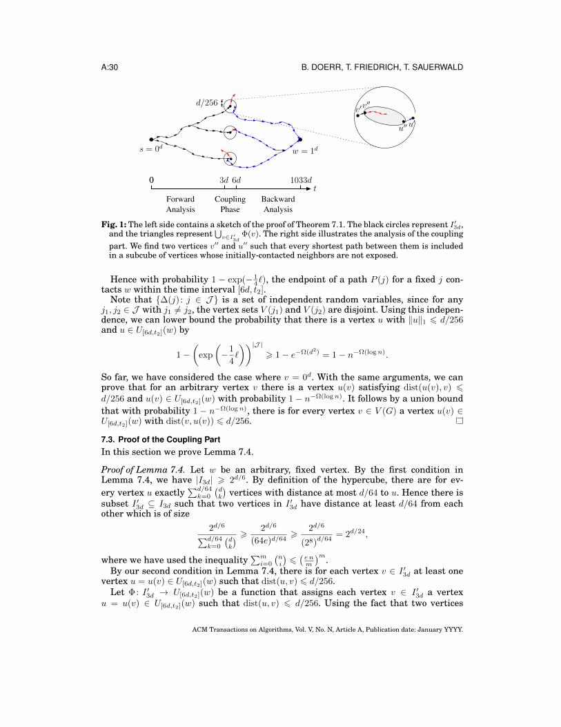
A:30 B. DOERR, T. FRIEDRICH, T. SAUERWALD
Coupling
Analysis Phase
Forward
Analysis
Backward
t0
s = 0d
v′
u′′ u′
1033d6d3d
w = 1d
v′′d/256
Fig. 1: The left side contains a sketch of the proof of Theorem 7.1. The black circles represent I ′3d,and the triangles represent
⋃v∈I′
3dΦ(v). The right side illustrates the analysis of the coupling
part. We find two vertices v′′ and u′′ such that every shortest path between them is includedin a subcube of vertices whose initially-contacted neighbors are not exposed.
Hence with probability 1 − exp(− 14`), the endpoint of a path P (j) for a fixed j con-
tacts w within the time interval [6d, t2].Note that ∆(j) : j ∈ J is a set of independent random variables, since for any
j1, j2 ∈ J with j1 6= j2, the vertex sets V (j1) and V (j2) are disjoint. Using this indepen-dence, we can lower bound the probability that there is a vertex u with ‖u‖1 6 d/256and u ∈ U[6d,t2](w) by
1−(
exp
(−1
4`
))|J |> 1− e−Ω(d2) = 1− n−Ω(logn).
So far, we have considered the case where v = 0d. With the same arguments, we canprove that for an arbitrary vertex v there is a vertex u(v) satisfying dist(u(v), v) 6d/256 and u(v) ∈ U[6d,t2](w) with probability 1 − n−Ω(logn). It follows by a union boundthat with probability 1 − n−Ω(logn), there is for every vertex v ∈ V (G) a vertex u(v) ∈U[6d,t2](w) with dist(v, u(v)) 6 d/256.
7.3. Proof of the Coupling PartIn this section we prove Lemma 7.4.
Proof of Lemma 7.4. Let w be an arbitrary, fixed vertex. By the first condition inLemma 7.4, we have |I3d| > 2d/6. By definition of the hypercube, there are for ev-ery vertex u exactly
∑d/64k=0
(dk
)vertices with distance at most d/64 to u. Hence there is
subset I ′3d ⊆ I3d such that two vertices in I ′3d have distance at least d/64 from eachother which is of size
2d/6∑d/64k=0
(dk
) >2d/6
(64e)d/64>
2d/6
(28)d/64
= 2d/24,
where we have used the inequality∑mi=0
(ni
)6(e nm
)m.By our second condition in Lemma 7.4, there is for each vertex v ∈ I ′3d at least one
vertex u = u(v) ∈ U[6d,t2](w) such that dist(u, v) 6 d/256.Let Φ: I ′3d → U[6d,t2](w) be a function that assigns each vertex v ∈ I ′3d a vertex
u = u(v) ∈ U[6d,t2](w) such that dist(u, v) 6 d/256. Using the fact that two vertices
ACM Transactions on Algorithms, Vol. V, No. N, Article A, Publication date: January YYYY.
Quasirandom Rumor Spreading A:31
in I ′3d have distance at least d/64 from each other, we observe that Φ is an injectivefunction.
Let us now fix a pair of vertices v ∈ I ′3d and Φ(v) ∈ U[6d,t2](w). Note that the set of allshortest paths between v and Φ(v) form a subcube H ′ = H ′(v,Φ(v)) whose dimensionis equal to the distance between v and Φ(v). Now choose a pair of vertices v′ ∈ H ′ ∩ I3dand u′ ∈ H ′ ∩ U[6d,t2](w) such that dist(v′, u′) is minimized. Our aim is to lower boundthe probability that v′ reaches u′ within the time interval [3d, 6d].
First let us assume that dist(v′, u′) 6 3. In this case, u′ is informed within 3d stepswith probability 1. Otherwise, we have dist(v′, u′) > 4. In this case, let v′′ ∈ Γ(v′) andu′′ ∈ Γ(u′) be two vertices such that dist(v′′, u′′) = dist(v′, u′)− 2. Note that v′′ ∈ I4d andu′′ ∈ U[5d,t2](w). By our construction, every vertex on a shortest path between v′′ andu′′ (except u′′) has distance at least one to I3d and distance at least two to U[6d,t2](w).Hence for each vertex on such a shortest path, the initially-contacted neighbor is stillchosen uniformly at random and independently of all other vertices.
Similarly to the proof of Lemma 7.3, we lower bound the probability that there existsa path P = P (v) = (v1 = v′′, v2, . . . , vdist(v′′,u′′) = u′′) which satisfies the following twoconditions for any 1 6 i < dist(v′′, u′′):
— vi+1 is closer to u′′ than vi and— vi informs vi+1 at step 4d+ i.
Note that once the rumor has reached a vertex vi for the first time, the vertex vi for-wards it to a vertex vi+1 closer to v′′ with probability at least (dist(v′′, u′′) − i + 1)/d.Repeating this argument gives the following lower bound for the existence of P :
d/256∏i=1
i
d=
(d/256)!
dd/256>
dd/256
(768 d)d/256>(2−10
)d/256> 2−d/25,
where we have used the fact that n! > (n/3)n for any integer n in the left inequality.Our next claim is that P (v) exists : v ∈ I ′3d is a set of mutually independent events.
In order to prove this, let us consider two arbitrary vertices v1, v2 ∈ I ′3d, v1 6= v2.Recall that by definition of I ′3d, dist(v1, v2) > d/64. Since every vertex on a shortestpath between vi and Φ(vi) has a distance of at most d/256 to vi, it holds by the triangleinequality that the two paths P (v1) and P (v2) always have a distance of at least d/128from each other, which proves the claimed independence.
Using this, we can lower bound the probability that at least one P (v) exists by
1−(
1− 2−d/25)2d/24
> 1− exp(−2d/(24·25)
)= 1− exp (−poly(n)) .
If there is a v ∈ I ′3d for which P (v) exists, then we know that there is a vertex v′′(v) ∈ I ′4dwhich reaches a vertex u′′(v) ∈ U[5d,t2](w) within the time interval [3d, 6d]. This impliesthat u(v) ∈ U[6d,t2](w) is informed at step 6d, and as a consequence, w will becomeinformed at step t2.
7.4. Failure ProbabilityWe now examine the probabilities in the runtime bounds for the hypercube moreclosely. Recall that the runtime bound of O(log n) for the quasirandom model holdswith probability at least 1−n−Ω(logn). In the fully random model, however, a fixed ver-tex remains uninformed for x steps with probability at least (1 − 1/d)dx > 4−x. Hencethe runtime of the fully random model is at least ρ · log2 n with probability at least n−2ρ
for any value of ρ > 1. Hence if ρ = (c/2) log2 n for some constant c > 0, this shows thatthe time for the fully random model to inform all n vertices with probability at least
ACM Transactions on Algorithms, Vol. V, No. N, Article A, Publication date: January YYYY.
A:32 B. DOERR, T. FRIEDRICH, T. SAUERWALD
1 − n−c log2 n is at least (c/2)(log2 n)2 = Ω(log(n)2). This should be compared with ourupper bound of O(log n) for the quasirandom model, which holds with probability atleast 1− n−Ω(logn).
8. CONCLUSION AND OUTLOOKIn this paper, we proposed and investigated a quasirandom analogue of the classicalpush model for spreading a rumor to all vertices of a network.
We showed that for many network topologies, after Θ(log n) iterations all verticesare informed with probability 1 − O(poly(n)). Hence the quasirandom model achievesasymptotically the same bounds as the random one, or even better ones (e. g. for ran-dom graphs with p close to log(n)/n).
This work is also interesting from the methodological point of view. Our proofs show,in particular, that the difficulties usually invoked by highly dependent random exper-iments can be overcome. From the general perspective of using randomized methodsin computer science, our results, as a number of other recent results, can be viewedas suggesting that choosing the right dose of randomness might be a fruitful topic forfurther research.
An interesting open problem is to analyze the quasirandom push model on othergraph classes. A natural candidate would be the class of regular graphs with constantconductance, for which it is known that the classical push model spreads a rumor inO(log n) rounds [Giakkoupis 2011; Chierichetti et al. 2010a]. Another interesting tar-get are preferential attachment graphs. Here [Doerr et al. 2011a] have shown that thefully random push-pull model has a broadcast time of Θ(log n), whereas the variantwith contactees chosen uniformly at random from all neighbors except the previouscontactee has a broadcast time of only Θ(log n/ log log n). Since the quasirandom pro-tocol automatically avoids the previous contactee, it seems likely that it also has thissuperior broadcast time.
Note however that it is not true that the quasirandom model always performs atleast as good as the fully random model. For instance, consider the graph consisting oftwo cliques of size n/2 − 1 and an extra vertex which is connected to all other n/2 − 2vertices. On this graph the fully random model spreads a rumor inO(log n) rounds withhigh probability, whereas the quasirandom model needs Ω(n) rounds with probabilityat least 1/4 for appropriately chosen lists.
ReferencesANGELOPOULOS, S., DOERR, B., HUBER, A., AND PANAGIOTOU, K. 2009. Tight bounds for quasirandom
rumor spreading. The Electronic Journal of Combinatorics 16, #R102.BARABASI, A.-L. AND ALBERT, R. 1999. Emergence of scaling in random networks. Science 286, 509–512.BARVE, R. D., GROVE, E. F., AND VITTER, J. S. 1997. Simple randomized mergesort on parallel disks.
Parallel Computing 23, 4-5, 601–631.BAUMANN, H., FRAIGNIAUD, P., HARUTYUNYAN, H., AND DE VERCLOS, R. 2012. The worst case behavior
of randomized gossip. In 9th Annual Conference on Theory and Applications of Models of Computation(TAMC). 330–345.
BERENBRINK, P., ELSASSER, R., AND SAUERWALD, T. 2010. Communication complexity of quasirandomrumor spreading. In 18th European Symposium on Algorithms (ESA). 134–145.
BOLLOBAS, B., RIORDAN, O., SPENCER, J., AND TUSNADY, G. 2001. The degree sequence of a scale-freerandom graph process. Random Structures & Algorithms 18, 279–290.
BOYD, S., GHOSH, A., PRABHAKAR, B., AND SHAH, D. 2006. Randomized gossip algorithms. IEEE Trans-actions on Information Theory and IEEE/ACM Transactions on Networking 52, 2508–2530.
BRODER, A. Z., FRIEZE, A. M., SHAMIR, E., AND UPFAL, E. 1994. Near-perfect token distribution. RandomStructures and Algorithms 5, 4, 559–572.
BRODER, A. Z., FRIEZE, A. M., SUEN, S., AND UPFAL, E. 1998. Optimal construction of edge-disjoint pathsin random graphs. SIAM Journal on Computing 28, 2, 541–573.
ACM Transactions on Algorithms, Vol. V, No. N, Article A, Publication date: January YYYY.
Quasirandom Rumor Spreading A:33
CHIERICHETTI, F., LATTANZI, S., AND PANCONESI, A. 2010a. Almost tight bounds for rumour spreadingwith conductance. In 42nd ACM Symposium on Theory of Computing (STOC). 399–408.
CHIERICHETTI, F., LATTANZI, S., AND PANCONESI, A. 2010b. Rumour spreading and graph conductance.In 21st ACM-SIAM Symposium on Discrete Algorithms (SODA). 1657–1663.
CHIERICHETTI, F., LATTANZI, S., AND PANCONESI, A. 2011. Rumor spreading in social networks. Theoret-ical Computer Science 412, 2602–2610.
CHUNG, F. AND LU, L. 2002. Connected components in random graphs with given expected degree se-quences. Annals of Combinatorics 6, 2, 125–145.
COOPER, C., DYER, M., AND GREENHILL, C. 2007a. Sampling regular graphs and a peer-to-peer network.Combinatorics, Probability & Computing 16, 4, 557–593.
COOPER, C., ELSASSER, R., ONO, H., AND RADZIK, T. 2012. Coalescing random walks and voting on graphs.In 31st ACM Symposium on Principles of Distributed Computing (PODC). 47–56.
COOPER, C. AND FRIEZE, A. M. 2007. The cover time of sparse random graphs. Random Structures andAlgorithms 30, 1-2, 1–16.
COOPER, J., DOERR, B., FRIEDRICH, T., AND SPENCER, J. 2010. Deterministic random walks on regulartrees. Random Structures and Algorithms 37, 3, 353–366.
COOPER, J., DOERR, B., SPENCER, J., AND TARDOS, G. 2007b. Deterministic random walks on the integers.European Journal of Combinatorics 28, 8, 2072–2090.
COOPER, J. AND SPENCER, J. 2006. Simulating a random walk with constant error. Comb. Probab. Com-put. 15, 815–822.
DEMERS, A. J., GREENE, D. H., HAUSER, C., IRISH, W., LARSON, J., SHENKER, S., STURGIS, H. E.,SWINEHART, D. C., AND TERRY, D. B. 1988. Epidemic algorithms for replicated database maintenance.Operating Systems Review 22, 1, 8–32.
DOERR, B. AND FOUZ, M. 2011. Quasi-random rumor spreading: Reducing randomness can be costly. Infor-mation Processing Letters 111, 5, 227–230.
DOERR, B., FOUZ, M., AND FRIEDRICH, T. 2011a. Social networks spread rumors in sublogarithmic time.In 43rd ACM Symposium on Theory of Computing (STOC). 21–30.
DOERR, B. AND FRIEDRICH, T. 2009. Deterministic random walks on the two-dimensional grid. Combina-torics, Probability and Computing 18, 123–144.
DOERR, B., FRIEDRICH, T., KUNNEMANN, M., AND SAUERWALD, T. 2011b. Quasirandom rumor spreading:An experimental analysis. Journal of Experimental Algorithmics 16, Article 3.3.
DOERR, B., FRIEDRICH, T., AND SAUERWALD, T. 2008. Quasirandom rumor spreading. In 19th AnnualACM-SIAM Symposium on Discrete Algorithms (SODA). 773–781.
DOERR, B., FRIEDRICH, T., AND SAUERWALD, T. 2009. Quasirandom rumor spreading: Expanders, pushvs. pull, and robustness. In 36th International Colloquium on Automata, Languages and Programming(ICALP). 366–377.
DOERR, B., HUBER, A., AND LEVAVI, A. 2013. Strong robustness of randomized rumor spreading protocols.Discrete Applied Mathematics 161, 6, 778–793.
DUBHASHI, D. AND PANCONESI, A. 2009. Concentration of Measure for the Analysis of Randomized Algo-rithms. Cambridge University Press.
DUMITRIU, I., TETALI, P., AND WINKLER, P. 2003. On playing golf with two balls. SIAM Journal on DiscreteMathematics 16, 4, 604–615.
ELSASSER, R. AND SAUERWALD, T. 2009. On the runtime and robustness of randomized broadcasting.Theoretical Computer Science 410, 36, 3414–3427.
FEIGE, U., PELEG, D., RAGHAVAN, P., AND UPFAL, E. 1990. Randomized broadcast in networks. RandomStructures and Algorithms 1, 4, 447–460.
FOUNTOULAKIS, N. AND HUBER, A. 2009. Quasirandom rumour spreading on the complete graph is as fastas randomized rumour spreading. SIAM Journal on Discrete Mathematics 23, 4, 1964–1991.
FOUNTOULAKIS, N., HUBER, A., AND PANAGIOTOU, K. 2010. Reliable broadcasting in random networksand the effect of density. In 29th IEEE International Conference on Computer Communications (INFO-COM). 2552–2560.
FOUNTOULAKIS, N. AND PANAGIOTOU, K. 2010. Rumor spreading on random regular graphs and ex-panders. In 14th International Workshop on Randomization and Computation (RANDOM). 560–573.
FOUNTOULAKIS, N., PANAGIOTOU, K., AND SAUERWALD, T. 2012. Ultra-fast rumor spreading in socialnetworks. In 23rd Annual ACM-SIAM Symposium on Discrete Algorithms (SODA). 1642–1660.
FRIEDRICH, T., GAIRING, M., AND SAUERWALD, T. 2010. Quasirandom load balancing. In 21st AnnualACM-SIAM Symposium on Discrete Algorithms (SODA). 1620–1629.
ACM Transactions on Algorithms, Vol. V, No. N, Article A, Publication date: January YYYY.
A:34 B. DOERR, T. FRIEDRICH, T. SAUERWALD
FRIEDRICH, T. AND SAUERWALD, T. 2010. The cover time of deterministic random walks. The ElectronicJournal of Combinatorics 17, 1, 1–7. R167.
FRIEZE, A. M. AND GRIMMETT, G. R. 1985. The shortest-path problem for graphs with random arc-lengths.Discrete Applied Mathematics 10, 57–77.
GIAKKOUPIS, G. 2011. Tight bounds for rumor spreading in graphs of a given conductance. In 28th Interna-tional Symposium on Theoretical Aspects of Computer Science (STACS). 57–68.
GIAKKOUPIS, G., SAUERWALD, T., SUN, H., AND WOELFEL, P. 2012. Low randomness rumor spreadingvia hashing. In 29th International Symposium on Theoretical Aspects of Computer Science (STACS).314–325.
GIAKKOUPIS, G. AND WOELFEL, P. 2011. On the randomness requirements of rumor spreading. In 22ndAnnual ACM-SIAM Symposium on Discrete Algorithms (SODA). 449–461.
HEDETNIEMI, S. M., HEDETNIEMI, S. T., AND LIESTMAN, A. L. 1988. A survey of gossiping and broadcast-ing in communication networks. Networks 18, 4, 319–349.
HOORY, S., LINIAL, N., AND WIGDERSON, A. 2006. Expander graphs and their applications. Bulletin of theAmerican Mathematical Society 43, 439–561.
KAHALE, N. 1995. Eigenvalue and expansion of regular graphs. Journal of the ACM 42, 5, 1091–1106.KARP, R., SCHINDELHAUER, C., SHENKER, S., AND VOCKING, B. 2000. Randomized rumor spreading. In
41st IEEE Symposium on Foundations of Computer Science (FOCS). 565–574.KEMPE, D., DOBRA, A., AND GEHRKE, J. 2003. Gossip-based computation of aggregate information. In 44th
IEEE Symposium on Foundations of Computer Science (FOCS). 482–491.KLEBER, M. 2005. Goldbug variations. The Mathematical Intelligencer 27, 55–63.MAHLMANN, P. AND SCHINDELHAUER, C. 2006. Distributed random digraph transformations for peer-to-
peer networks. In 18th ACM Symposium on Parallel Algorithms and Architectures (SPAA). 308–317.MCDIARMID, C. 1989. On the method of bounded differences. In Surveys in combinatorics, 1989 (Norwich,
1989). London Math. Soc. Lecture Note Ser. Series, vol. 141. Cambridge Univ. Press, Cambridge, 148–188.
MITZENMACHER, M. AND UPFAL, E. 2005. Probability and Computing: Randomized Algorithms and Prob-abilistic Analysis. Cambridge University Press.
MOSK-AOYAMA, D. AND SHAH, D. 2006. Computing separable functions via gossip. In 25th ACM-SIGOPTPrinciples of Distributed Computing (PODC). 113–122.
NIEDERREITER, H. 1992. Random number generation and quasi-Monte Carlo methods. SIAM, Philadelphia,PA, USA.
PITTEL, B. 1987. On spreading a rumor. SIAM Journal on Applied Mathematics 47, 1, 213–223.PRIEZZHEV, V. B., DHAR, D., DHAR, A., AND KRISHNAMURTHY, S. 1996. Eulerian walkers as a model of
self-organized criticality. Physical Review Letters 77, 5079–5082.RABANI, Y., SINCLAIR, A., AND WANKA, R. 1998. Local divergence of markov chains and the analysis of
iterative load balancing. In 39th IEEE Symposium on Foundations of Computer Science (FOCS). 694–705.
SAUERWALD, T. 2010. On mixing and edge expansion properties in randomized broadcasting. Algorith-mica 56, 1, 51–88.
TANNER, R. M. 1984. Explicit concentrators from generalized N -gons. SIAM Journal Algebraic DiscreteMethods 5, 3, 287–293.
WAGNER, I. A., LINDENBAUM, M., AND BRUCKSTEIN, A. M. 1996. Smell as a computational resource –a lesson we can learn from the ant. In 4th Israel Symposium on Theory of Computing and Systems(ISTCS). 219–230.
WAGNER, I. A., LINDENBAUM, M., AND BRUCKSTEIN, A. M. 1999. Distributed covering by ant-robots usingevaporating traces. IEEE Transactions on Robotics and Automation 15, 5, 918–933.
ACM Transactions on Algorithms, Vol. V, No. N, Article A, Publication date: January YYYY.
Quasirandom Rumor Spreading A:35
A. PROBABILISTIC TAIL BOUNDS USED FOR OUR ANALYSISAs our analysis heavily relies on probabilistic tails bounds, we summarize them herefor reference. The following bound can be found, e.g., in the textbook of Mitzenmacherand Upfal [2005].
LEMMA A.1 (CHERNOFF BOUNDS FOR SUMS OF BERNOULLI VARIABLES). LetXi, 1 6 i 6 n, be independent random variables. Let X =
∑ni=1Xi, 0 < p < 1 and δ > 0.
If Pr [Xi = 1] = p and Pr [Xi = 0] = 1− p for all i ∈ 1, . . . , n, then
Pr [X 6 (1− δ)E [X]] 6 exp(−δ2 E [X] /2
),
Pr [X > (1 + δ)E [X]] 6 exp(−minδ, δ2E [X] /3
).
We also use the following concentration bound, which is also called the method ofbounded differences [McDiarmid 1989, Lemma 1.2].
LEMMA A.2 (AZUMA’S INEQUALITY). Let Xi : Ωi → R, 1 6 i 6 n, be mutually inde-pendent random variables. Let f :
∏ni=1 Ωi → R satisfy the Lipschitz condition
|f(x)− f(x′)| 6 ci
where x and x′ differ only in the i-th coordinate, 1 6 i 6 n. Let Y be the random variablef(X1, . . . , Xn). Then for any t > 0,
Pr [Y > E [Y ] + t] 6 exp(−2t2/∑ni=1 c
2i ).
We shall also use the concept of stochastic domination between random variables.
Definition A.1. A random variable X is stochastically smaller than Y , if for allk ∈ R, Pr [X > k] 6 Pr [Y > k]. In this case, we also write X Y .
We list two obvious facts about stochastic domination.
LEMMA A.3. Let X1, X2 be two independent random variables and let Y1, Y2 be twoadditional independent random variables with X1 Y1 and X2 Y2. Then,
—X1 +X2 Y1 + Y2 and— minX1, X2 minY1, Y2.
We continue with a simple fact about the geometric distribution.
LEMMA A.4. Let X1, X2, . . . , Xn be n independent geometric random variables eachwith parameter 0 < p < 1. Then X := minni=1Xi is a geometric random variable withparameter (1− (1− p)n).
We use the following standard Chernoff bound for sums of geometric random vari-ables from [Dubhashi and Panconesi 2009, Problem 3.6].
LEMMA A.5 (CHERNOFF BOUND FOR SUMS OF GEOMETRIC VARIABLES). LetY1, Y2, . . . , Yn be independent geometric random variables, each with parameter p > 0.Let Y :=
∑ni=1 Yi. Then for any ε > 0,
Pr
[Y > (1 + ε)
n
p
]6 exp
(− ε2
2 (1 + ε)n
).
ACM Transactions on Algorithms, Vol. V, No. N, Article A, Publication date: January YYYY.

![EIGENVALUES AND LINEAR QUASIRANDOM HYPERGRAPHS · Eigenvalues and linear quasirandom hypergraphs 3 Disc: For every U V.Hn/, jE.HnTUU/jDp jUj k Co.nk/. Count[linear]: For every fixed](https://img.pdfslide.us/doc/110x75/5f680c88de314b0f57018a9c/eigenvalues-and-linear-quasirandom-hypergraphs-eigenvalues-and-linear-quasirandom.jpg)