MAX-PLANCK-INSTITUT ••

FUR INFORMATIK

Sequential and parallel algori thms for

the k closest pairs problem

Hans-Peter Lenhof Mi chi el Smid

MPI-I-92-134 August 1992

o

mPD _________ I N F 0 R M AT I K _________ _

Im Stadtwald

66123 Saarbrücken

Germany

Sequential and parallel algorithms for

the k closest pairs problem

Hans-Peter Lenhof Michiel Smid

MPI-I-92-134 August 1992

Sequential and parallel algorithms for the k closest pairs problem*

Hans-Peter Lenhoft Michlel Smid t Max-Planck-Institut für Informatik

W-6600 Saarbrücken, Germany

August 7, 1992

Abstract

Let S be a set of n points in D-dimensional space, where D is a constant, and let k be an integer between 1 and (~). A new and simpler proof is given of Salowe's theorem, i.e., a sequential algorithmis given that computes the k c10sest pairs in the set S in O(nlogn + k) time, using O(n + k) space. The algorithm fits in the algebraic decision tree model and is, therefore, optimal. Salowe's algorithm seems difficult to parallelize. A parallel version of our algorithm is given for the CRCW-PRAM model. This version runs in O((logn)2Ioglogn) expected parallel time and has an 0 ( n log n log log n+ k) time-processor product.

1 Introduction

There has been a lot of interest in closest pair problems. In such problems, we are given a set of n points in D-dimensional space, and we want to compute the closest pair, all k closest pairs, or just the k-th closest pair. Distances are measured in an arbitrary Lt-metric, where 1 :::; t :::; 00. In this metric, the distance dt(p, q) between the points P = (PI, ... ,PD) and q = (ql' ... , qD) is defined by

if 1 :::; t < 00, and for t = 00, it is defined by

• A preliminary version of this paper will appear in the Proceedings of the 33-rd Annual IEEE Symposium on Foundations of Computer Science, 1992, under the title Enumerating the k closest pairs optimally.

tThis work was supported by the ESPRIT Basic Research Actions Program, under contract No. 7141 (project ALCOM 11).

1

The problem of finding the closest pair has been solved already for a long time. Shamos and Hoey [13J and BentIey and Shamos [2J solve this problem, for the case D = 2 and D 2: 2, respectively, in O(nlog n) time, which is optimal in the algebraic decision tree model. RecentIy, an optimal algorithm for the on-line version of this problem has been given by Schwarz et al. [12J.

For the problem of computing the k-th closest pair, there are results by Agarwal et al. [1], who consider the Lt-metric for the planar case, and by Salowe [10J, who shows how to select the k-th closest pair in the Loo-metric in O(n(log n)D) time, for any fixed D 2: 2.

For the problem of enumerating the k closest pairs, the first result was by Smid [14], who shows how to compute the n 2

/3 closest pairs in a set of n points in D-space in

O(nlog n) time. This result was extended in two directions. First, for the planar case, Dickerson and Drysdale [5] compute the k closest pairs-ordered by their distances-in O(nlog n+k log n) time. Second, Salowe [l1J gives an optimal algorithm that computes the k closest pairs in O( n log n + k) time. The latter result holds for an arbitrary, but fixed, dimension D. Salowe's algorithm uses complicated techniques such as parametric search and Vaidya's algorithm for the all-nearest-neighbors problem, see [15].

Katoh and Iwano [7J give a technique for solving related problems such as finding the k furthest pairsor the k closest/furthest bichromatic pairs. Their technique can also be applied to the k closest pairs problem. The result is an algorithm with running time O(nlogn+ klognlog(n2 /k)). (See [8].)

In this paper, we give a new proof of Salowe's theorem: We show how to compute the k closest pairs in O( n log n + k) time. The algorithm works for any t, 1 ::; t ::; 00,

any fixed dimension D and any k, 1 < k ::; (;). The algorithm fits in the algebraic decision tree model and is, therefore, optimal. (The constant factor is of the form ~logD, for some c.) We remark that our algorithm does not enumerate the k closest pairs in sorted order; the order can bearbitrary.

Comparing our technique with that of Salowe, our approach has the advantage that it is completely self-contained. Moreover, as we will see, our version can be parallelized, whereas this seems to be diflicult for Salowe's algorithm.

Our algorithm is based on the fact that once the k-th smallest Lt-distance die is known, we can easily enumerate the k closest pairs: Consider a grid with cells of length die and distribute the points over the cells. Then, compare each point with all points that are contained in one of the 3D neighboring cells. Of course, this algorithm takes too many pairs in consideration. All pairs that are looked at, however, have Lt-distance at most 2Ddle • (Equality can occur in the L1-metric.) By a result of Salowe [l1J, see Lemma 2, the number of pairs considered is O(k + n). Therefore, we find the k closest pairs in O( n log n + k) time.

Of course, the k-th smallest Lt-distance is not known at the start of the algorithm. We could approximate it by running Salowe's algorithm that finds the k-th smallest Loo-distance. This takes, however, O(n(1og n)D) time. As we shall see, for our appli­cation, it suffices to approximate the k-th Loo-distance. Such an approximation can be found in O( n log n) time. .

. We also give a parallel version of our algorithm. As mentioned already, Salowe's algorithm seems diflicult to parallelize. Our parallel version uses the CRCW-PRAM

2

model. It has an expected running time of O( (log n? log log n) and uses n /log n + k / ((log n )2 log log n) processors. That is, the product of the time complexity and the number ofprocessors is O(nlognloglogn + k).

We have not found any results in the literature about the parallel complexity of the k closest pairs problem, except for the case k = 1. Cole and Goodrich [4] have shown that in the plan ar case, the closest pair in a set of n points can be found deterministically in O(log n) time using n processors. They obtain this result for the EREW-PRAM model. As far as we know, there are no non-trivial results for the closest pair problem in higher dimensions. Our algorithm finds the closest pair in a set of n points in D-space in O( (log n? log log n) expected time using n / log n processors. Therefore, for D > 2, this is the best result known at this moment.

The rest of this paper is organized as follows . In Section 2, we prove some combi­natorial results that are needed in the analysis of the algorithm. In Section 3, we give the sequential algorithm, which consists of two phases. First, in Subsection 3.1, we compute an Loo-distance with rank 9(k + n). (Here, the term n appears because of a technical reason that will become clear later.) The algorithm implicitly manipulates all possible differences Ipi - qil, where 1 ~ i ~ D and P and q are points of the input set. It makes a binary search on these differences. (The way in which the binary search is controlled is due to Johnson and Mizoguchi [6], who use it to find the k-th smallest element in the Cartesian sum X + Y.) After a presorting step, which takes O(nlog n) time, we can test in O(n) time, if a difference Ipi - qil approximates the desired L oo -

distance. The approximation is found within O(log n) iterations. In Subsection 3.2, this approximation is used to find the k closest pairs w.r.t. the Lt-metric. Of course, we can use the above sketched algorithm that uses a grid. Then, however, in order to distribute the points over the cells, we need the non-algebraic Hoor-function. Instead, we use a slightly degenerate grid that can be constructed without the Hoor-function.

In Section 4, we give a parallel implementation of our algorithm. We express the complexity of a parallel algorithm by giving the time bound f( n) and the amount of work g(n). This means that the algorithm takes O(f(n)) parallel time using g(n)/ f(n) processors. We finish the paper in Section 5 with some open problems.

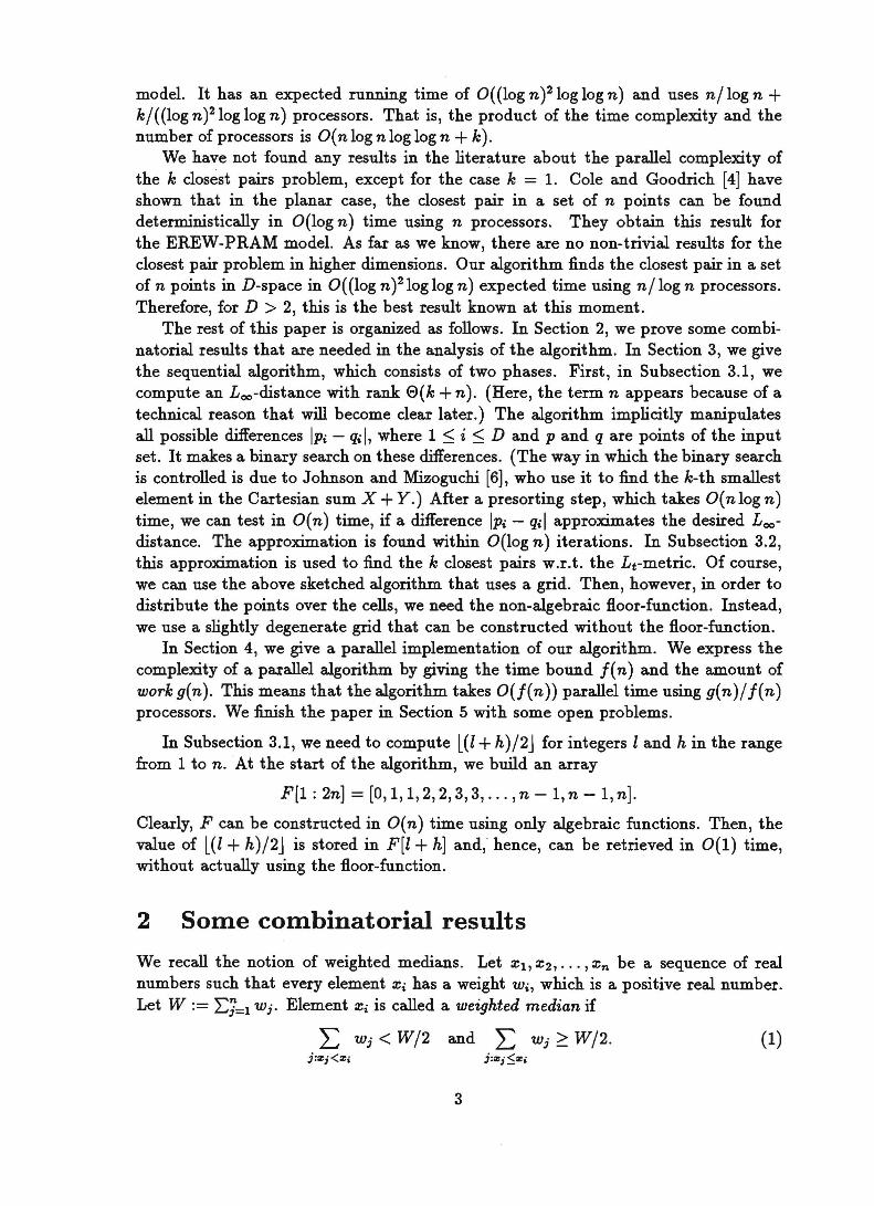
In Subsection 3.1, we need to compute l(l + h)/2 J for integers land hin the range !rom 1 to n. At the start of the algorithm, we build an array

F[l : 2n] = [0,1,1,2,2,3,3, . . . ,n - 1, n - 1, n].

Clearly, F can be constructed in O(n) time using only algebraic functions . Then, the value of l(l + h)/2 J is stored in F[l + h] and, hence, can be retrieved in 0(1) time, without actually using the Hoor-function.

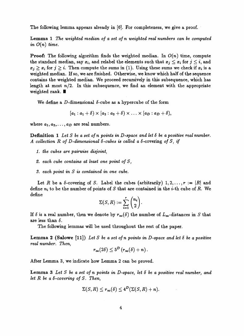
2 Some combinatorial results

We recall the notion of weighted medians. Let :1::1, :1::2, ••• ,:l::n be a sequence of real numbers such that everyelement :l::i has a weight Wi, which is a positive real number. Let W := Ei=l Wj. Element :l::i is called a weighted median if

L Wj < W/2 and L Wj ~ W/2. (1)

3

The following lemma appears already in [6]. For completeness, we give a proof.

Lemma 1 The weighted median 0/ a set 0/ n weighted real numbers can be computed in O( n) time.

Proof: The following algorithm finds the weighted median. In O( n) time, compute the standard median, say Zi, and relabel the elements such that Zj < Zi for j ~ i, and Zj ~ Zi for j ~ i. Then compute the sums in (1). Using these sums we check if Zi is a weighted median. If so, we are finished. Otherwise, we know which half of the sequence contams the weighted median. We proceed recursively in this subsequence, which has length at most n/2. In this subsequence, we find an element with the appropriate weighted rank .•

We define a D-dimensional 8-cube as a hypercube of the form

[al: al + 8) x [a2 : a2 + 8) x ... X raD : aD + 8),

where al, a2J. . .. , aD are real numbers.

Definition 1 Let S be a set 0/ n points in D-space and let 8 be a positive real number. A collection R 0/ D-dimensional 8-cubes is called a 8-covering 0/ S, i/

1. the cubes are pairwise dis joint,

2. each cube contains at least one point 0/ s,

3. each point in S is contained in one cube.

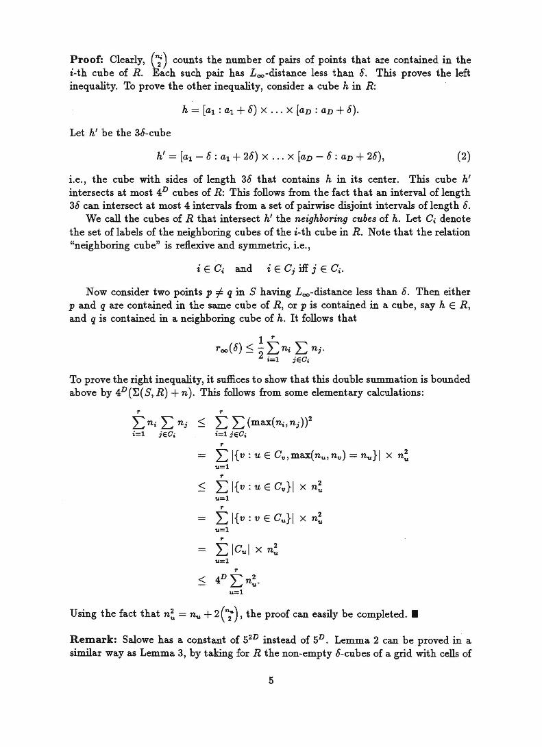
Let R be a 8-covering of S. Label the cubes (arbitrarily) 1,2, ... ,r:= IRI and define ni to be the number of points of S that are contained in the i-th cube of R. We define

,. (ni) ~(S, R) := L: . i=l 2

If 8 is areal number, then we denote by roo (8) the number of Loo-distances in S that are less than 8.

The following lemmas will be used throughout the rest of the paper.

Lemma 2 (Salowe [11]) Let S be a set o/n points in D-space and let 8 be a positive real number. Then,

roo (28) ~ SD (roo ( 8) + n) .

After Lemma 3, we indicate how Lemma 2 can be proved.

Lemma 3 Let S be a set 0/ n points in D-space, let 8 be a positive real number, and let R be a 8-covering 0/ S. Then,

~(S, R) ~ r6c(8) ~ 4D(~(S, R) + n).

4

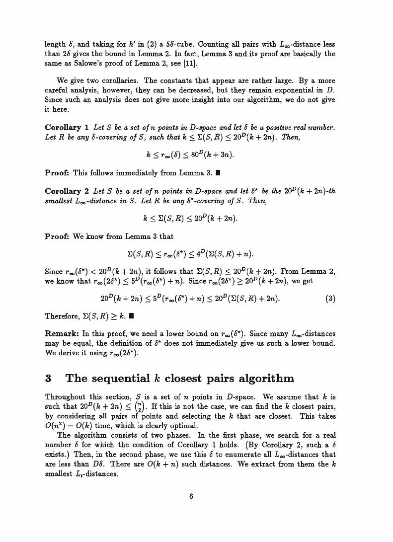
Proof: Clearly, (~) counts the number of pairs of points that are contained in the i-th cube of R. Each such pair has Loo-distance less than 8. This proves the left inequality. To prove the other inequality, consider a cube h in R:

h = [al: al + 8) x ... X [aD : aD + 8).

Let h' be the 38-cube

h' = [al - 8 : al + 28) x ... X [aD - 8 : aD + 28), (2)

i.e., the cube with sides of length 38 that contains h in its center. This cube h' intersects at most 4D cubes of R: This follows hom the fact that an interval of length 38 can intersect at most 4 intervals hom a set of pairwise disjoint intervals of length 8.

We call the cubes of R that intersect h' the neighboring cubes of h. Let Ci denote the set of labels of the neighboring cubes of the i-th cube in R. Note that the relation "neighboring cube" is reflexive and symmetrie, i.e.,

i E Ci and i E C; iff j E Ci.

N ow consider two points p =1= q in S having Loo-distance less than 8. Then either p and q are contained in the same cube of R, or p is contained in a cube, say hER, and q is contained in a neighboring cube of h. It follows that

To prove the right inequality, it suffices to show that this double summation is bounded above by 4D (1::( S, R) + n). This follows hom some elementary calculations:

~ ~

L:ni L: n; < L: L: (max(ni, nj))2 i=l ;EC. i=l ;EC.

~

- L: I{v: u E C",max(nu,n,,) = nu}1 x n2 u

u=l ~

< L: I{v : U E C,,}I x n2 u

u=! ~

L: I{ v : v E Cu}1 x n2 u

u=l ~

L:ICul x n 2 u

u=l ~

< 4D L: n~. u=l

U sing the fact that n~ = nu + 2 (7) , the proof can easily be completed .•

Remark: Salowe has a constant of s2D instead of SD. Lemma 2 can be proved in a similar way as Lemma 3, by taking for R the non-empty 8-cubes of a grid with cells of

S

length 8, and taking for h' in (2) a 58-cube. Counting all pairs with Loo-distance less than 28 gives the bound in Lemma 2. In fact, Lemma 3 and its proof are basically the same as Salowe's proof of Lemma 2, see [11].

We give two corollaries. The constants that appear are rather large. By a more careful analysis, however, they can be decreased, but they remain exponential in D. Since such an analysis does not give more insight into our algorithm, we do not give it here.

CoroUary 1 Let S be a set 0/ n points in D-space and let 8 be a positive real number. Let R be any 8-covering 0/ S, such that k :::; ~(S, R) :5 20D(k + 2n). Then,

k :::; roo (8) :::; 80D (k + 3n).

Proof: This follows immediately from Lemma 3 .•

Corollary 2 Let S be a set 0/ n points in D-space and let 8* be the 20D (k + 2n )-th smallest Loo-distance in S. Let R be any 8*-covering 0/ S. Then,

k :::; ~(S, R) :::; 20D(k + 2n).

Proof: We know from Lemma 3 that

~(S, R) :::; roo (8*) :::; 4D(~(S, R) + n).

Since roo (8*) < 20D(k + 2n), it follows that ~(S, R) :::; 20D(k + 2n). From Lemma 2, we know that roo (28*) :::; 5D(roo (8*) + n). Since roo (28*) ~ 20D(k + 2n), we get

20D(k + 2n) :5 5D(roo(8*) + n) :::; 20D(~(S, R) + 2n). (3)

Therefore, ~(S, R) > k .•

Remark: In this proof, we need a lower bound on roo ( 8*). Since many Loo-distances may be equal, the definition of 8* does not immediately give us such a lower bound. We derive it using roo (28*).

3 The sequential k closest pairs algorithm

Throughout this section, S is a set of n points in D-space. We assume that k is such that 20D(k + 2n) :::; (;). If this is not the case, we can find the k closest pairs, by considering all pairs of points and selecting the k that are closest. This takes O(n2

) = O(k) time, which is clearlyoptimal. The algorithm consists of two phases. In the first phase, we search for areal

number 8 for which the condition of Corollary 1 holds. (By Corollary 2, such a 8 exists.) Then, in the second phase, we use this 8 to enumerate all Loo-distances that are less than D8. There are O(k + n) such distances. We extract from them the k smallest Lt-distances.

6

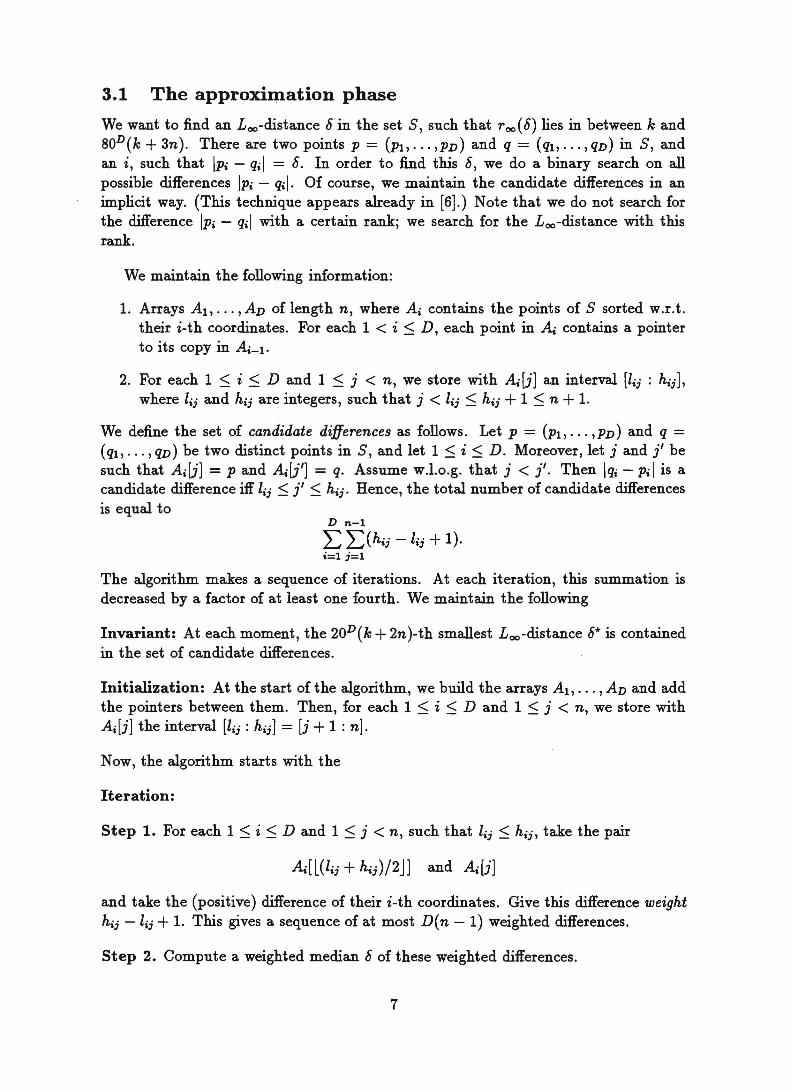
3.1 The approximation phase

We want to find an Loo-distance 8 in the set S, such that roo (8) lies in between k and 80D(k + 3n). There are two points P = (Pll ... ,PD) and q = (qb ... ,qD) in S, and an i, such that Ipi - qil = 8. In order to find this 8, we do a binary search on all possible differences Ipi - qil. Of course, we maintain the candidate differerices in an implicit way. (This technique appears already in [6].) Note that we do not search for the difference Ipi - qil with a certain rank; we search for the Loo-distance with this rank.

We maintain the following information:

1. Arrays All" ., A D of length n, where Ai contains the points of S sorted w.r.t. their i-th coordinates. For each 1 < i :s; D, each point in ~ contains apointer to its copy in ~-1'

2. For each 1 :s; i :s; D and 1 :s; j < n, we store with ~[j] an interval [lii : kii ] , where lii and k ii are integers, such that j < lii :s; k ii + 1 :s; n + 1.

We define the set of candidate diJJerences as follows. Let p = (PI,"" PD) and q = ( ql, ... , qD) be two distinct points in S, and let 1 :s; i :s; D. Moreover, let j and j' be such that Ai[j] = p and ~[j'] = q. Assume w.l.o.g. that j < j'. Then Iqi - Pil is a candidate difference iff lii :s; j' :s; k ii . Hence, the total number of candidate differences is equal to

D n-l

'E 'E(kii -lii + 1). i=1 i=1

The algorithm makes a sequence of iterations. At each iteration, this summation is decreased by a factor of at least one fourth. We maintain the following

Invariant: At each moment, the 20D (k + 2n)-th smallest Loo-distance 8* is contained in the set of candidate differences.

Initialization: At the start of the algorithm, we build the arrays Ab ... , AD and add the pointers between them. Then, for each 1 :s; i :s; D and 1 :s; j < n, we store with ~[j] the interval [lii : kii] = [j + 1 : n].

N ow, the algorithm starts with the

Iteration:

Step 1. For each 1 :s; i :s; D and 1 :s; j < n, such that lii :s; k ii , take the pair

and take the (positive) difference of their i-th coordinates. Give this difference weigkt kii - lij + 1. This gives a sequence of at most D( n - 1) weighted differences.

Step 2. Compute a weighted median 8 of these weighted differences.

7

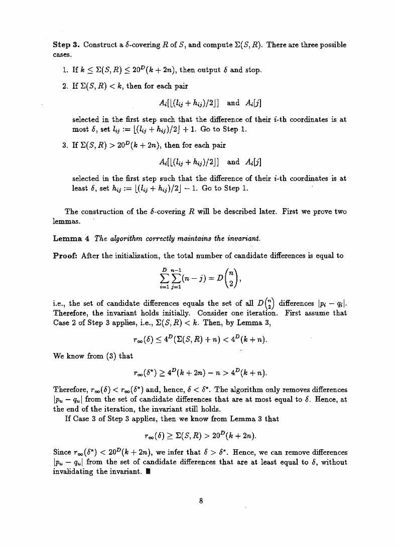
Step 3. Construct a 8-covering R of S, and compute ~(S, R). There are three possible cases.

1. If k < ~(S, R) :::; 20D (k + 2n), then output 8 and stop.

2. If ~(S, R) < k, then for each pair

~[l(lij + hij )/2J] and Ai[j]

selected in the first step such that the difference of their i-th coordinates is at most 8, set lij := l(lij + hij )/2J + 1. Go to Step 1.

3. If ~(S, R) > 20D (k + 2n), then for each pair

~[l(lij + ~j)/2J] and ~[j]

selected in the first step such that the difference of their i-th coordinates is at least 8, set hij := l(lij + hij )/2J - 1. Go to Step 1.

The construction of the 8-covering R will be described later. First we prove two lemmas.

Lemma 4: The algorithm correctly maintains the invariant.

Proof: After the initialization, the total number of candidate differences is equal to

D n-l ( ) t; ~(n - j) = D ~ ,

i.e., the set of candidate differences equals the set of all n(;) differences Ipi - qil. Therefore, the invariant holds initially. Consider one iteration. First assume that Case 2 of Step 3 applies, i.e., ~(S, R) < k. Then, by Lemma 3,

T oo (8) :::; 4D(~(S, R) + n) < 4D(k + n).

We know from (3) that

T oo (8*) ~ 4D (k + 2n) - n > 4D (k + n).

Therefore, T oo (8) < T oo (8*) and, hence, 8 < 8*. The algorithm only removes differences Ipu - qu I from the set of candidate differences that are at most equal to 8. Hence, at the end of the iteration, the invariant still holds.

If Case 3 of Step 3 applies, then we know from Lemma 3 that

T oo (8) > ~(S,R) > 20D (k + 2n).

Since T oo (8*) < 20D (k + 2n), we infer that 8 > 8*. Hence, we can remove differences Ipu - qul from the set of candidate differences that are at least equal to 8, without invalidating the invariant .•

8

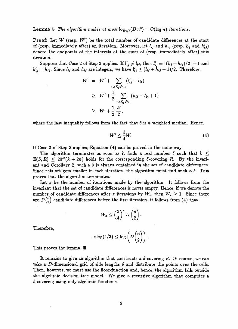
Lemma 5 The algorithm makes at most log4/3(D n 2) = O(log n) iterations.

Proof: Let W (resp. W') be the total number of candidate differences at the start of (resp. immediately after) an iteration. Moreover, let "Zij and hij (resp. l~j and h~j) denote the endpoints of the intervals at the start of (resp. immediately after) this iteration.

Suppose that Case 2 of Step 3 applies. If Z~j i- Zij, then Z~j = l(Zij + hij )/2J + 1 and h~j = hij . Since lij and hij are integers, we have Z~j ~ (lij + ~j + 1)/2. Therefore,

W = W' + L: (Z~j - Zij) i,j:Z:;#i;

where the last inequality follows from the fact that 8 is a weighted median. Hence,

W'<~W -4

If Case 3 of Step 3 applies, Equation (4) can be proved in the same way.

(4)

The algorithm terminates as soon as it finds areal number 8 such that k $ ~(S, R) $ 20D (k + 2n) holds for the corresponding 8-covering R. By the invari­ant and. Corollary 2, such a 8 is always contained in the set of candidate differences. Since this set gets smaller in each iteration, the algorithm must find such a 8. This proves that the algorithm terminates.

Let z be the number of iterations made by the algorithm. It follows from the invariant that the set of candidate differences is never empty. Hence, if we denote the number of candidate differences after z iterations by W.z:, then W.z: > 1. Since there are D (;) candidate differences before the first iteration, it follows from (4) that

Therefore,

zlog(4/3) $ log (D(;)) . This proves the lemma .•

It remains to give an algorithm that constructs a 8-covering R. Of course, we can take a D-dimensional grid of side lengths 8 and distribute the points over the cells. Then, however, we must use the fioor-function and, hence, the algorithm falls outside the algebraic decision tree model. We give a recursive algorithm that computes a 8-covering using only algebraic functions.

9

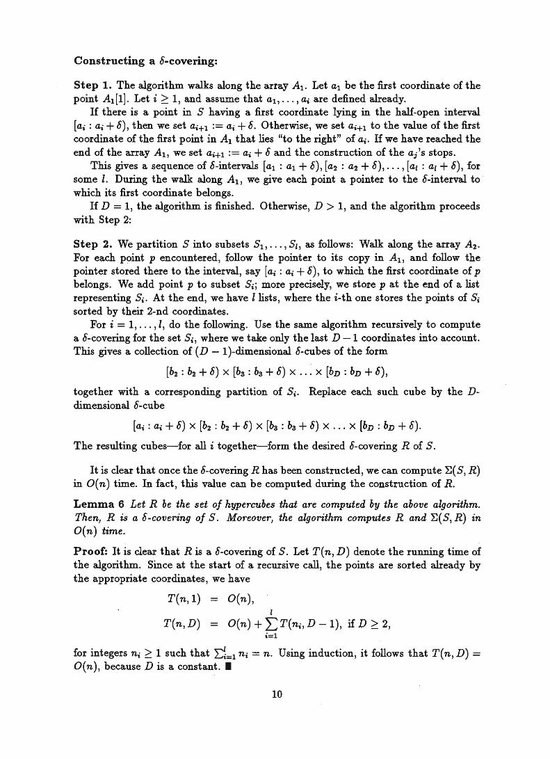
Constructing a S-covering:

Step 1. The algorithm wills along the array Al' Let a1 be the first coordinate of the point A1[1]. Let i 2:: 1, and assume that a1, . .. , ai are defined already.

If there is a point in S having a first coordinate lying in the half-open interval [ai: ai + S), then we set ai+1 := ai + S. Otherwise, we set ai+1 to the value of the first co ordinate of the first point in Al that lies "to the right" of ai. H we have reached the end of the array Al, we set ai+1 := ai + S and the construction of the a;'s stops.

This gives a sequence of S-intervals [al: a1 + S), [a2 : a2 + S), .. . , [a, : a, + S), for some 1. During the will along Al, we give each point apointer to the S-interval to which its first coordinate belongs.

If D = 1, the algorithm is finished. Otherwise, D > 1, and the algorithm proceeds with Step 2:

Step 2. We partition Sinto subsets Sl'" ., S"~ as folIows: Will along the array A2 •

For each point p encountered, follow the pointer to its copy in Al, and follow the pointer stored there to theinterval, say [ai: ai + S), to which the first coordinate of p belongs. We add point p to subset Si; more precisely, we store p at the end of a list representing Si. At the end, we have 1lists, where the i-th one stores the points of Si sorted by their 2-nd coordinates.

For i = 1, ... , I, do the following. Use the same algorithm recursively to compute a S-covering for the set Si, where we take only the last D -1 coordinates into account. This gives a collection of (D - 1 )-dimensional S-cubes of the form

[b2 : b2 + S) x [ba: ba + S) x ... X [bD : bD + S),

together with a corresponding partition of Si. Replace each such cube by the D­dimensional S-cube

[ai: ai + S) X [b2 : b2 + S) x [ba: ba + S) x ... X [bD : bD + S).

The resulting cubes-for all i together-form the desired S-covering R of S.

It is clear that once the S-covering R has been constructed, we can compute ~(S, R) in O( n) time. In fact, this value can be computed during the construction of R.

Lemma 6 Let R be the set 01 hypercubes that are computed by the above algorithm. Then, R is a S -covering 01 S. M oreover, the algorithm computes R and ~(S, R) in O(n) time.

Proof: It is clear that R is a S-covering of S. Let T(n, D) denote the running time of the algorithm. Since at the start of a recursive call, the points are sorted already by the appropriate coordinates, · we have

T(n, 1)

T(n, D)

O(n), l

O(n) + 'LT(ni' D -1), if D 2:: 2, i=l

for integers ni 2:: 1 such that ~=l ni = n. Using induction, it follows that T(n, D) = O(n), because D is a constant .•

10

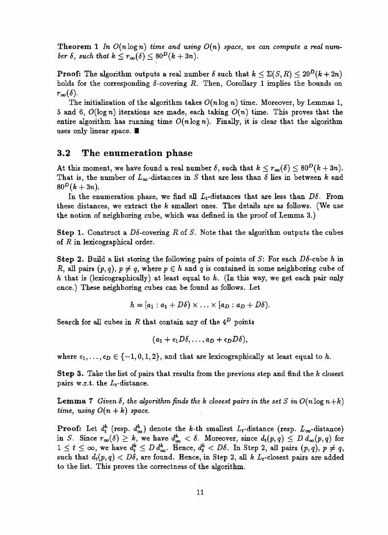
Theorem 1 In O( n log n) time and using O( n) space, we can compute areal num­ber 0, such that k ::; Too(O) ::; 80D (k + 3n).

Proof: The algorithm outputs areal number 0 such that k ::; ~(s, R) ::; 20D (k + 2n) holds for the corresponding o-covering R. Then, Corollary 1 implies the bounds on T oo ( 0).

The initialization of the algorithm takes O(nlog n) time. Moreover, by Lemmas 1, 5 and 6, O(log n) iterations are made, each taking O( n) time. This proves that the entire algorithm has running time O( n log n). Finally, it is dear that the algorithm uses only linear space. •

3.2 The enumeration phase

At this moment, we have found areal number 0, such that k ::; Too(O) ::; 80D (k + 3n). That is, the number of Loo-distances in S that are less than 0 lies in between k and 80D (k + 3n).

In the enumeration phase, we find all Lt-distances that are less than Do. From these distances, we extract the k smallest ones. The details are as follows. (We use the notion of neighboring cube, which was defined in the proof of Lemma 3.)

Step 1. Construct a Do-covering R of S. Note that the algorithm outputs the cubes of R in lexicographical order.

Step 2. Build a list storing the following pairs of points of S: For each Do-cube h in R, all pairs (p, q), p =J q, where p E hand q is contained in some neighboring cube of h that is (lexicographically) at least equal to h. (In this way, we get each pair only once.) These neighboring cubes can be found as follows. Let

h = [al: al + Do) X ... X raD : aD + DO).

Search for all cubes in R that contain any of the 4D points

where EI, .•• , ED E {-1, 0,1, 2}, and that are lexicographically at least equal to h.

Step 3. Take the list of pairs that results from the previous step and find the k dosest pairs w.r.t. the Lt-distance.

Lemma 7 Given 0, the algorithm finds the k closest paiTs in the set S in O( n log n + k ) time, using O( n + k) space.

Proof: Let d; (resp. d~) denote the k-th smallest Lt-distance (resp. Loo-distance) in S. Since Too(O) ~ k, we have d~ < o. Moreover, since dt(p, q) ::; D doo(p, q) for 1 ::; t ::; 00, we have d; ::; D d~. Hence, d; < Do. In Step 2, all pairs (p, q), p =J q, such that dt(p, q) < Do, are found. Hence, in Step 2, all k Lt-dosest pairs are added to the list. This proves the correctness of the algorithm.

11

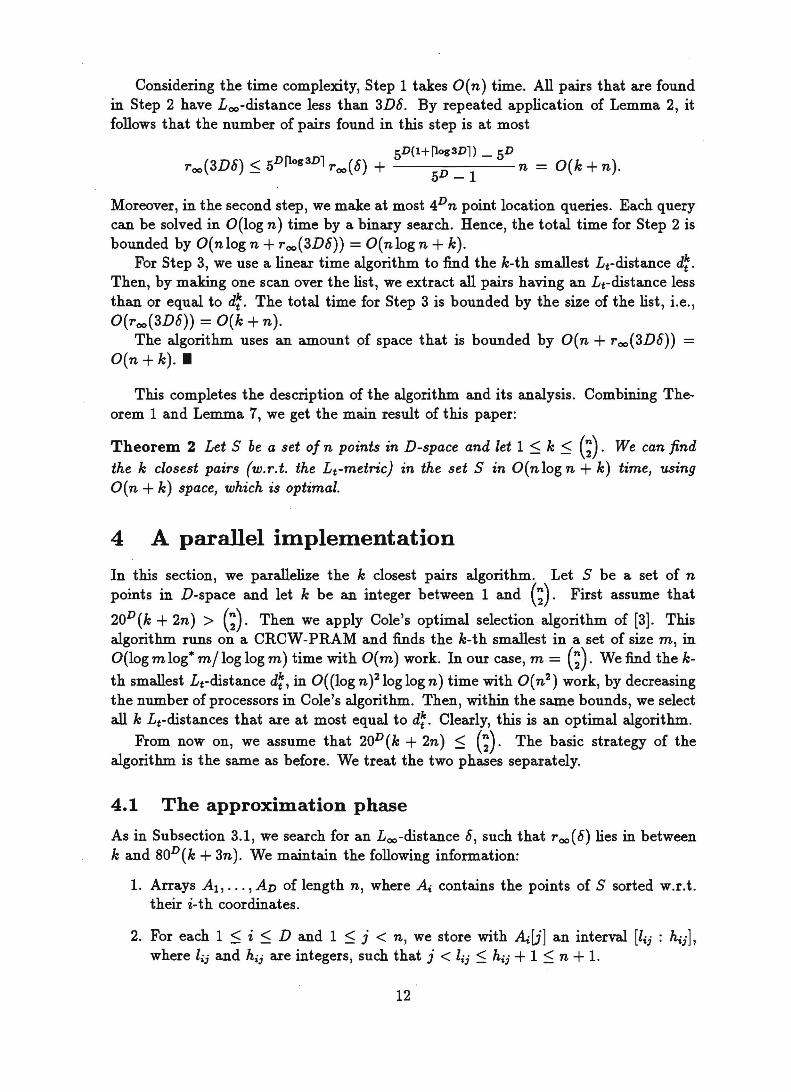
Considering the time complexity, Step 1 takes O( n) time. All pairs that are found . in Step 2 have Loo-distance less than 3Dh. By repeated application of Lemma 2, it follows that the number of pairs found in this step is at most

SD(l+rtog 3Dl) _ SD Too(3Dh) ~ sDrtog

3Dl Too(h) + ",n 1 n = O(k + n).

Moreover, in the second step, we make at most 4D n point location queries. Each query can be solved in O(log n) time by a binary search. Hence, the total time for Step 2 is bounded by O(nlog n + Too(3Dh)) = O(nlog n + k).

For Step 3, we use a linear time algorithm to find the k-th smallest Lt-distance d~. Then, by making one scan over the list, we extract all pairs having an Lt-distance less than or equal to d~. The total time for Step 3 is bounded by the size of the list, i.e., O(Too (3Dh)) = O(k + n).

The algorithm uses an amount of space that is bounded by O(n + Too (3Dh)) = O(n + k) .•

This completes the description of the algorithm and its analysis. Combining The­orem 1 and Lemma 7, we get the main result of this paper:

Theorem 2 Let S be a set 0/ n points in D-space and let 1 ~ k ~ (;). We ciln find the k closest pairs (w.r.t. the Lt-metric) in the set S in O(nlog n + k) time, using O(n + k) space, which is optimal.

4 A parallel implementation

In this section, we parallelize the k closest pairs algorithm. Let S be a set of n points in D-space and let k be an integer between 1 and (;). First assume that

20D (k + 2n) > (;). Then we apply Cole's optimal selection algorithm of [3]. This algorithm runs on a CRCW-PRAM and finds the k-th smallest in a set of size m, in O(log m log'" m/ log log m) time with O( m) work. In our case, m = (;). We find the k-th smallest Lt-distance d~ , in O( (log n )2 log log n) time with O( n 2) work, by decreasing the number of processors in Cole's algorithm. Then, within the same bounds, we select all k Lt-distances that are at most equal to d~. Clearly, this is an optimal algorithm.

From now on, we assume that 20D (k + 2n) ~ (;). The basic strategy of the algorithm is the same as before. We treat the two phases separately.

4.1 The approximation phase

As in Subsection 3.1, we search for an Loo-distance h, such that Too(h) lies in between k and 80D (k + 3n). We maintain the following information:

1. Arrays Al," ., AD of length n, where Ai contains the points of S sorted w.r.t. their i-th coordinates.

2. For each 1 ~ i ~ D and 1 ~ j < n, we store with ~[j] an interval [lij : h ij ],

where lij and h ij are integers, such that j < lij ~ h ij + 1 ~ n + 1.

12

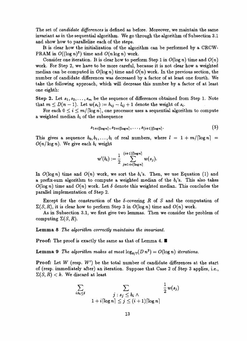
The set of candidate diJJerences is defined as before. Moreover, we maintain the same invariant as in the sequential algorithm. We go through the algorithm of Subsection 3.1 and show how to parallelize each of the steps.

It is dear how the initialization of the algorithm can be performed by a CRCW­PRAM in O((log n)2) time and O(nlog n) work.

Consider one iteration. It is dear how to perform Step 1 in O(1og n) time and O( n ) work. For Step 2, we have to be more careful, because it is not dear how a weighted median can be computed in O(1og n) time and O(n) work. In the previous section, the number of candidate differences was decreased by a factor of at least one fourth. We take the following approach, which will decrease this number by a factor of at least one eighth:

Step 2. Let SI, S2, .•• , Sm be the sequence of differences obtained from Step 1. Note that m ::; D(n - 1). Let W(Si) := hij -:-lij + 1 denote the weight of Si.

For each 0 ::; i ::; m/ flog n 1, one processor uses a sequential algorithm to compute a weighted median bi of the subsequence

sl+iflognl' S2+iflognl, .. . , S(i+1)flognl· (5)

This gives a sequence bo, bl , ... ,bz of real numbers, where 1 - 1 + m/ flog n 1 = O( n/ log n) . We give each bi weight

1 (i+l)flognl

w'(bi) := - L w(Sj). 2. ·fl 1 3=1+, ogn

In O(logn) time and O(n) work, we sort the b/s. Then, we use Equation (1) and a prefix-sum algorithm to compute a weighted median of the bi's. This also takes O(log n) time and O( n) work. Let ~ denote this weighted median. This condudes the parallel implementation of Step 2.

Except for the construction of the ~-covering R of S and the computation of ~(S, R), it is dear how to perform Step 3 in O(log n) time and O( n) work.

As in Subsection 3.1, we first give two lemmas. Then we consider the problem of computing ~(S, R).

Lemma 8 The algorithm correctly maintains the invariant.

Proof: The proof is exact1y the same as that of Lemma 4 .•

Lemma 9 The algorithm makes at most logs/T( D n2 ) = O(log n) iterations.

Proof: Let W (resp. W') be the total number of candidate differences at the start of (resp. immediately after) an iteration. Suppose that Case 2 of Step 3 applies, i.e., ~(S, R) < k. We discard at least

L i:b;$6

L j : Sj ::; bi 1\

1 2 w(Sj)

1 + i flog n 1 ::; j ::; (i + 1) flog n 1

13

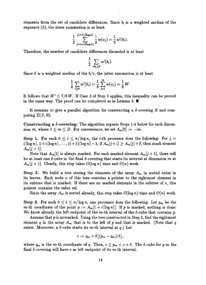
elements from the set of candidate differences. Since bi is a weighted median of the sequence (5), the inner summation is at least

1 (i+l)flognl 1 1 - I: -w(Sj)=-w'(bi ).

2 j=l+iflognl 2 2

Therefore, the number of candidate differences discarded is at least

1 2" . I: w'(bi ).

d.:56

Since 8 is a weighted median of the b/s, the latter summation is at least

11m. 1 - I:w'(bi ) = - I:w(Sj) = - w. 4 i>O 8 j=1 8

It follows that W' ~ 7/8 W. H Case 3 of Step 3 applies, this inequality can be proved in the same way. The proof can be completed as in Lemma 5 .•

It remains to give a parallel algorithm for constructing a 8-covering Rand com­puting :E(S, R).

Constructing a 8-covering: The algorithm repeats Steps 1-4 below for each dimen­sion m, where 1 ~ m ~ D. For convenience, we set Am.[O] := -00.

Step 1. For each 0 ~ i ~ n/ log n, the i-th processor does the following: For j = i [log n 1,1 +i[logn 1, ... , (i + 1) [log nl-1, if Am.[j + 1] ~ Am.[j] +8, then mark element Am.(j + 1].

Note that Am.[1] is always marked. For each marked element Am.[j + 1], there will be at least one 8-cube in the final 8-covering that starts its interval at dimension m at Am.(j + 1]. Clearly, this step takes O(log n) time and O(n) work.

Step 2. We build a tree storing the elements of the array Am. in sorted order in its leaves. Each node v of this tree contains apointer to the rightmost element in its subtree that is marked. If there are no marked elements in the subtree of v, this pointer contains the value nil.

Since the array Am is sorted already, this step takes O(1og n) time and O( n) work.

Step ~. For each 0 ~ i ~ n/ log n, one processor does the following: Let Pm be the m-th coordinate of the point P := Am.[1 + i [log nl]· If pis marked, not hing is done: We know already the left endpoint of the m-th interval of the 8-cube that contains p.

Assume that pis unmarked. U sing the tree constructed in Step 2, find the rightmost element q in the array Am. that is to the left of p and that is marked. (N ote that q

exists. Moreover, a 8-cube starts its m-th interval at q.) Let

c:= qm + 8L(Pm - qm)/8J,

where qm is the m-th coordinate of q. Then, c ~ pm < C + 8. The 8-cube for p in the final 8-covering will have c as left endpoint of its m-th interval.

14

How do we compute L(Pm - qm)j8J? We know that all elements in Am that are between q and P are unmarked. That is, the difference of the m-th coordinates of two consecutive elements between q and P is less than 8. Therefore, 0 < pm - qm < n8, which implies that 0 :'S L(Pm - qm)j8J < n. We compute this integer in O(log n) time by binary search. In this way, we only use algebraic functions.

At this moment, the i-th processor knows the left endpoint of the m-th interval of the 8-cube to which P = Am [1 + i flog n II belongs. This processor uses Step 1 of the sequential algorithm of Subsection 3.1-for dimension m-to find 8-intervals for the points Am[l + i flog n ll, Am [2 + i flog n ll,· .. , Am [(i + 1) flog n 1].

Step 3 takes O(logn) time and O(n) work. At the end of this step, we know for each point the left boundary of the m-th interval of its 8-cube. Moreover, since Am is sorted, we have these left boundaries in sorted order.

Step 4. We rank the n left boundaries obtained from the previous step. (Equal boundaries get the same rank.) This takes O(log n) time and O( n) work.

At the end of this step, we have for each point the number of its 8-slab for the m-th dimension. (These slabs are numbered starting at one.)

Step 5. Note that we have carried out the first four steps for each dimension. There­fore, at this moment, each point has stored with it two vectors oflength D. If point P has vectors (Cl, C2, ••• , CD) and (kI, k2 , ••• , kD ), then P is contained in the 8-cube with lower-Ieft corner (Cl, C2, ••• ,CD). This 8-cube is part of the km-th 8-slab along the m-th a.x:J.S.

These vectors implicitly define the 8-covering R. So, it remains to compute E( S, R). Note that each km is an integer in the range from 1 to n. We consider each vector (kl , k2 , ••• , kD) as an integer between 1 and nD+1. Then, using the randomized algo­rithm of Matias and Vishkin [9, Theorem 3], we sort these integers. On a CRCW­PRAM, this takes O(log n log log n) expected time and O( n log log n) work.

Given this sorted sequence, we compute how often each value occurs. Then, we can compute E( S, R). This takes O(1og n) time and O( n) work.

Lemma 10 Let R be the set 01 hypercubes that are computed by the above algorithm. Then, R is a 8-covering 01 S. Moreover, the algorithm computes Rand E( S, R) in O(log n log log n) expected time and O( n log log n) work.

Proof: The proof follows from the above discussion .•

Theorem 3 There exists a CRCW-PRAM algorithm that computes areal number 6 such that k :'S r oo( 8) :'S 80D (k + 3n). The algorithm takes O( (log n )2 log log n) expected time and O( n log n log log n) work.

Proof: The correctness of the algorithm follows in the same way as in Theorem 1. The initialization of the algorithm takes O((log n)2) time and O(nlog n) work. Combining this with Lemmas 9 and 10, the complexity bounds follow .•

15

4.2 The enumeration phase

The parallelization of the enumeration phase follows easily form the sequential algo­rithm of Subsection 3.2. In Step 1-construction of the Dc5-covering R of S-we use Steps 1-3 of the procedure in the. previous subsection. This gives for each point p a vector of length D indicating the lower-Ieft corner of the c5-cube of R that contains p. Then, we use any optimal sorting algorithm to sort these cubes, more precisely, the lower-Ieft corners of these cubes. Hence, Step 1 of the enumeration phase takes O«log n )2) time and O( n log n) work.

The sorted sequence of c5-cubes allows us to do point location in logarithmic time. (Note that we basically apply the slab method for point location.) In Step 2, .we find the same O( k + n) pairs as in Step 2 of Subsection 3.2. This takes O( (log n )2 log log n) time and O( n log n + k) work.

For Step 3, we use Cole's optimal algorithm of [3] that finds the k-th smallest element in the list of O( k + n) Lt-distances. This algorithm takes O( (log n )2 log log n) time and O( n + k) work. Given this k-th smallest distance d~, we select all k Lt -

distances that are at most equal to d~. This also takes O( (log n )2 log log n) time and O(n + k) work.

Lemma 11 Given the real number c5 0/ Theorem 9, we can find the k closest pairs in the set S in O( (log n )2 log log n) time and O( n log n + k) work.

Proof: The correctness proof is the same as in Lemma 7. The complexity bounds follow from the description just given .•

This condudes the description of our parallel k dosest pairs algorithm. We combine Theorem 3 and Lemma 11 to obtain the following result.

Theorem 4 Let S be a set 0/ n points in D-space and let 1 :s; k :s; (;). There exists a CRCW-PRAM algorithm that finds the k closest pairs (w.r.t. the Lt-metric) in the set S in O( (log n? log log n) expected time and O( n log n log log n + k) work.

Of course, we can use the algorithm with k = 1 to find the dosest pair in the set S. For dimensions that are greater than two, this gives the currently best result:

Corollary 3 Let S be a set 0/ n points in D-space. There exists a CRCW-PRAM algorithm thatfinds the closest pair (w.r.t. the Lt-metric) in S in O((logn?loglogn) expected time and O( n log n log log n) work.

5 Concluding remarks

We have given an optimal sequential algorithm for the k dosest pairs problem. As mentioned already, the constants that appear are rather high. They are valid, however, for any Lt-metric, 1 :s; t :s; 00. By a more careful analysis, the constants can be improved. In particular, by taking a specific t, e.g. t - 2, in which case we consider the Euclidean metric, it is easy to improve them. They remain, however, of the form ~logD.

16

There remain some interesting problems that need more attention. Dur algorithm approximates the Loo-distance with a certain rank r. Can it be modified to find the exact Loo-distance with rank r? Note that Salowe [10] solves this problem in O( n(log n )D) time. Another problem is to find the Lt-distance with rank r for other values of t.

The algorithm presented here finds the k smallest distances, but it does not output this sequence in sorted order. Of course, we can solve the "sorted k closest pairs problem" in 0(( n + k) log n) time. It is an open problem if the time complexity can be

improved to O(nlog n + k). In particular, it is an open problem if we can sort all (;)

distances in O(n2 ) time. Finally, can we use the techniques of this paper to improve the time bounds in [7] for

the k furthest pairs problem, or for the k closestjfurthest bichromatic pairs problem? (N ote that the results in [7] only hold for the plan ar case.)

For the parallel version of the algorithm, the product of the time complexity and the number of processors is O( n log n log log n + k). It would be interesting to re­move the log log n-factor from this product. Note that this factor comes from integer sorting. Hence, any improvement for this problem leads to an improvement of our algorithm. Moreover, it would be interesting to remove randomization from this algo­rithm. Finally, it is an open problem to devise an optimal parallel algorithm for the higher-dimensional closest pair problem, i.e., for the case k = 1.

Acknowledgement

The authors thank Torben Hagerup and Christine Rüb for their help with the parallel version of the algorithm.

References

[1] P.K. Agarwal, B. Aronov, M. Sharir and S. Suri. Selecting distances in the plane. Proc. 6-th ACM Symp. on Comp. Geom., 1990, pp. 321-331.

[2] J.L. Bentley and M.I. Shamos. Divide-and-conquer in multidimensional space. Proc. 8-th Annual ACM Symp. on Theory of Computing, 1976, pp. 220-230.

[3] R. Cole. An optimally efficient selection algorithm. Information Processing Letters 26 (1988), pp. 295-299.

[4] R. Cole and M.T. Goodrich. Optimal parallel algorithms for point-set and polygon problems. Algorithmica 7 (1992), pp. 3-23.

[5] M.T. Dickerson and R.S. Drysdale. Enumerating k distances for n points in the plane. Proc. 7-th ACM Symp. on Comp. Geom., 1991, pp. 234-238.

[6] D.B. Johnson and T. Mizoguchi. Selecting the Kth element in X + Y and Xl + X 2 + ... + X m • SIAM J. Comput. 7 (1978), pp. 147-153.

17

[7] N. Katoh and K. Iwano. Finding k farthest pairs and k closest/farthest bichro­matic pairs for points in the plane. Proc. 8-th ACM Symp. on Comp. Geom., 1992, pp. 320-329.

[8] H.P. Lenhof and M. Smid. The k closest pairs problem. Unpublished manuscript, 1992.

[9] Y. Matias and U. Vishkin. On parallel hashing and integer sorting. J. of Algo­rithms 12 (1991), pp. 573-606.

[10] J.S. Salowe. L-infinity interdistance selection by parametrie search. Inform. Proc. Lett. 30 (1989), pp. 9-14.

[11] J.S. Salowe. Enumerating interdistances in space. Internat. J. Comput. Geom. Appl. 2 (1992), pp. 49-59.

[12] C. Schwarz, M. Smid and J. Snoeyink. An optimal algorithmfor the on-line closest pair problem. Proc. 8-th ACM Symp. on Comp. Geom., 1992, pp. 330-336.

[13] MJ. Shamos and D. Hoey. Closest-points problems. Proc. 16-th Annual IEEE . Symp. on Foundations of Computer Science, 1975, pp. 151-162.

[14] M. Smid. Maintaining the minimal distance of a point set in less than linear time. Algorithms Review 2 (1991), pp. 33-44.

[15] P.M. Vaidya. An O(nlog n) algorithm for the all-nearest-neighbors problem. Dis­crete Comput. Geom. 4 (1989), pp. 101-115.

18