Maximo Camacho and Gabriel Perez-Quiros fileÑ-STING: ESPAÑA SHORT TERM INDICATOR OF GROWTH (*) Maximo Camacho UNIVERSIDAD DE MURCIA Gabriel Perez-Quiros BANCO DE ESPAÑA AND CEPR

Ñ-STING: ESPAÑA SHORT TERM INDICATOR OF GROWTH

Maximo Camacho and Gabriel Perez-Quiros

Documentos de Trabajo N.º 0912

2009

Ñ-STING: ESPAÑA SHORT TERM INDICATOR OF GROWTH

Ñ-STING: ESPAÑA SHORT TERM INDICATOR OF GROWTH (*)

Maximo Camacho

UNIVERSIDAD DE MURCIA

Gabriel Perez-Quiros

BANCO DE ESPAÑA AND CEPR

(*) We thank the members of the Department of Coyuntura y Previsión for their suggestions and comments. The conversations with them have been extremely helpful to identify the relevant issues concerning forecasting growth in the Spanish economy. We also thank Juan Peñalosa for his detail comments on the first version of the paper. Maximo Camacho thanks the Fundación Ramón Areces for its financial support. The views expressed here are those of the authors and do not represent the views of the Bank of Spain or the Eurosystem

Documentos de Trabajo. N.º 0912

2009

The Working Paper Series seeks to disseminate original research in economics and finance. All papers have been anonymously refereed. By publishing these papers, the Banco de España aims to contribute to economic analysis and, in particular, to knowledge of the Spanish economy and its international environment. The opinions and analyses in the Working Paper Series are the responsibility of the authors and, therefore, do not necessarily coincide with those of the Banco de España or the Eurosystem. The Banco de España disseminates its main reports and most of its publications via the INTERNET at the following website: http://www.bde.es. Reproduction for educational and non-commercial purposes is permitted provided that the source is acknowledged. © BANCO DE ESPAÑA, Madrid, 2009 ISSN: 0213-2710 (print) ISSN: 1579-8666 (on line) Depósito legal: Unidad de Publicaciones, Banco de España

Abstract

We develop a dynamic factor model to compute short term forecasts of the Spanish GDP

growth in real time. With this model, we compute a business cycle index which works well as

an indicator of the business cycle conditions in Spain. To examine its real time forecasting

accuracy, we use real-time data vintages from 2008.02 through 2009.01. We conclude that

the model exhibits good forecasting performance in anticipating the recent and sudden

downturn.

JEL Classification: E32, C22, E27.

Keywords: Business Cycles, Output Growth, Time Series.

BANCO DE ESPAÑA 9 DOCUMENTO DE TRABAJO N.º 0912

1 Introduction

Due to the recent economic disturbances affecting the world economy, there has been an

explosive interest in the early assessment of the short term evolution of economic activity.

The academic literature and the press are full of references to short term GDP growth rate

forecasts and its successive revisions which are currently deteriorating with the ongoing

economic developments. However, the vast majority of the forecasts released by relevant

institutions do not always make explicit the methodology followed to compute their forecasts.

Therefore, it is difficult to replicate and intuitively understand the forecasts. In fact, the

forecasts of many of these institutions explicitly or implicitly rely on the judgment of experts,

which might be helpful in terms of increase the precise of their forecast, but implies two

serious drawbacks. The first drawback is that judgments make the forecasting process a

black box which becomes only clear to the mind of the forecaster. The second drawback is

that forecasts that rely on judgments make the forecasting process a subjective exercise

instead of an objective quantitative and measurable analysis. In that sense, forecasters may

read the news, and be affected by a general climate that may or may not be accurate to

describe the current economic situation. But at the same time, forecasters may even affect

the news and therefore, may contribute to create expectations which, if they are not

objectively quantifiable, may be only a partial description of the economic situation. In order

to avoid these problems, we propose in this paper a judgment-free algorithm which

automatically computes the forecasts when new information becomes available. In that

sense, our algorithm has the same advantages than the judgmental forecast in terms of the

ability to adapt to new information, but it avoids the serious inconveniences mentioned

before. The forecasting method is easy to interpret, easy to replicate, and easy to update.

Regarding the automatic forecasting methods, the most familiar are the standard

time series processes popularized by Box and Jenkins and their posterior refinements,

including multivariate time series process and error correction models. To predict GDP, these

models usually rely on quarterly series which are usually published with a delay which ranges

from about 45 to 60 days. Therefore, as of today, January 25th 2009, when forecasting next

quarter of GDP growth (second quarter of 2009) the standard time series models would use

data corresponding to the third quarter of 2008. These forecasts, apart from not capturing

the abrupt economic changes occurred in the fourth quarter of 2008 and the first month of

2009, will be subject to strong revisions in the reference series. With this outdated information

the standard autoregressive models usually exhibit strong mean reverting and their forecasts

are therefore seriously biased towards the mean which may lead to misleading forecasts in an

environment of economic turbulences.

To diminish this problem, we use a dynamic factor model which uses economic

indicators that are related to GDP growth but are much promptly published. One potential

alternative specification could be based on transfer functions which include the set of

indicators as explanatory variables. However, estimating these models is problematic when

the number of indicators increases. For these reasons, dynamic factor models become the

most appropriate framework to compute the forecasts. These specifications are based

on the assumption that the joint dynamics of GDP growth and the indicators can be

decomposed in two components. For each of these series, the first component refers

to the common dynamics whereas the second component refers to its idiosyncratic

dynamics.


In the recent empirical literature, two alternative dynamic factor models are used.

One is the factor models that are based on large sets of economic indicators which are

estimated by using approximate factor models as in Angelini et al. (2008) for Euro-area data

and by Camacho and Sancho (2003) for Spanish data. The other alternative relies on previous

reasonable pre-screenings of the series which are estimated by using strict factor models and

has recently been applied by Camacho and Perez-Quiros (2008) and by Frale, Marcellino,

óMazzi and Proietti (2008) to Euro-area data. Regarding the controversy between using

large versus small scale factor models, it has been pointed out by Boivin and Ng (2006) that

the asymptotic advantages of large-scale factor models are frequently far from being held

in empirical applications. In addition, Alvarez-Aranda, Camacho and Perez-Quiros (2009)

examine the empirical pros and cons of forecasting with large versus small factor models. The

main result of this line of research is that, in empirical applications, the larger is the number of

time series, the higher is the correlation of the idiosyncratic part, and this correlation might

bias the results of the estimated common factor. Therefore, according to these authors,

more is not always better from a forecasting point of view. In addition, Bai and Ng (2008) have

shown the importance of having parsimonious specifications in order to improve the

forecasting ability of factor models, even when zero cross-correlation among the idiosyncratic

part holds.

In line with the previous discussion, we propose a small scale factor model to

compute short term forecasts of the Spanish GDP growth rate in real time. The model

is constructed to deal with the typical problems affecting real-time economic releases. First,

the model deals with ragged edges in order to take into account all the available information

which is released in a non-synchronous way. Second, the model accounts for data with

mixed frequencies, in order to bridge monthly indicators with quarterly GDP. Third, the model

is a simple algorithm that can be automatically updated, so the model handles with

potential economic instabilities, because, if the predictive power of any variable diminishes

during the course of some periods, the variable will reduce its weight and its loading factor.

Finally, the model is dynamically complete in the sense that accounts for the dynamics of all

the indicators used in the analysis. This leads the model to be a metric to measure the news

associated with each realization of the indicators used in the analysis, based on the effect that

each realization has on the expected economic growth.

The empirical reliability of the model is evaluated by using both in-sample data

from 1990.01 to today and real-time data from February 2008 to today. This exercise

describes the main outputs that are obtained by the model in each of the automatized

forecasts. The outputs show that the factor works reasonably well as an indicator of the

recent economic evolution in Spain. As expected, the loading factors are positive and

statistically significant which reinforces the standard view that the indicators are procyclical.

In addition, as in Banbura and Runstler (2007) or Camacho and Perez-Quiros (2008), the

empirical results show that a suitable treatment of publication lags may lead some indicators

to provide important sources of information in predicting GDP beyond the information

provided in the in-sample estimates of the loading factors.

The paper is organized as follows. Section 2 outlines the proposed methodology.

Section 3 evaluates the empirical reliability of the model. Section 4 concludes.


2 Description of the model

In this section we develop the model to compute short term forecasts of the Spanish GDP

growth in real time from a set of indicators that may include mixing frequencies and missing

data.

2.1 Selection of indicators

The series used in the estimation of the model are listed in Table 1. The selection of these

variables is based on the model suggested by Stock and Watson (1991). Their idea

follows the logic of national accounting by computing GDP from the income side, the

supply side and the demand side. Therefore, to obtain robust estimates of activity with

a monthly frequency they choose industrial production index (supply side), total sales

(demand side), real personal income (income side) and they add an employment variable

to capture the idea that productivity do not change dramatically from one period to the other.

Since we do not have for the Spanish economy a reliable income variable, we start

the selection of indicators with Industrial Production (excluding construction), total sales of

large firms of Agencia Tributaria (Spanish Internal Revenue Service) and social security

contributors.

However, as pointed out in Camacho and Perez-Quiros (2008) the delay in the

publication of some of these series (see Table 1), and the serious revisions that some of them

are subject to, makes it difficult to follow the real time economic evolution with only these

three indicators. Following their paper, we extend Stock-Watson initial set of indicators set

in two dimensions. On the one hand we include soft indicators series that have the property

of being early indicators of activity available with almost no publication delays. From the

supply side, we choose the Industrial Confidence Indicator as an Index of the production

sector, and the PMI services for the production of the services sector. From the demand side,

we choose the Retail sales Confidence Index. We estimate this model, and the model fit the

GDP data very precisely. In particular, in line with these authors we evaluate the fit of

the model by computing the proportion of variance of GDP explained by the common factor.

In this model, this proportion reaches 79%.

According to Camacho and Perez-Quiros (2008) we decide to include more

variables into the model if the variance of GDP explained by the factor increases with the

inclusion of additional variables. Contrary to standard lineal techniques when more variables

always increase the variance explained by the model, this is not always true in this type of

models. In particular, when the additional variables are correlated with the idiosyncratic part

of some of the variables, the estimation of the factor is biased toward this subgroup, making

the variance of GDP explained by the factor to decrease.

With this criterion in mind, we use the knowledge about the Spanish economy which

is accumulated in the Bank of Spain and enlarge the set of indicators with some key

economic variables of the Spanish economy. The idea is to include, on the supply side, not

only and indicator of the manufacturing sector, (industrial production) but also an indicator of

the services sector (overnight stays) and construction sector (consumption of cement). On the

demand side, we include not only internal demand (total sales) but also external demand

(import and export). The enlarged model has a variance of GDP explained by the factor

increases to 80%.


It is worth noting that we tried to enlarge the set of indicators with other economic

variables but we always obtained reductions in the percentage of the variance GDP that was

explained by the factor. This was the case when we added more series of the Agencia

Tributaria such as wages paid by large firms, exports of large firms and imports of large firms.

In addition, we failed to improve the variance of GDP explained by the factor when we added

disaggregated versions of the variables already included in the model as was the case of

some components of industrial production. We also finally added series such a stock market

returns or interest rates which were too noisy to improve the accuracy in the estimation of

GDP obtained by the common factor.

One final remark regarding the indicators is that most of the hard indicators are

extremely noisy taken in monthly growth rates. In order to smooth that noise without filtering

out the data with HP or band pass filters, we include these series in the model in annual

growth rates.1 Additionally, soft indicators are usually considered in levels, because according

to the European Comission, these indicators are designed to capture annual growth rates of

the series of interest. The unit root problems associated with the annual growth rates and the

levels of the soft indicators are solved by specifying the model with a monthly factor,

but taking into account that the indicators are function of current and up to eleven lags of

this factor.2

The following two subsections are the description of the econometric methodology

which is similar to that used in the Euro-Sting model of Camacho and Perez-Quiros (2008).

Readers which are familiar to that model can skip these sections.

2.2 Mixing quarterly and monthly observations

The model is based on the idea of obtaining early estimates of quarterly GDP growth by

exploiting the information in monthly indicators which are promptly available. Linking monthly

data with quarterly observations needs to express quarterly growth rates observations as the

evolution of monthly figures.

For this purpose, let us assume that the levels of the quarterly GDP can be

decomposed as the sum of three unobservable monthly values of GDP. Mariano and

Murasawa (2003) show that if the sample mean of these three data can be well approximated

by the geometric mean, the quarterly growth rate of GDP can be expressed as the average of

monthly growth rates of latent observations:

4321 32

31

31

32

−−−− ++++= tttttt xxxxxy

It is worth saying that approximating sample means with geometric means is

appropriate since the evolution of macroeconomic series is smooth enough to allow for

this approximation. In related literature, Proietti and Moauro (2006) avoid this approximation

at the cost of moving to a complicated non-linear model. Aruoba, Diebold and Scotti (2009)

1. Just because it is a common practice, we use seasonally and calendar adjusted data. The model is robust to

estimation with raw data.

2. See Camacho and Perez-Quiros (2008) for further details in data transformation.


also avoid the approximation but assuming that the series evolve as deterministic trends

without unit roots.3

2.3 Bridging with factors

The practical application of the procedure described in the previous section exhibits

two econometric problems. The first problem is that the procedure is specified in

monthly frequencies. This implies the need to estimate unobserved components such

as monthly growth rates and quarterly growth rates for the first two months of each quarter.

The second problem is that the model has to handle with many missing observations

since some series start too late, and some series (those with longer publication delays)

end too soon.

Dynamic factor models are the appropriate framework to deal with these drawbacks.

These are also good models to characterize comovements in macroeconomic variables

that admit factor decompositions. The single-index dynamic factor model is based on the

premise that the dynamic of each series can be decomposed into two orthogonal

components. The first component, called common component and denoted by ft,

captures the collinear dynamics affecting all the variables and can be interpreted as

a coincident indicator of the GDP growth rate. The second component, called idiosyncratic

component and denoted for each indicator j by ujt, captures the effect of those dynamics

which only affect that particular variable.

Let xt be the monthly GDP growth rate and let zt be the k-dimensional vector of

economic indicators in monthly growth rates (hard indicators) or levels (for soft indicators).4

The model can then be stated as

⎟⎟⎠

⎞⎜⎜⎝

⎛+=⎟⎟

⎠

⎞⎜⎜⎝

⎛

zt

ytt

t

t

uu

fzx

β (1)

where ( )ktttzt uuuu ,...,, 21= . The (k+1) parameters in β are known as the factor loadings

and capture the correlation between the unobserved common factor and the variables.

To complete the statistical representation of the model, we assume the following dynamic

specification for the variables.

( ) ytyty uL εφ = , (2)

( ) ftftf uL εφ = , (3)

( ) k,...,i ,uL ititi 1== εφ , (4)

3. In the most recent extension of their model, Arouba and Diebold (2009) abandon their exact filter and use the

approximate filter by taking growth rates of the time series.

4. Indicators in levels create the problem of mixing integrated and stationary variables in the same specification.

We solve the problem by considering, as pointed out in the works of the European Commission, that soft indicators

are related with annual growth rates of the variable of interest, therefore, the level of the soft indicators depend on

a 12 month moving average of the common factor, and this is the source of its unit root.


where ( )Lyφ , ( )Lfφ , and ( )Liφ are lag polynomials of order p, q and r, respectively.

In addition, we consider that all the errors in these equations are independent and

identically normal distributed with zero mean and diagonal covariance matrix.

Dealing with balanced panels, i.e, when all the variables are observed in each period,

the model can be easily stated in state space representation which can be estimated by

maximum likelihood procedures [see Hamilton (1999) and references therein]. In addition,

the Kalman filter is the natural statistical method to deal with missing observations. Following

Mariano and Murasawa (2003), we substitute the missing observations with random draws

(means, medians or zeroes are also valid alternatives). The substitutions allow the matrices in

the state-space representation to be conformable but they have no impact on the model

estimation since the missing observations add just a constant in the likelihood function

to be estimated by the process.

The model can be written in state space form. Let us collect the quarterly growth

rates of GDP and the annual growth rates of the ten indicators in the vector ( )''ttt z,yY = , and

their idiosyncratic components in the vector ( )''ztytt u,uu = . The observation equation is

ttt wHsY += , (5)

where ( )RiNwt ,0~ . The transition equation is

ttt vFss += −1 , (6)

where ( )QiNvt ,0~ .

The details about the specific form of the matrix H when dealing with quarterly

growth rates and annual growth rates of monthly indicators and indicators in levels are

described in the appendix.

One interesting result from dynamic factor models are the weights or cumulative

impact of each indicator to the forecast GDP growth and can be obtained from the

Kalman filter. Skipping details, the state vector st can be expressed as the weighted sum

of available observations in the past.5 Assuming a large enough t such that the Kalman

filter has approached its steady state it holds that h-period ahead forecasts of GDP growth

are approximately

∑=∞

=−+

0jjt

'jht YWy

In this expression, Wj is the vector of weights and leads the forecaster to compute

the cumulative weight of series i in forecasting GDP growth as ( )∑∞

=0jj iW , where Wj(i) is the i-th

element of Wj.

5. See Stock and Watson (1991) for further details.


3 Empirical analysis

In this section, the model is used to compute in-sample maximum likelihood estimates which

are intuitively interpreted. In addition, the model is applied to the real-time vintages of data

sets from 2008.02 through 2009.01 to examine its accuracy in accounting for the recent and

sudden downturn.

3.1 In-sample results

The in-sample dataset which is available on January 25, 2009 includes data from 1990.01 to

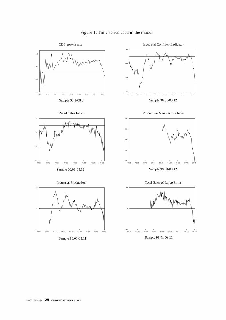
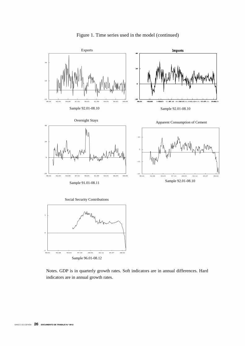
2008.12, and it is depicted in Figure 1.6 The key series to be forecasted is quarterly growth

rate which starts in 1992.1 and ends in 2008.3 and is plotted in the first graph. Some of the

ten indicators used in the model are shorter time series since they started to be published

in the mid nineties. The three soft indicators, which are based on survey data, are plotted in

levels in graphs 2 to 4. The last seven graphs show the evolution of hard indicators which are

plotted in annual growth rates. Despite the particularities exhibited in their evolution, all of

them seem to share a common pattern with two significant slowdowns at the beginning and

at the end of the sample.

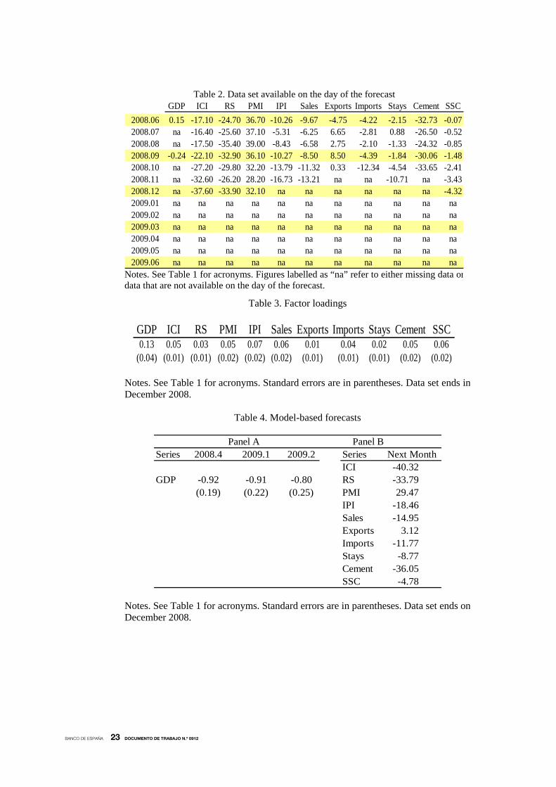
The particular publication pattern of these series can be examined in Table 2 which

shows the last figures of the time series. Since GDP is published quarterly, the two first

months of each quarter are treated as missing data. Typically, surveys have very short

publishing lags since they are frequently published within the current month while hard data

are released with a relatively longer delay of about two months. We put nine months of

missing data after the last GDP growth observation because this is the horizon of our

predictions In January 2009, the last available release of GDP was in September 2008 and

from this date until June 2009 the Kalman filter employed in the model will fill in these missing

observations by computing dynamic forecasts for the last quarter of 2008 and the first two

quarters of 2009. Accordingly, the nine-month forecasting horizon will be moved forward

when GDP for the last quarter will be actually published.

The model adopted in this paper is based on the notion that comovements among

the macroeconomic variables have a common element, the common factor, which moves

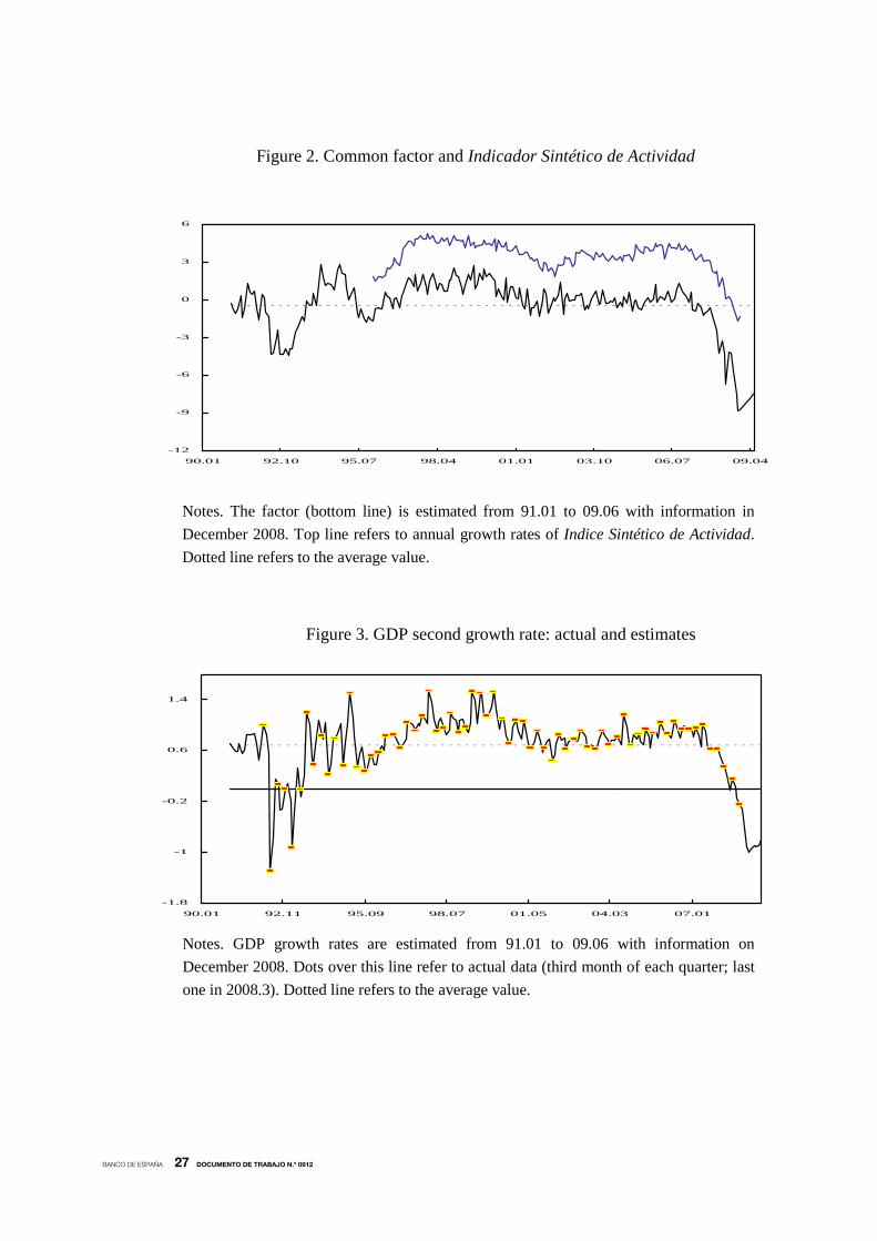
according to the Spanish business cycle dynamics. In this context, Figure 2 shows the

estimated factor (bottom line) and the annual growth rates of the Synthetic Index of Economic

Activity (Indicador Sintético de Actividad Económica, top line) which is elaborated by the

Spanish Ministry of Economy since 1995 to account for the recent economic evolution

in Spain. It is clear that the business cycle fluctuations of these two time series are in close

agreement which validates the view that our factor agrees with the dynamics of the Spanish

economic activity.

Skipping details, the indicator starts the nineties on its average value (dotted line) and

suffers from the first temporary drop in 1992 and 1993. After the summer 1993, the indicator

increased substantially and reached above-average values until mid nineties, when a milder

drop characterized the winter 1995/96. Apart from a mild slowdown in 2001, during the next

decade and until 2008 the indicator is uninterruptedly either on or above the average and

its flatted trend marks the period of high growth which characterizes the Spanish economy in

6. To understand notation, for example 2008.1 or 08.1 refer to first quarter of year 2008 while 2008.01 or 08.01 refer to

first month of year 2008.


those years. At the beginning of 2008, there is marked breakpoint in the evolution of the

factor. The figures of the indicator turned to negative and the pattern followed by the indicator

became clearly negative trended. It is worth noting that, in terms of abruptness and

deepness, the trend observed in all the economic indicators but exports are in line with the

trend marked by the factor. Using the information up to January 2009, signals of recoveries

are not expected by the model predictions at least until the end of 2009.

To examine the correlation of the indicators and the factor, Table 3 shows the

maximum likelihood estimates of the factor loadings (standard errors within parentheses).

Apart from GDP, the economic indicators with larger loading factors are those corresponding

to Industrial Production Index, Total Sales of Large Firms, Social Security Contributors, and

Production Manufacture Index. The indicator with lower correlation with the latent common

factor is exports (and to less extent, Overnight Stays) which it is only marginally significant.7

However, the estimates are always positive and statistically significant, indicating that these

series are procyclical, i.e., positively correlated with the common factor. One final remark

is the positive correlation between imports and the factor. Contrary to the standard view in

national accounting, imports are interpreted within the model as an indicator of final demand,

and therefore have a procyclical behavior.

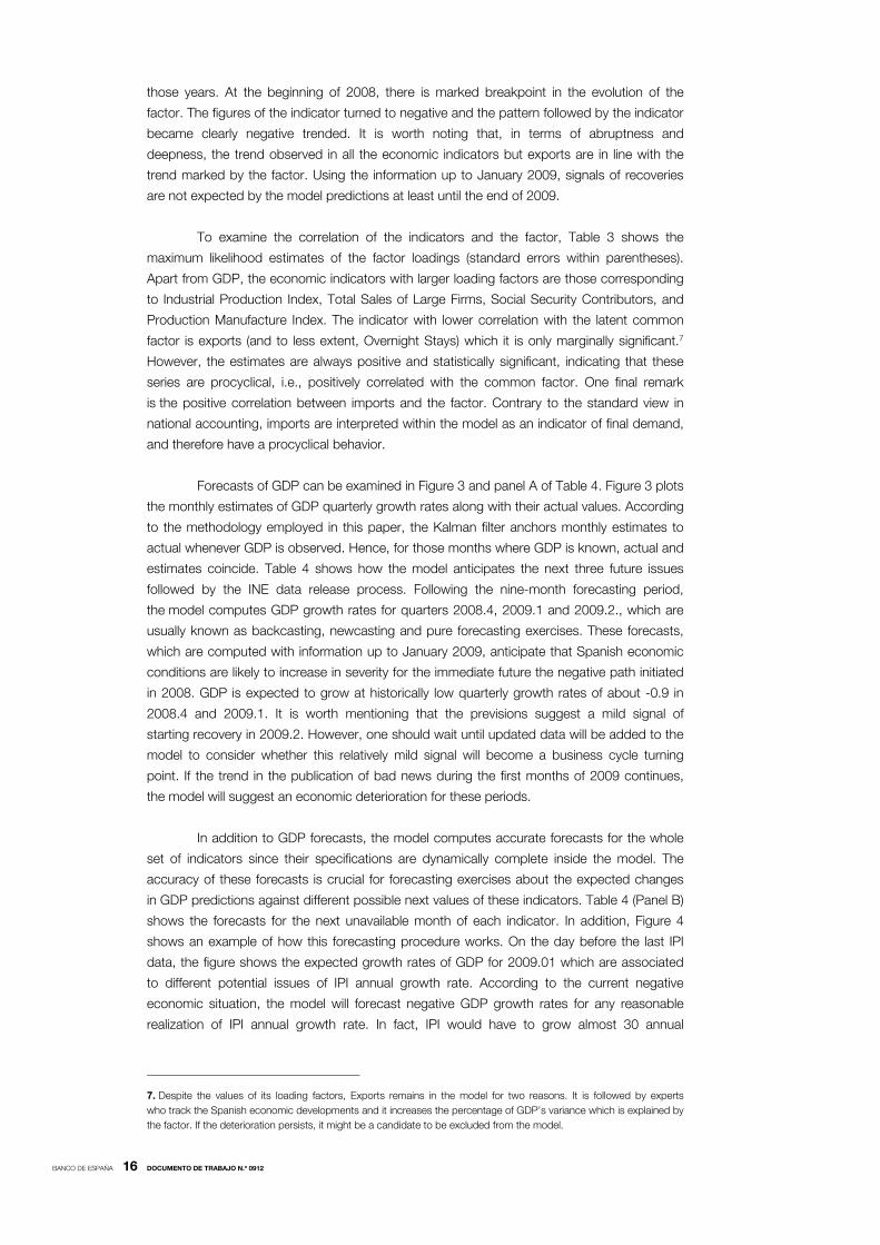
Forecasts of GDP can be examined in Figure 3 and panel A of Table 4. Figure 3 plots

the monthly estimates of GDP quarterly growth rates along with their actual values. According

to the methodology employed in this paper, the Kalman filter anchors monthly estimates to

actual whenever GDP is observed. Hence, for those months where GDP is known, actual and

estimates coincide. Table 4 shows how the model anticipates the next three future issues

followed by the INE data release process. Following the nine-month forecasting period,

the model computes GDP growth rates for quarters 2008.4, 2009.1 and 2009.2., which are

usually known as backcasting, newcasting and pure forecasting exercises. These forecasts,

which are computed with information up to January 2009, anticipate that Spanish economic

conditions are likely to increase in severity for the immediate future the negative path initiated

in 2008. GDP is expected to grow at historically low quarterly growth rates of about -0.9 in

2008.4 and 2009.1. It is worth mentioning that the previsions suggest a mild signal of

starting recovery in 2009.2. However, one should wait until updated data will be added to the

model to consider whether this relatively mild signal will become a business cycle turning

point. If the trend in the publication of bad news during the first months of 2009 continues,

the model will suggest an economic deterioration for these periods.

In addition to GDP forecasts, the model computes accurate forecasts for the whole

set of indicators since their specifications are dynamically complete inside the model. The

accuracy of these forecasts is crucial for forecasting exercises about the expected changes

in GDP predictions against different possible next values of these indicators. Table 4 (Panel B)

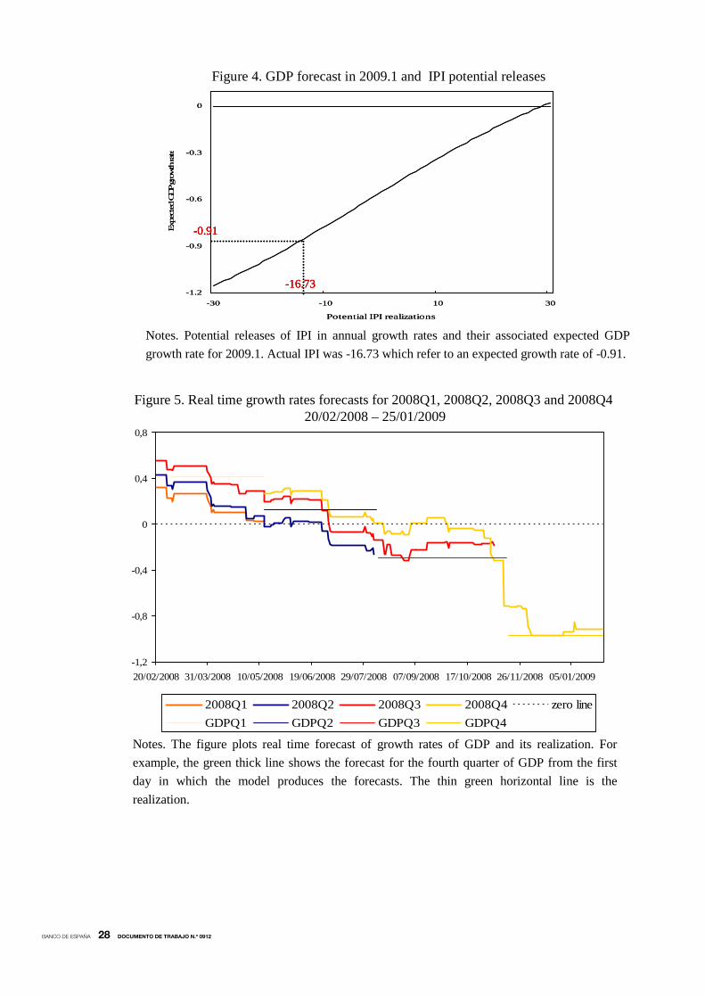
shows the forecasts for the next unavailable month of each indicator. In addition, Figure 4

shows an example of how this forecasting procedure works. On the day before the last IPI

data, the figure shows the expected growth rates of GDP for 2009.01 which are associated

to different potential issues of IPI annual growth rate. According to the current negative

economic situation, the model will forecast negative GDP growth rates for any reasonable

realization of IPI annual growth rate. In fact, IPI would have to grow almost 30 annual

7. Despite the values of its loading factors, Exports remains in the model for two reasons. It is followed by experts

who track the Spanish economic developments and it increases the percentage of GDP’s variance which is explained by

the factor. If the deterioration persists, it might be a candidate to be excluded from the model.


percentage points to convert the IPI signal into positive forecasts of GDP growth rate.

The actual IPI figure was -16.73 and this value implied a forecast of GDP growth of -0.91.

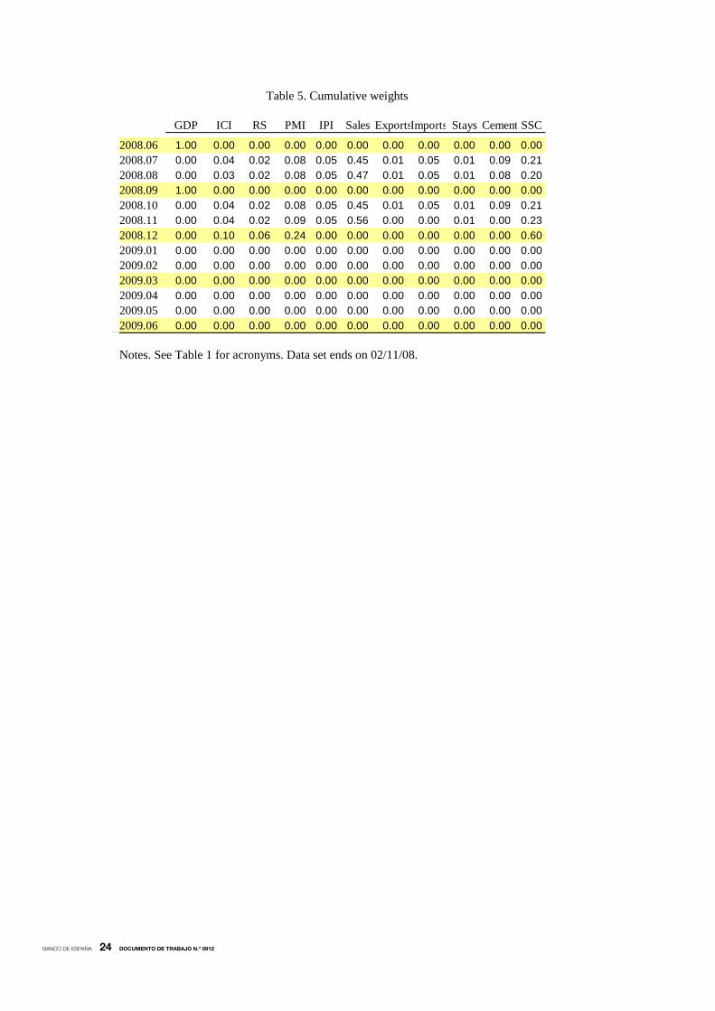
One interesting output of dynamic factor models estimates are the weights or

cumulative impact of each indicator to forecast GDP growth. The weights (standardized

to sum 1) of the indicators in forecasting GDP growth are shown in Table 5. According to the

characteristic of the model, rows labeled as 2008.06 and 2008.09 reveal that, when GDP is

published, the cumulative forecast weights of all the indicators on GDP forecasts are zero

since the published data is a sufficient statistic for the actual figure and its cumulative forecast

weight is one. The series only have weights different from zero during the periods in which the

indicators are available but the corresponding GDP second is not. There are no data referred

to periods after 2008.12 which implies that weights are zero since that date.

Table 4 can also be used to show that ignoring the timely advantages of some

indicators may lead to diminish their role in factor analysis. Recall that IPI was the indicator

with higher factor loading. However, when some indicators are available but IPI is not, as in

the case of the row labeled as 2008.12, the indicators that contribute in a higher scale to

form GDP forecasts are Social Security Contributors (weight of 0.60), and to less extent

the Production Manufacture Index (weight of 0.24). When all the indicators are available

(row 2008.10), Sales has the largest cumulative weight (0.45) in forecasting GDP.

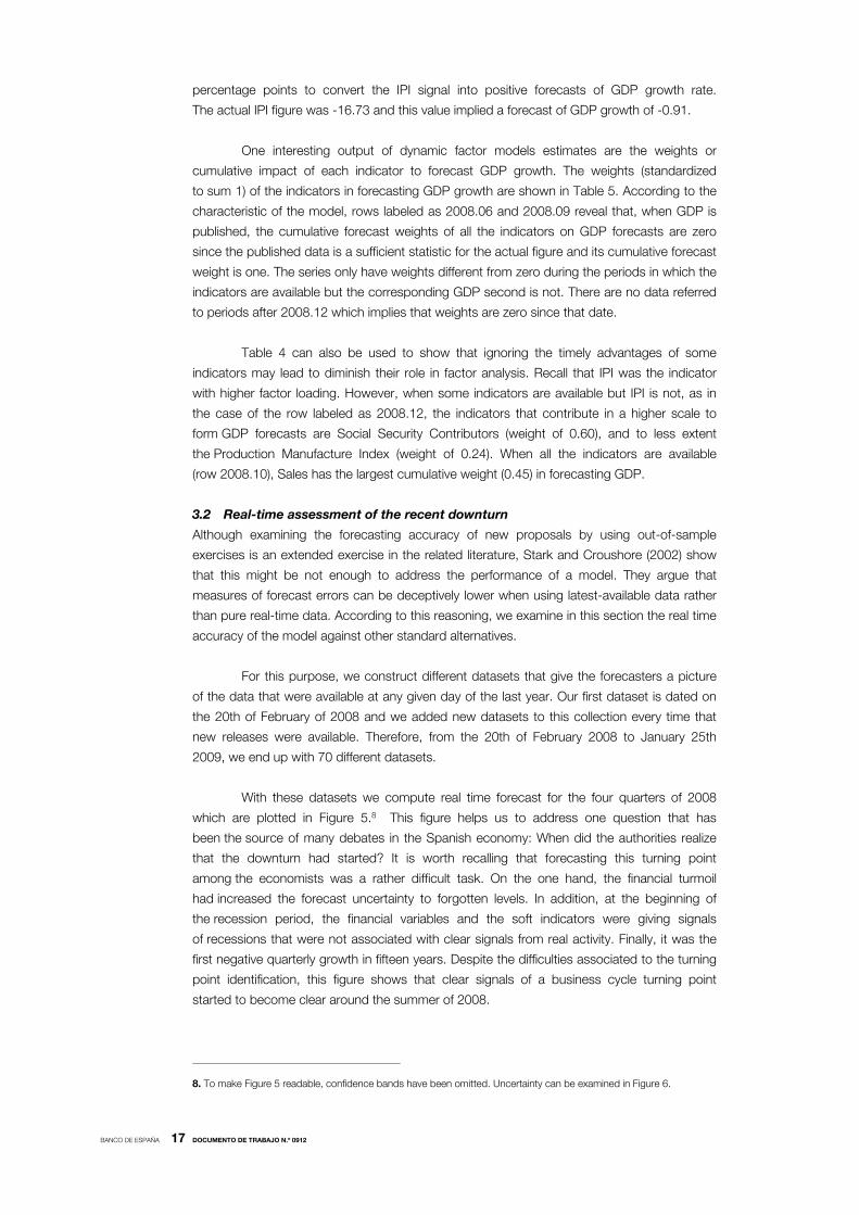
3.2 Real-time assessment of the recent downturn

Although examining the forecasting accuracy of new proposals by using out-of-sample

exercises is an extended exercise in the related literature, Stark and Croushore (2002) show

that this might be not enough to address the performance of a model. They argue that

measures of forecast errors can be deceptively lower when using latest-available data rather

than pure real-time data. According to this reasoning, we examine in this section the real time

accuracy of the model against other standard alternatives.

For this purpose, we construct different datasets that give the forecasters a picture

of the data that were available at any given day of the last year. Our first dataset is dated on

the 20th of February of 2008 and we added new datasets to this collection every time that

new releases were available. Therefore, from the 20th of February 2008 to January 25th

2009, we end up with 70 different datasets.

With these datasets we compute real time forecast for the four quarters of 2008

which are plotted in Figure 5.8 This figure helps us to address one question that has

been the source of many debates in the Spanish economy: When did the authorities realize

that the downturn had started? It is worth recalling that forecasting this turning point

among the economists was a rather difficult task. On the one hand, the financial turmoil

had increased the forecast uncertainty to forgotten levels. In addition, at the beginning of

the recession period, the financial variables and the soft indicators were giving signals

of recessions that were not associated with clear signals from real activity. Finally, it was the

first negative quarterly growth in fifteen years. Despite the difficulties associated to the turning

point identification, this figure shows that clear signals of a business cycle turning point

started to become clear around the summer of 2008.

8. To make Figure 5 readable, confidence bands have been omitted. Uncertainty can be examined in Figure 6.


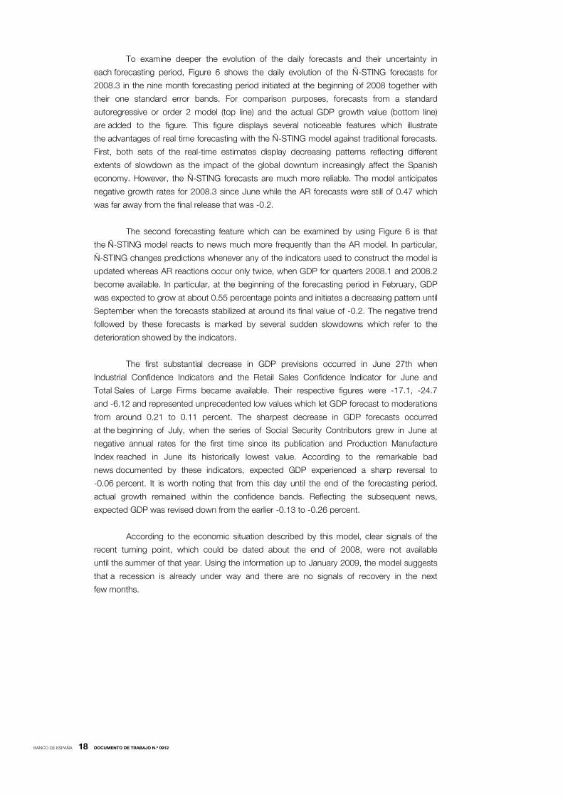
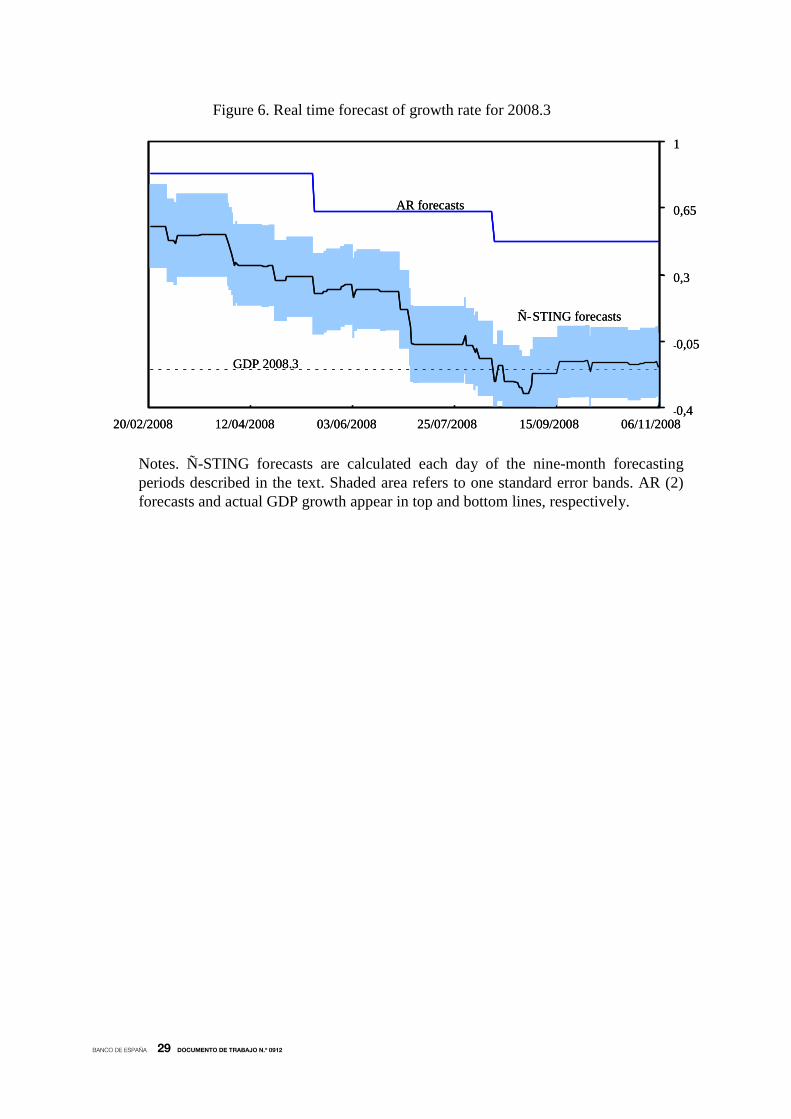
To examine deeper the evolution of the daily forecasts and their uncertainty in

each forecasting period, Figure 6 shows the daily evolution of the Ñ-STING forecasts for

2008.3 in the nine month forecasting period initiated at the beginning of 2008 together with

their one standard error bands. For comparison purposes, forecasts from a standard

autoregressive or order 2 model (top line) and the actual GDP growth value (bottom line)

are added to the figure. This figure displays several noticeable features which illustrate

the advantages of real time forecasting with the Ñ-STING model against traditional forecasts.

First, both sets of the real-time estimates display decreasing patterns reflecting different

extents of slowdown as the impact of the global downturn increasingly affect the Spanish

economy. However, the Ñ-STING forecasts are much more reliable. The model anticipates

negative growth rates for 2008.3 since June while the AR forecasts were still of 0.47 which

was far away from the final release that was -0.2.

The second forecasting feature which can be examined by using Figure 6 is that

the Ñ-STING model reacts to news much more frequently than the AR model. In particular,

Ñ-STING changes predictions whenever any of the indicators used to construct the model is

updated whereas AR reactions occur only twice, when GDP for quarters 2008.1 and 2008.2

become available. In particular, at the beginning of the forecasting period in February, GDP

was expected to grow at about 0.55 percentage points and initiates a decreasing pattern until

September when the forecasts stabilized at around its final value of -0.2. The negative trend

followed by these forecasts is marked by several sudden slowdowns which refer to the

deterioration showed by the indicators.

The first substantial decrease in GDP previsions occurred in June 27th when

Industrial Confidence Indicators and the Retail Sales Confidence Indicator for June and

Total Sales of Large Firms became available. Their respective figures were -17.1, -24.7

and -6.12 and represented unprecedented low values which let GDP forecast to moderations

from around 0.21 to 0.11 percent. The sharpest decrease in GDP forecasts occurred

at the beginning of July, when the series of Social Security Contributors grew in June at

negative annual rates for the first time since its publication and Production Manufacture

Index reached in June its historically lowest value. According to the remarkable bad

news documented by these indicators, expected GDP experienced a sharp reversal to

-0.06 percent. It is worth noting that from this day until the end of the forecasting period,

actual growth remained within the confidence bands. Reflecting the subsequent news,

expected GDP was revised down from the earlier -0.13 to -0.26 percent.

According to the economic situation described by this model, clear signals of the

recent turning point, which could be dated about the end of 2008, were not available

until the summer of that year. Using the information up to January 2009, the model suggests

that a recession is already under way and there are no signals of recovery in the next

few months.


4 Conclusion

In this paper, we provide a concrete mathematical framework within which tracking the

short term evolution of GDP growth rate in Spain. We think that this a serious attempt

to construct a model to forecast GDP growth by dealing with all the problems which

characterize the real time forecasting for the Spanish economy. The method is based on

small scale dynamic factor models which and allow the user to evaluate the impact of several

monthly relevant indicators in quarterly growth forecasts.

One output of the dynamic factor model proposed in the paper is the factor itself.

We provide evidence to consider that the factor can be considered as a good indicator of the

Spanish economic developments in the last two decades. In addition, the model has been

proved in real time forecasting by using pure real-time databases which contain the

information sets that were available at the time of the forecasts. We obtain that the model was

able to anticipate the sudden and sharp recent downturn. For these reasons, we consider

that the model can be useful to construct accurate forecasts of the ongoing Spanish

economic developments.


REFERENCES

ALVAREZ-ARANDA, R., M. CAMACHO and G. PEREZ-QUIROS (2009). Comparison of two estimators for factor models

based on large and small cross section, mimeo.

ANGELINI, E., G. CAMBA-MENDEZ, D. GIANNONE, L. REICHLIN and G. RÜNSTLER (2008). Short-term Forecasts of

Euro Area GDP Growth, CEPR Discussion Paper 6746.

ARUOBA, B., and F. DIEBOLD (2009). Updates on ADS Index Calculation. Available at

http://www.philadelphiafed.org/research-and-data/real-time-center/business-conditions-index/extensions.pdf

ARUOBA, B., F. DIEBOLD and C. SCOTTI (2009). “Real-Time Measurement of Business Conditions”, Journal of

Business and Economic Statistics, in press.

BAI, J., and S. NG (2008). “Forecasting economic time series using targeted predictors”, Journal of Econometrics, 148

pp. 304-317.

BANBURA, M., and G. RÜNSTLER (2007). A look into the factor model black box - publication lags and the role of hard

and soft data in forecasting GDP, ECB Working Paper 751.

BOIVIN, J., and S. NG (2006). “Are more data always better for factor analysis?”, Journal of Econometrics, 132,

pp. 169-194.

CAMACHO, M., and G. PEREZ-QUIROS (2008). Introducing the Euro-STING: Short Term INdicator of Euro Area

Growth, Banco de España Working Paper 0807.

CAMACHO, M., and I. SANCHO (2003). “Spanish diffusion indexes”, Spanish Economic Review, 5, pp. 173-203.

FRALE, C., M. MARCELLINO, G. L. MAZZI and T. PROIETTI (2008). A monthly indicator of the Euro area GDP, CEPR

Discussion Paper 7007.

HAMILTON, J. (1994). “State-space models”, Handbook of Econometrics, Vol. 4, edited by R. Engle and D. McFadden,

North-Holland.

MARIANO, R., and Y. MURASAWA (2003). “A new coincident index of business cycles based on monthly and quarterly

series”, Journal of Applied Econometrics, 18, pp. 427-443.

PROIETTI, T., and F. MOAURO (2006). “Dynamic Factor Analysis with Non Linear Temporal Aggregation Constraints”,

Applied Statistics, 55, pp. 281-300.

STARK, T., and D. CROUSHORE (2002). “Forecasting with a Real-Time Data Set for Macroeconomists”, Journal of

Macroeconomics, 24, pp. 507-531.

STOCK, J., and M. WATSON (1991). “A probability model of the coincident economic indicators”, in Kajal Lahiri and

Geoffrey Moore (Eds.), Leading economic indicators, new approaches and forecasting records, Cambridge University

Press, Cambridge.


Appendix

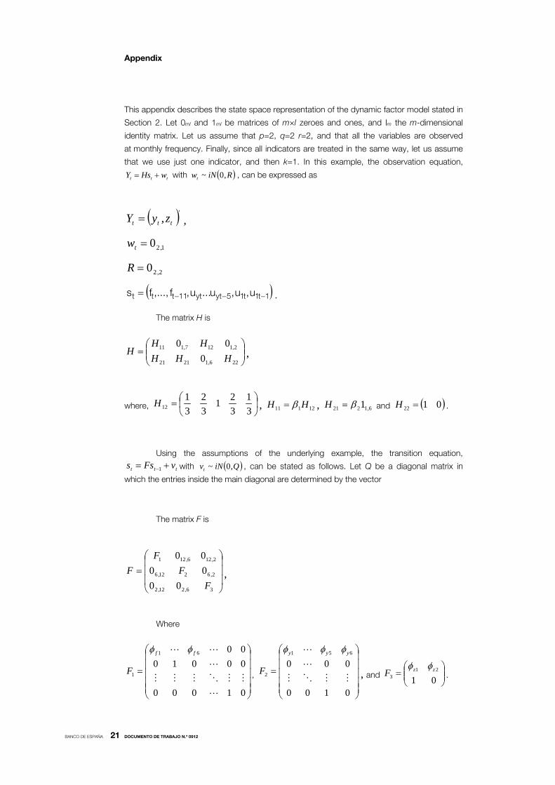
This appendix describes the state space representation of the dynamic factor model stated in

Section 2. Let 0ml and 1ml be matrices of m×l zeroes and ones, and Im the m-dimensional

identity matrix. Let us assume that p=2, q=2 r=2, and that all the variables are observed

at monthly frequency. Finally, since all indicators are treated in the same way, let us assume

that we use just one indicator, and then k=1. In this example, the observation equation,

ttt wHsY += with ( )R,iN~wt 0 , can be expressed as

( )'ttt z,yY = ,

120 ,tw =

220 ,R =

( )1t1t15ytyt11ttt u,u,u...u,f,...,fs −−−= .

The matrix H is

⎟⎟⎠

⎞⎜⎜⎝

⎛=

22612121

21127111

000HHH

HHH

,

,,,

where, ⎟⎠⎞

⎜⎝⎛=

31

321

32

31

12H , 12111 HH β= , 61221 1 ,H β= and ( )0122 =H .

Using the assumptions of the underlying example, the transition equation,

ttt vFss += −1 with ( )Q,iN~vt 0 , can be stated as follows. Let Q be a diagonal matrix in

which the entries inside the main diagonal are determined by the vector

The matrix F is

⎟⎟⎟

⎠

⎞

⎜⎜⎜

⎝

⎛=

362122

262126

2126121

000000

FF

FF

,,

,,

,,

,

Where

⎟⎟⎟⎟⎟

⎠

⎞

⎜⎜⎜⎜⎜

⎝

⎛

=

01000

000100061

1

L

MMOMMM

L

LL ff

F

φφ

, ⎟⎟⎟⎟⎟

⎠

⎞

⎜⎜⎜⎜⎜

⎝

⎛

=

0100

000651

2MMOM

L

L yyy

F

φφφ

, and ⎟⎟⎠

⎞⎜⎜⎝

⎛=

0121

3zzF

φφ.


Table 1. Data description

Indicators Selected for the Ñ-Sting Model:

VariablePeriodicity/Type of

IndicatorSample Reporting Lags

GDP growth Quarterly/Hard 1992.1 -2008.4 +45 days

Industrial ProductionIndex (excl.. energy)

Monthly/Hard 1993.01-2008.11 +35days

Total Sales of LargeFirms

Monthly/Hard 1996.01-2008.11 +32 days

Social SecurityContributors

Monthly/Hard 1996.01-2008.12 0

Retail Sales ConfidenceIndicator

Monthly/Soft 1990.01-2008.12 0

PMI Services Monthly/Soft 1999.08-2008.12 +2 days

Industrial ConfidenceIndicator

Monthly/Soft 1990.01-2008.12 0

Imports Monthly/Hard 1992.01-2008.10 +50days

Exports Monthly/Hard 1992.01-2008.10 +50days

Overnight Stays Monthly/Hard 1991.01-2008.11 +23 days

Cement Consumption Monthly/Hard 1992.01-2008.10 Not a fix date

Notes. Soft indicators are based on surveys while hard indicators are based on economicactivity.


Table 2. Data set available on the day of the forecast

GDP ICI RS PMI IPI Sales Exports Imports Stays Cement SSC2008.06 0.15 -17.10 -24.70 36.70 -10.26 -9.67 -4.75 -4.22 -2.15 -32.73 -0.072008.07 na -16.40 -25.60 37.10 -5.31 -6.25 6.65 -2.81 0.88 -26.50 -0.522008.08 na -17.50 -35.40 39.00 -8.43 -6.58 2.75 -2.10 -1.33 -24.32 -0.852008.09 -0.24 -22.10 -32.90 36.10 -10.27 -8.50 8.50 -4.39 -1.84 -30.06 -1.482008.10 na -27.20 -29.80 32.20 -13.79 -11.32 0.33 -12.34 -4.54 -33.65 -2.412008.11 na -32.60 -26.20 28.20 -16.73 -13.21 na na -10.71 na -3.432008.12 na -37.60 -33.90 32.10 na na na na na na -4.322009.01 na na na na na na na na na na na2009.02 na na na na na na na na na na na2009.03 na na na na na na na na na na na2009.04 na na na na na na na na na na na2009.05 na na na na na na na na na na na2009.06 na na na na na na na na na na na

Notes. See Table 1 for acronyms. Figures labelled as “na” refer to either missing data ordata that are not available on the day of the forecast.

Table 3. Factor loadings

GDP ICI RS PMI IPI Sales Exports Imports Stays Cement SSC0.13 0.05 0.03 0.05 0.07 0.06 0.01 0.04 0.02 0.05 0.06

(0.04) (0.01) (0.01) (0.02) (0.02) (0.02) (0.01) (0.01) (0.01) (0.02) (0.02)

Notes. See Table 1 for acronyms. Standard errors are in parentheses. Data set ends inDecember 2008.

Table 4. Model-based forecasts

Panel A Panel B

Series 2008.4 2009.1 2009.2 Series Next MonthICI -40.32

GDP -0.92 -0.91 -0.80 RS -33.79(0.19) (0.22) (0.25) PMI 29.47

IPI -18.46Sales -14.95Exports 3.12Imports -11.77Stays -8.77Cement -36.05SSC -4.78

Notes. See Table 1 for acronyms. Standard errors are in parentheses. Data set ends onDecember 2008.


Table 5. Cumulative weights

GDP ICI RS PMI IPI Sales ExportsImports Stays Cement SSC

2008.06 1.00 0.00 0.00 0.00 0.00 0.00 0.00 0.00 0.00 0.00 0.002008.07 0.00 0.04 0.02 0.08 0.05 0.45 0.01 0.05 0.01 0.09 0.212008.08 0.00 0.03 0.02 0.08 0.05 0.47 0.01 0.05 0.01 0.08 0.202008.09 1.00 0.00 0.00 0.00 0.00 0.00 0.00 0.00 0.00 0.00 0.002008.10 0.00 0.04 0.02 0.08 0.05 0.45 0.01 0.05 0.01 0.09 0.212008.11 0.00 0.04 0.02 0.09 0.05 0.56 0.00 0.00 0.01 0.00 0.232008.12 0.00 0.10 0.06 0.24 0.00 0.00 0.00 0.00 0.00 0.00 0.602009.01 0.00 0.00 0.00 0.00 0.00 0.00 0.00 0.00 0.00 0.00 0.002009.02 0.00 0.00 0.00 0.00 0.00 0.00 0.00 0.00 0.00 0.00 0.002009.03 0.00 0.00 0.00 0.00 0.00 0.00 0.00 0.00 0.00 0.00 0.002009.04 0.00 0.00 0.00 0.00 0.00 0.00 0.00 0.00 0.00 0.00 0.002009.05 0.00 0.00 0.00 0.00 0.00 0.00 0.00 0.00 0.00 0.00 0.002009.06 0.00 0.00 0.00 0.00 0.00 0.00 0.00 0.00 0.00 0.00 0.00

Notes. See Table 1 for acronyms. Data set ends on 02/11/08.


Figure 1. Time series used in the model

-1.5

-0.5

0.5

1.5

92.1 94.1 96.1 98.1 00.1 02.1 04.1 06.1 08.1

Sample 92.1-08.3

Sample 99.08-08.12

GDP growth rate

Production Manufacture Index

Industrial Production Total Sales of Large Firms

Sample 93.01-08.11 Sample 95.01-08.11

Sample 90.01-08.12

-50

-30

-10

10

90.01 92.08 95.03 97.10 00.05 02.12 05.07 08.02

Retail Sales Index

30

40

50

60

70

90.01 92.05 94.09 97.01 99.05 01.09 04.01 06.05 08.09

-15

0

15

90.01 92.05 94.09 97.01 99.05 01.09 04.01 06.05 08.09-15

0

15

90.01 92.05 94.09 97.01 99.05 01.09 04.01 06.05 08.09

-50

-30

-10

10

90.01 92.08 95.03 97.10 00.05 02.12 05.07 08.02

Industrial Confident Indicator

Sample 90.01-08.12


Figure 1. Time series used in the model (continued)

Exports

Sample 92.01-08.10

-10

10

30

90.01 92.05 94.09 97.01 99.05 01.09 04.01 06.05 08.09

Imports

-20

0

20

40

90.01 92.08 95.03 97.10 00.05 02.12 05.07 08.02

Imports

-20

0

20

40

90.01 92.08 95.03 97.10 00.05 02.12 05.07 08.02

Sample 92.01-08.10

Imports

-20

0

20

40

90.01 92.05 94.09 97.01 99.05 01.09 04.01 06.05 08.09

Sample 91.01-08.11

Overnight Stays

-20

0

20

40

90.01 92.05 94.09 97.01 99.05 01.09 04.01 06.05 08.09

Sample 92.01-08.10

Apparent Consumption of Cement

-35

-15

5

25

90.01 92.08 95.03 97.10 00.05 02.12 05.07 08.02

Sample 96.01-08.12

Social Security Contributions

-5

0

5

90.01 92.08 95.03 97.10 00.05 02.12 05.07 08.02

Notes. GDP is in quarterly growth rates. Soft indicators are in annual differences. Hard indicators are in annual growth rates.


Figure 2. Common factor and Indicador Sintético de Actividad

Notes. The factor (bottom line) is estimated from 91.01 to 09.06 with information in December 2008. Top line refers to annual growth rates of Indice Sintético de Actividad. Dotted line refers to the average value.

-12

-9

-6

-3

0

3

6

90.01 92.10 95.07 98.04 01.01 03.10 06.07 09.04

Figure 3. GDP second growth rate: actual and estimates

Notes. GDP growth rates are estimated from 91.01 to 09.06 with information on December 2008. Dots over this line refer to actual data (third month of each quarter; last one in 2008.3). Dotted line refers to the average value.

-1.8

-1

-0.2

0.6

1.4

90.01 92.11 95.09 98.07 01.05 04.03 07.01


Figure 4. GDP forecast in 2009.1 and IPI potential releases

Notes. Potential releases of IPI in annual growth rates and their associated expected GDP growth rate for 2009.1. Actual IPI was -16.73 which refer to an expected growth rate of -0.91.

-1.2

-0.9

-0.6

-0.3

0

-30 -10 10 30

Potential IPI realizations

Expe

cted

GDP

grow

th ra

te

-0.91

-16.73-1.2

-0.9

-0.6

-0.3

0

-30 -10 10 30

Potential IPI realizations

Expe

cted

GDP

grow

th ra

te

-0.91

-16.73

-0.91

-16.73

Figure 5. Real time growth rates forecasts for 2008Q1, 2008Q2, 2008Q3 and 2008Q420/02/2008 – 25/01/2009

-1,2

-0,8

-0,4

0

0,4

0,8

20/02/2008 31/03/2008 10/05/2008 19/06/2008 29/07/2008 07/09/2008 17/10/2008 26/11/2008 05/01/2009

2008Q1 2008Q2 2008Q3 2008Q4 zero lineGDPQ1 GDPQ2 GDPQ3 GDPQ4

Notes. The figure plots real time forecast of growth rates of GDP and its realization. For example, the green thick line shows the forecast for the fourth quarter of GDP from the first day in which the model produces the forecasts. The thin green horizontal line is the realization.


Notes. Ñ-STING forecasts are calculated each day of the nine-month forecasting periods described in the text. Shaded area refers to one standard error bands. AR (2) forecasts and actual GDP growth appear in top and bottom lines, respectively.

Figure 6. Real time forecast of growth rate for 2008.3

AR forecasts

Ñ-STING forecasts

GDP 2008.3

20/02/2008 12/04/2008 03/06/2008 25/07/2008 15/09/2008 06/11/2008-0,4

-0,05

0,3

0,65

1

AR forecasts

Ñ-STING forecasts

GDP 2008.3

20/02/2008 12/04/2008 03/06/2008 25/07/2008 15/09/2008 06/11/2008-0,4

-0,05

0,3

0,65

1

BANCO DE ESPAÑA PUBLICATIONS

WORKING PAPERS1

0801 ENRIQUE BENITO: Size, growth and bank dynamics.

0802 RICARDO GIMENO AND JOSÉ MANUEL MARQUÉS: Uncertainty and the price of risk in a nominal convergence process.

0803 ISABEL ARGIMÓN AND PABLO HERNÁNDEZ DE COS: Los determinantes de los saldos presupuestarios de las

Comunidades Autónomas.

0804 OLYMPIA BOVER: Wealth inequality and household structure: US vs. Spain.

0805 JAVIER ANDRÉS, J. DAVID LÓPEZ-SALIDO AND EDWARD NELSON: Money and the natural rate of interest:

structural estimates for the United States and the euro area.

0806 CARLOS THOMAS: Search frictions, real rigidities and inflation dynamics.

0807 MAXIMO CAMACHO AND GABRIEL PEREZ-QUIROS: Introducing the EURO-STING: Short Term INdicator of

Euro Area Growth.

0808 RUBÉN SEGURA-CAYUELA AND JOSEP M. VILARRUBIA: The effect of foreign service on trade volumes and

trade partners.

0809 AITOR ERCE: A structural model of sovereign debt issuance: assessing the role of financial factors.

0810 ALICIA GARCÍA-HERRERO AND JUAN M. RUIZ: Do trade and financial linkages foster business cycle

synchronization in a small economy?

0811 RUBÉN SEGURA-CAYUELA AND JOSEP M. VILARRUBIA: Uncertainty and entry into export markets.

0812 CARMEN BROTO AND ESTHER RUIZ: Testing for conditional heteroscedasticity in the components of inflation.

0813 JUAN J. DOLADO, MARCEL JANSEN AND JUAN F. JIMENO: On the job search in a model with heterogeneous

jobs and workers.

0814 SAMUEL BENTOLILA, JUAN J. DOLADO AND JUAN F. JIMENO: Does immigration affect the Phillips curve?

Some evidence for Spain.

0815 ÓSCAR J. ARCE AND J. DAVID LÓPEZ-SALIDO: Housing bubbles.

0816 GABRIEL JIMÉNEZ, VICENTE SALAS-FUMÁS AND JESÚS SAURINA: Organizational distance and use of

collateral for business loans.

0817 CARMEN BROTO, JAVIER DÍAZ-CASSOU AND AITOR ERCE-DOMÍNGUEZ: Measuring and explaining the

volatility of capital flows towards emerging countries.

0818 CARLOS THOMAS AND FRANCESCO ZANETTI: Labor market reform and price stability: an application to the

Euro Area.

0819 DAVID G. MAYES, MARÍA J. NIETO AND LARRY D. WALL: Multiple safety net regulators and agency problems

in the EU: Is Prompt Corrective Action partly the solution?

0820 CARMEN MARTÍNEZ-CARRASCAL AND ANNALISA FERRANDO: The impact of financial position on investment:

an analysis for non-financial corporations in the euro area.

0821 GABRIEL JIMÉNEZ, JOSÉ A. LÓPEZ AND JESÚS SAURINA: Empirical analysis of corporate credit lines.

0822 RAMÓN MARÍA-DOLORES: Exchange rate pass-through in new Member States and candidate countries of the EU.

0823 IGNACIO HERNANDO, MARÍA J. NIETO AND LARRY D. WALL: Determinants of domestic and cross-border bank

acquisitions in the European Union.

0824 JAMES COSTAIN AND ANTÓN NÁKOV: Price adjustments in a general model of state-dependent pricing.

0825 ALFREDO MARTÍN-OLIVER, VICENTE SALAS-FUMÁS AND JESÚS SAURINA: Search cost and price dispersion in

vertically related markets: the case of bank loans and deposits.

0826 CARMEN BROTO: Inflation targeting in Latin America: Empirical analysis using GARCH models.

0827 RAMÓN MARÍA-DOLORES AND JESÚS VAZQUEZ: Term structure and the estimated monetary policy rule in the

eurozone.

0828 MICHIEL VAN LEUVENSTEIJN, CHRISTOFFER KOK SØRENSEN, JACOB A. BIKKER AND ADRIAN VAN RIXTEL:

Impact of bank competition on the interest rate pass-through in the euro area.

0829 CRISTINA BARCELÓ: The impact of alternative imputation methods on the measurement of income and wealth:

Evidence from the Spanish survey of household finances.

0830 JAVIER ANDRÉS AND ÓSCAR ARCE: Banking competition, housing prices and macroeconomic stability.

0831 JAMES COSTAIN AND ANTÓN NÁKOV: Dynamics of the price distribution in a general model of state-dependent

pricing.

1. Previously published Working Papers are listed in the Banco de España publications catalogue.

0832 JUAN A. ROJAS: Social Security reform with imperfect substitution between less and more experienced workers.

0833 GABRIEL JIMÉNEZ, STEVEN ONGENA, JOSÉ LUIS PEYDRÓ AND JESÚS SAURINA: Hazardous times for monetary

policy: What do twenty-three million bank loans say about the effects of monetary policy on credit risk-taking?

0834 ENRIQUE ALBEROLA AND JOSÉ MARÍA SERENA: Sovereign external assets and the resilience of global imbalances.

0835 AITOR LACUESTA, SERGIO PUENTE AND PILAR CUADRADO: Omitted variables in the measure of a labour quality

index: the case of Spain.

0836 CHIARA COLUZZI, ANNALISA FERRANDO AND CARMEN MARTÍNEZ-CARRASCAL: Financing obstacles and growth:

An analysis for euro area non-financial corporations. 0837 ÓSCAR ARCE, JOSÉ MANUEL CAMPA AND ÁNGEL GAVILÁN: Asymmetric collateral requirements and output

composition.

0838 ÁNGEL GAVILÁN AND JUAN A. ROJAS: Solving Portfolio Problems with the Smolyak-Parameterized Expectations Algorithm.

0901 PRAVEEN KUJAL AND JUAN RUIZ: International trade policy towards monopoly and oligopoly.

0902 CATIA BATISTA, AITOR LACUESTA AND PEDRO VICENTE: Micro evidence of the brain gain hypothesis: The case of Cape Verde.

0903 MARGARITA RUBIO: Fixed and variable-rate mortgages, business cycles and monetary policy.

0904 MARIO IZQUIERDO, AITOR LACUESTA AND RAQUEL VEGAS: Assimilation of immigrants in Spain: A longitudinal analysis.

0905 ÁNGEL ESTRADA: The mark-ups in the Spanish economy: international comparison and recent evolution.

0906 RICARDO GIMENO AND JOSÉ MANUEL MARQUÉS: Extraction of financial market expectations about inflation and interest rates from a liquid market.

0907 LAURA HOSPIDO: Job changes and individual-job specific wage dynamics.

0908 M.a DE LOS LLANOS MATEA AND JUAN S. MORA: La evolución de la regulación del comercio minorista en España y sus implicaciones macroeconómicas.

0909 JAVIER MENCÍA AND ENRIQUE SENTANA: Multivariate location-scale mixtures of normals and mean-variance-skewness portfolio allocation

0910 ALICIA GARCÍA-HERRERO, SERGIO GAVILÁ AND DANIEL SANTABÁRBARA: What explains the low profitability of Chinese banks?

0911

0912

MENCÍA: Assessing the risk-return trade-off in loans portfolios.

MAXIMO CAMACHO AND GABRIEL PEREZ-QUIROS: Ñ-STING: España Short Term INdicator of Growth.

Unidad de PublicacionesAlcalá, 522; 28027 Madrid

Telephone +34 91 338 6363. Fax +34 91 338 6488e-mail: [email protected]

www.bde.es

Documents

Maximo Camacho and Gabriel Perez-Quiros fileÑ-STING: ESPAÑA SHORT TERM INDICATOR OF GROWTH (*) Maximo Camacho UNIVERSIDAD DE MURCIA Gabriel Perez-Quiros BANCO DE ESPAÑA AND CEPR