Manual Do Simulador

8/12/2019 Manual Do Simulador

http://slidepdf.com/reader/full/manual-do-simulador 1/27

Sim.I.am: A Robot SimulatorCoursera: Control of Mobile Robots

Jean-Pierre de la Croix

Last Updated: February 28, 2014

Contents

1 Introduction 2

1.1 Installation . . . . . . . . . . . . . . . . . . . . . . . . . . . . . . . . . . . . . . . . . . . . 21.2 Requirements . . . . . . . . . . . . . . . . . . . . . . . . . . . . . . . . . . . . . . . . . . . 21.3 Bug Reporting . . . . . . . . . . . . . . . . . . . . . . . . . . . . . . . . . . . . . . . . . . 2

2 Mobile Robot 3

2.1 IR Range Sensors . . . . . . . . . . . . . . . . . . . . . . . . . . . . . . . . . . . . . . . . . 32.2 Differential Wheel Drive . . . . . . . . . . . . . . . . . . . . . . . . . . . . . . . . . . . . . 42.3 Wheel Encoders . . . . . . . . . . . . . . . . . . . . . . . . . . . . . . . . . . . . . . . . . . 5

3 Simulator 6

4 Programming Assignments 7

4.1 Week 1 . . . . . . . . . . . . . . . . . . . . . . . . . . . . . . . . . . . . . . . . . . . . . . . 74.2 Week 2 . . . . . . . . . . . . . . . . . . . . . . . . . . . . . . . . . . . . . . . . . . . . . . . 84.3 Week 3 . . . . . . . . . . . . . . . . . . . . . . . . . . . . . . . . . . . . . . . . . . . . . . . 114.4 Week 4 . . . . . . . . . . . . . . . . . . . . . . . . . . . . . . . . . . . . . . . . . . . . . . . 154.5 Week 5 . . . . . . . . . . . . . . . . . . . . . . . . . . . . . . . . . . . . . . . . . . . . . . . 18

4.6 Week 6 . . . . . . . . . . . . . . . . . . . . . . . . . . . . . . . . . . . . . . . . . . . . . . . 234.7 Week 7 . . . . . . . . . . . . . . . . . . . . . . . . . . . . . . . . . . . . . . . . . . . . . . . 26

1



1 Introduction

This manual is going to be your resource for using the simulator with the programming assignmentsfeatured in the Coursera course, Control of Mobile Robots (and included at the end of this manual). Itwill be updated from time to time whenever new features are added to the simulator or any correctionsto the course material are made.

1.1 Installation

Download simiam-coursera-week-X.zip (where X is the corresponding week number for the assignment)from the course page on Coursera under Programming Assignments . Make sure to download a new copyof the simulator before you start a new week’s programming assignment, or whenever an announcementis made that a new version is available. It is important to stay up-to-date, since new versions may containimportant bug fixes or features required for the programming assignment.

Unzip the .zip file to any directory.

1.2 Requirements

You will need a reasonably modern computer to run the robot simulator. While the simulator will run

on hardware older than a Pentium 4, it will probably be a very slow experience. You will also need acopy of MATLAB.

Thanks to support from MathWorks, a license for MATLAB and all required toolboxes is availableto all students for the duration of the course. Check the Getting Started with MATLAB section underProgramming Assignments on the course page for detailed instructions on how to download and installMATLAB on your computer.

1.3 Bug Reporting

If you run into a bug (issue) with the simulator, please create a post on the discussion forums in theProgramming Assignments section. Make sure to leave a detailed description of the bug. Any questionsor issues with MATLAB itself should be posted on the discussion forums in the MATLAB section.

2

https://class.coursera.org/conrob-002/wiki/ProgrammingAssignments



https://class.coursera.org/conrob-002/forum/list?forum_id=3








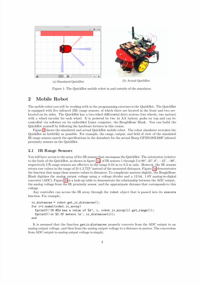
(a) Simulated QuickBot (b) Actual QuickBot

Figure 1: The QuickBot mobile robot in and outside of the simulator.

2 Mobile RobotThe mobile robot you will be working with in the programming exercises is the QuickBot. The QuickBotis equipped with five infrared (IR) range sensors, of which three are located in the front and two arelocated on its sides. The QuickBot has a two-wheel differential drive system (two wheels, two motors)with a wheel encoder for each wheel. It is powered by two 4x AA battery packs on top and can becontrolled via software on its embedded Linux computer, the BeagleBone Black. You can build theQuickBot yourself by following the hardware lectures in this course.

Figure 2 shows the simulated and actual QuickBot mobile robot. The robot simulator recreates theQuickBot as faithfully as possible. For example, the range, output, and field of view of the simulatedIR range sensors match the specifications in the datasheet for the actual Sharp GP2D120XJ00F infraredproximity sensors on the QuickBot.

2.1 IR Range Sensors

You will have access to the array of five IR sensors that encompass the QuickBot. The orientation (relativeto the body of the QuickBot, as shown in figure 1a) of IR sensors 1 through 5 is 90◦, 45◦, 0◦, −45◦,−90◦,respectively.I R range sensors are effective in the range 0.04 m to 0.3 m only. However, the IR sensorsreturn raw values in the range of [0.4, 2.75]V instead of the measured distances. Figure 2a demonstratesthe function that maps these sensors values to distances. To complicate matters slightly, the BeagleBoneBlack digitizes the analog output voltage using a voltage divider and a 12-bit, 1.8V analog-to-digitalconverter (ADC). Figure 2b is a look-up table to demonstrate the relationship between the ADC output,the analog voltage from the IR proximity sensor, and the approximate distance that corresponds to thisvoltage.

Any controller can access the IR array through the robot object that is passed into its execute

function. For example,

ir_distances = robot.get_ir_distances();

for i=1:numel(robot.ir_array)

fprintf(’IR #%d has a value of %d’, i, robot.ir_array(i).get_range());

fprintf(’or %0.3f meters.\n’, ir_distances(i));

end

It is assumed that the function get ir distances properly converts from the ADC output to ananalog output voltage, and then from the analog output voltage to a distance in meters. The conversionfrom ADC output to analog output voltage is simply,

3



0 0.05 0.1 0.15 0.2 0.25 0.3 0.350

0.5

1

1.5

2

2.5

3

Distance (m)

V o l t a g e

( V )

(a) Analog voltage output when an object is be-tween 0.04m and 0.3m in the IR proximity sensor’sfield of view.

Distance (m) Voltage (V) ADC Out0.04 2.750 9170.05 2.350 7830.06 2.050 6830.07 1.750 583

0.08 1.550 5170.09 1.400 4670.10 1.275 4250.12 1.075 3580.14 0.925 3080.16 0.805 2680.18 0.725 2420.20 0.650 2170.25 0.500 1670.30 0.400 133

(b) A look-up table for interpolating a distance (m)

from the analog (and digital) output voltages.

Figure 2: A graph and a table illustrating the relationship between the distance of an object within thefield of view of an infrared proximity sensor and the analog (and digital) ouptut voltage of the sensor.

V ADC =

1000 · V analog

3

NOTE: For Week 2, the simulator uses a different voltage divider on the ADC; therefore,

V ADC = V analog ∗ 1000/2. This has been fixed in subsequent weeks!

Converting from the the analog output voltage to a distance is a little bit more complicated, becausea) the relationships between analog output voltage and distance is not linear, and b) the look-up tableprovides a coarse sample of points on the curve in Figure 2a. MATLAB has a polyfit function to fita curve to the values in the look-up table, and a polyval function to interpolate a point on that fittedcurve. The combination of the these two functions can be use to approximate a distance based on theanalog output voltage. For more information, see Section 4.2.

It is important to note that the IR proximity sensor on the actual QuickBot will be influencedby ambient lighting and other sources of interference. For example, under different ambient lightingconditions, the same analog output voltage may correspond to different distances of an object from theIR proximity sensor. This effect of ambient lighting (and other sources of noise) is not modelled in thesimulator, but will be apparent on the actual hardware.

2.2 Differential Wheel Drive

Since the QuickBot has a differential wheel drive (i.e., is not a unicyle), it has to be controlled by specifyingthe angular velocities of the right and left wheel (vr, vl), instead of the linear and angular velocities of a unicycle (v, ω). These velocities are computed by a transformation from (v, ω) to (vr, v). Recall thatthe dynamics of the unicycle are defined as,

x = vcos(θ)

y = vsin(θ)

θ = ω.

(1)

4



The dynamics of the differential drive are defined as,

x = R

2 (vr + v)cos(θ)

y = R

2 (vr + v)sin(θ)

θ = RL

(vr − v),

(2)

where R is the radius of the wheels and L is the distance between the wheels.The speed of the QuickBot can be set in the following way assuming that the uni to diff function

has been implemented, which transforms (v, ω) to (vr, v):

v = 0.15; % m/s

w = pi/4; % rad/s

% Transform from v,w to v_r,v_l and set the speed of the robot

[vel_r, vel_l] = obj.robot.dynamics.uni_to_diff(robot,v,w);

obj.robot.set_speeds(vel_r, vel_l);

The maximum angular wheel velocity for the QuickBot is approximately 80 RPM or 8.37 rad/s.It is important to note that if the QuickBot is controlled ot move at maximum linear velocity, it isnot possible to achieve any angular velocity, because the angular velocity of the wheel will have beenmaximized. Therefore, there exists a tradeoff between the linear and angular velocity of the QuickBot:the faster the robot should turn, the slower it has to move forward .

2.3 Wheel Encoders

Each of the wheels is outfitted with a wheel encoder that increments or decrements a tick counterdepending on whether the wheel is moving forward or backwards, respectively. Wheel encoders may beused to infer the relative pose of the robot. This inference is called odometry. The relevant informationneeded for odometry is the radius of the wheel (32 .5mm), the distance between the wheels (99.25mm),and the number of ticks per revolution of the wheel (16 ticks/rev). For example,

R = robot.wheel_radius; % radius of the wheel

L = robot.wheel_base_length; % distance between the wheels

tpr = robot.encoders(1).ticks_per_rev; % ticks per revolution for the right wheel

fprintf(’The right wheel has a tick count of %d\n’, robot.encoders(1).state);

fprintf(’The left wheel has a tick count of %d\n’, robot.encoders(2).state);

For more information about odometry, see Section 4.2.

5



3 Simulator

Start the simulator with the launch command in MATLAB from the command window. It is importantthat this command is executed inside the unzipped folder (but not inside any of its subdirectories).

(a) Simulator (b) Submission screen

Figure 3: launch starts the simulator, while submit brings up the submission tool.

Figure 3a is a screenshot of the graphical user interface (GUI) of the simulator. The GUI can becontrolled by the bottom row of buttons. The first button is the Home button and returns you to thehome screen. The second button is the Rewind button and resets the simulation. The third button is thePlay button, which can be used to play and pause the simulation. The set of Zoom buttons or the mousescroll wheel allows you to zoom in and out to get a better view of the simulation. Clicking, holding, andmoving the mouse allows you to pan around the environment. You can click on a robot to follow it as itmoves through the environment.

Figure 3b is a screenshot of the submission screen. Each assignment can be submitted to Courserafor automatic grading and feedback. Start the submission tool by typing submit into the MATLABcommand window. Use your login and password from the Assignments page. Your Coursera login andpassword will not work. Select which parts of the assignments in the list you would like to submit, thenclick Submit to Coursera for Grading . You will receive feedback, either a green checkmark for pass, ora red checkmark for fail. If you receive a red checkmark, check the MATLAB command window for ahelpful message.

6

https://class.coursera.org/conrob-002/assignment/list

https://class.coursera.org/conrob-002/assignment/list



4 Programming Assignments

The following sections serve as a tutorial for getting through the simulator portions of the programmingexercises. Places where you need to either edit or add code is marked off by a set of comments. Forexample,

%% START CODE BLOCK %%[edit or add code here]

%% END CODE BLOCK %%

To start the simulator with the launch command from the command window, it is important thatthis command is executed inside the unzipped folder (but not inside any of its subdirectories).

4.1 Week 1

This week’s exercises will help you learn about MATLAB and robot simulator:

1. Since the assignments in this course involve programming in MATLAB, you should familiarizeyourself with MATLAB (both the environment and the language). Review the resources posted in

the ”Getting Started with MATLAB” section on the Programming Assignments page.

2. Familiarize yourself with the simulator by reading this manual and downloading the robot simulatorposted on the Programming Assignments section on the Coursera page.

7







4.2 Week 2

Start by downloading the robot simulator for this week from the Week 2 programming assignment. Beforeyou can design and test controllers in the simulator, you will need to implement three components of thesimulator:

1. Implement the transformation from unicycle dynamics to differential drive dynamics, i.e. convertfrom (v, ω) to the right and left angular wheel speeds (vr, vl).

In the simulator, (v, ω) corresponds to the variables v and w, while (vr, vl) correspond to thevariables vel r and vel l. The function used by the controllers to convert from unicycle dynamicsto differential drive dynamics is located in +simiam/+robot/+dynamics/DifferentialDrive.m.The function is named uni to diff, and inside of this function you will need to define vel r (vr)and vel l (vl) in terms of v, w, R, and L. R is the radius of a wheel, and L is the distance separatingthe two wheels. Make sure to refer to Section 2.2 on “Differential Wheel Drive” for the dynamics.

2. Implement odometry for the robot, such that as the robot moves around, its pose (x,y,θ) is esti-mated based on how far each of the wheels have turned. Assume that the robot starts at (0,0,0).

The tutorial located at www.orcboard.org/wiki/images/1/1c/OdometryTutorial.pdf covers howodometry is computed. The general idea behind odometry is to use wheel encoders to measure the

distance the wheels have turned over a small period of time, and use this information to approximatethe change in pose of the robot.

The pose of the robot is composed of its position ( x, y) and its orientation θ on a 2 dimensionalplane (note: the video lecture may refer to robot’s orientation as φ). The currently estimatedpose is stored in the variable state estimate, which bundles x (x), y (y), and theta (θ). Therobot updates the estimate of its pose by calling the update odometry function, which is locatedin +simiam/+controller/+quickbot/QBSupervisor.m. This function is called every dt seconds,where dt is 0.033s (or a little more if the simulation is running slower).

% Get wheel encoder ticks from the robot

right_ticks = obj.robot.encoders(1).ticks;

left_ticks = obj.robot.encoders(2).ticks;

% Recall the wheel encoder ticks from the last estimateprev_right_ticks = obj.prev_ticks.right;

prev_left_ticks = obj.prev_ticks.left;

% Previous estimate

[x, y, theta] = obj.state_estimate.unpack();

% Compute odometry here

R = obj.robot.wheel_radius;

L = obj.robot.wheel_base_length;

m_per_tick = (2*pi*R)/obj.robot.encoders(1).ticks_per_rev;

The above code is already provided so that you have all of the information needed to estimate the

change in pose of the robot. right ticks and left ticks are the accumulated wheel encoder ticksof the right and left wheel. prev right ticks and prev left ticks are the wheel encoder ticksof the right and left wheel saved during the last call to update odometry. R is the radius of eachwheel, and L is the distance separating the two wheels. m per tick is a constant that tells youhow many meters a wheel covers with each tick of the wheel encoder. So, if you were to multiply

m per tick by (right ticks-prev right ticks), you would get the distance travelled by the rightwheel since the last estimate.

Once you have computed the change in (x,y,θ) (let us denote the changes as x dt, y dt, andtheta dt) , you need to update the estimate of the pose:

8

https://class.coursera.org/conrob-002/assignment/view?assignment_id=5

http://www.orcboard.org/wiki/images/1/1c/OdometryTutorial.pdf

http://www.orcboard.org/wiki/images/1/1c/OdometryTutorial.pdf

https://class.coursera.org/conrob-002/assignment/view?assignment_id=5



theta_new = theta + theta_d;

x_new = x + x_dt;

y_new = y + y_dt;

3. Read the ”IR Range Sensors” section in the manual and take note of the table in Figure 2b, whichmaps distances (in meters) to raw IR values. Implement code that converts raw IR values todistances (in meters).

To retrieve the distances (in meters) measured by the IR proximity sensor, you will need to imple-ment a conversion from the raw IR values to distances in the get ir distances function locatedin +simiam/+robot/Quickbot.m.

function ir_distances = get_ir_distances(obj)

ir_array_values = obj.ir_array.get_range();

ir_voltages = ir_array_values;

coeff = [];

ir_distances = polyval(coeff, ir_voltages);

end

The variable ir array values is an array of the IR raw values. Divide this array by 500 to computethe ir voltages array. The coeff should be the coefficients returned by

coeff = polyfit(ir_voltages_from_table, ir_distances_from_table, 5);

where the first input argument is an array of IR voltages from the table in Figure 2b and the secondargument is an array of the corresponding distances from the table in Figure 2b. The third argumentspecifies that we will use a fifth-order polynomial to fit to the data. Instead of running this fit everytime, execute the polyfit once in the MATLAB command line, and enter them manually on thethird line, i.e. coeff = [ ... ];. If the coefficients are properly computed, then the last linewill use polyval to convert from IR voltages to distances using a fifth-order polynomial using thecoefficients in coeff.

How to test it all

To test your code, the simulator will is set to run a single P-regulator that will steer the robot to a partic-ular angle (denoted θd or, in code, theta d). This P-regulator is implemented in +simiam/+controller/

GoToAngle.m. If you want to change the linear velocity of the robot, or the angle to which it steers, editthe following two lines in +simiam/+controller/+quickbot/QBSupervisor.m

obj.theta_d = pi/4;

obj.v = 0.1; %m/s

1. To test the transformation from unicycle to differential drive, first set obj.theta d=0. The robotshould drive straight forward. Now, set obj.theta d to positive or negative π

4. If positive, the robot

should start off by turning to its left, if negative it should start off by turning to its right. Note:

If you haven’t implemented odometry yet, the robot will just keep on turning in that direction.2. To test the odometry, first make sure that the transformation from unicycle to differential drive

works correctly. If so, set obj.theta d to some value, for example π4

, and the robot’s P-regulatorshould steer the robot to that angle. You may also want to uncomment the fprintf statement inthe update odometry function to print out the current estimate position to see if it make sense.Remember, the robot starts at (x,y,θ) = (0, 0, 0).

3. To test the IR raw to distances conversion, edit +simiam/+controller/GoToAngle.m and uncom-ment the following section:

9



% for i=1:numel(ir_distances)

% fprintf(’IR %d: %0.3fm\n’, i, ir_distances(i));

% end

This for loop will print out the IR distances. If there are no obstacles (for example, walls) aroundthe robot, these values should be close (if not equal to) 0.3m. Once the robot gets within range of a wall, these values should decrease for some of the IR sensors (depending on which ones can sensethe obstacle). Note: The robot will eventually collide with the wall, because we have not designedan obstacle avoidance controller yet!

10



4.3 Week 3

Start by downloading the new robot simulator for this week from the Week 3 programming assignment.This week you will be implementing the different parts of a PID regulator that steers the robot successfullyto some goal location. This is known as the go-to-goal behavior:

1. Calculate the heading (angle), θg, to the goal location (xg, yg). Let u be the vector from the robotlocated at (x, y) to the goal located at (xg, yg), then θg is the angle u makes with the x-axis (positiveθg is in the counterclockwise direction).

All parts of the PID regulator will be implemented in the file +simiam/+controller/GoToGoal.m.Take note that each of the three parts is commented to help you figure out where to code each part.The vector u can be expressed in terms of its x-component, ux, and its y-component, uy. ux shouldbe assigned to u x and uy to u y in the code. Use these two components and the atan2 function tocompute the angle to the goal, θg (theta g in the code).

2. Calculate the error between θg and the current heading of the robot, θ .

The error e k should represent the error between the heading to the goal theta g and the currentheading of the robot theta. Make sure to use atan2 and/or other functions to keep the errorbetween [−π, π].

3. Calculate the proportional, integral, and derivative terms for the PID regulator that steers therobot to the goal.

As before, the robot will drive at a constant linear velocity v, but it is up to the PID regulator tosteer the robot to the goal, i.e compute the correct angular velocity w. The PID regulator needsthree parts implemented:

(i) The first part is the proportional term e P. It is simply the current error e k. e P is multipliedby the proportional gain obj.Kp when computing w.

(ii) The second part is the integral term e I. The integral needs to be approximated in discretetime using the total accumulated error obj.E k, the current error e k, and the time step dt.e I is multiplied by the integral gain obj.Ki when computing w, and is also saved as obj.E k

for the next time step.(iii) The third part is the derivative term e D. The derivative needs to be approximated in discrete

time using the current error e k, the previous error obj.e k 1, and the the time step dt. e D

is multiplied by the derivative gain obj.Kd when computing w, and the current error e k issaved as the previous error obj.e k 1 for the next time step.

Now, you need to tune your PID gains to get a fast settle time (θ matches θg within 10% in threeseconds or less) and there should be little overshoot (maximum θ should not increase beyond 10%of the reference value θg). What you don’t want to see are the following two graphs when the robottries to reach goal location (xg, yg) = (0,−1):

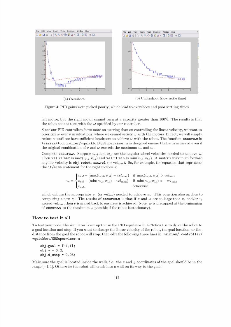
Figure 4b demonstrates undershoot, which could be fixed by increasing the proportional gain oradding some integral gain for better tracking. Picking better gains leads to the graph in Figure 5.

4. Ensure that the robot steers with an angular velocity ω, even if the combination of v and ω exceedsthe maximum angular velocity of the robot’s motors.

This week we’ll tackle the first of two limitations of the motors on the QuickBot. The first limitationis that the robot’s motors have a maximum angular velocity, and the second limitation is that themotors stall at low speeds. We will discuss the latter limitation in a later week and focus ourattention on the first limitation. Suppose that we pick a linear velocity v that requires the motorsto spin at 90% power. Then, we want to change ω from 0 to some value that requires 20% morepower from the right motor, and 20% less power from the left motor. This is not an issue for the

11



(a) Overshoot (b) Undershoot (slow settle time)

Figure 4: PID gains were picked poorly, which lead to overshoot and poor settling times.

left motor, but the right motor cannot turn at a capacity greater than 100%. The results is thatthe robot cannot turn with the ω specified by our controller.

Since our PID controllers focus more on steering than on controlling the linear velocity, we want toprioritize ω over v in situations, where we cannot satisfy ω with the motors. In fact, we will simplyreduce v until we have sufficient headroom to achieve ω with the robot. The function ensure w in+simiam/+controller/+quickbot/QBSupervisor.m is designed ensure that ω is achieved even if the original combination of v and ω exceeds the maximum vr and vl.

Complete ensure w. Suppose vr,d and vl,d are the angular wheel velocities needed to achieve ω.Then vel rl max is max(vr,d, vl,d) and vel rl min is min(vr,d, vl,d). A motor’s maximum forwardangular velocity is obj.robot.max vel (or velmax). So, for example, the equation that representsthe if/else statement for the right motors is:

vr =

vr,d − (max(vr,d, vl,d) − velmax) if max(vr,d, vl,d) > velmax

vr,d − (min(vr,d, vl,d) + velmax) if min(vr,d, vl,d) < −velmax

vr,d, otherwise,

which defines the appropriate vr (or vel r) needed to achieve ω. This equation also applies tocomputing a new vl. The results of ensures w is that if v and ω are so large that vr and/or vlexceed velmax, then v is scaled back to ensure ω is achieved (Note: ω is precapped at the beginngingof ensure w to the maximum ω possible if the robot is stationary).

How to test it all

To test your code, the simulator is set up to use the PID regulator in GoToGoal.m to drive the robot to

a goal location and stop. If you want to change the linear velocity of the robot, the goal location, or thedistance from the goal the robot will stop, then edit the following three lines in +simiam/+controller/

+quickbot/QBSupervisor.m.

obj.goal = [-1,1];

obj.v = 0.2;

obj.d_stop = 0.05;

Make sure the goal is located inside the walls, i.e. the x and y coordinates of the goal should be in therange [−1, 1]. Otherwise the robot will crash into a wall on its way to the goal!

12



Figure 5: Faster settle time and good tracking with little overshoot.

1. To test the heading to the goal, set the goal location to obj.goal = [1,1]. theta g should beapproximately π

4 ≈ 0.785 initially, and as the robot moves forward (since v = 0.1 and ω = 0)

theta g should increase. Check it using a fprintf statment or the plot that pops up. theta g

corresponds to the red dashed line (i.e., it is the reference signal for the PID regulator).

2. Test this part with the implementation of the third part.

3. To test the third part, run the simulator and check if the robot drives to the goal location andstops. In the plot, the blue solid line (theta) should match up with the red dashed line (theta g).You may also use fprintf statements to verify that the robot stops within obj.d stop meters of the goal location.

4. To test the fourth part, set obj.v=10. Then add the following two lines of code after the call toensure w in the execute function of QBSupervisor.m.

[v_limited, w_limited] = obj.robot.dynamics.diff_to_uni(vel_r, vel_l);

fprintf(’(v,w) = (%0.3f,%0.3f), (v_limited,w_limited) = (%0.3f, %0.3f)\n’, ...

outputs.v, outputs.w, v_limited, w_limited);

If ω = ωlimited, then ω is not ensured by ensure w. This function should scale back v , such that itis possible for the robot to turn with the ω output by the controller (unless |ω| > 5.48 rad/s).

How to migrate your solutions from last week.

Here are a few pointers to help you migrate your own solutions from last week to this week’s simulatorcode. You only need to pay attention to this section if you want to use your own solutions, otherwise youcan use what is provided for this week and skip this section.

1. You may overwrite +simiam/+robot/+dynamics/DifferentialDrive.m with your own versionfrom last week.

2. You should not overwrite +simiam/+robot/QuickBot.m with your own version from last week!Many changes were made to this file for this week.

13



3. You should not overwrite +simiam/+controller/+quickbot/QBSupervisor.m! However, to useyour own solution to the odometry, you can replace the provided update odometry function inQBSupervisor.m with your own version from last week.

14



4.4 Week 4

Start by downloading the new robot simulator for this week from the Week 4 programming assignment.This week you will be implementing the different parts of a controller that steers the robot successfullyaway from obstacles to avoid a collision. This is known as the avoid-obstacles behavior. The IR sensorsallow us to measure the distance to obstacles in the environment, but we need to compute the points in

the world to which these distances correspond. Figure 6 illustrates these points with a black cross. The

Figure 6: IR range to point transformation.

strategy for obstacle avoidance that we will use is as follows:

1. Transform the IR distances to points in the world.

2. Compute a vector to each point from the robot, u1, u2, . . . , u9.

3. Weigh each vector according to their importance, α1u1, α2u2, . . . , α9u9. For example, the front andside sensors are typically more important for obstacle avoidance while moving forward.

4. Sum the weighted vectors to form a single vector, uao = α1u1 + . . . + α9u9.

5. Use this vector to compute a heading and steer the robot to this angle.

This strategy will steer the robot in a direction with the most free space (i.e., it is a direction away

from obstacles). For this strategy to work, you will need to implement three crucial parts of the strategyfor the obstacle avoidance behavior:

1. Transform the IR distance (which you converted from the raw IR values in Week 2) measured byeach sensor to a point in the reference frame of the robot.

A point pi that is measured to be di meters away by sensor i can be written as the vector (co-

ordinate) vi =

di

0

in the reference frame of sensor i. We first need to transform this point to

be in the reference frame of the robot. To do this transformation, we need to use the pose (lo-cation and orientation) of the sensor in the reference frame of the robot: (xsi , ysi , θsi) or in code,(x s,y s,theta s). The transformation is defined as:

v

i = R(xsi , ysi , θsi)

vi1

,

15



where R is known as the transformation matrix that applies a translation by (x, y) and a rotationby θ :

R(x,y,θ) =

cos(θ) − sin(θ) x

sin(θ) cos(θ) y0 0 1

,

which you need to implement in the function obj.get transformation matrix.In +simiam/+controller/+AvoidObstacles.m, implement the transformation in the apply sensor

geometry function. The objective is to store the transformed points in ir distances rf, such thatthis matrix has v

1 as its first column, v

2 as its second column, and so on.

2. Transform the point in the robot’s reference frame to the world’s reference frame.

A second transformation is needed to determine where a point pi is located in the world that ismeasured by sensor i. We need to use the pose of the robot, (x,y,θ), to transform the robot fromthe robot’s reference frame to the world’s reference frame. This transformation is defined as:

v

i = R(x,y,θ)v

i

In +simiam/+controller/+AvoidObstacles.m, implement this transformation in the apply sensor

geometry function. The objective is to store the transformed points in ir distances wf, such thatthis matrix has v

1 as its first column, v

2 as its second column, and so on. This matrix now containsthe coordinates of the points illustrated in Figure 6 by the black crosses. Note how these pointsapproximately correspond to the distances measured by each sensor (Note: approximately , becauseof how we converted from raw IR values to meters in Week 2).

3. Use the set of transformed points to compute a vector that points away from the obstacle. Therobot will steer in the direction of this vector and successfully avoid the obstacle.

In the function execute implement parts 2.-4. of the obstacle avoidance strategy.

(i) Compute a vector ui to each point (corresponding to a particular sensor) from the robot. Use apoint’s coordinate from ir distances wf and the robot’s location (x,y) for this computation.

(ii) Pick a weight αi for each vector according to how important you think a particular sensoris for obstacle avoidance. For example, if you were to multiply the vector from the robot topoint i (corresponding to sensor i) by a small value (e.g., 0.1), then sensor i will not impactobstacle avoidance significantly. Set the weights in sensor gains. Note: Make sure to thatthe weights are symmetric with respect to the left and right sides of the robot. Without anyobstacles around, the robot should only steer slightly right (due to a small asymmetry in thehow the IR sensors are mounted on the robot).

(iii) Sum up the weighted vectors, αiui, into a single vector uao.

(iv) Use uao and the pose of the robot to compute a heading that steers the robot away fromobstacles (i.e., in a direction with free space, because the vectors that correspond to directionswith large IR distances will contribute the most to uao).

QuickBot Motor LimitationsLast week we implemented a function, ensure w, which was responsible for respecting ω from the con-troller as best as possible by scaling v if necessary. This implementation assumed that it was possible tocontrol the angular velocity in the range [−velmax, velmax]. This range reflected the fact that the motorson the QuickBot have a maximum rotational speed. However, it is also true that the motors have a min-imum speed before the robot starts moving. If not enough power is applied to the motors, the angularvelocity of a wheel remains at 0. Once enough power is applied, the wheels spin at a speed vel min.

The ensure w function has been updated this week to take this limitation into account. For example,small (v, ω) may not be achievable on the QuickBot, so ensure w scales up v to make ω possible. Similarily,

16



if (v, ω) are both large, ensure w scales down v to ensure ω (as was the case last week). You canuncomment the two fprintf statements to see (v, ω) before and after.

There is nothing that needs to be added or implemented for this week in ensure w, but you may find itinteresting how one deals with physical limitations on a mobile robot, like the QuickBot. This particularapproach has an interesting consequence, which is that if v > 0, then vr and vl are both positive (andvice versa, if v < 0). Therefore, we often have to increase or decrease v significantly to ensure ω evenif it were better to make small adjustments to both ω and v. As with most of the components in theseprogramming assignments, there are alternative designs with their own advantages and disadvantages.Feel free to share your designs with everyone on the discussion forums!

How to test it all

To test your code, the simulator is set up to use load the AvoidObstacles.m controller to drive the robotaround the environment without colliding with any of the walls. If you want to change the linear velocityof the robot, then edit the following line in +simiam/+controller/+quickbot/QBSupervisor.m.

obj.v = 0.2;

Here are some tips on how to test the three parts:

1. Test the first part with the second part.

2. Once you have implemented the second part, one black cross should match up with each sensoras shown in Figure 6. The robot should drive forward and collide with the wall. The blue lineindicates the direction that the robot is currently heading (θ).

3. Once you have implemented the third part, the robot should be able to successfully navigate theworld without colliding with the walls (obstacles). If no obstacles are in range of the sensors, thered line (representing uao) should just point forward (i.e., in the direction the robot is driving). Inthe presence of obstacles, the red line should point away from the obstacles in the direction of freespace.

You can also tune the parameters of the PID regulator for ω by editing obj.Kp, obj.Ki, and obj.Kd

in AvoidObstacles.m. The PID regulator should steer the robot in the direction of uao, so you shouldsee that the blue line tracks the red line. Note: The red and blue lines (as well as, the black crosses)will likely deviate from their positions on the robot. The reason is that they are drawn with informationderived from the odometry of the robot. The odometry of the robot accumulates error over time as therobot drives around the world. This odometric drift can be seen when information based on odometry isvisualized via the lines and crosses.

How to migrate your solutions from last week


1. You may overwrite the same files as listed for Week 3.

2. You may overwrite +simiam/+controller/GoToGoal.m with your own version from last week.

3. You should not overwrite +simiam/+controller/+quickbot/QBSupervisor.m! However, to useyour own solution to the odometry, you can replace the provided update odometry function inQBSupervisor.m with your own version from last week.

4. You may replace the PID regulator in +simiam/+controller/AvoidObstacles.m with your ownversion from the previous week (i.e., use the PID code from GoToGoal.m).

17



4.5 Week 5

Start by downloading the new robot simulator for this week from the Week 5 assignment. This week youwill be adding small improvements to testing two arbitration mechanisms: blending and hard switches.Arbitration between the two controllers will allow the robot to drive to a goal, while not colliding withany obstacles on the way.

1. Implement a simple control for the linear velocity, v , as a function of the angular velocity, ω . Addit to both +simiam/+controller/GoToGoal.m and +simiam/+controller/AvoidObstacles.m.

So far, we have implemented controllers that either steer the robot towards a goal location, orsteer the robot away from an obstacle. In both cases, we have set the linear velocity, v, to aconstant value of 0.1 m/s or similar. While this approach works, it certainly leave plenty of roomfor improvement. We will improve the performance of both the go-to-goal and avoid-obstaclesbehavior by dynamically adjusting the linear velocity based on the angular velocity of the robot.

We previously learned that with a differential drive robot, we cannot, for example, drive the robotat the maximum linear and angular velocities. Each motor has a maximum and minimum angularvelocity; therefore, there must be a trade-off between linear and angular velocities: linear velocityhas to decrease in some cases for angular velocity to increase, and vice versa.

We added the ensure w function over the last two weeks, which ensured that ω is achieved by scalingv. However, for example, one could improve the above strategy by letting the linear velocity be afunction of the angular velocity and the distance to the goal (or distance to the nearest obstacle).

Improve your go-to-goal and avoid-obstacles controllers by adding a simple function that adjusts vas function of ω and other information. For example, the linear velocity in the go-to-goal controllercould be scaled by ω and the distance to the goal, such that the robot slows down as it reaches thegoal. However, remember that ensure w will scale v up if it is too low to support ω. You can thinkof your simple function as part of the controller design (what we would like the robot to do), whileensure w is part of the robot design (what the robot actually can do).

Note: This part of the programming assignment is open ended and not checked by the automaticgrader, but it will help with the other parts of this assignment.

2. Combine your go-to-goal controller and avoid-obstacle controller into a single controller that blendsthe two behaviors. Implement it in +simiam/+controller/AOandGTG.m.

It’s time to implement the first type of arbitration mechanism between multiple controllers: blend-

ing . The solutions to the go-to-goal and avoid-obstacles controllers have been combined into a singlecontroller, +simiam/+controller/AOandGTG.m. However, one important piece is missing. u gtg isa vector pointing to the goal from the robot, and u ao is a vector pointing from the robot to a pointin space away from obstacles. These two vectors need to be combined (blended) in some way intothe vector u ao gtg, which should be a vector that points the robot both away from obstacles andtowards the goal.

The combination of the two vectors into u ao gtg should result in the robot driving to a goalwithout colliding with any obstacles in the way. Do not use if/else to pick between u gtg oru ao, but rather think about weighing each vector according to their importance, and then linearlycombining the two vectors into a single vector, u ao gtg. For example,

α = 0.75

uao,gtg = αugtg + (1 − α)uao

In this example, the go-to-goal behavior is stronger than the avoid-obstacle behavior, but that may

not be the best strategy. α needs to be carefully tuned (or a different weighted linear combinationneeds to be designed) to get the best balance between go-to-goal and avoid-obstacles. To make lifeeasier, consider using the normalized versions of ugtg and uao defined in the video lecture.

18



3. Implement the switching logic that switches between the go-to-goal controller and the avoid-obstacles controller, such that the robot avoids any nearby obstacles and drives to the goal whenclear of any obstacles.

The second type of arbitration mechanism is switching . Instead of executing both go-to-goal andavoid-obstacles simultaneously, we will only execute one controller at a time, but switch between

the two controllers whenever a certain condition is satisfied.In the execute function of +simiam/+controller/+quickbot/QBSupervisor.m, you will need toimplement the switching logic between go-to-goal and avoid-obstacles. The supervisor has beenextended since last week to support switching between different controllers (or states, where a statesimply corresponds to one of the controllers being executed). In order to switch between differentcontrollers (or states), the supervisor also defines a set of events. These events can be checked tosee if they are true or false. The idea is to start of in some state (which runs a certain controller),check if a particular event has occured, and if so, switch to a new controller.

The tools that you should will need to implement the switching logic:

(i) Four events can be checked with the obj.check event(name) function, where name is thename of the state:

• ‘at obstacle’ checks to see if any of front sensors (all but the three IR sensors in theback of the robot) detect an obstacle at a distance less than obj.d at obs. Return true

if this is the case, false otherwise.

• ‘at goal’ checks to see if the robot is within obj.d stop meters of the goal location.

• ‘unsafe’ checks to see if any of the front sensors detect an obstacle at a distance lessthan obj.d unsafe.

• ‘obstacle cleared’ checks to see if all of the front sensors report distances greater thanobj.d at obs meters.

(ii) The obj.switch state(name) function switches between the states/controllers. There cur-rently are four possible values that name can be:

• ‘go to goal’ for the go-to-goal controller.

• ‘avoid obstacles’ for the avoid-obstacles controller.

• ‘ao and gtg’ for the blending controller.

• ‘stop’ for stopping the robot.

Implement the logic for switching to avoid obstacles, when at obstacle is true, switching togo to goal when obstacle cleared is true, and switching to stop when at goal is true.

Note: Running the blending controller was implemented using these switching tools as an example.In the example, check event(’at goal’) was used to switch from ao and gtg to stop once therobot reaches the goal.

4. Improve the switching arbitration by using the blended controller as an intermediary between thego-to-goal and avoid-obstacles controller.

The blending controller’s advantage is that it (hopefully) smoothly blends go-to-goal and avoid-

obstacles together. However, when there are no obstacle around, it is better to purely use go-to-goal,and when the robot gets dangerously close, it is better to only use avoid-obstacles. The switchinglogic performs better in those kinds of situations, but jitters between go-to-goal and avoid-obstaclewhen close to a goal. A solution is to squeeze the blending controller in between the go-to-goal andavoid-obstacle controller.

Implement the logic for switching to ao and gtg, when at obstacle is true, switching to go to goal

when obstacle cleared is true, switching to avoid obstacles when unsafe is true, and switchingto stop when at goal is true.

19



How to test it all

To test your code, the simulator is set up to either use the blending arbitration mechanism or the switchingarbitration mechanism. If obj.is blending is true, then blending is used, otherwise switching is used.

Here are some tips to the test the four parts:

1. Test the first part with the second part. Uncomment the line:

fprintf(’(v,w) = (%0.3f,%0.3f)\n’, outputs.v, outputs.w);

It is located with the code for the blending, which you will test in the next part. Watch (v,w) tomake sure your function works as intended.

2. Test the second part by setting obj.is blending to true. The robot should successfully navigateto the goal location (1, 1) without colliding with the obstacle that is in the way. Once the robot isnear the goal, it should stop (you can adjust the stopping distance with obj.d stop). The outputplot will likely look something similar to (depends on location of obstacles, and how the blendingis implemented):

3. Test the third part by setting obj.is blending to false. The robot should successfully navigateto the same goal location (1, 1) without colliding with the obstacle that is in the way. Once therobot is near the goal, it should stop. The output plot will likely look something similar to:

20



Notice that the blue line is the current heading of the robot, the red line is the heading set by thego-to-goal controller, and the green line is the heading set by the avoid-obstacles controller. Youshould see that the robot switches frequently between the two during its journey. Also, you will seemessages in the MATLAB window stating that a switch has occurred.

4. Test the fourth part in the same way as the third part. This time, the output plot will likely looksomething similar to:

Notice that the controller still switches, but less often than before, because it now switches to theblended controller (cyan line) instead. Depending on how you set obj.d unsafe and obj.d at obs,

21



the number of switches and between which controllers the supervisor switches may change. Exper-iment with different settings to observe their effect.


Here are a few pointers to help you migrate your own solutions from last week to this week’s simulator

code. You only need to pay attention to this section if you want to use your own solutions, otherwise youcan use what is provided for this week and skip this section.

1. The simulator has seen a significant amount of changes from last week to support this week’sprogramming exercises. It is recommended that you do not overwrite any of the files this weekwith your solutions from last week.

2. However, you can selectively replace the sections delimited last week (by START/END CODE BLOCK)in GoToGoal.m and AvoidObstacles.m, as well as the sections that were copied from each intoAOandGTG.m.

22



4.6 Week 6

Start by downloading the new robot simulator for this week from the Week 6 programming assignment.This week you will be implementing a wall following behavior that will aid the robot in navigating aroundobstacles. Implement these parts in +simiam/+controller/+FollowWall.m.

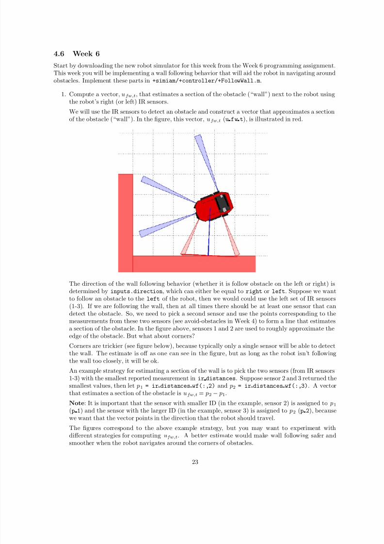
1. Compute a vector, ufw,t, that estimates a section of the obstacle (“wall”) next to the robot usingthe robot’s right (or left) IR sensors.

We will use the IR sensors to detect an obstacle and construct a vector that approximates a sectionof the obstacle (“wall”). In the figure, this vector, ufw,t (u fw t), is illustrated in red.

The direction of the wall following behavior (whether it is follow obstacle on the left or right) isdetermined by inputs.direction, which can either be equal to right or left. Suppose we wantto follow an obstacle to the left of the robot, then we would could use the left set of IR sensors(1-3). If we are following the wall, then at all times there should be at least one sensor that candetect the obstacle. So, we need to pick a second sensor and use the points corresponding to themeasurements from these two sensors (see avoid-obstacles in Week 4) to form a line that estimatesa section of the obstacle. In the figure above, sensors 1 and 2 are used to roughly approximate theedge of the obstacle. But what about corners?

Corners are trickier (see figure below), because typically only a single sensor will be able to detectthe wall. The estimate is off as one can see in the figure, but as long as the robot isn’t followingthe wall too closely, it will be ok.

An example strategy for estimating a section of the wall is to pick the two sensors (from IR sensors

1-3) with the smallest reported measurement in ir distances. Suppose sensor 2 and 3 returned thesmallest values, then let p1 = ir distances wf(:,2) and p2 = ir distances wf(:,3). A vectorthat estimates a section of the obstacle is ufw,t = p2 − p1.

Note: It is important that the sensor with smaller ID (in the example, sensor 2) is assigned to p1

(p 1) and the sensor with the larger ID (in the example, sensor 3) is assigned to p2 (p 2), becausewe want that the vector points in the direction that the robot should travel.

The figures correspond to the above example strategy, but you may want to experiment withdifferent strategies for computing ufw,t. A better estimate would make wall following safer andsmoother when the robot navigates around the corners of obstacles.

23



2. Compute a vector, ufw,p, that points from the robot to the closest point on ufw,t.

Now that we have the vector ufw,t (represented by the red line in the figures), we need to computea vector ufw,p that points from the robot to the closest point on ufw,t. This vector is visualized asblue line in the figures and can be computed using a little bit of linear algebra:

u

fw,t = ufw,t

ufw,t, u p =

xy

, ua = p1

ufw,p = (ua − u p) − ((ua − u p) · u

fw,t)u

fw,t

ufw,p corresponds to u fw p and u

fw,t corresponds to u fw tp in the code.

Note: A small technicality is that we are computing ufw,p as the the vector pointing from therobot to the closest point on ufw,t, as if ufw,t were infinitely long.

3. Combine the two vectors, such that it can be used as a heading vector for a PID controller that

will follow the wall to the right (or left) at some distance dfw .

The last step is to combine ufw,t and ufw,p such that the robot follows the obstacle all the wayaround at some distance dfw (d fw). ufw,t will ensure that the robot drives in a direction that isparallel to an edge on the obstacle, while ufw,p needs to be used to maintain a distance dfw fromthe obstacle.

One way to achieve this is,

u

fw,p = ufw,p − dfw

ufw,p

ufw,p|,

where u

fw,p (u fw pp) is now a vector points towards the obstacle when the distance to the obstacle,d > dfw, is near zero when the robot is dfw away from the obstacle, and points away from theobstacle when d < dfw.

All that is left is to linearly combine u

fw,t and u

fw,p into a single vector ufw (u fw) that can beused with the PID controller to steer the robot along the obstacle at the distance dfw .

(Hint : Think about how this worked with uao and ugtg last week).

How to test it all

To test your code, the simulator is set up to run +simiam/+controller/FollowWall.m. First test the fol-low wall behaviour by setting obj.fw direction = ‘left’ in +simiam/+controller/+quickbot/QBSupervisor

This will test the robot following the obstacle to its left (like in the figures). Then set obj.fw direction

= ‘right’, and change in settings.xml the initial theta of the robot to π :

24



<pose x="0" y="0" theta="3.1416" />

The robot is set up near the obstacle, so that it can start following it immediately. This is a validsituation, because we are assuming another behavior (like go-to-goal) has brought us near the obstacle.Here are some tips to the test the three parts:

1. Set u fw = u fw tp. The robot starts off next to an obstacle and you should see that the red lineapproximately matches up with the edge of the obstacle (like in the figures above). The robotshould be able to follow the obstacle all the way around.

Note: Depending on how the edges of the obstacle are approximated, it is possible for the robotto peel off at one of the corners. This is not the case in the example strategy provided for the firstpart.

2. If this part is implemented correctly, the blue line should point from the robot to the closest pointon the red line.

3. Set obj.d fw to some distance in [0.04, 0.3] m. The robot should follow the wall at approximatelythe distance specified by obj.d fw. If the robot does not follow the wall at the specified distance,then u

fw,p is not given enough weight (or u

fw,t is given too much weight).



1. The only new addition to the simulator is +simiam/+controller/FollowWall.m. Everything elsemay be overwrite with the exception of QBSupervisor.m.

25



4.7 Week 7

Start by downloading the new robot simulator for this week from the Week 7 programming assignment.This week you will be combining the go-to-goal, avoid-obstacles, and follow-wall controllers into a fullnavigation system for the robot. The robot will be able to navigate around a cluttered, complex environ-ment without colliding with any obstacles and reaching the goal location successfully. Implement your

solution in +simiam/+controller/+quickbot/QBSupervisor.m.

1. Implement the progress made event that will determine whether the robot is making any progresstowards the goal.

By default, the robot is set up to switch between avoid obstacles and go to goal to navigate theenvironment. However, if you launch the simulator with this default behavior, you will notice thatthe robot cannot escape the larger obstacle as it tries to reach the goal located at (x, g) = (1.1, 1.1).The robot needs a better strategy for navigation. This strategy needs to realize that the robot isnot making any forward progress and switch to follow wall to navigate out of the obstacle.

Implement the function progress made such that it returns true if

x − xg

y − yg

< dprogress − ,

where = 0.1 (epsilon) gives a little bit of slack, and dprogress (d prog) is the closest (in terms of distance) the robot has progressed towards the goal. This distance should be set using the functionset progress point before switching to the follow wall behavior in the third part.

2. Implement the sliding left and sliding right events that will serve as a criterion for whetherthe robot should continue to follow the wall (left or right) or switch back to the go-to-goal behavior.

While the lack of progress made will trigger the navigation system into a follow wall behavior,we need to check whether the robot should stay in the wall following behavior, or switch back togo to goal. We can check whether we need to be in the sliding mode (wall following) by testing if σ1 > 0 and σ2 > 0, where

ugtg uao

σ1σ2

= ufw .

Implement this test in the function sliding left and sliding right. The test will be the samefor both functions. The difference is in how ufw is computed.

3. Implement the finite state machine that will navigate the robot to the goal located at (xg, yg) =(1.1, 1.1) without colliding with any of the obstacles in the environment.

Now, we are ready to implement a finite state machine (FSM) that solves the full navigationproblem. A finite state machine is nothing but a set of if/elseif/else statements that first checkwhich state (or behavior) the robot is in, then based on whether an event (condition) is satisfied,the FSM switches to another state or stays in the same state. Some of the logic that should be partof the FSM is:

(i) If at goal, then switch to stop.

(ii) If unsafe, then switch to state avoid obstacles.

(iii) If in state go to goal and at obstacle, then check whether the robot needs to slide left orslide right. If so set progress point, and switch to state follow wall (with inputs.direction

equal to right or left depending on the results of the sliding test).

(iv) If in state follow wall, check whether progress made and the robot does not need toslide slide left (or slide right depending on inputs.direction). If so, switch to statego to goal, otherwise keep following wall.

You can check an event using obj.check event(‘name-of-event’) and switch to a different stateusing obj.switch to state(‘name-of-state’).

26



How to test it all

To test your code, the simulator is set up to run a simple FSM that is unable to exit the large obstacleand advance towards the goal.

1. Test the first part with the third part.

2. Test the second part with the third part.

3. Testing the full navigation systems is mostly a binary test: does the robot successfully reach thegoal located at (xg, yg) = (1.1, 1.1) or not? However, let us consider a few key situations that willlikely be problematic.

(i) First, the default code has the problem that the robot is stuck inside the large obstacle. Thereason for this situation is that avoid obstacle is not enough to push the robot far enough wayfrom the obstacle, such that when go-to-goal kicks back in, the robot is clear of the obstacleand has a free path towards the goal. So, you need to make sure that the robot realizes thatno progress towards the goal is being made and that wall following needs to be activated forthe robot to navigate out of the interior of the large obstacle.

(ii) Second, assuming that the robot has escaped the interior of the large obstacle and is in wallfollowing mode, there is a point at which progress is again being made towards the goal andsliding is no longer necessary. The robot should then stop wall following and resume its go-to-goal behavior. A common problem is that the robot either continues to follow the edge of thelarge obstacle and never makes the switch to go-to-goal. Another common problem is that theFSM switches to the go-to-goal behavior before the robot has the chance to escape the interiorof the large obstacle using wall following. Troubleshoot either problem by revisiting the logicthat uses the progress made and sliding left (sliding right) events to transition fromfollow wall to go to goal.

Remember that adding fprintf calls to different parts of your code can help you debug yourproblems. By default, the supervisor prints out the state that it switches to.



1. Everything may be overwrite with the exception of QBSupervisor.m.

Documents

Manual Do Simulador