Magnetic Resonance Imaging-derived Flow parameters for the

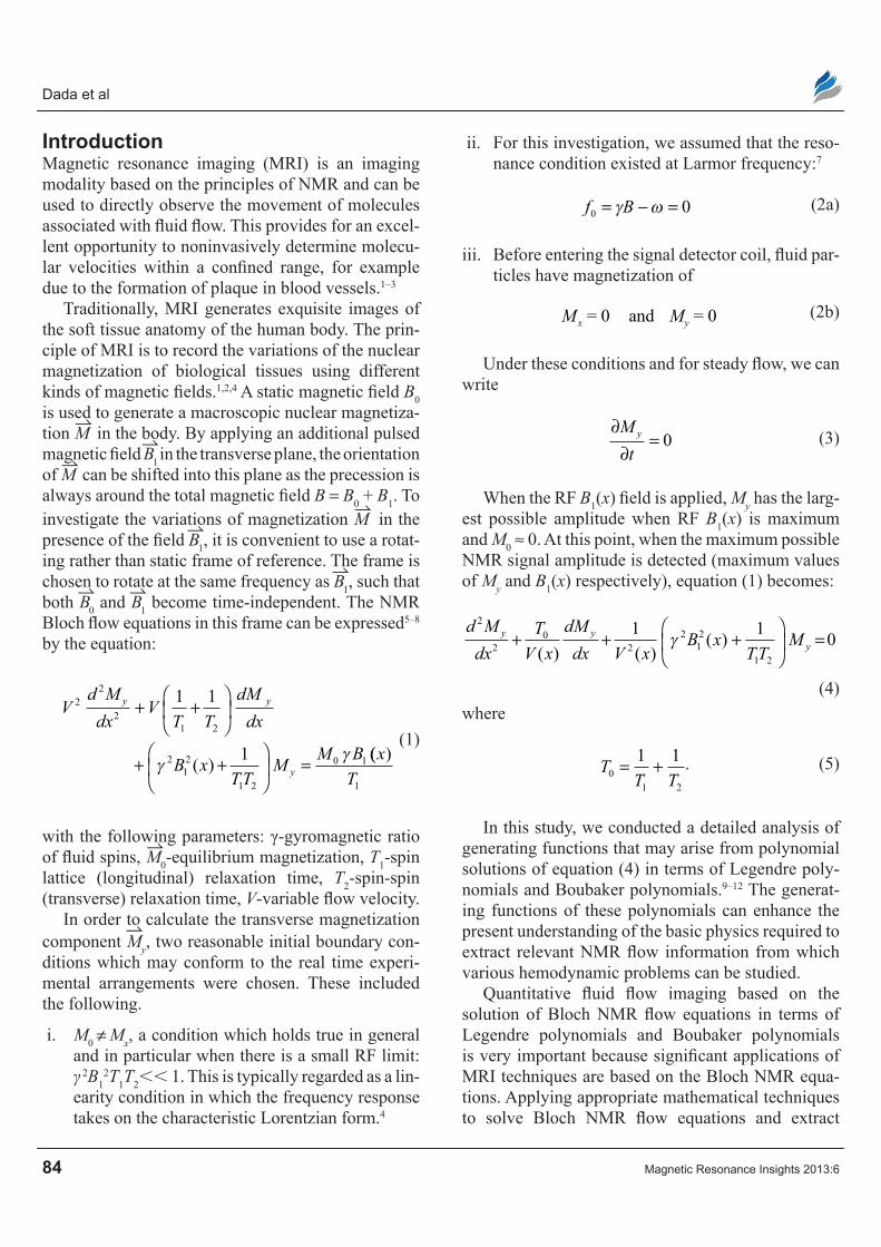
Magnetic Resonance Insights 2013:6 83–93

doi: 10.4137/MRI.S12195

This article is available from http://www.la-press.com.

© the author(s), publisher and licensee Libertas Academica Ltd.

This is an open access article published under the Creative Commons CC-BY-NC 3.0 license.

Open AccessFull open access to this and thousands of other papers at

http://www.la-press.com.O R I g I N A L R e S e A R C h

Magnetic Resonance Insights 2013:6 83

Magnetic Resonance Insights

Abstract: Nuclear magnetic resonance (NMR) allows for fast, accurate and noninvasive measurement of fluid flow in restricted and non-restricted media. The results of such measurements may be possible for a very small B0 field and can be enhanced through detailed examination of generating functions that may arise from polynomial solutions of NMR flow equations in terms of Legendre polynomials and Boubaker polynomials. The generating functions of these polynomials can present an array of interesting possibilities that may be useful for understanding the basic physics of extracting relevant NMR flow information from which various hemodynamic problems can be carefully studied. Specifically, these results may be used to develop effective drugs for cardiovascular-related diseases.

Keywords: Bloch NMR flow equations, NMR transverse magnetization, Legendre polynomials, Boubaker polynomials, rotational diffusion coefficient, cardiovascular diseases, drug discovery

Magnetic Resonance Imaging-derived Flow parameters for the Analysis of cardiovascular Diseases and Drug Development

Dada O. Michael1, Awojoyogbe O. Bamidele1, Adesola O. Adewale1 and Boubaker Karem2

1Department of Physics, Federal University of Technology, P.M.B. 65, Minna, Niger State, Nigeria. 2UPDS/eSSTT/63 Rue Sidi Jabeur, 5100 Mahdia, Tunisia. Corresponding author email: [email protected]

http://dx.doi.org/10.4137/MRI.S12195

http://www.la-press.com

http://creativecommons.org/licenses/by-nc/3.0/



http://www.la-press.com/magnetic-resonance-insights-journal-j115

mailto:[email protected]

84 Magnetic Resonance Insights 2013:6

Dada et al

IntroductionMagnetic resonance imaging (MRI) is an imaging modality based on the principles of NMR and can be used to directly observe the movement of molecules associated with fluid flow. This provides for an excel-lent opportunity to noninvasively determine molecu-lar velocities within a confined range, for example due to the formation of plaque in blood vessels.1–3

Traditionally, MRI generates exquisite images of the soft tissue anatomy of the human body. The prin-ciple of MRI is to record the variations of the nuclear magnetization of biological tissues using different kinds of magnetic fields.1,2,4 A static magnetic field B0 is used to generate a macroscopic nuclear magnetiza-tion M in the body. By applying an additional pulsed magnetic field B1 in the transverse plane, the orientation of M can be shifted into this plane as the precession is always around the total magnetic field B = B0 + B1. To investigate the variations of magnetization M in the presence of the field B1, it is convenient to use a rotat-ing rather than static frame of reference. The frame is chosen to rotate at the same frequency as B1, such that both B0 and B1 become time-independent. The NMR Bloch flow equations in this frame can be expressed5–8 by the equation:

Vd Mdx

VT T

dMdx

B xTT

M M B

y y

y

22

21 2

212

1 2

0 1

1 1

1

+ +

+ +

γ

γ( ) = (( )xT1

(1)

with the following parameters: γ-gyromagnetic ratio of fluid spins, M0-equilibrium magnetization, T1-spin lattice (longitudinal) relaxation time, T2-spin-spin (transverse) relaxation time, V-variable flow velocity.

In order to calculate the transverse magnetization component M

y, two reasonable initial boundary con-ditions which may conform to the real time experi-mental arrangements were chosen. These included the following.

i. M0 ≠ Mx, a condition which holds true in general and in particular when there is a small RF limit: γ 2B1

2T1T2 1. This is typically regarded as a lin-earity condition in which the frequency response takes on the characteristic Lorentzian form.4

ii. For this investigation, we assumed that the reso-nance condition existed at Larmor frequency:7

f B0 0= − =γ ω (2a)

iii. Before entering the signal detector coil, fluid par-ticles have magnetization of

M Mx y= 0 and = 0 (2b)

Under these conditions and for steady flow, we can write

∂

∂=

Mt

y 0 (3)

When the RF B1(x) field is applied, My has the larg-est possible amplitude when RF B1(x) is maximum and M0 ≈ 0. At this point, when the maximum possible NMR signal amplitude is detected (maximum values of My and B1(x) respectively), equation (1) becomes:

d Mdx

TV x

dMdx V x

B xTT

My yy

2

20

22

12

1 2

1 1 0+ + +

=

( ) ( )( )γ

(4)where

TT T0

1 2

1 1= + . (5)

In this study, we conducted a detailed analysis of generating functions that may arise from polynomial solutions of equation (4) in terms of Legendre poly-nomials and Boubaker polynomials.9–12 The generat-ing functions of these polynomials can enhance the present understanding of the basic physics required to extract relevant NMR flow information from which various hemodynamic problems can be studied.

Quantitative fluid flow imaging based on the solution of Bloch NMR flow equations in terms of Legendre polynomials and Boubaker polynomials is very important because significant applications of MRI techniques are based on the Bloch NMR equa-tions. Applying appropriate mathematical techniques to solve Bloch NMR flow equations and extract


MRI-derived flow analysis for cardiovascular diseases and drug development


relevant NMR flow parameters to accurately monitor the fluid state is very important for MRI studies.

Mathematical ModelEquation (4) was obtained under conditions of when the RF B1(x) field is applied and My has a maximum value, M0 = 0. Equation (4) can be written in the form:

d Mdx

TV x

dMdx

TV x

My y gy

2

20

2 0+ + =( ) ( )

(6)

The fluid velocity V is dependent on the spatial variable x. We may therefore write that:

T

V x lCot x

l0 1

( )= (7)

where l = l (x) is a parameter in the unit of length and Cot x

l is a cotangent function of x

l. Equation (6) is

based on the condition that:

γ 212

1 2

1B xTT

( ) (8)

where

TT Tg = 1

21

. (9)

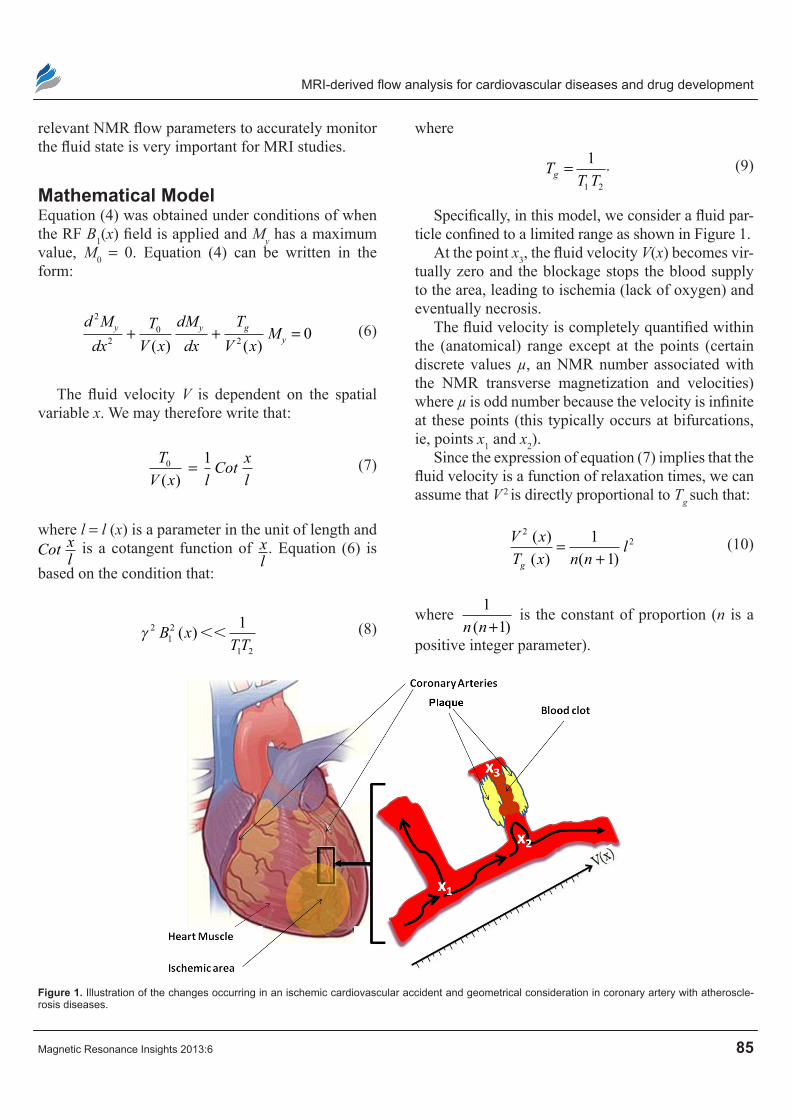
Specifically, in this model, we consider a fluid par-ticle confined to a limited range as shown in Figure 1.

At the point x3, the fluid velocity V(x) becomes vir-tually zero and the blockage stops the blood supply to the area, leading to ischemia (lack of oxygen) and eventually necrosis.

The fluid velocity is completely quantified within the (anatomical) range except at the points (certain discrete values µ, an NMR number associated with the NMR transverse magnetization and velocities) where µ is odd number because the velocity is infinite at these points (this typically occurs at bifurcations, ie, points x1 and x2).

Since the expression of equation (7) implies that the fluid velocity is a function of relaxation times, we can assume that V 2 is directly proportional to Tg such that:

V xT x n n

lg

221

1( )( ) ( )

=+

(10)

where 11n n( )+

is the constant of proportion (n is a

positive integer parameter).

Figure 1. Illustration of the changes occurring in an ischemic cardiovascular accident and geometrical consideration in coronary artery with atheroscle-rosis diseases.



Dada et al

From equations (10), we can write:

d Mdx l

Cot xl

dMdx l

n n My yy

2

2 2

1 1 1 0+ + + =( ) (11)

Sin xl

d Mdx l

Cos xl

dMdx l

Sin xl

n n My yy

2

2 2

1 1 1 0+ + + =( )

(12)

ddx

Sin xl

dMdx l

Sin xl

n n Myy

+ + =1 1 02 ( ) (13)

If we define ε = Cos xl

, equation (13) becomes

dd

dMd l

Sin xl l

Sin xl

n n Myyε

εε

( ) ( )1 1 1 1 022 2−

+ + =

(14)

Dividing equation (14) through by 12l

Sin xl , we

obtain a Legendre differential equation:

1 2 1 02

2

2−( ) − + + =εε

εε

d Md

dMd

n n My yy( ) (15)

The solution of equation (15) is of the form:13–16

M M C P C Qy yn n n( ) ( ) ( ) ( )ε ε ε ε= = += …1 2 n 0,1,2,3,

(16)

where Pn (ε) and Qn

(ε) are the Legendre polynomials of the first type and second type, respectively, and C1 and C2 are constants. It is worthy of note that Pn

(ε) and Qn

(ε) are two linearly independent solutions to equation.15 Hence, C2 must be equal to zero and C1 is equal to unity:

M P n pp n p n pyn n

p

nn p

p( ) ( ) ( ) ( )!

! ( ) ! ( )!ε ε ε= = − −

− −−

=∑ 1 2 2

2 22

0

Θ

(17)

where

Θ =+ − −( )2 1 1

4n n( )

(18)

Equation (17) can be factorized by its own first term. Setting m = n – p:

M nn n

n pp

n pn p

yn n

p

p

nn

( ) ( )!! !

( ) ( )!

( )!( )!

ε

ε

=

− − − −−=

∑

22

1 4 120

×ξ ( )

−−

=

2

22

p

n nnn n

B xl

( )!! !

cos (19)

where Bn (ε) denote the Boubaker polynomials.6–9

BBBB

BB

0

1

22

33

44

55 3

1

2

2

3

( )( )

( )

( )

( )

( )

εε ε

ε ε

ε ε ε

ε ε

ε ε ε ε

==

= +

= +

= −

= − −

or

B

B xl

B xl

B xl

xl

B

0 =

=

=

+

=

+

1

2

1

2

2

3

3

4

cos

cos

cos cos

==

−

=

−

−

cos

cos cos cos

xl

B xl

xl

xl

4

5

5 3

2

3

(20)

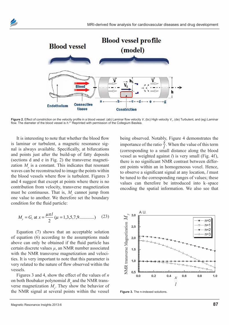
Bn (ε) is a polynomial in ε. The elementary first n-

indexed solutions are represented in Figure 3.

DiscussionIn Figure 3, the curves correspond to the vanishing modes of the expression obtained for the transverse magnetization in Equations (17) and (19). This fea-ture agrees with the results obtained by Kobayashi et al,16 Chapman et al,17 and Donnat et al.18

The case n = 0 (Fig. 3) initially corresponds to the reduced equation:

1 2 022

2−( ) − =εε

εε

d Md

dMd

y y (21)

which has the solution:

M G Gy ( ) lnε

εε

= − +−1

2

211

(G1 and G2 are constants)

(22)




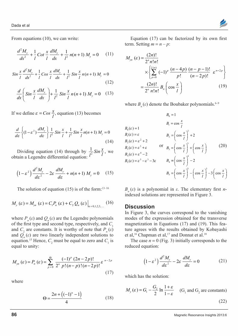
Figure 2. Effect of constriction on the velocity profile in a blood vessel: (ab) Laminar flow velocity V, (bc) high velocity V1, (de) Turbulent, and (eg) Laminar flow. The diameter of the blood vessel is h.21 Reprinted with permission of the Collegium Basilea.

It is interesting to note that whether the blood flow is laminar or turbulent, a magnetic resonance sig-nal is always available. Specifically, at bifurcations and points just after the build-up of fatty deposits (sections d and e in Fig. 2) the transverse magneti-zation My is a constant. This indicates that resonant waves can be reconstructed to image the points within the blood vessels where flow is turbulent. Figures 3 and 4 suggest that except at points where there is no contribution from velocity, transverse magnetization must be continuous. That is, My cannot jump from one value to another. We therefore set the boundary condition for the fluid particle:

M G x ly = = =1 2

at µπµ( 1,3,5,7,9.............) (23)

Equation (7) shows that an acceptable solution of equation (6) according to the assumptions made above can only be obtained if the fluid particle has certain discrete values µ, an NMR number associated with the NMR transverse magnetization and veloci-ties. It is very important to note that this parameter is very related to the nature of flow observed within the vessels.

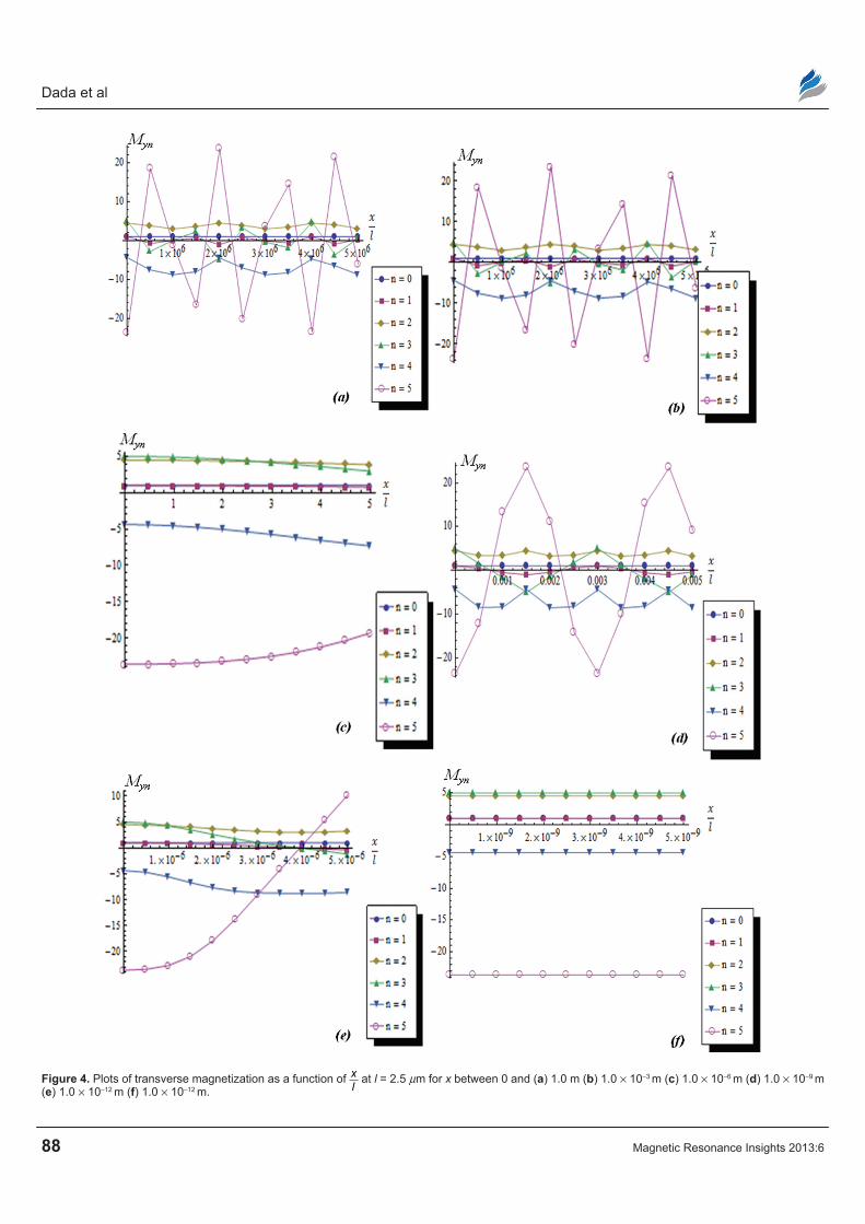
Figures 3 and 4, show the effect of the values of n on both Boubaker polynomial Bn and the NMR trans-verse magnetization My. They show the behavior of the NMR signal at several points within the vessel

being observed. Notably, Figure 4 demonstrates the importance of the ratio xl . When the value of this term (corresponding to a small distance along the blood vessel as weighted against l) is very small (Fig. 4f ), there is no significant NMR contrast between differ-ent points within an in homogeneous voxel. Hence, to observe a significant signal at any location, l must be tuned to the corresponding ranges of values; these values can therefore be introduced into k–space encoding the spatial information. We also see that

Figure 3. The n-indexed solutions.



Dada et al

Figure 4. Plots of transverse magnetization as a function of xl

at l = 2.5 µm for x between 0 and (a) 1.0 m (b) 1.0 × 10−3 m (c) 1.0 × 10−6 m (d) 1.0 × 10−9 m (e) 1.0 × 10−12 m (f) 1.0 × 10−12 m.




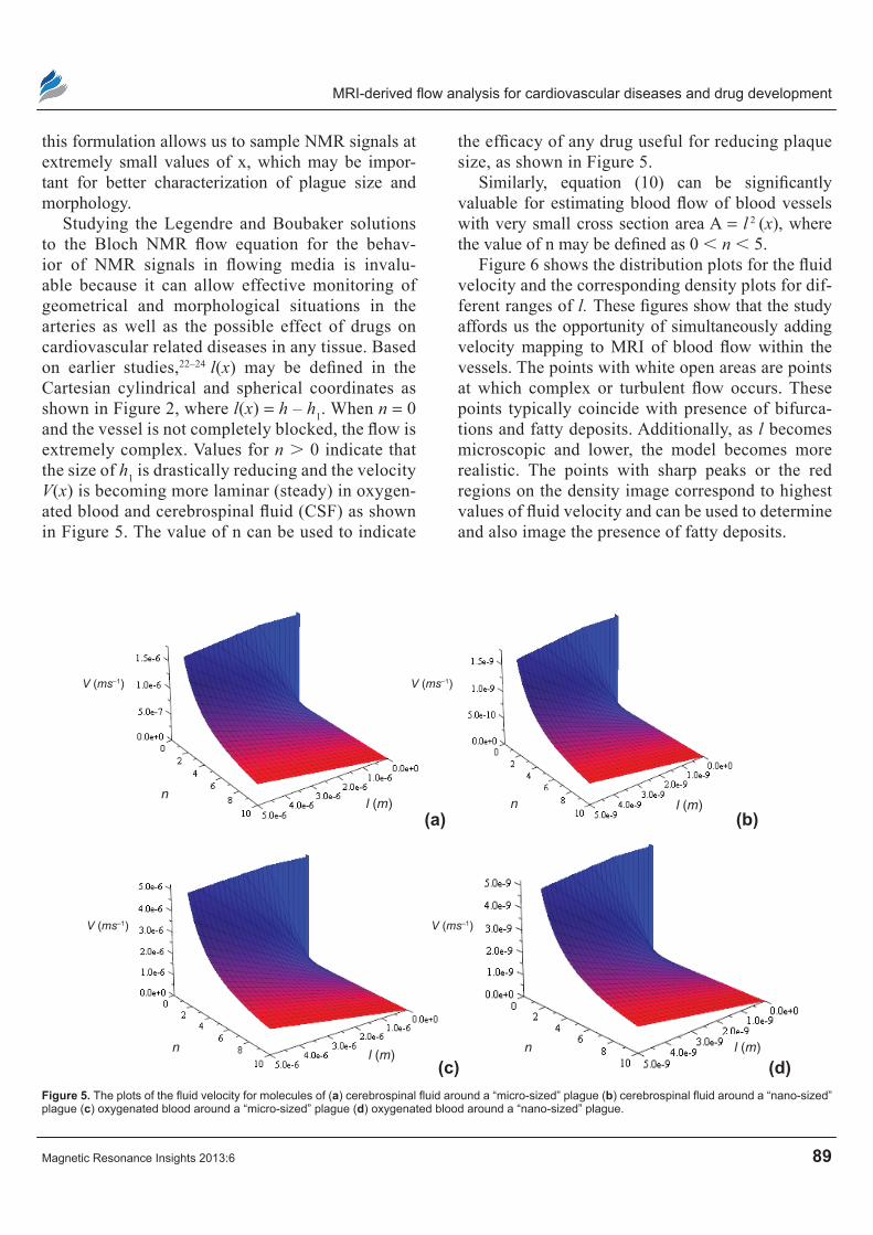
this formulation allows us to sample NMR signals at extremely small values of x, which may be impor-tant for better characterization of plague size and morphology.

Studying the Legendre and Boubaker solutions to the Bloch NMR flow equation for the behav-ior of NMR signals in flowing media is invalu-able because it can allow effective monitoring of geometrical and morphological situations in the arteries as well as the possible effect of drugs on cardiovascular related diseases in any tissue. Based on earlier studies,22–24 l(x) may be defined in the Cartesian cylindrical and spherical coordinates as shown in Figure 2, where l(x) = h – h1. When n = 0 and the vessel is not completely blocked, the flow is extremely complex. Values for n 0 indicate that the size of h1 is drastically reducing and the velocity V(x) is becoming more laminar (steady) in oxygen-ated blood and cerebrospinal fluid (CSF) as shown in Figure 5. The value of n can be used to indicate

the efficacy of any drug useful for reducing plaque size, as shown in Figure 5.

Similarly, equation (10) can be significantly valuable for estimating blood flow of blood vessels with very small cross section area A = l 2 (x), where the value of n may be defined as 0 n 5.

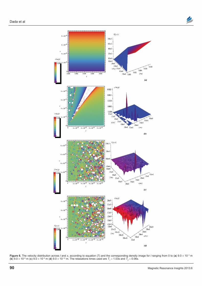
Figure 6 shows the distribution plots for the fluid velocity and the corresponding density plots for dif-ferent ranges of l. These figures show that the study affords us the opportunity of simultaneously adding velocity mapping to MRI of blood flow within the vessels. The points with white open areas are points at which complex or turbulent flow occurs. These points typically coincide with presence of bifurca-tions and fatty deposits. Additionally, as l becomes microscopic and lower, the model becomes more realistic. The points with sharp peaks or the red regions on the density image correspond to highest values of fluid velocity and can be used to determine and also image the presence of fatty deposits.

(b)(a)l (m)

nl (m)

V (ms–1) V (ms–1)

n

l (m) n

V (ms–1) V (ms–1)

n l (m) (c) (d)

Figure 5. The plots of the fluid velocity for molecules of (a) cerebrospinal fluid around a “micro-sized” plague (b) cerebrospinal fluid around a “nano-sized” plague (c) oxygenated blood around a “micro-sized” plague (d) oxygenated blood around a “nano-sized” plague.



Dada et al

Figure 6. The velocity distribution across l and x, according to equation (7) and the corresponding density image for l ranging from 0 to (a) 9.0 × 10−3 m (b) 9.0 × 10−6 m (c) 9.0 × 10−9 m (d) 9.0 × 10−12 m. The relaxations times used are T1 = 1.03s and T2 = 0.06s.




It may be significant to note that the rotational dif-fusion coefficient Drot can be defined from equation (7) as,19,20 considering that l is a fixed length:

D V xl Trot

g

=2

2

( )τ

(24)

Given that the translational diffusion coefficient is:

D V xTtrans

g

=2 ( )τ

, where τ is the correlation time defined

as:19,20

τ =+11n n Drot( )

(25)

For the value n = 1, My (ε) = P1(ε) = B1(ε) and the correlation time becomes

τ = 12Drot

(26)

The physical implication for when n = 0 can be interpreted as the constant magnetization where the correlation time is observed to be infinitely small.

Finally, the rotational diffusion coefficient as given in equation (23) may be written as:19,20

V xl T

k Tfg

B

r

2

2

( )τ

=

where kB is the Boltzman n constant, T is the absolute temperature of the tumbling blood molecules, and fr is the rotational friction coefficient. Therefore, the fric-tion coefficient, which provides significant informa-tion regarding molecular interactions, is given as:

f k TT n nk TT

Txlr B g

B g= + =ττ

[ ( )] cot102

2 (27)

conclusionsWe have derived the MRI signal in terms of Legendre and Boubaker polynomials. By solving the Bloch NMR flow equations under some assumptions, we obtained elementary spatial profiles of the transverse

magnetization response. The primary advantage of this approach is the potential to exploit spatial-evolution of magnetic response in the presence of a preset rotat-ing field for monitoring the effect of a drug on cardio-vascular-related diseases and to estimate blood flow rate in very small blood vessels.

Interestingly, quantification of the velocity is not a direct prediction of equation (7), but it is a conse-quence of the conditions imposed on the transverse magnetization.

In physical situations in which a fluid par-ticle is confined in space, for example, at x = βl,

where − < < +

πβ

π2 2

, most solutions behave in

an inappropriate way at the edges of the region of interest. Only for certain precisely determined veloci-ties are satisfactory solutions obtained. The bound-ary conditions which the transverse magnetization My must satisfy cannot be derived. They can be justified in part by the physical interpretation of My based on the properties of Boubaker polynomials in equation (19):

(i) My must be a well-defined functions of position,(ii) My cannot be infinite any where except at the

point x l= µπ2

(µ = even integer),(iii) My must be continuous, and not jump abruptly

from one value to another.(iv) When n = 0, and x l= µπ

2 (µ = odd integer), the

transverse magnetization is a constant and the velocity is indeterminate.

(v) The NMR transverse magnetization is directly proportional to Boubaker polynomials.

(vi) My has the same value as the Boubaker polyno-mials when n = 1.

Detailed study of these NMR flow parameters and properties of the transverse magnetization as described in this study can allow for careful optimization and 3D computer graphics of fluid flow magnetic reso-nance imaging. A simple illustration of this is given in Figure 6. The mathematical analysis presented in this study is based on the assumption made in equation (7). This was done with the goal of exploring the spa-tial evolution of the MRI signal in the presence of a preset rotating field.



Dada et al

The biological, physical, biomedical, and geo-physical applications of equations (17), (19), (23), (25), and (27) when n 1 can be used for all NMR/MRI procedures and further application of this study will be presented in separate studies. For an example of the physical properties of a drug designed to reduce the size of h1 of the fatty deposit in Figure 2 may be revealed by equations (24–27).

Notably, the parameter l in equation (7) is a length used to scale x. This parameter may be used for slice selection in spatial encoding in a typical MRI experi-ment so that l can be defined such that:

lG

= 1γ τ

(28)

where G is the applied gradient and τ is the duration of the applied gradient.4 The area A l x= 2 ( ) (which was discussed above) represents the field of view (FOV) for the voxel selected.

Author contributionsDOM, AOB, AOA and BK participated equally in the work giving rise to this manuscript. All authors reviewed and approved of the final manuscript.

AcknowledgementThe authors acknowledge the support of Federal Uni-versity of Technology Minna through the STEP—B research scheme. The meticulous review of this arti-cle is highly appreciated.

competing InterestsAuthors disclose no potential conflicts of interest.

Disclosures and ethicsAs a requirement of publication the authors have pro-vided signed confirmation of their compliance with ethical and legal obligations including but not lim-ited to compliance with ICMJE authorship and com-peting interests guidelines, that the article is neither under consideration for publication nor published elsewhere, of their compliance with legal and ethi-cal guidelines concerning human and animal research participants (if applicable), and that permission has

been obtained for reproduction of any copyrighted material. This article was subject to blind, indepen-dent, expert peer review. The reviewers reported no competing interests.

References 1. Ngo JT, Morris PG. General solution to the NMR excitation problem for

non-interacting spins. Magn Reson Med. 1987;5(3):217–237. 2. Rourke DE, Morris PG. The inverse scattering transform and its use in the

exact inversion of the Bloch equation for non-interacting spins. Journal of Magnetic Resonance. 1992;99(1):118–138.

3. Rourke DE, Morris PG. Half solitons as solutions to the Zakharov-Shabat eigenvalue problem for rational reflection coefficient with application in the design of selective pulses in nuclear magnetic resonance. Phys Rev A. 1992;46(7):3631–3636.

4. Cowan BP. (1997). Nuclear Magnetic Resonance and Relaxation, 1sted. Cambridge: Cambridge University Press.

5. Awojoyogbe OB, Dada OM, Faromika OP, Dada OE. Mathematical concept of the Bloch flow equations for general magnetic resonance imaging: are view. Concepts in Magnetic Resonance Part A. 2011;38A(3):85–101.

6. Dada OM, Faromika OP, Awojoyogbe OB, Dada OE, Aweda MA. The impact of geometry factors on NMR diffusion measurements by the Stejskal and Tanner pulsed gradients method. International Journal of Theoretical Physics, Group Theory and Nonlinear Optics. 2011;15(1–2).

7. Awojoyogbe OB. Analytical solution of the time-dependent Bloch NMR equations: atranslational mechanical approach. Physica A. 2004;339(3–4): 437–460.

8. Awojoyogbe OB, Boubaker K. A solution to Bloch NMR flow equations for the analysis of homodynamic functions of blood flow system using m-Bou-baker polynomials. Current Applied Physics. 2009;9(1):278–283.

9. Boubaker K. On modified Boubaker polynomials: some differential and analytical properties of the new polynomials issued from an attempt for solving bi-varied heat equation. Trends in Applied Science Research. 2007;2(6):540–544.

10. Labiadh H, Boubaker K. A Sturm-Liouville shaped characteristic dif-ferential equation as a guide to establish a quasi-polynomial expression to the Boubaker polynomials. Journal of Differential Equations and CP. 2007;2:117–133.

11. Labiadh H, Dada M, Awojoyogbe OB, Ben Mahmoud KB, Bannour A. Establishment of an ordinary generating function and a Christoffel- Darboux type first-order differential equation for the heat equation related Boubaker-Turki polynomials, Journal of Differential Equations and CP. 2008;1:51–66.

12. Antonov VA, Timoshkova EI, Kholoshevnikov KV. An Introduction to The-ory of Newton’s Potential [in Russian]. Moscow: Nauka, 1988.

13. Suetin PK. Classical Orthogonal Polynomials [in Russian]. 2nd ed. Moscow: Nauka, 1979.

14. Gradshteyn IS, Ryzhik IM. Tables of Integrals, Series, and Products [in Russian]. 2nd ed. Waltham, MA: Academic Press, 1994.

15. Bateman H, Erd´elyi A. Higher Transcendental Functions, vol. 3: Ellip-tic and Modular Functions. Lame and Mathieu Functions, New York, NY: McGraw–Hill, 1955; Russian transl: Moscow, 1967.

16. Kobayashi A, Okayama Y, Yamazaki N. 31P-NMR magnetization transfer study of reperfused rat heart. Mol Cell Biochem. 1993;119(1–2):121–127.

17. Chapman BE, Kuchel PW. Fluoride trans membrane exchange in human erythrocytes measured with 19F NMR magnetization transfer. Eur Biophys J. 1990;19(1):41–45.

18. Donnat P, Rauch J. Global solvability of the Maxwell-Bloch equations from nonlinear optics. Archive for Rational Mechanics and Analysis. 1996; 136:291–303.

19. Loman A, Gregor I, Stutz C, Mund M, Enderlein J. Measuring rotational diffusion of macromolecules by fluorescence correlation spectroscopy. Pho-tochem Photobiol Sci. 2010;9(5):627–636.




20. Martínez MC, García de la Torre J. Brownian dynamics simulation of restricted rotational diffusion. Biophys J. 1987;52(2):303–310.

21. Dada M, Awojoyogbe OB, Moses FO, Ojambati OS, De DK, Boubaker K. A mathematical analysis of stenosis geometry, NMR magnetizations and signals based on the Bloch NMR flow equations, Bessel and Boubaker polynomial expansions. Journal of Biological Physics and Chemistry. 2009;9(3):101–106.

22. Awojoyogbe OB. A mathematical model of Bloch NMRequations for quantitative analysis of blood flow in blood vessels with changing cross-section II. Physica A. 2003;323(C):534–550.

23. Awojoyogbe OB. A mathematical model of Bloch NMR equations for quan-titative analysis of blood flow in blood vessels with changing cross-section I. Physica A. 2002;303:163–175.


Documents

Magnetic Resonance Imaging-derived Flow parameters for the