Embed Size (px)
Citation preview
ESTIMATORS FOR GENETIC PARAMETERS OF POPULATIONS DERIVED
FROM PARENTS OF A DIALLEL MATING
R. O. Kuehl and J. O. Rawlings
Institute of StatisticsMimeo Series No. 384
-'-"
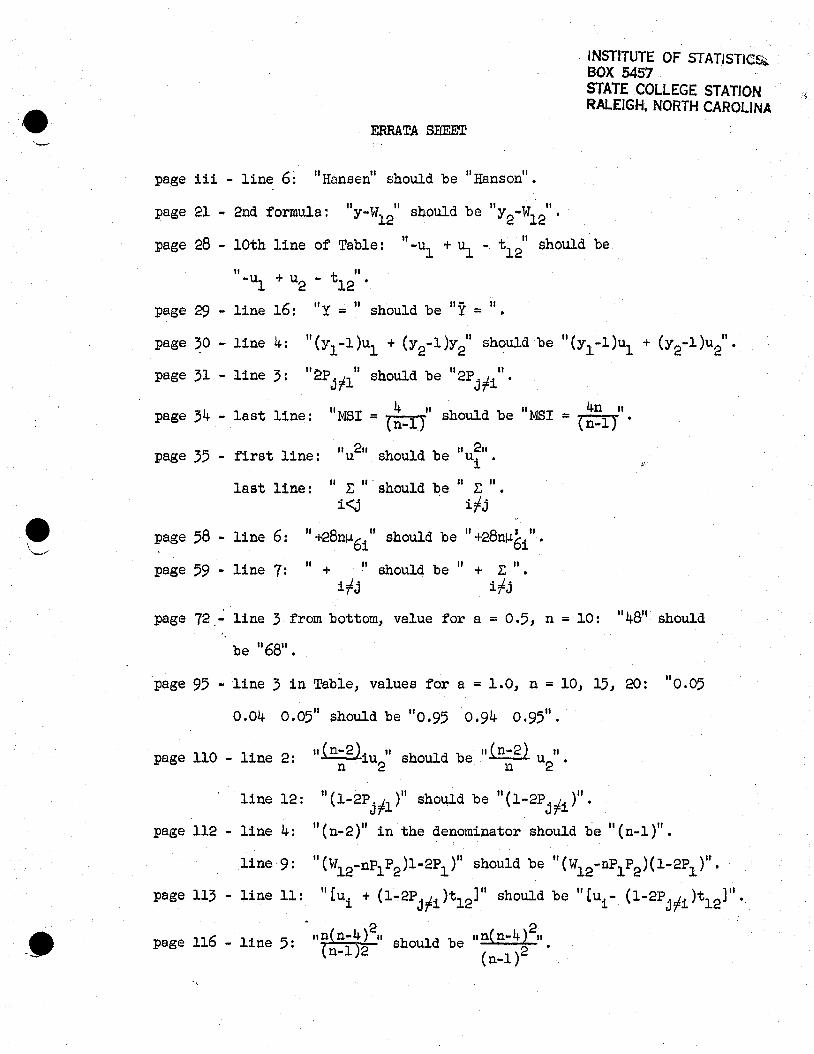
INSTITUTE OF STATISTICSi.BOX 5457STATE COLLEGE STATIONRALEIGH. NORTH CAROLINA
ERRATA SnEEr
page iii - line 6: "Hansenll should be "Hansonll.
page 21 - 2nd formula: IIY- W1211 should be IY2-W12"'
8 II II h uld bpage 2 - lOth line of Table: -ul + ul - t l2 S 0 e
II -ul + u2 - t1211.
page 29 - line 16: "y = " should be 111' = "•
page 30 - line 4: II(Yl -l)Ul
+ (y2-l)y
211 should be lI(yl -l)ul
31 II~" . II IIpage - line 3: C.Pjfl should be 2Pjfi
.
page 34 - last line: II MSI = (~-1)' should be "MSI = (~~li"
"u211 II 2"page 35 - first line: should be ui •
last line: II 1: II· should be II 1: " •i<j irj
58 1 6 "8 "hId 118'"page - ine : +2 nJ..L6i s ou be +2 nl-161 •
page 59 - line 7: II + "should be II + .E II •irj irj
.'
page 72,- line 3 from bottom, value for a = 0.5, n = 10: 114811. should
"
be 1168" •
page 95 - line 3 in Table, values for a = 1.0, n = 10, 15, 20: "0.05
0.04 0.05" should be "0.95 0.94 0.95",
page 110 - line 2:
line 12:
page 112 - line 4:
,,(n-2)i" h ldb lI[n-,gl IIn u2 s ou e. n u2 •
II()II " ( )"l-2Pjrl should be l-2Pj# 'II ( )11 . . ".( )11n-2 in the deno~nator should be n-l..
••li 9 "(w P )1 1"\ )11 h ld b "(W )(1""')"ne: 12-nPl 2 -c.P1 s ou e 12-nPI P2 -c.P1 •
page 113 - line 11: II[Ui + (1-2Pjri)t12]" should be "[ui - (1-2Pjri)t12]"'
• 2 2page 116 - 1· 5' "r(n-j) II b uld b "n(n-4) IIJ.ne, n-l 2 so e 2'
(n-l)
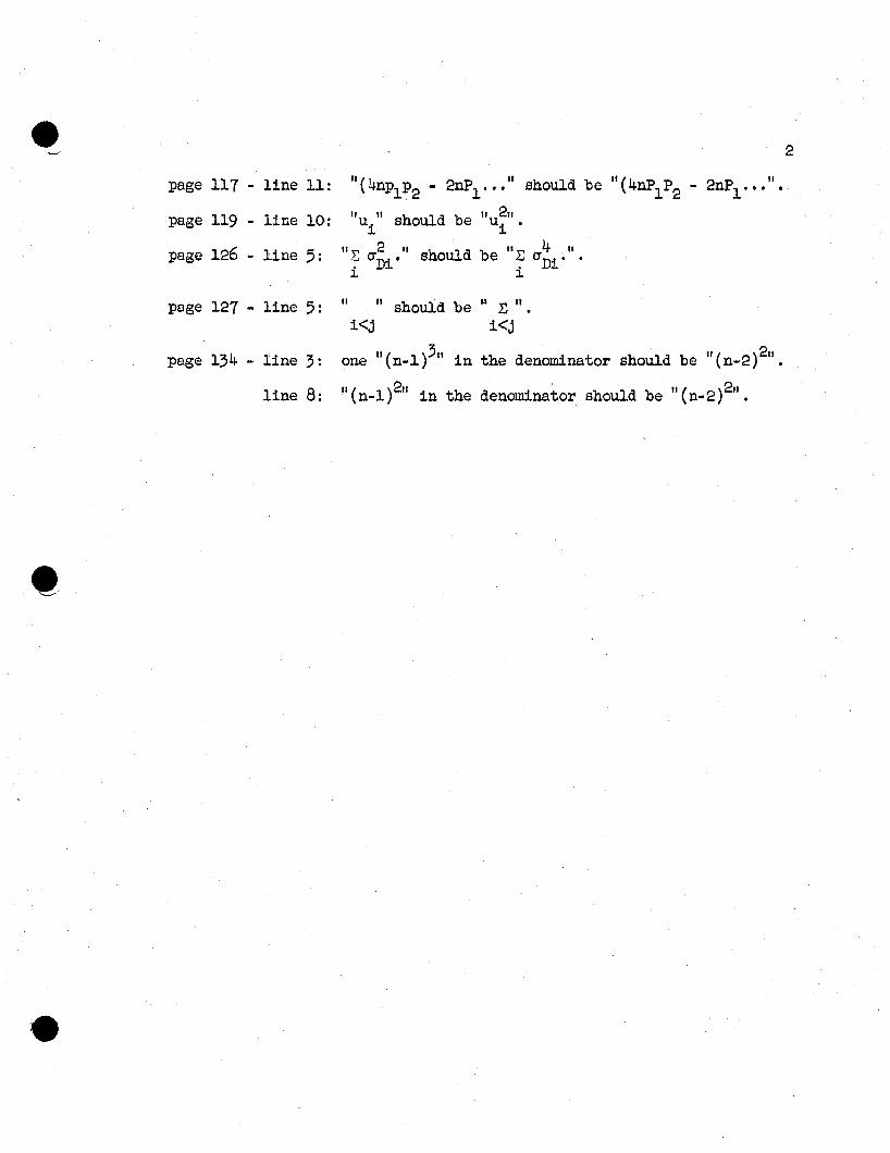
page 117 - line 11:
page 119 - line 10:
page 126 - line 5:
11(, 2P II huldb~nP1P2 - n 1'" s 0 e
" II h uld b "2,,ui s 0 e ui '
" >' 2 " should be "" 4 "":' crDi' :-- crDi , ,~ ~
2
page 127 - line 5: IIII should be " .E 11 ,
page 134 - line 3:
line 8:
i<j i<j
one "(n_I)311 in the denominator should be II (n_2)211,
II ( )211 . " II ( )211. n-1 in the denomJ.nator should be n-2 ,
iv
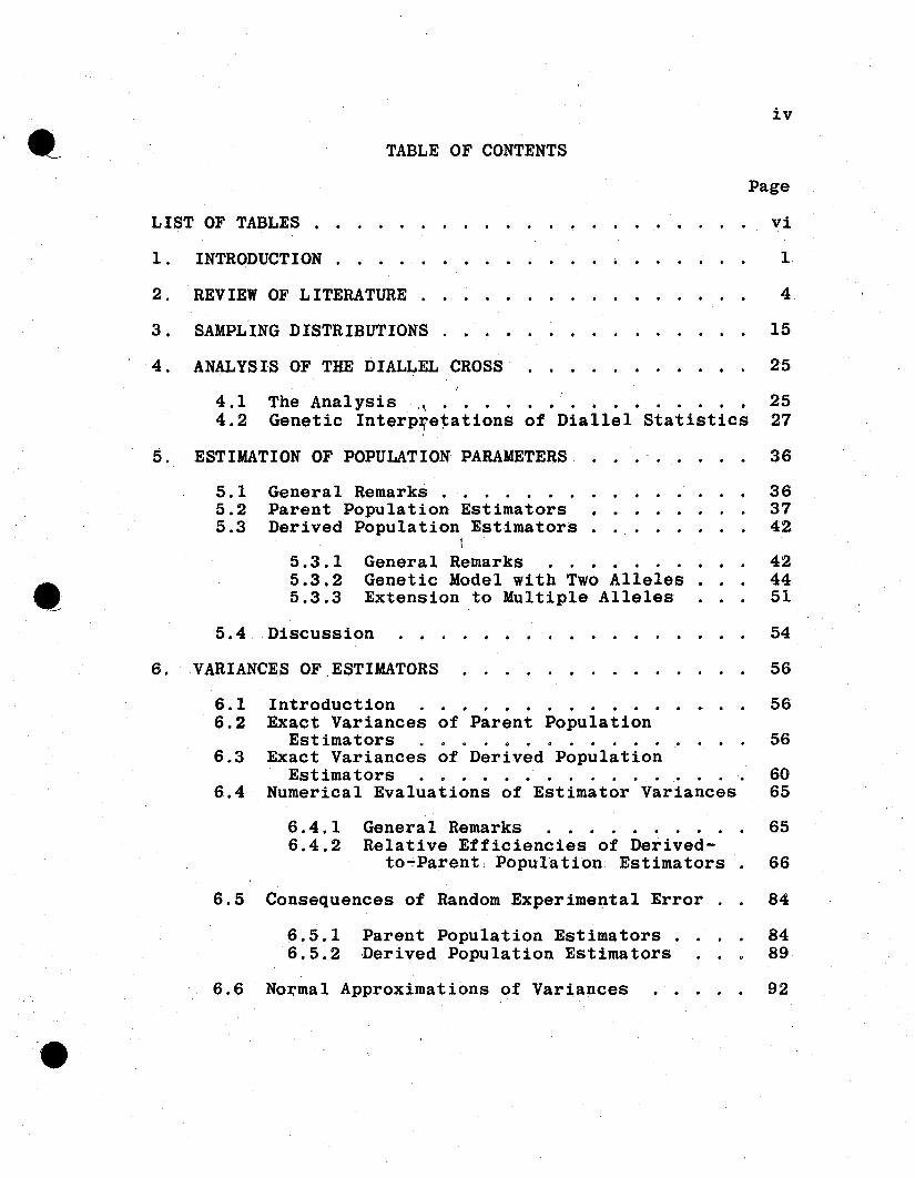
TABLE OF CONTENTS
Page
LIST OF TABLES • .
1. INTRODUCTION.
vi
1
3. SAMPLING DISTRIBUTIONS
4. ANALYSIS OF THE DIAL~EL CROSS
2. REVIEW OF LITERATURE 4
15
25
4.1 The Analysis .~ . . . . . . . .. .... 254.2 Genetic InterP7e~ations of Dial1e1 Statistics 27
5.3.15.3.25.3.3
36
363742
424451
General Remarks . '. . . . . . . . . .Parent Population Estimators • . . . . .Derived Population Estimators . . . . . .
I
General Remarks . . . . . . . .Genetic Model With Two Alleles .Extension to Multiple Alleles .
5. ESTIMATION OF POPULATION PARAMETERS
5.15.25.3
5.4 Discussion 54
56
56
56
6065
Introduction . . . . . . . . . . .Exact Variances of Parent Population
Estimators 0 • 0 • 0 • 0 • • • • • 0 • • •
Exact Variances of Derived PopulationEstimators . . . . . . . . . .
Numerical Evaluations of Estimator Variances
6.3
6.4
6. VARIANCES OF.ESTIMATORS
6.16.2
6.4.1 General Remarks . . . . . . . . . . 656.4.2 Relative Efficiencies of Derived-
to "i'Parent , Popula tion. Estimators. 66
6.5 Consequences of Random Experimental Error. . 84
6.5.1 Parent Population Estimators. . 846.5.2 ·Derived Population Estimators . . . 89
6.6 No~mal Approximations of Variances 92
'e
v
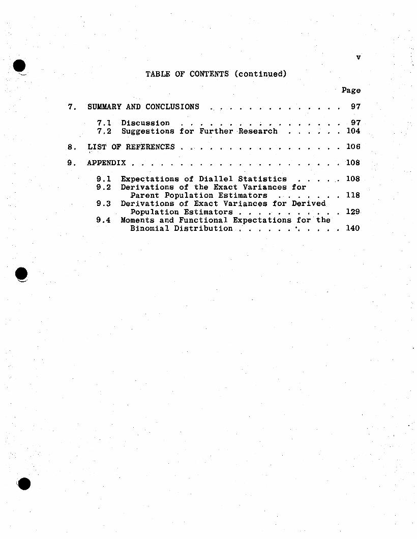
TABLE OF CONTENTS (continued)
7. SUMMARY AND CONCLUSIONS . .Page
97
7.1 Discussion . . . . . . . . • . . . . . . . . 977.2 Suggestions for Further ·Research .... 104
108
. 129
. 140
. . . 106
108
Expectations of Diallel StatisticsDerivations of the Exact Variances for
Parent Population Estimators . . . . . . . 118Derivations of Exact Variances for Derived
Population Estimators . . . . .. . .Moments and Functional Expectations for the
Binomial Distribution . . . ...•..
9.3
9.4
LIST OF REFERENCES .,
APPENDIX . . . . . .
9.19.2
8.
9.
32
>.~~&~.... l ,
vi
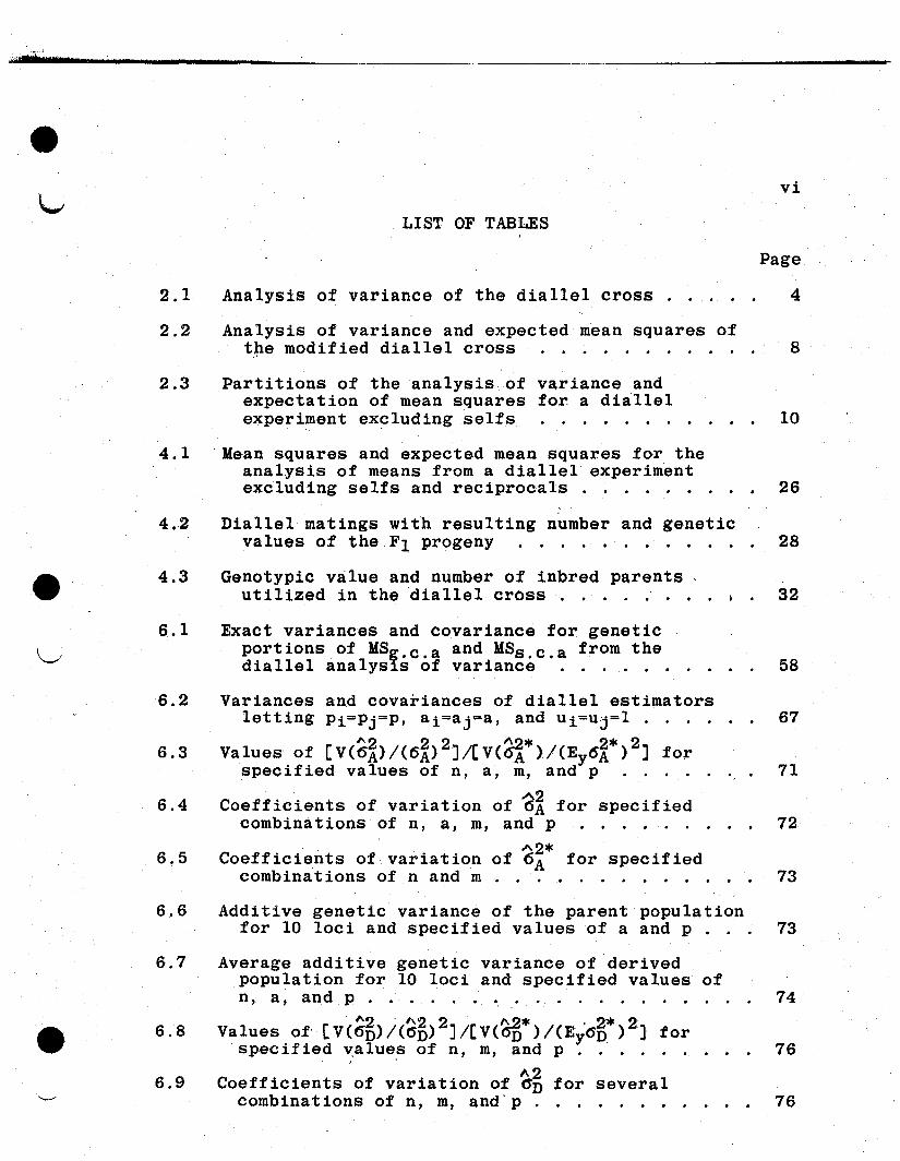
LIST OF TABLES
Page
2.1 Analysis of variance of the diallel cross. . . .. 4
2.2 Analysis of variance and expected mean squares oftp,e modified diallelcross . . . . . . . . ... 8
2.3 Partitions of the analysis of variance andexpectation of mean squares for. a diallelexperiment excluding selfs . . . . . . . 10
4.1 'Mean squares and expected mean squares for theanalysis of means from a dial leI experimentexcluding selfs and reciprocals .. ..... 26
4.2 Diallel matings with resulting number and geneticvalues of the Fl progeny . . . . . . . . . . . . 28
Genotypic value and number of inbred parents,utilized in the 'diallel cross . . ...' .
Exact variances and covariance for geneticportions of MSg . c . a and MSs . c . a from thediallel analys1s of variance . . . . . . 58
Variances and covariances of diallel estimatorsletting Pi=Pj=P, ai=aj~a, and Ui=Uj=l . ... 67
A2 2 2 ~* 2* 2Values' of [V(6A)/(6A) ]/[V(6A )j(Ey6A ) J fo~specified values of n, a, m, and p . . .,. 71
Coefficients of variation of ~X for specifiedcombinations of n, a, m, and p . . . . . . . . . 72
Coefficients of,variation of 6~* for specifiedcombinations of nand m . . .. . . . . . . . 73
Additive genetic variance of the parent populationfor 10 loci and specified valuesofa and p . . . 73
Average additive genetic variance of derivedpopulation for 10 loci and specified values ofn·, a, an.d p . . . 0 • • •• ,. • • • ., • • 74
~2 "2 2 "_2* , 2* 26.8 Values of' [V(C>j»/(O"D) J/[V«(5fi )/(EYO"D ) J for
specified v.:a1ue,s of n, m, and p . . . .. . . . . 76
6.9 Coefficients of variation of ~fi for severalcombinations of n, m, and'p . . 76
1. INTRODUCTION
The dia11e1 cross has been utilized for a riumber of
years to investigate the nature of gene action in plant
populations. Numerous analyses and interpretations of the
diallel experiment have evolved as a result of the research.
Basically, the dialle1 cross i~ its current context is con
stituted by all possible crosses among ,a set of parents.
A discussion of the modifications of the dia1le1 cross
and the associated analyses is presented in Section 2. At
least two inference populations are used in the interpreta
tion of the analysis of the dial1e1 cross. One is the ran
dom mating parent population from which the crosses are a
random sample. The second is the set of parents utilized
for the dial1el cross. Much controversy exists as to the
appropriateness and validity of the two methods.
To infer about a specific group of parents requires
the assumption that the genes are distributed among the par
ents at random; i.~., the covariance of the gene effects is
zero. This assumption is not fulfilled in most practical
situations. However, it the crosses are a random sample of
some original random mating population, the assumption is
not necessary. In a discussion by Cockerham (1963) of the
problems associated with obtaining estimates of genetic
variances from a specific set of parents and their crosses,
the desirability of having some base of reference other than
the set of genetical material in the sample was pointed out.
2
A reference base suggested by Cockerham (1963) was the ran-
dom mating population wholly constituted from the set of
lines used for a diallel cross.
Certain criteria must be satisfied before a new refer-
ence base can be utilized for any genetic mating system and
its analysis. It must be possible to define genetic param-
eters for the reference base, and it must be possible to ob-
tain estimators for the parameters. Further, the error of
inference from the estimators to the reference base must be
evaluated to determine whether or not the use of a new ref-
erence base is worthwhile.
In the present problem, an attempt was made to provide
estimators and their variances from a diallel analysis for
genetic variances of the random mating population derived
from a set of completely inbred parents. The above estima-
tors were compared to the estimators for genetic variances
of the random mating population from which the crosses were
a random sample.
In Section 3, the homozygous parents to be used for the
diallel mating are considered to be a random sample from a
population of homozygous individuals, constituted by in-
breeding a random mating population. They are described
later in terms of sampling variables and distributions,
which provides a workable base for solving the problem.
The analysis of a diallel cross excluding._ reciprocal
crosses is described in Section 4. The statistics from the
3
analysis are written in terms of genotypic values and the
sampiing variables of Section 3 for a ,gene model consisting
of additive, dominance, and additive-by-additive epistatic
effects.
The results of Sections 3 and 4 are utilized in Sec-
tions 5 and 6 to obtain unbiased estimators and their vari-
ances for genetic parameters of the two reference popula-
tions. The variances of the estimators are given for the
gene model in the absence of epistasis and the relative ef-
ficiency of the two sets of estimators is evaluated numeri-
cally. The usefulness of some biased estimators for derived
population para~eters also is investigated .
.rhe exact sampling variances of some diallel estimators
are compared to their normal approximations for specific
cases of the additive and dominance gene model to determine
the usefulness of normal approximations to variances of
quadratic forms utilized in genetic studies.
The utility of the derived population as a reference
base is discussed in Section 7, along with some additional
ramif~cations and proposed extensions of the methods used in
the dissertation.
4
2. REVIEW OF LITERATURE
The analyses of diallel crosses presented by a number
of authors differ as to content of the statistical and ge-
netical analyses and the scope of inference associated with
the analyses.
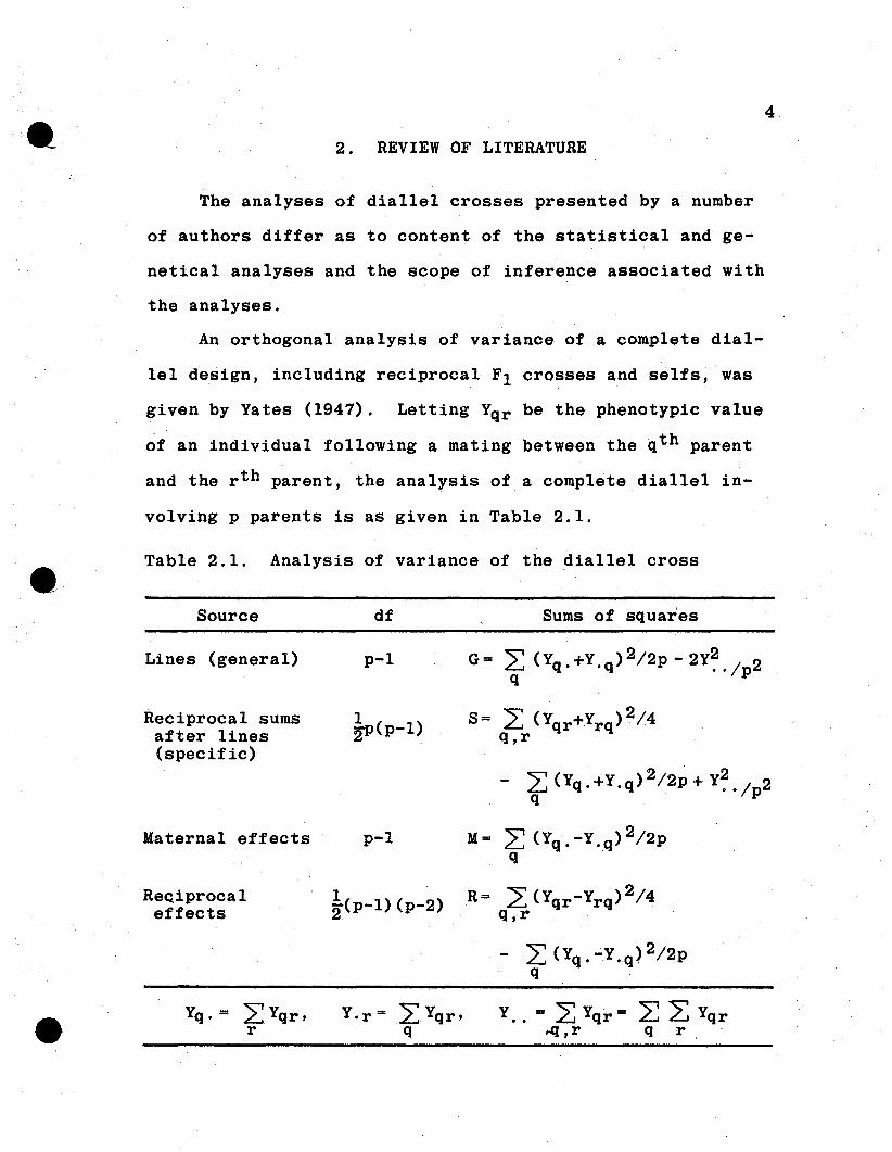
An orthogonal analysis of variance of a complete dial
leI design, including reciprocal Fl crosses and selfs,was
given by Yates (1947). Letting Yqr be the phenotypic value
of an individual following a mating between the qth parent
and the r th parent, the analysis of a complete diallel in-
volving p parents is as given in Table 2.1.
Table 2.1. Analysis of variance of the diallel cross
Source
Lines (general)
Reciprocal sumsafter lines(specific)
Maternal effects
ReGiprocaleffects
Yq • = L.Yqr ,r
df
p-l
p-l
12(p-l) (p-2)
Sums of squares
G= L (yq .+y. q )2/2P - 2Y~./p2q
S= L: (Yqr+Yrq)2/4q,r
- L (Yq . +Y. q)2/2p + Y~ . /p2q
M= ~ (Yq . -Y .q) 2/2pq
R= L (Yqr-Yrq ) 2/4q,r
Y.. = ~ Yqr = ~ 2:: Yqr...q,r q r
5
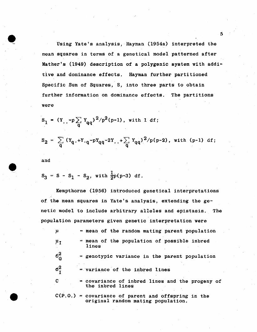
Using Yate's ana1ysis,Hayman (1954a) interpreted the
mean squares in terms of a genetical model patterned after
Mather's (1949) description of a polygenic system with addi-
tive and dominance effects. Hayman further partitioned
Specific Sum of Squares, S, into three parts to obtain
further information on dominance effects. The partitions
were
Sl = (y•. _p~Yqq)2/p2(p_1), with 1 df;q .
and
Kempthorne (1956) introduced genetical interpretations
of the mean squares in Yate's analysis, extending the ge-
netic model to include arbitrary alleles and epistasis. The
population parameters given genetic interpretation were
c
= mean of the random mating parent population
= mean of the population of possible inbredlines
= genotypic variance in the parent population
= variance of the inbred lines
covariance of inbred lines and the progeny ofthe inbred lines
C(P.o.) = covariance of parent and offspring in theoriginal random mating population.
•
6
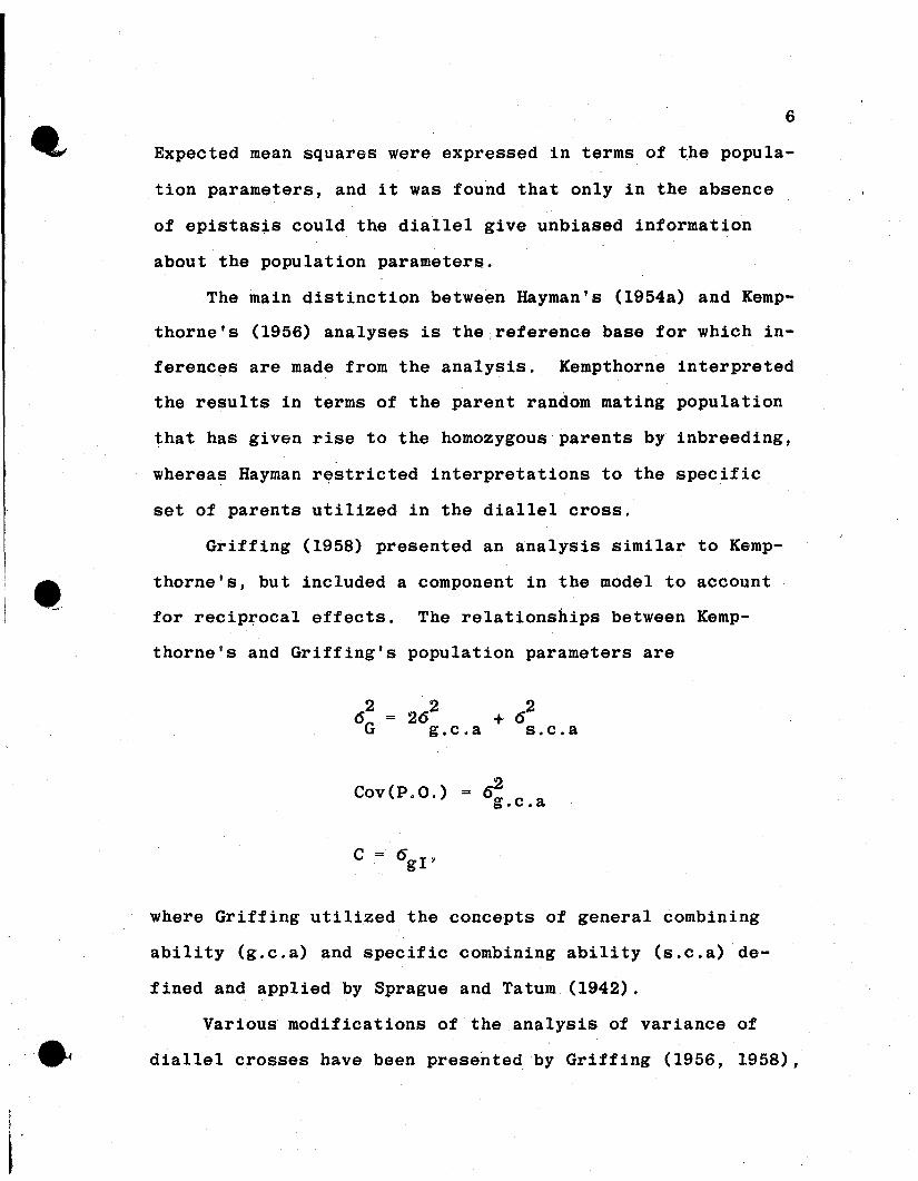
Expected mean squares were expressed in terms of the popula
tion parameters, and it was found that only in the absence
of epistasis could the dial leI give unbiased information
about the population parameters.
The main distinction between Hayman's (1954a) and Kemp
thorne's (1956) analyses is the ,reference base for which in
ferenc~s are made from the analysis. Kempthorne interpreted
the results in terms of the parent random mating population
that has given rise to the homozygous parents by inbreeding,
whereas Hayman r~stricted interpretations to the specific
set of parents utilized in the diallel cross.
Griffing (1958) presented an analysis similar to Kemp-
thorne's, but included a component in the model to account
for recip:r;-ocal effects. The relationships between Kemp-
thorne's and Griffing's population parameters are
+ 62s.c.a
Cov(P.O.) = ~.c.a
where Griffing utilized the concepts of general combining
ability (g.c.a) and specific combining ability (s.c.a) de
fined and applied by Sprague and Tatum (1942).
Various modifications of the analysis of variance of
_ diallel crosses have been presented by Griffing (1956, 1958),
7
Matzinger and Kempthorne (1956), and Cockerham (1963) in
which parents and/or reciprocal matings were excluded from
the analysis.
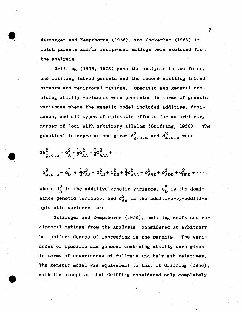
Griffing (1956, 1958) gave the analysis in two forms,
one omitting inbred parents and the second omitting inbred
parents and reciprocal matings. Specific and general com-
bining ability variances were presented in terms of genetic
variances where the genetic model included additive, domi-
nance, and all types of epistatic effects for an arbitrary
number of loci with a~bitrary alleles (Griffing, 1956). The
ti 1 i t t ti . 62 d 62 wgene ca n erprea ons g1ven g.c.a an s.c.aere
where 6~ is the additive genetic variance, 6~ is the domi
nance genetic variance, and 6lA is the additive-by-additive
epistatic variance; etc.
Matzinger and Kempthorne (1956), omitting selfs and re-
ciprocal matings from the analysis, considered an arbitrary
but uniform degree of inbreeding in the parents. The vari-
ances of specific and general combining ability were given
in terms of covariances of full-sib and half-sib relatives.
The genetic model was equivalent to that of Griffing (1956),
with the exception that Griffing considered only completely
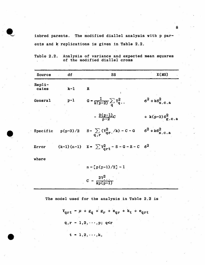
e_.inbred parents. The modified dia11e1 analysis with p par-
ents and k replications is given in Table 2.2.
Table 2.2. Analysis of variance and expected mean squaresof the modified dia11e1 cross
8
Source df SS E(MS)
Repli-cates k-l R
General p-1 G 1 2: y2 2 2=k(p-2) q .. (5 + k6s . c. a
q
_ 2(p-1)C + k(p-2)62p-2 g.c.a
tit Specific p(p-3) /2 S = L; (y2 /k)- C - G 6 2 +k62qr. s.c.aq,r
Error (k-1) (n-1) E= L: y2 - S - G - R - C (52qrt
where
n=[p(p-1)/2] -1
C2Y~ ..
= kp{p-1)
The model used for the analysis in Table 2.2 is
q , r 1 , 2, ... , p; q<r
t = 1,2,···,k,
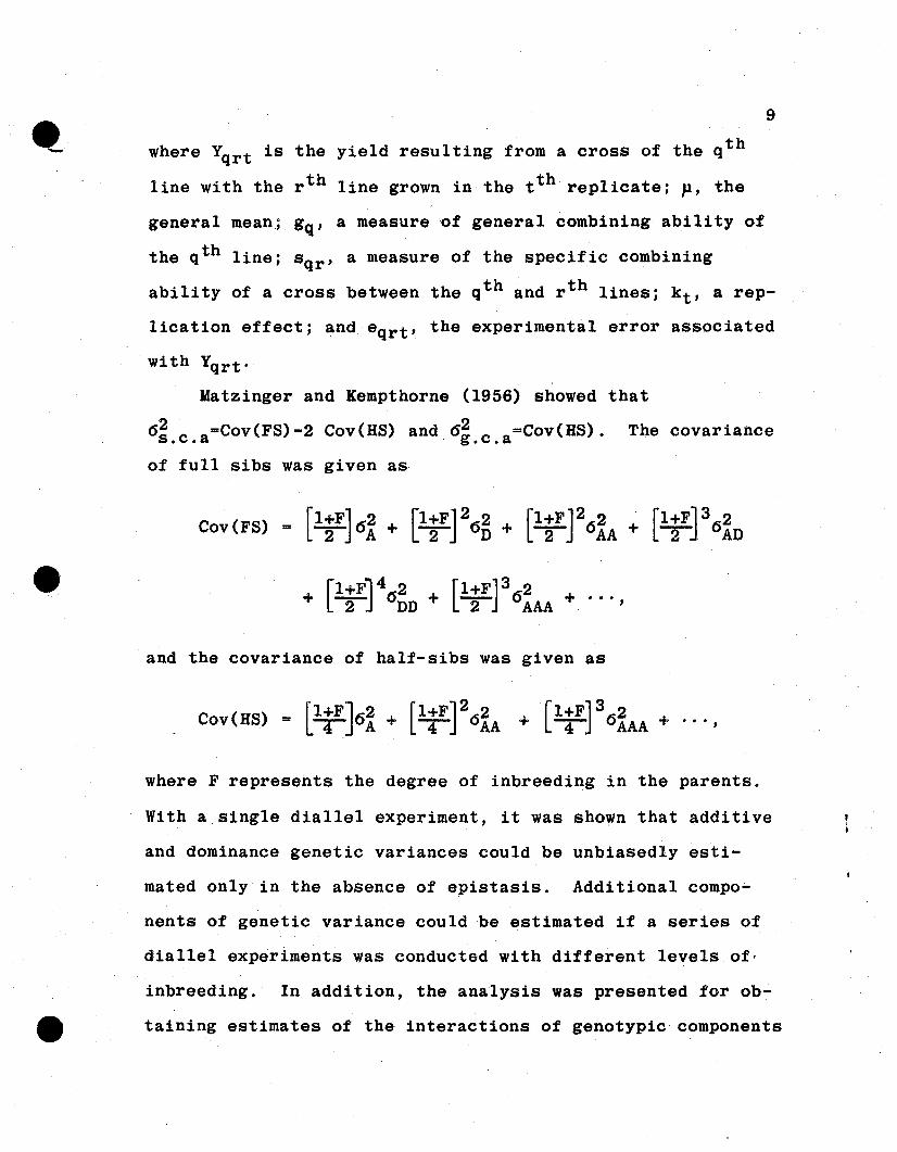
9
yield resulting from a cross of the qth
line grown in the tth replicate; p, the
a measure of general combining ability of
a measure of the specific combining
ability of a cross between the qth and r th lines; kt , a rep
lication effect; andeqrt, the experimental error associated
wi th Yqrt .
Matzinger and Kempthorne (1956) showed that
6~.c.a=COV(FS)-2 Cov(HS) and6:. c . a=COV(HS). The covariance
of full sibs was given as
~ where Yqrt is the
line with the r th
general mean; gq'
the qth line; Sqr'
Cov(FS)
and the covariance of half-sibs was given as
where F represents the degree of inbreeding in the parents.
With a single diallel experiment, it was shown that additive
and dominance genetic variances could be unbiasedly esti-
mated only in the absence of epistasis. Additional compo-
nents of genetic variance could be estimated if a series of
diallel experiments was conducted with different levels of·
inbreeding. In addition, the analysis was presented for ob-
taining estimates of the interactions of genotypic components
e'-10
of variance with environments represented by locations and
ye~rs.
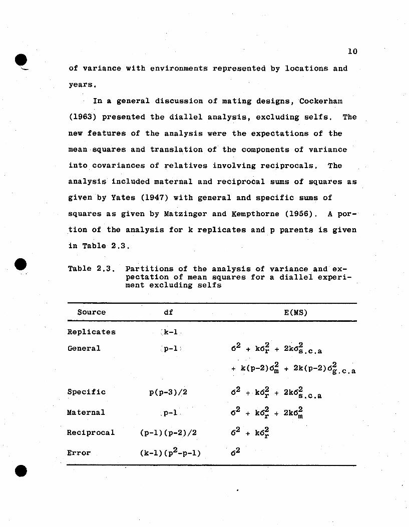
In a general discussion of mating designs,Cockerham
(1963) presented the diallel analysis, excluding selfs. The
new features of the analysis were the expectations of the
mean squares and translation of the components of variance
into covariances of relatives involving reciprocals. The
analysis included maternal and reciprocal sums of squares as
given by Yates (1947) with general and specific sums of
squares as given by Matzinger and Kempthorne (1956). A por-
tion of the analysis for k replicates and p parents is given
in Table 2.3.
Table 2.3. Partitions of the analysis of variance and expectation of mean squares for a diallel experiment excluding selfs
Source
Replicates
General
Specific
Maternal
Reciprocal
Error
df
:k-l ..
:p-l~
p(p-3)/2
,p-l
(p-l) (p-2)/2
(k-l) (p2_p_l )
E(MS)
62 + k6~ + 2k6~.c.a
+ k(p-2)6~ + 2k(P-2)6~.c.a
62 + k62 2r + 2k6s . c . a
6 2 + k62 + 2kCS;r
62 + k62r
6 2
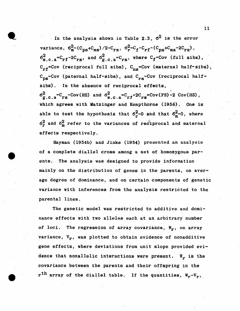
11
In the analysis shown in Table 2.3, 62 is the error
variance, 6;= (Cps+Cms) 12-Crs ' (5~=Cf-Crf- (Cps+Cms-2Crs)"
6~.c.a=Crf-2Crs' and 6:. c . a=Crs ' where Cf=Cov (full sibs),
C f=CoV (reciprocal full sibs), C =Cov (maternal half-sibs),r ms.
Cps=Cov (paternal half-sibs), and Crs=Cov (reciprocal half-
sibs). In the absence of reciprocal effects,
(52 =C =Cov(HS) and 62 =C -2C =COV(FS):2 Cov(HS),g.c.a rs s.c.a rf rswhich agrees with Matzinger and Kempthbrne (1956). One is
able to test the hypothesis that 6~=O and that 6~=O, where
6~ and 6; refer to the variances of red(iprocal and maternal
effects respectively.
Hayman (1954b) and Jinks (1954) presented an analysis
of a complete dialle1 cross among a set of homozygous par-
ents. The analysis was designed to provide information
mainly on the distribution of genes in the parents, on aver-
age degree of dominance, and on certain components of genetic
variance with inferences from the analysis restricted to the
parental lines.
The genetic model was restricted ~o additive and domi-
nance effects with two alleles each at an arbitrary number
of loci. The regression of array covariance, Wr , on array
variance, Vr , was plotted to obtain evidence of nonadditive
gene effects, where deviations from unit slope provided evi-
dence that nonallelic interactions were present. Wr is the
covariance between the parents and their offspring in the
r th array of the diallel table. If the quantities, Wr-Vr ,
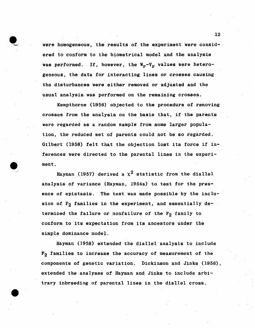
12
were homogeneous, the results of the experiment were consid
ered to conform to the biometrical model and the analysis
was performed. If, however, the Wr-Vr values were hetero
geneous, the data for interacting lines or crosses causing
the disturbances were either removed or adjusted and the
usual analysis was performed on the remaining crosses.
Kempthorne (1956) objected to the procedure of removing
crosses from the analysis on the basis that, if the parents
were regarded as a random sample from some larger popula-
tion, the reduced set of parents could not be so regarded.
Gilbert (1958) felt that the objection lost its force if in-
ferences were directed to the parental lines in the experi-
ment.
Hayman (1957) derived aX2 statistic from the diallel
analysis of variance (Hayman, 1954a) to test for the pres
ence of epistasis. The test was made possible by the inclu-
sion of F2 families in the experiment, and essentially de
termined the failure or nonfailure of the F2 family to
conform to its expectation from its ancestors under the
simple dominance model.
Hayman (1958) extended the dialleloanalysis to include
F2 families to increase the accuracy of measurement of the
components of genetic variation. Dickinson and Jinks (1956),
extended the analyses of Hayman and Jinks to include arbi-
trary inbreeding of parental lines in the diallel cross.
e\.~_ .../
13
Hayman (1960) attempted to relate the main lines of ap-
proach to analyzing and interpreting the diallel cross. In
so doing, he considered the homozygous parents as a random
sample from an inbred but originally random mating popula-
tion. Population parameters were translated into components
of genetic variances defined by Hayman (1954b), and the
population parameters were related to those given by Kemp-
thorne (1956) and Griffing (1958). Hayman then provided a
set of unbiased estimators and a set of maximum likelihood
estimators from the dial1el analysis for the population pa-
rameters. The variance-covariance matrix of the unbiased
estimators for population parameters and genetic components
was given, where variances and covariances of the quadratic
functions were derived under the assumption of normally dis
tributed effects in the model. From the nature of the vari-
ances, it was suggested that at least 10 parents should be
used if the dia11e1 cross was to provide useful estimators
of the population parameters.
Considering the interpretation of the genetic param
eters defined by Hayman (1954b) £or a fixed set of lines,
one might ask whether or not these parameters more appropri-
ate1y apply to a random mating population defined by the
gene frequencies of the set of lines. If the parameters are
appropriate ~or such a population, there is an error of in-
ference associated with estimators of the parameters. To
make inferences to a reference population, an adequate
14
genetic sampling plan is necessary to determine the error of
inference.
In the following sections, an attempt is made to pro
vide estimators and their associated errors from a diallel
analysis for genetic variances of the random mating popula
tion derived from the set of completely inbred parents used
for the diallel mating.
e'''... /
15
3. SAMPLING DISTRIBUTIONS
The sampling variables used in the·solution of this
problem and their probability distributions can be illus
trated by initially considering a random mating diploid
population in linkage equilibrium consisting of genotypes
having m loci, each with two alleles (Band b). The alleles
is imposed on the random mating population, such that Pi
does· not change ,. to form a completely inbred population of
homozygous geno1:.ypes. The frequency of the genotypes, BB
and bb, at the i th locus in the inbred population will be Pi
and (l~Pi)' respectively.
Let X={1,2" .. ,m} be the set of m loci. A homozygous
genotype in the population is completely defined by specify
.ing the set of loci, eJthat has the positive alleles, BB,
since the remainder of the loci, ~~-~, must have the nega
tive alleles, bb. For example, with two loci, ~={1,2)
specifies the genotype BI BI B2B2 , a={21 specifies the geno
type bl b l B2B2 , etc. Thus all possible homozygous genotypes
for the m loci are specified by considering all possible
subsets of X, including the empty set, ~=g, and the complete
set, a=4C. The relative frequency of a genotype in the in-
bred population is given by
16
(3.1)
Let X(a) denote the number of lines having genotype a
in a particular random sample of inbred lines. The geno
typic composition of a particular sample of n lines from the
-inbred population is specified by the X(~)'s for that sample
where
= n. (3,2)
If welet ~i=\aliea}, !,~" ~i is the set of all a contain
ing the i th locus, the number of lines in the ~ample.that
contains the set of positive alleles, BB, at the i th locus
is
Yi = L X(a).aC'~i .
(3.3)
Conversely, the number of lines in the sample that contain
the negative alleles, bb, at thei th locus is n-Yi' The
relative frequency of the B allele at the i th locus in the
sample is given by
(3.4)
and the frequency of the b allele is I-Pi~
. Likewise, letting ~ij={al(i,j)£a~, the number of lines
in the sample containing the set of positive alleles, BB, at
both the i th and jth loci is
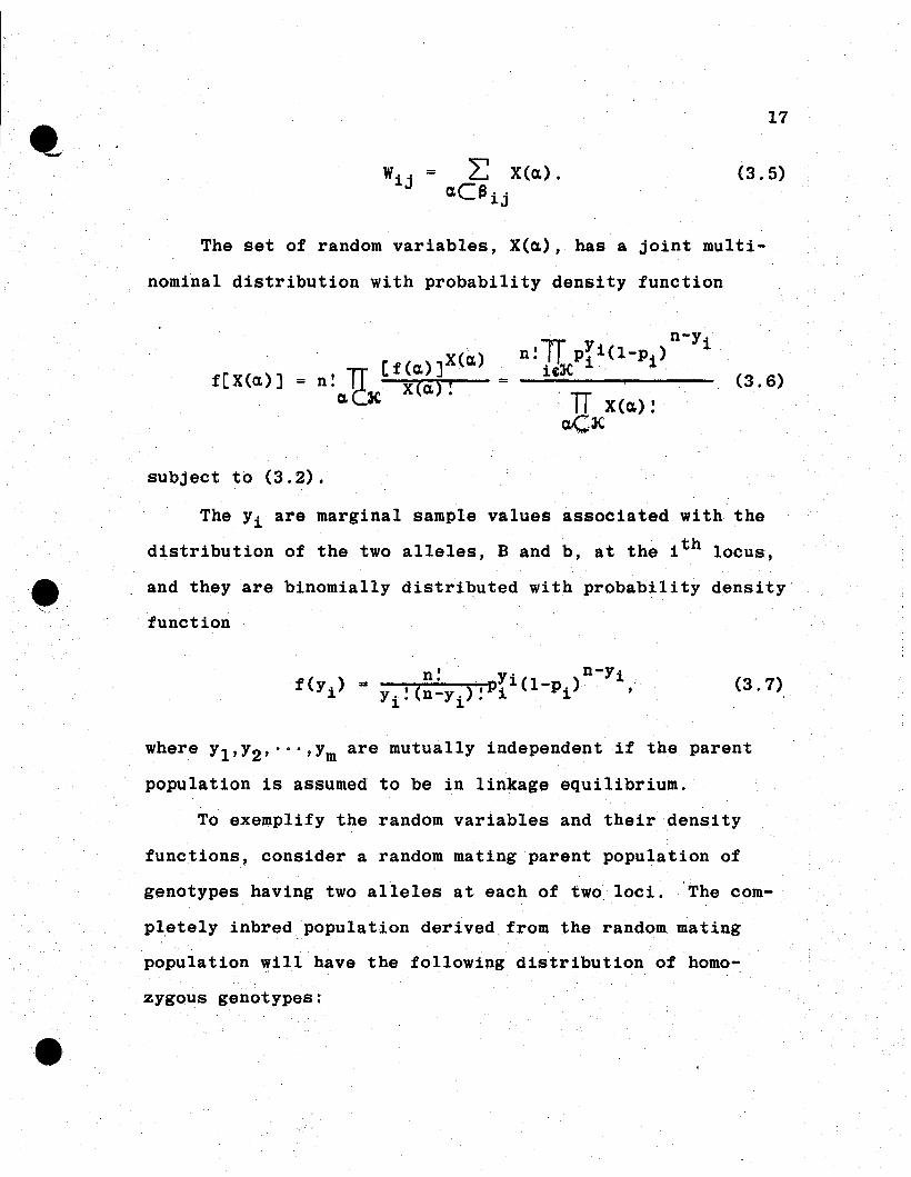
17
(3.5)
The set of random variables, X(~), has a joint mu1ti
nominal distribution with probability density function
f[X(a.)] =
n-yn:11 pYi(l-p.) i
ide i 1
. TT X(~)!
a.CK
(3.6)
subject to (3.2).
The Y1 are marginal sample values associated with the
distribution of the two alleles, Band b, at the i th locus,
and they are binomially distributed with probability density'
function
(3.7)
where YI'Y2'···'Ym are mutually independent if the parent
population is assumed to be in linkage equilibrium.
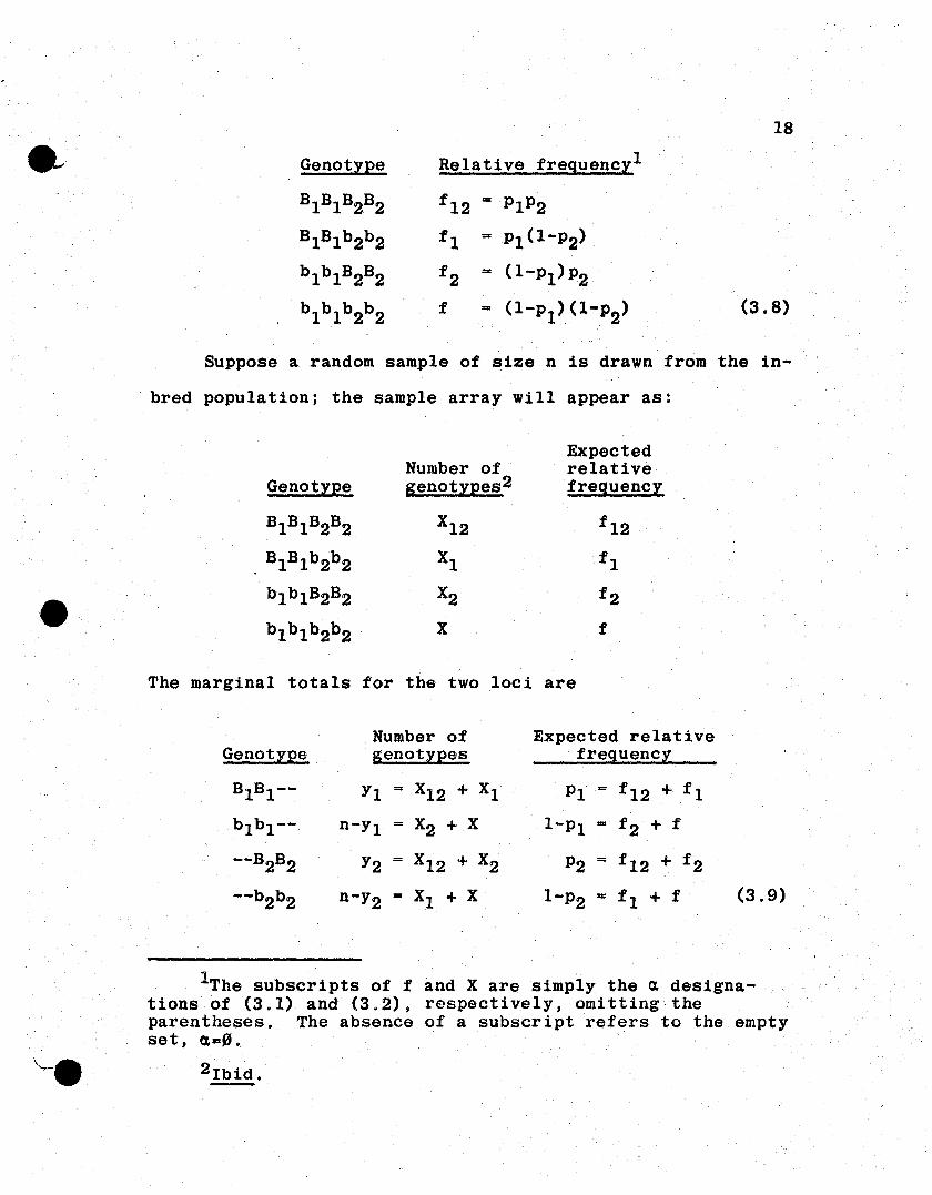
To exemplify the random variables and their density
functions, consider a random mating parent population of
genotypes having two alleles at each of two loci. The com-
pletely inbred population derived from the random mating
population w.ill have the following distribution of homo
zygous genotypes:
Genotype
Bl Bl B2B2
B1Bl b2b2
b l b l B2B2
b l b1b2b2
Relative frequencyl
f 12 = PlP2
f l = Pl{1-P2)
f 2 = (1-Pl)P2
f ... (1-Pl)(1-P2)
18
(3.8)
Suppose a random sample of size n is drawn from the in-
bred population; the sample array will appear as:
ExpectedNumber of relative
Genotype genotypes2 frequency
Bl B1B2B2 X12 f 12
Bl B1b2b2 Xl f l
b1blB2B2 X2 f 2
b1b1b2b2 X f
The marginal totals for the two loci are
Number of Expected relativeGenotype genotypes frequency
BlBl -- Yl = X12 + Xl PI = f 12 + f 1
b1b1-- n-Yl = X2 + X I-PI f 2 + f
--B2B2 Y2 X12 + X2 P2 = f 12 + f 2
--b2b2 n-Y2 = Xl + X I-P2 ... f 1 + f (3.9)
IThe subscripts of f and X are simplythe ~ designations of (3.1) and (3.2), respectively, omitting theparentheses. The absence of a subscript refers to the emptyset, 0.=0.
2Ibid.
•
19
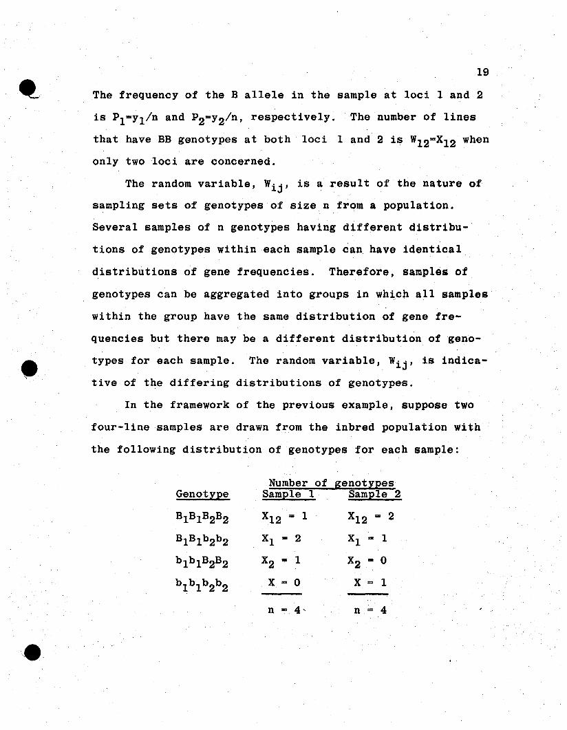
The frequency of the B allele in the sample at loci 1 and 2
is Pl=yl/n and P2=Y2/n, respectively. The number of lines
that have BB genotypes at both loci 1 and 2 isW12""X12 when
only two loci are concerned.
The random variable, Wij , is a result of the nature of
sampling sets of genotypes of size n from a population.
Several samples of n genotypes having different distribu
tions of genotypes within each sample can have identical
distributions of gene frequencies. Therefore, samples of
genotypes can be aggregated into groups in which all samples
within the group have the same distribution of gene fre
quencies but there may be a different distribution ofgeno-
types for each sample. The random variable, Wij , is indica
tive of the differing distributions of genotypes.
In the framework of the previous example, suppose two
four-line samples are drawn from the inbred population with
the following distribution of genotypes for each sample:
Number of genotypesGenotype Sample I Sample 2
Bl Bl B2B2 Xl2 == I Xl2 == 2
BIBl b2b2 Xl 2 Xl == 1
bl b l B2B2 X2 1 X2 == 0
bl b1b2b2 X "" 0 X == 1
n "" 4, n == 4
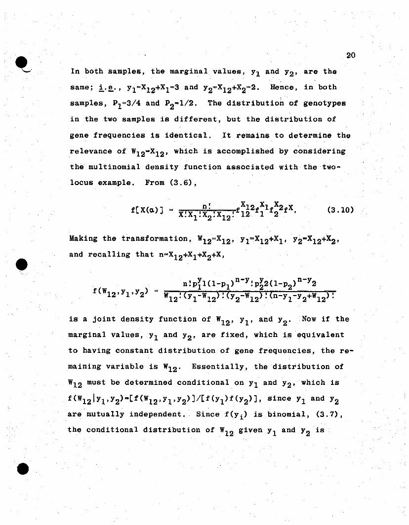
20
In both samples, the marginal values, Yl and Y2' are the
same; !..!.., Yl=X12+Xl -3 and Y2=X12+X2=2. Hence, in both
samples, PI=3/4 and P2=1/2. The distribution of genotypes
in the two samples is different, but the distribution of
gene frequencies is identical. It remains to determine the
,relevance of W12=X12 , which is accomplished by considering
the multinomial density function associated with the two
locus example. From (3.6),
f[X(a.)] n! X12 Xl X2 X= X'X 'X 'X IfI2 f l f 2 f. 1· 2· 12· -
(3.10)
Making the transformation, W12=XI2 , YI=X12+X1 , Y2=X12+X2 ,
and recalling that n=XI2+Xl +X2+X,
is a joint density function of W12 , Y1' and Y2 . Now if the
marginal values, Y1 and Y2' are fixed, which is equivalent
to having constant distribution of gene frequencies, the re-
maining variable is W12 . Essentially, the distribution of
W12 must be determined conditional on Yl and Y2' which is
f(W12 !Yl'Y2)=[f(W12 'Yl'Y2)]/[f(Yl)f(Y2)]' since Yl and Y2
are mutually independent. Since f(Yi) is binomial, (3.7),
the conditional distribution. of W12 given Yl and J2 is
21
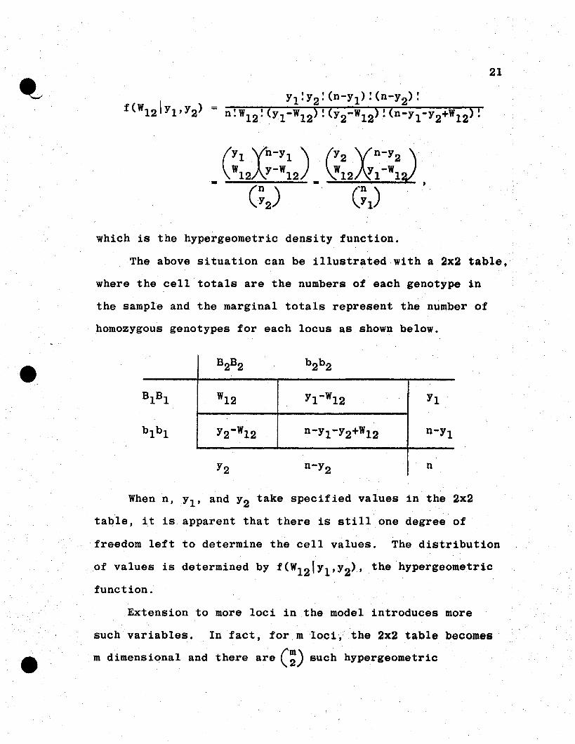
Y1: Y2:(n-Y1):(n-Y2):f(W12 IYl'Y2) = n:w12:<Y1-W12>:<Y2-W12>:<n-YI-Y2+W12):
which is the hypergeometric density function.
The above situation can be illustrated with a 2x2 table,
where the cell totals are the numbers of each genotype in
the sample and the marginal totals represent the number of
homozygous genotypes for each locus as shown below.
B2B2 b2b2
BIBI W12 YI-W12 Yl
blbl Y2-W12 n-YI-Y2+W12 n-Yl
Y2 n-Y2 n
When n, Yl' and Y2 take specified values in the 2x2
table, it is apparent that there is still one degree of
freedom left to determine the cell values. The distribution
of values is determined by f(W12 \Y1'Y2)' the hypergeometric
function.
Extension to more loci in the model introduces more
such variables. In fact, for m 10.ci, the 2x2 table becomes
m dimensional and there are C;) such hypergeometric
22
variables; !.~., one hypergeometric variable, Wij' for each
pair of loci.
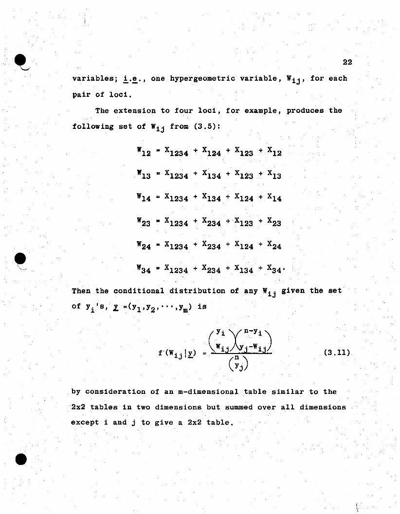
The extension to four loci, for example, produces the
following set of Wij from (3.5):
Then the conditional distribution of any Wij given the set
of Yi's, 1. =(Yl'Y2,""Ym) is
(3.11)
by consideration of an m-dimensional table similar to the
2x2 tables in two dimensions but summed over all dimensions
except i and j to give a 2x2 table.
iI.I
23
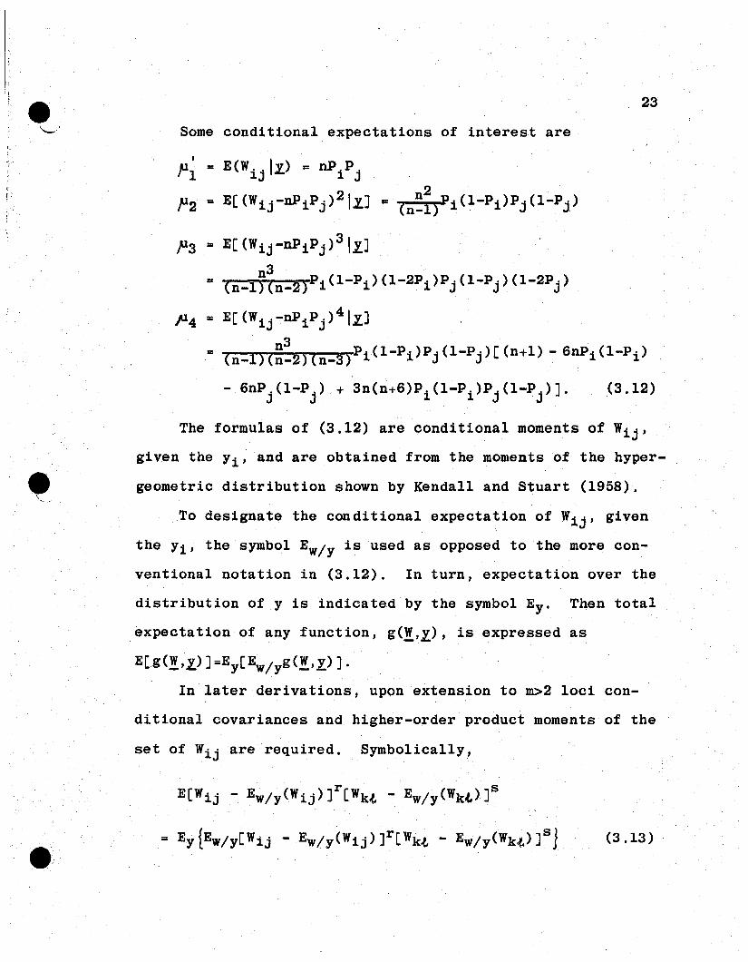
Some conditional expectations of interest are
F~ = E(Wijl~) = nPiPj
f2 = E[(Wij-nPiPj)21~J
F3 = E[(Wij-nP i Pj)3IzJ
n3= (n-l) (n-2)Pi (l-Pi ) (l-2Pi )Pj (l-Pj ) (1-2Pj )
P4 = E[(Wij -nPi Pj )4IzJ
= (n-l) (~:2) (n-3)Pi (l-Pi)Pj (l-Pj )[ (n+l) - 6nPi (l-Pi )
- 6nPj (l-Pj ) + 3n(n+6)Pi (l-Pi )Pj (1-Pj )]. (3.12)
The formulas of (3.12) are conditional moments of Wij '
given the Yi' and are obtained from the moments of the hyper
geometric distribution shown by Kendall and Stuart (1958).
To designate the conditional expectation of Wij' given
the Yi' the symbol Ew/ y is used as opposed to the more con
ventional notation in (3.12). In turn, expectation over the
distribution of y is indicated by the symbol Ey . Then total
expectation of any function, g(W,Z), is expressed as
E[g(W,y)]=Ey[EW/yg(W,.l)].
In later derivations, upon extension to m>2loci con-
ditional covariances and higher-order product moments of the
set of Wij are required. Symbolically,
(3.13 )
,-. ,.-. :,,'
24
til. must be determined for r,s=1,2 and j~t, where i and k may
or may not be equal.
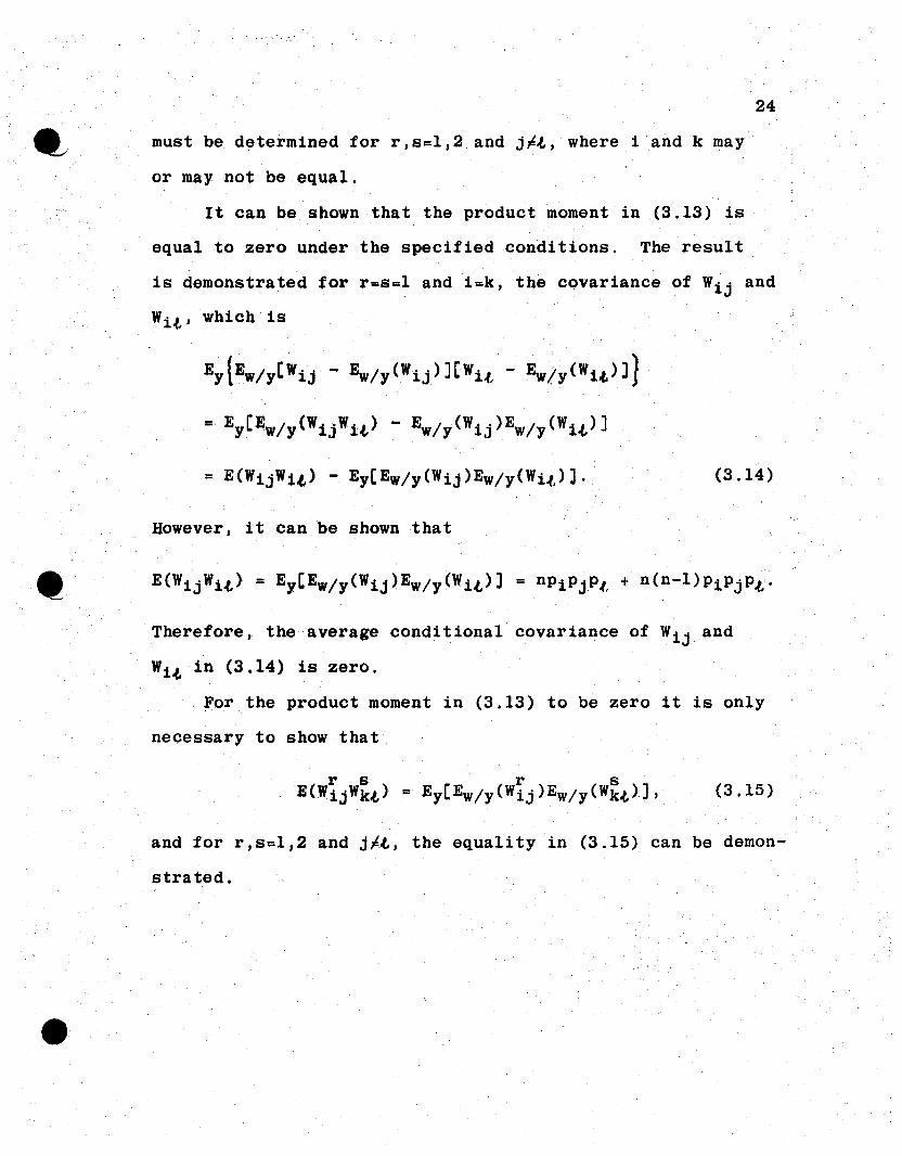
It can be shown that the product moment in (3.13) is
equal to zero under the specified conditions. The result
is demonstrated for r=s=l and i=k, the covariance of Wij and
Wit' which is
(3.14)
However, it can be shown that
Therefore, the average conditional covariance of Wijand
Wit in (3.14) is zero.
For the product moment in (3.13) to be zero it is only
necessary to show that.
(3.15)
and for r,s=l,2 and jtt, the equality in (3.15) can be demon-
strated.
25
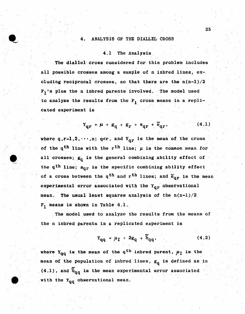
4. ANALYSIS OF THE DIALLEL CROSS
4.1 The Analysis
The dial leI cross considered for this problem includes
all possible crosses among a sample of n inbred lines, ex-
eluding reciprocal crosses, so that there are the n(n-l)/2
Fl'S plus the n inbred parents involved. The model used
to analy~ethe results from the Fl cross means in a repli
cated experiment is
(4.1)
(4.2)
where Yqq is the mean of the qth inbred parent, PI is the
mean of the population of inbred lines, gq is defined as in
(4.1), and ~qq is the mean experimental error associated
with the Yqq observational mean.
26
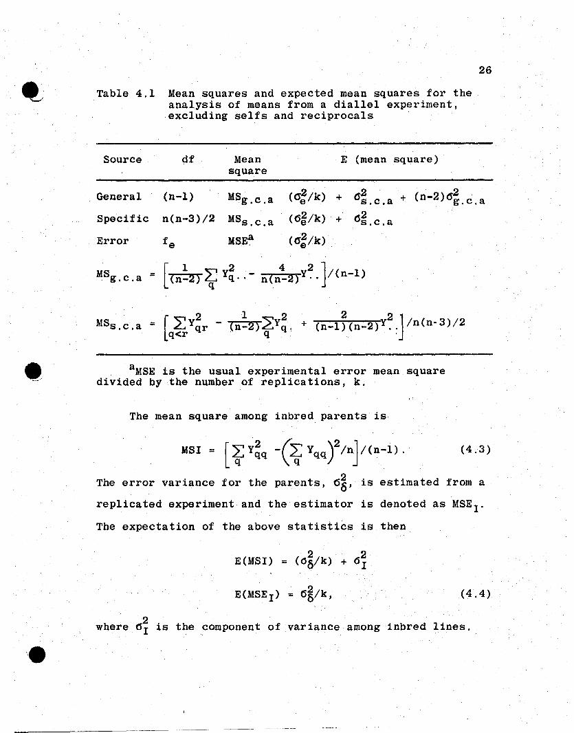
Table 4.1 Mean squares and expected mean squares for theanalysis of means from a dial leI experiment,excluding selfs and reciprocals
Source df Meansquare
E (mean square)
General (n-l) MSg . c .a «5~/k) + 6'2 + (n-2)0'~.c.as.c.a
Specific n(n-3)/2 MSs . c . a (6~/k) + (52s.c.a
Error f e MSE~ (O'~/k)
MS. g.c.a
MSs •c . a[
2 1 2 2 2]= 2;Yqr - (n-2)L:Yq , + (n-l) (n-2)Y., /n(n-3)/2q<r . q .
aMSE is the usual experimental error mean squaredivided by the number of replications, k.
The mean square among inbred parents is
MSI = [~Y~q -(2.tYqqY/n}(n-l). (4.3)
The error variance for the parents, 6~, is estimated from a
replicated experiment and the estimator is denoted as MSE!,
The expectation of the above statistics is then
E(MSI) = (O~/k) + 6~
E(MSE1) = e>g/k, (4,4)
where 6i is the component of variance among inbred lines.
', .. .r
27
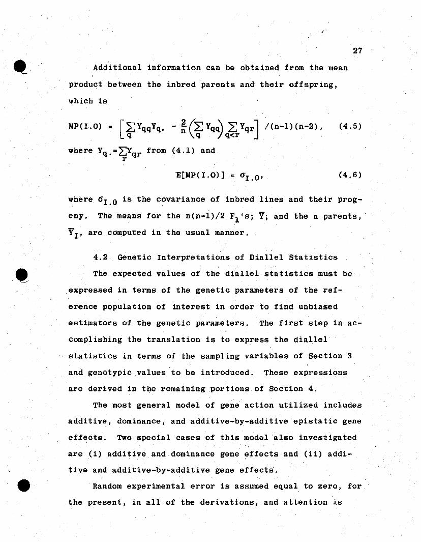
Additional information can be obtained from the mean
product between the inbred parents and their offspring,
which is
loIP(l.O) = [~YqqYq. - ~(tYq~q~/qrJ !(n-l)(n-2),
where Yq.=~Yqr from (4.1) andr
E[MP(I.O)] = aI.O'
(4.5)
(4.6)
where 61 . 0 is the covariance of inbred line$ and their prog
eny. The means for the n(n-l)/2 Fl's; Yj and the n parents,
YI , are computed in the usual manner.
4.2 Genetic Interpretations of Diallel Statistics
The expected values of the diallel statistics must be
expressed in terms of the genetic parameters of the ref-
erence population of interest in order to find unbiased
estimators of the genetic parameters. The first step in ac
complishing the translation is to express the diallel
statistics in terms of the sampling variables of Section 3
and genotypic values to be introduced. These expressions
are derived in the remaining portions of Section 4.
The most general model of gene action utilized includes
additive, dominance, and additive-by-additive epistatic gene
effects. Two special cases of this model also investigated
are .(i) additive and dominance gene effects and (ii) addi
tive and additive-by-additive gene effects.
Random experimental error is assumed equal to zero, for
the present, in all of the derivations, and attention is
28
focused on the genetic components of interest. Even though
random error is not included in the model, the mean squares
and products are referred to as diallel statistics in
Sections 4 and 5. The consequences of adding random experi-
mental error to the model are taken up in Section 6.
The mean squares and products computed for the diallel
analysis, expressed in terms of sampling variables and
genotypic values, are illustrated for two loci. All pos
sible crosses among the n inbred parents sampled at random
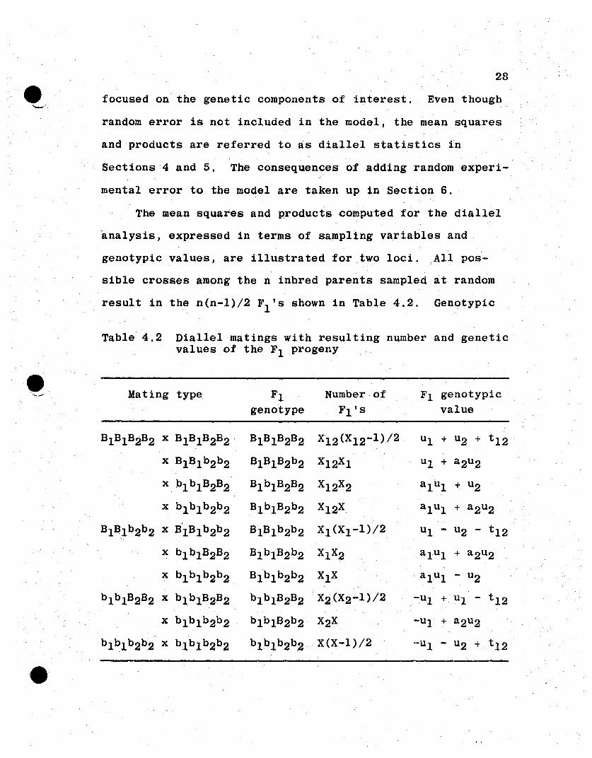
result in the n(n-l)/2 FIts shown in Table 4.2. Genotypic
Table 4.2 Diallel matings with resulting number and geneticvalues of the Fl progeny
e Mating type Fl Number of Fl genotypic'-../
genotype FIts value
Bl Bl B2B2 x BI BI B2B2 · BIBlB2B2 X12(X12-l )/2 ul + u2 + t 12
x BI Bl b2b2 BIBIB2b2 XI2Xl ul + a2u2
x Pl bI B2B2 Bl bIB2B2 X12X2 alul + u2
x bl bl b2b2 B1bI B2b2 X12X alul + a2u2
BIal b2b2 x B'lBIb2b2 BIBIb2b2 Xl(Xl-I)/2 ul - u2 - t 12
x b1b1B2B2 BI b1B2b2 XI X2 alul + a2u2
x b1b1b2b2 Bl bl b2b2 XIX alul - u2
bl bl B2B2 x b1blB2B2 bl bl B2B2 X2(X2-l )/2 -ul + ul - t 12
x blblb2b2 blbIB2b2 X2X -ul + a2u2
bI b1b2b2 x blblb2b2 b1b1b2b2 X(X-l)/2 -ul - u2 + t12
,e
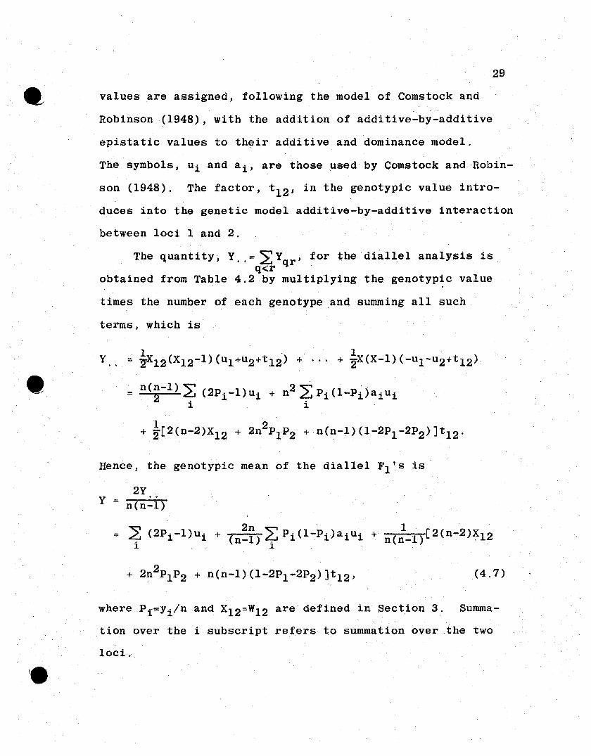
•29
values are assigned, following the model of Comstock and
Robinson (1948), with the addition of additive-by-additive
epistatic values to their additive and dominance model,
The symbols, ui and ai' are those used by Comstock and Robin
son (1948), The factor, t 12 , in the genotypic value intro
duces into the genetic model additive-by-additive interaction
between loci 1 and 2.
The quantity, Y,.::: 2 Yqr I for the' diallel analysis isq<r
obtained from Table 4.2 by multiplying the genotypic value
times the number of each genotype and summing all such
terms, which is
•Y
1 . 1 .::: ~X12(X12-1)(ul+u2+t12) + ... + 2X(X-l)(-ul-u2+ t 12)
= n(~-l) ~ (2Pi -l)ui + n2 L: Pi (l-Pj.>aiui1 i
Hence, the genotypic mean of the diallel FIls is
2YY ::: n(n-l)
where Pf""Yi/n and X12=W12 are defined in Section 3. Summa
tionover the i subscript refers- to summation over the two
loci.
30
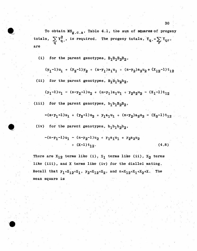
To obtain MSg .c. a' Table 4.1, the sum of squares of progeny
totals, L y2 , is required . The progeny totals, Yq . =2: Yqr ,q q. r
are
-(n-YI-I)ul - (n-Y2-l )u2 + Ylalul + Y2a 2u2
+ (X-l)t12 · (4.8)
There are X12 terms like (i), Xl terms like (ii),X2 terms
like (iii), and X terms like (iv) for the diallel mating.
Recall that YI=XI2+X I , Y2=XI2+X2 , and n=X12+XI +X2+X. The
mean square is
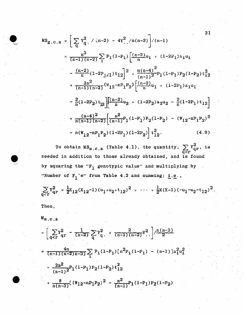
31e',-, MSg . c . a · [i?:. /in-2) - 4Y~ /n Cn-2)}C n- 1 )
= n3 L Pi (I-Pi) [(n-2)Ui + (1-2Pi)ai ui
(n-I)(n-2) i l n
2(n-2) J2 n(n-4) , 2
n (1-2P j /l)t12, + (n-l)2 Pl(1-Pl)P2(1-P2)tI 2
2n2(rn P p >[(n-2)
+ (n-I)(n-2} "12-n 1 2' n uI+ (1-2PI)aIul
(4.9)
Then,
Ms.c.a
= [ ",",y2 I ,",y2 2 y2 ]/n(n-3)q-zr qr - (n-2) ~ q. + (n-I) (n-2) .. 2
32
+ (n_l)(n~2)(n_3)1~(W12-nPiPj)[(n-l) - n2Pi(1-Pi)]aiuit12
+'n(n-l)(n~2)(n-3)t(n2-3n+4)[(W12-nPlP2)2
n2- (n~1)Pl(l-Pl)P2(1-P2)]
- 2n(n-l)(W12-nPlP2)(l-2Pl)(1-2P2)Jt~2' (4.10)
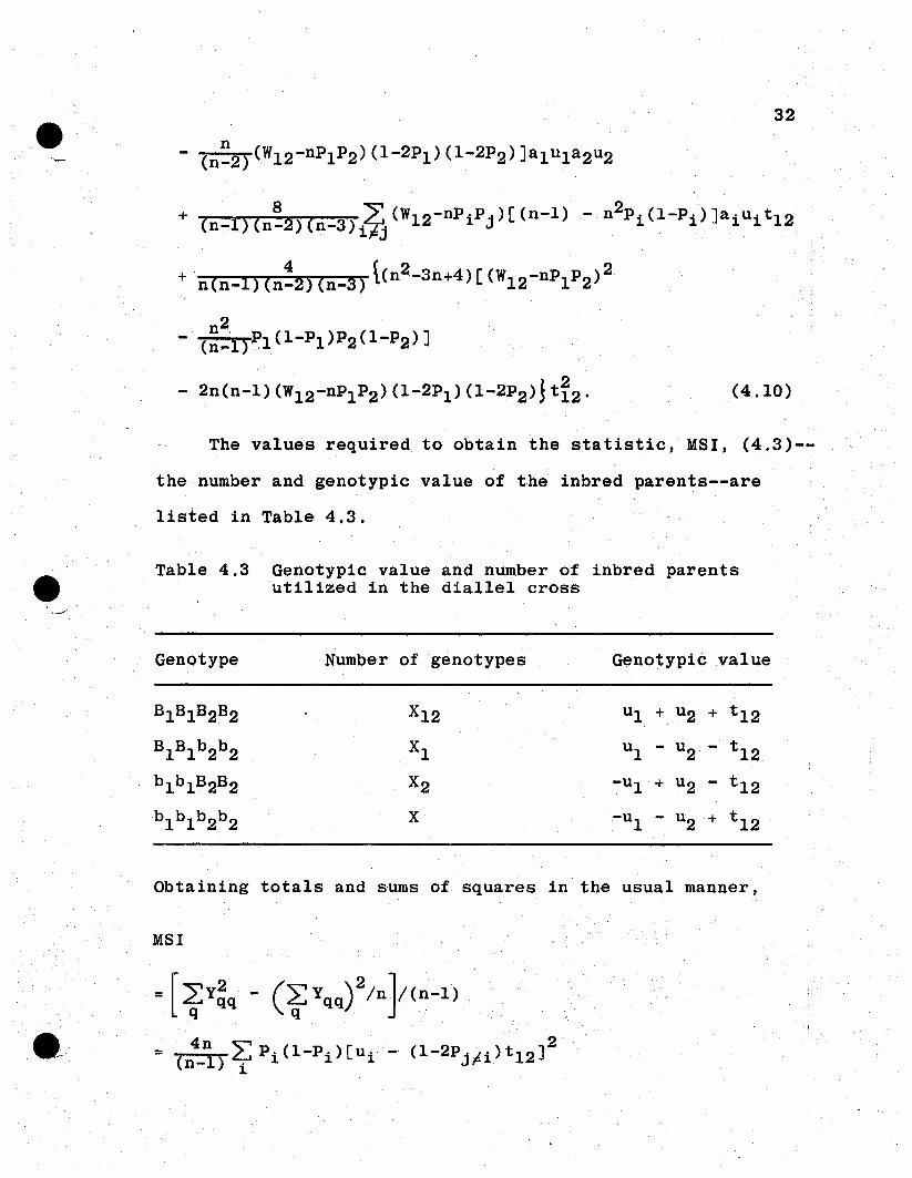
e-,
The values required to obtain the statistic, MSI, (4.3)--
the number and genotypic value of the inbred parents--are
listed in Table 4.3.
Table 4.3 Genotypic value and number of inbred parentsutilized in the diallel cross
Genotype Number of genotypes Genotypic value
Bl Bl B2B2 X12 ul + u2 + t 12
Bl Bl b2b2 Xl ul - u2 - t 12bl bl B2B2 X2 -ul + u2 - t 12
b l bl
b 2b 2 X -ul - u2 + t 12
Obtaining totals and sums of squares in the usual manner,
MSI
=[tY~q - (t: yqq)2/n}(n-l)
= 4n 2:;P.(l-P.)[u, - (1-2PJ'1i)t12 J2
(n-l) i ~ ~ ~ F
+ 1~:~~~§)Pl(1-Pl)P2(1-P2)t~2 + (n~1)(W12-nPIP2)[UIU2
+ (1-2Pl )ul t12 + (1-2P2)u2t 12 - (1-2Pl)(1-2P2)t~2J
16 [ n2 2J. 2+ n(n-l) L(n-1)P1 (1-P1)P2(1-P2) - (W12-nP1P2) t 12 •
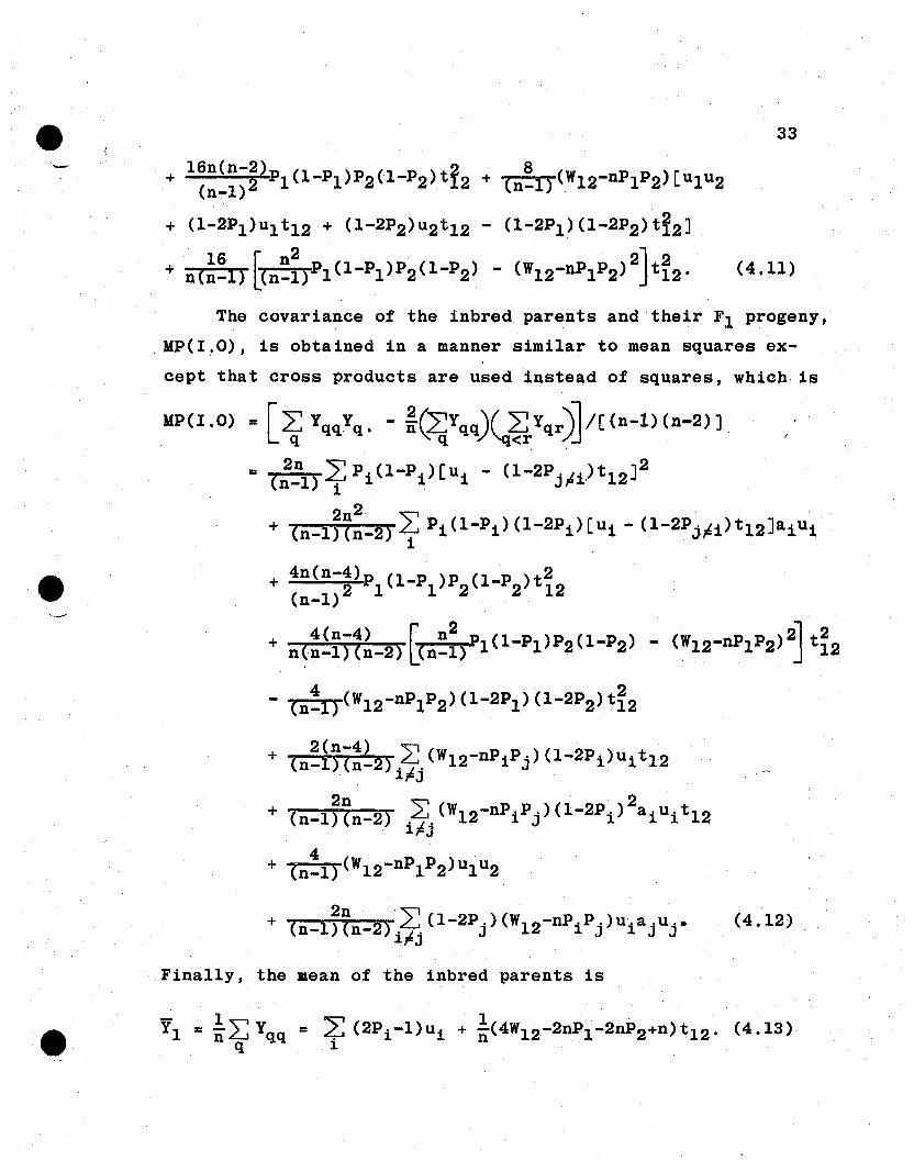
33
(4.11)
The covariance of the inbred parents and their Fl progeny,
,MP(I.O), is obtained in a manner similar to mean squares ex
cept that cross products are used instead of squares, which is
1oIP(I,O) = [ i?qqYq • - ~~Yq.v~~Yqr)] j[(n-l)(n-2)]
II (:~l) t: Pi(l-Pi ) CUi - (1-2Pj~i'>t12J2
2n2 ""V+ (n-1) (n-2) L..J Pi (l-Pi ) (1-2Pi ) [ui - (1-2Pj~i) t 12Jaiui
i
+ 4n(n-4)p (l-P )P (1-P )t2(n_l)2 1 1 2 2 12
+ n(::~)t~-2) [(n~~)Pl (1-Pl)P2(1-Pa) - (W12-nP1P2)~ t~2
4 2- (n_lY(W12-nP1P2)(1-2P1)(1-2P2)t12
2(n-4) ~ ( ( ,+ (n-l)(n-2)~ W12-nPi P j ) 1-2Pi )ui t 12
2n ~ 2+ (n-l)(n-2) ~(W12-nPiPj)(1-2Pi) a i ui t 12
4+ (n_l)(W12-nPlP2)ulu2
·2n ~+ ( 1)( 2) LJ (1-2P.)(W12-nP1·P.)u·.a .u .•n- n- i~j J J 1 J J
Finally, the mean of the inbred parents is
(4.12)
34
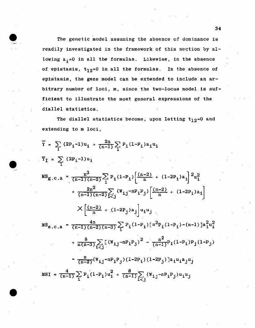
The genetic model assuming the absence of dominance is
readily investigated in the framework of this section by al-
lowing ai=O in all the formulas. Likewise, in the absence
of epistasis, t 12 =O in all the formulas. In the absence of
epistasis, the gene model can be extended to include an ar-
bitrary number of loci, m, since the two-locus model· is suf-
~icient to illustrate the most general expressions of the
diallel statistics.
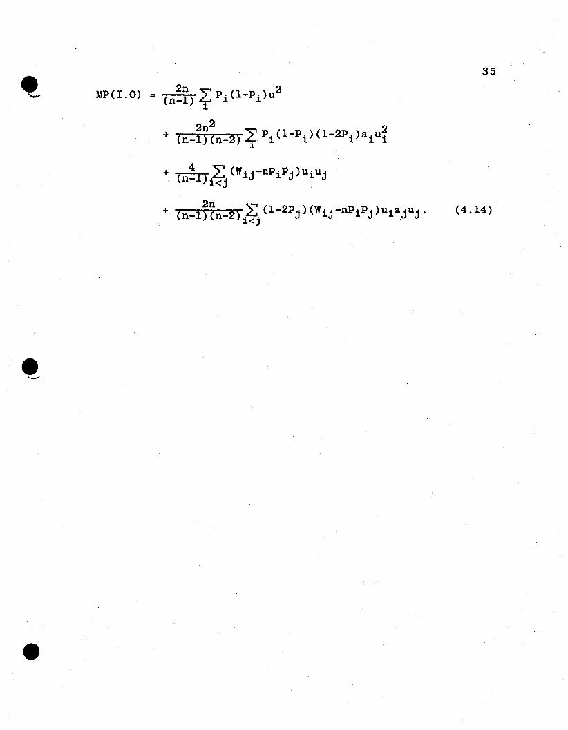
The diallel statistics become, upon letting tl2=O and
extending to m loci,
YI = ~ (2Pi-l )ui
n3 ~ r,(n-2) ] 2 2MSg . c . a =. (n-l) (n-2) t Pi (I-Pi) L n + (1-2P i )a i u i
+ 2n2 >' (W .. _np.p.)[(n-2) J
(n-l)(n-2) 1<j 1J 1 J • n + (1-2Pi)ai
X [(n;2) + .(l-2Pj )ajJUiUj ,
4n ""'" 2 2 2MSs . c . a = (n-l) (n-2) (n-3) ~Pi(l-Pi)[n Pi(l-Pi)-(n-l)}aiui1
-1 n~)(w .. -nP.P.)(1-2P.)(1-2P.)]a.u.a.u·.n- .. 1J 1 J 1 . J 1 1 J J
MSI
+ 4 '" (W .. -nP .P . ) u . u .(n-l) ,Li. J.J J. J J. Jl<J
35
(4.14)
36
5. ESTIMATION OF POPULATION PARAMETERS
5.1 General Remarks
For the present investigation, unbiased estimators are
to be obtained from the dia11el analysis for genetic param
eters of two separate reference populations. One reference
population is the random mating population from which the
dial1el crosses are a random sample. The second is a random
mating population derived wholly from the diallel parents.
The genetic parameters of interest in the populations are
the mean and the partitions of the total genetic variance.
Estimators are derived from the dia1le1 analysis by
equating the diallel statistics to their expectations, which
are given in terms of the genetic parameters. Solutions of
the equations for the genetic parameters in terms of the
diallel statistics are taken as the estimators.
The partitioning of genetic variance for the additive,
dominance, and additive-by-additive genetic model is given
below for a random mating population in equilibrium for two
loci each with two alleles, as outlined by Cockerham (1954).
An analysis of the population produces the following set of
genetic parameters;
37
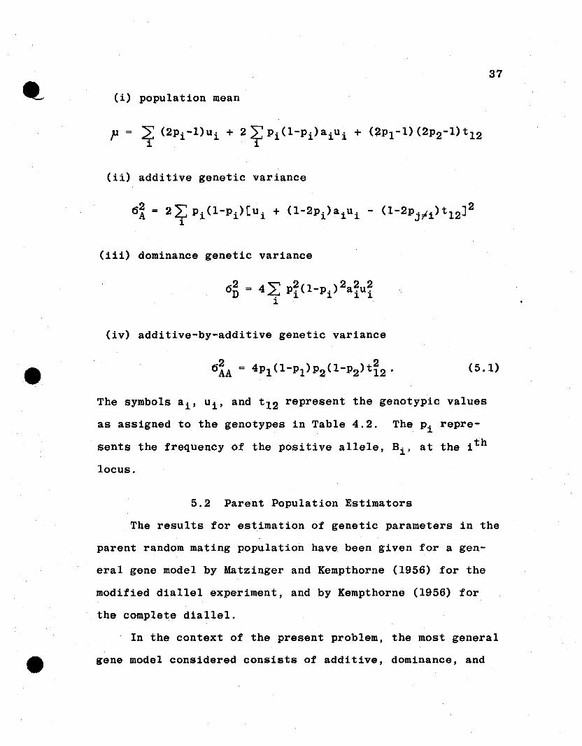
(i) population mean
p = 4 (2Pi-1)Ui + 24: Pi(1-Pi)aiu i + ( 2P1-1) (2P2-1)t121 1
(ii) additive genetic variance
(iii) dominance genetic variance
(iv) additive-by-additive genetic variance
(5.1)
The symbols ai' ui' and t12 represent the genotypic values
as assigned to the genotypes in Table 4.2. The Pi repre
sents the frequency of the positive allele, Bi , at the i th
locus.
5.2 Parent Population Estimators
The results for estimation of genetic parameters in the
parent random mating population have been given for a gen-
era1.gene model by Matzinger and Kempthorne (1956) for the
modified dia11e1 experiment, and by Kempthorne (1956) for
the complete dia11e1.
In the context of the present problem, the most general
gene model considered consists of additive, dominance, and
38
additive-by-additive epistasis at two loci,each with two
alleles. The mean and genetic variances of the parent popu
lation are those shown in (5.1) with the gene frequencies
shown in (5.1); i.~., the frequency of the positive allele,
Bi , at the i th locus is Pi.
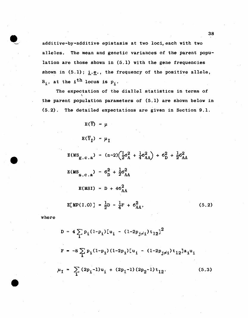
The expectation of the diallel statistics in terms of\
the parent population parameters of (5.1) are shown below in
(5.2). The detailed expectations are given in Section 9.1.
E(y) = )J
E(MS )s.c.a
E(MSI)
(5.2)
where
(5.3)
(5.4)
39
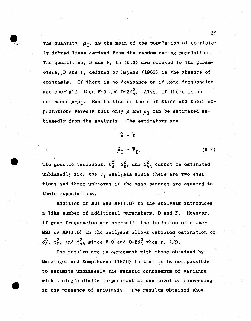
The quantity, PI' is the mean of the population of complete
ly inbred lines derived from the random mating population.
The quantities, D and F, in (5.3) are related to the param
eters, ,D and F, defined by Hayman (1960) in the absence of
epistasis. If there is no dominance or if gene frequencies
are one-half, then F=O and D=26~. Also, if there is no
dominance P=PI' Examination of the statistics and their ex
pectations reveals that only p and PI can be estimated un
biasedly from the analysis. The estimators are
A -]J == Y
1\ -PI == YI •
222The genetic variances, 6A, 6D, and 6AA cannot be estimated
unbiasedly from the Fl analysis ~inc~ there are two equa
tions and three unknowns if the mean squares are equated to
their expectations.
Addition of MSI and MP(I.O) to the analysis introduces
a like numbe~ o,f additional parameters, D and F. However,
if gene frequencies are one-half, the inclusion of either
MSI or MP(I.O) in the analysis allows unbiased estimation of. \
222 26A, 0D' and·6.AA since F=O and D=26A when Pi=1!2.
The results are in agreement with those obtained by
Matzinger and Kempthorne (1956) in that it is not possible
to estimate unbiasedly the genetic components of variance
with a single diallel experiment at one level of inbreeding
in the presence of epistasis. The results obtained show
40
that the present gene model is sufficient to indicate that
inclusion of more epistatic effects in the model only in
creases the difficulties of estimation from the dia11e1
analysis.
In the absence of epistasis, there is a change of defi
nition for the genetic parameters in (5.1) associated with
the reference population and a change in the expected values
of the statistics associated with the dial1e1 analysis. The
population parameters in the absence of epistasis are ob
tained from (5.1) by allowing t 12=0 and extending the model·
to include m loci. The expectations of the dia11e1 stat is-
tics are obtained in the manner described earlier and demon-
strated for the more complete genetic model in Section 9.1.
The resulting expectations are those given in (5.2) with the
a~A terms omitted.
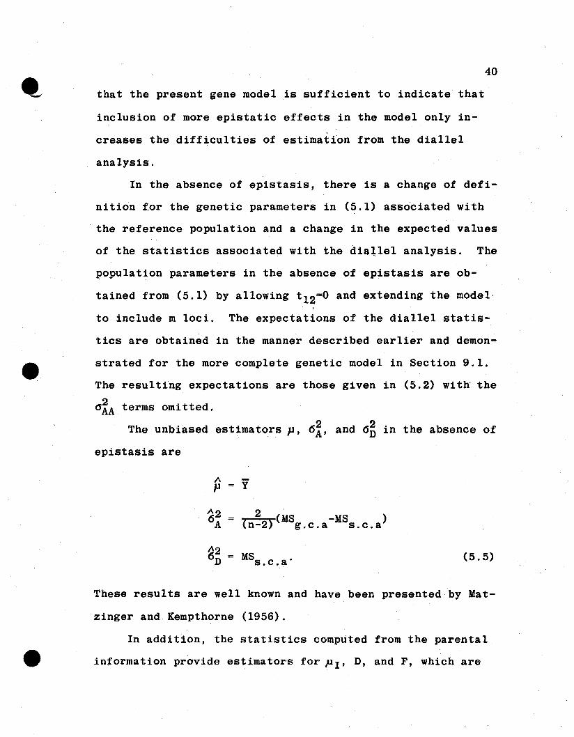
The unbiased estimators p, 6~, and 6~ in the absence of
epistasis are
1\P = Y
2(MS -MS )(n-2) g.c.a s.c. a
(5.5)
These results are well known and have been presented by Mat-
zinger and Kempthorne (1956).
In addition, the statistics computed from the parental
information provide estimators for PI' D, and F, which are
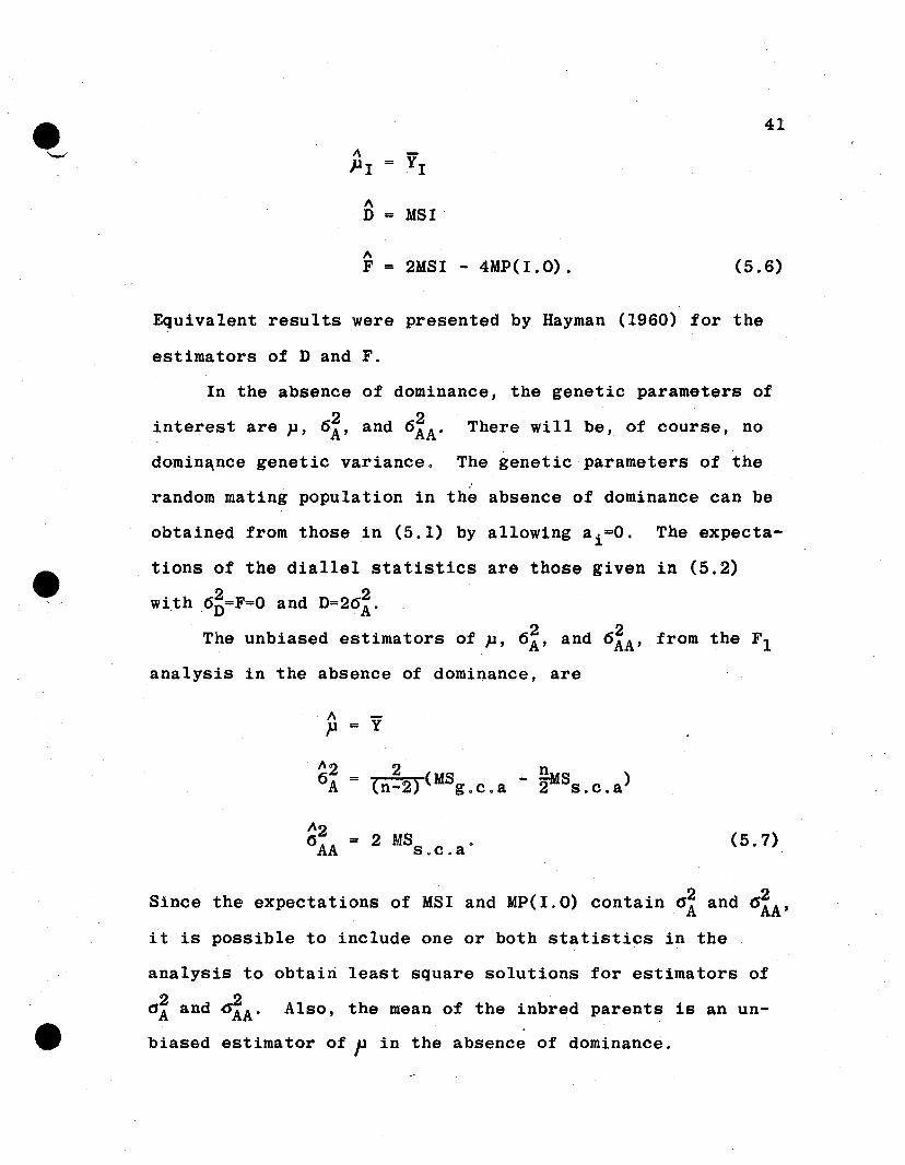
Equivalent results were presented by Hayman (1960) for the
estimators of D and F.
In the absence of dominance, the genetic parameters of
interest are p, 6~, and 6~A' There will be, of course, no
domin~nce genetic variance. The genetic parameters of the
random mating population in the absence of dominance can be
obtained from those in (5.1) by allowing ai=O. The expecta
tions of the dia1le1 statistics are those given in (5.2)2 2with 6D=F=0 and D=26A.
2 2The unbiased estimators of p, 6A, and 6AA , from the Fl
analysis in the absence of dominance, are
p = y
A20AA = 2 MSs.c.a (5.7)
Since the expectations of MSI and MP(I.O) contain a~ and 6~A'
it is possible to include one or both statistics in the
analysis to obtain least square solutions for estimators of
o~ and 6~A' Also, the mean of the inbred parents is an un
biased estimator of f in the absence of dominance.

•-- 42
5.3 Derived Population Estimato~s
5.3.1 General Remarks. In this section, the dia11e1
estimators are obtained for genetic parameters of the random
mating population derived entirely from the completely in-
bred parents of the dial1e1 cross, referred to as the de~
rived population. The gene frequencies of the derived popu-
lation are identical with the gene frequencies of the set of
inbred lines from which the population was derived in the
absence of forces that change gene frequency.
Ordinarily, the estimators for the derived population
parameters are obtained by equating the dial1e1 statistics
to their expectations in terms of the derived population ge-
netic parameters. Then solutions for the genetic parameters
in terms of the diallel statistics are taken as the estima-
tors. However, only the conditional expectations of the
diallel statistics are used, since we are concerned only
with those samples that give rise to the same derived popu~
lation. Such estimators are considered to be conditionally
unbiased.
However, the average values of the derived population
paramet~rs can be expressed as linear functions of the par
ent population parameters," Since the expectations of the
statistics are known in terms of the parent population pa-
rameters, it is most convenient to make use of the linear
relationships of the two sets of parameters in solving for
unbiased estimators of the derived population parameters.
43
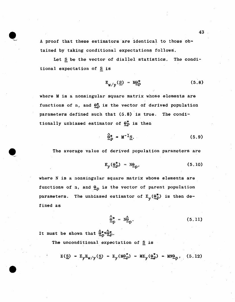
A proof that these estimators are identical to those ob-
tained by taking conditional expectations follows.
Let S be the vector of diallel statistics. The condi-
tional expectation of S is
(5.8)
where M is a nonsingular square matrix whose elements are
functions of n, and 9p is the vector of derived population
parameters defined such that (5.8) is true. The condi
tionally unbiased estimator of ~ is then
(5.9)
The average value of derived population parameters are
(5.10)
where N is a nonsingular square matrix whose elements are
functions of n, and ~p is the vector of parent population
parameters. The unbiased estimator of Ey(9~) is then de
fined as
(5.11)
It must be shown that ~~$~.
The unconditional expectation of S is
E(S)
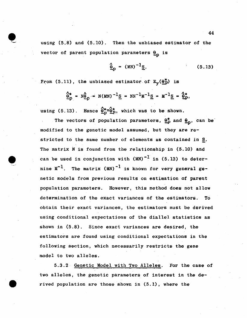
44
using (5.8) and (5.10). Then the unbiased estimator of the
vector of parent population parameters ~ is
(5.13)
,F~om (5.11), the unbiased estimator of' Ey(~) is
using (5.13).1'\ 1\
Hence 9*~9* which was to be shown.-p ~"
The vectors of population parameters, ~p and !p' can be'
modified to the genetic model assumed, but they are re-
stricted to the same number of elements as contained in S.-The matrix N is found from the relationship in (5.10) and
can be used in conjunction with (MN)-l in (5.13) to deter
mine M- l . The matrix (MN)-l is known for very general ge-
netic models from previous results on estimation of parent
population parameters. However, this method does not allow
determination of the exact variances of the estimators. To
obtain their exact variances, the estimators must be derived
using conditional expectations of the diallel statistics as
shown in (5.8). Since exact variances are desired, the
estimators are found using conditional expectations in the
following section, which necessarily restricts the gene
model to two alleles.
5.3.2 Genetic Model with Two Alleles. For the case of
two alleles, the genetic parameters of interest in the de
rived population are those shown in (5.1), where the
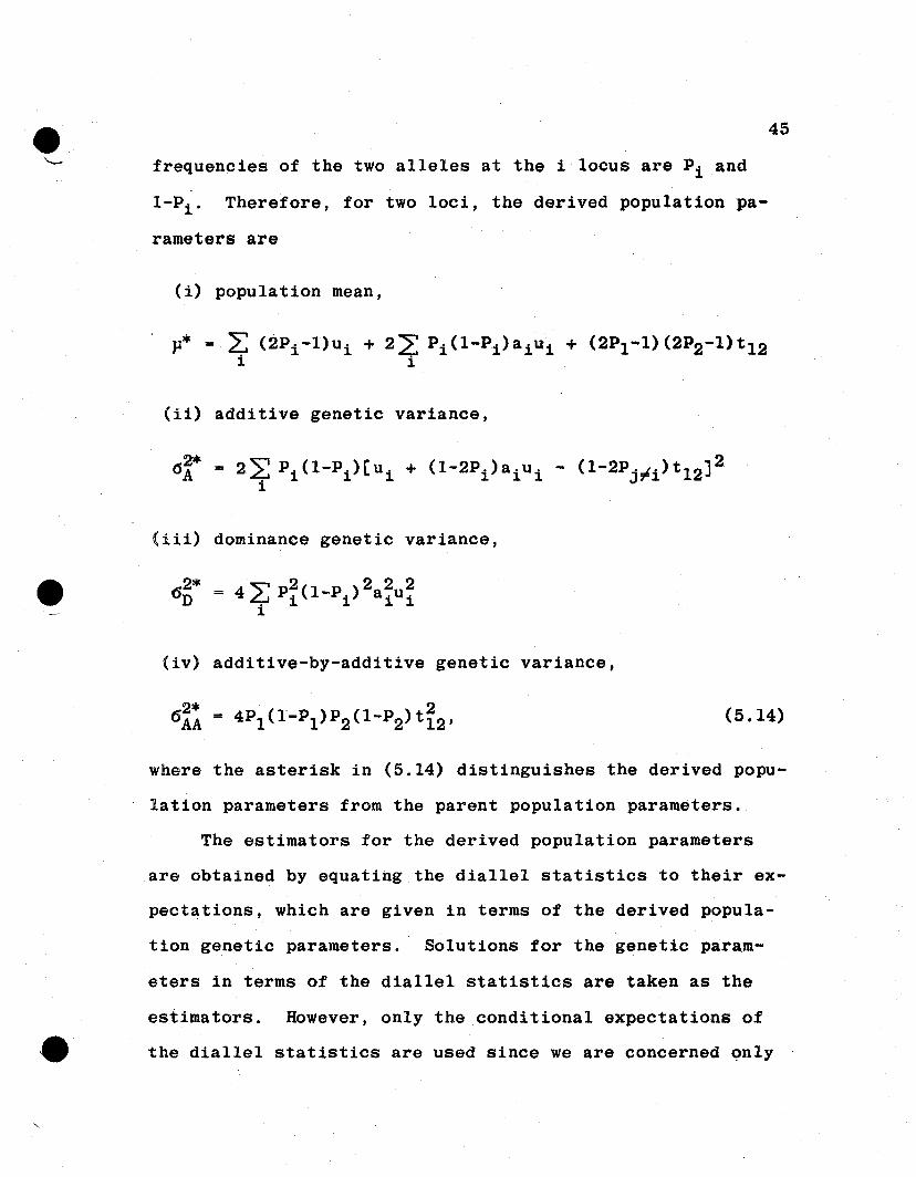
45
frequencies of the two alleles at the i locus are Pi and
I-Pi. Therefore, for two loci, the derived population pa
rameters are
(i) population mean,
(ii) additive genetic variance,
(iii) dominance genetic variance,
(iv) additive-by-additive genetic variance,
(5.14)
where the asterisk in (5.14) distinguishes the derived popu-
lation parameters from the parent population parameters.
The estimators for the derived population parameters
are obtained by equating the diallel statistics to their ex-
pectations, which are given in terms of the derived popula-
tion genetic parameters. Solutions for the genetic param-
eters in terms of the diallel statistics are taken as the
estimators. However, only the conditional expectations of
,~ the dial leI statistics are used since we are concerned only
46
with those samples that give rise to the same derived popu-
lation.
The conditional expectations for the diallel statistics
of Section 4.2 are shown in Section 9.1. The conditional
expectation of the mean of the Fl's is
(5.15)
where p~=~ (2Pi-l)ui+(2Pl-l) (2P2-l)t12 is the mean of thel.
population of completely inbred lines obtained from the de-
rived population. The coefficient of p* illustrates an in
crease in the amount of heterozygosis in the derived popula-
tion relative to that of the parent population.
The conditional expectation of the mean of the diallel
parents is
(5.16)
The conditional expectations of the mean squares and
product of the diallel analysis are
47
n *'- (n-2) n
n 2
+ 2(n-l) (n-2)F*
+ n n*' _ n iF*(n-2) (n-3) (n-2) (n-3)
EW/y[MP(I.O)]
= n D* 4n(n-2)~*(n-l) + (n-l)2 AA
n n* n(n-4) 6¥* n2 iF*2 (n-l) + (n-l) 2 AA - 4(n-l) (n-2) (5.17)
2* 2* 2* ( 14)The parameters, 6A ' 6n ' and 6AA , are shown in 5. .
and F* are the derived population equivalents ton and F
n*
shown in (5.3).
Solving (5.15) and (5.16) for p~ and p*, the following
unbiased estimators are obtained
A* = (n-l)y + lYI'P n n (5.18)
,Observation of equations (5.17) reveals that there are
four equations in five unknowns, which precludes obtaining
unbiased estimators of any of the genetic components of
variance except with gene frequencies of one-half. In that
•
48
case, F*=O and D*=2~*, and inclusion of either MSI or
MP(I.O) allows unbiased estimation of the genetic components
of variance--a situation analogous to that encountered for
estimation of components of genetic variance in the parent
population.
The additive and dominance gene model in the absence of
epistasis is considered by allowing t12=O in all formulas
and extending to m loci. In the absence of epistasis, the
conditional expectations of the diallel statistics are those
shown in (5.15) through (5.17) with the 6~~ terms omitted.
Setting the statistics equal to their conditional ex-
pectations and solving for the parameters gives the follow-
ing set of estimators for the derived population parameters.
~D2* = (n-l)(n-3)MS + 4(n-1)2MSn(n-2) s.c.a n3 (n-2) g.c.a
(n-l)- In Y + -yn I
= (n-l)en
(n-1) (n-2)/\2 F.
n(5.19)
49
It is important to realize that the unbiased estimators
for derived population parameters are unbiased over those
diallel samples that lead to the same derived population,<
i.~., those dial leI samples having the same set of Pi' which
is quite different from obtaining unbiased estimators from a
fixed sample for its specific derived population.
If for the additive and dominance model the parental
* 2*analysis is ignored, one set of estimators for p , 6A ' and
2*6 n obtained from the analysis of the FIls is
( ~2*) 2(n-l) (n-2)MSvA b~= n3 g.c.a
(dn2*)b = (n-I)(n-2)(n-3)MS3 s.c.a·
n(5.20)
However, there is a bias associated with each of the estima-
tors in (5.20). The average bias for each of the estimators
is
4(n-l) 2 "C"l 2 2= - 3 ~ P.(l-Pi)a.u ... 1 1 1n 1
(5.21)
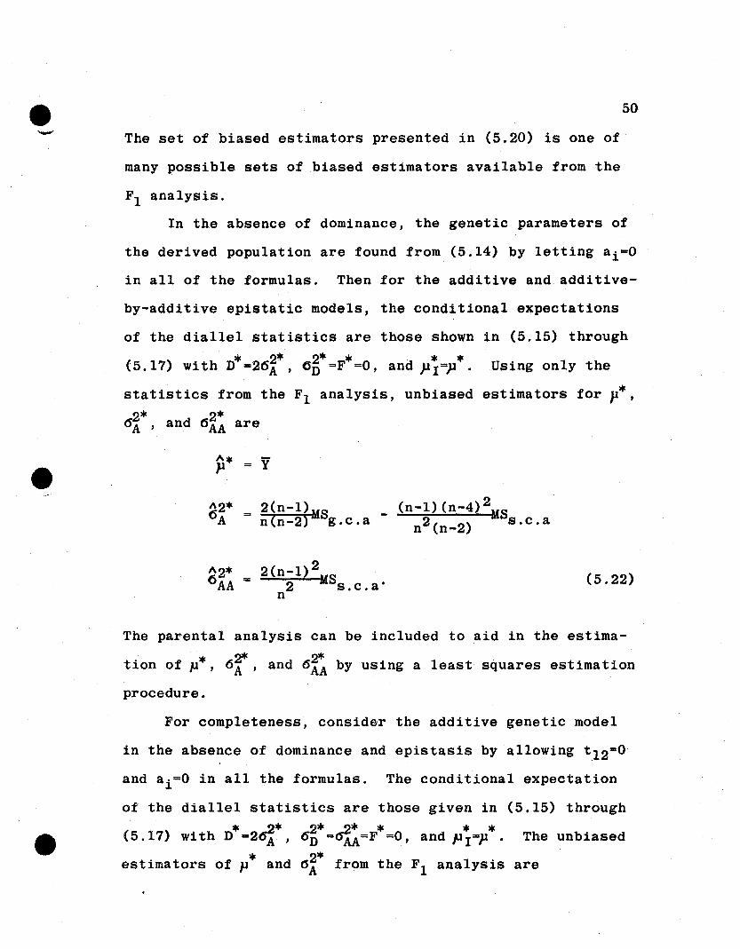
--50
The set of biased estimators presented in (5.20) is one of
many possible sets of biased estimators available from the
Fl analysis.
In the absence of dominance, the genetic parameters of
the derived population are found from (5.14) by letting ai=O
in all of the formulas. Then for the additive and additive-
by-additive epistatic models, the conditional expectations
of the diallel statistics are those shown in (5.15) through
* 2* 2* * * *(5.17) with D =26A ' 6D =F =0, and PI=P. Using only the
statistics from the Fl analysis, unbiased estimators for p*,2* 2*6A ' and (5AA are
A* }1 = Y
2(n-l)2MS2 s.c.a·
n(5.22)
The parental analysis can be included to aid in the estima-
* 2* 2*tion of p , 6A ' and 6AA by using a least squares estimation
procedure.
For completeness, consider the additive genetic model
in the absence of dominance and epistasis by allowing t12=0
and ai=O in all the formulas. The conditional expectation
of the diallel statistics are those given in (5.15) through
* _2* 2* _2* * * *(5.17) with D =26A ' 6D =O-AA=F =0, and Pr=P. The unbiased
* 2*estimators of p and 6A from the FI analysis are
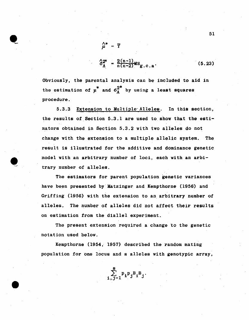
51
. (5.23)
5.3.3 Extension to Mu1tip1eoA11eies. In this section,
the results of Section 5.3.1 are used to show that the esti-
mators obtained in Section 5.3.2 with two alleles do not
change with the extension to a multiple allelic system. The
result is illustrated for the additive and dominance genetic
model with an arbitrary number of loci, each with an arbi-
trary number of alleles.
The estimators for parent population genetic variances
have been presented by Matzinger and Kempthorne (1956) and
Griffing (1956) with the extension to an arbitrary number of
alleles. The number of alleles did not affect their results
on estimation from the diallel experiment.
The present extension required a change to the genetic
notation used below.
Kempthorne (1954, 1957) described the random mating
population for one locus and s alleles with genotypic array,
sL p.p.B.B ..
i, j=l ~ J ~ J
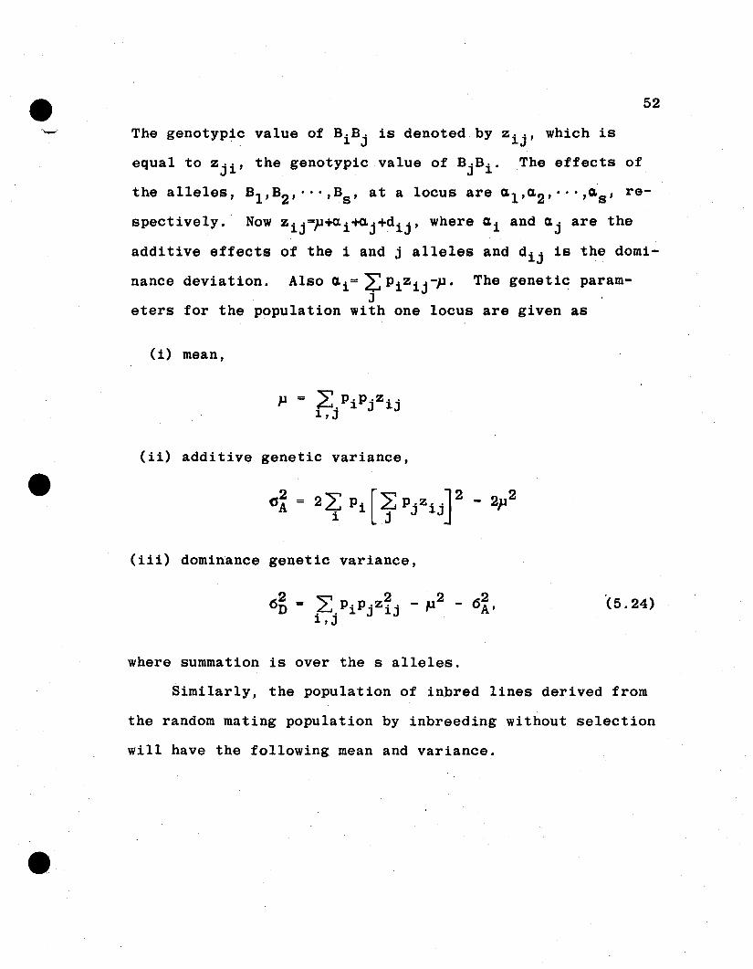
52
The genotypic value of BiBj is denoted by Zij' which is
equal to Zji' the genotypic value of BjBi . The effects of
the alleles, B1 ,B2 , ··.,Bs ' at a locus are u 1 ,U2 '···'Us ' re
spectively. Now Zij=P+«i+«j+dij , where Ui andUj are the
additive effects of the i and j alleles and dij is the domi
nance deviation. Also u i =~ PiZij-P. The genetic param-J
eters for the population with one locus are given as
(i) mean,
(ii) additive genetic variance,
(iii) dominance genetic variance,
62 = L p. p .z~. - p2D i,j 1 J 1J .
where summation is over the s alleles.
"(5.24)
Similarly, the population of inbred lines derived from
the random mating population by inbreeding without selection
will have the following mean and variance.
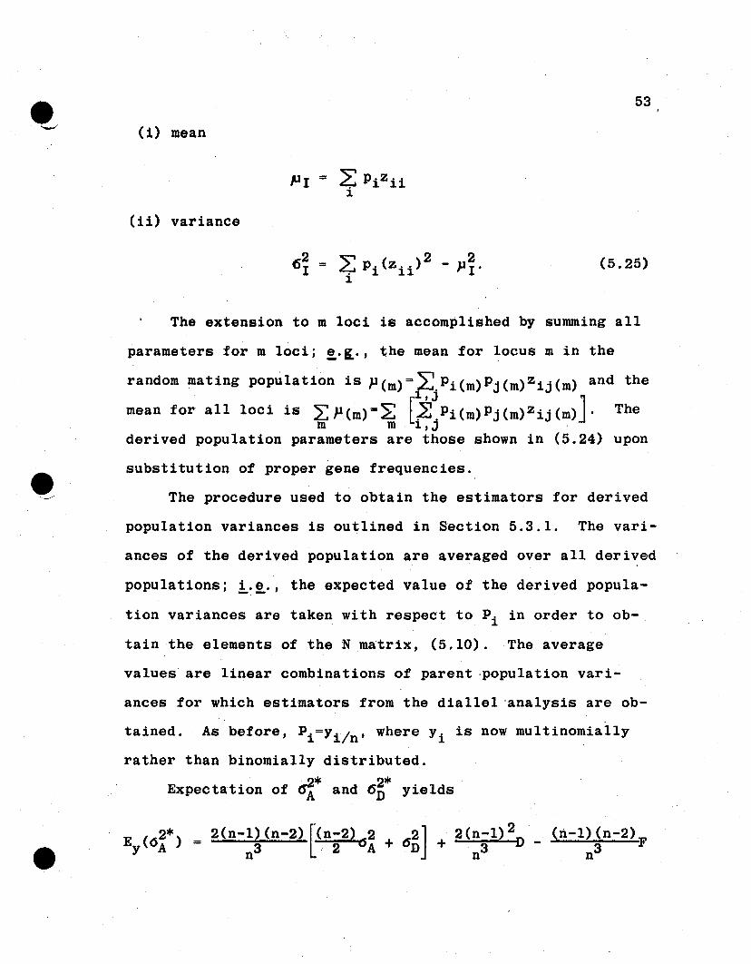
53
(i) mean
(ii) variance
(5.25)
The extension to m loci is accomplished by summing all
parameters for m loci; ~.~., the mean for locus m in the
random mating population is P(m)=L:,Pi(m)PJ'(m)Zij(m) and the. 1. , J
mean for all loci is LP(m)=~ L~Pi(m)Pj(m)Zij(m)J. Them m 1.,j .
derived population parameters are those shown in (5.24) upon
substitution of proper gene frequencies.
The procedure used to obtain the estimators for derived
population variances is outlined in Section 5.3.1. The vari
ances of the derived population are averaged over all derived
populations; !..2,.., the expected value of the derived popula-
tion variances are taken with respect to Pi in order to ob
tain the elements of the N matrix, (5.10). The average
values are linear combinations of parent -population vari-
ances for which estimators from the diallel "analysis are ob
tained. As before, Pi=Yiln' where Yi is now multinomially
rather than binomially distributed.:..2* 2*Expectation of OA and 60 yields
E (62*) - 2(n-l) (n-2) [(n-2) 62 602] + 2 (:;1) 2D"_ (Ii-I) (n-2) FY A - n3 "2 A + n3
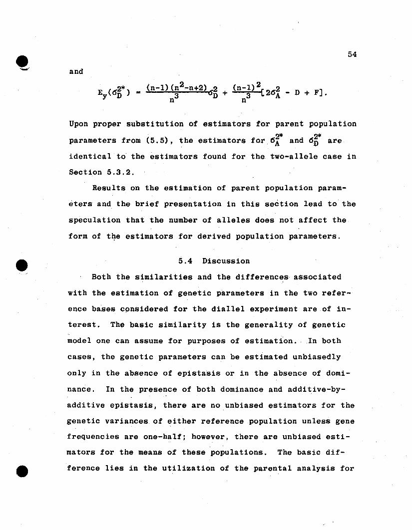
54
and
Upon proper substitution of estimators for parent population
parameters from (5.5), the estimators for.6~ and 6~* are
identical to the estimators found for the two-allele case in
Section 5.3.2.
Results on the estimation of parent population param
eters and the brief presentation in this section lead to the
speculation that the number of alleles does not affect the
form of t~e estimators for derived population parameters.
5.4 Discussion
Both the similarities and the differences associated
with the estimation of genetic parameters in the two refer-
ence bases cpnsidered for the dial leI experiment are of in-
terest. The basic similarity is the generality of genetic
model one can assume for purposes of estimation. In both
cases, the genetic parameters can be estimated unbiasedly
only in the absence of epistasis or in the absence of domi-
nance. In the presence of both dominance and additive-by
additive epistasis, there are no unbiased estimators for the
genetic variances of either reference population unless gene
frequencies are one-half; however, there are unbiased esti-
mators for the means of these populations. The basic dif-
ference lies in the utilization of the parental analysis for
55
estimation. In the presence of dominance, statistics from
the parental analysis are required for unbiased estimators
of genetic parameters of the derived population, whereas
they are not required for the parent population estimators.
The results of Section 5.3.1 provide a convenient means
for obtaining unbiased estimators of the derived population
parameters for a general gene model. The method should prove
useful in extending results to mating designs other than the
diallel in that one can dispense with the formulation of the
statistics of the analysis in terms of the sampling variables
and genotypic values as was done in Section 4. It is only
necessary to obtain the average value of the derived popula-
tion parameters as a linear function of the parent population
parameters and take usual estimators from the analysis of
parent population parameters to obtain an unbiased. estimator
of the linear function.
56
6. VARIANCES OF ESTIMATORS
6.1 Introduction
The exact variances of the unbiased estimators for the
parent population and derived population parameters are ob
tained for the genetic model, including only additive and
dominance effects with two alleles at each locus. The vari-
ances of the biased estimators of derived population param-
eters (5.21) are also considered .
. The variances of the derived population estimators are
compared to the variances of the parent population esti-
mators as an indication of the relative efficiency of the
derived population estimators.
Initially, only variances of the genetic portion of the
estimators shown in (5.5) and. (5.l9) are presented. The
consequences of random experimental error and replication
are discussed in Section 6.5.
6.2 Exact Variances of Parent
Population Estimators
The estimators of parent population parameters in the
absence of epistasis are
1\ }J = Y"2 26A = (n_2){MSg .c . a - MSs . c . a )
"'26D = MSs . c . a '
as shown in (5.5).
57
The exact variance of ~~ is
4 2[V(MSg c a) + V(MS s c a)(n-2) . . . .
- 2 COV(MSg . c .a , MBs . c . a )],
and the exact variance of a~ is V(an2 )=V(MS ).s.c.a
V(MBg . c . a ), V(MBs . c .a ), and Cov(MSg . c . a , MBs,c.a) are
obtained by use of the mean squares shown in (4.14) with the
variables Pi and Wij' which are binomially and hypergeo
metrically distributed, respectively. The variances and co-
variance are found from the expectations,
V(MSg,c,a) = E{MSg . c . a )2 - [E(MBg . c ,a)]2
V(MBs,c.a) = E(MSs ,c.a)2 - [E(MSs ,c.a)]2
e and
Cov(MBg,c,a' MBs,cta) = E[(MSg.c,a)(MSs.c.a)]
- E(MSg.c.a)E(MBs.c.a)·
Due to their complexity, the derivations of the above
variances and covariance are given in Section 9.2. The
final form of the two variances and covariance are shown
in Table 6,1. At the present time, the formulas of Table
6.1 appear to be unfactorable in their present form. How-
ever, with the simplifying assumption of only additive gene
effects, the variance of MSg.c,a in Table 6.1 is a function
of the variance of the sampling variance of gene frequencies.
For example, in the absence of dominance, the variance of
the estimator for additive genetic variance for one locus
can b~ expressed as
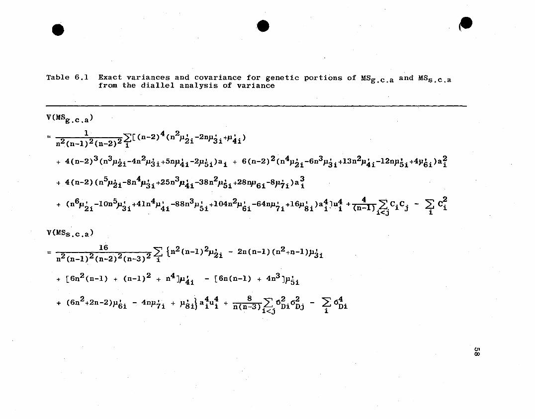
e e "Table 6.1 Exact variances and covariance for genetic portions of MSg . c . a and MSs . c . a
from the dia11e1 analysis of variance
V(MSg . C •a )
= 2 12 2~[(n-2)4(n2p2'·-2nP3'·+P4'·)n (n-1) (n-2) i 1 1 1
+ 4(n-2)3(n3p2i-4n2p3i+snp4i-2PSi)ai + 6(n-2)2(n4p2i-6n3P3i+13n2P4i-12nP5i+4P6i)a~
+ 4(n-2)(nSp2i-8n4p3i+2Sn3p4i-38n2p5i+28nP6i-8P7i)a~
+ ( n6P2'· -10nSp3' . +41n4P4' . -88n3Ps' . +104n2P6' . - 64nP7' . +16P8' . )a~Ju~ + ( :1) L: Ci CJ. - 2: C~1 1. 1 1 1 1 1 1 1 n i<j i
V(MSs •c •a )
= 16 ~ { 2 2n2 (n-1)2 (n-2)2(n-3)2 -? 1.n (n-1) Jl2i - 2n(n-1) (n
2+n-1)}13i
+ [6n2 (n-1) + (n-1)2 + n4Jp4i - [6n(n-1) + 4n3 JpSi
+ (6n2+2n-2)P6" - 4nP7'· + PS' .1 a~u~ + (~3) L 0n2 .6n2 . - 2: 6n
41·1 1 1) 1 1 n n " 1 J .. . 1<J . 1
C1l(Xl
e
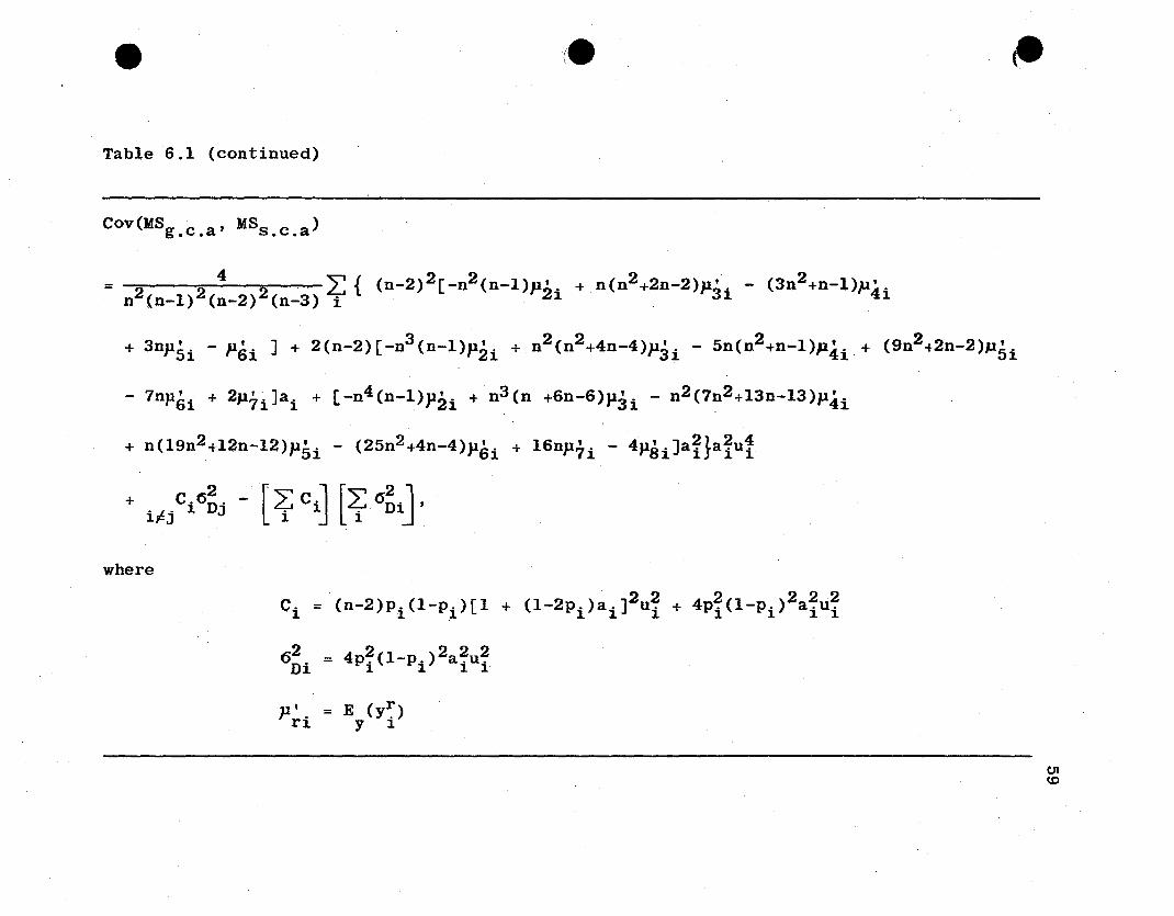
Table 6.1 (continued)
COV(MSg •c •a ' MSs • c •a )
ie ~
_ 4 ""'{ 2 2 2·- n2 (n-l)2(n-2)2(n-3) ~ (n-2) [-n (n-l)P2i + n(n +2n-2)P3i - (3n
2+n-l)P4i
+ 3nPSi - P6i J + 2(n-2)[-n3 (n-l)P2i + n2 (n2 +4n-4)P3i - 5n(n2+n-l)P4i + (9n2+2n-2)PSi
- 7nP6i + 2P7i]ai + [-n4 (n-l)P2i +n3 (n +6n-6)P3i - n2 (7n2 +13n-13)P4i
+ n(19n2 +12n-12)PSi - (25n2 +4n-4)P6i + 16nP7i - 4P8iJa~}a~u1
+ C.On2
. - [2: c.] [2: (52.J,iFj ~ J i ~ i n~
where
22222 2Ci = (n-2)Pi(1-Pi)[1 + (1-2Pi)a i ] u i + 4Pi (1-Pi) aiui
6 2Di
J1~i
= 4p~(1-p.)2a~u~~ ~ ~ ~
= E (y~)Y ~
01CD
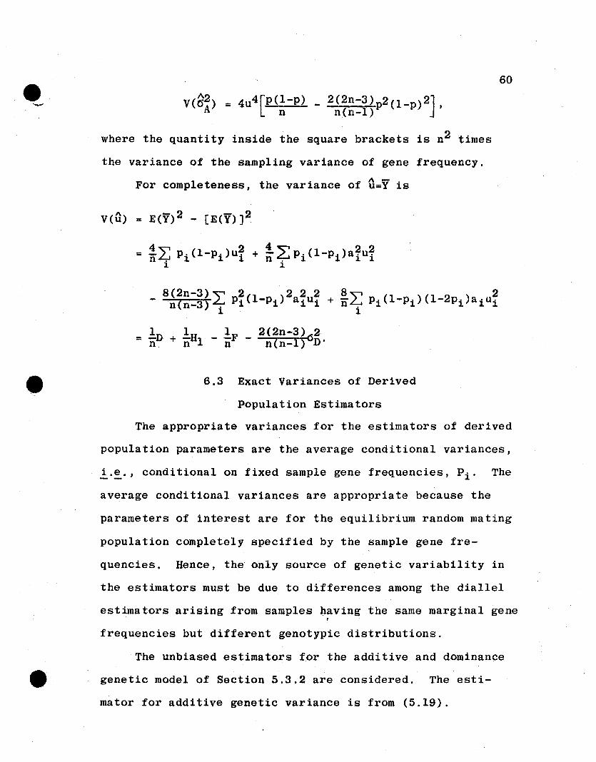
-60
where the quantity inside the square brackets is n2 times
the variance of the sampling variance of gene frequency.
For completeness, the variance of Q=y is
8(2n-3)~ P~(1-p.)2a~u~ + 8n~, Pl' (1-Pi)(1-2Pl·)al,u2l'n(n-3)~ 1 1 1 1 ~
1 1
= 10 + nlHl - !F _ 2(2n-3)62n n n(n-l) D'
6.3 Exact Variances of Derived
Population Estimators
The appropriate variances for the estimators of derived
population parameters are the average conditional variances,
i.~., conditional on fixed sample gene frequencies, Pi' The
average conditional variances are appropriate because the
parameters of interest are for the equilibrium random mating
population completely specified by the sample gene fre-
quencies. Hence, the· only source of genetic variability in
the estimators must be due to differences among the diallel
estimators arising from samples having the same marginal gene. .
frequencies but different genotypic distributions.
The unbiased estimators for the additive and dominance
genetic model of Section 5.3.2 are considered. The esti-
mator for additive genetic variance is from (5.19).
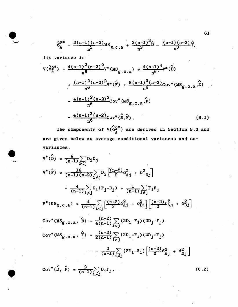
61
~2* = 2(n-l)(n-2)MS + 2(n-l)2£ (n-l)(n-2)AA n3 g. c •a n3 - n3 F.
Its variance is
- 4(n-l):(n-2)coV*(D,9). (6.1)n
"'2*The components of V(6A
) are derived in Section 9.3 and
are giv~n below as average conditional variances and co
variances.
.'-......-, '"V*(D)
V*(F)
= 4 "" DiD.(n-l) .L..... Jl.<J
= 16 2:: D. [(n-2) 62(n-l)(n-2)i~j l. [2 Aj
+ 4 ~D.(F.-D.) + 1 LF.F.(n-l) i~j l. J J (n-l) i~j l. J
V*(MS ) = 4 ~[(n-2)62. + 62 .J" f(n-2)62 .g.c.a (n-l)i~· 2 Al. D~ L 2 AJ
1\COV*(MSg •c . a , D)
"-Cov*(MSg . c .a ' F)
(6.2)
62
where
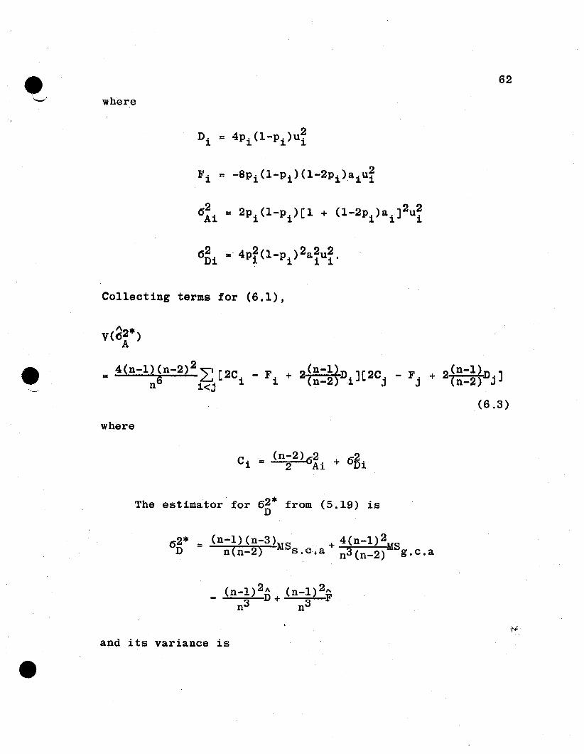
Collecting terms for (6.1),
V(~2·)A
- 4(n-l) (n_2)2" [2C F 2~n-l~D ][2C F 2(n-l)D J- n6 «j i - i + n-2 i j - j + (n-2) j
(6.3)
where
The estimator for 6~* from (5.19) is
and its variance is
63
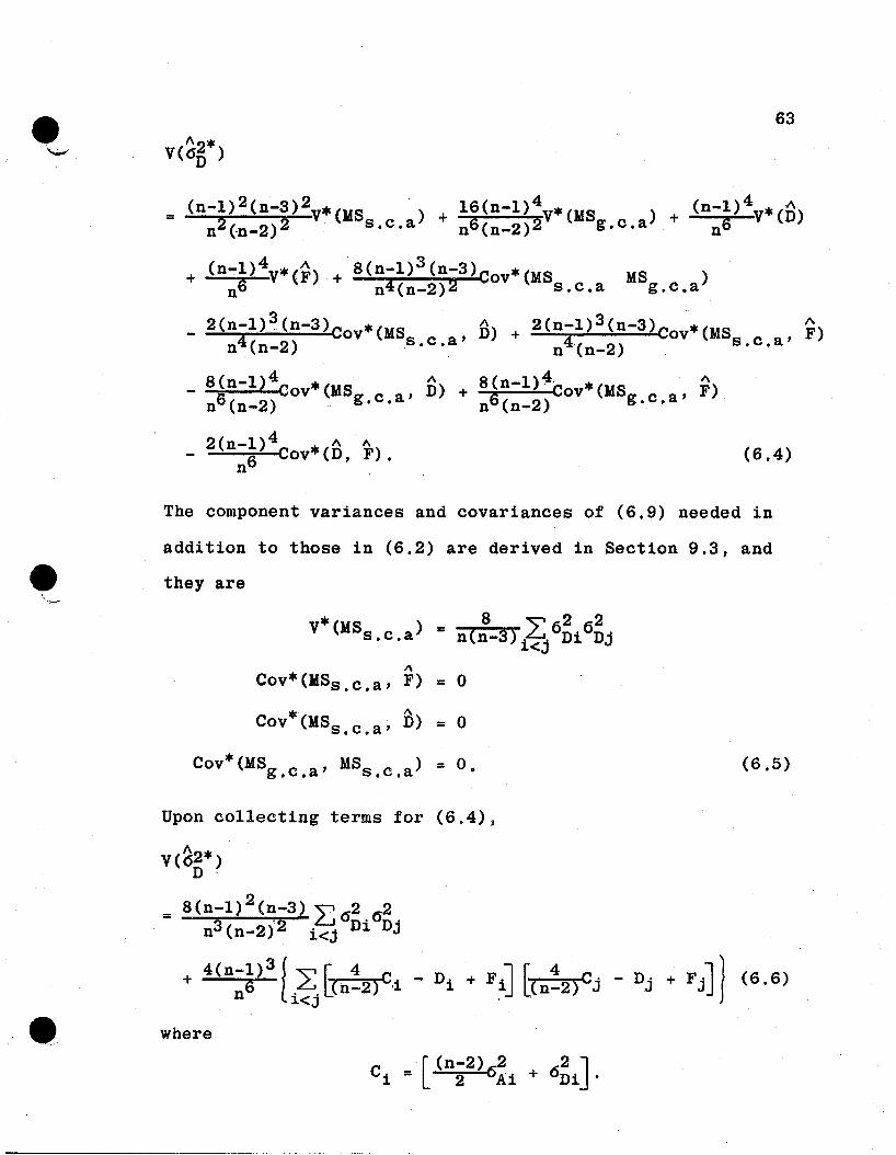
V(~2*)D
2 2 . 4 ( )4= (n-1) (n-3) ¥*(MS ) + 16(n-1) ¥*(MS ) + n-~ v*(n)n2(-n_2)2 s.c.a n6(n_2)2 g.c.a n
4 . 3+ (n-1) ¥*(;) + 8(n-l) (n-3)CoV*(MS MS
g.c
.a
)n6 n4(n-2)2 s.c.a
2(n-1)3(n-3)C *(MS fi) + 2(n-1)3(n-3)CoV*(MS , F)n4(n-2) ov s.c.a' n'(n-2) s.e.a
8(n-1)4 * A 8(n-1)~c'ov*(MS , F~)6 COY (MSg c a' D) + 6 g c an (n-2) . . n (n-2) . .
2(n-~)4cov*(a, F). (6.4)n
The component variances and covariances of (6.9) needed in
addition to those in (6.2) are derived in Section 9.3, and
they are
V*(MS ) = 8." 62 .62s.c.a ( 3) LJ D Djn n- i<j 1
1\
Cov*(MSs . c . a , F) = 0
COV*(MSs . c . a ' a) = 0
CoV*(MSg . c . a ' MSs . c . a ) = O.
Upon collecting terms for (6.4),
(6.5)
V(~2*)D'
= 8(n-1) 2 (n-3) :6 62 62n3 (n-2)2 i<j Di Dj
+ 4(n-~)3! L [<n:2)C'i ~ Di + F,i] [cn:2)Cj - Dj + FjJ 1 (6.6)n ~i<j .
where
[(n-2) 2 2 ]Ci = 2 6Ai + 6Di .
64
The conditional variance of the estimator of p*,
(5.19), is zero; hence, the average conditional variance
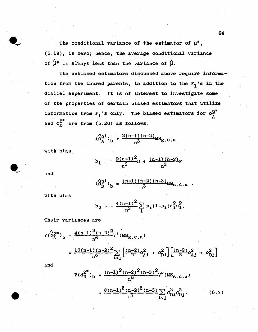
of ~* is always less than the variance of p.The unbiased estimators discussed above require informa-
tion from the inbred parents, in addition to the Fl's in the
diallel experiment. It is of interest to investigate some
of the properties of certain biased estimators that utilize
information from Fl's only. O· 2*The biased estimators forA
and 6~* are from (5.20) as follows.
2(n-l) (n-2)1I83 . g.c.a
n
with bias,
and
= (n-l)(n-2)(n-3)MS3 s.c.a '
n
with bias
Their variances are
1\V«(52*)A b
2 2= 4(n-l) (n-2) ¥*(MS )n6 g.c.a
and222= (n-l) (n-2) (n-3) ¥*(M8 . )
n6 s.c.a
8 (n-l)2 (n-2)2 (n-3) L: (j2 62= n7 . . Di Dj'
l.<J(6.7)
65
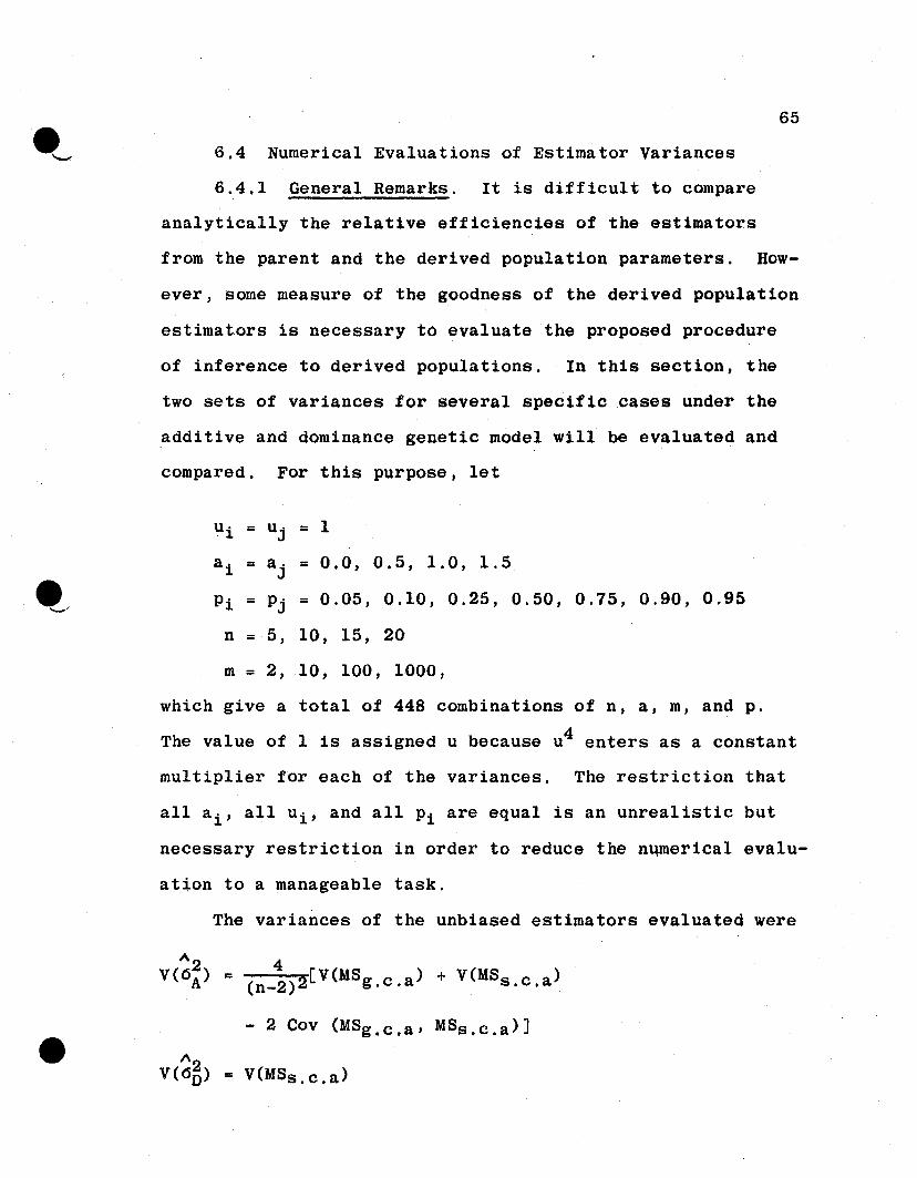
6.4 Numerical Evaluations of Estimator Variances
6.4.1 General Remarks. It is difficult to compare
analytically the relative efficiencies of the estimators
from the parent and the derived population parameters. How-
ever, some measure of the goodness of the derived population
estimators is necessary to evaluate the proposed procedure
of inference to derived populations. In this section, the
two sets of variances for several spe6ificcases under the
additive and dominance genetic model will be evaluated and
compared. For this purpose, let
u· = Uj = 1·1
a i = a j = 0.0, 0.5, 1.0, 1.5
Pi :::: Pj = 0.05, 0.10, 0.25, 0.50, 0.75, 0.90, 0.95
n :::: 5, 10, 15, 20
m = 2, 10, 100, 1000,
which give a total of 448 combinations of n, a, m, and p.
The value of 1 is assigned u because u4 enters as a constant
multiplier for each of the variances. The restriction that
all ai' all ui' and all Pi are equal is an unrealistic but
necessary restriction in order to reduce the n~merical evalu-
atton to a manageable task.
The variances of the unbiased estimators evaluated were
A 4V(6~) :::: (n_2)2[V(MSg .c . a ) + V(MSs . c .a )
- 2 Cov (MSg . c . a , MSs . c. a) ]
A
V(6~) = V(MSs . c . a )
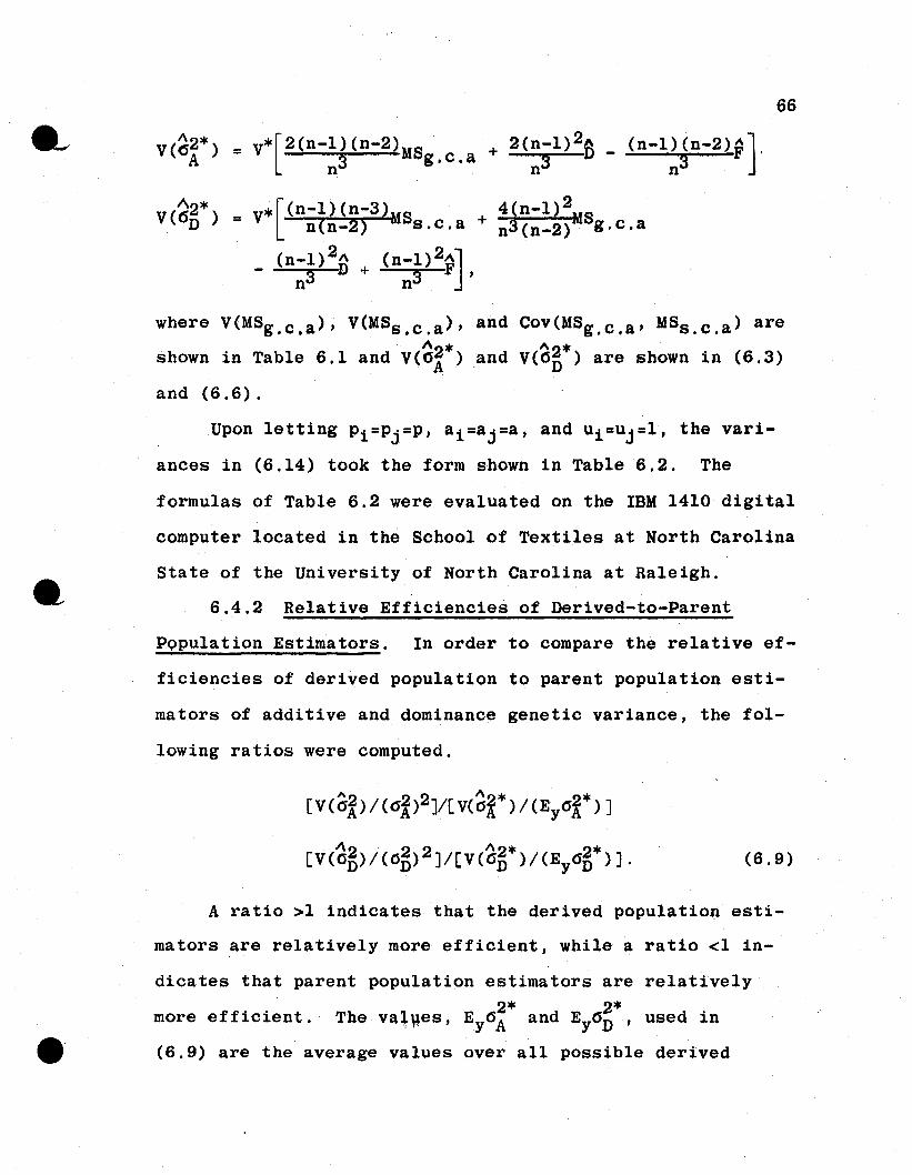
V(~~*) = v*[2(n-l)(n-2)MS + 2(n-l)28 _ (n-l)(n-2)F]'n3 g.e.a n3 n3
66
= v*[(n-l)(n-3)MS . +n(n-2) s.e.a
(n_l)2A (n-l)20 ]- 3 D+ 3 F,n n
4(n-l)2MSn3 (n-2). g.e.a
where V(MSg . e •a ), V(MSs . e . a )' and COV(MSg . e .a , MSs . c .a ) are
"2* "2*shown in Table 6.1 and V(OA ) and V(On ) are shown in (6.3)
and (6.6).
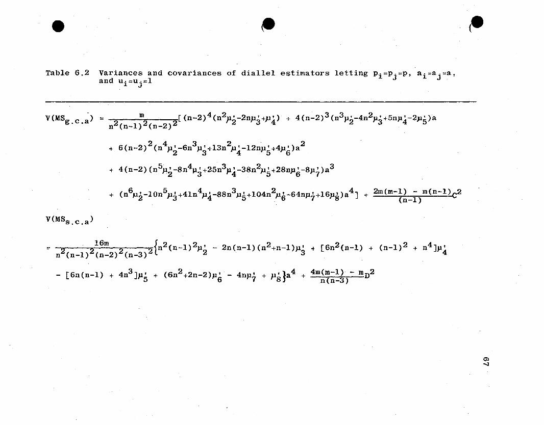
Upon letting Pi=Pj=P, ai=aj=a, and ui=Uj=l, the vari
ances in (6.14) took the form shown in Table 6.2. The
formulas of Table 6.2 were evaluated on the IBM 1410 digital
computer located in the School of Textiles at North Carolina
State of the University of North Carolina at Raleigh.
6.4.2 Relative Efficiencies of Derived-to-Parent
P9Pulation Estimators. In order to compare the relative ef-
ficiencies of derived population to parent population esti-
mators of additive and dominance genetic variance, the fol-
lowing ratios were computed.
[V(6~)/(6*)2]/[V(d~*)/(Ey6**)j
[V(~~)/(6~)2J/[V(6~*)/(Ey6~*)J. (6.9)
A ratio >1 indicates that the derived population esti-
mators are relatively more efficient, while a ratio <1 in-
dicates that parent population estimators are relatively
2* 2*more efficient. The v~l~es, Ey6A and Ey6D ' used in
(6.9) are the average values over all possible derived
e • ~
Table 6.2 Variances and covariances of dial1el estimators letting Pi=Pj=P, ai=aj=a,and ui:::Uj=1
V(MS -) = m. [(n-2)4(n2p'-2np'+p') + 4(n-2)3(n3p'-4n2p'+5np'-2p')ag.c.a n2 (n-1)2(n-2)2 2 3 4 2 3 4 5
2432" 2+ 6(n-2) (n Pi-6n P3+13n P4-12nPS+4P6)a
+ 4(n-2) (n5p'-8n4p'+25n3p'-38n2p'+28np'-8p')a32 3 4 567
+ (n6P2-10n5p3+41n4p4-88n3~5+104n2p6-64nP7+16P8)a4J + 2m(m-~) ~.m(n-1)C2
V(MSs . c • a )
~ 2 "216m
2 2{n2 (n-l)2Pi - 2n(n-1)(n2+n-l)p~ + [6n2 (n-l) + (n-l)2 + n4]p~n (n-l) (n-2) (n-3)
- [6n(n-l) + 4n3 Jp' + (6n2 +2n-2)p' - 4np' + p'la4 + 4m(m-l) - ID n25 6 7 8) n(n-3)
m~
e
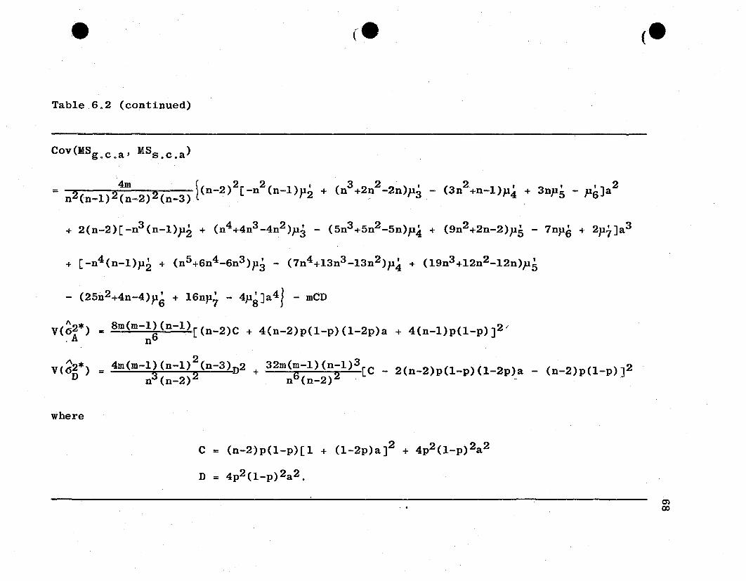
Table 6.2 (continued)
Cov(MSg . c . a ' MSs . c . a )
(e .(e
= 224m
2 f(n-2)2[-n2
(n-l)P2 + (n3
+2n2
-2n)P3 - (3n2
+n-l)P4 + 3nP5 - P6 Ja2n (n-I) (n-2) (n-3) l .
+ 2(n-2)[-n3 (n-l)P2 + (n4 +4n3 -4n2 )pj - (5n3 +5n2 -5n)P4 + (9n2+2n-2)PS - 7np6 + 2p7Ja3
+ [-n4 (n-l)P2 + (n5+6n4-6n3 )p3 - (7n4+l3n3 -l3n2 )p4 + (l9n3 +l2n2-l2n)P5
- (25n2+4n-4)p~ + l6np~ - 4p~Ja4} - mCD
"V(~~*) = 8m(m-l~(n-l)[(n_2)C + 4(n-2)p(l-p) (1-2p)a + 4(n-l)p(1-p)]2'n
V<62*) - 4m(m-l) (n-l)2(n-3)D2 + 32m(m-l)(n-l)3[C _ 2(n-2)p(1-p)(1-2p)a - (n-2)p(1-p)J2D - n3 (n-2)2. n6(n_2)2 .
where
C = (n-2)p(1-p)[1 + (l-2p)a]2 + 4p2(l_p)2a2
D = 4p2(1-p)2a 2.
0)00
69
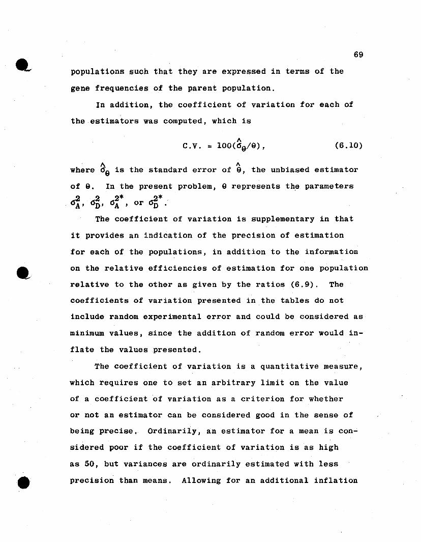
populations such that they are expressed in terms o,f the
gene frequencies of the parent population.
In addition, the coefficient of variation for each of
the estimators was computed, which is
1\C.v. = 100(69/9), (6.10)
1\ 1\where ~9 is the standard error of 9, the unbiased estimator
of 9.
~, ~,
In the present problem, 9 represents the parameters
2* 2*6A ' or 6n .
The coefficient of variation is supplementary in that
it provides an indication of the precision of estimation
for each of the populations, in addition to the information
on the relative efficiencies of estimation for one population
relative to the other as given by the ratios (6.9). The
coefficients of variation presented in the tables do not
include random experimental error and could be considered as
minimum values, since the addition of random error would in-
flate the values presented.
The coefficient of variation is a quantitative measure,
which requires one to set an arbitrary limit on the value
of a coefficient of variation as a criterion for whether
or not an estimator can be considered good in the sense of
being precise. Ordinarily, an estimator for a mean is con-
sidered poor if the coefficient of variation is as high
as 50, but variances are ordinarily estimated with less
precision than means. Allowing for an additional inflation
,--,.
70
of the coefficient of variation due to random error, the
estimators obtained will be considered sufficiently precise
if the coefficient of variation is <40.
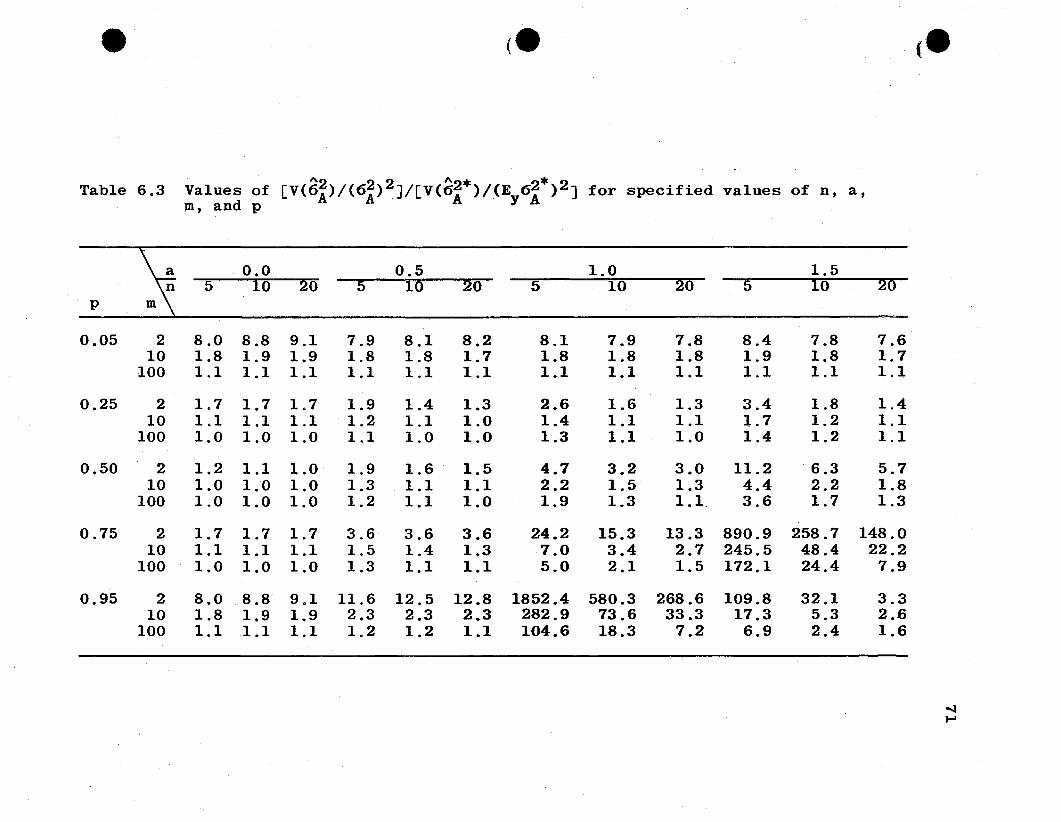
Results on the evaluation of the ratio for additive
variance estimators, (6.9), with specified values of n, a,
m, and p are given in Table 8.3. Values for 1000 loci dif
fer only slightly from those for 100 loci and are eliminated
from the table. Also, results for n=15 are eliminated since
-the trend for increasing n is well illustrated with those
values used in the table. The coefficients of variation for
"2 "2*6A and 6A are shown in Tables 6.4 and 6.5, respectively, for
specified values of n, a, m, and P. It should be noted that
~2*the coefficient of variation for vA is independent of gene
frequency and degree of dominance.
Generally, the derived population estimator is more ef-
ficient than the parent population estimator; and as both m
and n become larger the ratio becomes smaller, as shown in
Table 6.3. Extremely high values of the ratio for some cases
of p=0.75, 0.95 are accounted for by a divergence of the gen-
etic variances of the two populations at these points. Obser-
vation of additive genetic variance for the two populations
in Tables 6.6 and 6.7 reveals additive genetic variance in the
parent population to be much smaller than that of the derived
population at these crucial points, hence causing the ratios
to be very large. An increase in the degree of dominance
appears to accentuate the high and low points in the tables.
e (e (e
Table 6.3 Values of [V(6~)/(6~)2J/[V(6~*)/(E6:*)2J for specified values of D, a,m, and p Y
~0.0 0.5 1.0 1.5
5 10 20 5 10 20 5 10 20 : 10 20P
0.05 2 8.0 8.8 9.1 7.9 8.1 8.2 8.1 7.9 7.8 8.4 7.8 7.610 1.8 1.9 1.9 1.8 1.8 1.7 1.8 1.8 1.8 1.9 1.8 1.7
100 1.1 1.1 1.1 1.1 1.1 1.1 1.1 1.1 1.1 1.1 1.1 1.1
0.25 2 1.7 1.7 1.7 1.9 1.4 1.3 2.6 1.6 1.3 3.4 1.8 1.410 1.1 1.1 1.1 1.2 1.1 1.0 1.4 1.1 1.1 1.7 1.2 1.1
100 1.0 1.0 1.0 1.1 1.0 1.0 1.3 1.1 1.0 1.4 1.2 1.1
0.50 2 1.2 1.1 1.0 1.9 1.6 1.5 4.7 3.2 3.0 11.2 6.3 5.710 1.0 1.0 1.0 1.3 1.1 1.1 2.2 1.5 1.3 4.4 2.2 1.8
100 1.0 1.0 1.0 1.2 1.1 1.0 1.9 1.3 1.1. 3.6 1.7 1.3
0.75 2 1.7 1.7 1.7 3.6 3.6 3.6 24.2 15.3 13.3 890.9 258.7 148.010 1.1 1.1 1.1 1.5 1.4 1.3 7.0 3.4 2.7 245.5 48.4 22.2
100 1.0 1.0 1.0 1.3 1.1 1.1 5.0 2.1 1.5 172.1 24.4 7.9
0.95 2 8.0 8.8 9.1 11.6 12.5 12.8 1852.4 580.3 268.6 109.8 32.1 3.310 1.8 1.9 1.9 2.3 2.3 2.3 282.9 73.6 33.3 17.3 5.3 2.6
100 1.1 1.1 1.1 1.2 1.2 1.1 104.6 18.3 7.2 6.9 2.4 1.6
....:I....
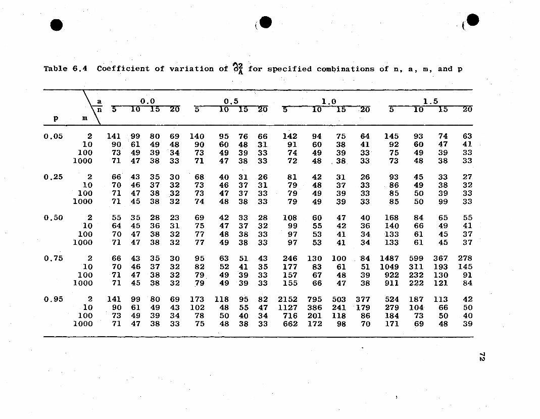
e (e .(e
Table 6.4 Coefficient of variation of ~f for specified combinations of n, a, m, and p
~5 0.0 0.5 1.0 1.510 IS 20 5 10 15 20 5 10 15 .20 5 10 15 20
p
0.05 2 141 99 80 69 140 95 76 66 142 94 75 64 145 93 74 6310 90 61 49 48 90 60 48 31 91 60 38 41 92 60 47 41
100 73 49 39 34 73 49 39 33 74 49 39 33 75 49 39 331000 71 47 38 33 71 47 38 33 72 48 ,38 33 73 48 38 33
0.25 2 66 43 35 30 68 40 31 26 81 42 31 26 93 45 33 2710 70 46 37 32 73 46 37 31 79 48 37 33 86 49 38 32
100 71 47 38 32 73 47 37 33 79 49 39 33 85 50 39 331000 71 45 38 32 74 48 38 33 79 49 39 33 85 50 99 33
0.50 2 55 35 28 23 69 42 33 28 108 60 47 40 168 84 65 5510 64 45 36 31 75 47 37 32 99 55 42 36 140 66 49 41
100 70 47 38 32 77 48 38 33 97 53 41 34 133 61 45 371000 71 47 38 32 77 49 38 33 97 53 41 34 133 61 45 37
0.75 2 66 43 35 30 95 63 51 43 246 130 100 '84 1487 599 367. 27810 70 46 37 32 82 52 41 35 177 83 61 51 1049 311 193 145
100 71 47 38 32 79 49 39 33 157 67 48 39 922 232 130 911000 71 45 38 32 79 49 39 33 155 66 47 38 911 222 121 84
0.95 2 141 99 80 69 173 118 95 82 2152 795 503 377 524 187 113 4210 90 61 49 43 102 48 55 47 1127 386 241 179 279 104 66 50
100 73 49 39 34 78 50 40 34 716 201 118 86 184 73 50 401000 71 47 38 33 75 48 38 33 662 172 98 70 171 69 48 39
'JlI.:)
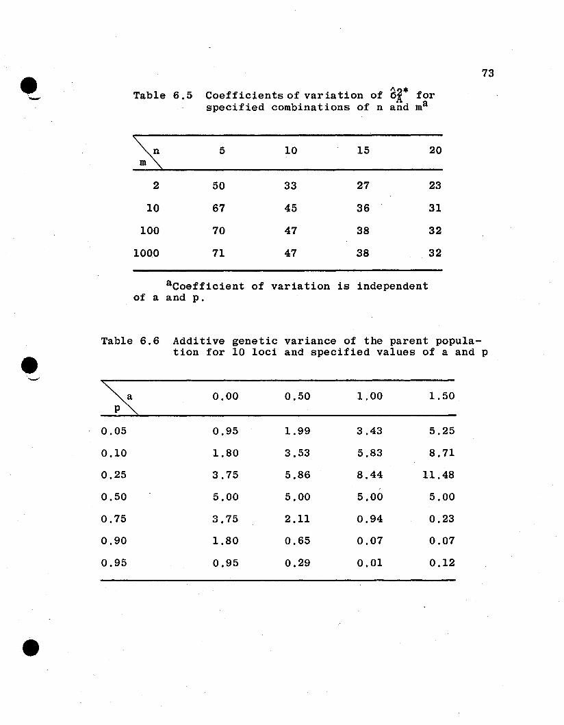
Table 6.6 Additive genetic variance of the parent popula-tion for 10 loci and specified values of a and pe
'-"
~ 0.00 0.50 1.00 1.50
0.05 0.95 1.99 3.43 5.25
0.10 1.80 3.53 5.83 8.71
0.25 3.75 5.86 8.44 11.48
0.50 5.00 5.00 5.00 5.00
0.75 3.75 2.11 0.94 0.23
0.90 1.80 0.65 0.07 0.07
0.95 0.95 0.29 0.01 0.12
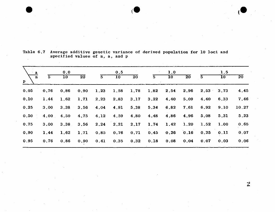
e (e (e
Table 6.7 Average additive genetic variance of derived population for 10 loci andspecified"va1ues of n, a, and p
"a 0.0 0.5 1.0 1.5- 10 20n 5 10 20 5 10 20 5 10 20 5p \0.05 0.76 0.86 0.90 1.23 1.58 1.78 1.82 2.54 2.96 2.53 3.73 4.45
0.10 1.44 1.62 1.71 2.23 2.83 3.17 3.22 4.40 5.09 4.40 6.33 7.46
0.25 3.00 3.38 3.56 4.04 4.91 5.38 5.34 6.82 7.61 6.92 9.10 10.27
0.50 4.00 4.50 4.75 4.12 4.59 4.80 4.48 4.86 4.96 5.08 5.31 5.23
0.75 3.00 3.38 3.56 2.24 2.21 2.17 1.74 1.42 " 1.20 1.52 1.00 0.65
0.90 1.44 1.62 1.71 0.85 0.76 0.71 0.45 0.26 0.16 0.25 0.11 0.07
0.95 0.76 0.86 0.90 0.41 0.35 0.32 0.18 0.08 0.04 0.07 0.03 0.06
'It/:lo.
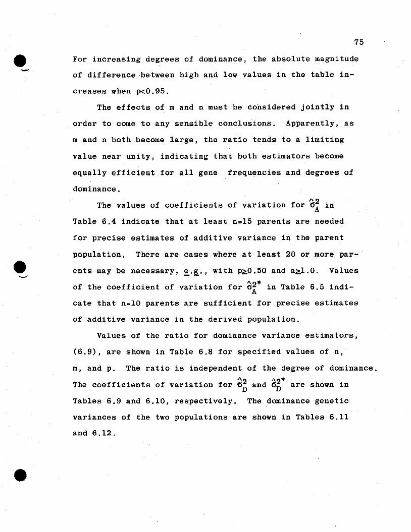
-
\,--,,-
75
For increasing degrees of dominance, the absolute magnitude
of difference between high and low values in the table in-
creases when p<0.95.
The effects of m and n must be considered jointly in
order to come to any sensible conclusions. Apparently, as
m and n both become large, the ratio tends to a limiting
value near unity, indicating that both estimators become
equally efficient for all gene frequencies and degrees of
for precise estimates of additive variance in the parent
population. There are cases where at least 20 or more par-
ents may be necessary, ~.K., with p~0.50 and a~l.O. Values
of the coefficient of variation for d~* in Table 6.5 indi
cate that n=lO parents are sufficient for precise estimates
of additive variance in the derived population.
Values of the ratio for dominance variance estimators,
(6.9), are shown in Table 6.8 for specified values of n,
m, and p. The ratio is independent of the degree of dominance.
"2 A2*The coefficients of variation for 6D
and 6D are shown in
Tables 6.9 and 6.10, respectively. The dominance genetic
variances of the two populations are shown in Tables 6.11
and 6.12.
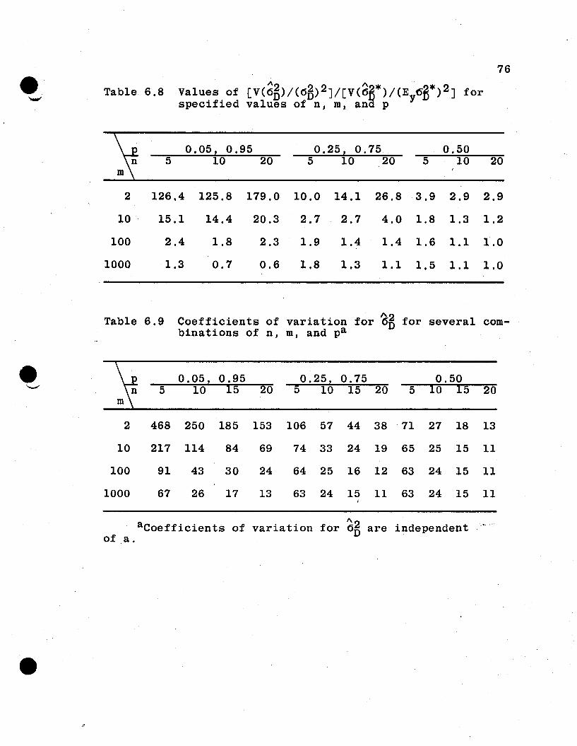
Table 6.8 Values of [V(~~)/(6fi)2J/[V(a~*)/(Ey6~*)2Jforspecified values of n, m, ana p
76
0.05, 0.95 0.25, 0.75 0.505 10 20 5 10 20 5 10 20
2 126.4 125.8 179.0 10.0 14.1 26.8 3.9 2.9 2.9
10 15.1 14.4 20.3 2.7 2.7 4.0 1.8 1.3 1.2
100 2.4 1.8 2.3 1.9 1.4 1.4 1.6 1.1 1.0
1000 1.3 0.7 0.6 1.8 1.3 1.1 1.5 1.1 1.0
Table 6.9 Coefficients of variation for ~fi for several com-binations of n, m, and pa
e 0.05, 0.95 0.25, 0.75 0.50'-' 5 10 15 20 5 10 15 20 5 10 15 20
2 468 250 185 153 106 57 44 38 71 27 18 13
10 217 114 84 69 74 33 24 19 65 25 15 11
100 91 43 30 24 64 25 16 12 63 24 15 11
1000 67 26 17 13 63 24 15 11 63 24 15 11
aCoefficients of variation for "2 are independent _·.--"0.,4.'
6Dof a.
e 77
Table 6.10 Coefficients of variation of "2* for specified'- 6Dvalues of n, m, and pa
~0.05, 0.95 0.25, 0.75 0.50·
5 10 15 20 5 10 15 20 5 10 15 20
2 42 22 15 11 34 15 10 7 36 16 10 8
10 56 30 20 15 45 20 13 10 48 22 14 10
100 59 31 21 16 47 21 14. 10 51 23 15 11
1000 59 32 22 16 47 21 14 10 51 23 15 11
aCoefficients of variation for "2* are independentOnof a.
Table 6.11 Dominance genetic variance of the parent population for 10 loci and specified values ofa and p
•
~a0.05, 0.95
0.10, 0.90
0.25, 0.75
0.50
0.5
0.02
0.08
0.35
0.63
1.0
0.09
0.32
1.41
2.50
1.5
0.20
0.73
3.16
5.63
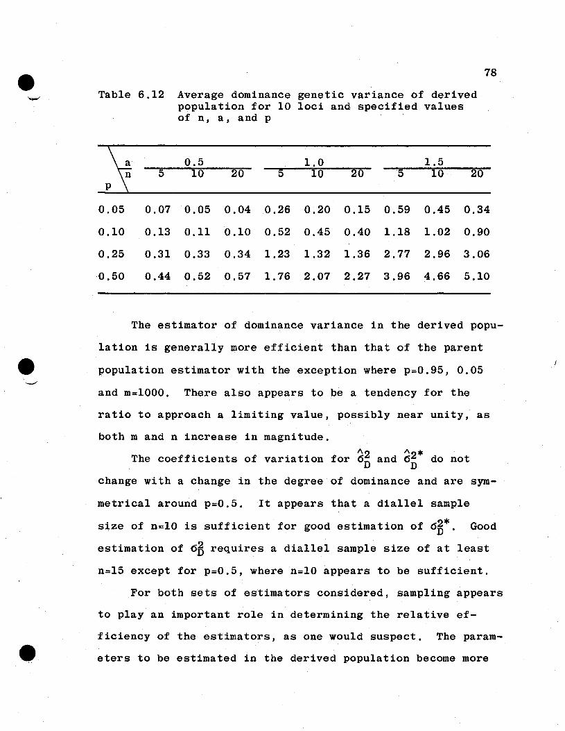
•
The estimator of dominance variance in the derived popu-
lation is generally more efficient than that of the parent
population estimator with the exception where p=0.95, 0.05
and m=1000. There also appears to be a tendency for the
ratio to approach a limiting value, possibly near unity, as
both m and n increase in magnitude.
"2 "2*The coefficients of variation for 6n and 6n do not
change with a change in the degree of dominance and are sym-
metrical around p=0.5. It appears that a diallel sample
size of n=lO is sufficient for good estimation of 6~*. Good
estimation of 6~ requires a diallel sample size of at least
n=l5 except for p=0.5, where n=lO ~ppears to be sufficient.
For both sets of estimators considered, sampling appears
to play an important role in determining the relative ef-
ficiency of the estimators, as one would suspect. The param-
eters to be estimated in the derived population become more
79
like their counterparts in the parent population as the sample
size of the diallel increases; bence, the variances of their
estimators would be expected to become more like those for
the parent population. Also, the number of loci seems to have
an important role and their effect on the relative efficiencies
must be considered jointly with the sample size, as indicated
earlier.
The situations considered may be 'somewhat artificial due
to the physical limitations encountered in the numerical
evaluations. Also, it is highly unlikely that all genes
controlling any character have the same frequency in a popu-
lation or that all loci exhibit the same degree of dominance.
An attempt was made to study the possible effects of this
restriction by considering 10 subsets of 10 loci with vary
ing combinations of the other parameters, n, a, and p. In
all cases considered, the averages over the 10 subsets fell
in the expected region assuming 100 loci with parameters
equal to the average of the 10 subset parameters. Thus, the
assumption of equal parameters in the numerical evaluations
did not appear to be too misleading.
The mean square error of the biased estimators for the
derived population parameters is shown in Table 6.13, let-
ting ui=uj=l, Pi=Pj=P, and ai=aj=a. The mean square error
of an estimator is its .variance plus the square of its bias.
The formulas of Table 6.13 were obtained from the variance
and the bias of each estimator shown in (6.7).
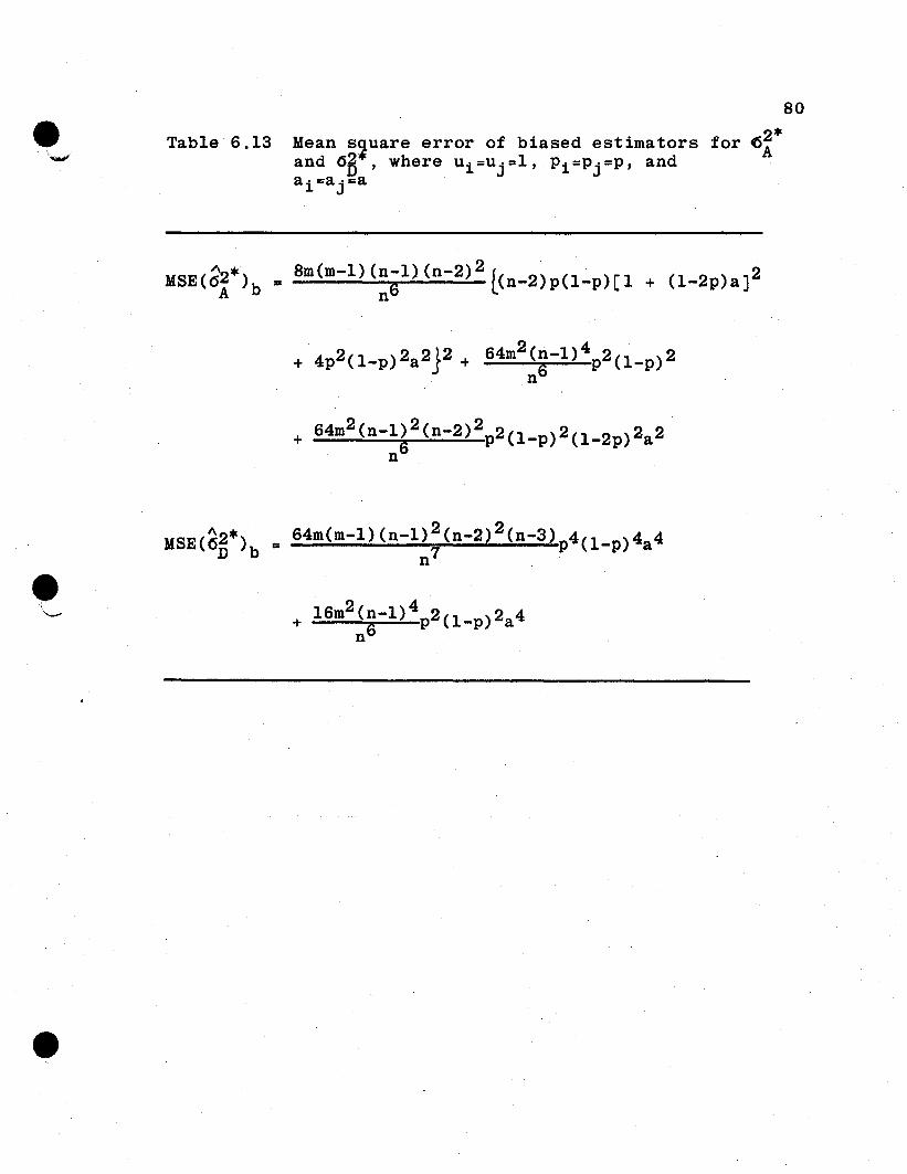
80
Table"6.13 Mean s~uare error of biased estimators for 6~*and On ' where ui:Uj=l, Pi=Pj=P, andai=ajl:a "
MSE(6A2*)b = 8m(m-l)(n-l)(n-2)2 l(n_2)p(1_P)[1 + (1-2p)a]2n6
81
A numerical evaulation of the mean square error of the
biased estimators, the genetic variances of the derived popu-
lation, and the bias of the estimators were made using par-
ticular values of n, a, m, and p. The ratios of the variances
for parent population estimators to the mean square error for
biased derived population estimators were computed.
Table 6.14 illustrates the general results of the in-
vestigation for additive variance estimators. The gene fre-
quencies and degrees of dominace are some of those used in
Table 6.3 for purposes of comparison.
The same general patterns of behavior occurred with the
biased estimators as with the unbiased estimators for the de-
rived population parameters. However, the biased estimators
were less efficient than the unbiased estimators, if the
mean square error was considered as the measure of ,efficiency
for the biased estimators. The efficiency of the biased estima-
tors was also computed using their variance rather than the
mean square. When the variance was used as a measure of ef-
ficiency, the biased estimators had a higher relative ef-
ficiency than did the unbiased estimators.
But the magnitude of the bias associated with the est i-
mator must also be considered. The bias associated with the
biased estimator ranges from roughly 60 percent of the addi
tive variance for n=5 to roughly 25 percent of the additive
variance for n=20.
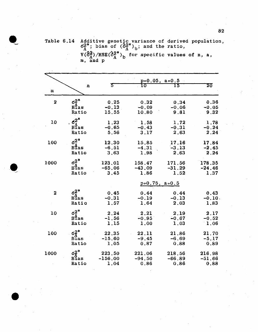
82
tit Table 6.14 Additive genetic variance of derived population,62*. bias of (&~*)b; and the ratio,
A 'V(a2)/MSE(~2*) for specific values of n, a,A A bm, and p
I;:n p=0.05, a=0.55 10 15 20
2 0'2* 0.25 0.32 0.34 0.36ABlas -0.13 -0.09 -0.06 -0.05Ratio 15.55 10.80 9.81 9.32
10 "2* 1.23 1.58 1.72 1.78• 6ABlas -0.65 -0.43 -0.31 -0.24Ratio 5.56 3.17 2.63 2.24
100 62* 12.30 15.85 17.16 17.84Bias -6.51 -4.31 -3.13 -2.45Ratio 3.63 1.98 2.63 2.24
1000 2* 123.01 158.47 171.56 178.35
•••O'ABlas -65.06 -43.09 -31.29 -24.46Ratio 3.45 1.86 1.52 1.37
p=0.75, a=0.5
2 62* 0.45 0.44 0.44 0.43ABlas -0.31 -0.19 -0.13 -0.10,Ratio 1.57 1.64 2.03 1.83
10 6 2* 2.24 2.21 2.19 2.17Bias -1.56 -0.95 -0.67 -0.52Ratio 1.15 1.00 1.03 1.06
100 6i* 22.35 22.11 21.86 21.70Blas -15.60 -9.45 -6.69 -5.17Ratio 1.05 0.87 0.88 0.89
1000 6H* 223.50 221.06 218.56 216.98Blas -156.00 -94.50 -66.89 -51.66Ratio 1.04 0.86 0.86 0.88
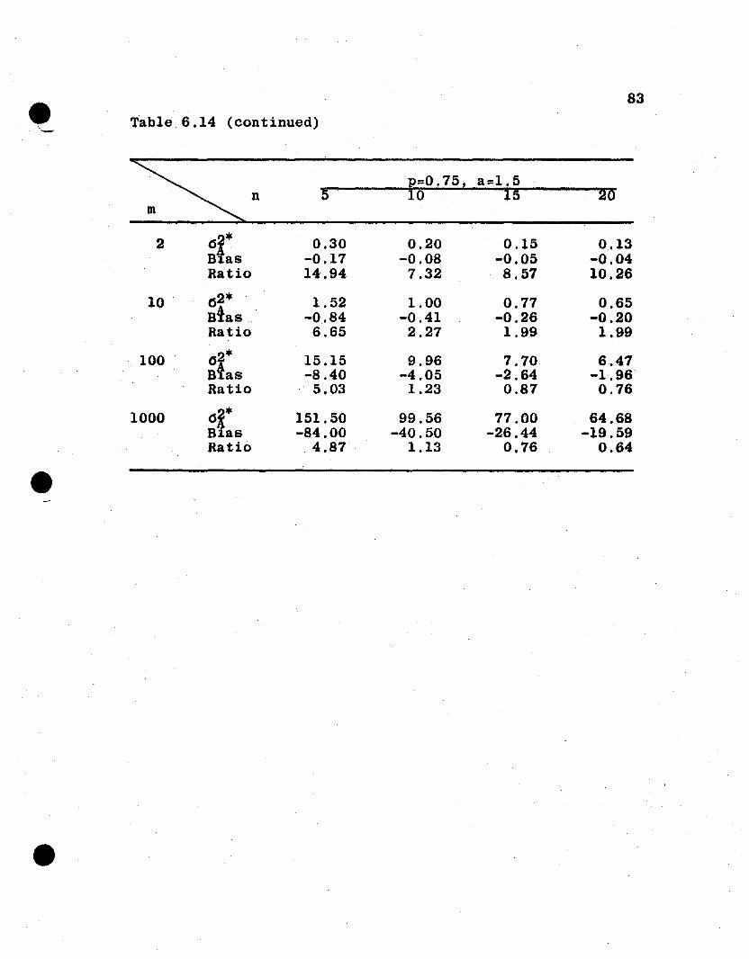
e 83
Table 6.14 (continued)''<-..-.'
S':n p=0.75, a=1.55 10 15 20
2 62* 0.30 0.20 0.15 0.13Btas -0.17 -0.08 -0.05 -0.04Ratio 14.94 7.32 8.57 10.26
10 .' 02* . 1.52 1.00 0.77 0.65Bias . -0.84 -0.41 -0.26 -0.20Ratio 6.65 2.27 1.99 1.99
100 o~* 15.15 9.96 7.70 6.47B as -8.40 -4.05 -2.64 -1.96Ratio 5.03 1.23 0.87 0.76
1000 o~* 151.50 99.56 77.00 64.68B1.as -84.00 -40.50 -26.44 -19.59Ratio . 4.87 1.13 0.76 0.64
e
•
84
The biased dominance variance estimators for the de-
rived population parameters produced results similar to
the biased additive variance estimators (Table 6.15). In
all cases, the biased estimators were less efficient than
the unbiased estimators with the mean square error com-
parison. If the variance of the biased estimator was used
as an efficiency measure, the biased estimators were more
efficient than the unbiased estimators" .However , the bias
of the dominance variance estimator was roughly 80 percent
of 62* for n=5 to roughly 30 percent of 62* for n=20.D D
The unbiased estimators for derived population param-
eters would be more desirable for use than the biased esti-
mators, since they are more efficient. Also, the bias
associated with the biased estimators is quite large, and
it seems to be relatively easy to correct for the bias by
the use of information from the parental analysis.
6.5 Consequences of Random Experimental Error
6.5.1 Parent Population Estimators. The estimators
and their variances shown in Section 6.1 pertain to the
genetic portion of the model and ignore any random contribu-
tion due to experimental error. In this section, the change
in estimators from the dia1le1 and their variances upon in-
elusion of random experimental error for the strictly addi-
tive and dominance genetic model in the absence of epistasis
are indicated.
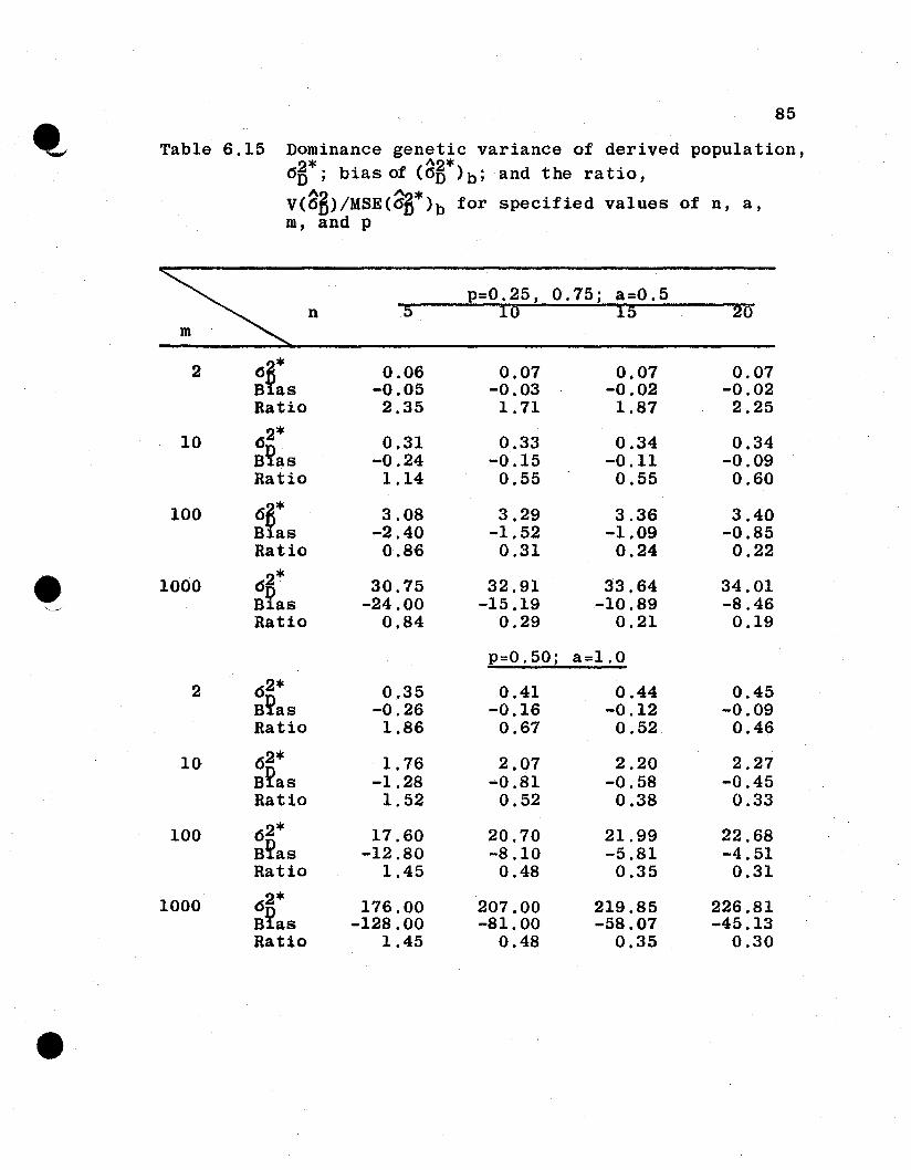
85
~ Table 6.15 Dominance genetic variance of derived population,2* "2* and the ratio,6n ; bias of (OD )b;
V(a~)/MSE(~*)b for specified values of n, a,m, and p
S p=0.25, 0.75; a=0.5n 5 10 15 20
2 ~~:s 0.06 0.07 0.07 0.07-0.05 -0.03 -0.02 -0.02
Ratio 2.35 1.71 1.87 2.25
10 2* 0.31 0.33 0.34 0.346B~as -0.24 -0.15 -0.11 -0.09Ratio 1.14 0.55 0.55 0.60
100 6B* 3.08 3.29 3.36 3.40Blas -2.40 -1.52 -1.09 -0.85Ratio 0.8,6 0.31 0.24 0.22
e 1000 2* 30.75 32.91 33.64 34.016J;)Blas -24.00 -15.19 -10.89 -8.46Ratio 0.84 0.29 0.21 0.19
p=0.50; a=1.0
2 6 2* 0.35 0.41 0.44 0.45B~as -0.26 -0.16 -0.12 -0.09Ratio 1.86 0.67 0.52 0.46
10 62* 1.76 2.07 2.20 2.27nBlas -1.28 -0.81 -0.58 -0.45Ratio 1.52 0.52 0.38 0.33
100 6 2* 17.60 20.70 21.99 22.68B~as -12.80 -8.10 -5.81 -4.51Ratio 1.45 0.48 0.35 0.31
1000 62* 176.00 207.00 219.85 226.81B£as -128.00 -81.00 -58.07 -45.13Ratio 1.45 0.48 0.35 0.30
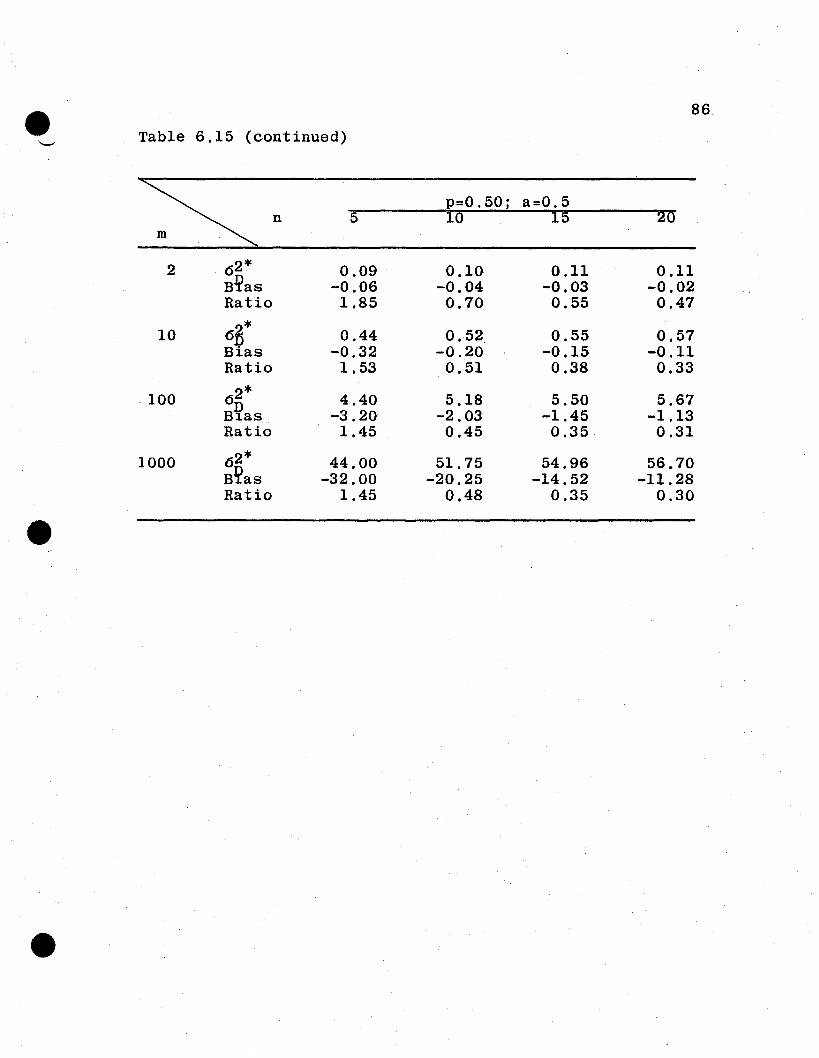
e 86
Table 6.15 (continued)"-
S p=0.50; a=0.5n 5 10 15 20
2 6 2* 0.09 0.10 0.11 0.11Blfas -0.06 -0.04 -0.03 -0.02Ratio 1.85 0.70 0.55 0.47
10 6~* 0.44 0.52 0.55 0.57Bias -0.32 -0.20 -0.15 -0.11Ratio 1.53 0.51 0.38 0.33
" 100 2* 4.40 5.18 5.50 5.676DBl.as -3.20 -2.03 -1.45 -1.13Ratio 1.45 0.45 0.35 0.31
1000 62* 44.00 51.75 54.96 56.70B£as -32.00 -20.25 -14.52 -11.28Ratio 1.45 0.48 0.35 0.30
e
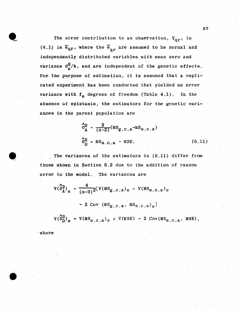
•
87
The error contribution to an observation, YqrJ in
(4.1) is eqr , where the eqr are assumed to be normal and
independently distributed variables with mean zero and
v~riance 62/k, and are independent of the genetic effects.e
For the purpose of estimation, it is assumed that a rep1i-
cated experiment has been conducted that yielded an error
variance with f e degrees of freedom (Table 4.1). In the
absence of epistasis, the estimators for the genetic vari-
ances in the parent population are
(6.11)
The variances of the estimators in (6.11) differ from
those shown in Section 6.2 due to the addition of random
error to the model. The variances are
A2V(6n)e = V(MSs.c.a)e + V(MSE) - 2 Cov(MSs . c . a ' MSE) ,
where
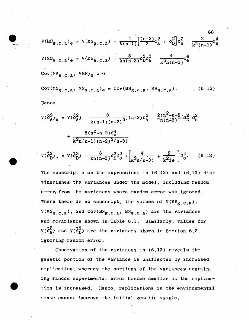
e'-
~ V(MS g . c . a ) + 4 [(n-2)6A2 +k(n-1) 2
(6.12)
Cov(MSs,c.a' MSE)e ~ 0
Cov(MSg . c . a ' MSs.c.a)e = Cov(MSg . c . a , MSs . c . a )·
Hence
2+ 8 [(n-2)62 + 2(n -n-2)62 J62
k(n-1)(n-2)2 A n(n-3) D e
8(n2-n-2)6~+
k 2n(n-1) (n-2)2(n-3)
(6.13)
The subscript e on the expressions in (6.12) and (6.13) dis-
tinguishes the variances under the model, including. random
erro~ from the variances where random error was ignored.
Where there is no subscript, the values of V(MSg . c . a ),
V(MSs . c . a )' and Cov(MSg . c . a , MSs . c . a ) are the variances
and covariance shown in Table 6.1. Similarly, values for
V(~) and v(2~) are the variances shown in Section 6.2,
ignoring random error.
Observation of the variances in (6.13) reveals the
genetic portion of the variance is unaffected by increased
replication, whereas the portions of the variances contain-
ing random experimental error become smaller as the replica-
tion is increased. Hence, replications in the environmental
sense cannot improve the initial genetic sample.
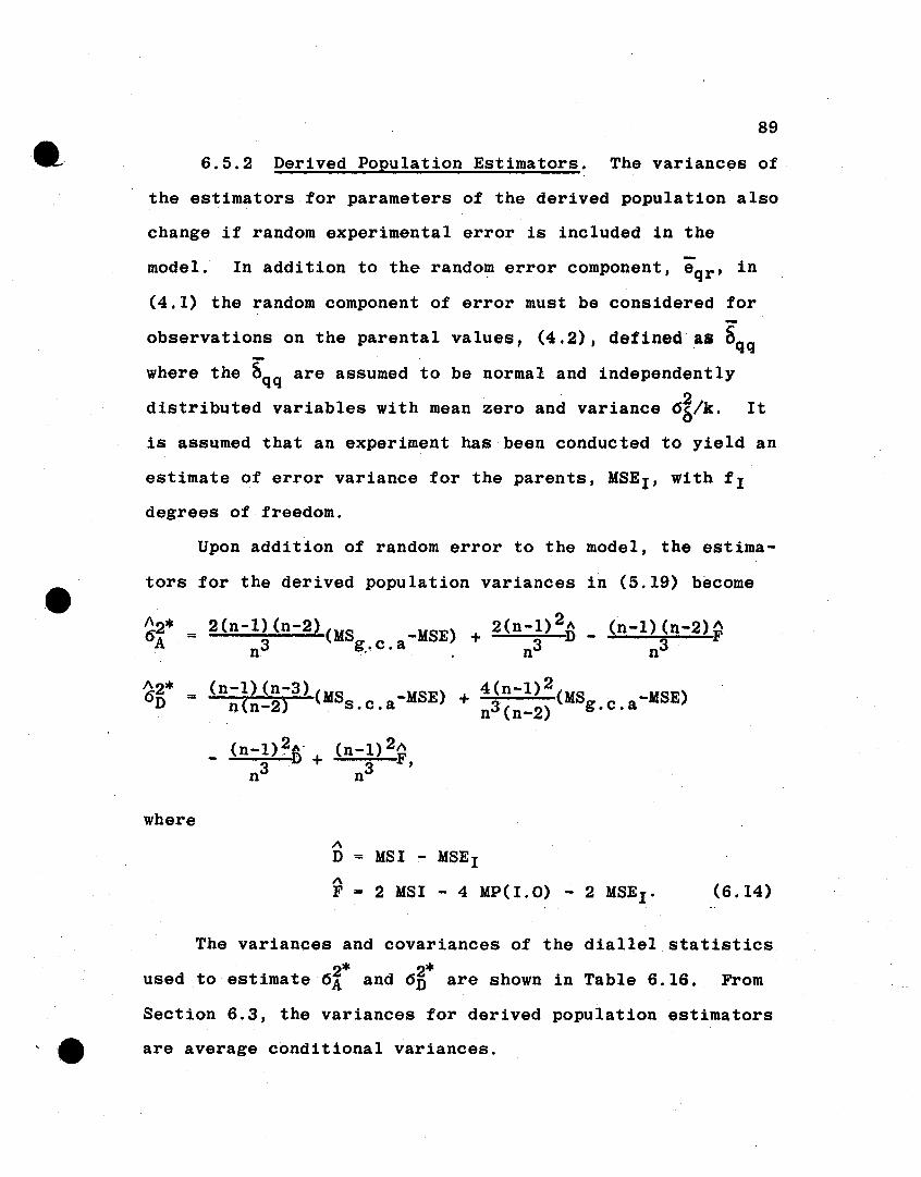
89
6.5.2 Derived Population Estimators. The variances of
the estimators for parameters of the derived population also
change if random experimental error is included in the
model. In addition to the random error component, eqr , in
(4.1) the random component of error must be considered for-
observations on the parental values, (4.2), defined as Sqq
where the aqq are assumed to be normal and independently. 2
distributed variables with mean zero and variance 6b/k. It
is assumed that an experiment has been conducted to yield an
estimate of error variance for the parents, MSE I , with f I
degrees of freedom.
Upon addition of random error to the model, the estima-
tors for the derived population variances in (5.19) become
~D2* (n-l)(n-3)(MS -MSE) + 4(n-l)2(MS -MSE)n(n-2) s.c.a n3 (n-2) g.c.a
(n-I) ?,.. (n-l) 2"- D + 3 F,
n3 n
where1\D = MSI - MSE I1\F = 2 MSI - 4 MP(I.O) - 2 MSE I . (6.14)
'e
The variances and covariances of the dial leI statistics
2* 2*used to estimate 6A and 6D are shown in Table 6.16. From
Section 6.3, the variances for derived population estimators
are average conditional variances.
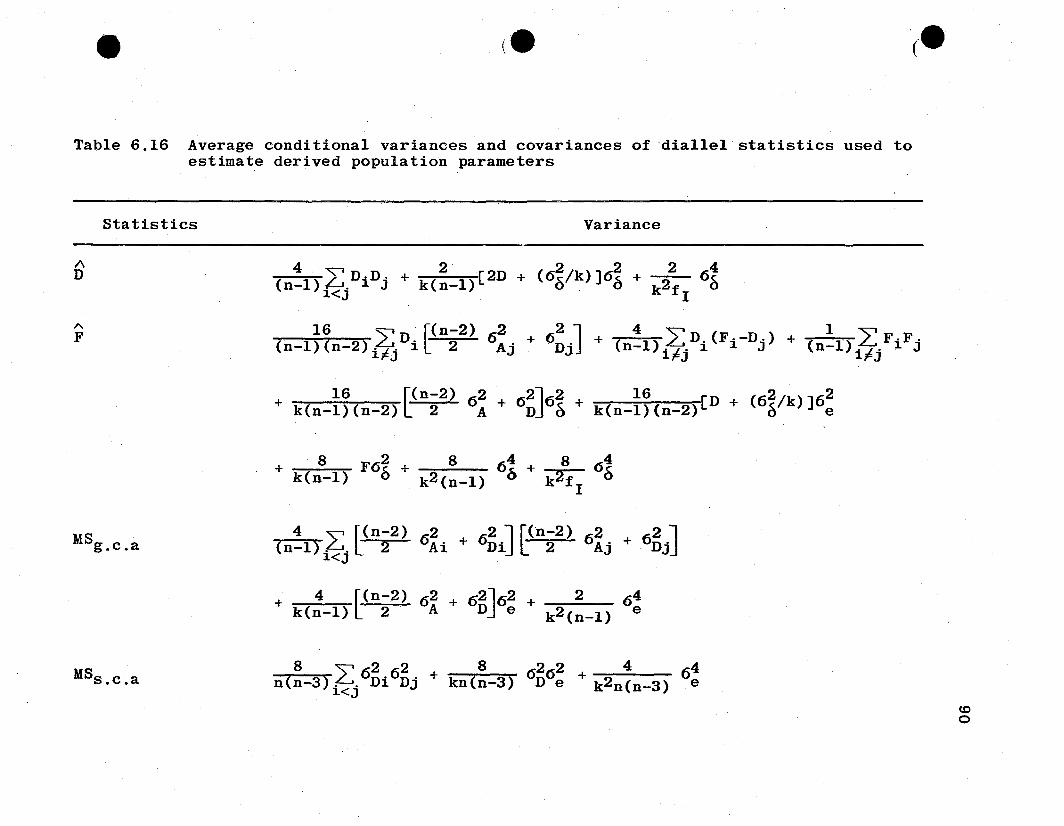
e (e .(e
Table 6.16 Average conditional variances and covariances of ·diallel statistics used toestimate derived population parameters
Statistics
/\D
A
F
MSg . c . a
MSs •c •a
Variance
4 "'V 2 2 2 2 4-. ~~oDiDj + k( -1) [2D + (6e5/k) ]6() + -2- 6:)
~<J n . k f I
16 ~ [(n-2) 2 21 4"" 1 ""V(n-l)(n-2)~oDi[ 2 6AJo + 6DJ
o + (n_l)~oDi(Fi-Dj) + (n_l)~.FiFj~FJ . ~FJ ~FJ
16 [(n-2) 2 2J 2 16 2 2+ k(n-l)(n-2)[ 2 6A + 6D 6 6 + k(n-l) (n_2)[D + (6:)/k)]6e
+ 8 F62 + 8 64 + 8 64k(n-l) 6 k2 (n-l) 0 k2f
I0
4 "'"' L(n-2) 2 2 JrJn-2) 2 2 ]; ~ < &j [ . 2 6Ai + 6Di [2 6Aj + 6Dj
+ 4 [(n-2) 62 + 62J62 + 2 64k(n-l) L 2 A D e k2 (n-l) e
8 "'"' 62 62 + 8 6262 + 4 64n(n-3)~. Di Dj kn(n-3) D e k2n(n-3) e
~<J
coo
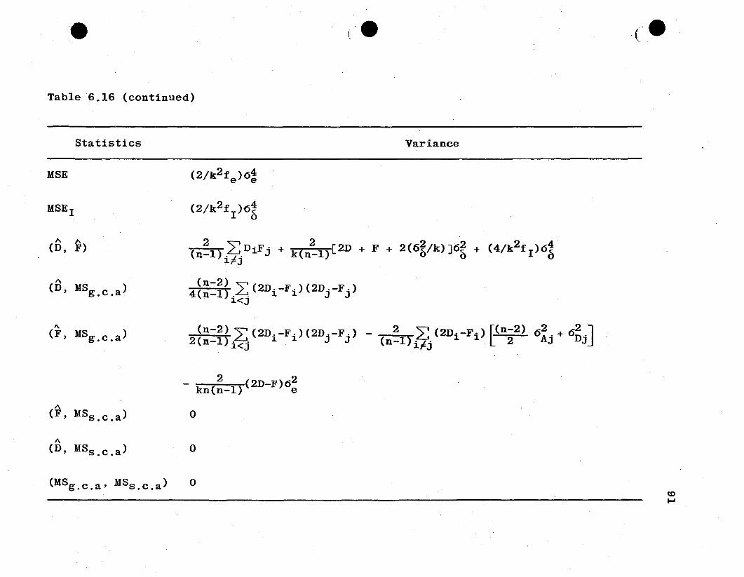
'e
Table 6.16 (continued)
(oe ore
Statistics
MSE
MSE 1
" A(D, F)
1\(D, MSg . c . a )
"(F, MSg . c . a )
(F, MSs • c •a )
(D, MSs . c . a )
(MSg . c . a , MSs . c . a )
Variance
(2/k2 f )64e e
(2/k2 f )64I b
2 '" 2 2 2 2 4. -- o~.DiFj + k(n_l)[2D + F + 2(6b/k)]6& + (4/k f I )6blr=J
(n-2) ~ ( ) ( ).• ~,.~2Di-Fi 2Dj -Fjl<J
(n-2) "" (2D. -F.) (2D .-F.) - 2 ~ (2D· -F·) [(n-2) 6 2 . + 6 2 .J2(n-l)i~ 1 1 J J (n-l)i~j 1 1 [2 AJ DJ
-. ,2 ~ , (2D-F) 6~
o
o
o(D....
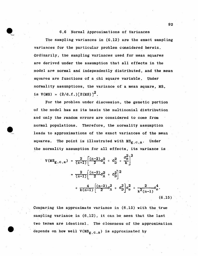
92
6.6 Normal Approximations of Variances
The sampling variances in (6.12) are the exact sampling
variances for the particular problem considered herein.
Ordinarily, the sampling variances used for mean squares
are derived under the assumption that all effects in the
model are normal and independently distributed, and the mean
squares are functions of a chi square variable. Under
normality assumptions, the variance of" a mean square, MS,
is V(MS) = (2/d.f.)[E(MS)]2.
For the problem under discussion, the genetic portion
of the model has as its basis the multinomial distribution
and only the random errors are considered to come from
normal populations. Therefore, the normality assumption
leads to approximations of the exact variances of the mean
squares. The point is illustrated with MSg . c . a ' Under
the normality assumption for all effects, its variance is
V(MSg •c •a ) = 2 f(n-2)62 + 62 + 6~]2(n-l)l 2 A D ~
= 2 [(n-2) (52 + 6D2l2(n-l) 2 A IJ
+ 4 [(n-2)62 + 6D2JOe2 + 2 64
k(n-l)[ 2 A k2 (n-l) e'
(6.15)
Comparing the approximate variance in (6,15) with the true
sampling variance in (6.12), it can be seen that the last
two terms are identical. The closeness of the approximation
depends on how well V(MSg,c.a) is approximated by
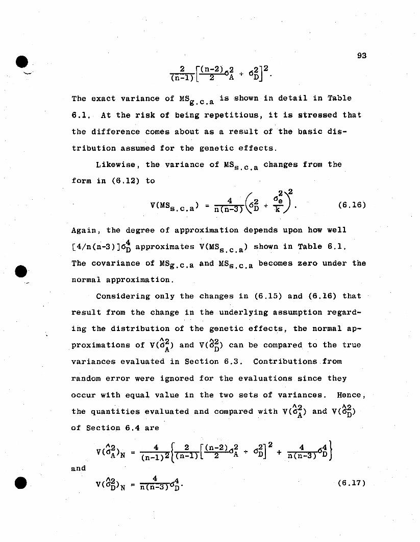
93
2 r(n-2)o2 (2)2(n-l)l 2 A +n .
The exact variance of MSg . c . a is shown in detail in Table
6.1. At the risk of being repetitious, it is stressed that
the difference comes about as a result of the basic dis-
tribution assumed for the genetic effects.
Likewise, the variance of MSs . c . a changes from the
form in (6.12) to
4 (2 0:)2V(MSs . c •a ) = n(n-3)~n + ~ . (6.16)
Again, the degree of approximation depends upon how well
[4/n(n-3)]6~ approximates V(MSs . c . a ) shown in Table 6.1.
The covariance of MSg . c . a and MSs . c . a becomes zero under the
hormal approximation.
Considering only the changes in (6.15) and (6.16) that
result from the change in the underlying assumption regard
ing the distribution of the genetic effects, the normal ap
proximations of V(6~) and V(a~) can be compared to the true
variances evaluated in Section 6.3. Contributions from
random error were ignored for the evaluations since they
occur with equal value in the two sets of variances. Hence,
the quantities evaluated and compared with V(~~) and V(~~)
of Section 6.4 are
4 f 2 [ (n-2 ) 0 2 2] 2 4 4 }= (n-l)2 (n-l) 2 A + On + n(n_3)60
and
(6.17)
94
The subscript N in (6,17) distinguishes the normal approxi-
mations to the variances from the true variances as evalu-
ated in Section 6.4.
The variances in (6.17) were evaluated in the same man-
ner as outlined in Section 6.4. The following ratios were
then computed.
(6.18 )
A2 A2 ~2where V(6A)N and V(6n)N are shown in (6.17) and V(6A) and
V(~~) were evaluated in Section 6.4. The normal approxi~
mations of the variances are too low if the ratios in (6.18)
are <1 and too high if the ratios are >1.
Some of the results are presented in Table 6.17 to il-
lustrate the general pattern of behavior of the ratio of
the two variances for the estimator of additive genetic vari-
ance. The most obvious development is that the normal ap-
proximation appears to be very good with a large number of.
loci, malOO, for all gene frequencies and degrees of domi-
nance. When the value of m is low, several trends are evi-
dent. First, the normal variance underapproximates the
true variance for low and high gene frequencies, while it
overapproximates at intermediate gene frequencies and low
degree of dominance. An increase of the degree of dominance
results in a decrease of the normal approximation relative
to the true variance, in most cases. The results.for a=O.5
are similar to those for a=O.O and the results for a=1.5
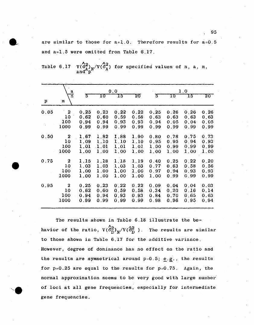
95
a, are similar to those for a'""LO. Therefore results for a==0.5
and a::::l.5 were omitted from Table 6.17.
Table 6.17 "2 ~ for specified values ofV(6A)N/V ( A) n, a, m,and p
~0.0 1.0
5 10 15 20 S 10 15 20p
0.05 2 0.25 0.23 0.22 0.22 0.25 0.26 0.26 0.2610 0.62 0'.60 0.59 0.58 0.63 0.63 0.63 0.63
100 0.94 0.94 0.93 0.93 0.94 0.05 0.04 0.051000 0.99 0.99 0.99 0.99 0.99 0.99 0.99 0.99
0.50 2 1.67 1.82 1.88 1.90 0.80 0.78 0.75 0,7310 1.09 1.10 1.10 1.10 0.95 0.95 0.94 0.93
100 1.01 1.01 1.01 1. 01 1.00 0.99 0.99 0.991000 1.00 1.00 1.00 1.00 1.00 1. 00 1.00 1. 00
0.75 2 1.15 1.18 1.18 1.19 0.40 0.25 0.22 0.2010 1.03 1.03 1.03 1.03 0.77 0.63 0.58 0.56
100 1.00 1.00 1.00 1.00 0.97 0.94 0.93 0.931000 1.00 1.00 1.00 1.00 1. 00 0,99 0.99 0.99
0.95 2 0.25 0.23 0.22 0.22 0.09 0.04 0.04 0.0310 0.62 0.60 0.59 0.58 0.34 0.20 0.16 0.14
100 0.94 0.94 0.93 0.93 0.84 0.70 0.65 0.631000 0.99 0.99 0.99 0.99 0,98 0.96 0.95 0.94
The results shown in Table 6.18 illustrate the be
havior of the ratio, V(a~)N/V(~). The results are similar
to those shown in Table 6.17 for the additive variance.
However, degree of dominance has no effect on the ratio and
the results are symmetrical around p:.::0.5;£..g., the results
for p::::0.25 are equal to the results for p=0.75. Again, the
normal approximation seems to be very good with large number
of loci at all gene frequencies, especially for intermediate
gene frequencies.
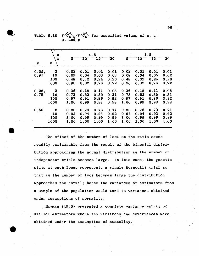
that as the number of loci becomes large the distribution
approaches the normal; hence the variances of estimators from
a sample of the population would tend to variances obtained
under assumptions of normality.
Hayman (1960) presented a complete variance matrix of
diallel estimators where the variances and covariances were.
obtained under the assumption of normality.
--,'
e,
97
7. SUMMARY AND CONCLUSIONS
7.1 Discussion
Most variance estimation procedures in quantitative
genetics are based on the assumption that the experimental
material is a random sample from the population of inference.
Sometimes, however, it is desirable to 'make inferences to a
population that is wholly derived in some prescribed way
from the parents of the experimental material. The use of a
reference base population derived wholly from the parents of
a diallel cross has been studied in this investigation for
the estimators of genetic variance that may be obtained from
the diallel experiment.
Certain assumptions were imposed on the developments
contained herein. In all cases, regular diploid Mendelian
'inheritance was assumed, and both the parent population and
derived population were assumed to be in linkage equilibrium.
The effects of finite sampling from the parent population
were taken into consideration in the development. However,
the development of the random mating derived population was
assumed to proceed in such a manner that random drift was
unimportant. Initially, the genetic model included additive,
dominance, and additive-by-additive epistatic gene effects
" with two alleles at each of two loci. The genetic model was
extended to include an arbitrary number of loci and alleles
in the 'absence of epistasis. The genetic model must be
98
restricted if genetic variances are to be estimated from
the diallel experiment. The usual genetic model assumed for
the diallel analysis is the additive and dominance model in
the absence of epistasis. In some populations, however,
dominance variance may have no significance. And in these
cases the additive and additive-by-additive epistatic genetic
model can be considered.
Unbiased estimators of genetic variances of the parent
population are available from the diallel analysis consisting
of only the Fl crosses either in the absence of dominance or
in the absence of epistasis. Analysis of the inbred parents
is not required for estimation of genetic variances in the
parent population, nor does it aid in the estimation of these
variances--a well-known result.
Unbiased estimators of the genetic parameters in the
derived population under the additive and additive-by-additive
epistatic model were obtained that required no information
on the parents. For the additive and dominance genetic model
in the absence of epistasis, however, it was necessary to use
information from the analysis of the inbred parents to obtain
unbiased estimators of the derived population parameters.
The estimators for the genetic variances in the derived
populations were obtained in such a manner that they were
unbiased with respect to the particular subset of diallel
samples that give rise to the same derived population. That
is, the conditional expectations of the estimators are equal
-'
e·
99
to the genetic variances of the particular derived popula
tion that will be formed from that set of diallel parents,
which implies that the estimators are also unbiased with re-
spect to their unconditional expectations. Also in the
absence of epistasis the mean for a specific derived popula-
tion can be estimated without genetic error from the dial leI
experiment. The mean is the only parameter that can be esti-
mated without genetic error.
The complexity of the exact variances of the estimators
of the derived and parent population parameters ruled out
any analytical comparison of their relative efficiencies.
Consequently, numerical evaluations of the variances and
coefficients of variation of the estimators were made for
the additive and dominance genetic model in order to obtain
information on the usefulness of the derived population
estimators relative to the parent population estimators.
With few exceptions, the estimators for derived popu-
lation parameters were relatively more efficient than esti-
mators for parent population parameters for the cases in-
vestigated in the numerical analysis. There was an indica-
tion that the estimators became equally efficient or nearly
so for large numbers of parents and large numbers of loci
considered jointly, especially at intermediate gene frequencies.
For populations with intermediate gene frequencies, the
method of estimating parameters of the derived population is
recommended. If gene frequencies tend to the extremes, there
•
100
are cases where use of the derived population base may not
be appropriate. However, this is also true for the parent
population base, depending on conditions of the other param
eters, !.~., number of loci and degree of dominance.
Consideration of the results on the coefficients of
variation indicate the need for at least fifteen or more
parents for the diallel to obtain good estimators for the
parent population reference base. The use of ten parents is
. sufficient to obtain the same degree of precision in esti
mating derived population parameters.
It would be desirable in some cases to be able to pro
vide estimates of the derived population parameters from
the information contained only in the analysis of the Fl
crosses. For the additive and dominance genetic model such
estimators must necessarily be biased. However, if the
bias is not too large, the advantage of not having to use
parental information might outweigh the slight bias in
volved.
For this reason, biased estimators for the derived
population parameters were provided for the additive and
dominance genetic model, which included information from
the analysis of the Fl crosses only. Using mean square
error as a measure of their efficiencies, it was found that
the biased estimators were less efficient than the unbiased
estimators. In addition, the bias of the estimators for
genetic variances was very larg,e, varying around 25 percent
101
for the additive variance and around 30 percent for the
dominance 'variance, when n=20. The bias became larger when
n, the number of parental lines, was reduced. In view of
the large bias and the large error mean square, the estima
tion for this'model without parental information was con-
sidered useless.
The exact sampling variances of estimators for addi-
tive and dominance variance in the parent population were
. compared to their normal approximations ordinarily used.
A numerical analysis of the two sets of variances showed
that the variances used under normality assumptions provid-
ed very good approximations to the exact variances and
warranted their use in the analysis. The approximations
were especially good for large numbers of loci and inter-
mediate gene frequencies. The approximations were poor
when 2 or 10 loci were involved and especially so when
gene frequencies were near 0.05 or 0.95.
Comstock and Robinson (1951) obtained experimental
results on the estimates of components of variance from a
series of quantitative genetical experiments on corn. They
compared the dispersion of observed mean squares with that
expected from normal theory and concluded that the assump-
tion of normality was realistic for the material with which
they were working.
102
There is also a considerable savings in time and effort
if the normal approximations are used as opposed to the exact
variances. The derivation of the exact variances is a com-
p1icated and cumbersome operation as compared to the deri-
vation of the normal approximations.
If one accepts the normal approximations to estimator
variances, the difficulties encountered in determining good
estimators for any reference base are reduced considerably.
For the present, consider the derived population reference
base. Following the procedures set forth in Section 5.3.1,
the average values of derived population parameters may be
expressed as linear functions of the parent population
parameters. Estimators for the functions are obtained from
the diallel analysis. The estimators obtained for the average
values of the derived population parameters are unbiased
over those diallel samples that give rise to the same derived
population. The variances of the estimators can be obtained
from the analysis of the diallel cross under the assumption
of normality in the linear model. Where the variance of a2
mean square, MS, will be V(MS)=2[E(MS)] Id.f. With the
assumption of normality, there is no need to obtain the
formula expressing mean squares in terms of sampling varia-
bles and genetic values (Section 4) that were used primarily
to derive the true variances. These results hold for the
additive and dominance genetic model for any number of loci,
,It each with an arbitrary number of alleles.
103
The problem considered herein is not the same as the
case where a plant breeder takes a set of available lines and
uses them in a diallel experiment to estimate derived pop
ulation parameters. The above case calls for exact estimators
in the sense that there is no genetic error of estimation.
In the absence of the ability to develop exact estimators,
the distribution of the diallel samples giving rise to
identical derived populations must be considered in order to
determine expectations of the estimators and variances of the
estimators. The distribution of the diallel samples in this
problem are based on the idea of sampling the parents from
some parent population. Selection or other forces in the
development of a specific set of lines may upset the
assumption of independence of gene distributions necessary
in the development of the results contained herein.
Questions arise as to whether or not the equilibrium
derived population is a realistic reference base or if the
equilibrium population can be attained in practice. Theoret-
ically, of course, the answer to both questions is yes. In
practice, linkage and random drift due to finite samples can
cause some difficulty in approaching an equilibrium pop-
ulation for which genetic variances can be defined. Linkages
slow up the approach to equilibrium and finite populations
introduce the problem of gene fixation and inbreeding. These
forces are discussed earlier in regard to the present problem.
104
The composition of synthetic populations as reservoirs
of genetic variability offer an example of derived popula
tions, provided the original parents of the population are
chosen such that the assumptions listed above are not vio
lated. Although synthetics are best suited for naturally
cross-pollinating species, they can be maintained with cer
tain self-pollinating species such as tobacco where artifi
cial cross-pollinating is easily accomplished.
The selection potential of a population could be evalu-
ated prior' to its synthesis. Ordinarily, the genetic po-
tential of the experimental material would be evaluated
relative to some parent population. However, with the tech-
niques of estimating genetic variances for a derived popula-
tion, the genetic variability could be predicted for the
specific population derived from the experimental material.
The technique of estimating genetic variances for de-
rived populations is highly recommended for use in obtaining
knowledge of the gene action in plant populations, as de-
rived populations are more representative of the real situa-
tion in breeding programs. The potential of this method of
estimation should be investigated further both theoretically
and with actual experimentation. Some suggested extensions
on the problem are presented in Section 7.2.
7.2 Suggestions for Further Research
A number of extensions of the genetic model should be
·tt considered for the use of the derived population as a

105
referenc~ base for the analysis of mating designs. Certainly
efforts should be made to refine the estimation techniques in
order to include ~ore ~eneral epistatic effects with an
arbitrary number of loci and alleles. 'Perhaps an approach
similar to that used in Section 5.3.1 would provide such an
extension. Further elucidations on the effects of linkage
disequilibrium in the derived population and the effects of
random drift in forming the derived population are in order.
The consideration of arbitrary inbreeding of the parents
would broaden the choice of mating designs one could utilize
for inferences to the derived population reference base.
It would also be desirable to have the technique fit
into the framework of covariances of relatives, such that the
covariances obtained from the" mating design could be trans-
lated directly into genetic variances appropriate for the
derived population. Such a transition would simplify exten-
sions to other mating designs.
It appears that many of the extensions to generalize the
genetic model and use of different mating designs might be
accomplished through techniques introduced in Section 5.3.1.
Efforts in the direction of generalizing the method contained
therein may prove to be fruitful.
8. LIST OF REFERENCES
Cockerham, C. C. 1954. An extension of the concept of partitioning hereditary variance for analysis of covariancesamong relatives when epistasis is present. Genetics 39:859-882.
Cockerham, C. C. 1963. Estimation of genetic variances,pp. 53-94. In W. D. Hanson and H. F. Robinson (ed.),Statistical Genetics and Plant Breeding. NationalResearch Council Publication 982, National Academy ofScience, Washington, D.C.
Comstock, R. E., and Robinson, H. F. 1948. The components ofgenetic variance in populations of biparental progeniesand their use in estimating the average degree ofdominance. Biometrics 4:254-266.
Comstock, R. E., and Robinson, H. F .. 1951. Consistency ofestimates of variance components. Biometrics' 7:75-82.
Dickinson, A. G., and Jinks, J. L.'analysis of diallel crosses.
1956. A generalizedGenetics 4l~65-78.
Gilbert, N. E. G. 1958. Diallel cross in plant breeding.Heredi ty 12:0477-492.
Griffing, B. 1956. A generalized treatment of the use ofdiallel crosses in quantitative inheritance. Heredity10:31,:,,50.
Griffing, B. 1958. Application of sampling variables in theidentification of methods which yield unbiased estimatesof genotypic variance components. Australian J. BioI.Sci. 11:219-245.
Hayman, B. I. 1954a. The analysis of variance of dialleltables. Biometrics 10:235-244.
Hayman, B. I. 1954b. The theory and analysis of diallelcrosses. Gene~ics 39:789-809.
Hayman, B. I. 1957. Interaction, heterosis and diallelcrosses. Genetics 42:336-355. '
Hayman, B. I. 1958. The theory and analysis of diallelcrosses II. Genetics 43:63-85.
Hayman, B. I. 19'60. The theory and analysis of diallelcrosses III. Genetics 45:155-172.
•
107
Jinks, J. L. 1954. The analysis of continuous variation ina dialleI cross of Nicotiana rustica varieties.Genetics 39:767-788.
Kempthorne, O. 1954. The correlation between relatives ina random mating population. Proc. Roy. Soc. (London)B143 (910): 103-113.
Kempthorne, O. 1956. The theory of the diallel cross.Genetics 41:451-459.
Kempthorne, O. 1957. An Introduction to Genetic Statistics.. John Wiley and Sons, Inc., New York.
Kendall, M. G., and Stuart, A., 1958. The Advanced Theoryof Statistics. Charles Griffin and Company Limited,London.
Mather, K. 1949. Biomet'rical Genetics. Methuen and Company,London.
Matzinger, D. F., and Kempthorne, O. 1956. The modifieddiallel table with partial inbreeding and interactionswith environment. Genetics 41:822-833 .
Sprague, G. F., and Tatum, T. A., 1942. General vs.specific combining ability in single crosses of corn.J. A~. Soc. Agron. 34:923-932.
Yates, F. 1947. Analysis of data from all possiblereciprocal crosses between a set of parental lines.Heredity 1:287-301.
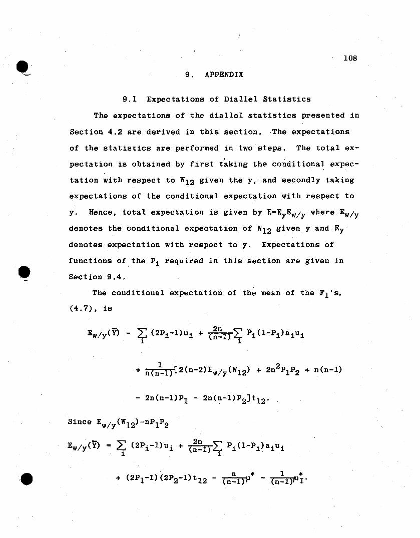
108
9. APPENDIX
9.1 Expectations of Diallel Statistics
The expectations of the diallel statistics presented in
Section 4.2 are derived in this section. The expectations
of the statistics are performed in two steps. The total ex-I
pectation is obtained by first taking the conditional expec-
tation with respect to Wl2 given the y,. and secondly taking
expectations of the conditional expectation With respect to
y. Hence, total expectation is given by E=EyEw/ y where Ew/ y
denotes the conditional expectation of Wl2 given y and Ey
denotes expectation with respect to y. Expectations of
functions of the Pi required in this section are given in
Section 9.4.
The conditional expectation of the mean of the FIls,
(4.7), is
Since Ew/y(W12)=nPIP2
Ew/y(Y) = ~ (2Pi -1)ui + (~~1)~ Pi (l-Pi )aiu i
n * I *(n-l)P - (n-1)ft I'
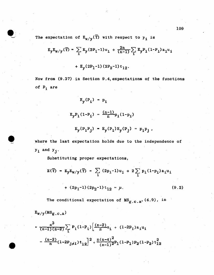
109
The expectation of Ew/y(Y) with respect to Yi is
Now from (9.37) in Section 9.4, expectations of the functions
of Pi are
where the last expectation holds due to the independence of
Yi and Yj'
Substituting proper expectations,
The conditional ex~ectation of MSg . c . a ' (4.9), is
Ew/y(MSg.c.a)
(9.2)
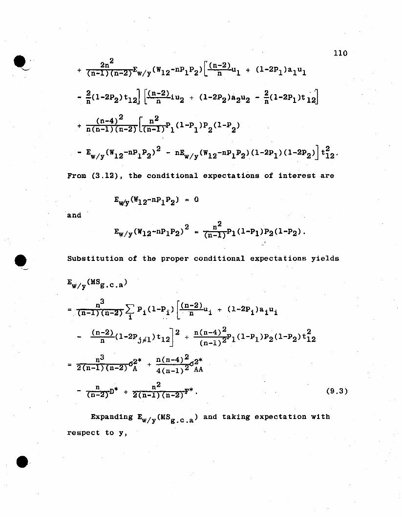
.'_. 110
- :(1-2P2)t12] [(n~2)iU2 + (1-2P2)a2u2 - *(1-2P1)ti~J
(n-4)2 [n2+ n(n-1)(n-2) (n-I)P1(1-P1 )P2 (1-P2 )
From (3.12), the conditional expectations of interest are
and
Substitution of the proper conditional expectations yields
EW/y(MSg.c.a)
n3
" [(n-2)='(n-l)(n-2)~Pl(1-Pi) 'n u i + (1-2Pi )a i u ii ..
(n-2) J2 n(n-4)2 2n (1-2Pj~1)t12 + (n_l)2P1(1-P1)P2(1-P2)t12
n3 2* + n(n-4)262*= 2(n-l)(n-2)6A 4(n-l)2 AA
n * n2- (n-2)D + 2(n-l)(n-2)F*. (9.3)
e,
Expanding ~/y(MSg.c.a) and taking expectation with
respect to y,
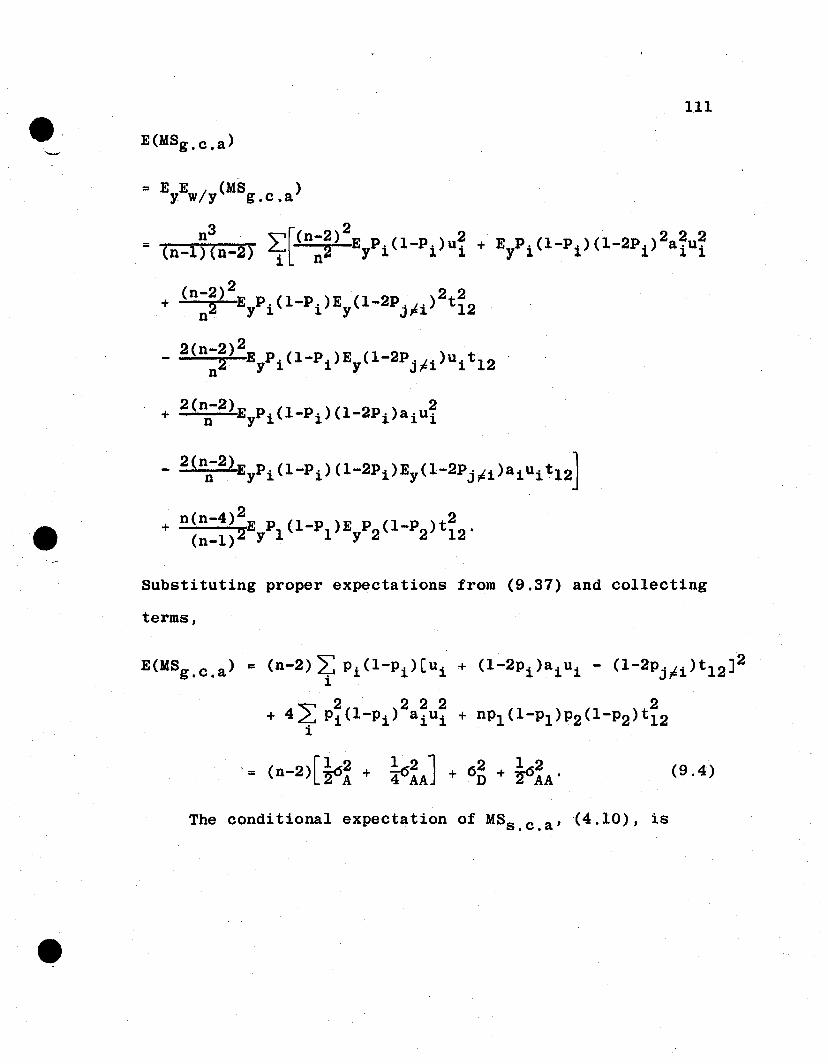
e·111
E(MSg . c . a )
= EyEw/y(MSg.c.a)
n3 ~r.(n-2)2 2 2 2 2= (n-l)(n-2) ~L n2 EyPi(l-Pi)ui + EyPi (1-Pi )(1-2P i ) aiui
(n-2)2 2 2+ n2 EyPi(1-Pi)Ey(1-2PjFi) t 12
2(n-2)2- n2 EyPi(1-Pi)Ey(1-2PjFi)uit12
Substituting proper expectations from (9.37) and collecting
terms,
[1 2 1 2 1 2 1 2= (n-2) ~A + i6AAJ + 6n + i6AA'
The conditional expectation of MSs . c . a ' -(4.10), is
(9.4)
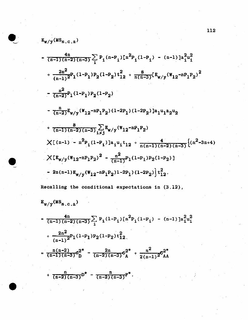
e·-",,~,/
112
+ Cn-i) (n~2) (n-3) i~Ew/y(w12-nPlP2 )
X[(n-l) - n2~i(1-Pi}Jaiuit12 + n(n-l)(:-2)(n-3) l(n2
-3n+4)
XC 2 n2Ew(y(W12-nPIP2) - (n_l)Pl(1-Pl)P2(1-P2)]
- 2n(n-l)Ew/Y(W12-nPlP2)l-2Pl)(1-2P2)Jt~2'
Recalling the conditional expectations in (3.12),
4n "" 2 2 2= (n-l)(n-2)(n-3)~ Pi(l-Pi)[n Pi(l-Pi ) - (n-l)]aiui
1.
2n2 2+ (n_l)2P1 (1-Pl)P2(1-P2)t12 ..
n(n-2) 2* 2n 62* n2 2*= (n-l)(n-3)6n - (n-2)(n-3) A + 2(n_l)26AA
n * n *+ (n-2)(n-3)D - (n-2)(n-3)F
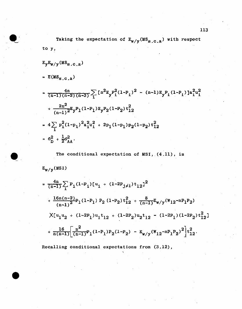
e.
113
Taking the expectation of Ew/y(MSs.c.a) with respect
to y,
= E(MSs . c •a )
= 4n "'" [n2E P2 (1_P )2 _ (n l)E P (1 P ) ]a2u2(n-l)(n-2)(n-3)~ y i i - . Y i - iii
2n2 2+ (n_l)2EyPl(1-Pl)EyP2(1-P2)t12
= 4L P~(1-P1)2a~u~ + 2Pl(1-Pl)P2(1-P2)t~2i
The conditional expectation of MSI,.(4.11), is
16n(n-2) 2 8+ 2 PI (I-PI) P2 (1-P2 ) t 12 + ( 1)Ew/y(W12-nPIP2)
(n-l) . n-
X[ul u2 + (1-2Pl )ul t 12 + (1-2P2 )u2 t 12 - (1-2Pl)(1-2P2)t~2]
Recalling conditional expectations from (3.12),
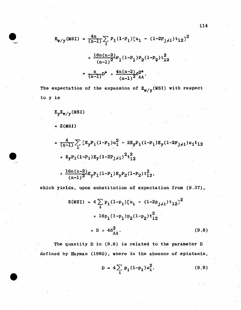
114
+ 16n(n-2)p (l-P )P (l-P )t2(n_l)2 1 1 2 2 12
== n n* + 4n(n-2) 62*(n-i) (n-1)2 AA'
The expectation of the expansion of Ew/y(MSI) with respect
to y is
= E(MSI)
which yields, upon substitution of expectation from (9.37),
E(MSI) = 44: Pi (l-Pi)[ui - (l-2Pj~i)t12]2J.
2+ 16Pl(l-P1)P2(l-P2)t12
2= D + 46AA . (9.8)
The quantity D in (9.8) is related. to the parameter D
defined by Hayman (1960)., where in the absence of epistasis,
•D = 4~ Pi(l-Pi )u~.
J.
(9.9)
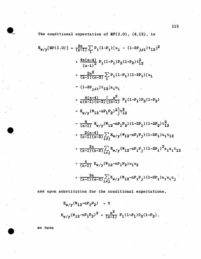
115
The conditional expectation of MP(I.O), (4.12),is
+ 4n(n-4) P (l-P )P (l-P )t2(n_l)2 1 1 2 2 12
+ (n-~)~n-2) ~ Pi (1-Pi)(1-2Pi) CUi
(1-2Pj~i)t12Jaiui
4(n-4) L n2+ n(n-l) (n-2) [(n-l) P1 (1-P1)P2 (1-P2)
- Ew/y(W12-nPIP2)2Jt~2
4 2- (n-l) Ew/y(W12-nPIP2)(1-2Pl)(1-2P2)t12
2(n-4»)1 ( (+ (n-l) (n-2)
ttjEw/ y W12-nPi Pj) 1~2Pi)uit12
+ ( 1~( 2)LE / (W12-np.p.)(1-2p.)2a.u.t12n- n- i~j w y 1 J 1 1 1
and upon substitution for the conditional expectations,
EW/y(W12-nPIPZ) = 0
Z n2Ew/y(W1Z-nPIPZ) = (n-l) P1 (1-P1)PZ(1-P2),
we have
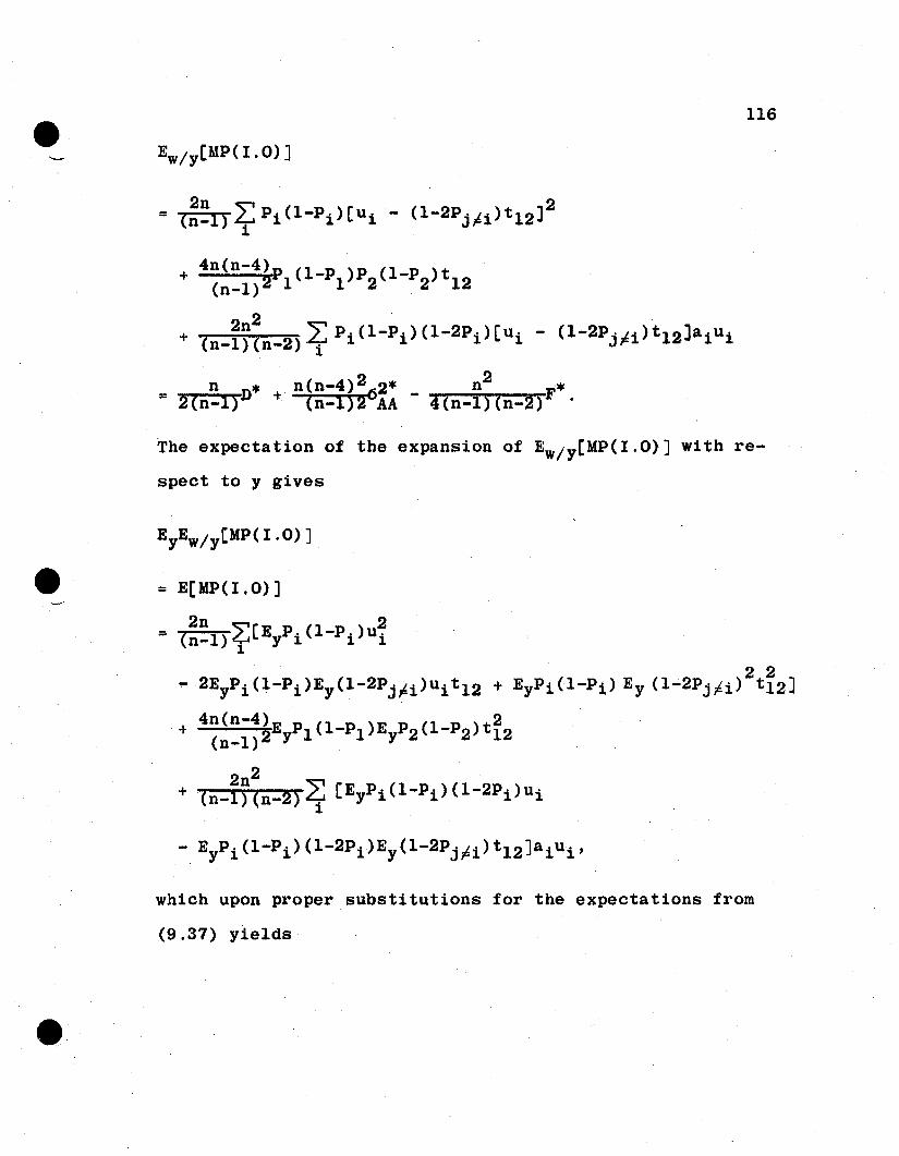
116
2n " . 2= (n_l)~Pi(l-Pi)[Ui - (1-2Pj /: i )t12 ]i
4n(n-4)+ (n_l)2Pl(1-Pl)P2(1-P2)t12
2n2 ~+ . ~Pi(1-Pi)(1-2Pi)[ui - (1-2PJ'1i)t12Jaiui(n-l)(n-2) i F
n * n(n-4)2 2* n2 *= 2(n-l)D + (n-l)26AA - 4(n-l) (n_2)F .
The expectation of the expansion of Ew/y(MP(I.O)] with re
spect to y gives
= E[MP( I.0)]
= (:~l)~[EyPi(l-Pi)U~1
which upon proper substitutions for the expectations from
(9.37) yields
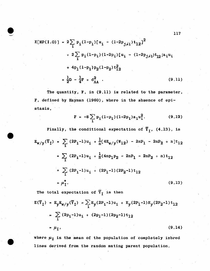
E[MP(LO) ]
117
= 2~ Pi(l-Pi)[ui - (1-2Pjpi)t12)2~
+ 2L Pi(l-Pi) (1...;2Pi)[ui - (1-2pjpi)t12 j a i u ii
+ 4Pl(1-Pl)P2(1-P2)tf2
112= 2D - 4F + 6AA
(9.11)
The quantity, F, in (9.11) is related to the parameter,
F', defined by Hayman (1960), where in the absence of epi-
stasis,
F = -84:Pi(1-Pi)(1-2Pi)aiu~.~
(9.12)
Finally, the conditional expectation of YI , (4.13), is
= ~ (2Pi -l)ui + ~(4nPIP2 - 2nPl - 2nP2 + n)t12~
*=PI'
The total expectation of YI is then
(9.13)
= 2: (2Pi-l)ui + (2Pl-l)(2P2-1)t12i
= PI' (9.14)
where PI is the mean of the population of completely inbred
lines derived from the random mating parent population.
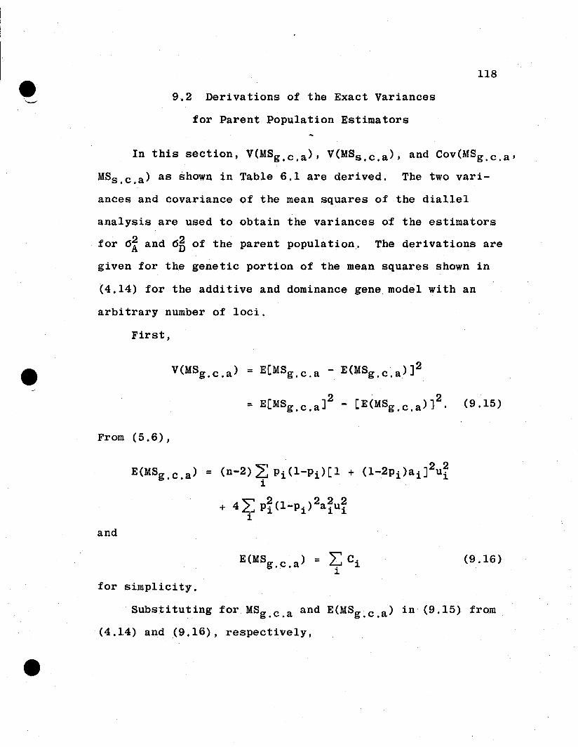
118
9.2 Derivations of the Exact Variances
for Parent Population Estimators
In this section, V(MSg . c . a ), V(MSs . c . a ), and Cov(MSg . c . a ,
MSs . c . a ) as shown in Table 6.1 are derived. The two vari-
ances and covariance of the mean squares of the dial leI
analysis are used to obtain the variances of the estimators
for cs~ and 6~ of the parent population.. The derivations are
given for the genetic portion of the mean squares shown in
(4.14) for the additive and dominance gene model with an
arbitrary number of loci.
First,
V(MSg . c . a ) = E[MSg . c . a - E(MSg . c . a)]2
2·· 2= E[MSg . c . a ] - [E(MSg . c . a )l. (9.15)
From (5.6),
E(MSg . c . a )
and
for simplicity.
= L: c.. 1.1.
(9.16)
Substituting for MSg . c . a and E(MSg . c .a ) in (9.15) from
(4.14) and (9.16), respectively,
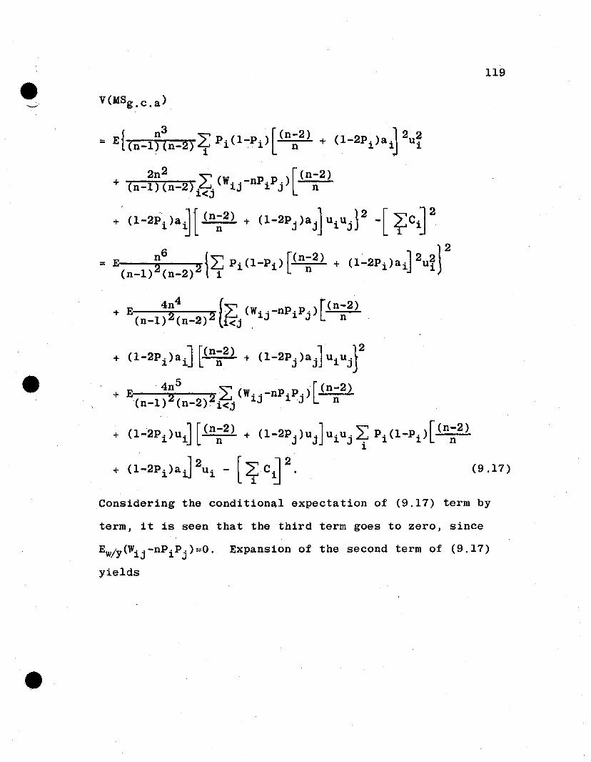
--.119
V(MSg • c . a )
· E! (n-l~~n-2) ~ Pi (I-Pi) [(n;2 l + (1-2Pilai] 2u~
2n2 ~ [(n-2)+ (n-l)(n-2)i~j(Wij-nPiPj) n
+ (1-2PilaJl (n;2 l + (1-2Pj }aj )ui u j }2 -[ f:CiY= E n
6 {L: p. (l-P·) [(n-2) + (1:"2P.)a.J 2u2i l. 2(n_1)2(n_2)2 I i 1 1 n 1 1 )
4n4 {~ [(n-2)+ E. . (w·· -nP .P . )
(n-1)2(n-2)2 .. <j .1J 1 J. n
+ (1-2Pi l aJ ~(n;2l + (1-2Pj la j ]ui u jf+ E 4n
5 2: (w .. -np.p.)r (n-2){n-1)2(n-2)2 i <j 1J 1J L n
+ (1"-2Pi )uJ [(n~2) + (1-2Pj )Uj ] UiUj ~ Pi (l-P i )[ (n~2)1
... (1-2P i )a i] 2Ui - [~cJ 2. (9.17)
Considering the conditional expectation of (9.17) term by
term,it is seen that the third term goes to zero, since
EW/y(Wij-nPiPj)~O. Expansion of the second term of (9.17)
yields
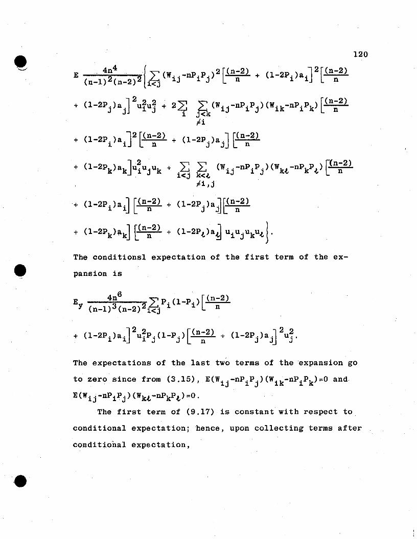
120
E . 4n4
.. .( ~ (W P P ) 2 f.(n-2) (1-2P.)a.J 2[(n-2)(n-l)2(n-2)2~. ij-n i j l n + 1 1 n
+ (1-2P.)a '12u?u~ + 2~ ~ (WiJ·-nPiPJ.) (Wik-nPiPk ) [(n-2)
J j 1 J i j<k n~i
+ (1-2Pi
)aiJ2 t(n~2) + (1-2Pj )a j ] t(n~2)
+ (1-2Pk)ak}.i~UjUk + i~ ~.(, (Wij-nPiPj)(Wkt-nPkP.(,)t(n~2)~i,j .
'+ (1-2P )aJ [(n-2) + (1-2P.)alL(n-2)i i n J ~[ n
The conditionsl expectation of the first term of the ex-
pans ion is
]2 2 [(n-2) U2 2+ (1-2P.) a . u . P . (l-P .) + (1-2P.) a. u ..
1 1 1 J J n J J J
The expectations of the last two terms of the 'expansion go
conditional expectation; hence, upon collecting terms after
conditional expectation,
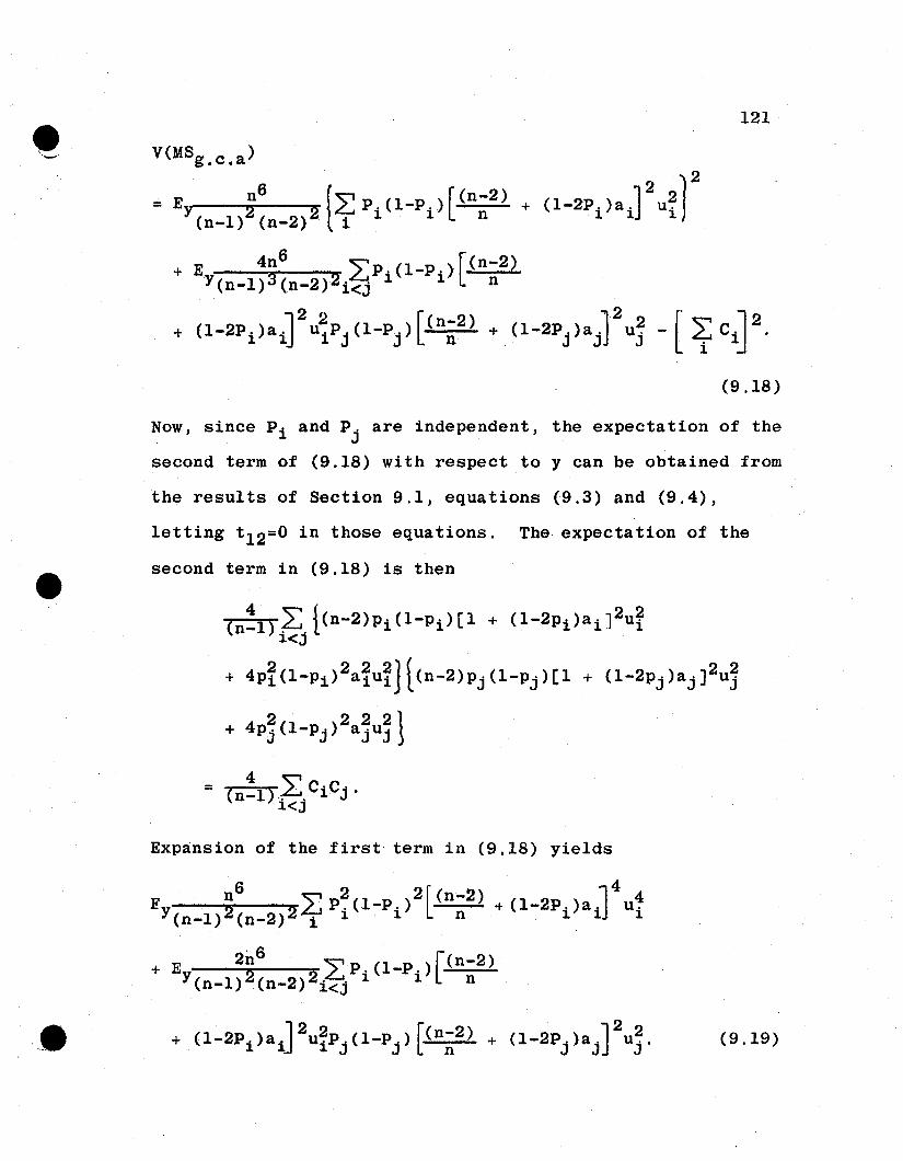
•'- 121
V(MSg •c •a )
= E n6
fL:p (l-P )[(n-2)Y(n-1)2(n~2)2liii n
+ E 4n6
LP.(1-p.)[(n-2)Y(n-l)3(n-2)2 i <j 1 1 n
J2 2 [(n-2) 122+ (1-2P.)a. u.P.(l-P.) + (1-2P.)a. u.
1 1 1 J. J. n . J J J
(9.18)
Now, since Pi and P. are independent, the expectation of the. J
second term of (9.18) with respect to y can be obtained from
the results of Section 9.1, equations (9.3) and (9.4),
letting t 12=O in those equations. The expectation of the
second term in (9.18) is then
(n~l)?=.{(n-2)Pi(1-Pi)[l + (1-2Pi)aiJ2u~1<J
+ 4P~(1-Pi)2a~u~Jt(n-2)Pj(1-Pj)[1 + (1-2Pj)aj]2u~
2 2 2 21+ 4pj (l-Pj) ajuj 5
Expansion of the first· term in (9.18) yields
(9.19)
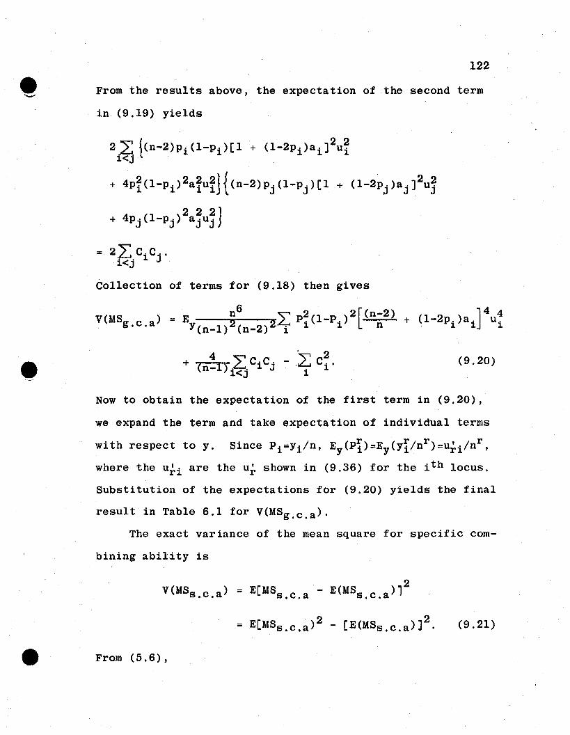
122
From the results above, the expectation of the second term
in (9.19) yields
")'1 222t<j l(n-2)Pi(1-Pi)[l + (1-2Pi)ai) ui
+ 4P~(1-Pi)2a~u~1{(n-2)Pj(1-Pj)[l + (1-2Pj)ajJ2u~
Collection of terms for (9.18) then gives
V. (MSg . c . a ) = E n6
~ P~(1_p.)2[(n-2) + (1-2P.)a.]4u~Y(n_l)2(n_2)2 i 1 1 n . 1 1 1
(9.20)
Now to obtain the expectation of the first term in (9.20),
we expand the term and take expectation of individual terms
with respect to y. Since Pi=Yi/n, Ey(pi)=Ey(yi/nr)=u~i/nr,
where the u~i are the u~ shown in (9.36) for the i th locus.
Substitution of the expectations for (9.20) yields the final
result in Table 6.1 for V(MSg . c . a )'
The exact variance of the mean square for specific com-
bining abil±ty is
V(MSs . c . a )
From (5.6),
2= E[MSs . c . a - E(MSs . c . a )l
(9.21)
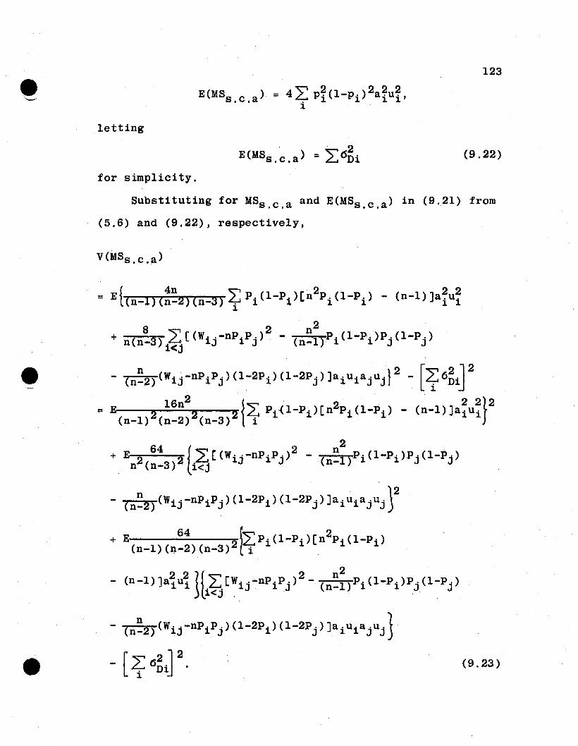
123
letting
(9.22)
for simplicity.
Substituting for MSs . c . a arid E(MSs . c . a ) in (9.21) from
(5.6) and (9.22), respectively,
= Ehn-l) (:~2) (n-3) ~ Pi (1-Pi )[n2
P i (I-Pi) - (n-l) ]a~u~
82 n2+ n(n-3) i~ [(Wij-nPiPj ) - (n-l)Pi (I-Pi)Pj (l-Pj )
e - (n~2)(Wij-nPiPj)(1-2Pi)(l-2Pj)]aiUiajujl2 - [~6~iJ2
l6n2 I ' 2· 2 2}2= E .22 2 2: Pi{l-Pi)[n Pi(l-Pi ) - (n-l)]aiui
(n-l) (n-2) (n-3) i
64 [" 2 n2
+ E 2L.,[(W' ·-np·p.) - (n_l)Pi(l-Pi)PJ.(I-PJ.)n (n-3)2 i<j 1J 1 J
n 12- (w· .-np·P.)(1-2p.)(1-2P.)]a.u.a.u.
(n-2) 1J 1 J 1 J 1 1 J J
2 2 1{"'" . 2 n2
- (n-l)]aiui Ji~[~ij-nPiPj) - (n_I)Pi(l-Pi)~j(l-Pj)
- (n~2)(Wij-nPiPj)(1-2Pi)(l-2Pj)]aiUiajUjJ
(9.23)
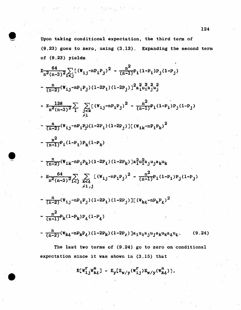
124
Upon taking conditional expectation, the third term of
(9.24)
The last two terms of (9.24) go to zero on conditional
expectation since it was shown in (3.15) that
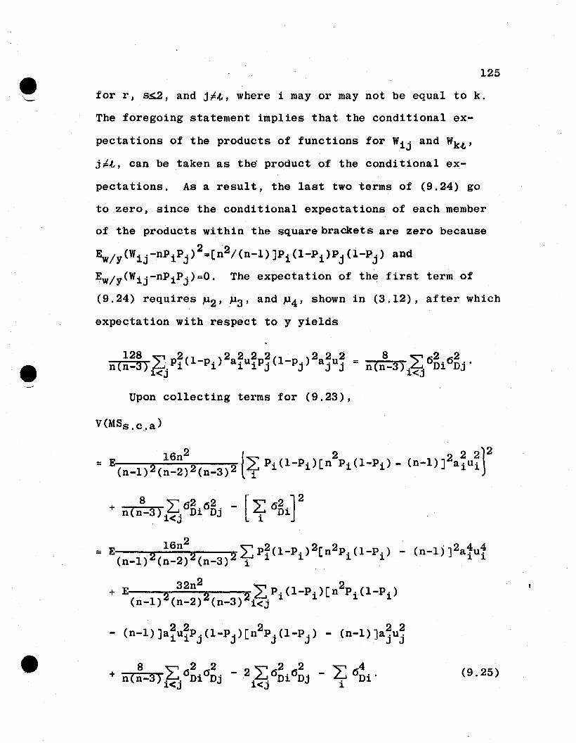
125
for r, s~, and j~~, where i mayor may not be equal to k.
The foregoing statement implies that the conditional ex-
pectations of the products of functions for Wij and Wk~'
j~t, can be taken as the product of the conditional ex-
pectations. As a result, the last two terms of (9.24) go
to zero, since the conditional expectations of each member
of the products within the square brackets are zero because
22·Ew/y(Wij-nPiPj) =[n /(n-l)]Pi(l-Pi)Pj(I-Pj ) and
Ew/y(Wij-nPiPj ) =0. The expectation of the first term of
(9.24) requires P2' P3' and P4' shown in (3.12), after which
expectation with respect to y yields
Upon collecting terms for (9.23),
V(MSs . c .• a )
_[L: 62.J 2. D1.1.
2= E 2 l6n 2 22: P~(l-Pi)2[n2Pi(I-Pi) - (n-l) ] 2atut
(n-l) (n-2) (n-3)i
32n2 ~ 2+ E. 2 22 ~ Pi (l-Pi)[n Pi (I-Pi)
(n-l) (n-2) (n-3) i<j
22· 2 2 2- (n-I)]a i ui Pj (I-Pj )[n Pj(l-Pj ) - (n-l)]ajuj
8,",22 ",2 2~4+ ( -3) ~6D"6D" -2~6D1."OD" - ~i 6D1."·n n i<j 1. J i<j J
(9.25)
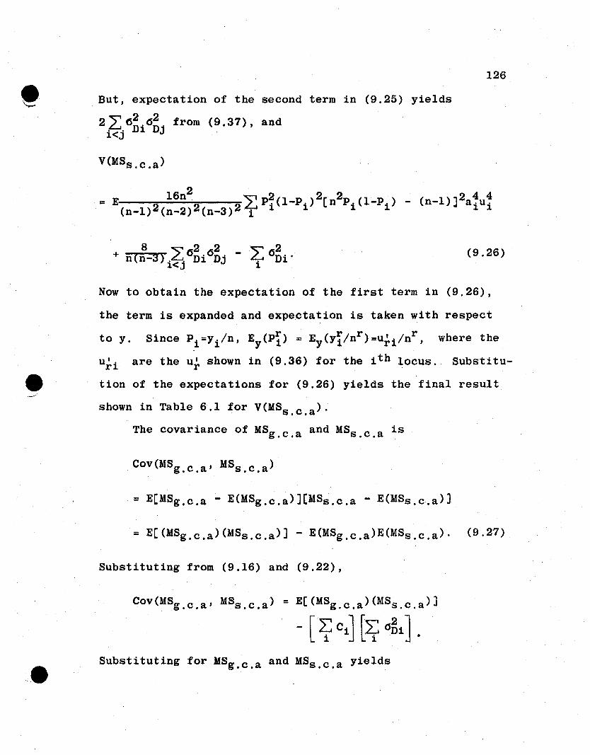
126
But, expectation of the second term in (9.25) yields
22; 6~i6~. from (9.37), andi<j J
V(MSs . c .a )
(9.26)
Now to obtain the expectation of the first term in (9.26),
the term is expanded and expectation is taken with respect
to y. Since Pi=yi!n, Ey(pi) = Ey(yi!nr)=u~1!nr, where the
u~i are the u~ shown in (9.36) for the i th locus. Substitu
tion of the expectations for (9.26) yields the final result
shown in Table 6.1 for V(MSs.c,a)'
The covariance of MSg . c . a and MSs.c,a is
COV(MSg . c . a ' MSs.c,a)
= E[MSg . c .a - E(MSg.c,a)][MSs,c.a - E(MSs.c,a)]
= E[(MSg.c.a)(MSs,c.a)] - E(MSg,c.a)E(MSs.c,a)' (9.27)
Substituting from (9.16) and (9.22),
Cov(MSg,c.a' MSs . c . a ) = E[(MSg.c,a)(MSs.c,a)]
- [zr Ci][~ 6~i]
Substituting for MSg . c . a and MSs . c . a yields
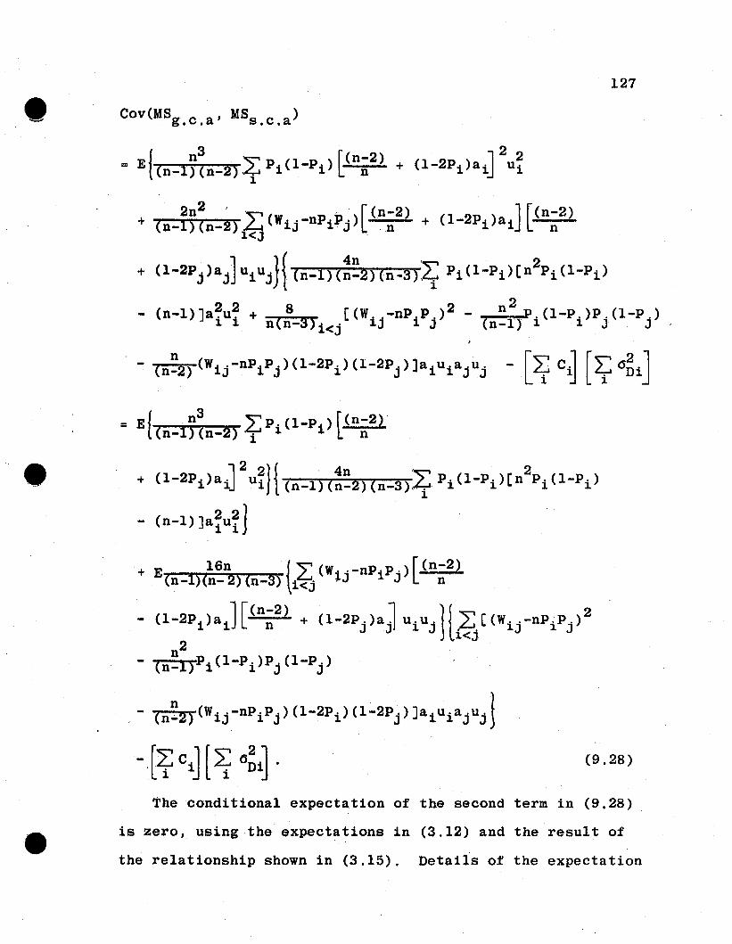
127
2n2 ' ."" .' [(n-2) ] [(n-2)+ (n-l)(n-2)~(Wij-nPiPj)n + (1-2Pi)ai n
1<J .
+ (1-2Pj )aj]ui uj}{ (n-l)(:~2)(n-3)~ Pi(1-Pi)[ n2Pi(1-Pi)
- (n-l)]a~U~ +8 [(wij
-nPi
Pj
)2 - n2
p .(1_P.)P.(1_P.)n(n-3) i<j (n-l) 1 1 J J
- (n~2) (Wij-nPiPj ) (1-2Pi ) (1-2Pj)]aiUiajUj - [2i c~ [~6~iJ
•= E[ n
3 ~ P (l-P ) [(n-2)(n-l) (n-2) ~ i i. n
+ E l6n{L:(W ._np.p.)[(n-2)(n-l)(n- 2) (n-3) i<j iJ 1 J n
- (l-2Pi)aiJ[(n~2) + (1-2PJ.)aJ uiu.]l L: [(w
iJ·-nPi P.)2
.J J li<j J
n2- (n-I)Pi(l-Pi)Pj(l-Pj ). ,
- (n~2) (Wij-nPiPj ) (1-2Pi ) (1-2Pj ) jaiUiajUj1(9.28)
The conditional expectation of the second term in (9.28)
is zero, using the expect~tions in (3.12) and the result of
the relationship shown in (3.15), Details of the expectation
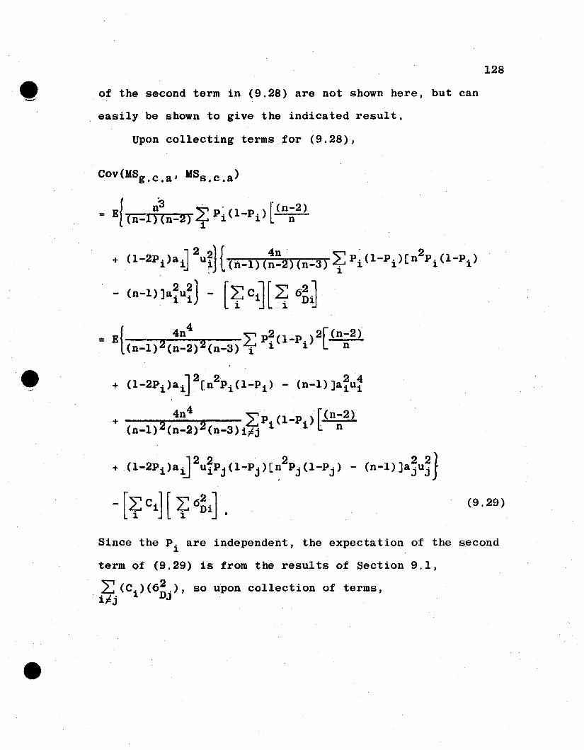
•128
of the second term in (9.28) are not shown here, but can
easily be shown to give the indicated result,
Upon collecting terms for (9.28),
Cov(MSg,c,a' MSs •c . a )
+ (1-2Pi )a i] 2u~J {(n-l) (:~2) (n-3) ~ Pi (1-P i )[n2
Pi (I-Pi)
(n-l) la~un - [~c~ [Lt /)~J
= E{ 4n4 L p 2 (1_P )2[(n-2)
(n-l)2(n-2)2(n-3), iii n
+ (1-2Pi)ai] 2[n2P i (I-Pi) - (n-l) ]a~u1
+ 4n4 L;p. (l-P.) [(n-2)
(n-l)2(n-2)2(n-3)i~j 1 1 n
(9.29)
Si,nce the Pi are independent, the expectation of the second
term of (9.29) is from the results of Section 9.1,
L: (C.)(62 .), so upon collection of terms,i~j 1 DJ
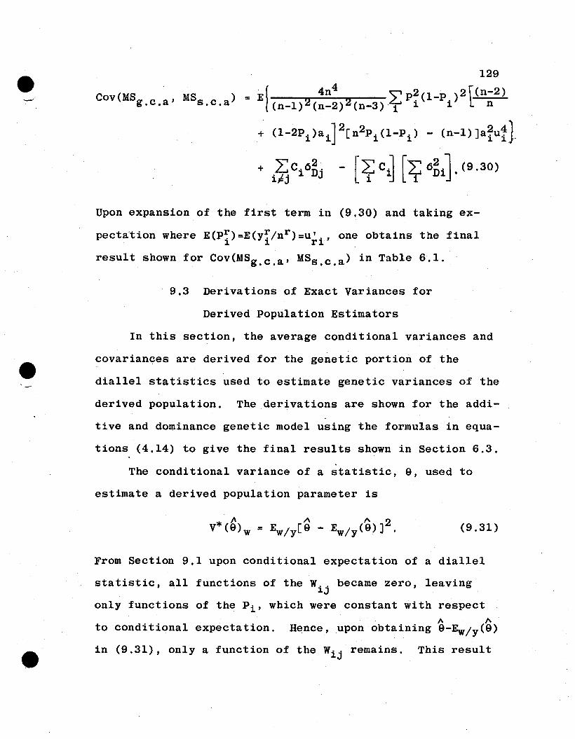
129
= E"! 4n4
P2 (1_P )2i(n-2)Cov(MSg . c •a ' MSs . c . a ) 2 2 ~(n-l) (n-2) (n-3)"i i i n
+ (1-2Pi)ai]2[n2Pi(1-Pi) - (n-l)Ja~ut}
Upon expansion of the first term in (9.30) and taking ex
pecta'tion where E(P::)=E(y::!nr)=u'., one obtains the final1 1 r1
result shown for COV(MSg . c . a , MSs •c . a ) in Table 6.1.
9.3 Derivations of Exact Variances for
Derived Population Estimators
In this section, the average conditional variances and
covariances are derived for the genetic portion of the
diallel statistics used to estimate genetic variances of the
derived population. The derivations are shown for the addi-
tive and dominance genetic model using the formulas in equa-
tions (4.14) to give the final results shown in Section 6.3.
The conditional variance of a statistic, 9, used to
estimate a derived population parameter is
(9.31)
From Section 9.1 upon conditional expectation of a diallel
statistic, all functions of the W.. became zero, leaving1J
only functions of the Pi' which were constant with respect
to conditional expectation. 1\ "Hence, upon obtaining 9-Ew!y(9)
in (9.31), only a function of the Wij " remains. This result
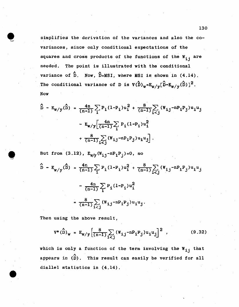
130
simplifies the derivation of the variances and also the co-
variances, since only conditional expectations of the
squares and cross products of the functions of the Wij are
needed. The point is illustrated with the conditional1\ 1\
variance of D. Now, D=MSI, where MSI is shown in (4.14).A 1\ 1\ 2
The conditional variance of D is V(D)w=Ew/y[D-Ew/y(D)] .
Now
Then using the above result,
(9.32)
which is only a function of the term invo~ving the Wij that1\
appears in (D). This result can easily be verified for all
diallel statistics in (4.14).
e--.131
Evaluating (9.32) gives
V*(~)w
= Ew/ y t(n~l){;j (Wij-nPiPj)UiUj] 2
= E / [ 64 L: (W .. -nPi P . )2u~u~w Y~n-l)2i<j 1J J J
From Section 3,
(9.33)
= E / (W .. -nP.P.)E / (w.k-nP.Pk )w y 1J 1 J W Y 1 1
:;: o.Also
=0.
Then the only remaining term to be evaluated in (9.33) is
v*(~)w = Ew/yr. 64 2.L.(Wij-nPiPj)2U~u~J 'L(n-l) 1<J
which yields from (3.12)
(9.34)
J'\which is the conditional variance of D. The average condi-
A
tional variance of D is
132J\
V*(D) =
and since the Pi are independent and from (9.37)
the average conditional variance of Dis
= (n~l) .2:.Di Dj ,l<J .
as shown in (6.2), where Di=4Pi(1-Pi)u~.1\
The conditional variance of F=2MSI-4MP(I.O), (5.7), is
upon substitution from (4.14),
since all cross products of Wij functions are zero on ex
pectation from Section 3. Now using (3.12),
1\V*(F)w
64n2 "V 2 2 2 2= 2 2 LJE / (Wi,-nP.P.) [U-2P.)a. + (1-2pJ.)aJ,] uiuJ'(n-l) (n-2) i<j w Y J 1 J 1 1
-133
1\which is the conditional variance of F. The average condi-
~ * ~ * ~tional variance of F is V (F) = Ey[V (F)wJ, whereupon sub-
stituting expectations from (9.37),
V*(F) = (n_l~tn_2)~jPi(1-Pi)U~[(n-2)Pj(1-Pj)(1-2Pj)2
+ 4p~(1-p.)2Ja~u~J J J J
+ (128 L:P1(1-P.i.)(l-2Pi)aiU~Pj(1-Pj)(1-2Pj)n-l)i<j
= 16 2:;D. [(n-2)~ + 62 ](n-l)(n-2)i~j 1 2 Aj Dj
which is shown in (6.2) where C5A2 .=2P.(1-P.)[1+ (1-2P.)a.J2u~,
J J J J J J
6~j=4P~(1-Pj)2a~u~, and Fj=-8Pj(1-Pj)(1-2Pj)ajU~.
The conditional variance of MSg . c . a , (4.14), is
V*(MS ) - E [MS - E (MS ) J2g.c.a - w/y g.c.a w/y g.c.a
J[(n-2)J J2+ (1-2P.)a. . + (1-2P.)a. u·u·.1 1 n J J 1 J (9.35)
134
The expectation of (9.35) was derived in Section 9.2 from
equation (9.17) and was shown to be
. . ~ 2 2 [(n-2) J2 2+ (1-2P.)a. u·P·(l-P.) + (1-2P·)a. u·,1 1 1 J J n J J. J
which is then the conditional variance of MSg . c . a ' The
average conditional variance of MSg •c .a is then
which was shown to be, from (9.18) in Section (9.2),
V*(MSg . c •a ) =
which is shown in (6,2),
The conditional variance of MSs . c . a ' (4.14) is
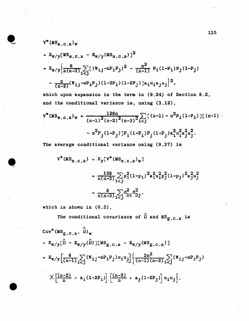
135
V*CMSs.c.a)w
= Ew/y[MSs.c.a - Ew/yCMSs.c.a)]2
[8 .', 2 n2
= Ew/ y n(n-3)i~[CWij-nPiPj) - (n-l) PiCl-Pi)PjCl-Pj)
- (n~2)CWij-nPiPj)Cl-2Pi)(1-2Pj)]aiUiajUjJ2,
which upon expansion is the term in (9.24) of Section 9.2,
and the conditional variance is, using (3.12),
* l28n "" 2V (MSs.c.a)w II 2 2 3 L..[Cn-l) - n PiCI-Pi)][Cn-l)(n-l) Cn-2) (n-3) i<j
2 2 2 2 2- n PjCI-Pj)]PiCI-Pi)PjCI-Pj)aiUiajuj.
The average conditional variance using C9.37) is
which is shown in C6.5).1\
The conditional covariance of D and MSg . c . a is
1\ 1\
= Ew/y[D - Ew/y(D)][MSg.c.a - Ew/y(MSg.c.a)]
= EW/Y[cn~l)i~ CWij-nPiPj)UiU~ {cn_~~~n_2)i~(Wij-nPiPj)
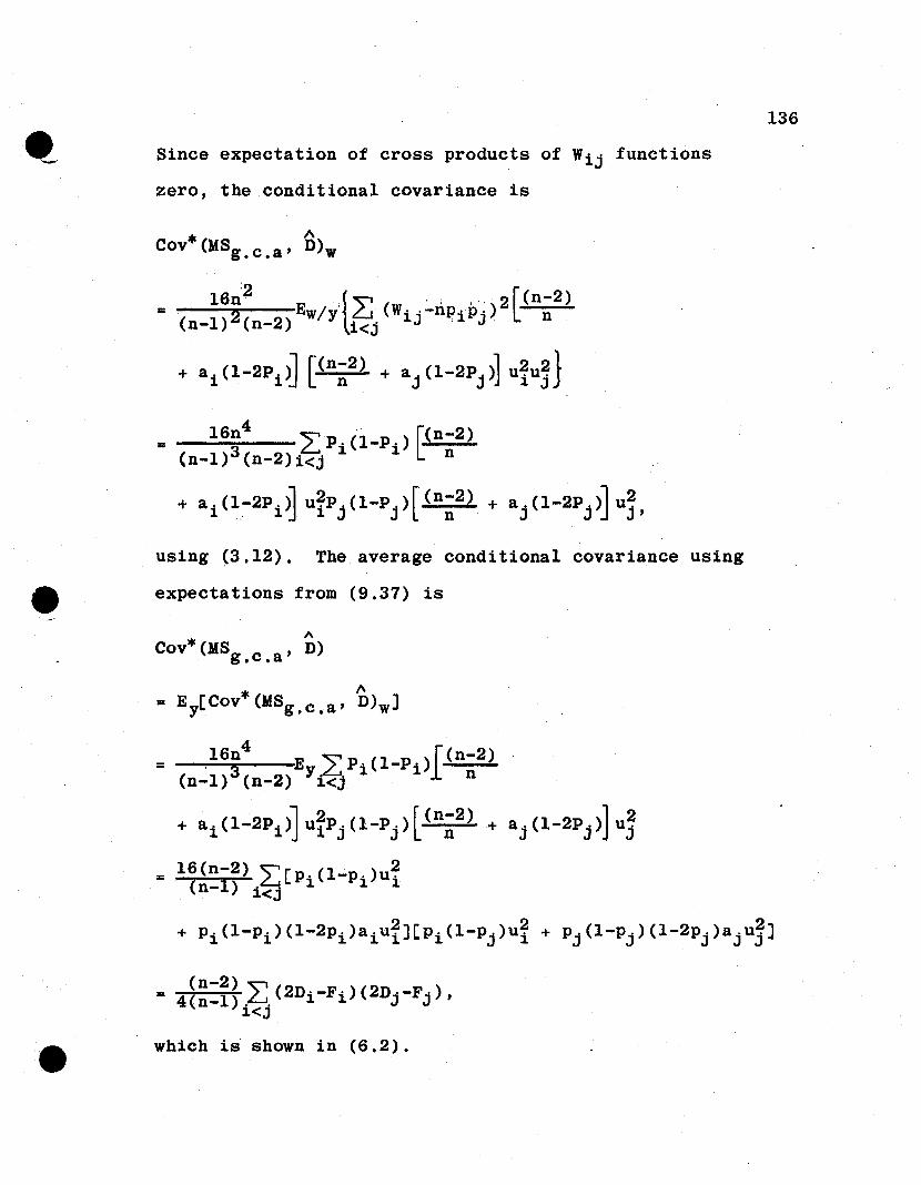
e--136
Since expectation of cross products of Wij functions
zero, the conditional covariance is
* ACov (MSg •c •a ' D)w
~ l6n4 L Pi (i-Pi) r(n-2)
(n-l)3(n-2)i<j L n
+ a i (1-2Pi )] U~Pj(1_Pj)[(n~2) + a, (1-2P,)1 u~J J J J'
using (3.12). The average conditional covariance using
expectations from (9.37) is
* 1\Cov (MSg •c .a ' D)
= .16n4
E >Pi(1-Pi)[(n-2)(n-l)3(n-2) y~ _ • n
+ a i (1-2Pi )] U~Pj (l-Pj ) [(n~2) + a j (1-2P j )] uj
= 16(n-2) ~[p,(l-p,)u~(n-l) i~ 1. 1. 1.- <J
+ p" (l-p" ) (1-2p" )a, u?] Cp. (l-p, )u? + PJ' (l-PJ") (1-2PJ' )aJ.uJ~]1. 1. 1. 1. 1. 1. J 1.
which is shown in (6.2).
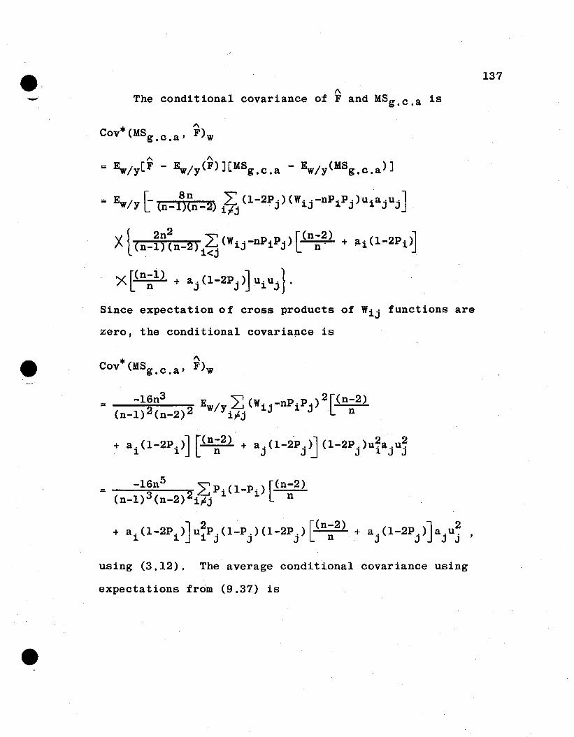
e· 1\The conditional covariance of F and MSg . c •a is
137
Since expectation of cross products of Wij functions are
zero, the conditional covariance is
= -16n3 E ~ (W .. _np.p.)2[(n-2)(n-l)2(n-2)2 W/Yipj 1J 1 J n
+ a. (1-2P.)J [(n-2) + a. (1-2P.)1 (1-2P. )u~a .u~1 1 n J J J J 1 J J
using (3.12). The average conditional covariance using
expectations from (9.37) is
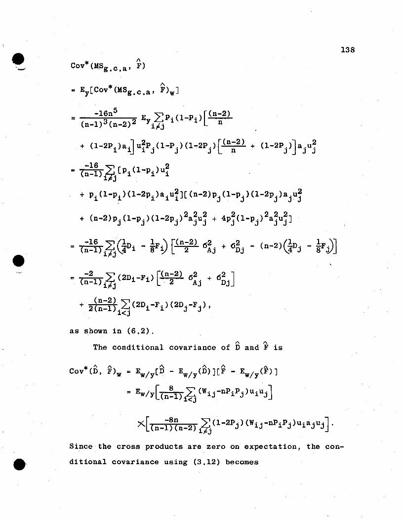
13S
* ACOV (MSg •c •a ' F)
J 2 ( ) ( [(n-2) ] 2+ (1-2P.)a i uiP. I-P. 1-2P.) + (1-2P.) a.u.1 J J J . n J J J
-16 ~ 2= (n-l) [Pi(l-Pi)uii j
+ Pi(1-Pi)(1-2Pi)aiu~J[(n-2)p.(1-P.)(1-2P.)a.u~1· J J J JJ
= -16 ~ (.lD. _ I F .\ [(n-2) 62 62 _ (n-2) (!-D. - slFJ.\l(n-l)~.~4 1 8 Y 2 Aj + Dj ~4 J VJ1FJ
as shown in (6.2).A A
The conditional covariance of D and F is
* h A ~ ~ A ACov (D, F)w = Ew/y[D - Ew/y(D)][F - Ew/y(F)]
= EW/Y[(n~l)i~ (Wij-nPiPj)UiUj]
Since the cross products are zero on expectation, the con-
ditional covariance using (3.12) becomes

"'~
139
The average conditional covariance is, using (9.37),
*'" 1\ *" "-COV (D, F) ~ Ey[Cov (D, F)w J
• (~~~)i~Pi(1-Pi)U~Pj(1-Pj)(1-2Pj)ajU~
= (n~l) i~DiF j'
as shown in (6.2).1\
The conditional covariance of MSs . c . a and F is
- n (W .. -nP.P.)(1-2P.)(1-2P.)a.u.a,u'J(n-2) 1J 1 J 1 J 1 1 J J
Since the expectations of cross products are zero, the
conditional covariance is
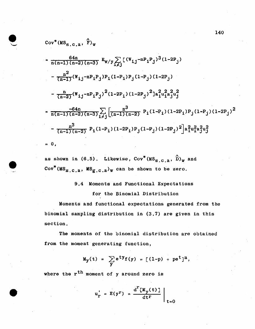
140
-64n 'C""l r. n3 . 2= n(n-1)(n-2)(n-3)i~jL(n-l)(n-2) Pi(l-Pi)(l-2Pi)Pj(l-Pj)(l-2Pj)
- (n-l)~n-2) Pi(l-Pi)(l-2Pi)Pj(l-Pj)(1-2Pj)2Ja~u~ajuj
= 0,
as shown in (6.5). Likewise, COV*(MSs . c . a ' D)w and
*Cov (MSs . c •a , MSg.c.a)w can be shown to be zero.
9.4 Moments and Functional Expectations
for the Binomial Distribution
Moments and functional expectations generated from the
binomial sampling distribution in (3.7) are given in this
section.
The moments of the binomial distribution are obtained
from the moment generating function,
t=o
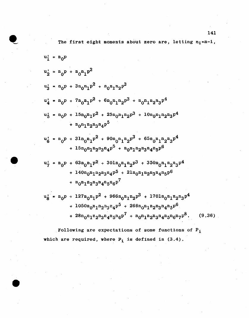
141
The first eight moments about zero are, letting ni=n-i,
u' nop 2= + nOnl P'2
u' 2 33 = nop + 3nOnl P + nOnl n2P
u' nop 7nOnlP2 + 6nOnln2P3 + 4
4 = + nOnl n2n3P
Us = nop + 15nonl P2 + 25nonln2P3 + lOnOnln2n3 P4
5+ nOnln2n3n4P
234+ 31nonlP + 90nOnln2P + 65nonln2n3P
+ 15nonln2n3n4p5 + nOnln2n3n4n5P6
ui = nop + 63nonlP2 + 301non1n2P3 + 350nOnln2n3P4
+ 140nOnln2n3n4P5 + 21nonln2n3n4n5P67
+ nOnln2n3n4n5n6P
Us' = nop + 127nonl P2 + 966nonl n2P3 + 1701nonln2n3P4
+ l050nOnln2n3n4P5 + 266nonln2n3n4n5P6
'+ 28nonln2n3n4n5n6P7 + nOnln2n3n4n5n6n7P8. (9.36)
Following are expectations of some functions of Pi
which are required, where Pi is defined in (3.4).
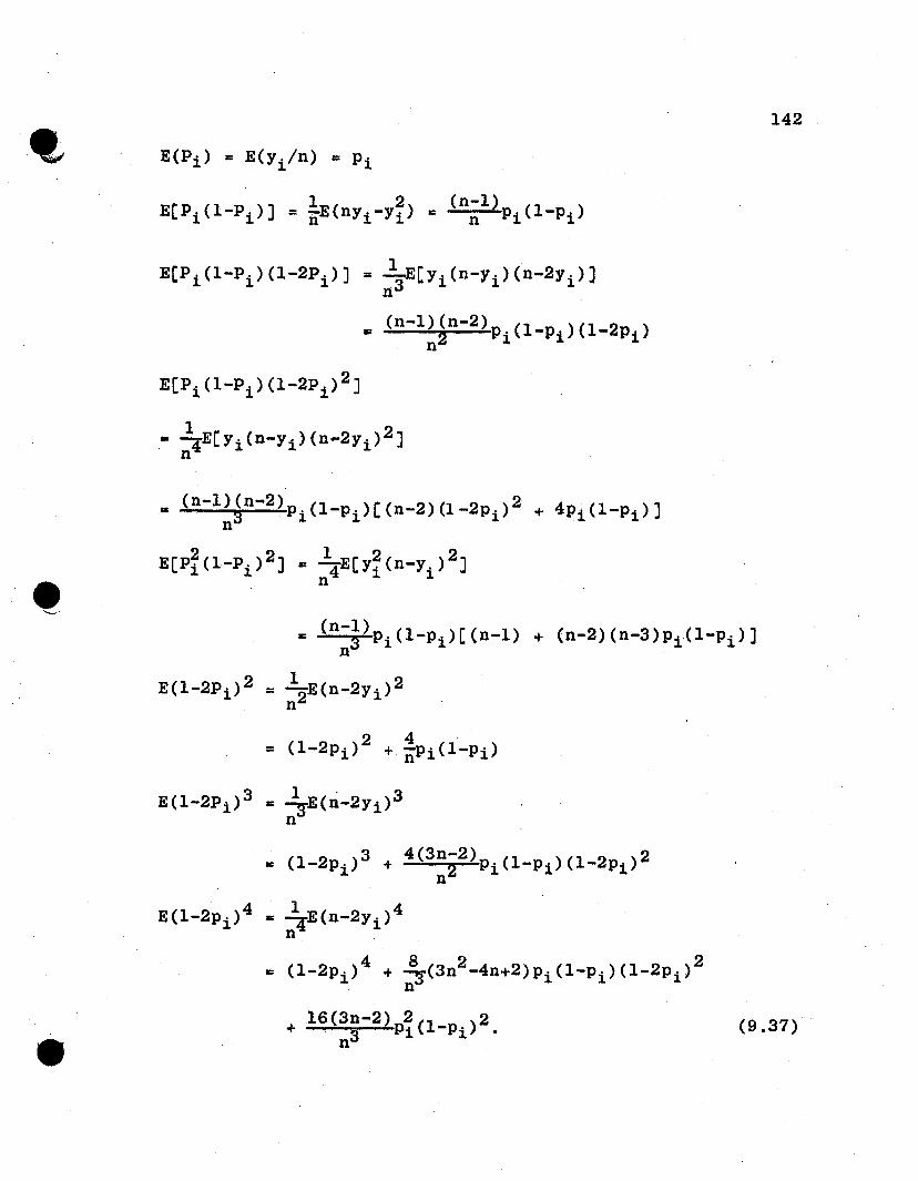
142
E(Pi) = E(Yi/n ) = Pi
1 2 (n-l)E[Pi (I-Pi )] = nE(nYi-Yi) ~ n Pi(I-Pi)
1 .= --E[Yi(n-Yi) (n-2Yi)]
ti3
~ (n-l)(n-2)p.(1_P.)(1_2Pi)21.1.n
• (n-l)(n-2)p.(I-p.)[(n-2)(1_2Pi)2 + 4Pi(I-Pi)]n3 . 1. 1.
E[P~(1-Pi)2] = ~E[y~(n-Yi)2]n
• (n-5)Pi(I-Pi)[(n-l) + (n-2)(n-3)Pi(1-Pi)]n
E(I-2Pi)2 = 12E (n-2Y i)2n
(9.37)
![Bayesian Analysis of Power Function Distribution Using ... · likelihood, moments and percentile estimators. Zaka and Akhter [43] derived the Bayes estimators using different loss](https://img.pdfslide.us/doc/110x75/5f0d88ca7e708231d43ad61f/bayesian-analysis-of-power-function-distribution-using-likelihood-moments-and.jpg)