LA-7534-MS

,.,,1

InformalReport

C3ClC-l 4 R’EPORT COLLECTION

REPRODUCTIONCOPY

Analysis of Laser Fusion Targets

Using Monochromatic X-Ray Microradiographs

(ls!!ikLOSALAMOS SCIENTIFIC LABORATORYPostOfficeBox 1663 LosAlamos.New Mexico87545

An Affirmative Action/Equal Opportunity Empbya

This report was prepared u an account of work sponwredby the United Stale. G.a.rrnm.nt. Neither the UnJl#d slut..nor the Unllod States Depuiment of Enersy, nor my of Ihclr9mP10Y..h nor any O( their c.ntm.tc.n. .ub.ontmctc.n. .rllwla employees. makes ●nY warranty, ●xprem or Impllal, orasaimes anY I.uI 11.blllly or rrapondbllily Ior Uw ●ccuracy,.ompletenem. ?t uiefulnen of ●ny In fommtlon, 8Pp.mtus.product, or Process dlccloicd. or t*PWWntI Ihnt lb UW WOUhinot In fIinS. PItV.t,lY owned rlshts.

UNITCD 8TATCS

DEPARTMENT OF CNCR~VCONTRACT w-7408 -8N0. SS

.

.

LA-7534-MSInformalReport

UC-21Issued:October 1978

Analysis of Laser Fusion Targets

Using Monochromatic X-Ray

R. L.WhitmanR. H. DayR. P. KrugerD. M. Stupin

r“

Microradiographs

;

ANALYSIS OF LASER FUSION TARGETS

USING MONOCHROMATIC X-RAY MICRORADIOGRAPHS

by

R. L. Whitman, R. H. Day, R. P. Kruger, and D. M. Stupin

ABSTRACT

A new contact microradiographic system for analyzinglaser fusion targets with two-dimensional modeling and image-analysis techniques is described. This system, which uses amonochromatic x-ray source and Kodak High-Resolution Plateemulsion, is sensitive to spherical wall-thickness variations(eccentricities) as small as t 200 A in hollow shells with amean wall thickness of 1 pm. Measurements of wall thicknessand of local and spherical wall-thickness variations by radio-graphic techniques, using two-dimensional video, digital imageanalysis, and optical interferometry, are compared. In addition,three digitizing systems are compared for converting the radio-graphic data to digital form.

I. INTRODUCTION

Theoretical calculations of laser-driven implosions predict that uniform,

symmetric shells are required for successful laser fusion targets. To date, the

most common target contains the fusible gas within a thin-walled spherical glass*

shell. The usable shells are typically 100 ~m in diameter with l-pm-thick

walls and have wall-thickness variations no larger than t 300 A. Optical inter-

ferometric techniques are adequate to measure wall-thickness uniformity to

+ 500 A and possibly to + 300 A.1,2 However, target designs are becoming more

complicated, some of them requiring optically opaque, multilayered materials.

Therefore, highly symmetric opaque shells will be required, and methods must be

*Several trademarks have been registered for this generic class of target: KMS‘Fusion, Inc., Microshell, as well as Errunersonand Cumnings, Inc., Glass Micro-balloon, and Eccosphere.

1

developed to characterize them. X-ray microradiography has been suggested as an

appropriate characterization technique. 3

We will describe a contact microradiographic system comprising monochro-

matic x-ray radiation, Kodak High-Resolution Plate (HRP) emulsion, a two-

dimensional analytic model, and digital image analysis techniques to inspect

opaque shells used as laser fusion targets. Monochromatic x rays from a modi-

fied Henke x-ray tube illuminate the hollow shells, and the images of the shells

are recorded on HRP emulsion (Section II). These microradiographs are digitized

into optical density values , and by a sectoring algorithm the digitized image of

the hollow shell is partitioned into many equal sectors. Differences in average

optical density of opposing sectors are averaged and converted, to eccentricity

(sphericity) using the results of computer-generated curves from two-dimensional

hollow shell models (Sections III and IV). A statistical outlier test is also

performed to detect local defects more than two standard deviations from the

average sector densities in the hollow shells (Section IV). For convenience we

divide the experimentally observed defects into three classes and demonstrate

the sensitivity of our method in detecting each class (Sections IV and V). Its

sensitivity will be compared to the sensitivities of optical interferometry mea-

surements and radiographic measurements using analog video analysis techniques

(Section VI). In addition, three image digitizing systems are compared for

scanning the microradiographs (Section VII).

II. RADIOGRAPHICSYSTEM

To achieve the highest sensitivity to defects, the three

of the radiographic system must be optimized. They are (1) the

(2) the microsphere film-imaging system, and (3) the radiograph

each of which is discussed in detail below.

A. X-ray Source

major components

x-ray source,

readout system,

Two x-ray sources have been used at the Los Alamos Scientific Laboratory

(LASL) to radiograph laser fusion targets. The primary source used for exposures

with ultrasoft x rays (c 1 keV) is a modified Henke x-ray tube with interchange-

able anodes to allow us to excite various ultrasoft x-ray lines from 0.109 to

1.5 keV.4 This flexibility permits us to choose the x-ray energy that will pro-

duce the maximum contrast in the film image.5 The anode potential is restricted

to about twice the characteristic line energy to suppress high-energy bremsstrah-

lung. By filtering the x-ray beam, we can restrict the spectral contaminants to

2

.

.

.

>

.

less than 10% of the total fluence. To achieve maximum fluence at low anode-

cathode voltages, we have replaced the tungsten filament with thorium-oxide

(ThO)-coated Ir ribbons placed directly in front of the anode. The high emis-

sivity of these filaments at low temperatures (1600-2000°C) keeps the surface

contamination to negligible levels, as verified by crystal spectroscopy. We are

using the CuLa line at 930 eV to radiograph l-pm-thick glass shells, and are de-

veloping a high-intensity, ultrasoft x-ray source using a modified Pierce elec-

tron gun to replace the Henke source.

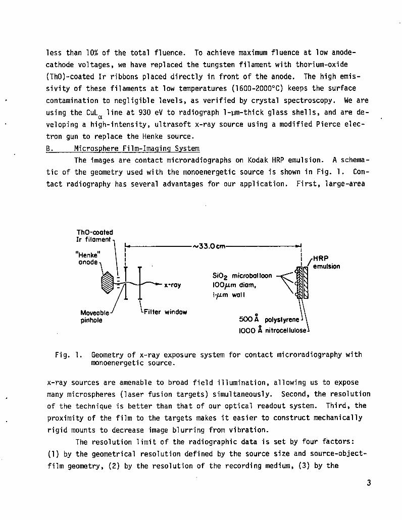
B. Microsphere Film-Imaging System

The images are contact microradiographs on Kodak HRP emulsion. A schema-

tic of the geometry used with the monoenergetic source is shown in Fig. 1. Con-

tact radiography has several advantages for our application. First, large-area

ThO-tootedIr filoment

1 ~wss.ocm~“Henke”

1-

iI

ionode HRP

~TI ![ emulsion

Si02 microbdloon

V .–

x-roy 100~m diem,l-~m wolI x[~

\Moveoble] ~Filterwindowpinhole 500~ polystyrene\\

iOOO A nitrocellulose~

Fig. 1. Geometry of x-ray exposure system for contact microradiography withmonoenergetic source.

x-ray sources are amenable to broad field illumination, allowing us to expose

many microsphere (laser fusion targets) simultaneously. Second, the resolution

of the technique is better than that of our optical readout system. Third, the

proximity of the film to the targets makes it easier to construct mechanically

rigid mounts to decrease image blurring from vibration.

The resolution limit of the radiographic data is set by four factors:

(1) by the geometrical resolution defined by the source size and source-object-

film geometry, (2) by the resolution of the recording medium, (3) by the

3

resolution of the image readout system, and (4) by the resolution due to x-ray

diffraction in the object. For maximum speed and sensitivity of the system, the

first three of these limits of resolution should be comparable in size while en-

suring that image blurring due to x-ray diffraction is negligible. These three

resolution limits are: geometric resolution, 0.5 pm; resolution of Kodak HRP,

0.5 pm; and picture-element (pixel)size of the image readout system (a Photometric

Data Systems [PDS] Model 1050 Scanning Densitometer), 2.0 pm. These estimates

are higher than the x-ray diffraction limit of resolution, 0.06 pm, for the geom-

etry and monochromatic x-ray energy used here.6 Therefore, the limit of resolu-

tion of the present system is defined by the 2-pm pixel size of the image-scanning

system. In comparison, the best optical microscopes would have been an almost

ten times higher resolution and would be used if such fine detail were important

for future applications.

Object mounting for contact microradiography imposes the additional con-

straints: (1) the microsphere support structure should be vacuum-compatible and

should not absorb the exposing x-ray radiation, and (2) the microsphere should

be removable for use or reorientation.7 A technique that would meet both criteria

simultaneously has not yet been identified, although several are being investi-

gated. We are presently using a method in which the microsphere are glued by a

500-A polystyrene film to a 1OOO-A nitrocellulose layer. The transparent backing

allows us to radiograph the image and to inspect the microsphere interferometri-

cally in the same orientation.

The sensitivity of the HRP emulsion was measured for the x-ray energies

of interest, and the resultant optical densities versus exposure levels, i.e.,

H-D curves, are shown in Fig. 2. The specular density was measured with a PDS

scanning microdensitometer.

c. Image Inspection System

The images were read with the PDS densitometer using a2-by 2-pm aperture

stepped in l-pm increments in both the x- and y-directions over a raster pattern

sufficient to cover the image. The noise in the system is due to both the film

grain noise of the emulsion and the photomultiplier noise of the densitometer

(Fig. 3). These noises combine to generate an effective single-point noi:ea aD.

The value of OD was found empirically to be well described by a power law ‘ for

optical densities above 0.1.

.

.

.

‘D = 0.062 D0”8 .

4

(1)

4.0 ‘ I I i I I 1 I I I I I I 1 I I i

3.6 - 0 AI K= Rodiation

~ Cu La Radiation3.2 - a 4-kV Bremsstrohlung on W

2.6 -

g

~ 2“4 -

3g 2.0-0&

31.6 -

&1.2 -

0.8 -

04 -

u

102 103 10’Exposure (photons/#m2)

Fig. 2. Total exposure as a function of optical density for HRP emulsion.

Lo- 1 I I I I I I 1[ 1 i

.

Fig. 3.

Opticol Density

MS system noise, OD, as a function of HRp emulsion density.

5

The flatness of the background density is better than 1% over most of the field,

however, there is an additional time-dependent base level shift of about 0.03

optical density units per minute, which necessitates “rezeroing” the densitometer

between images. This makes measurements of very low densities less accurate.

III. TWO-DIMENSIONALMODEL

We simulated a two-dimensional x-ray radiographic image of an 80-pm-diam

glass microsphere with a l-pm-thick wall. This simulation is an extension of a

one-dimensional model discussed previously and is described in Appendix A. The

simulated images were used as standards to determine the baseline sensitivity of

the sphere mensuration algorithm. The model includes as input: the microsphere

diameter, wall thickness, wall composition, source size, photon energy, total ex-

posure, the source-to-film distance, microsphere-to-film distance, the character-

istic curve of the film, and the film-recording system noise. Programmed eccen-

tricities of the inner and outer surfaces of the microsphere were introduced to

study the sensitivity of the proposed computer eccentricity measurements.

A 100-pm-diam microsphere with a l-~m-thick wall as scanned by the PDS

microdensitometer and displayed on a COMTAL digital video is shown in Fig. 4a,

and may be compared to a simulated 80-pm-diam microsphere of the same wall thick-

ness, with noise, OD, added, as shown in Fig. 4b. Similarly modeled images are

used to calibrate our sensitivity to detecting each of three classes of defects,

which we discuss in Section IV.

IV. TWO-DIMENSIONALANALYSISFOR THREE CLASSES OF IMAGE DEFECTS

We have experimentally observed three classes of defects in thin-walled

microsphere. To analyze their severity, we have devised a two-dimensional analy-

sis technique to detect the three classes of defects. Type-I defects are modeled

as an eccentricity of the spherical surfaces defining the inner and outer walls

of the microsphere; Type-II defects are modeled as a nonsphericity of one or both

of these walls; and Type-III defects are associated with small-scale nonuniformities

in the wall composition or thickness (e.g., lumps and holes). We will first out-

line a general algorithm that is sensitive to detecting Type-I and some Type-II

defects; and second we will outline a general algorithm that is sensitive to small

Type-II and Type-III defects.

.

.

.

6

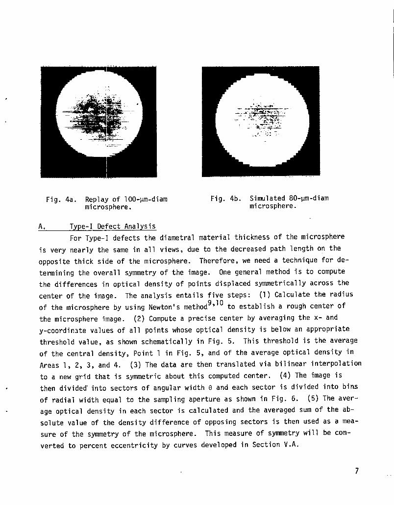
Fig. 4a. Replay of 100-pm-diammicrosphere.

Fig. 4b. Simulated 80-um-diammicrosphere.

A, Type-I Defect Analysis

For Type-I defects the diametral material thickness of the microsphere

is very nearly the same in all views, due to the decreased path length on the

opposite thick side of the microsphere. Therefore, we need a technique for de-

termining the overall symmetry of the image. One general method is to compute

the differences in optical density of points displaced symmetrically across the

center of the image. The analysis entails five steps: (1) Calculate the radius

of the microsphere by using Newton’s method9,10 to establish a rough center of

the microsphere image. (2) Compute a precise center by averaging the x- and

y-coordinate values of all points whose optical density is below an appropriate

threshold value, as shown schematically in Fig. 5. This threshold is the average

of the central density, Point 1 in Fig. 5, and of the average optical density in

Areas 1, 2, 3, and 4. (3) The data are then translated via bilinear interpolation

to a new grid that is symmetric about this computed center. (4) The image is

then divided into sectors of angular width 0 and each sector is divided into bins

of radial width equal to the sampling aperture as shown in Fig. 6. (5) The aver-

age optical density in each sector is calculated and the averaged sum of the ab-

solute value of the density difference of opposing sectors is then used as a mea-

sure of the symmetry of the microsphere. This measure of symmetry will be con-

verted to percent eccentricity by curves developed in Section V.A.

7 -._

I I II Film

I I background ~

IImoge Cross

Section[level, ,

—— —---- .—— ———---—- —- —----= A

.- Filmfog L Thresholdg level~a

●1

Distance(~m )

Fig. 5. Diagram of microsphere radio-graph and cross section.

B. Type-II and -III Defect Analyses

Fig. 6. Sectored microsphere. Formaximum sensitivity the cal-culation considers an annulusfrom 40 to 80% of the micro-sphere radius enclosed bv the.

% axradii.

For Type-II and Type-III defects we can detect the nonuniformity as a de-

viation of the observed optical density from the average appropriate for each

case. One method for detecting a Type-II defect requires taking at least three

identical radiographs of the microsphere in independent orientations and comparing

the mean densities in the centers of the images.

For a Type-III defect, we scan the image surface and determine whether

statistically significant anomalies occur. We have defined a general technique

for doing this, which employs a statistical T-test.ll This analysis uses Steps 1

through 4 described above for detecting Type-I defects plus six additional steps:

(1) Define an area of approximately L x L pmz (where L>l pm) and average the

optical densities in that area (Fig. 6). The usual area size is several sector

widths by several bin heights (e.g., in Section V.B, L x 7 pm). (2) The L x L

area is stepped around the microsphere at a constant radius by sector increments,

resulting in overlapping L x L adjacent areas, e.g., 2.5 degrees. (3) An average

8

.

.

optical density and uncertainty in the optical density is computed for all over-

lapping L x L areas at that radius. (4) The average density is subtracted from

all densities for the L x L areas and divided by the standard deviation in optical

density. This results in a signal-to-noise (s/N) ratio S. (5) If this ratios

S, is above 2, a “warning” output is given. If above 3, a “bad” output is given.

These limits can be changed. In addition, the location of the defect, the mean

wall thickness in micrometers, and the mean defect thickness in micrometers are

calculated. (The procedure for calculating the thicknesses is shown in Appendix

Be) (6) Steps 2 through 5 are repeated for all L x L areas at an increased radius

of one bin width (usually 1 pm). The computation is usually repeated for radii

from 10 to 95% of the computed radius. The output gives a footprint of the small

Type-II and Type-III defects.

Taking this technique one step further, it will be possible to group the

overlapping”L x L adjacent defective areas together by a feature-clustering method

to make a composite image of the position, size, shape, and mass of each defect.

u. SENSITIVITY OF TWO-DIMENSIONAL ANALYSIS TECHNIQUES

We next consider the sensitivity of two-dimensional analysis of x-ray

microradiographs in detecting the types of defects defined earlier. In addition,

we list computer resources and execution times based on implementing these two-

dimensional analysis techniques.

A. Type-I Defect Sensitivity

The sensitivity for detecting Type-I defects is defined by our ability

to detect density differences above the uncertainty (noise) in the measurement.

The uncertainty in the measurement arises from both the noise in the film-image .

readout system and from uncertainty in determining the actual center of the micro-

sphere. Using our two-dimensional analysis technique for Type-I defects, we ana-

lyzed the image of a perfect microsphere whose center was intentionally misplaced

by 0.1, 0.25, and 0.5pm. We also performed this analysis on computer-generated●

microsphere (generated in accordance with the procedure of Appendix A) with

Type-I defects of eccentricity amplitudes of 0.014, 0.05, 0.1, and 0.2 pm. The.

results for an 80-Um-diam laser fusion target with a l-~m-thick wall are plotted

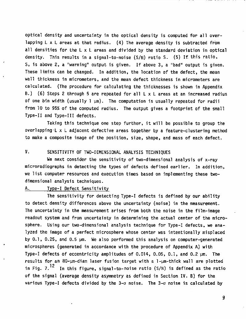
in Fig. 7. 12 In this figure, signal-to-noise ratio (S/N) is defined as the ratio

of the signal (average density asynmetry as defined in Section IV. B) for the

various Type-I defects divided by the 3-u noise. The 3-0 noise is calculated by

9

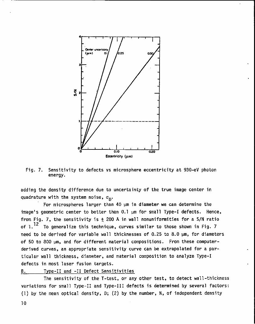
Fig. 7.

adding the

quadrature

4 I I t I

-tintwuncwtointy(pm) 0.1

3 -

z-2 —U1

I —

o0 0.10 azo

Sensitivityenergy.

Eccentricity (/Lm)

to defects vs microsphere eccentricity at 930-eV photon

density difference due to uncertainty of the true image center in

with the system noise, CD.

For microsphere larger than 40 pm in diameter we can determine the

image’s geometric center to better than 0.1 pm for small Type-I defects. Hence,

from Fig. 7, the sensitivity is t 2001k in wall nonuniformities for a S/N ratio

of 1:2 To generalize this technique, curves similar to those shown in Fig. 7

need to be derived for variable wall thicknesses of 0.25 to 8.0 pm, for diameters

of 50 to 800 pm, and for different material compositions. From these computer-

derived curves, an appropriate sensitivity curve can be extrapolated for a par-

ticular wall thickness, diameter, and material composition to analyze Type-I

defects in most laser fusion targets.

B. Type-II and -II Defect Sensitivities

The sensitivity of the T-test, or any other test, to detect wall-thickness

variations for small Type-II and Type-III defects is determined by several factors:

(1) by the mean optical density, D; (2) by the number, N, of independent density

10

.

.

.

.

measurements; (3) by the readout system noise, CD, derived from Fig. 3 and Eq. (l);

(4) by the mean energy of the incident x rays; (5) by the radial location of the

defect from the center of the microsphere image, and (6) by the change in optical

density per unit change in wall thickness, dD/d!L. We have plotted dD/dkversus

photon energy in Fig. 8 for 1.5-~m-thick glass at various exposure levels on HRP

emulsion. These factors result in an uncertainty in the wall thickness, 3og,

which limits the precision of the measurements of average glass thickness. The -

calculation of 30. is defined below:5,13L

For example, a 100-pm-diam

3aR = 3(dD/d!@aDN-1/2um

. (2)

microsphere with a material thickness of 1.5 pm (0.75-

pm-thick wall) exposed to 3300 photons of

results in D = 0.55, OD= 0.043 (Fig. 3);

fore, in 3UR = 0.43/fipm. For our case,

is related to the area scanned.

CuLa radiation per square micrometer

dD/dL = 0.3 ~m-l (Fig. 8), and, there-

in which we step in l-pm increments, N

1.4 I I I I I I I I

I

I I I I I I I

Glass thickness,1.2- 1.5~m

1.0–

z<~ 0.8-.

~ 0.6–

nu

0.4-

0.2-

04 I

102

Exposure(photon@m2)

,n,

~ .“

I..”

) I I 1 I I

103 104

Energy (eV)

Fig. 8, Contrast as a function of energy.

Eleven microsphere were analyzed by using the calculation defined in

Section IV. B for detecting defects with ratios of S above 2. We chose glass

microsphere for this analysis to compare the sensitivities of the radiographic

and optical interference techniques. The calculation was performed for7-by 7-pm

areas (Fig. 6) from 10 to 95% of the microsphere’s radius. The annulus over

which each calculation was performed was stepped radially outward in l-~ steps.

Note that the sampling aperture and the step size should be of the same size as

the defect for which greatest sensitivity is required. These criteria will gen-

erate the greatest efficiency in total sampling time. Our calculation detected

Type-III defects violating the S ratio of 3, defined in

fects ranged from +300Aat 18% of the radius to -1000

These results allow a coarse comparison of the

sphere LB1l (one of the defects for S > 3, Table I), at

Section IV. B. These de-

Rat 85% of the radius.

+300-11 defect in micro-

18% of the radius, with

TABLE I

NUMBER OF TYPE 11 ANDIII DEFECTS

Sample and Number of DefectsExposure Date S2=32<S<3. —

LB1-7-15-77 6 1

LB2-7-15-77 4 0

LB3-7-15-77 o 0

LB4-7-15-77 o 0

LB5-7-15-77 4 0

LB6-7-15-77 3 1*

LB7-7-15-77 NIA N/A

LB8-7-15-77 8 1

LB9-7-15-77 1 0

LB1O-7-15-77 1 0

LB11-10-13-77 19 3

* Excluding bad radiographic area.N/A Not available.

the 3ak limit of Eq. (2). Microsphere LB1l was approximately 335 pm in diameter

(Table II) with a wall thickness ranging between O.76andl.24vm (Table III)

depending on the measuring technique used. The microsphere was exposed to

12

/

.

.

TABLE II

COMPARISON OF DIAMETER MEASUREMENTS

Sample Diameter (m)Sample and Two-DimensionalExposure Date Analysis Interferometry

LB1-7-15-77 179 179

LB2-7-15-77 183 184

LB3-7-15-77 153 151

LB4-7-15-77

LB5-7-15-77

LB6-7-15-77

LB7-7-15-77

LB8-7-15-77

LB9-7-15-77

LB1O-7-15-77

LB11-10-13-77

181

179

186

180

180

172

176

339

184

177

185

177

179

171

174

334

TABLE III

COMPARISONOF WALL-THICKNESSMEASUREMENTS

Wall Thickness (Pm)Sample and Two-DimensionalExposure Date Analysis Interferometry Ratio

LB1-7-15-77 1.14

LB2-7-15-77 1.11

LB3-7-15-77 0.72

LB4-7-15-77 0.98

LB5-7-15-77 1.00

LB6-7-15-77 1.00

LB7-7-15-77 N/A

LB8-7-15-77 0.98●

LB9-7-15-77 1.03

LB1O-7-15-77 1.11

LB11-10-13-77 1.24

N/A - Not available.

1.37

1.44

0.84

1.56

1.19

1..23

1.05

1.21

1.28

1.55

0.76

1.20

1.30

1.17

1.59

1.19

1.23

N/A

1.23

1.24

1.40

0.61

13

- 8600 photons/pm2 of CuLa radiation, This resulted in a central-density, D, of

0.81, and therefore in auDof 0.052 (Fig. 3). Ifwe assume that the dD/d!l curves

in Fig. 8 are approximately applicable for microsphere LB1l, then an exposure of

8600 photons/pm2yields a dD/d!Lof 1.0. These parameters substituted into Eq. (2)

result in 3ak = 0.156/fipm (good for the central area only). The area used in,

the defect detection was 49 pm2 and, therefore, 3U2 was about t 225 A. Comparison.

of the + 300-A detected defect with the t 225-A detection limit implies that the

two-dimensional radiographic image analysis technique can detect Type-III defects.

very close to the theoretical limit, 302, in the central area.

The larger Type-II defects can be detected by using Eq. (2) and the tech-

nique of Appendix B, which converts the center optical density to thickness. If

the center 4% of the microsphere, LB1l, in the previous example,was used to cal-

culate a 30R, the value of Eq. (2) would be f 75 A. Therefore, a Type-II defect

is detectable if several views have a cehtral thickness that varies by more than

f 75 ii. An additional method for detecting large Type-II defects is a trend

analysis of the rim radius used in Type-I defect analysis.

We have outlined in preceding sections several techniques that can be

used to determine three classes of defects. Quantitative results at present can

be obtained only for glass microsphere over a limited range of wall thicknesses,

diameters, and compositions. To increase the robustness of these techniques re-

quires: (1) A complete set of dD/d!L-vs-energy curves (Fig. 8) for various mater-

ials and thicknesses (e.g., 0.25 to 8.0 pm); (2) a recalibration of the root-

mean-square (rms) film noise, CJD,versus film density (Fig. 3; this should be

done periodically); (3) a set of sensitivity curves (Fig. 7) for targets of vari-

ous diameters; and (4) a step tablet calibration for HRP emulsion over an optical

density range of 0.0 to 3.0 on the PDS microdensitometer.

To analyze all three classes of defects, we have implemented algorithms

on our CDC 7600. For an original 128-by-128, 8-bit gray-level laser fusion tar-

get image, the processing time is about 8 to 10s. For 256-by-256 and 512-by-512

images, the processing time is 40 and 160 s, respectively.

VI. COMPARISON OF EXPERIMENTAL RESULTS

We will now describe the quantitative results of the techniques we have,

described and will compare the results of some of these techniques with those of

other image-analysis systems. These systems are: (1) two-dimensional computer

analysis using digitized radiographic data from a PDS microdensitometer, (2) an

14

analog video system from Interpretation Systems, Inc. with a large-magnification

microscope for input of the radiographic data, and (3) a Jamin-Lebedev optical

interferometric measuring system, also using a large-magnification microscope for

input. Our data base is a set of eleven microsphere that were radiographed with

CuLa radiation.AWe will describe: (1) the size of Type-I defects that can be detected

with the three systems, (2) the results of identifying Type-II and Type-III de-.fects using the statistical outlier techniques, and (3) the optical interfero-

metric measurements of diameter and central thickness of the radiographed micro-

sphere made with the two-dimensional computer analysis technique.

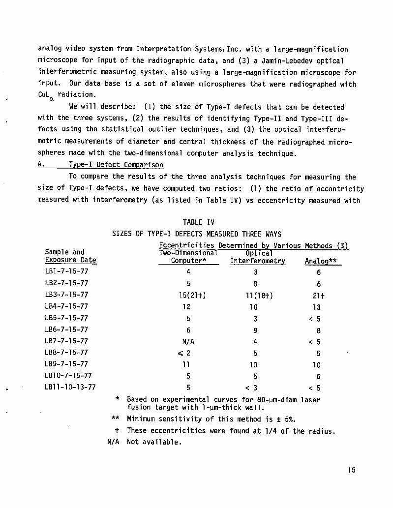
A. Type-I Defect Comparison

To compare the results of the three analysis techniques for measuring the

size of Type-I defects, we have computed two ratios: (1) the ratio of eccentricity

measured with interferometry (as listed in Table IV) vs eccentricity measured with

TABLE IV

SIZES OF TYPE-I DEFECTSMEASUREDTHREEWAYS

Sample andExposure Date

LB1-7-15-77

LB2-7-15-77

LB3-7-15-77

LB4-7-15-77

LB5-7-15-77

LB6-7-15-77

LB7-7-15-77

LB8-7-15-77

LB9-7-15-77

LB1O-7-15-77

.’ LB11-10-13-77

Eccentricities Determined by Various Methods (%)Two-Dimensional Optical

Computer* Interferometry Analog**

4 3 6

5 8 6

15(21t) ll(18t) 21*

12 10 13

5 3 <5

6 9 8

N/A 4 <5

<2 5 5-

11 10 10

5 5 6

5 <3 <5

* Based on experimental curves for 80-pm-diam laserfusion target with l-pm-thick wall.

** Minimum sensitivity of this method is * 5%.

t These eccentricities were found at 1/4 of the radius.

N/A Not available.

15

the two-dimensional computer technique, and (2) the ratio of eccentricity measured

with optical interferometry vs eccentricity measured with the analog-image ana-

lyzer. These results are plotted in Fig. 9. Only Type-I defects in excess of

t 500 Jlwere considered because this size is approximately the limit of sensi-

tivity of both the analog-image analyzer and the optical interferometric measure-

ments. However, there are phase-sensitive interferometry techniques that have

been shown to be sensitive to t 100 A.14’15

For the two-dimensional computer analysis technique the average ratio is

0.99 A 0.37, whereas for the analog-image analyzer the ratio is 1.02 + 0.30.

Thus, the two-dimensional computer analysis technique detects eccentricities as

small as those detected by the best limit sensitivity of the interferometric and

analog-image-analyzer techniques.

While optical interferometry provides a means of quick inspection of op-

tically transparent targets, the two-dimensional analysis of radiographic images

is a sensitive means of measuring defect sizes even in optically opaque materials.

B. Type-II and -III Defect Results

As discussed in Section Y.B, smaller Type-II and Type-III defects were

detected with an outlier technique using the statistical T-test. The total num-

ber of defects with S-ratios between 2 and 3, and above 3, are listed in Table I

for each of the 11 microsphere. Figure 10 indicates by square boxes the positions

2.0 1 I 1 I 1 I

1.5 -

00

.g ,0 0-------------- 4--- AWOIJ4=0.99

@o 0

0.5 -

0 . I I ! I I I

LB2 LB3 Ld4 L% L29 LBIO

Microsphere No.

Fig. 9a. Type-I defect ratios for two-dimensional analysis.

I .5

10

0

~ ,.0 -------- o-+-----l,ozl,oz

o0

0.5

o~U2L84L26L28L29LBt0

Micmphora Na

Fig. 9b. Type-I defect ratios foranalog-image analyzer.

.

.

.

16

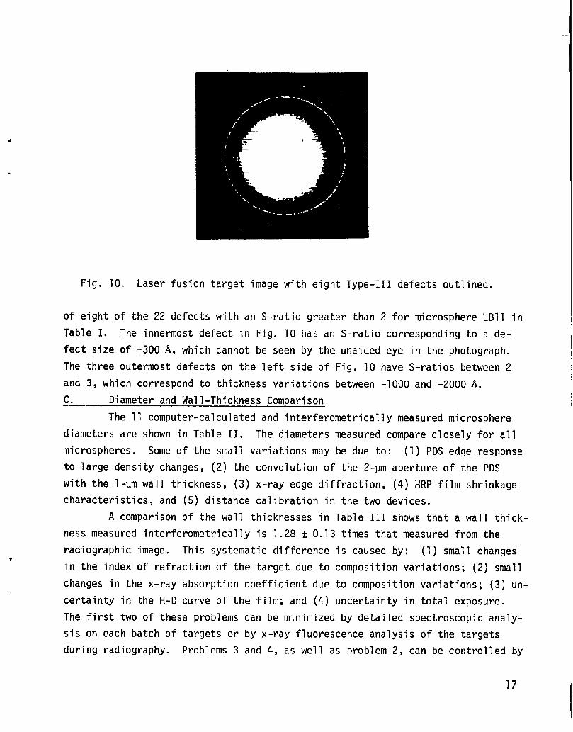
Fig. 10. Laser fusion target image with eight Type-III defects outlined.

of eight of the 22 defects with an S-ratio greater than 2 for microsphere LB1l in

●

Table I. The innermost defect in Fig. 10 has an S-ratio corresponding to a de-

fect size of +300A, which cannot be seen by the unaided eye in the photograph.

The three outermost defects on the left side of Fig. 10 have S-ratios between 2

and 3, which correspond to thickness variations between -1000 and -2000 A.

c. Diameter and Wall-Thickness Comparison

The 11 computer-calculated and interferometrically measured microsphere

diameters are shown in Table II. The diameters measured compare closely for all

microsphere. Some of the small variations may be due to: (1) PDS edge response

to large density changes, (2) the convolution of the 2-urnaperture of the PDS

with the l-~m wall thickness, (3) x-ray edge diffraction, (4) HRP film shrinkage

characteristics, and (5) distance calibration in the two devices.

A comparison of the wall thicknesses in Table III shows that a wall thick-

ness measured interferometrically is 1.28 t 0.13 times that measured from the

radiographic image. This systematic difference is caused by: (1) small changes

in the index of refraction of the target due to composition variations; (2) small

changes in the x-ray absorption coefficient due to composition variations; (3) un-

certainty in the H-D curve of the film; and (4) uncertainty in total exposure.

The first two of these problems can be minimized by detailed spectroscopic analy-

sis on each batch of targets or by x-ray fluorescence analysis of the targets

during radiography. Problems 3 and 4, as well as problem 2, can be controlled by

carefully calibrating each exposure with a step tablet of known step size made of

the same material as the shells.

Careful measurement of the total wall thickness and target diameter is

required to quantify the size of various defects. For Type-I defects it is neces-

sary to know the total wall thickness and target diameter before one can construct

curves as those shown in Fig. 7 to determine the defect size. Similarly, Type-II

and -III defects are dependent on the precision of Fig. 2 and the x-ray absorption

coefficient. When optically opaque laser fusion targets or opaque material layers

are used, we will have to rely totally on these analytical procedures.

VII. IMPROVED IMAGE READOUT SYSTEMS

The sensitivity limit of x-ray microradiography to different types of

defects is more than adequate for present needs and should be acceptable for

future applications. However, to improve the time efficiency of the system, we

foresee the characterization of future laser targets as comprising a multistep

process with each step representing a refinement in the sensitivity to defects.

A trade-off can then be made between the level of acceptable nonuniformity and

the manpower and computational effort expended to characterize the microsphere.

The first step would be visual inspection of the radiographic images for symmetry,

gross wall-thickness nonuniformities, and surface defects. Acceptable targets

would then be radiographed again in three orientations and the images scanned

with an analog-image analyzer to eliminate targets with nonuniformities greater

than 10%. The images of the remaining targets would then be analyzed by computer.

Since many microspheres can be radiographed simultaneously, the initial steps

should represent only a small fraction of the total time needed to characterize

a microsphere.

Three methods of scanning densitometry for the computer analysis were ini-

tially investigated to minimize the total analysis time; they were: 1) flying spot

scanner, 2) camera scanner, and 3) densitometer scanner with an x- and y-stage.

Based on parameters outlined in Appendix C for each scanning system, the flying

spot scanner has the best performance. This is a result of: 1) minimal z-axis

shading correction and x- and y-geometric distortion correction unlike the vidicon

camera system, and 2) not having to mechanically step an x- and y-stage as in the

densitometer system. As a result a careful look at the CYDACflying spot scanning

system at LLL was made. Its main drawback was that it was expensive to build. A

state-of-the-art CCD camera system looks like the best compromise at this time.

18

.

.

It achieves high data rate at relatively low cost while sacrificing analysis

time to make the necessary corrections to the data. However, whichever scanning

system is chosen, maximum utility will be achieved by digitizing the data and

interfacing this readout system directly to a dedicated computer to maximize

throughput.

VIII. CONCLUSIONS

The most important feature of x-ray microradiography combined with two-

dimensional computer analysis is the high level of sensitivity to spherical and

local wall-thickness variations in opaque laser fusion targets. In addition, the

sensitivity of microradiography for optically transparent laser fusion targets is

slightly better than that of most optical interferometric techniques; however,

recently developed phase-sensitive interferometers are more sensitive to wall-

thickness variations.

The sensitivity of x-ray microradiography can be improved by more detailed

scans of the image, by projection radiography, or by averaging the results of many

successive scans to reduce noise. A more complete result for Type-III defects

would include a determination of the defect mass by first determining the area of

the defect using feature-clustering methods. For more robust Type-I defect analy-

sis, the wall-thickness and diameter dependencies of curves similar to those of

Fig. 7 need to be derived. In addition, Moird pattern analysis, two-dimensional

Fourier analysis, and p-0 transformations may provide a higher sensitivity in

some or all classes of defects.

ACKNOWLEDGMENTS

We gratefully acknowledge the aid of the following LASL colleagues:

R. Bagley for performing the scanning densitometry, B. Carpenter for film pro-

cessing, and M. Campbell for devising and implementing numerous clever ways to

mount laser fusion targets. We thank P. Lyons of LASL, P. Bartels of the Univer-

sity of Arizona, and H. C. Andrews of the University of Southern California, for

many useful discussions concerning all aspects of the work reported here.

19

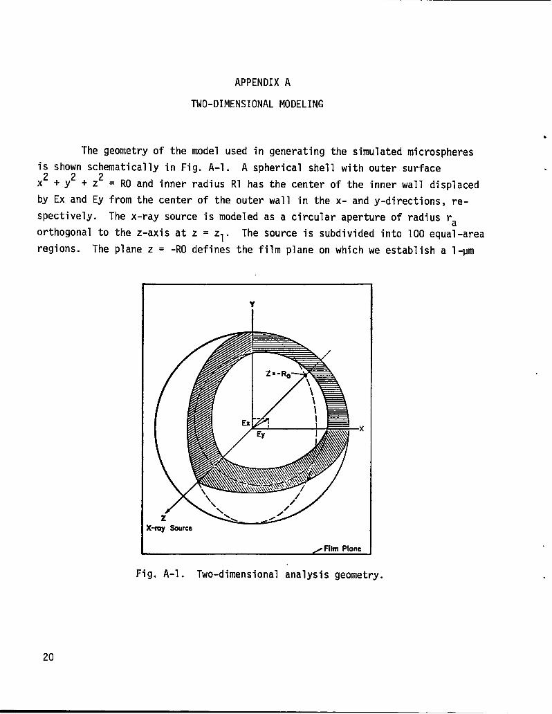
APPENDIX A

TWO-DIMENSIONAL MODELING

The geometry of the model used in generating the simulated microsphere

is shown schematically in Fig. A-1. A spherical shell with outer surface

x2+y2+zL RO and inner radius R1 has the center of the inner wall displaced

by Ex and Ey from the center of the outer wall in the x- and y-directions, re-

spectively. The x-ray source is modeled as a circular aperture of radius ra

orthogonal to the z-axis at z = Z1. The source is subdivided into 100 equal-area

regions. The plane z = -RO defines the film plane on which we establish a l-~m

Y

C-my Source

/Fihn Plane

●

✎

Fig. A-1. Two-dimensional analysis geometry.

20

● ✌

square grid of pixels (image or picture elements) sufficient to cover the image.

Each grid point is subdivided into a 0.1- by O.1-pjnsubgrid, and the transmission

through the target t(k,E) is computed at each point on the subgrid as the average

transmission for each of the 100 source points.

The transmission is derived by calculating the length of target material

between each subgrid point and each source point and then multiplying this thick-

ness, d(k,k,m,n,), by the known x-ray absorption coefficient, u, for the target

material:

10

t(k,i) = ~e-uxd(k’k’m’n) . (A-1)m,n=l

The transmissions at each subgrid point are then averaged to generate the average

transmission T(i,j) for each pixel.

For an initial photon flux, Ho, the mean optical density in each pixel

can be determined by calculating the flux in each pixel (H(i,j) = HO “ T(i,j)),

and referring to Fig. 2 of the body of the report, converting photon flux

to optical density. This procedure creates the simulated radiographic target

images upon which the sensitivity analysis is performed.

The

micrometers

(1)

(2)

(3)

(4)

APPENDIX B

RELATION OF MEAN OPTICAL DENSITY TO MATERIAL THICKNESS

procedure for converting the mean optical density to thickness in

for a specific material involves the following steps.

Determine the x-ray exposure H for a given optical density, D,

from the H-D curve (Fig. 2).

Determine the x-ray exposure Ho that corresponds to the background

density Do.

Calculate the x-ray absorption coefficient, u(E), of the material

used from the absorption coefficients of Henke16 (Fig. B-l).

The thickness, T, of the material is given by

‘=+ ’n(H’Ho)“(B-1)

27

“’E—————7

‘dCa L3 Edge

/

0.346keV

O K Edge0.532 keV

SiK Edge

Co K Edge4.037 keV

# - 1 1 t I 1111 ! 1 1 ! I !

*2 ~3 10’

Energy(eV)

Fig. B-1. X-ray absorption coefficient vs energy for a typical batch ofmicrosphere.

This procedure can be reversed to obtain optical density, as was

III and IV in which computer-simulated laser fusion targets were

analyzed.

done in Sections

computed and

APPENDIX C

THREE SCANNING SYSTEM PARAMETERS

A list of the important parameters about each scanning system follows.

1. Flying spot scanner

a) spatial resolution -0.3 pm

b) z-axis shading - 0.1%

c) x- and y-geometric distortion - 0.1%

d) scanning speed> 10 Mhz

e) field of view - 700 micrometers

f) adjacency effects - small

22

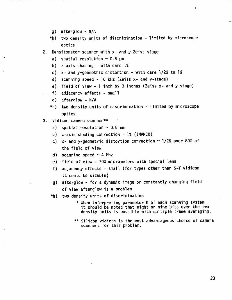
I

●

g) afterglow - N/A

*h) two density units of discrimination - limited by microscope

optics

2. Densitometer scanner with x- and y-Zeiss stage.

a) spatial resolution - 0.5 ~

b) z-axis shading - with care 1%

c) x- and y-geometric distortion - with care 1/2% to 1%

d) scanning speed - 10 kHz (Zeiss x- and y-stage)

e) field of view - 1 inch by 3 inches (Zeiss x- and y-stage)

f) adjacency effects - small

g) afterglow - N/A

*h) two density units of discrimination - limited by microscope

optics

3. Vidicon camera scanner**

a) spatial resolution - 0.5 Mm

b) z-axis shading correction- 1% (IMANCO)

c) x- and y-geometric distortion correction - 1/2% over 80% of

the field of view

d) scanning speed ‘4 Mhz

e) field of view - 700 micrometers with special lens

f) adjacency effects - small (for types other than S-T vidicon

it could be sizable)

g) afterglow - for a dynamic image or constantly changing field

of view afterglow is a problem

*h) two density units of discrimination

* When interpreting parameter h of each scanning systemit should be noted that eight or nine bits over the twodensity units is possible with multiple frame averaging.

** Silicon vidicon is the most advantageous choice of camerascanners for this problem.

-.

23

REFERENCES

1.

2.

3.

4.

5.

6.

7.

8.

9.

10.

11.

12.

13.

14.

B. W. Weinstein, J. App. Phys. 4&, 5305 (1975).

B. W. Weinstein, C. D. Hendricks, “Interferometric Measurement of LaserFusion Targets,” Lawrence Livermore Laboratory Report UCRL-78477 Rev. 1.

T. M. Henderson, D. E. Cielaszyk, and R. J. Sims, Rev. Sci. Instrum. 48_,835 (1977).

R. H. Day and E.J.T. Burns, Adv. X-ray Anal. ~, 597 (1976).

R. H. Day, T. L. Elsberry, R. P. Kruger, D. M. Stupin, and R. L. Whitman,“X-ray Microradiography of Laser Fusion Targets,N Proc. of the Eighth Int.Conf. on X-ray Optics and Microanalysis, Boston, Massachusetts, August 1977.

B. L. Henke, Tech. Rep. No. 4, AFOSR Contract No. AF 49(638)-394,unpublished (1961).

B. W. Weinstein, D. L. Willenborg, J: T. Weir, and C. D. Hendricks, “4TInterferometric Measurements of Laser Fusion Targets,” Proc. of TopicalMeeting on Inertial Confinement Fusion, San Diego, California, February 7-9,1978, Opt. Sot. of Amer., 78CH131O-ZQEA, p. TuE9-1.

H. C. Andrews and B. R. Hunt, Digital Image Restoration (Prentice-Hall,New York, 1977), pp 20-23.

R. E. Moore, Mathematical Elements of Scientific Computin~(Holt, Reinhartand Winston, New York, 1975).

D. M. Hirmnelblau, Applied Nonlinear Programing (McGraw-Hill, New York, 1972).

Frank E. Grubbs, “Procedures for Detecting Outlying Observations in Samples,”Technometrics ~, No. 1, pp 1-2, February 1969.

R. L. Whitman, R. P. Kruger, R. H. Day, and D. M. Stupin, “Two-DimensionalComputer Modeling and Analysis of Thin-Wall Microsphere,” Proc. of theTopical Meeting on Inertial Confinement Fusion, San Diego, California,February 7-9, 1978, Opt. Sot. of Amer., 78CH131O-ZQEA,p. TuE13-1.

D. M. Stupin, R. H. Day, R. L. Whitman, and R. P. Kruger, “Microradiographyof Laser Fusion Targets with Monochromatic X-rays,” ibid, p. TuE12-3.

P. O. McLaughlin and D. T. Moore, “Laser Fusion Microballoon CharacterizationUsing a Single-Pass AC Interference Microscope,” Abstract No. TUQ16, Meetingof the Opt. Sot. of Amer., Toronto, Canada, October 1977. (Gradient IndexLab. Report. No. GIO-10, The Institute of Optics, University of Rochester,Rochester, New York).

24

15. G. W. Johnson and D. T. Moore, “Design and Construction of a Phase-LockedInterference Microscope,” The Sot. of Photo-Optical Instrumentation Engineers,10&, Systems Integration and Optical Design II, 76 (1977).

16. B. L. Henke and E. S. Ebisu, Adv. X-ray Anal. ~, 150 (1973).

25

.

Rinl.xl inthc UnitMiSlmsof Amcriu. Avsibhh. komt&tbml Tcchniul Information .%+.x.

us t3qrarrnwm OrcOmmmLT

528S Purl R0y4! Road

sWi@W~. VA 22161

Miwol%hc s3.00

IX31432S 4.00 , ~~, -$0 7.15 231-27s I 0.75 37640 I 3.00 sol .s2s 1S.2So~~~ ,.~ 1s1-17s H.oll 276-300 11.00 40142s 13.2s 5~6.550 1S.so0s1’07s S.M I 76-XE3 9.no 201-32s I 1.7s 4264S0 14.00 SsI -s7s 16.2S076-[ 00 6.00 ?01-225 9.25 3~6.3so I 2.on 4s147s 14s0101-12s

S76-6006.S0

16.S0226-250 9.s42 151-375 I 2.s0 476.S00 15.00 M71.up

Mu: Add S?.50 (or UCII xldtlional IIWW mc?mcnt [mm 601 pgc. up.