LA-6824LGi?OanduC-32

Issued:FebruatY1978

CIC-14 REPORT CCXLECTiONREPRODUCTION

COPY

System of Nonlinear Partial Differential Equations

I Describing Cylindrical Plasma Collapse

I

}

Iamo

AlfredCarasso*B.R.Suydam

*Visiting Staff Member.

Department of Mathematics and StatisticsUniversity of New MexicoAlbuquerque, NM 87131

sscientific laboratory

of the University of CaliforniaLOS ALAMOS, NEW MEXICO 87545

Ii

An Affirmative Action/Equal Opportunity Employer

uNITED STAT?=

DEPARTMENT OF ENERGY

cONTRACT W-7498-ENG. 36

A.Carasso’sworkwassponsoredby theArmy ResearchOffice,GrantNo.DAAG29-76-G43153.

Ptmwl m 11,. I!mt.d St.Ie$ of Ameti.., Avil.hlc tntmN.mm.d Tcchnkal lnfmm.tion Scrvi.c

US. 12qmrtmcnt of CummcwcS28S Put! R,,yd RuddSpringlidd. VA 22161

Ml’ Itd-ldlc s J.lm 126.1S11 1.2s001.I12S

251.275 10.7S 316-4004.no 1s1.11s 8.(10 276.300 1! .00 401425

026.050 4.s0 176->0(1 9.00 301.325 11.7s 4264S0051-07s S.25 201-225 9.23 326-3S0 12.lfIl 45147s076.100 6.00 226-2S0 9.s0 351-37s 12s0 476.S011101.125 6.S0

1. Add S2.S0 (or edf additlond Ioo.pqe increment from 601 P%$up.

I 3.c41 SO1.S2S!s.2s13.2S S26-SSO 1s.s014.00 SSI-S75 162514 .W1 576-60u 16.5015.IM1 601 Up --1

a

*

‘3%1sWD..I w.. Pmp.red 8s ●n .cco..t .[ work w..s.xedby Ihv United Sut.s Government. N.tthcr the Umlcd Slmtesnor the Umled Slate. IMmrcmrrnt 0/ Fker:v. nor .IZY “1 thclrc.mplo> ..s, nor .w .1 then .ontr--tms. subcu. tr.. w- Orth.ir employeex m.ke. an. wum”ty. .X P?.S or tmnh.d. O..smmcs urw I.SA h.bthty Ur mmonobd,lY f., Ih. .C.UW’Y.conwlete. c.s. w ..tf.lne*s of ●ny Inlt, rm. twn. apfur.lus.wsducl. 0, PWC.U d!u’1’m’d. or ,, P,, w”l’ ch.t ,fs “s, % ,“,1,1not mfrtnue PrIL’.1e1Yowned nshu.

A SYSTEN OF NONLINEAR PARTIAL

DIFFERENTIAL EQUATIONS DESCRIBING CYLINDRICAL PLASMA COLLAPSE

by

Alfred Carasso and B.

ABSTRACT

R. Suydam

We consider the snow-plough model for describingcylindrical plasma collapse for a specified constantdriving term. This coupled nonlinear system consistsof five partial differential equations in two independ-ent variables, one of which is the time variable.Generally, the initial value problem for similar systemsis improperly posed. However, here we show thatby

— direct construction of the unique solution, explicitly

N ~in terms of the initial data, the solution exists for~~~~all positive times and is generally an infinitely dif-~~:r-ferentiable function of the independent variables.<~o~‘~~E” Nevertheless, the solution always develops a nonphysical;= ;--”singularity after a certain positive time, and there-

~ after ceases todescribe theunderlying physical situa-Our theory leads to an a“priori bound in terms

of the initial data, on the tti-einterval during which~=~~ the snow-plough model is physically realistic. We==m’--r- .- —discuss.several examples which illustrate the pathol-,.

.; ogies exhibited by the solution.

1. INTRODUCTION

The underlying physical problem considered in this report is the com-

pression of a fully ionized plasma by a magnetic piston. Because a fully

ionized plasma is normally a very good conductor, we may set the resistivity

equal to zero. The magnetic field then cannot penetrate into the plasma; it

simply drives the sharp plasma-vacuum interface like a piston. To treat

this problem properly, one should solve the hydromagnetic equations in the

plasma for the magnetically driven shock. This shock ulttiately reaches the

center of the plasma and is reflected back to the piston. In this report we

1

are concerned with the early phase of the compression, that is, before arrival

of the back shock. In this case, the piston motion can be well approximated

by a simplified model, the “snow-plough” equations,1,2

and one can avoid the

more formidable problem posed by the full hydrodynamical equations. Thus ,

instead of following the development of the shock, we assume that each plasma

element remains undisturbed until the piston arrives. When the piston ar-

rives, each plasma element is picked up and sticks to the piston face. We

thus imagine the shock to remain infinitesimally close to the piston in this

approximation and assume the shock compression of the plasma is infinite.

Although these approximations are somewhat crude, the snow-plough model

has proved useful in plasma compression calculations. Recently, Nelson,

Brown, and Hart2 described a code used for numerical computations of such

problems. They reported that the code, based partly on the snow-plough model,

runs well and gives good results.

In Sec. 2, we derive the snow-plough equations directly from the prin-

ciples of mass and momentum conservation for the two-dimensional case of a

cylindrical plasma. These equations form a nonlinear system of five partial

differential equations in two independent variables. This set of equations

can also be obtained from the full hydrodynamical equations as a limiting

case, when the temperature approaches zero and y (the ratio of specific heats)

approaches unity.

This simplified system of snow-plough equations is the basis of our

study . These equations are highly unconventional, and the model raises new

mathematical questions. The initial value problem for similar systems is

generally improperly posed. In fact, a linearized stability analysis of the

snow-plough equations reveals that the growth rate of perturbations becomes

infinite as their wavelength approaches zero. Yet, surprisingly, the algo-

rithm discussed in Ref. 2 encountered no stability difficulties—an apparent

contradiction to a well-known principle in numerical analysis.3

In this

report we take the first step toward answering these questions. We shall

show that for a specified constant driving term, the nonlinear initial value

problem is well-po seal,and we shall construct its unique solution explicitly

in terms of the initial data. The solution will exist for all t > 0. Never-—

theless, as will be shown, the solution always develops a nonphysical singu-

larity after a certain positive time, Tc, and thereafter ceases to describe

the underlying physical situation. This is so despite the fact that the

solution is generally an infinitely differentiable function of the independ-

ent variables. In fact, our construction leads to an upper bound, which

may be calculated explicitly in terms of the initial.data, for the time in-

terval during which the snow-plough model is physically realistic. In Sec. 5,

we discuss examples which illustrate these points~ as well as further compli-

cations not covered by our theorems.

The above problem is a particular instance of the more general problem

of moving a simple? closed plane curve according to some prescription. This

type of problem occurs in various physical situations. For example, optical

problems may be formulated in this fashion, the plane curve (or, more general-

ly, surface) being an isophase front. With proper rules for moving the curve,

diffraction and even nonlinear optical effects can be fully accounted for;

also, such a formulation has attractive computational features. Our ultimate

aims, therefore~ are broader than the snow-plough problem discussed in this

report.

As a simple example of the above general class of problems, consider

the evolution of a curve when each point on the tune is moved toward the

instantaneous inward noxmal, at a uniform velocity, which we may normalize

to unity. Let the curve be given parametrically by

x = X(a,t), y = Y(a,t),

and let the element of arc length, ds, be given by

ds = SdA, S E[t~x)’ + (%y)’]1/2 ,

(1.1)

(1.2)

awhere , ~

A K“

Then, the e“@ations of motion for the curve are

(1.3)

The initial value problem is well-po sad for this nonlinear system. How-

ever, if S were simply a function of (X,Y,A,t), the initial value problem

would probably be ill-posed because these equations constitute a generaliza-

tion of the Cauchy-Riemann equations.

Although we have not found a method of generally classifying such systems,

these problems have the following property in common. In their natural form,

the equations are not quasi-linear. When, by introducing new dependent var-

iables, they are quasi-linearized as

Aathqz=c, (1.4)

the matrices A, B, and C are highly singular.

2. DERIVATION OF THE SN(X+PLOUGH EQUATIONS

Let (X1,X2,X3) denote Cartesian coordinates. We consider a cylindrical

plasma with its axis along the X3 coordinate so that

~ (anything) = O .ax

The plasma-vacuum interface can be described as a simple closed curve,

r = I’(t), in the (X1,X2) plane. This curve is given parametrically by

(2.1)

.

,

X1 = R(x,t)

4

(2.2)

and

x’ = Z(x,t), (2.3)

where t is time and x is a conveniently chosen parameter such that O ~ x < 21T.

Thus, R and Z are 21T-periodic functions of x. We choose x to increase anti-

clockwise

are given

and

around I’. The unit tangent ?(x,t) and the unit normal ~(x,t) to r

by

()= 1/S Rx, T2 =

‘1()

1/s 2X,

‘N - t’s)’”‘= t’s)‘x’where

s=(R:+‘V1’2“

(2.4)

(2.5)

(2.6)

The convention chosen for x makes ~(x,t) point inward into the plasma. Let

us revert momentarily to three dimensions and consider an element 6X of the

interface with velocity ~. Then, in time 6t, 6X sweeps up a volume (to;)6Z.

Let p be the constant plasma volume density and p be the mass per unit area

of the piston, that is, mass of plasma already swept up. Then, because 6X

= S6X36X, mass conservation is given by

Mt

= ps(fi”:), (M= @). (2.7)

Similarly, if II> 0 is the jump in total pressure across the plasma-vacuum

interface, momentum conservation is given by

5

(Ma~ = k.

WithB = (U,V), we also have

Rt=U, Zt=V.

Once 1 is specified, Eqs. (2.7),(2.8),and (2.9)are the equations

motionof the piston,that is, the curve1’. Herewe consideronly

(2.8)

(2.9)

of

the

casewhereIIis a constantspecifieda priori. Generally, the plasma may—

have a “frozen in” magnetic field,BP2, in additionto its pressurep.

Then,IIis givenby

‘=%[k’c)2-8’121-p‘(2.10)

where B~ac must be computedfrom givenexternalcurrentsand boundarycondi-

tionson the movingcurveI’. We hope to considerthis latterproblemin

futurework.

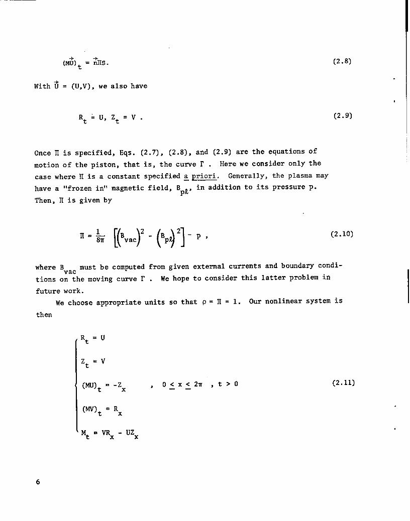
We chooseappropriateunits so that p= II= 1. Our nonlinearsystem

then

is

Rt =U

zt=~

(Mu)t= -Zx , o<x<21r, t>o-—

(MV)t= Rx

Mt = VRx - Uzx

(2.11)

6

whereall fiveunknownsare functionsof x and t, and 27rperiodicin the

spacevariablex.

Here we describethe initialconditionsto be adjoinedto this system.

Let u denotea genericpositiveconstant,not necessarilyhavingthe sameval-

ue at differentoccurrences.We assumethe initialinterfaceto be a smooth,

simpleclosedcurvewith a continuouslyturningtangentso that

(2.12)

0< X<2T. We also assume——of positionalongthis curve

everypoint (Fig.1). Thus,

‘-J- -

the initialvelocityto be a continuousfunction

and to be directedinwardintothe plasmaat

with n, and n. as in (2.5),J. &

nl(x,,)u(x,,)+ n2(x,0V(x,0)~u > OS (2.13)

o~x527r. Finally,becausethe mass sweptup by the pistonis initially

zero,

M(x,O)=O, 0~x<27r. —

)(2 1=

(2.14)

3. THE LINEARIZEDINITIALVALUE

D-77’ 1 PROBLEM

u“ It is instructiveto studythe ev-

olutionarityof a linearizedversion

of (2.11). Considerthe lastthree

ICHI,/

i

)(3

Fig. 1. Initial plasma-vacuum interface.

equationsin (2.11),namely,

{

‘= -($‘c (?‘tVt=(;)Rx-(;)Mt ,3.1,

Mt= VRX - UZX .

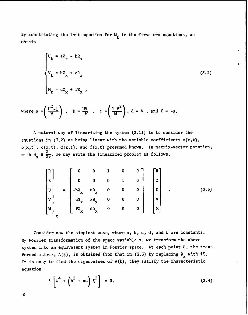
By substituting the last equation”for Mt in the first two equations, we

obtain

1Ut = aZx - bRx

Vt = bzx + cRx

[Mt = dzx + fl?x ,

wherea =

(3.2)

)I-V2 , ~M

=V , and f = -U.

A naturalway of linearizingthe system(2.11)is to considerthe

equationsin (3.2)as being linearwith the variablecoefficientsa(x,t),

b(x,t),c(x,t),d(x,t),and f(x,t)presumedknown. In matrix-vectornotation,

R-

2

u

v

M..

t

tritethe linearizedproblemas follows.

o 0 1

0 0 0

Ca ba ox x

fa dax ox

simplestcase,

0 0-

10

0 0

00

0 0 !R“

z

u

v

M.

. (3.3)

wherea, b, c, d, and f are constants.Considernow the

By Fouriertransformationof the spacevariablex, we transformthe above

systeminto an equivalentsystemin Fourierspace. At eachpoint ~, the trans-

formedmatrix,A(C), is obtainedfrom that in (3.3)by replacingax with i~.

It is easy to find the eigenvaluesof A(E);they satisfythe characteristic

equation

‘F4+(’’2+ac)c21=0” (3.4]

Equation (3.4) shows that2

if, b + ac = O; that is,

. .

the linearizedproblemis well-posedif, and only

if and only if,

Uz(x,t)+ V’(x,t)= 1 . (3.5)

If bz + ac ~ O, A(Q alwayshas one eigenvalueA(E),suchthat

Re A(E) = a~,a>o. (3.6)

In that case,a solutionof (3.3)at t > 0 cannotbe estimatedin termsof-

the initialdata in the L’ norm,nor in most otherusefulmetrics,and the

initialvalueproblemfor (3.3)is improperlyposed,much likethe Cauchy

problemfor the Cauchy-Riemannequations.

In the next sectionwe shallshowthat the nonlinearinitialvalue pro-

blem (2.11)has a uniquesolutionexistingfor all t > 0, and we shallconstruct—this solutionexplicitlyin termsof the initialdata. The explicitform of

the solutionshowsthat the latterdependscontinuouslyon the data in the

Lm norm.

4. THE NONLINEARPROBLEM

For givenS > 0, let JS be the rectangle[(x,t)l O ~x:21T, O < t < S]

in the (x,t)plane. Let a(JS)be the linearspaceof all real valuedfunc-

tions,u(x,t),definedand of classC1 on YS, the closureof JS, and whichare

27rperiodicin the spacevariablex.

The nonlinearproblemmay be formulatedanalyticallyas follows. Given

the initialvaluesU(X,O),V(X,O),R(x,O),Z(X,O),and MIx,O),which satisfy

(2.12),(2.13),and (2.14),find a time intervalO St < T and five functions

U(x,t),V(x,t),R[x,t),Z(x,t),and M(x,t)suchthat

(a) U, V, R, Z, M m(JT)

(b) U, V, R, Z, M satisfy(2.11)onJT.

Lemma 1.

In any solutionto the aboveproblem,we have

(4:1)

Proof.

By assumption,a solutionis a C1 functionon ~T for someT > 0 .

In particular,the system (2.11)mustbe satisfiedas t + O . By (2.12),

the unit tangentto the initialcurve,~(x,O),is well definedat every

point. Also,by (2.13),the initialvelocity,fi(x,O),is never zero and is

alwaysto the left of ~ . Hence,on O < x < 2m ,—.

VRX - UZX

()

lf2R: + Z: I ●jbh)>o,.(;xfi) _

t=o

(4.2)

3where~ is a unit vectorin the x direction. Usingthe last equationin

(2.11),we obtain (4.1)from (4.2).

Lemma2.

Let thereexista solutionto the nonlinearproblem. Then,there

existsT* > 0 , suchthat

M(x,t)> 0 on JT* . (4.3)

Proof.

This followsfrom (2.14)and Lemma1.

Lemma3.

Let thereexista solutionto the nonlinearproblemand let T* be

as in Lemma2. Then,

U2 + V2 = 1 , (x,t)GJT*. [(4.4]

.

10

Proof.

From the lastthreeequationsin (2.11),we have

I(Mu) (Mu)t = -Muzx

(MV)(MV)t = MVRX

MMt =MVRX-MUZX .

Hence,

() (M2t= )M2V2 + M*U2 ~ .

Using (2.14)we integrate(4.6)with respectto t to get

[ 1M2(x,t)= M2(x,t) U2(x,t)+ V2(x,t) .

The resultfollowsfrom Lemma2.

Lemma4.

The followingtwo conditionson the initialdata are necessaryfor

existenceof solutions,

and

Proof.

(4.5)

(4.6]

(4.7)

(4.8)U2(X,0)+ V2(X,0)= 1

U(X,O)RX(X,O)+V(X,O)ZX(X,())= O. (4.9)

Equation(4.8)followsfrom (4.4)and continuityat t = O . Equation

(4.9)is a strongerrequirementthan (2.13)becauseit impliesthat the

velocitymust lie along the inwardnormalto the initialcurve; (4.9)

followseasilyfrom the momentumequationsat t = O .

11

Lemma 5.

Knowledgeof U(x,t) and V(x,t) in any rectangle,JT, uniquelydetermines

the otherthreedependentvariablesin JT . We have .

tR(x,t)= R(x,O) +

JU(x,s)ds,

0

t

Z(x,t)= Z(x,o)+I

V(x,s)ds,

0

and

M(x,t)= g(x)II 1

U(x,s)u(x,o) + V(x,s)v(x,()) ds ,

0

[[[

s+ ds

1V(X,S)UX(X,U) - U(X,S)VX(X,U) du ,

where

g (x) = Mt(x,O) =

Proof.

We need only establish

mass equationin (2.11),we

4.

RX(X,O)

w~u>o’

the representation(4.12). Integratingthe

get

1.

M(x,t)=-II

V(X,S)RX(X,S)1

- U(X,S)ZX(X,S) ds .

0

(4.10)

(4.11)

(4.12)

(4.13)

(4.14) .

●

12

From (4.10)and (4.11),we have

.

Rx(x,s) = RX(X,O)+

fUX(X,u)du

and

Js

Zx(x, s) = ZX(x, o) +’ Vx(x,u)du.

0

Next, from the momentumequationsin

Mt(x,O)U(x,O)= -ZX(X,O)

and

Mt(x,O)V(x,O)= Rx(x,()).

(4.15)

(4.16)

(2.11),evaluatedat t = O,

[4.17)

R (xjO)Defineg(x) = ~ . Then, from (4.18)and (4.1),g(x)~0 > 0 ,

and from (4.17),ZX(X,O)= -g(x)U(x,O).By substituting(4.15)and (4.16)

in (4.14),we obtain (4.12).

Lemma6.

Let thereexista solutionto the nonlinearproblemand let T* be as

in Lemma2. Then U(x,t)and V(x,t)are independentof t on JT* .

Proof.

From Lemma3, we have.

[4.18)

. U(x,t)= -Cos e(x,t) (4.19)

13

and

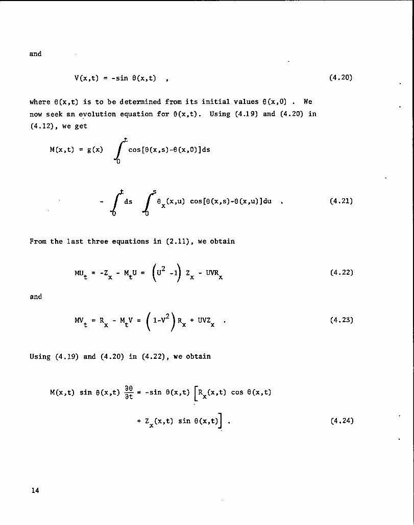
V(x,t)= -sin O(x, t) , (4.20).

wheref3(x,t) is to be determinedfromits initialvalues(3(x,0). We .now seek an evolutionequationfor 9(x,t). Using (4.19)and (4.20)in

(4.12),we get

t

M(x,t)= g(x)1

cos[9(x,s)-(3(x,0)]ds

o

-[ [

ds ex(x,u)cOs[e(x,s)-e[x,u)]du.

From the lastthreeequationsin (2.11),we obtain

~t . -Zx - Mt(J . ()U2 -1 Zx - UvRx

and

()Mvt . Rx - Mtv . 1-V2 Rx + Uvzx .

Using (4.19)and (4.20)in (4.22),we obtain

hf(x,t) sin e(x,t)~ = -sin e(x,t)[Rx(X,t)COS f)(X,t)

1+Zx(x,t)sin e(x,t) .

(4.21)

(4. 22)

(4.23)

(4.24)

.

.

14

Next,we substitutefor Rx and Zx, from (4.15)through(4.18)in (4.24),

to obtain

ao

{M(x,t)sin e(x,t)~= sin e(x,t) -g(x)sin[e(x,t)- e(x,())]

t

+ J }sin[6(x,t)-9(x,s)]ex(x,s)ds .

0

Similarly,startingfrom (4.23),we obtain

ae{

M(x,t)cos e(x,t) ~= cos tl(x,t) -g(x) sin[O[x,t] . e[x,O)]

t

+ I }sin[e(x,t)-e(x,s)]ex(x,s)cls .

0

DefineN(x,t)by

(4.25)

(4.26)

tN(x,t) = -g(x) sin[(3(x,t)-e(x,o)]+

Jsin[f3(x,t)-e(x,s)]ex(x,s)ds. (4.27)

o

Then, (4.25),(4.26)togetheryieldthe followingevolutionequationfor

e(x,t).

aeM(x,t)~= N(x,t) , (x,t) ~ JT* . (4.28)

This nonlinearequationhas a uniquesolutionin JT* , namely,e(x,t)= (3(x,0).

Using (4.21)and (4.27),we observethat

ill= 80 aM(4.29)

at -=% “

15

Hence,from (4.28)and (4.29),

~aN+NaMat z

=0 onJT* . (4.30).

Consequently,from (4.30]and (2.14), .

N(x,t)M(x,t)= N(x,O)M(X,O)= O on JT* . (4.31)

SinceM(x,t)> 0 on JT* , we concludethat N(x,t)❑ O on JT*, and from

(4.28),(3t(x,t)❑ O onJT*. Hence,

U(x,t)= -Cos e(x)

and

V(x,t)= -sin e(x)

as required.

Lemma 7.

Let thereexista solutionto the nonlinearproblemand let T* be as

in Lemma2. Then,on JT* , this solutionis givenby

[

U(x,t)= -COS e(x)

V(x,t)= -sin e(x)

R(X,t)= R(x,O) - t COS 61(X)

Z(x,t)= ZIX,O)- t sin e(x)2

M(x,t)= t g(x) - ~ ex(x) ,

Rx(X,O)whereg(x) =

-V(x,o) –> m > 0 , and e(x) = arc COS[-U(X,O]].

(4.32)

(4. 33)

(4.34)

.

16

Proof.

This followsimmediatelyfrom (4.32),(4.33),and LemmaS.

Lemma8.

Let f)(x)be as in Lemma7. Then,thereexistsan open interval

1 C [0,2m],suchthat

ex(x)>o, xcIo (4.35)

Proof.2

Let ~ and ~be the unit vectorsin the X1 and x directions,respec-

tively,and~(x) be the unit tangentvectorto the initialplasma-vacuumin-

terface. Then,using (4.17),(4.18),(4.32),and (4.33),

?(x) =

=

~ RX(X,O)+ ~ ZX(X,O)

[ 11/2

R~(x,O]+ Z~[x,O)

- T sin e(x)+ J cos e(x) .

Let Y(x) be the anglewhich~(x) makeswith the xl-axis. Then,

+T(X) ● I = cos Y(x) = -sin e(x) .

(4.36)

(4. 37)

Thus ,

Y(x) = e(x) + $ . (4.38)

By hypothesis, the initial interface is a simple closed curve. Hence, the

net increase in Y(x) as x ranges from x = O to x = 2m is exactly2wo

Therefore,

17

21T

1ex(x)dx= e(2T)- e(o)= 2n ,

0

Sinceex(x) is continuouson [0,2T],the resultfollows.

Lemma9.

DefineM(x,t)by

2M(x,t)= tg(x)- ~ex(x) [4.40]

forallO~x ~2mandallt >0. Then,on any rectangleJT , the set of

pointswhereM(x,t)# O is dense.

Proof.

For t > 0 , M(x,t)= O if, and only if,

2g(x)s tex(x) . (4.41)

Sinceg(x)~u > 0, we see from (4.41)thatgivenanyx ~ [0,2m],there is “

at most one positivevalueof t suchthat (4.41)is satisfied. Hence,in

any rectangleJT , the set of pointswhereM(x,t)= O is eitheremptyor

lieson a curve. This provesthe Lemma.

Theorem1.

Let the initialdata satisfythe necessaryconditions,(4.8)and (4.9),

in additionto (2.12),(2.13),and (2.14). Then,thereexistsa unique

solutionto the nonlinearinitialvalueproblem,(2.11). The solution

existsfor all t > 0 and is

Proof.

It is readilyverifi.ed

0<x<2mandallt>0.——

18

givenby (4.34).

that [4.34) is a solutionof (2.11)for all

Accordingto Lemma7, (4.34)is the only

(4.39).

.

.

.

solutionin any rectangle JT* whereinM(x,t)> 0 . An inspectionof the

proofsof Lemmas3, 6, and 7 shows,however,that (4.34)is the only solution

in any rectangleJT in whichM2(x,t)> 0 on a densesubset. By Lemma9,

we concludethat (4.34)is the only solutionto the problemon t > 0 .—

Theorem2.

Let R(x,t)and Z(x,t)be as in (4.34)and let I’(t)be the curvein the

(X1,X2)plane,definedparametricallyby

1x = R(x,t) (4.42)

and

X2 = Z(x,t) , (4.43)

where t is fixedand O < x < 2n .——

DefineTc by

Tc = Inf {1g(x)

}t(x) t(x)~o, t(x) == ,

x =[0,2T] x(4.44)

with g(x) and O(x) as in (4.34). Then Tc > 0 , I’(t)develops a singularity

as t + Tc , and M(x,t)CO for some x c[0,2T] if, and only if) t ~ 2TC .—

Proof.

By Lemma8 and the fact that g(x) > w > 0, the set of pointst(x) suchg(x)

‘hat t‘x)= p and t‘x)~ 0 ‘s ‘ot ‘mpty” ‘ince‘x(x]‘s bounded‘n

[0,21T]and g(x) is boundedaway from zero,the aboveset of points~t(x)}

is alsoboundedaway from zero. HenceTc > 0 . We now show that the trace

of T(t) developsa singularpoint as t + Tc . First,observefrom (4.9)

and (4.34)that for all t > 0,—

19

U(x,t)Rx(x,t)+V(x,t)Zx(x,t)= O .

From the mass equationin (2.11),

Mt(x,t)= V(x,t]Rx(x,t)- U[x,t)Zx(x,t).

(4.45)

(4.46)

Since U2(x,t) + V2(x,t) = 1 , it followsfrom (4.45)and (4.46)that

Rx(x,t)= Zx(x,t)= o , (4.47)

if, and only if, Mt(x,t)= O . From (4.34),we have Mt = g(x) - tex(x) .

Hence,the earliesttime at whicha singularityappearson the plasma-vacuum

interfaceis givenby Tc . Noticethat from (4.41),the earliesttime at

whichM(x,t)= O for somex=[0,21T] is 2TA .L

Theorem3.

(a)Let g(x) - Tcex(x)❑ O on [0,2T]. Then,

whoseradiusshrinksto zero as t + Tc , and

g(x) - Tcex(x)= O at some isolatedpointX.

the traceof I’(t)is a circle

thereafterexpands. (b)Let

● [0,2T]. Then,the trace

of I’(TC)has a continuouslyturningtangentat everypoint,but the radius

of curvaturetendsto zero as x + xo“For sufficientlysmalls > 0 and

all t, suchthat O < (t-Tc)< c , the traceof l’(t)containstwo cusps

near x .0(c)Let g(x)- Tcex(x)= O on someclosedinterval[a,b]properly

containedin [0,2m]. Then,the arc a < x < b on the traceof I’(t),t < Tc——is an arc of circlewhichshrinksto a singlepoint,y, as t 4 Tc, and I’(t)

developsa cornerat y . For t slightlygreaterthan Tc , I’(t)contains

two cusps,one near x = a and the othernear x = b.

Proofof (a).

From (4.9),(4.13),and (4.34),we have

RX(X,O)= -g(x)sin e(x) = -Tcex(x)sin e(x)

20

(4.48)

and

Zx(x,o) = g(x)Cos e(x)= Tcex(x)COS e(X) .

Hence,

R(x,O) =R(O,O) + T=f

-eu(u) sin (1(u)du

o

= R(O,O) + Tc[cose(x) - Cos e(o)] .

Similarly,

Z(x,o) = Z(O,O) + T=[sinEl(x)- sin Cl(O)].

(4.49)

(4.50)

(4.51)

To completethe proofof (a)we substitutein

R(x,t) - [R(O,O) - Tc cos fl(0)]= (Tc-t)

Z(x,t) - [Z(O,O) - Tc sin (3(0)]= (Tc-t)

Proofof (b).

(4. 34) to obtain

Cos e(x) (4.52)

sin e(x) . (4.53)

Let Y(x,t) be the polarangleon I’(t),that is, the anglethe unit tan-

gent to r(t),~(x,t), makeswith the xl-axis. From

? Rx(x,t)+ ~ Zx(x,t):(x,t)=

[ 11[2 ‘ (4.54)

R~(x,t) + Z~(x,t)

and (4.34),togetherwith

RX(X,O) = -g(x)sin e(x) , ZX(X,O) = g(x) cos e(x),

we find

[-sin e(x) g(x)-tex(x)

Cos Y(x,t) = ;(x,t).1= 1k(x)-tex(x)I

(4.55)

(4.56)

21

Now if t ~ T= we have g(x) - tex(x)~ O on [0,2n], and hencefrom 4.56,

Y(x, t) = e(x) + ; .

Also,the curvatureK is givenby

(4. 57)

ex (XI

K(X, t) =

k(x) -

(4.58)tex(x) I “

From (4.57) and (4.58] we see that if g(x)- TcOx(x)vanishesat some iso-

latedpointX. , the traceof I’(TC)has a continuouslyturningtangentat

Xo, althoughthe curvaturethereis infinite.

Next, let s > 0 be sufficientlysmalland let O < (t-Tc)< c . Then

dxo) - tex(xo)< 0, and thereare two points~ and ~, such that ~ < X. < ~ ,

and g(x) - tex(x)changessign at eachof ~ and q. From (4.56),we see that

thesesign changesleadto a jump of m radiansin the polarangleat ~ and ~.

This is the reasonfor the appearanceof the two cuspsnear X. .

Proofof (c).

ConsiderR(x,t)and Z(x,t)for a < x < b and O < t < Tc. We have,——using (4.55),

R(x,O)= R(O,O)-I

g(x) sin e(x)dx+ Tc[cosf3(x)- cos e(a)],

aZ(x,o)= Z(o,o)+

Jg(x) cos O(x)dx+Tc[sin e(x) - sin e(a)].

o

(4.59)

(4.60)

Hence,using (4.34),we have,

R(x,t)= R(O,O)- Tc cos e(a) -f

g(x) cos EI(x)dx+ (Tc-t)sin e(x), (4.61]o

.

.

.

.

22

aZ(x,t) = Z(o,o) - T= sin e(a) +

Jg(x) cos 13(x)dx+ (Tc-t)sin e(x), (4.62)

o a<x <b.——

Thus,as t 4 Tc, we have R(a,t) + R(b,t) and Z(a,t) + Z(b,t), and the arc

a < x < b on the traceof r(t) is an arc of circlewhich shrinksto a single——point,y , as t + Tc . Moreover,from (4.57),we observethat at t = Tc,

the polar angleat y e~eriences a jump equalto f3(b)- e(a)~O,and hence

r(t) developsa cornerat y as t + T=. Subsequently,this cornerevolves

intoan arc of circlewhosecurvatureis oppositeto that when t < T I-Iow-C“

ever,as in case (b) above,therewill be two sign changesin g(x) - tex(x),

for t slightlygreaterthan T , near x = a andx = b, respectively.Hence,c

therewill againbe cuspsat thesepoints. This completesthe proofof

Theorem3.

Theorem4.

The uniquesolution(4.34)to the nonlinearinitialvalue problem (2.11),

althoughit existsfor all t ~ O, is not relevantto the underlyingphysical

problemfor t ~Tc .

Proof.

Let p(x,t)be the densityof mass sweptup by the pistonas in (2.7),

and let S(x,t)=[R~(x,t) + Z~(x,t)]l/2 as in (2.6). Theorem2 guarantees

the existenceof a pointxc in [0,21T],suchthat S(xc,t)tendsto zero as

t+Tc , whileM(x,tc)~u> O on [0,2’Ir].Hence,since u = h4/S,we have

U(xc,t)~~ as t + Tc, a physicalimpossibility.

Remarks.

The quantityT- is an upperboundon the time intervalduringwhich the

snow-plough

pistonwill

well before

shock-shock

L

model is physicallyrealistic. In a real plasma,a magnetic

drivea shockwhichalwaystravelsfasterthan the piston. Thus,

Tc, the shockfrontwill developsingularitieswhich lead to

interactions.These interactionsgeneratea signalin the shocked

materialwhich travelsback to the piston. The back signalmodifiesthe mag-

neticpistonbehaviorin a mannernot includedin the snow-ploughmodel.

Thus, eventhoughthe solutionis completelyregularup to t = T=, the model

breaksdown somewhatearlier.

23

5. EXAMPLES

The simplestexampleof a solutionto the nonlinearproblemoccurswhen

the initialinterfaceis a circle. Let AO > 0 and let

R(x,O) = A. cos x, Z(X,O)=Ao sinx,

U(x,O)= -cosx, V(x,O)= -sinx,

M(x,O)= O,

whereO<x<2m. In this case g(x) = AO, 9(x)= x, and——

Tc =Ao.

This correspondsto case (a) in Theorem3. We have,from

2M(x,t)= Aot - ~ ,

R(x,t)= (Ao-t)cosx, Z(x,t)= (Ao-t)sinx,

(5.1)

(5.2)

(5.3)

(5.4)

(4.34) ,

(5.5)

(5.6)

and the interfaceis a circlewhoseradiusshrinksto zeroas t + Ao“Priorto that time,the abovesolutiondescribesthe followinggenuine

physicalsituation. From (2.10),

(Bvac ~ ‘(BP; + 8~[P+l), (5.7)

whereeverythingis measuredin unitsconsistentwith II= p = 1. The

pressurep is constantand Bpiis a uniformfieldparallelto the cylinder

axis. As this fieldis trappedby the perfectlyconductingmagneticpiston,

its total flux is conservedand we have

‘PQ(t)= rO/A@)12Bo; ‘o=‘P~(0)$ (5. 8a)

24

where

A(t) =[

]1’2 = (AO-t) .R2(x,t) + Z2(x,t)

Thus, (5.7)becomes

[BJt)l 2= 8m(p+l)+ B;

[1-t/Aol-4 ●

(5.8b)

(5.9)

Any programmingof drivingcurrentswhichproducessucha vacuumfield leads

to a real snow-ploughproblemwhose solutionis givenby (5.5)and (5.6).

For example,if the vacuumis boundedby a metal shellof innerradiusAO ,

and if a purelyaxialcurrentI(t)of the form

,,,,,: [*]2

is drivenalongthis shell,then such a currentwoulddrive a snowplough

satisfying(5.5)and (5.6).

As anotherexample,considerthe followinginitialdata

xR(x,O)= 1 -

[1sin 1U + ~ COS2U du

..

Z(x,o) =[[ 1

COS U + ~ COS2U du

[U(x,o)= -Cos x + A COS2X

1

V(x,o) =[ 1

-sin x + A cos2x

M(x,O)= O ,

(5.10)

(5.11)

(5.12)

(5.13)

(s.14)

(5.15)

25

where O < x < 21T and A is fixed.—_For valuesof A suchthat

05 A< 1.5, (5.16)

the initialcurveis a simpleclosedcurvewith a continuouslyturningtan-

gent. Here,

g [x) = 1, ex(x)= 1 - A sin2x

and from (4.44),

T==&.

[5.17)

(5.18)

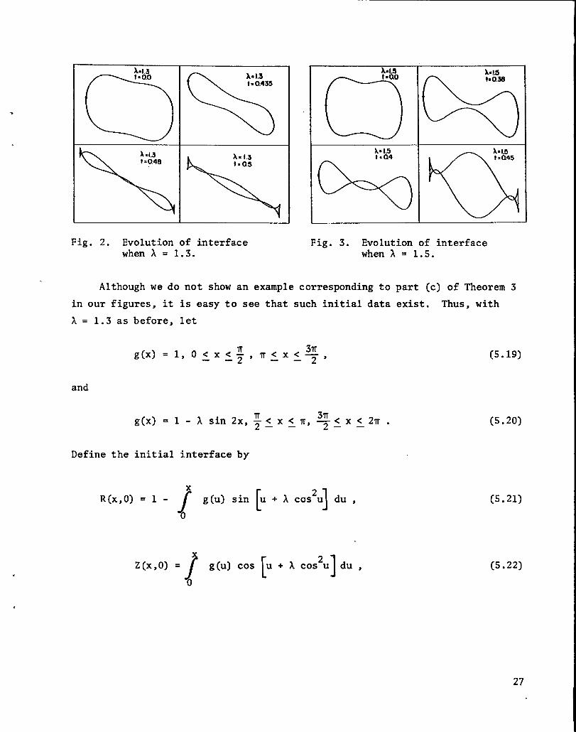
With A = 1.3,the smoothinitialcurvedevelopstwo singularpoints,at

x = 3n/4 and x = 7m/4,as t + T = 0.4350 This case correspondsto part (b)c

of Theorem3. The evolutionof the interfaceis shownin Fig. 2. Figures

2 and 3 were reproducedfrom computerplotswherethe scaleson the vertical

and horizontalaxes are automaticallyadjusted,so that the resultingcurve

nearlyfillsthe frame. In our case,this adjustmentleadsto a vertical

magnificationwhich greatlyexceedsthe horizontalmagnification.The point

x = 3r/4 in Figs.2 and 3 is markedby a smallsquare. At t = Tc = 0.435,

we see that the curvatureat x = 3n/4appearsrathermodestin Fig. 2. We

assurethe readerthat this is a consequenceof the automaticscaling. The

curvatureat that point is infinite,althoughthe tangentthereturns con-

tinuously. The two cuspsnear x = 3n/4 are clearlyvisiblein Fig. 2, for

t > Tc, as well as the appearanceof multiplepoints.

It is possiblefor multiplepointsto appearbeforet = Tc. ThUS with

A = 1.5, the bottompart of the curve (nearx = 5n/4)smoothlyinterlaces

the top part (nearx = m/4) at a valueof t < Tc = 0.4, as shownin Fig. 3.

This experimentconfirmsthe fact thatTc is reallyan upperbound on the

time duringwhich the model is valid. In a realplasma,shock-shockinter-

actionwouldhave spoiledthe modelwell beforesuch an interlacingcould

occur.

26

,

.

,

A=I.3

o

t=0.0

\

X.1.3t=0.48 k=1.3

\

t80.5

Fig. 2. Evolutionof interfacewhen A = 1.3.

A.I.5t .00

c—

A*I5

%

ho.3s

X91.5

Q

t za45

Fig. 3. Evolutionof interfacewhen A = 1.5.

Althoughwe do not showan examplecorrespondingto part (c)of Theorem3

in our figures,it is easyto see that such initialdata exist. Thus,with

A= 1.3 as before,let

g (x)=1, o<x~; 3?T— , r~x < — ,

–2

and

g(x) = 1 - A sin 2x, ~<x<2T.;< x< ‘lrJ _ _——

Define the initial interface

R(x,O)=x

1-f

g (u)

o

by

3in[ 1U + ~ COS2U du ,

Z(x,o) = J [ 1g(u) COS U + ~ COS2U du ,

0

(5.19)

(5.20)

(5.21)

(5.22)

27

0CXC27T , so that,——

e(x)= 2x+~cosxo

Let M(x,O) s O and let

U(x,O) = - cos f3(x), V(X, O) = - sin e(x).

It can be shownthat the initialinterfaceis a simpleclosedcurvewith

continuouslyturningtangent. We have g(x) > 1 on [0,2m],Tc = 1, and—g(x) - Tcex(x)= O on [IT/2,1T]and [31T/2,21T].Accordingly,the interface

(5.23)

(5.24)

a

developscornersat t = 1, with the polaranglemakinga jump of (A + n/2)

rad at thesepoints.

REFERENCES

1. M. Rosenbluth,“InfiniteConductivityTheoryof the Pinch,”Los AlamosScientificLaboratoryreportLA-1850(March1955).

2. H, M. Nelson,K. H. Brown,and C. A. Hart,“ComputerModelof A FastToroidalPlasmaCompression,with Applicationto the Topolotron,”Phys.Fluids 19, 1810-1819(1976).

,

.

,

3. R. D. Richtmyerand K. W. Morton,DifferenceMethodsfor InitialValueProblems, 2nd Ed. (Wiley-Interscience,New York, 1967) p. 59.

28