Long-Term Growth and Persistence with

Endogenous Depreciation: Theory and Evidence∗

Ilaski Barañanoa , Diego Romero-Ávilab

aUniversity of the Basque Country, Depart. Fundamentos del Análisis Económico I, Bilbao, Spain.

bPablo de Olavide University, Depart. Economía, Métodos Cuantitativos e Historia Económica,

Sevilla, Spain.

Abstract

Previous research has shown a strong positive correlation between short-term

persistence and long-term output growth as well as between depreciation rates

and long-term output growth. This evidence, therefore, contradicts the standard

predictions from traditional neoclassical or AK-type growth models with exogenous

depreciation. In this paper, we first confirm these findings for a larger sample of

101 countries. We then study the dynamics of growth and persistence in a model

where both the depreciation rate and growth are endogenous and procyclical. We

find that the model’s predictions become consistent with the empirical evidence on

persistence, long-term growth and depreciation rates.

∗We thank Jesús Crespo-Cuaresma, Peter Egger, Luca Gambetti, Miguel León-Ledesma, Lilia

Maliar, Serguei Maliar, Ignacio Palacios-Huerta and Luis Puch for valuable comments and suggestions.

Ilaski Barañano acknowledges financial support from the Spanish Ministry of Science and Techno-

logy through grant ECO2009-07939 and Departamento de Educación, Universidades e Investigación

del Gobierno Vasco (IT-223-07). Diego Romero-Ávila acknowledges financial support from the Spanish

Ministry of Science and Technology through grant ECO2009-13357 and from the Andalusian Council of

Innovation and Science under grant number SEJ-4546. Corresponding author: Depart. Fundamentos

del Análisis Económico I, University of the Basque Country, Lehendakari Agirre Etorbidea 83, 48015

Bilbao, Spain. Tel.: +34 94 601 3822; Fax: +34 94 601 3891. E-mail: ilaski.baranano@ehu.es.

1

Keywords: Real Business Cycle Models; Endogenous Growth; Stochastic

Trends; Persistence; Capital Utilization; Dynamic Panel Data Models.

JEL classification: C22; C23; E32; O40.

2

1 Introduction

Empirical evidence on the persistence of output fluctuations shows large differences

across countries. Using quarterly GNP data for the Group of Seven (G7) countries,

Campbell and Mankiw (1989) find important differences in the estimates of persis-

tence. Consistent with this evidence, Cogley (1990) reports significant differences in

the variability of the permanent component of output in a similar sample of countries.

Further, Fatás (2000) finds that there is a positive and significant correlation between

the degree of persistence of short-term fluctuations and long-term average growth rates

for a sample of countries that includes the G7 countries and eight additional OECD

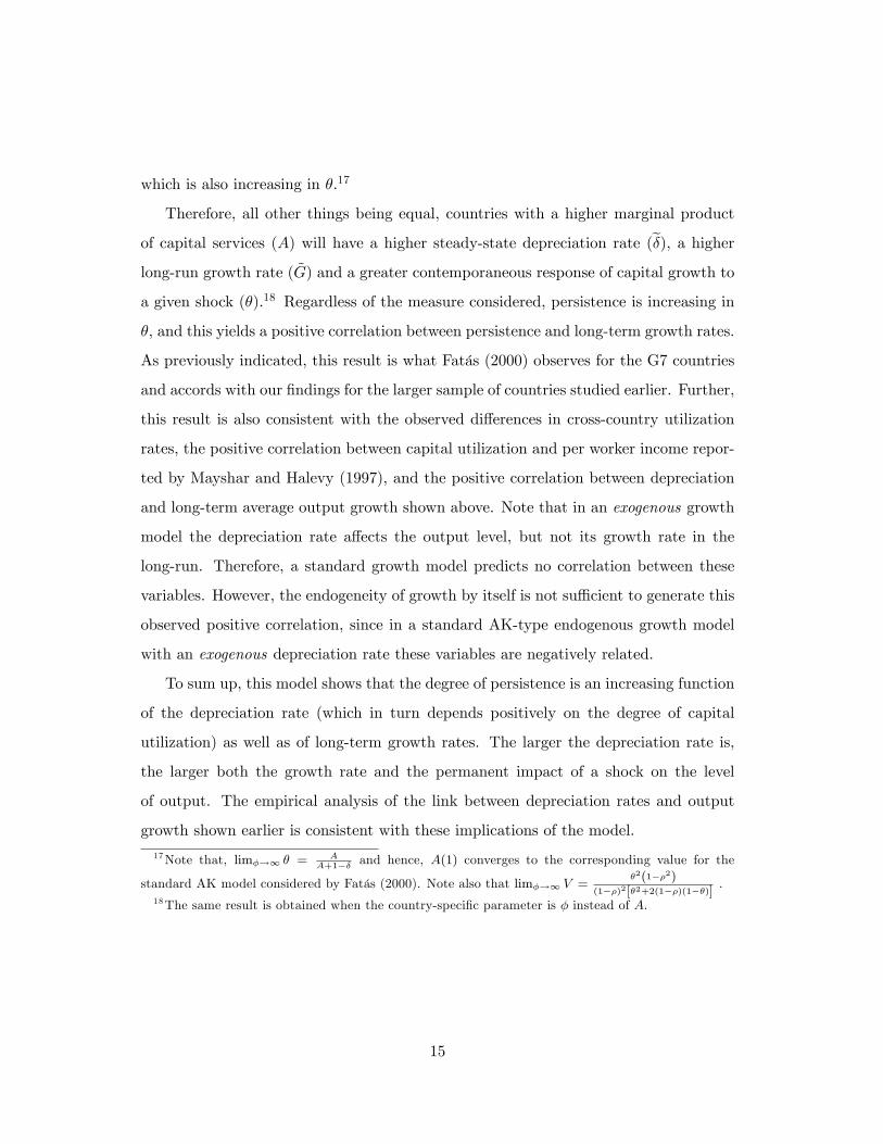
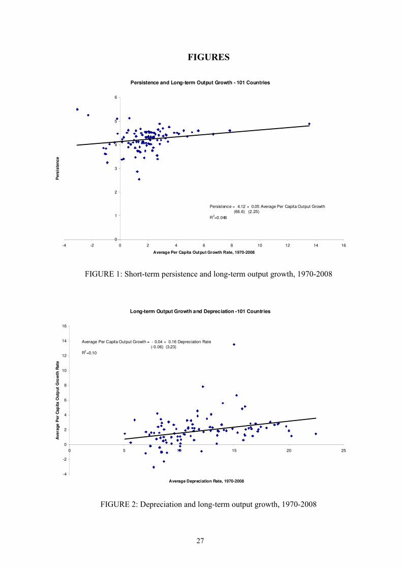
countries. Figure 1 extends the results by Fatás (2000) for the G7 countries by plotting

the degree of persistence of the GDP series against long-term average per capita output

growth for a broad sample of 101 countries over the period 1970-2008.1

[Insert Figure 1 about here]

The degree of persistence is computed using Cochrane (1988)’s variance ratio with

a window of five years. To construct it, we employ heteroskedasticity robust standard

errors and correct for small-sample bias in the variance following the procedure outlined

in Campbell, Lo and Mackinley (1997). The variance ratio is a measure of the extent to

which annual fluctuations are trend reverting and, in turn, a measure of the permanent

impact of business cycles on trend output. As shown in Figure 1, there is a clear positive

correlation between the persistence of output fluctuations and long-term output growth.

The cross-section regression provides evidence of a statistically significant (at the 1%

level) positive coeffi cient on long-term average growth. This indicates that the greater

the growth rate of an economy, the larger the permanent effect of cyclical fluctuations

on trend output.

In standard RBC models cyclical fluctuations are simply deviations around an exo-

genous trend driven by the state of technological progress. In these models, there is1The annual real GDP series employed throughout the paper are expressed in constant 2000 US$

and were retrieved from the World Development Indicators of the World Bank (2010).

1

no correlation between persistence and long-term output growth.2 As noted by Fatás

(2000), however, the significantly positive correlation between short-term persistence

and long-run growth is consistent with RBC models with endogenous productivity

shocks. In these models the degree of short-term persistence captures the extent to

which cyclical fluctuations affect technological progress, which endogenously determ-

ines long-term growth.3 Using a standard AK model, Fatás shows that a positive cor-

relation between persistence and growth can be obtained when the stochastic nature

of the trend is endogenous.

The standard AK growth model considers the rate of depreciation as a constant and

assumes that capital services are a fixed proportion of the existing capital stock, as is

usual in the growth literature. In this setting, the marginal cost of capital utilization

is zero, which implies an optimal capital utilization rate equal to one. The empirical

evidence on depreciation and capital utilization rates, however, is not consistent with

this assumption.4 In fact, the empirical evidence on depreciation and capital utilization

rates across countries documents: (i) large differences in cross-country utilization rates,

(ii) a positive correlation between capital utilization and per capita income, and (iii) a

positive correlation between the depreciation and long-term average per capita income

growth rates.5

2This is because all GDP series would be characterized by a random walk with a drift, which would

render a variance ratio equal to one for all countries in the sample.3Provided that the amount of resources allocated to growth varies procyclically, temporary shocks

produce permanent effects on output.4Using aggregate US manufacturing data, Epstein and Denny (1980) and Kollintzas and Choi (1985)

provide evidence against the standard assumption of a constant depreciation rate. Abadir and Talmain

(2001) estimate time-varying depreciation rates for Canada, Germany, Japan and the UK. In addition,

Foss (1981), Orr (1989) and Beaulie and Mattey (1998) find upward trends for the capital utilization

rate in the US.5Using data for Pakistan, South Corea and the US, Kim and Watson (1974) find that the rate of

capital utilization increases with per capita income. The same result is found by Mayshar and Halevy

(1997) for a sample of 24,000 companies in ten European countries. Anxo et al. (1995) provide evidence

of a large variation in utilization rates across Europe as well as much higher utilization rates in US

manufacturing industries than in Europe. Finally, using cross-sectional data of 85 countries from the

2

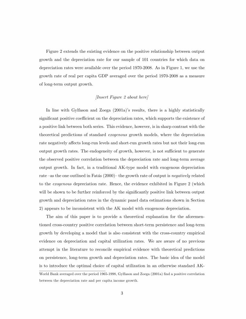
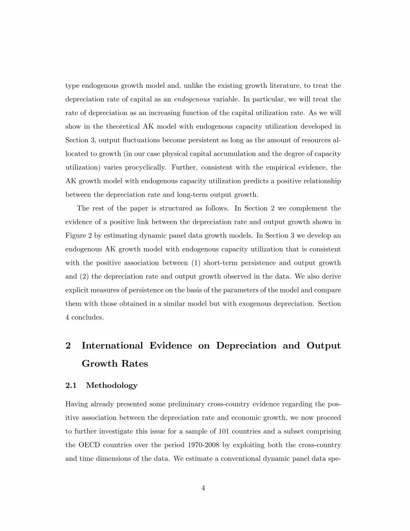
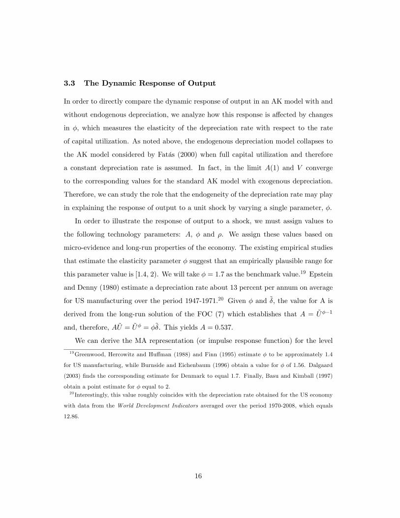
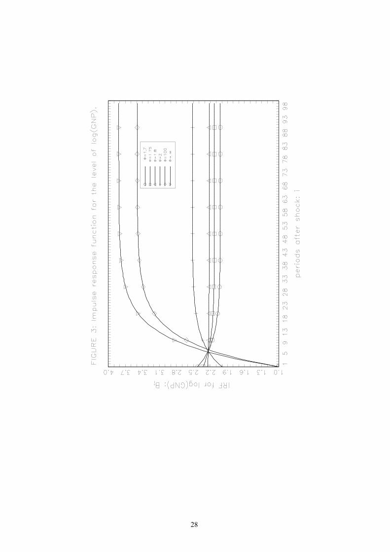
Figure 2 extends the existing evidence on the positive relationship between output

growth and the depreciation rate for our sample of 101 countries for which data on

depreciation rates were available over the period 1970-2008. As in Figure 1, we use the

growth rate of real per capita GDP averaged over the period 1970-2008 as a measure

of long-term output growth.

[Insert Figure 2 about here]

In line with Gylfason and Zoega (2001a)’s results, there is a highly statistically

significant positive coeffi cient on the depreciation rates, which supports the existence of

a positive link between both series. This evidence, however, is in sharp contrast with the

theoretical predictions of standard exogenous growth models, where the depreciation

rate negatively affects long-run levels and short-run growth rates but not their long-run

output growth rates. The endogeneity of growth, however, is not suffi cient to generate

the observed positive correlation between the depreciation rate and long-term average

output growth. In fact, in a traditional AK-type model with exogenous depreciation

rate —as the one outlined in Fatás (2000)—the growth rate of output is negatively related

to the exogenous depreciation rate. Hence, the evidence exhibited in Figure 2 (which

will be shown to be further reinforced by the significantly positive link between output

growth and depreciation rates in the dynamic panel data estimations shown in Section

2) appears to be inconsistent with the AK model with exogenous depreciation.

The aim of this paper is to provide a theoretical explanation for the aforemen-

tioned cross-country positive correlation between short-term persistence and long-term

growth by developing a model that is also consistent with the cross-country empirical

evidence on depreciation and capital utilization rates. We are aware of no previous

attempt in the literature to reconcile empirical evidence with theoretical predictions

on persistence, long-term growth and depreciation rates. The basic idea of the model

is to introduce the optimal choice of capital utilization in an otherwise standard AK-

World Bank averaged over the period 1965-1998, Gylfason and Zoega (2001a) find a positive correlation

between the depreciation rate and per capita income growth.

3

type endogenous growth model and, unlike the existing growth literature, to treat the

depreciation rate of capital as an endogenous variable. In particular, we will treat the

rate of depreciation as an increasing function of the capital utilization rate. As we will

show in the theoretical AK model with endogenous capacity utilization developed in

Section 3, output fluctuations become persistent as long as the amount of resources al-

located to growth (in our case physical capital accumulation and the degree of capacity

utilization) varies procyclically. Further, consistent with the empirical evidence, the

AK growth model with endogenous capacity utilization predicts a positive relationship

between the depreciation rate and long-term output growth.

The rest of the paper is structured as follows. In Section 2 we complement the

evidence of a positive link between the depreciation rate and output growth shown in

Figure 2 by estimating dynamic panel data growth models. In Section 3 we develop an

endogenous AK growth model with endogenous capacity utilization that is consistent

with the positive association between (1) short-term persistence and output growth

and (2) the depreciation rate and output growth observed in the data. We also derive

explicit measures of persistence on the basis of the parameters of the model and compare

them with those obtained in a similar model but with exogenous depreciation. Section

4 concludes.

2 International Evidence on Depreciation and Output

Growth Rates

2.1 Methodology

Having already presented some preliminary cross-country evidence regarding the pos-

itive association between the depreciation rate and economic growth, we now proceed

to further investigate this issue for a sample of 101 countries and a subset comprising

the OECD countries over the period 1970-2008 by exploiting both the cross-country

and time dimensions of the data. We estimate a conventional dynamic panel data spe-

4

cification that regresses real per capita output growth on its main growth determinants

according to standard growth theory:

yi,t − yi,t−1 = γyi,t−1 + η′Xi,t + αi + δt + εi,t (1)

where y is the logarithm of real per capita GDP, αi is a set of unobserved country-

specific effects (to account for time-invariant country-specific structural characteristics)

and δt is a set of time-specific effects (to account for common shocks affecting all coun-

tries in a given year). X represents a set of explanatory variables that includes the

population growth rate (to capture the growth reduction in per capita terms due to

increases in population), the secondary school enrollment rate (as a measure of human

capital accumulation), trade size (computed as the ratio of exports plus imports to

GDP), the agricultural share of GDP (to account for the negative effects of natural re-

source abundance due to induced rent-seeking and the Dutch disease),6 and a variable

accounting for the accumulation of physical capital. Unlike most previous studies, the

share of gross domestic fixed capital formation over GDP is split into the share of net

investment over GDP plus the depreciation rate.7 The depreciation of fixed capital —

measured as a proportion of GDP—represents the consumption of fixed capital as given

by the replacement value of capital used up in the production process.8 Finally, lagged

6See Gylfason and Zoega (2001b) for more details on these mechanisms.7To the best of our knowledge, the only exception is Gylfason and Zoega (2001a) who estimate a

similar specification to ours but using cross-sectional data averaged over the period 1965-1998 for a

sample of 85 countries rather than panel data.8The depreciation rates are World Bank staff estimates using data from the United Nations Statistics

Division’s National Accounts Statistics. According to the System of National Accounts (see United

Nations, 2009), the formal definition of consumption of fixed capital is the decline, during the course of

the accounting period, in the current value of the stock of fixed assets owned and used by a producer

as a result of physical deterioration, normal obsolescence or normal accidental damage. It is important

to stress the fact that the value of the assets not only declines because of physical deterioration but

also due to the decrease in the demand for their services as a result of technological progress and

the appearance of new substitutes for them (i.e. obsolescence). However, this variable only considers

normal, expected rates of obsolescence, not unexpected ones. As with total output or intermediate

5

output (yi,t−1) accounts for convergence dynamics of per capita output. The depreci-

ation rate along with the other variables were retrieved from the World Development

Indicators of the World Bank (2010).

Traditionally, this specification has been estimated via the Least Squares Dummy

Variables (LSDV) estimator. This estimator, however, is unable to correct for the

simultaneity bias due to the endogeneity of many of the regressors as well as for the

omitted variable bias and the bias caused by the correlation of the lagged dependent

variable and αi. To deal with these shortcomings, Arellano and Bond (1991) propose to

use the Generalized Method of Moments (GMM) instrumental variables dynamic panel

data estimator called difference estimator. They difference equation (1):

(yi,t − yi,t−1)− (yi,t−1 − yi,t−2) = γ(yi,t−1 − yi,t−2) + η′(Xi,t −Xi,t−1) +

+(δt − δt−1) + (εi,t − εi,t−1) (2)

While differencing eliminates the Nickel (1981) bias caused by the correlation

between lagged output and country-specific effects, it introduces a new bias caused

by the correlation of the new error term (εi,t − εi,t−1) with the lagged dependent vari-

able (yi,t−1−yi,t−2). The difference estimator uses previous realizations of the regressors

to instrument for their current values in the first-differenced specification. Under the

assumption of no serial correlation in the error term and the weak exogeneity of the

regressors, Arellano and Bond (1991) propose to employ the following conditions:

E [yi,t−s(εi,t − εi,t−1)] = 0 for s ≥ 3; t = 4, ..., T, (3)

E [Xi,t−s(εi,t − εi,t−1)] = 0 for s ≥ 2; t = 3, ..., T, (4)

Arellano and Bover (1995) and Blundell and Bond (1998) show that in the case

of persistent regressors, lagged levels of the variables are weak instruments for the

consumption, consumption of fixed capital is calculated using current prices or rentals of fixed assets

instead of employing historic costs as in business accounting. See more details in United Nations (2009)

and OECD (2009).

6

first-differenced regressors. This leads to a fall in precision as well as to biased coeffi -

cients. To overcome these shortcomings, Arellano and Bover (1995) and Blundell and

Bond (1998) suggest the use of the system estimator that utilizes instruments in levels

and first-differences to improve effi ciency.9 The instruments for the first-differenced

specification are the same as above. The instruments for the regression in levels are

the lagged differences of the variables. In order to avoid using redundant instruments

in first-differences that could lead to overfitting bias, we only employ the following

additional moment conditions for the regression in levels:

E [(yi,t−s − yi,t−s−1)(αi + εi,t)] = 0 for s = 1; (5)

E [(Xi,t−s −Xi,t−s−1)(αi + εi,t)] = 0 for s = 1; (6)

A further concern in the use of the system GMM estimator is the downward bias as-

sociated with the standard errors of the estimates, particularly when the cross-sectional

dimension is relatively small, which in turn may lead to spuriously significant regressors.

To overcome this diffi culty, we use the one-step estimator since the asymptotic standard

errors for the two-step estimator are biased downwards. As a result, the asymptotic

inference from the one-step standard errors are more reliable. In addition, we apply

the small-size correction factors proposed by Windmeijer (2005).

The consistency of the system estimator depends on the validity of the instruments

and the absence of serial correlation of second-order in the first-differenced error term.

Therefore, we test these assumptions using the Sargan test for over-identifying restric-

tions and the test for second-order autocorrelation proposed by Arellano and Bond

(1991). Failing to reject the null hypotheses of overall validity of the instruments and

absence of second-order serial correlation in the first-differenced error for the respective

tests would give support to an endogenous growth model with endogenous depreciation.

9More recently, Hauk and Wacziarg (2009) have shown that the system estimator appears to out-

perform the difference estimator in terms of the biases emerging from the presence of measurement

error in growth regressions.

7

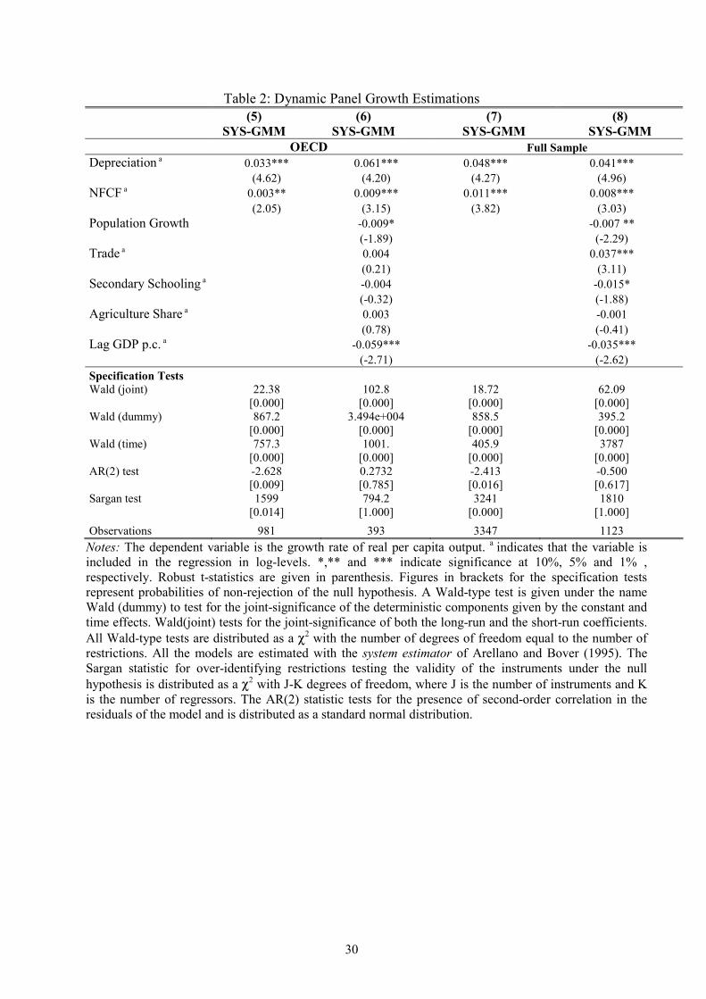
2.2 Empirical Findings

Before presenting the estimates obtained with the system estimator that corrects for

endogeneity bias, the Nickel bias and omitted variable bias, Table 1 reports the results

from the application of the LSDV estimator. The basic specification only includes as

stochastic regressors the depreciation rate and net fixed capital formation over GDP,

while the augmented specification further adds lagged output and four other additional

variables such as population growth, the trade share of GDP, the secondary school

enrollment rate and the agricultural share of GDP. We present the results for the

OECD sample as well as for the full sample comprising 101 countries.10

[Insert Table 1 about here]

Interestingly, model (1) shows that there is a highly statistically significant coeffi -

cients on the depreciation rate and the net investment rate for the basic specification

in the OECD sample. The regression coeffi cient on the depreciation rate capturing

replacement investment is about ten times greater than the coeffi cient associated with

net investment. Model (2) also yields a statistically significant coeffi cient on replace-

ment investment which is substantially greater (about sevenfold) than the coeffi cient

on net investment. This augmented specification also renders, as expected, a statist-

ically significant negative coeffi cient on lagged output and population growth, while

the coeffi cient on the trade share, secondary schooling and the agricultural share are

statistically insignificant. The Wald statistics support the significance of country and

time fixed effects.

The results for the full sample also support the statistical significance of the pos-

itive coeffi cient on replacement investment and net investment for both the basic and

augmented specifications. In this case, the coeffi cient on depreciation appears to be

between four and five times greater than that on net investment.

10Table A1 in Appendix A reports the identity of the countries in the sample and some descriptive

statistics of the relevant variables.

8

This basic finding appears to contradict the standard predictions from traditional

neoclassical or AK-type endogenous growth models with exogenous depreciation. For

exogenous growth models the depreciation rate would only negatively affect transitional

growth, while for AK models with exogenous depreciation it would exert a negative

effect on long-run growth. As will be shown in Section 3, a positive link between the

depreciation rate and long-term output growth appears more in line with the predictions

of the AK model with endogenous depreciation.

Table 2 presents the results from the system GMM estimator. We find that the

statistical significance, sign and size of the coeffi cients on replacement investment and

net investment are very similar to those obtained with the LSDV estimator. Again,

the size of the coeffi cient on the depreciation rate more than quadruples the size of

the coeffi cient on the net investment rate. Interestingly, we reject the null hypotheses

of overall validity of instruments and absence of second-order serial correlation with

the Sargan and AR(2) tests for the basic specification with only depreciation and net

investment. In contrast, when we add lagged per capita output and the rest of explan-

atory variables we fail to reject both null hypotheses, thereby supporting the validity

of the augmented specification.

[Insert Table 2 about here]

Overall, the results in this section show that both the depreciation rate and per

capita output growth appear to be positively correlated. The statistical and economic

significance of the coeffi cients on the depreciation rate appear to be quite robust to

changes in the sample of countries as well as in the set of explanatory variables. In-

terestingly, the size of the coeffi cient on replacement investment is much higher than

that on net investment. Hence, these results indicate that traditional exogenous and

endogenous growth theory (of the AK type) for which the depreciation rate affects

negatively either transitional growth or long-run growth, may be neglecting some im-

portant features of the dynamics of growth. A natural candidate would be to consider

an endogenous depreciation rate that directly depends on capacity utilization, which in

9

turn varies procyclically with the state of the cycle. This feature is introduced in the

AK model with endogenous capacity utilization presented in the next section.

3 The Setup of the Model

The framework is a simplified, stochastic version of Chatterjee’s (2005) endogenous

growth model: an AK-type growth model augmented by endogenous capital utilization.

We consider this endogenous growth model because of its simplicity.

Consider a closed economy without a public sector. The economy is populated by a

continuum of identical, infinitely lived agents which derive utility from the consumption

of a final good and discount future utility at a rate β ∈ (0, 1). Preferences are given

by∑∞

t=0 βt C

1−σt −11−σ , where Ct denotes consumption. We assume that the labor supply

is inelastic and we normalize it to unity.

The technology of the consumption good is described by the aggregate production

function Yt = AZtUtKt, where A is a scale parameter, UtKt is the flow of capital services

derived from the available capital stock, Yt denotes the corresponding flow of output,

and Zt is a temporary exogenous shock that captures the state of the technology. As

suggested by Taubman and Wilkinson (1970) and Calvo (1975), and following Chatter-

jee (2005), we define the rate of capital utilization Ut as the intensity (measured in hours

per week) with which the available capital stock is used. In this way, firms are provided

by an extra margin to vary output, namely the intensive margin. The productivity

shock Zt is assumed to follow the autoregressive process: zt+1 = ρzt+εt+1, 0 < ρ < 1,

where lower case letters represent logarithms, a circumflex on top of the variable denotes

deviations from its steady state value and εt is a white noise.

In a closed economy without public sector all output is devoted to consumption

or gross investment. Hence, the resource constraint of the economy is Ct + It = Yt.

The capital stock evolves according to Kt+1 = Kt(1 − δt) + It. Following Greenwood,

Hercowitz and Huffman (1988), we also assume that the rate of depreciation of the

capital stock is a convex, constant elasticity function of its rate of utilization: δ(Ut) =

10

1φUt

φ, where φ > 1 and 0 ≤ δ(Ut) ≤ 1. Note that, in contrast to the usual assumption

in the growth literature, the marginal depreciation cost of capital utilization δ′(Ut) is

variable. The parameter φ measures the elasticity of the depreciation rate with respect

to the rate of capital utilization.11 As is already known, due to the sensitivity of the

depreciation rate of capital to the choice of capital utilization, it may not be optimal to

fully utilize the capital. Obviously, this model collapses to the AK model considered by

Fatás (2000) when full capital utilization, and therefore a constant depreciation rate,

is assumed.

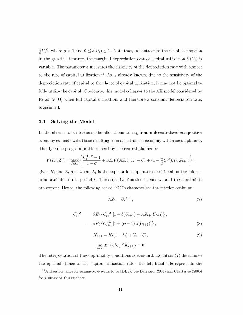
3.1 Solving the Model

In the absence of distortions, the allocations arising from a decentralized competitive

economy coincide with those resulting from a centralized economy with a social planner.

The dynamic program problem faced by the central planner is:

V (Kt, Zt) = maxCt,Ut

{C1−σt − 1

1− σ + βEtV (AZtUtKt − Ct + (1− 1

φUtφ)Kt, Zt+1)

},

given Kt and Zt and where Et is the expectations operator conditional on the inform-

ation available up to period t. The objective function is concave and the constraints

are convex. Hence, the following set of FOC’s characterizes the interior optimum:

AZt = Utφ−1, (7)

C−σt = βEt{C−σt+1 [1− δ(Ut+1) +AZt+1Ut+1]

},

= βEt{C−σt+1 [1 + (φ− 1) δ(Ut+1)]

}, (8)

Kt+1 = Kt(1− δt) + Yt − Ct, (9)

limt→∞

Et{βtC−σt Kt+1

}= 0.

The interpretation of these optimality conditions is standard. Equation (7) determines

the optimal choice of the capital utilization rate: the left hand-side represents the11A plausible range for parameter φ seems to be [1.4, 2). See Dalgaard (2003) and Chatterjee (2005)

for a survey on this evidence.

11

marginal benefit of capital utilization and the right hand-side the marginal cost of

capital utilization. Hence, in this setting, it is optimal to utilize capital less than fully,

i.e. Ut ∈ (0, 1).12

In the long-run equilibrium, output, consumption and capital will grow at a common

rate (G) and therefore there are no steady state levels for these variables. Let YtKt

and CtKt

be the stationary variables for which we obtain the following steady state

equilibrium: U = (A)1

φ−1 , YtKt

= AU, δ = 1φYtKt, G =

{β[1 + (φ− 1) δ

]} 1σ, and Ct

Kt=

(φ− 1) δ + 1− G.

Let St be the proportion of income that is not consumed: Ct = (1 − St)Yt. In

steady state the saving rate is given by S = G−(1−δ)A . Hence, the long-run solution to

this model is characterized by a constant saving rate, a constant but not full capital

utilization rate, and a balanced growth path with output, consumption and capital

growing at the same rate. These constant levels depend on the marginal product of

capital services, A, and the elasticity of the depreciation rate with respect to the capital

utilization rate, φ. Assume now that A is a country-specific technological parameter.

Countries with a higher A will then have both a greater U and therefore a greater δ.

From the FOC (8) it is easy to verify that countries with a higher A will also have a

greater long-run gross growth rate (G).

We rewrite the equilibrium dynamics of the model in terms of the saving rate, St.

Combining conditions (7) and (8) and taking into account from the resource constraint

(9) that Kt+1

Kt= 1− 1

φ (AZt)φφ−1 (1− φSt), the following expression is obtained:1− 1

φ(AZt)φφ−1 (1− φSt)

(1− St)(AZt)φφ−1

σ = βEt

1 + 1φ(AZt+1)

φφ−1 (φ− 1)[

(1− St+1)(AZt+1)φφ−1

]σ . (10)

Since there is no closed-form solution to the equilibrium, we approximate it by linear-

izing both equations around the steady state values. From (10) we obtain the following

12This is in contrast to the existing growth literature which assumes a constant depreciation rate,

implying a zero marginal cost of capital utilization and hence being optimal to fully utilize capital. As

shown by Chatterjee (2005), there exists an optimal Ut ∈ (0, 1), under the mild condition A < 1.

12

first order stochastic difference equation:

a1st + a2zt = a3Et (st+1) + a4Et (zt+1) ,

where all a i are functions of the parameters of the model and xt denotes the deviation

of variable Xt from its steady state value in logarithms.13 Since zt = ρzt−1 + εt, the

solution is given by:

st = azt, where a =ρa4 − a2

a1 − ρa3. (11)

By linearizing the resource constraint around the steady state and by substituting the

solution given by (11), we obtain the following expression for the deviations of capital

growth from its steady state value G:

∆kt+1 = θzt, where θ = Aφφ−1

aS + S φφ−1 −

1φ−1

G,

where θ captures the contemporaneous impact of shocks on physical capital accumu-

lation. Therefore, shocks have an effect on capital accumulation and growth varies

procyclically. Plugging this expression into the production function and taking into

account from (7) that ut = 1φ−1 zt, the deviations of output growth from its steady

state value are given by the following moving average representation:

∆yt = A(L)εt =

[φφ−1 −

(φφ−1 − θ

)L]

1− ρL εt, (12)

where A(L) is an infinite polynomial in the lag operator.

3.2 Persistence Results

This endogenous growth model has some important properties for growth and fluctu-

ations. The model generates integrated time series, even though the underlying shocks

are stationary. After the effects of these shocks vanish, output does not return to its

trend level. That is, temporary shocks have permanent effects on output since they

generate endogenous responses in the amount of resources allocated to growth. As a

13Appendix B provides the mapping between these parameters and the deep parameters of the model.

13

result, growth dynamics is an important component of the propagation mechanism in

which the stochastic properties of the trend are endogenous. As argued by Fatás (2000),

in this setting, output persistence is not simply equal to the persistence of disturbances

since shocks endogenously generate changes in the capital accumulation rate that result

in persistent responses of output.14

The permanent impact of a shock on the level of output equals the infinite sum

of the moving average coeffi cients, which is A(1).15 For simplicity and to facilitate

comparison with the results obtained by Fatás (2000), we also restrict our attention to

σ = 1 in which case the utility function is logarithmic.16 In the model under study the

measure of persistence A(1) is given by:

A(1) =θ

1− ρ, where θ =A

φφ−1

1 +(

1− 1φ

)A

φφ−1

=φ

φ− 1(1− β

G), (13)

which is increasing in the parameter θ that represents the contemporaneous impact that

shocks exert on the accumulation of physical capital. Hence, the greater the growth

rate, the greater the effects of shocks on the output level through a higher response of

capital accumulation to the shock.

Cochrane (1988) suggests another measure of persistence: the weighted sum of

autocorrelations V = limJ→∞[1 + 2

∑Jj=1(1− j

J+1)ψj

], where ψj is the jth autocor-

relation of the growth rate of output. In the model under study, V is given by:

V =

(1− ρ2

)θ2

(1− ρ)2

[(φφ−1

)2− 2ρ( φ

φ−1)(

φφ−1 − θ

)+(

φφ−1 − θ

)2] , (14)

14A standard RBC model would predict no correlation between persistence and growth as growth

would be treated as exogenous.15 In Appendix C we provide the derivation of the expressions linking this persistence measure and

the variance ratio (V ) with the θ parameter.16When the standard AK model is considered, there is no closed-form solution to the equilibrium

even for σ = 1. However, when the endogenous depreciation AK model is considered and σ = 1, there

exists a closed-form solution to the equilibrium. Obviously, by using this closed-form solution we would

obtain the same equation (12), with no need to calculate a. This is proven in Appendix B.

14

which is also increasing in θ.17

Therefore, all other things being equal, countries with a higher marginal product

of capital services (A) will have a higher steady-state depreciation rate (δ), a higher

long-run growth rate (G) and a greater contemporaneous response of capital growth to

a given shock (θ).18 Regardless of the measure considered, persistence is increasing in

θ, and this yields a positive correlation between persistence and long-term growth rates.

As previously indicated, this result is what Fatás (2000) observes for the G7 countries

and accords with our findings for the larger sample of countries studied earlier. Further,

this result is also consistent with the observed differences in cross-country utilization

rates, the positive correlation between capital utilization and per worker income repor-

ted by Mayshar and Halevy (1997), and the positive correlation between depreciation

and long-term average output growth shown above. Note that in an exogenous growth

model the depreciation rate affects the output level, but not its growth rate in the

long-run. Therefore, a standard growth model predicts no correlation between these

variables. However, the endogeneity of growth by itself is not suffi cient to generate this

observed positive correlation, since in a standard AK-type endogenous growth model

with an exogenous depreciation rate these variables are negatively related.

To sum up, this model shows that the degree of persistence is an increasing function

of the depreciation rate (which in turn depends positively on the degree of capital

utilization) as well as of long-term growth rates. The larger the depreciation rate is,

the larger both the growth rate and the permanent impact of a shock on the level

of output. The empirical analysis of the link between depreciation rates and output

growth shown earlier is consistent with these implications of the model.

17Note that, limφ→∞ θ = AA+1−δ and hence, A(1) converges to the corresponding value for the

standard AK model considered by Fatás (2000). Note also that limφ→∞ V =θ2(1−ρ2)

(1−ρ)2[θ2+2(1−ρ)(1−θ)].

18The same result is obtained when the country-specific parameter is φ instead of A.

15

3.3 The Dynamic Response of Output

In order to directly compare the dynamic response of output in an AK model with and

without endogenous depreciation, we analyze how this response is affected by changes

in φ, which measures the elasticity of the depreciation rate with respect to the rate

of capital utilization. As noted above, the endogenous depreciation model collapses to

the AK model considered by Fatás (2000) when full capital utilization and therefore

a constant depreciation rate is assumed. In fact, in the limit A(1) and V converge

to the corresponding values for the standard AK model with exogenous depreciation.

Therefore, we can study the role that the endogeneity of the depreciation rate may play

in explaining the response of output to a unit shock by varying a single parameter, φ.

In order to illustrate the response of output to a shock, we must assign values to

the following technology parameters: A, φ and ρ. We assign these values based on

micro-evidence and long-run properties of the economy. The existing empirical studies

that estimate the elasticity parameter φ suggest that an empirically plausible range for

this parameter value is [1.4, 2). We will take φ = 1.7 as the benchmark value.19 Epstein

and Denny (1980) estimate a depreciation rate about 13 percent per annum on average

for US manufacturing over the period 1947-1971.20 Given φ and δ, the value for A is

derived from the long-run solution of the FOC (7) which establishes that A = Uφ−1

and, therefore, AU = Uφ = φδ. This yields A = 0.537.

We can derive the MA representation (or impulse response function) for the level

19Greenwood, Hercowitz and Huffman (1988) and Finn (1995) estimate φ to be approximately 1.4

for US manufacturing, while Burnside and Eichenbaum (1996) obtain a value for φ of 1.56. Dalgaard

(2003) finds the corresponding estimate for Denmark to equal 1.7. Finally, Basu and Kimball (1997)

obtain a point estimate for φ equal to 2.20 Interestingly, this value roughly coincides with the depreciation rate obtained for the US economy

with data from the World Development Indicators averaged over the period 1970-2008, which equals

12.86.

16

of log GNP by rewriting equation (12):

yt = yt−1 + lnG+A(L)εt

= y0 + t lnG+B(L)εt

where Bi =∑i

j=0Aj . Therefore, the limit of Bi is A(1), which measures the response

of yt+i to a shock at time t for a large i.21

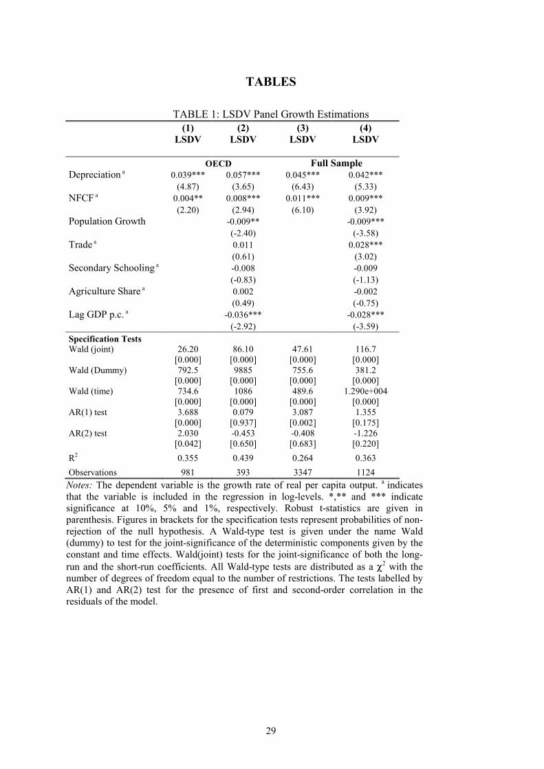
Figure 3 illustrates the impulse response functions for the endogenous depreciation

model with different values of φ. We calculate these responses by setting ρ = 0.9.

This figure shows that as the elasticity of depreciation with respect to the rate of

capital utilization φ increases, the permanent effect of a shock on output increases. In

Appendix D we prove that A(1) increases with φ.

[Insert Figure 3 about here]

As mentioned above, if the depreciation rate were treated as exogenous, A(1) would

converge to the corresponding value of the standard AK model in Fatás (2000), i.e.

limφ→∞A(1) = AA+1−δ

11−ρ and, hence, this model would overstate the long-run impact

of a shock on the level of output.22 The logic behind this result is the following. Tem-

porary shocks become persistent in both models as they have an effect on the amount

of resources allocated to capital accumulation. However, when the depreciation rate is

endogenous, temporary shocks affect capital accumulation through two channels: the

marginal product of capital and the depreciation rate. In this setting, it is optimal to

utilize capital less than fully and, therefore, shocks have a lower impact on the marginal

21 In Appendix D we provide the derivation of Bi.22We can compare these two models by controlling for the long-run depreciation rate. Let a bar on

top of a variable denote its steady-state value for the standard AK model. When the standard AK

model is considered, the long-run growth rate is given by G = β[A + 1 − δ]. Therefore, controlling

for the depreciation rate (δ = δ), we obtain G − G = βA(1 − U) > 0. Similarly, we obtain θ − θ =

AA+1−δ−

AU

1+AU−δ = A(1−δ)[1+AU−δ][A+1−δ] (1−U) > 0. Hence, the standard AK model overstates the long-run

impact of a shock on the level of output.

17

product of capital than in a standard AK model, which leads to a lower effect on cap-

ital accumulation. Moreover, the fact that the depreciation rate is procyclical further

smooths the impact on capital accumulation. As a result, shocks have a lower impact

on growth, thereby rendering a lower persistence measure A(1) than in a standard AK

model. Likewise, the persistence measure V that we obtain for the whole empirically

plausible range of φ is also lower than in a standard AK model.

In addition, from Figure 3 we infer that there exists a φ for which Bi is a constant

equal to A(1). For φ < φ, Bi is a decreasing and convex function while for φ > φ, Bi

becomes an increasing and concave function. Therefore, the higher the value of φ, the

smaller the impact of the shock, although the permanent impact of the shock becomes

larger.

Summing up, the dynamic response of output depends on the value of φ, which

determines the degree of sensitivity of the depreciation rate of capital to the choice of

capital utilization. As the elasticity of depreciation with respect to the rate of capital

utilization increases, the permanent effect of a shock on output rises. As a result, the

standard AK model overstates the permanent impact of a shock on the level of output.

4 Summary and Conclusions

Cross-country differences in output persistence have already been well documented

by Campbell and Mankiw (1989) and Cogley (1990). Further, Fatás (2000) finds a

strong positive correlation between the persistence of fluctuations and long-term av-

erage growth rates for a sample that includes the G7 countries and eight additional

OECD countries. We confirm these findings for a larger sample of 101 countries with

data extending over the period 1970-2008. The standard RBC models with exogenous

productivity shocks cannot account for this evidence, while Fatás (2000) shows that

the standard AK endogenous growth model is able to generate this positive correlation.

Moreover, empirical evidence documents large differences in capital utilization rates

across countries and a positive correlation between capital utilization and per capita

18

income as well as between depreciation and long-term average per capita income growth.

Both standard exogenous and endogenous growth models, however, assume that capital

services are a constant proportion of the underlying capital stock and treat depreciation

as an exogenous parameter. We have extended the existing evidence on the relationship

between output growth and depreciation rates through dynamic panel data estimations

by using a sample of 101 countries over the period 1970-2008. The evidence is not

consistent with the predictions of standard exogenous growth and AK-type endogenous

growth models, for which the depreciation rate affects negatively either transitional

growth or long-run growth, respectively.

We have then attempted to reconcile empirical evidence and the predictions on

persistence, long-term growth and capital utilization rates by allowing the depreciation

rate to be sensitive to the rate of capital utilization in an otherwise standard AK model.

We find that, in this setting, a full utilization rate of capital is not optimal, depreciation

is endogenously determined, and the implications of the model are consistent with

the observed cross-country evidence showing that: (1) the degree of persistence is an

increasing function of output growth, and (2) output growth is positively associated

with the depreciation rate.

In addition, we have shown that the standard AK growth model (compared to the

AK model with endogenous capacity utilization) overstates the long-run impact of a

shock on the level of output. Despite the fact that temporary shocks become persistent

in both models (since they have an impact on the amount of resources allocated to

capital accumulation), it turns out that when the depreciation rate is endogenous, tem-

porary shocks affect capital accumulation through two channels: the marginal product

of capital and the depreciation rate. Since it is optimal to utilize capital less than fully,

shocks have a lower impact on the marginal product of capital than in a standard AK

model, which leads to a lower effect on capital accumulation. Moreover, the procyclical-

ity of the depreciation rate further smooths the impact on capital accumulation, which

results in a lower persistence measure of short-term fluctuations than in a traditional

AK model.

19

We conclude that the interaction between growth and variable capital utilization

rates generates theoretical predictions that are closer to the empirical evidence. In

addition, the analysis may also have the potential to generate fruitful insights for public

policy studies and may help shed light on various aspects of business cycles research.

Baxter and Farr (2005), for example, study the relevance of the capital utilization

decision into an otherwise standard international busines cycle model in explaining

several central issues in this area. They find that variable capital utilization by itself

does not provide an internal propagation mechanism that improves the model’s ability

to explain the observed persistence in macro-aggregates. By allowing not only capital

utilization but also growth to be endogenously determined, the models might help

overcome these shortcomings. This is an aspect that merits future research.

References

Abadir, K., Talmain, G., 2001. Depreciation rates and capital stocks, Manchester

School 69, 42-51.

Anxo, D., Bosch, G., Bosworth, D., Cette, G., Sterner, T., Taddei, D., 1995. Work

Patterns and Capital Utilization, Kluwer Academic Publications, Boston.

Arellano, M., Bond S., 1991. Some tests of specification for panel data: Monte Carlo

evidence and an application to employment equations, Review of Economic Studies 58,

277-297.

Arellano, M., Bover, O., 1995. Another look at the instrumental variable estimation

of error-components models, Journal of Econometrics 68, 29-51.

Basu, S., Kimball, M., 1997. Cyclical productivity with unobserved input variation,

NBER Working Paper, No. 5915.

Baxter, M., Farr D., 2005. Variable capital utilization and international business

cycles, Journal of International Economics 65, 335-347.

Beaulie, J., Mattey, J., 1998. The workweek of capital and capital utilization in

manufacturing, Journal of Productivity Analysis 10, 199-223.

20

Blundell, R.W., Bond, S.R., 1998. Initial conditions and moment restrictions in

dynamic panel data models. Journal of Econometrics, 87, 115—143.

Burnside, C., Eichenbaum, M., 1996. Factor-hoarding and the propagation of

business-cycle shocks, American Economic Review 86 (5), 1154-1174.

Calvo, G., 1975. Effi cient and optimal utilization of capital services, American

Economic Review 65, 181-186.

Campbell, J.Y., Mankiw, N.G., 1989. International evidence on the persistence of

economic fluctuations, Journal of Monetary Economics 23 (2), 319-333.

Campbell J., Lo A., MacKinley A. C., 1997. The Econometrics of Financial Mar-

kets, Princeton University Press.

Chatterjee, S., 2005. Capital utilization, economic growth and convergence. Journal

of Economic Dynamics and Control 29, 2093-2124.

Cochrane, J. H., 1988. How big is the random walk in GNP? Journal of Political

Economy 96, 893-920.

Cogley, T., 1990. International evidence on the size of the random walk in output,

Journal of Political Economy 98 (3), 501-518.

Dalgaard, C., 2003. Idle capital and long-run productivity, Contributions to Mac-

roeconomics 3, 1-42.

Epstein, L., Denny, M., 1980. Endogenous capital utilization in a short-run produc-

tion model: Theory and empirical application, Journal of Econometrics 12, 189-207.

Fatás, A., 2000. Endogenous growth and stochastic trends, Journal of Monetary

Economics 45, 107-128.

Finn, M., 1995. Variance properties of Solow’s productivity residual and their

cyclical implications, Journal of Economic Dynamics and Control 19, 1249-1281.

Foss, M., 1981. Long-run changes in the workweek of fixed capital, American Eco-

nomic Review 71, 58-63.

Greenwood, J., Hercowitz, Z., Huffman, G.W., 1988. Investment, capacity utiliza-

tion and the real business cycle, American Economic Review 78, 402-417.

Gylfason, T., Zoega, G., 2001a. Obsolescence, CEPR Discussion Paper, No. 2833.

21

Gylfason, T., Zoega, G., 2001b. Natural resources and economic growth: the role

of investment, CEPR Discussion Paper, No. 2743.

Hauk, W. R., Wacziarg, R., 2009. A Monte Carlo study of growth regressions,

Journal of Economic Growth 14, 103-147.

Kollintzas, T., Choi, J., 1985. A Linear rational expectations equilibrium model of

aggregate investment with endogenous capital utilization and maintenance. Working

Paper No 182, Department of Economics, University of Pittsburg.

Kim, Y., Watson, G., 1974. The optimal utilization of capital stock and the level

of economic development, Economica 41, 377-386.

Mayshar, J., Halevy, Y., 1997. Shiftwork. Journal of Labor Economics 15, S198-

S222.

Nickell, S., 1981. Biases in dynamic models with fixed effects. Econometrica 49,

1417—1426.

OECD,

2009, Measuring Capital. Second Edition, Organisation for Economic Cooperation and

Development, Paris, http://unstats.un.org/unsd/nationalaccount/docs/SNA2008.pdf

Orr, J., 1989. The average workweek of capital in manufacturing, 1952-84, Journal

of the American Statistical Association 84, 88-94.

Taubman, P., Wilkinson, M., 1970. User cost, capital utilization and investment

theory, International Economic Review 11, 209-215.

United Nations, 2009, System of National Accounts 2008, New York,

http://www.oecd.org/dataoecd/16/16/43734711.pdf

Windmeijer, F., 2005. A finite sample correction for the variance of linear two-step

GMM estimators, Journal of Econometrics 126 (1), 25-51.

World Bank (2010). World Development Indicators 2009 Database, World Bank

Publishing Services.

22

Appendix A: Descriptive Statistics

[Insert Table A1 about here]

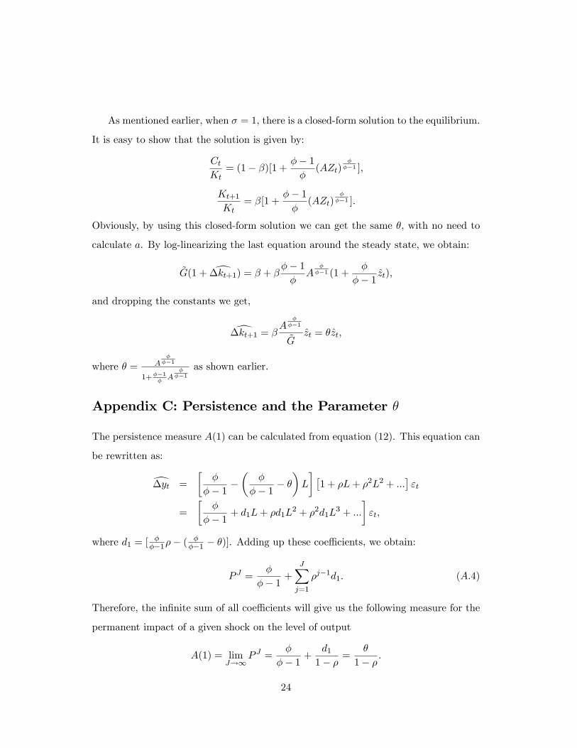
Appendix B: Parameters in the Linearization

Let xt denote the deviation of variable Xt from its steady state value in logarithms.

From the log-linearization of equation (10), we obtain the following first order stochastic

difference equation:

a1st + a2zt = a3Et (st+1) + a4Et (zt+1) , (A.1)

where

a1 =

[G

(1− S)Aφφ−1

]σσS

[A

φφ−1

G+

1

1− S

],

a2 =

[G

(1− S)Aφφ−1

]σσ

1

φ− 1

[A

φφ−1 (φS − 1)

G− φ

],

a3 = βS

1− S

{[1

(1− S)Aφφ−1

]σσ +

φ

φ− 1A

φφ−1

(1−σ) 1

1− Sσ

},

a4 = β

{A

φφ−1

(1−σ) 1

1− S(1− σ)−

[1

(1− S)Aφφ−1

]σσ

φ

φ− 1

}.

Since zt = ρzt−1 + εt, the solution is given by:

st = azt, (A.2)

where a = ρa4−a2

a1−ρa3. Note that, when σ = 1, a1 = S

1−S (φ−1φ + A

φ1−φ ), a2 = − φ

φ−1Aφ

1−φ ,

a3 = βa1, a4 = βa2, and therefore a = 1−SS

φφ−1

Aφ

1−φ

φ−1φ

+Aφ

1−φ. By plugging this value into

the expression for θ we obtain θ = Aφφ−1

1+φ−1φA

φφ−1

as reported in equation (13).

23

As mentioned earlier, when σ = 1, there is a closed-form solution to the equilibrium.

It is easy to show that the solution is given by:

CtKt

= (1− β)[1 +φ− 1

φ(AZt)

φφ−1 ],

Kt+1

Kt= β[1 +

φ− 1

φ(AZt)

φφ−1 ].

Obviously, by using this closed-form solution we can get the same θ, with no need to

calculate a. By log-linearizing the last equation around the steady state, we obtain:

G(1 + ∆kt+1) = β + βφ− 1

φA

φφ−1 (1 +

φ

φ− 1zt),

and dropping the constants we get,

∆kt+1 = βA

φφ−1

Gzt = θzt,

where θ = Aφφ−1

1+φ−1φA

φφ−1

as shown earlier.

Appendix C: Persistence and the Parameter θ

The persistence measure A(1) can be calculated from equation (12). This equation can

be rewritten as:

∆yt =

[φ

φ− 1−(

φ

φ− 1− θ)L

] [1 + ρL+ ρ2L2 + ...

]εt

=

[φ

φ− 1+ d1L+ ρd1L

2 + ρ2d1L3 + ...

]εt,

where d1 = [ φφ−1ρ− ( φ

φ−1 − θ)]. Adding up these coeffi cients, we obtain:

P J =φ

φ− 1+

J∑j=1

ρj−1d1. (A.4)

Therefore, the infinite sum of all coeffi cients will give us the following measure for the

permanent impact of a given shock on the level of output

A(1) = limJ→∞

P J =φ

φ− 1+

d1

1− ρ =θ

1− ρ.

24

Cochrane (1988) suggests another measure of persistence:

V = limJ→∞

1 + 2J∑j=1

(1− j

J + 1)ψj

, (A.5)

where ψj is the jth autocorrelation of the growth rate of output.

The persistence measure V can be calculated by rewriting equation (12) as an

ARMA(1,1) process:

(1− ρL)∆yt =

[φ

φ− 1−(

φ

φ− 1− θ)L

]εt = b1εt − b2εt−1

with b1 = φφ−1 and b2 = φ

φ−1 − θ.

The autocorrelation coeffi cients of this ARMA(1,1) process are the following: ψ1 =

ρb21−ρ2b1b2+ρb22−b1b2b21−2ρb1b2+b22)

and ψτ = ρψτ−1 for τ > 1. Given this structure for the autocorrel-

ation coeffi cients we obtain V = limJ→∞[1 + 2ψ1

∑Jj=1(1− j

J+1)ρj−1]

= 1 + 2 ψ11−ρ .

By substituting the corresponding coeffi cients b1 and b2 into ψ1:

V =

(1− ρ2

)θ2

(1− ρ)2

[(φφ−1

)2− 2ρ( φ

φ−1)(

φφ−1 − θ

)+(

φφ−1 − θ

)2] (A.6)

which is increasing in θ as long as θ < 2 φφ−1 .

Appendix D: The Moving Average Representation for

the Level of Log GNP

We can derive the MA representation (or impulse response function) for the level of log

GNP by rewriting equation (12):

yt = yt−1 + lnG+A(L)εt

= yt−1 + lnG+

[φ

φ− 1+ d1L+ ρd1L

2 + ρ2d1L3 + ...

]εt,

where d1 = [ φφ−1ρ− ( φ

φ−1 − θ)]. By iterating, we obtain:

yt = y0 + t lnG+B(L)εt

= y0 + t lnG+[B0 +B1L+B2L

2 +B3L3 + ...

]εt,

25

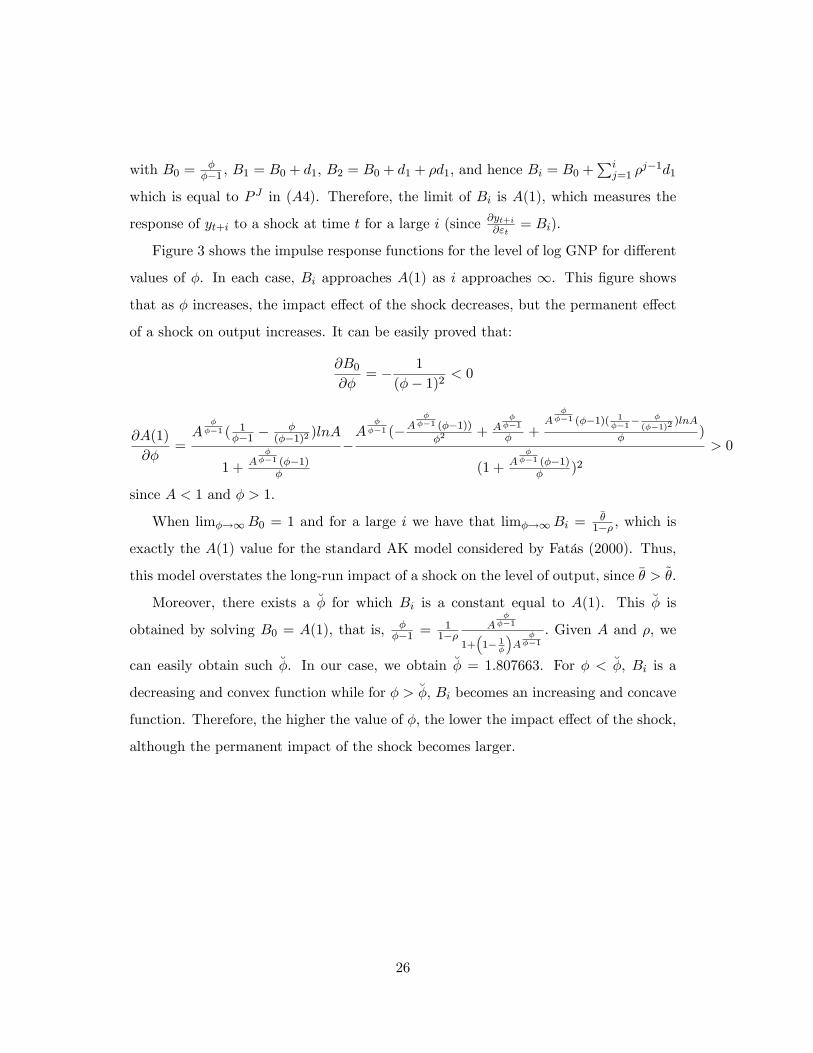
with B0 = φφ−1 , B1 = B0 + d1, B2 = B0 + d1 + ρd1, and hence Bi = B0 +

∑ij=1 ρ

j−1d1

which is equal to P J in (A4). Therefore, the limit of Bi is A(1), which measures the

response of yt+i to a shock at time t for a large i (since∂yt+i∂εt

= Bi).

Figure 3 shows the impulse response functions for the level of log GNP for different

values of φ. In each case, Bi approaches A(1) as i approaches ∞. This figure shows

that as φ increases, the impact effect of the shock decreases, but the permanent effect

of a shock on output increases. It can be easily proved that:

∂B0

∂φ= − 1

(φ− 1)2< 0

∂A(1)

∂φ=A

φφ−1 ( 1

φ−1 −φ

(φ−1)2 )lnA

1 + Aφφ−1 (φ−1)

φ

−A

φφ−1 (−A

φφ−1 (φ−1))

φ2 + Aφφ−1

φ +A

φφ−1 (φ−1)( 1

φ−1− φ

(φ−1)2)lnA

φ )

(1 + Aφφ−1 (φ−1)

φ )2

> 0

since A < 1 and φ > 1.

When limφ→∞B0 = 1 and for a large i we have that limφ→∞Bi = θ1−ρ , which is

exactly the A(1) value for the standard AK model considered by Fatás (2000). Thus,

this model overstates the long-run impact of a shock on the level of output, since θ > θ.

Moreover, there exists a φ for which Bi is a constant equal to A(1). This φ is

obtained by solving B0 = A(1), that is, φφ−1 = 1

1−ρA

φφ−1

1+(

1− 1φ

)A

φφ−1

. Given A and ρ, we

can easily obtain such φ. In our case, we obtain φ = 1.807663. For φ < φ, Bi is a

decreasing and convex function while for φ > φ, Bi becomes an increasing and concave

function. Therefore, the higher the value of φ, the lower the impact effect of the shock,

although the permanent impact of the shock becomes larger.

26

27

FIGURES

Persistence and Long-term Output Growth - 101 Countries

0

1

2

3

4

5

6

-4 -2 0 2 4 6 8 10 12 14 16

Average Per Capita Output Growth Rate, 1970-2008

Pers

iste

nce

Persistence = 4.12 + 0.05 Average Per Capita Output Growth

(66.6) (2.25)

R2=0.048

FIGURE 1: Short-term persistence and long-term output growth, 1970-2008

Long-term Output Growth and Depreciation -101 Countries

-4

-2

0

2

4

6

8

10

12

14

16

0 5 10 15 20 25

Average Depreciation Rate, 1970-2008

Ave

rag

e P

er

Ca

pit

a O

utp

ut

Gro

wth

Rate

Average Per Capita Output Growth = - 0.04 + 0.16 Depreciation Rate

(-0.06) (3.23)

R2=0.10

FIGURE 2: Depreciation and long-term output growth, 1970-2008

28

29

TABLES

TABLE 1: LSDV Panel Growth Estimations

(1)

LSDV

(2)

LSDV

(3)

LSDV

(4)

LSDV

OECD Full Sample

Depreciation a 0.039*** 0.057*** 0.045*** 0.042***

(4.87) (3.65) (6.43) (5.33)

NFCF a 0.004** 0.008*** 0.011*** 0.009***

(2.20) (2.94) (6.10) (3.92)

Population Growth -0.009** -0.009***

(-2.40) (-3.58)

Trade a 0.011 0.028***

(0.61) (3.02)

Secondary Schooling a -0.008 -0.009

(-0.83) (-1.13)

Agriculture Share a 0.002 -0.002

(0.49) (-0.75)

Lag GDP p.c. a -0.036*** -0.028***

(-2.92) (-3.59)

Specification Tests

Wald (joint)

26.20

[0.000]

86.10

[0.000]

47.61

[0.000]

116.7

[0.000]

Wald (Dummy)

792.5

[0.000]

9885

[0.000]

755.6

[0.000]

381.2

[0.000]

Wald (time)

734.6

[0.000]

1086

[0.000]

489.6

[0.000]

1.290e+004

[0.000]

AR(1) test

3.688

[0.000]

0.079

[0.937]

3.087

[0.002]

1.355

[0.175]

AR(2) test

2.030

[0.042]

-0.453

[0.650]

-0.408

[0.683]

-1.226

[0.220]

R2 0.355 0.439 0.264 0.363

Observations 981 393 3347 1124

Notes: The dependent variable is the growth rate of real per capita output. a indicates

that the variable is included in the regression in log-levels. *,** and *** indicate

significance at 10%, 5% and 1%, respectively. Robust t-statistics are given in

parenthesis. Figures in brackets for the specification tests represent probabilities of non-

rejection of the null hypothesis. A Wald-type test is given under the name Wald

(dummy) to test for the joint-significance of the deterministic components given by the

constant and time effects. Wald(joint) tests for the joint-significance of both the long-

run and the short-run coefficients. All Wald-type tests are distributed as a χ2 with the

number of degrees of freedom equal to the number of restrictions. The tests labelled by

AR(1) and AR(2) test for the presence of first and second-order correlation in the

residuals of the model.

30

Table 2: Dynamic Panel Growth Estimations

(5)

SYS-GMM

(6)

SYS-GMM

(7)

SYS-GMM

(8)

SYS-GMM

OECD Full Sample

Depreciation a 0.033*** 0.061*** 0.048*** 0.041*** (4.62) (4.20) (4.27) (4.96)

NFCF a 0.003** 0.009*** 0.011*** 0.008***

(2.05) (3.15) (3.82) (3.03)

Population Growth -0.009* -0.007 **

(-1.89) (-2.29)

Trade a 0.004 0.037***

(0.21) (3.11)

Secondary Schooling a -0.004 -0.015*

(-0.32) (-1.88)

Agriculture Share a 0.003 -0.001

(0.78) (-0.41)

Lag GDP p.c. a -0.059*** -0.035***

(-2.71) (-2.62)

Specification Tests

Wald (joint)

22.38

[0.000]

102.8

[0.000]

18.72

[0.000]

62.09

[0.000]

Wald (dummy)

867.2

[0.000]

3.494e+004

[0.000]

858.5

[0.000]

395.2

[0.000]

Wald (time)

757.3

[0.000]

1001.

[0.000]

405.9

[0.000]

3787

[0.000]

AR(2) test

-2.628

[0.009]

0.2732

[0.785]

-2.413

[0.016]

-0.500

[0.617]

Sargan test

1599

[0.014]

794.2

[1.000]

3241

[0.000]

1810

[1.000]

Observations 981 393 3347 1123

Notes: The dependent variable is the growth rate of real per capita output. a indicates that the variable is

included in the regression in log-levels. *,** and *** indicate significance at 10%, 5% and 1% ,

respectively. Robust t-statistics are given in parenthesis. Figures in brackets for the specification tests

represent probabilities of non-rejection of the null hypothesis. A Wald-type test is given under the name

Wald (dummy) to test for the joint-significance of the deterministic components given by the constant and

time effects. Wald(joint) tests for the joint-significance of both the long-run and the short-run coefficients.

All Wald-type tests are distributed as a χ2 with the number of degrees of freedom equal to the number of

restrictions. All the models are estimated with the system estimator of Arellano and Bover (1995). The

Sargan statistic for over-identifying restrictions testing the validity of the instruments under the null

hypothesis is distributed as a χ2 with J-K degrees of freedom, where J is the number of instruments and K

is the number of regressors. The AR(2) statistic tests for the presence of second-order correlation in the

residuals of the model and is distributed as a standard normal distribution.

31

TABLE A1: Descriptive Statistics

Country Name

Code

Per Capita

Output Growth

Depreciation Rate

Net Investment

Rate

Mean Std Error Mean Std Error Mean Std Error

1 Austria AUT 2.42 1.75 17.45 3.10 6.60 3.17

2 Belgium BEL 2.20 1.81 16.34 2.72 4.29 3.30

3 Denmark DNK 1.80 1.88 17.16 2.73 3.41 3.27

4 Finland FIN 2.67 2.86 18.68 3.27 4.61 4.88

5 France FRA 1.98 1.61 14.08 2.44 6.75 3.13

6 Germany DEU 2.04 1.57 16.06 2.69 5.54 3.47

7 Greece GRC 2.38 3.29 12.81 2.26 9.18 4.00

8 Hungary HUN 2.69 3.41 13.86 3.65 10.98 6.71

9 Iceland ISL 2.84 3.38 16.51 3.79 7.33 4.13

10 Ireland IRL 3.87 3.06 11.68 2.18 9.97 3.79

11 Italy ITA 2.04 2.05 17.22 2.89 4.96 3.14

12 Luxembourg LUX 3.07 3.24 18.30 4.88 2.64 4.82

13 Netherlands NLD 2.09 1.55 16.60 2.68 5.24 3.40

14 Norway NOR 2.77 1.64 19.00 2.98 5.50 4.29

15 Portugal PRT 2.86 3.80 19.07 3.86 6.42 4.82

16 Spain ESP 2.35 2.00 16.54 3.19 7.86 3.26

17 Sweden SWE 1.88 1.93 13.50 2.24 5.76 2.97

18 Switzerland CHE 1.15 2.12 20.23 3.90 4.95 3.87

19 Turkey TUR 2.41 3.91 8.07 3.82 11.19 4.67

20 United Kingdom GBR 2.13 1.89 14.85 2.86 3.29 2.72

21 Australia AUS 1.87 1.65 20.00 4.07 5.82 3.35

22 China CHN 7.86 3.88 12.16 3.42 19.71 5.33

23 Hong Kong HKG 4.83 4.43 15.73 2.42 9.34 4.15

24 Indonesia IDN 4.21 3.60 8.01 3.29 16.92 4.97

25 Japan JPN 2.46 2.49 19.75 3.35 9.39 5.29

26 Korea Rep KOR 5.61 3.42 13.96 2.72 16.35 4.20

27 Malaysia MYS 4.08 3.59 12.91 2.46 15.34 6.94

28 New Zealand NZL 1.16 2.39 16.70 3.06 5.95 3.49

29 Philippines PHL 1.41 3.32 10.41 2.22 10.35 5.75

30 Singapore SGP 5.16 3.96 16.01 3.40 18.53 7.76

31 Thailand THA 4.56 3.85 11.67 2.42 16.84 6.03

32 Argentina ARG 1.25 5.95 13.48 4.78 8.43 6.12

33 Bolivia BOL 0.57 3.04 9.87 1.56 5.93 2.86

34 Brazil BRA 2.31 3.99 13.05 3.26 6.43 3.73

35 Chile CHL 2.83 5.00 16.98 4.57 3.02 5.99

36 Colombia COL 2.07 2.30 11.81 2.40 5.94 2.14

37 Costa Rica CRI 2.21 3.39 11.38 6.67 8.99 5.28

38 Dominican Rep. DOM 3.43 4.19 8.33 3.40 11.34 4.93

39 Ecuador ECU 1.81 3.59 13.60 3.43 6.36 4.02

40 El Salvador SLV 1.03 4.15 8.58 3.52 7.29 4.07

41 Guatemala GTM 1.17 2.40 11.05 1.50 4.47 2.45

42 Honduras HND 1.31 3.06 7.29 1.79 14.83 4.54

43 Jamaica JAM 0.68 4.77 10.17 2.51 12.27 5.18

44 Mexico MEX 1.71 3.30 12.23 2.38 7.70 2.26

45 Nicaragua NIC -0.75 6.36 10.04 2.79 11.35 6.10

46 Panama PAN 2.03 4.48 8.61 1.53 9.58 4.46

32

47 Paraguay PRY 1.86 3.91 11.33 3.69 9.75 2.95

48 Peru PER 1.11 5.47 9.87 3.37 10.89 4.92

49 Uruguay URY 1.91 5.13 10.57 4.93 4.47 6.53

50 Venezuela VEN 0.13 5.65 13.42 3.30 8.99 5.61

51 Algeria DZA 1.35 5.16 10.50 3.17 19.65 6.23

52 Egypt EGY 3.09 2.83 9.04 2.21 12.40 5.40

53 Iran Islamic Rep. IRN 1.46 7.24 22.45 13.31 5.40 16.08

54 Israel ISR 2.25 2.73 17.96 2.98 4.51 4.73

55 Jordan JOR 2.65 6.76 9.50 3.08 17.12 7.94

56 Morocco MAR 2.16 4.25 10.82 1.94 12.42 4.98

57 Saudi Arabia SAU 1.23 7.94 16.01 10.56 3.54 12.94

58

Syrian Arab

Republic SYR 2.21 7.16 11.20 2.50 11.66 5.74

59 Tunisia TUN 3.25 3.42 11.08 1.83 14.42 4.24

60 Canada CAN 1.87 2.01 14.31 1.26 6.76 1.80

61 United States USA 1.90 2.00 12.86 1.01 5.93 1.11

62 Bangladesh BGD 1.52 4.03 9.55 2.78 10.40 3.76

63 India IND 3.27 3.17 10.73 1.84 10.84 3.96

64 Nepal NPL 1.48 2.64 5.04 2.46 13.83 3.80

65 Pakistan PAK 2.37 2.40 10.84 2.02 5.71 2.58

66 Sri Lanka LKA 3.32 2.07 5.94 1.65 16.54 4.72

67 Benin BEN 0.50 3.02 8.54 2.26 7.46 4.01

68 Botswana BWA 6.67 5.41 15.23 3.91 12.77 7.49

69 Burkina Faso BFA 1.60 3.16 8.17 2.20 10.36 3.72

70 Burundi BDI 0.27 5.41 5.58 1.68 5.44 5.60

71 Cameroon CMR 1.09 5.92 10.07 3.39 10.33 7.39

72

Central African

Republic CAF -0.99 4.02 8.36 1.93 1.52 3.09

73 Chad TCD 0.94 9.27 8.29 3.01 5.53 12.94

74 Congo Dem Rep ZAR -3.05 5.23 7.67 2.08 3.64 5.26

75 Congo Rep. COG 1.63 6.00 15.32 5.53 11.94 9.70

76 Cote d'Ivoire CIV -1.08 4.23 8.89 2.95 6.29 7.38

77 Equatorial Guinea GNQ 13.54 19.16 15.01 8.31 32.11 28.46

78 Gabon GAB 1.37 10.89 15.94 8.12 15.65 9.12

79 Gambia The GMB 0.63 3.27 11.36 3.55 8.54 4.04

80 Ghana GHA 0.59 4.49 8.76 1.72 7.15 8.43

81 Guinea-Bissau GNB -0.18 7.57 7.39 1.51 17.90 9.25

82 Kenya KEN 1.01 4.34 9.29 2.00 9.52 3.10

83 Lesotho LSO 2.94 6.58 8.41 2.95 29.20 16.32

84 Liberia LBR -2.27 20.49 8.60 3.00 2.46 6.04

85 Madagascar MDG -1.00 4.39 8.42 3.06 5.03 6.50

86 Malawi MWI 0.77 5.53 7.94 2.18 9.94 5.41

87 Mali MLI 1.63 5.18 7.45 2.77 11.82 4.77

88 Mauritania MRT 0.13 4.37 9.32 1.77 11.92 15.83

89 Mauritius MUS 3.51 3.47 12.53 2.50 11.42 3.45

90 Niger NER -1.17 6.04 6.96 2.33 5.42 5.17

91 Nigeria NGA 1.58 6.31 7.71 4.72

92 Rwanda RWA 1.73 10.95 6.98 2.43 7.97 3.05

93 Senegal SEN 0.16 3.67 10.11 3.28 8.68 4.57

94 Sierra Leone SLE 0.26 7.09 8.85 3.01 1.85 4.13

95 South Africa ZAF 0.60 2.45 15.84 3.43 5.07 5.18

96 Sudan SDN 2.10 5.79 9.73 3.03 3.04 4.02

97 Swaziland SWZ 2.72 4.07 11.24 3.03 9.82 8.92

98 Togo TGO -0.38 5.74 8.21 2.13 9.42 3.67

33

99 Uganda UGA 2.54 3.22 8.37 2.78 5.62 5.89

100 Zambia ZMB -0.90 4.03 12.04 4.45 6.45 7.96

101 Zimbabwe ZWE -0.22 6.25 10.08 4.69 7.04 6.84

Notes: The real per capita GDP growth figures that appear in the Table are multiplied

by 100. Net Investment Rate stands for real Net Fixed Capital Formation over real

GDP. The depreciation of fixed capital measured as a proportion of GDP represents

the consumption of fixed capital as given by the replacement value of capital used up

in the production process. The source of these data is the World Development

Indicators of the World Bank (2009).