Endogenous Groups and Dynamic Selection in

Mechanism Design∗

Gabriel A. Madeira Robert M. Townsend

January 23, 2007

Abstract

We create a dynamic theory of endogenous risk sharing groups, with good internal in-

formation, and their coexistence with relative perfomance, individualistic regimes, which

are informationaly more opaque. Inequality and organizational form are determined si-

multaneously. Numerical techniques and succinct re-formulations of mechanism design

problems with suitable choice of promised utilities allow the computation of a stochastic

steady state and its transitions. Regions of low inequality and moderate to high wealth

(utility promises) produce the relative performance regime, while regions of high inequality

and low wealth produce the risk sharing group regime. If there is a cost to prevent coali-

tions, risk sharing groups emerge at high wealth levels also. Transition from the relative

performance regime to the group regime tend to occur when rewards to observed outputs

exacerbate inequality, while transitions from the group regime to the relative performance

regime tend to come with a decrease in utility promises. Some regions of inequality and

wealth deliver long term persistence of organization form and inequality, while other re-

∗We are thankful to the associate editor and the referee, and to participants of the MIT macro lunch, the

University of Chicago Theory Seminar, Workshop on Applied Dynamic Economics and General Equilibrium,

and the Economic Theory and Development Working Group for helpful comments.

1

gions deliver high levels of volatility. JEL Classification Numbers: D23,D71,D85,O17.

Keywords: Risk sharing, incentives, mechanism design, relative performance, networks.

1 Introduction

Imagine a landowner with two distinct plots of land and two possible tenants. One possible

arrangement is for the two tenants to form a cropping group and farm all the land of the owner

as a cooperative association, deciding on inputs and sharing outputs after paying the land

rental. Another possible arrangement is for the landowner to rent to each of the two tenants

individually, using a comparison across the plot harvests to determine the net rental payment,

awarding an apparently diligent agent with a larger ex post share of the harvest. Both of

these are a stylized version of what we see in tenancy data in villages in Maharastra, India,

as described in more detail in Townsend and Mueller [29] and Mueller, Prescott and Sumner

[19]. Some principals have their land farmed by single cropping groups while others divide up

the land, farmed by several individual tenants. This gives us the first empirical observation:

there is cross sectional diversity in organization arrangements, with some individuals acting

cooperatively as in risk sharing groups, and others competitively, as in a relative performance

arrangement.

A second empirical observation is that organization form changes over time. At the end

of the season, some groups disband (or at least their composition changes). Likewise, tenants

previously acting as individuals now agree to form a group (or at least enter into an existing

group). Though the sample size and number of time periods were too limited to know for

sure, the retrospective data in the Townsend and Mueller study are not inconsistent with the

possibility that a given land owner might switch from one type of regime to another even with

the same set of tenants, the latter as a risk sharing group in one period and competing under

relative performance in another. Certainly flux in groups is typical of the longer village history.

More generally, sociologists with an interest in social networks have typically found them to

2

be unstable. There is low correlation in the composition of networks over time and occasional

abandonment: to cite just one example Barkey and van Rossem [3] analyzes 17th-century

Ottoman villages in western Anatolia, using court records to reconstruct formal and informal

networks. Under conditions of state and market expansion, those villages in intermediate

positions in the regional structure tend to experience the vagaries of these changes more than

central or isolated villages. Ironically, cooperative village organization in these intermediate

villages is found to promote contention. Sociological theorists Leik and Chalkey [17] discuss

a list of possible causes of instability documented in this and many other studies: unreliable

measurement, external change, inherent instability, and systematic change from endogenous

forces.

Development economists with an interest in networks seem, on the other hand, to fix apriori

the likely network candidate and then test for risk sharing. Often the village is taken as the

obvious group, as in Townsend [28] study villages in india. But several of the cropping groups

mentioned above at the outset of this introduction exist in Aureapple, one of these villages. This

raises the question of whether the correct candidate for a risk sharing network is a village or one

of these groups . Others study the nuclear family in Ethiopia (Dercon and Krishnan [7]), tribes

in Cote D’Ivoire as in Grimard [11], and family and friends in the Phillipines (Fafchamps and

Lund [9]). Some find networks and subgroups that share risk well, but other reject the selected

apriori candidate. Chiappori, et al [6] shows in particular that some family-related networks

within Thai villages, and some villages, pass rigorous tests for risk sharing while other networks

and village perform poorly. It seems the search for a stable apriori structure may be misguided.

Rather, economists and sociologists need theories to deal empirically with cross sectional

variety and temporal change. Of course different disciplines, and different theories within a

discipline, are likely to suggest different candidate variables as crucial. In this regard we are

muchmotivated by one salient piece of evidence for a theory of joint liability credit groups. Ahlin

and Townsend [1] test the group-versus-relative performance model of Prescott and Townsend

[24], Itoh [13] and Holmstrom and Milgrom [12], finding that the higher the level of inequality in

3

a village, and the lower the overall wealth of the village, the more likely it is that two (or more)

households will borrow in a group. Conversely, relative equality is a force for individual loans.

Consistent with this, but not tested, is the notion that inequality and organization structure

are co-determined and that both can change over time. After all, the relative performance

regime has the natural implication that some agents would be punished and other rewarded,

so that starting from equality and relative performance, there would be switches to inequality

and groups. In the other direction, starting from inequality and groups, successful outcomes

can increase wealth and cause a switch to a more individualistic regime.

What we did not anticipate, from the data or our initial thinking, is that depending on the

staring point, one could see long periods with a stable regime, either risk sharing networks or

individualist structures, then periods of volatility with a switch back and forth across organi-

zation structure many times in relatively few periods. We show how in principle this model

would be tested, with cross section data and a sufficiently long panel.

Various other authors have taken up the challenge of producing a theory of groups or

networks, that is, making groups or group size endogenous. Kranton and Bramoullé [16] model

networks as the costly formation of bilateral links. Their setup allows heterogenous treatment

of otherwise identical individuals. In a dynamic version with exogenous pairwise meetings

probabilities, the size of a dynamic network grows and shrinks over time with agents at the fringe

at risk of being cut-off entirely. Related is Jackson and Watts [14] who focus on self-improving

and myopic paths. In contrast, Genicot and Ray [10] consider a static model with a core notion

of outcomes, that is, the possibility that subgroups of individuals may destabilize insurance

arrangements among the larger group. Self-enforcing risk-sharing agreements are robust not

only to single-person deviations but also to potential deviations by subgroups. However, such

deviations must be credible, in the sense that the subgroup must pass exactly the same test

that is applied to the entire group. Stable groups have bounded size and the degree of risk

sharing is non-monotonic in risk.

Also delivering clusters but with varying internal risk sharing is the paper of Murgai, Win-

4

ters, Sadoulet and deJanvry [20]. High association costs combined with low extraction costs

lead to clusters with full insurance, while low association costs with high extraction costs will

lead to community-level partial insurance. Empirical results from data on water exchanges

among households along irrigation canals in Pakistan are used to support this proposition.

Here, in our paper, we take a dynamic, foresighted, mechanism design approach with infor-

mation as an explicit impediment to trade. This connects us to a mechanism design literature

with its focus on information and theories of inside and outside monies. Cavalcanti and Wallace

[5] study implementable allocations in a random matching model in which some people have

publicly known histories (banker) and others have private histories (non-bankers). Bankers

can issue bank notes, to be compared with outside money. Though outside money dominates,

Mills [18] shows that information lags for bankers can deliver the combined use of both kinds

of monies. For us, groups have good internal information though the outsider does not, while

individuals in relative performance have limited information as with the principal. Our re-

sults show that diverse information structures and organization forms can coexist and evolve

in interchangeable forms.

We characterize the solution to the multiagent moral hazard model problem as a linear

program. At this point, a curse of dimensionality emerges - a common problem in the linear

programing solutions of contract problems, exacerbated here by the presence of more than one

agent. We develop a formulation that makes computational implementation less demanding.

The basic idea of this reformulation is to solve the moral hazard problem using a variable that

summarizes utilities from consumption and promises to the future, instead of using consumption

and promises directly. This formulation can be useful for multiagent dynamic moral hazard

problems in general and facilitates empirical work.

The paper is organized as follows. In section 2 we present the model, that is basically a

dynamic extension of the formulation of Prescott and Townsend [23]. In section 3 we prove

some propositions about the dynamics of the model. In particular, we show that incentives for

effort make the dynamics depend on output. The presence of outside options for agents and the

5

principal can make the feasible set compact and rule out degenerate steady states. Section 4

presents and discusses numerical results obtained. The numerical procedure adopted, including

some computationally convenient reformulations of the problem, is discussed in details in the

appendix.

2 The Model

2.1 Environment:

A local economy has three individuals, two agents with preferences as discounted expected

utilities over consumption and effort, and a principal, whose objective function is the present

value of the surplus of production over the agents’ consumption. The utility of agent i at period

t is wti ≡ E{PT

s=t βs−t[U(csi ) + V (esi )]}, where cti and eti are, respectively, the consumption and

the effort of agent i at period t, and β is a subjective discount factor. Function U is strictly

concave and strictly increasing. The function V (e) is strictly decreasing, meaning that agents

prefer to make low effort. The production technology is characterized by p(qt1, qt2 | et1, et2) > 0,

a probability distribution of outputs at t that depends on the effort levels of both individuals

within the period. This allows correlated outputs. The present value of the principal’s surplus

flow at t is given by St ≡PTs=t

¡11+r

¢s[qs1 + qs2 − cs1 − cs2], where r is an exogenous interest rate,

as if this were a small open economy. We assume that 11+r

= β. For expositional convenience we

denote the vectors (ct1, ct2), (q

t1, q

t2) and (e

t1, e

t2) by c

t, qt and et, respectively. The sets of possible

consumption, effort and output for each individual in each period are denoted, respectively, by

C, Q and E. Thus consumption, effort and output pairs are, respectively, in C2, Q2 and E2.

We study allocations that are efficient conditional on the following moral hazard problem:

the principal does not observe the efforts of the agents, although it is possible to allow one agent

to observe the effort of the other. This implies that the decision of how much effort is done is

ultimately taken by the agents. The decision process depends on how the agents are organized.

Two regimes are available: a group regime in which individuals are allowed to communicate

6

and thus to collude and jointly define levels of effort and share risks, and a relative performance

regime in which individuals are not allowed to communicate and collude. Inside a group, each

agent can enforce actions defined in an agreement (or contingent plan). But the members of

a group can collude against the principal and take actions and consumption levels that are

not recommended in the initial plan, if this can benefit the agents of the group. Therefore,

the choices inside a group maximize a sum of utilities weighted by underlying internal Pareto

weights. While in the relative performance regime each individual decides how much effort to

do, in the group regime this decision is taken jointly, according to the Pareto weights inside the

group. We assume that the implementation of the relative performance regime has a fixed cost

of k that represents the cost of avoiding collusion, communication and side payments among

individuals.

The type of collective organization at a given date is characterized by the regime (relative

performance or groups), and in the case of groups, by the inside-group utility weights. We define

O as the set of types of organization available. The elements of O characterize the regime, and

for the groups regime, the Pareto weight inside groups. We denote the set of possible utility

weights inside groups by M.

2.2 The Mechanism Design Program

Our goal is to find allocations that are efficient given the environment and the organizational

forms available. We formulate the overall Pareto problem as a maximization of the expected

surplus of an outsider contractor, that we call the principal, conditional on initial promised

utility levels for the two agents. This formulation may make it appear that the principal is

the one making decisions about the choice of regime, but this is just a way to allow us to find

the set of information-constrained Pareto optimal allocations, varying with the initial promise

vector. The Mechanism Design problem thus determines the optimal state contingent historical

path of the type of organization to which agents are assigned, their vectors of consumption,

effort and output, and the surplus of the principal. The constraints on the problem include a

7

set of incentive and technological constraints.

We follow Phelan and Townsend [21] and solve the problem sequentially. At each period the

distribution of consumption, effort, organization and future expected utilities are defined by

a principal-multiagent problem conditional on initial promises. This recursive formulation of

the problem is not restrictive, since expected utilities from the future and their corresponding

surplus levels are sufficient to characterize all incentives that come from future arrangements.

Finally, for simplicity1 and realism, we require that arrangements be renegotiation proof i.e.,

they do not allow gains for all individuals resulting from renegotiation between the principal

and the agents, as could be the case if the surplus function were non decreasing in one or both

utility promises.

More formally, at any period, t, a principal multi-agent problem defines a probability dis-

tribution over the elements of Γt ≡ C2 × Q2 × E2 × O ×W 2, which are vectors expressing

consumption, output and effort vectors, the type of organization that individuals are part of

and the pair of expected future utilities. The distribution of consumption, output, effort and

the type of organization in future periods is implied by the choices of promised future utilities

wt+11 and wt+1

2 . Throughout the remainder of the paper, we call (wt1, w

t2) the ex-ante utility

pair at t, and (wt+11 , wt+1

2 ) the set of promised (future) utilities assigned at t. For notational

convenience, we sometimes omit the index t on variables and refer to the initial pair of expected

utilities as w and the pair of promised utilities as w0. Again, the surplus of the principal at t is

St(w) and at t+1, St+1(w0) where the superscript t can also be deleted as in an infinite period

problem.

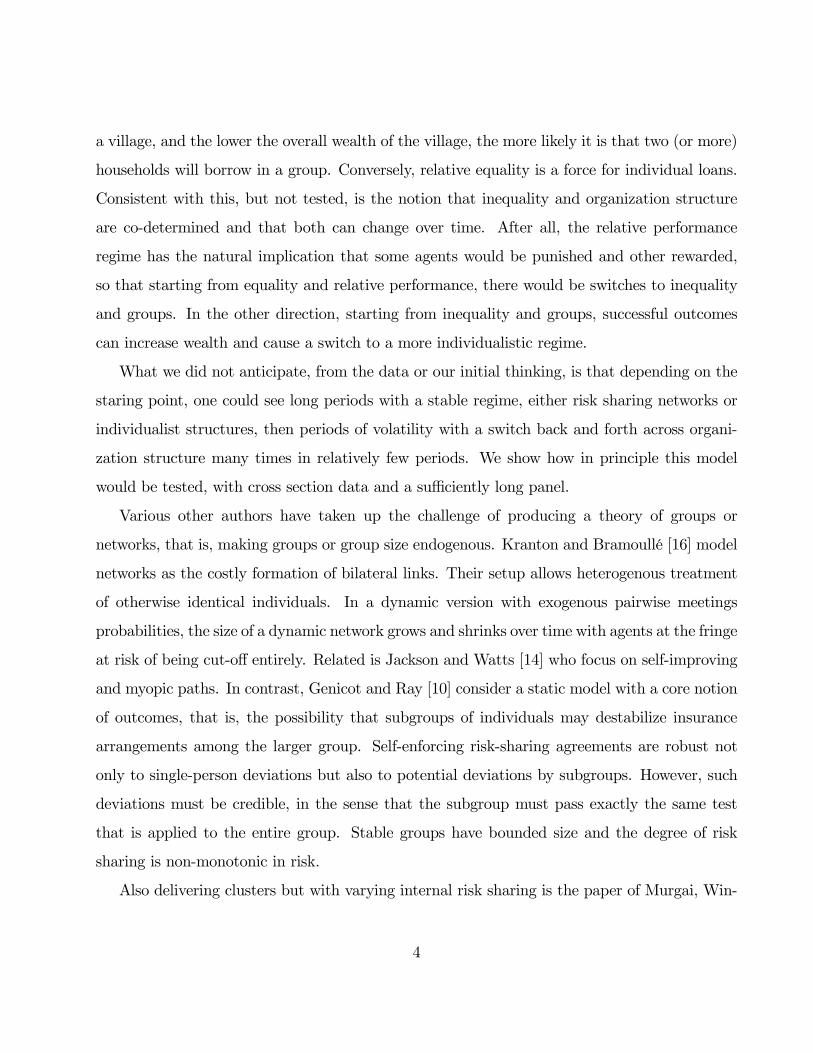
The sequence of events in period t is presented in Figure 1. First, agents are assigned to

a regime: groups or the relative performance. When they are assigned to the group regime,

utility weights inside the groups are defined. Then, the agents or the group decide their amount

of effort (et1, et2). Following the employment of effort, an output pair (q

t1, q

t2) is obtained and

1Although the non-renegotiation requirement imposes additional constraints to the problem, it is helpful in

obtaining numerical solutions since it guarantees that the surplus maximization problem is equivalent to utility

maximization conditional on the surplus level.

8

observed by the principal. Finally, conditional on the output, a consumption pair (ct1, ct2) and

a pair of promised expected utilities (wt+11 , wt+1

2 ) is assigned.

Figure 1

Whenever individuals join an organization o, an ex-ante organization-specific utility pair,

denoted wo ∈W 2 is implied. The arrangement given o and wo must be renegotiation proof, in

the sense that there is no possibility of utility improvement to the agents or the group without

a lower surplus to the principal. We can assume, without loss of generality, given the choice

of organization o and a corresponding organization specific utility pair wo, the level of effort e,

and the output of each agent, that the choices of consumption and promises for each agent are

deterministic 2. Therefore, given the vector of initial promises w, the vectors of consumption

c and promises for the future w0 can be written as functions of output q, effort e, organization

o,and a utility pair generated under this organization wo. Here again, o ∈ O represents the

2Notice that consumption is separable from efforts in utility. From the fact that the utility function is concave

and promises can be redefined as the expected values of some initial randomization, given any arrangement that

has randomization of c and w0, identical utility with no smaller surplus can be obtained without randomization

of c and w0, without affecting incentive constraints. If the initial arrangement is renegotiation proof, the second

one is also renegotiation-proof. In any event, we can generate randoness in w0 by varying w0o. For a more explicit

formulation which allows general randomization in promises and consumption see the Appendix.

9

organizational form, and we use the notation o = µ when the regime is groups with internal

utility weights µ ∈ M , and o = r, when the regime is relative performance. Randomization

between different arrangements under the same regime is allowed3, so the decision variable

includes not only a lottery over the choice of organization, but also randomization of utility

pairs wo for each organization o. We assume that Q, E and O are finite sets. For efforts and

outputs, a finite grid has a natural interpretation: E has two elements eh and el, denoting high

and low effort, respectively, and Q has two elements qh and ql, denoting success and failure,

respectively. Since the Pareto weights for each individual inside a group, in principle, could

have any value between zero and one, the set of possible organizations is more naturally a

continuum, that is approximated here with a fine grid.

We may also assume that whenever agents are assigned to some type of organization, they

must have an expected utility that is not smaller than some exogenously given value, that

corresponds to an outside option. For example, they could be entirely on their own, with the

utility from production in autarky, or possibly a lower value, if there is some punishment or

social stigma from abandoning the link with the principal and the other agent. Similarly, we

may assume that the principal can walk away to some outside option, so arrangements are

subject to a lower bound in the level of surplus to the principal or equivalently, an upper bound

in the set of promises to the agent. These bounds are not always imposed, and we point out

where they are utilized in the exposition below.

The set of choice variables of the principal-agent problem consists of four objects. First, the

probabilities of each organizational form and corresponding utility pair generated under this

organizaional form, Pr(o, wo | w). Second, the probabilities of effort levels for each choice oforganization and organization-specific utilities, Pr(e | o, wo, w). Finally, functions c(q, e, o, wo |w) and w0(q, e, o, wo | w), that determine the values of consumption and promises conditional

3Randomization given the same organization may be useful because given Pareto weights µ, it is possible that

w∗µ and w∗∗µ are feasible and renegotiation proof given µ, but some utility level wl

µ that is a convex combination

of w∗µ and w∗∗µ is not renegotiation proof given µ. Randomization across the two points, each of which is

renegotiation proof can generate the utility pair wlµ.

10

on outputs, effort levels, organizational form, and utility under organization.

The probability functions Pr(o, wo | w) and Pr(e | o, wo, w) are summarized by the joint

probability distribution:

Pr(q, e, o, wo | w) ≡ p(q | e) · Pr(e | o, wo, w) · Pr(o, wo | w), (1)

where p(q | e) is determined by the technology. Indeed, for expositional convenience, we

characterize the problem in terms of the joint distribution Pr(q, e, o, wo | w), but for this to beconsistent with the technology, the choice object Pr(e, q, o, wo | w) must be constrained by:

Pr(bq, be, bo, bwo | w) = p(bq | be)Xq

Pr(q, be, bo, bwo | w) (2)

∀(bq, be, bo, bwo) ∈ Q2×E2×O×W 2 ≡ X. The choice variable is thus{Pr(q, e, o, wo | w), c(q, e, o, wo |w), w0(q, e, o, wo | w) : q ∈ Q2, e ∈ E2, o ∈ O,wo ∈ W 2} ∈ Y , where Y is the set of functions

from X to [0, 1]× C2 ×W 2.

Any choice y(w) ∈ Y determines a distribution of effort, output, consumption and promises

conditional on each type of organization and corresponding organization-specific utlities. We

denote these distribution of variables conditional on organization o with sutplus wo by y(o, wo |w) = {Pr(q, e | o, wo, w), c(q, e, o, wo | w), w0(q, e, o, wo | w)}, where Pr(q, e | o, wo, w) ≡Pr(q, e, o, wo, | w)/

Pe,q

Pr(q, e, o, wo, | w). This is a function from Q2 × E2 to [0, 1] × C2 ×W 2

which is completely characterized by the function y(w) with the domain restricted to o = o and

wo = wo. Notice that :

Xq,e

Pr(q, e | o, wo, w) = 1 (3)

Further and critical, some of the constraints of the problem are specific of the organization

adopted and the corresponding organization specific utility level.

Group Constraints Inside a group, agents can enforce any agreement (or contingent plan),

but they can also collude and take decisions that are not recommended in the initial plan if

11

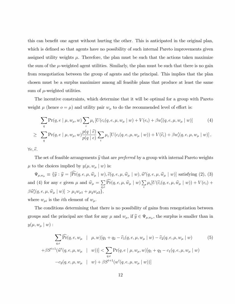
this can benefit one agent without hurting the other. This is anticipated in the original plan,

which is defined so that agents have no possibility of such internal Pareto improvements given

assigned utility weights µ. Therefore, the plan must be such that the actions taken maximize

the sum of the µ-weighted agent utilities. Similarly, the plan must be such that there is no gain

from renegotiation between the group of agents and the principal. This implies that the plan

chosen must be a surplus maximizer among all feasible plans that produce at least the same

sum of µ-weighted utilities.

The incentive constraints, which determine that it will be optimal for a group with Pareto

weight µ (hence o = µ) and utility pair wµ to do the recommended level of effort is:Xq

Pr(q, e | µ,wµ, w)Xi

µi [U(ci(q, e, µ, wµ | w) + V (ei) + βw0i(q, e, µ, wµ | w)] (4)

≥Xq

Pr(q, e | µ,wµ, w)p(q | be)p(q | e)

Xi

µi [U(ci(q, e, µ, wµ | w)) + V (bei) + βw0i(q, e, µ, wµ | w)] ,

∀e, be.The set of feasible arrangements by that are preferred by a group with internal Pareto weights

µ to the choices implied by y(µ,wµ | w) is:Ψµ,wµ ≡ {by : by = [cPr(q, e, µ, bwµ | w),bc(q, e, µ, bwµ | w), bw0(q, e, µ, bwµ | w)] satisfying (2), (3)

and (4) for any e given µ and bwµ =Pq,e

cPr(q, e, µ, bwµ | w)Pi

µi[U(bci(q, e, µ, bwµ | w)) + V (ei) +

β bw0i(q, e, µ, bwµ | w)] > µ1wµ1 + µ2wµ2},where wµi is the ith element of wµ.

The conditions determining that there is no possibility of gains from renegotiation between

groups and the principal are that for any µ and wµ, if by ∈ Ψµ,wµ , the surplus is smaller than in

y(µ,wµ | w) :Xq,e

cPr(q, e, wµ | µ,w)[q1 + q2 − bc1(q, e, µ, wµ | w)− bc2(q, e, µ, wµ | w) (5)

+βSt+1( bw0(q, e, µ, wµ | w))] <Xq,e

Pr(q, e | µ,wµ, w)[q1 + q2 − c1(q, e, µ, wµ | w)

−c2(q, e, µ, wµ | w) + βSt+1(w0(q, e, µ, wµ | w))]

12

Thus an increase in the µ-weighted sum of utilities would require some loss to the princi-

pal. Notice that this implies that the surplus function is strictly decreasing: higher utility for

the group must produce lower surplus. Condition (5) determines that whenever some internal

Pareto weight µ is assigned to a group, the choices conditional on this organizational form

maximize the µ weighted sum of utilities conditional on the surplus they produce. But notice

that (5) also implies that inside a group there is full risk sharing4. The consumption of indi-

viduals depend only on the aggregate consumption and on the Pareto weights inside the group.

Specifically, agent levels of consumption at any period t must satisfy cti = ci(µ, ca), where the

function ci(µ, ca) is defined by the following subproblem generating the groups risk sharing rule:

(c1(µ, ca), c2(µ, ca)) = arg max(c1,c2)∈C2

µ1U(c1) + µ2U(c2),

s.t.

c1 + c2 = ca,

where, again, ca is the aggregate consumption (with values on C + C = 2C). This property

gives us the interpretation of a group as a risk sharing network.

Relative Performance Constraints In the relative performance regime, agents are pre-

vented from communicating to coordinate efforts and make side payments that could possibly

mitigate incentives. Since outputs are correlated, differences in output among agents can be

used as an indication of different levels of effort. Comparative performance can be used as an

incentive tool, and it is necessary for such incentive schemes that individuals consume what

they are assigned and are prevented from coordinating actions.

The incentive constraints for the relative performance regime (where o = r) with corre-

sponding utilities of wr are:

4If the consumption allocations determined in y(µ,wo | w) do not solve the risk sharing problem, it is possibleto find a strictly preferred allocation (that therefore belongs to Ψµ,wo) that has surplus equal to y(µ,wo | w),which violates (5). Notice that this risk sharing problem does not depend on effort given the separability of

effort and consumption in the utility functions.

13

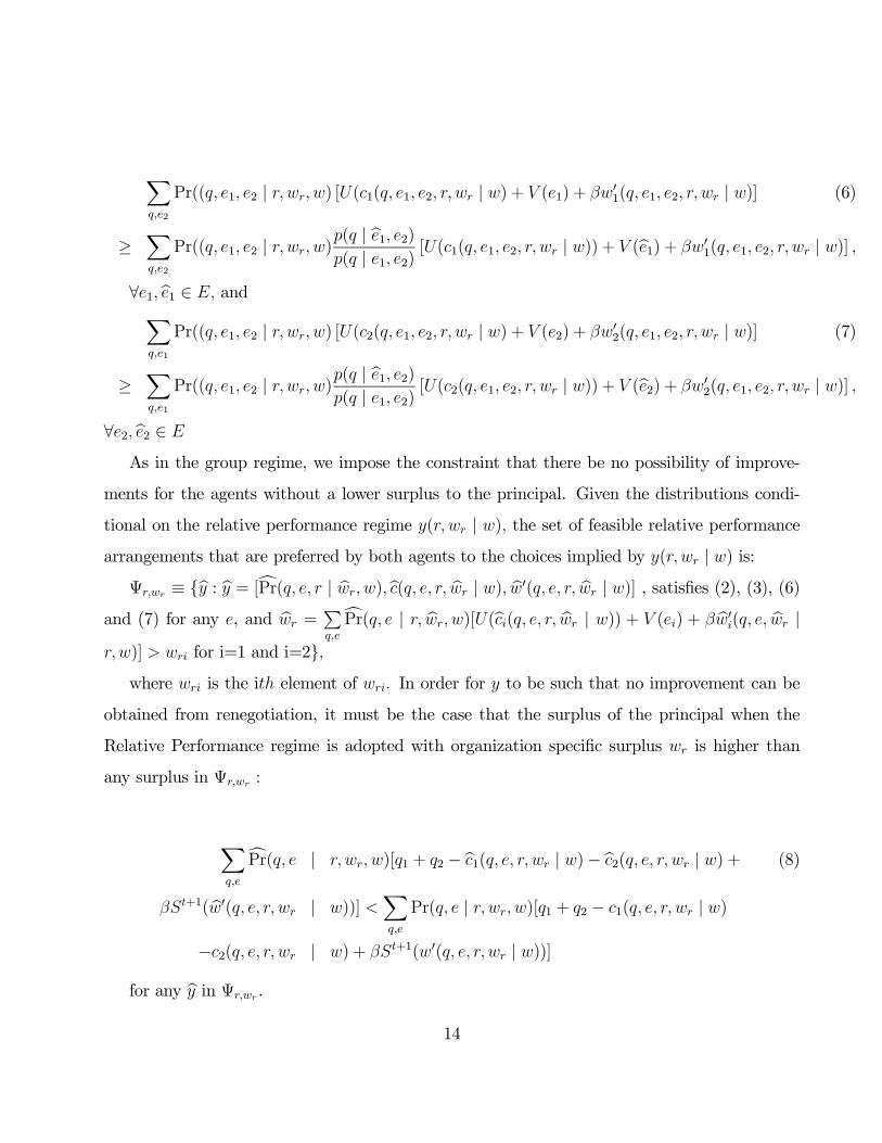
Xq,e2

Pr((q, e1, e2 | r, wr, w) [U(c1(q, e1, e2, r, wr | w) + V (e1) + βw01(q, e1, e2, r, wr | w)] (6)

≥Xq,e2

Pr((q, e1, e2 | r, wr, w)p(q | be1, e2)p(q | e1, e2) [U(c1(q, e1, e2, r, wr | w)) + V (be1) + βw01(q, e1, e2, r, wr | w)] ,

∀e1,be1 ∈ E, andXq,e1

Pr((q, e1, e2 | r, wr, w) [U(c2(q, e1, e2, r, wr | w) + V (e2) + βw02(q, e1, e2, r, wr | w)] (7)

≥Xq,e1

Pr((q, e1, e2 | r, wr, w)p(q | be1, e2)p(q | e1, e2) [U(c2(q, e1, e2, r, wr | w)) + V (be2) + βw02(q, e1, e2, r, wr | w)] ,

∀e2, be2 ∈ E

As in the group regime, we impose the constraint that there be no possibility of improve-

ments for the agents without a lower surplus to the principal. Given the distributions condi-

tional on the relative performance regime y(r, wr | w), the set of feasible relative performancearrangements that are preferred by both agents to the choices implied by y(r, wr | w) is:

Ψr,wr ≡ {by : by = [cPr(q, e, r | bwr, w),bc(q, e, r, bwr | w), bw0(q, e, r, bwr | w)] , satisfies (2), (3), (6)and (7) for any e, and bwr =

Pq,e

cPr(q, e | r, bwr, w)[U(bci(q, e, r, bwr | w)) + V (ei) + β bw0i(q, e, bwr |r, w)] > wri for i=1 and i=2},where wri is the ith element of wri. In order for y to be such that no improvement can be

obtained from renegotiation, it must be the case that the surplus of the principal when the

Relative Performance regime is adopted with organization specific surplus wr is higher than

any surplus in Ψr,wr :

Xq,e

cPr(q, e | r, wr, w)[q1 + q2 − bc1(q, e, r, wr | w)− bc2(q, e, r, wr | w) + (8)

βSt+1(bw0(q, e, r, wr | w))] <Xq,e

Pr(q, e | r, wr, w)[q1 + q2 − c1(q, e, r, wr | w)

−c2(q, e, r, wr | w) + βSt+1(w0(q, e, r, wr | w))]

for any by in Ψr,wr .

14

The Program The principal-agent problem at t is:

Program 15

St(w) ≡ max{Pr,c,w0}∈Y

Xq,e,wr

Pr(q, e, r, wr | w)[q1 + q2 − k − c1(q, e, r, wr | w)− (9)

c2(q, e, r, wr | w) + βSt+1(w0(q, e, r, wr | w))]+X

q,e,µ,wµ

Pr(q, e, µ, wµ | w)[q1 + q2 −

c1(q, e, µ, wµ | w)− c2(q, e, µ, wµ | w) + βSt+1(w0(q, e, µ, wµ | w))]

subject to the promise keeping constraintsXq,e,o,wo

Pr(q, e, o, wo | w)wo = w (10)

and for any bo in O and bwo in W 2,Xq,e

Pr(q, e, bo, bwo | w) [U(ci(q, e, bo, bwo | w)) + V (ei) + βw0i(q, e, bo, bwo | w)] = bwo (11)

Xq,e,o,wo

Pr(q, e, o, wo | w)= 1, and Pr(q, e, o, wo | w) ≥ 0 (12)

and (2),(4),(5),(6),(7) and (8). Notice from the objective function of Program 1 that an amount

k, corresponding to the cost to prevent collusion, is subtracted from the surplus whenever the

regime is relative performance. Program 1 defines the surplus function at t, St, given the

surplus function at t + 1, St+1. This characterizes a functional equation St = F (St+1). As in

Phelan and Townsend [21], a fixed point in this functional equation, S = F (S) is a solution for

an infinite period problem.

As we show now, this problem can be seen as a randomization between the choice of orga-

nization specific problems.

Definition 1 The surplus specific to organization o and utilities wo, So(wo) is the solution to

Program 1 without constraint (10) and with the additional constraint that6Pq,e

Pr(q, e, o, wo |

5There is an abuse of notation in using a sum here, since the space of wo is defined in a continuum. In any

event, the optimal solution has only a finite amount of values of wo with positive probability.6Using the notation of equation (1) Pr(o, e | w) ≡ Pr(o | w) · Pr(e | o,w).

15

w) = 1. fW o is the set of all values of wo for which this last program is defined. The policy graph

for organization o is ∆o(fW o) ≡ {[(fPr(q, e, o, wo | w),ec(q, e, o, wo | w), ew0(q, e, o, wo | w), wo] :fPr(q, e, o, wo | w),ec(q, e, o, wo | w), ew0(q, e, o, wo | w) solves the organization specific problemgiven wo in fW o}.

Proposition 1 S(w) can always be obtained as a randomization of organization specific sur-

pluses. More specifically: S(w) =Po,wo

Pr(o, wo | w)So(wo), and w =Po,wo

Pr(o, wo | w)wo.

Proof. Let y = {Pr(q, e, o, wo | w), c(q, e, o, wo | w), w0(q, e, o, wo | w)} be a solution to pro-gram 1. Suppose organization o with utilities wo is adopted with positive probability. Then,

yo,wo = {Pr(q, e, o, wo | w)/Pq,e

Pr(q, e, o, wo | w), c(q, e, o, wo | w), w0(q, e, o, wo | w)} must bea solution to the o and wospecific surplus maximization problem. Constraints (2) to (8) will

remain valid. Constraint (12) and (11)will also be valid. The choice yo,wo must maximize (9)

conditional on these constraints and onPq,e

Pr(q, e, o | w) = 1. If this were not true, another

object would maximize (9) conditional on these constraint and an improvement in the objective

of Program 1 would be possible by replacing the solution conditional on o and wo, y(o, wo | w),by this object, which would imply that y(w) is not optimal. The optimized value of (9) is

So(wo), and its contribution to the overall surplus of Program 1 is Pr(o, wo | w) · So(wo). So

if we consider all organizational forms and corresponding utilities with positive probability, we

have S(w) =Po,wo

Pr(o, wo | w) · So(wo). Note that the solution of the organization specific

problem incorporates randomization of recommended efforts given the organization. All incen-

tive constraints are conditional on the choice of organization, organization-specific utilities and

recommended effort. Any further randomization of effort is incorporated in the randomization

between organizations and organization-specific utilities. So, joint randomization of effort with

organization is allowed in this formulation

Notice from proposition 1 that for any w, the optimal arrangement can be obtained through

only a finite number of organizations and corresponding surplus levels.

We can impose if we wish, as an additional constraint to Program 1, that for any choice of

organization, the organization specific surplus wobe not smaller than a given outside option of

16

w: agents will only agree to join an organization that will give them an utility level that is not

lower than the one given by this outside option. Similarly, we can also impose that the surplus

of the principal obtained from agreements under any type of organization be not smaller than

an outside option S.

2.3 The Space of Promises and the Dynamics of the Model

The space on which the surplus function is defined is denoted by fW ⊆ W 2. This space will

depend on outside options of the agents and the principal and also on incentive compatibility.

Some utility pairs are not achievable by any regime. Suppose, for instance, that the utility

function has a lower bound or, without loss of generality, U(0) = 0. Then, the minimal level

of utility possible for each agent is that produced by zero consumption and high effort in all

periods. Even this level of utility cannot be sustained for both agents simultaneously. Incentives

for high effort require that rewards be given to at least one agent when high output is obtained.

At zero consumption to both agents, there is no incentive to make the high level of effort. The

space on which S is defined also incorporates potential lower bounds on the utility of each

agent. But if limc→0

U(c) = −∞ and agents have no outside option, the set fW is unbounded from

below. Also, if limc→∞

U(c) = ∞ and there is no outside option for the principal, the set fW is

unbounded from above.

Further, some regions of the utility map are reachable only by one regime. Under relative

performance, each individual needs incentives for high effort. Suppose U(0) = 0 and consump-

tion is always zero to some agent. His effort would then always be the least possible, el, and his

overall utility would be V (el)/(1− β). Any relative performance contracts must offer at least

this utility level. However, the group regimes is capable of sustaining arrangements with utility

as low as V (eh)/(1 − β) for (at most) one of the agents. That is, in the groups regime, it is

possible to impose high effort and zero consumption, for example when µi = 0, which provides

utility equal to V (eh)/(1− β) < V (el)/(1− β).

The solution to Program 1 determines the dynamic behavior for utility promises, and thus

17

of output, consumption and effort levels. The following results show that whenever high effort

is implemented by one of the agents, there is a positive probability that utility changes from

one period to the next. This is an extension of the result presented by Rogerson [25], that

in dynamic moral hazard problems, both current consumption and future utilities depend on

outputs. We extend Rogerson ’s proof to our model, in which the state of promises may be

bounded.

An important ingredient for this time variability of utility promises is that a Moral Hazard

problem actually exists, so that rewards depend on the realization of outputs. Again, however,

in a two agent setting where groups are allowed, high effort by one agent does not necessarily

imply the existence of a moral hazard problem. It is possible that the agent that is expected

to make high effort has zero Pareto weight inside a group. Lemma 1 below establishes that

a sufficiently high lower bound on promises rules out groups with zero Pareto weights, so

incentives for high effort always require some dependency of utilities on outputs.

Lemma 1 Suppose that a lower bound w is imposed for each organization o, so that wo > w.

In particular, suppose w > V (eh)/(1−β). Then, whenever at least one agent makes high effort,either consumption or future promises or both depend on outputs.

Proof. In the relative performance regime, agents have separate incentive constraints, so if

any agent makes high effort as in the premise, then that agent will require consumption and/or

promises to depend on output, otherwise his incentive constraint would not be valid. Let us

now consider the group regime. If µi = 0 for some agent i, the solution for a group will have

zero consumption, high effort and promises equal to w for i. Therefore, the current utility of i

will be V (eh) + βw. But by the premise of the Lemma, V (eh) + βw < w and this violates the

lower bound. So, if the group regime is chosen, µi > 0 for both agents. This implies that, even

if groups are chosen and one of the agents is expected to do low effort, consumption and (or)

promises must be dependent on outputs, otherwise the incentive constraint (4) would not be

satisfied..

18

The following Lemma is a version of the envelope theorem and presents some properties

relating the surplus function with the surplus obtained in each period. We use the following

notation: Z is the set of values of (q, e, o, wo) that are reached with positive probabilities in the

solution of Program 1, πz ≡ Pr(z) is the probability of state z ∈ Z. When z = (q, e, o, wo),

the notation cz denotes c(q, e, o, wo | w), w0z denotes w0(q, e, o, wo | w) and ez denotes e. The

notation uz ≡ U(cz) + V (ez) denotes the vector of current utilities (from current consumption

and effort), and s(u, e, q) = q1+ q2−U−1(u1− V (e1))−U−1(u2− V (e2)) is the current surplus

given current utility vector u, effort level e and output q.

Lemma 2 The following statements are valid for the solution of Program 1:

(a). If w is in the interior of fW , and for any z in Z consumption is positive, S(w) is differen-

tiable at w, and its gradient is given by:

S0(w) = E[su(uz, ez, qz)], (13)

where su(uz, ez, qz) is the gradient of s(u, e, q) with respect to u in state z.

(b). If w has some agent i at a lower bound of fW , or with consumption equal to zero in somestate z in Z.

Si+(w) ≥ E[su(uz, ez, qz)],

where Si+(w) is the right derivative of the surplus function with respect to the utility of agent i.

(c). If w has some agent i at an upper bound of fW with consumption positive for any z in Z,

S0i−(w) ≤ E[su(uz, ez, qz)],

where Si−(w) is the left derivative of the surplus function with respect to the utility of agent i.

Proof. We follow the Benveniste and Scheinkman theorem, as presented by Stokey and Lucas

[26]. The infinite periods surplus function S(w) is

S(w) =Xz∈Z

πz[s(uz, ez, qz) + βS(w0z)]

19

Since randomization is allowed between points with different utilities in all organizations, S is

concave.

(a). Adding an amount ε (a vector with two elements, that can be positive or negative) of utility

in every state through consumption would not change incentives for effort by agents and would

change instant utility by an amount ε. But from optimization and from the non-renegotiation

constraint, it must be the case that the surplus obtained in this way (increasing current utilities

by ε) is not higher than the surplus from the solution of Program 1 with initial promises w+ ε.

Therefore: Xz∈Z

πz[s(uz + ε, ez, qz) + βS(w0z)] ≤ S(w + ε) (14)

Since S(w) is concave and not lower than the expression on the left hand side of (14), it must

also be differentiable in the interior w, with its gradient equal to the gradient of the left-hand

side with respect to ε at ε = 0. Therefore:

S0(w) = E[su(uz, ez, qz)].

(b). In this case, it may not be possible to decrease utility of agent i by an equal amount in any

state using only consumption (either because this is a lower bound or because consumption is

zero in some state and cannot be decreased). But it is possible to increase the utility of agent

i only through consumption in any state, thus not affecting incentives. The resulting change

in surplus is given by the derivative of the left-hand side of (14) with respect to εi. From (14),

the change in optimal surplus of such an increase in utility cannot be smaller than this.

(c). In this case it is not possible to increase utility of both agents (since this is an upper

bound). But it is possible to decrease the utility of agent i by the same amount in every state

only through consumption, thus without affecting incentives. The resulting change in surplus

is the negative of the derivative of the left-hand side of (14)with respect to εi. From (14), the

change in optimal surplus of an decrease in utility cannot be smaller than this.

Note that statement (b) is relevant only for the case where fW has a lower bound (either

20

there is an outside option for the agents or U(0) has a finite value). Similarly, statement (c)

matters only for the case in where fW has an upper bound. These conditions are important to

prove Proposition 2.

Proposition 2 Suppose the conditions of Lemma 1 are valid. Suppose also that whenever one

agent is at an upper bound offW, consumption is always positive7. Then whenever w is such that

there is always at least one individual making high effort in the current period, the probability

that w0 6= w is positive.

Proof. We start from the case with the initial promise, w, in the interior offW and consumption

is positive in every state. Again, following Rogerson [25], incentives for efforts will not change

if, at any realization of uncertainty, z, consumption is subtracted in the current period so that

uz is replaced by uz−y and w0z is replaced by w0z+y/β,where y is also a vector with 2 elements.

The optimal choices for any z must thus solve at y = 0:

maxy

s(uz − y, ez, qz) + βS(w0z + y/β). (15)

If wz is in the interior of fW for any z in Z

su(uz, ez, qz) = S0(w0z). (16)

From Lemma 1, different levels of q imply different levels of either u (and thus consumption)

and or w0. But different levels of u imply different values for uz and thus, from (16) different

levels for w0z. This implies that, no matter the type of organization, for some level of output

(with probability not smaller than mine,q

p(q | e)) w0 will be different from w.

Let us now consider the case where consumption is equal to zero in some contingency or

the vector of initial promises, w has some agent i in a lower bound of fW . Suppose also thatincentives to i are given only through consumption, so w0zi = wzi for all z. From Lemma 2,

7Positive consumption in all contingencies is an endogenous result, a solution to the model, not a primitive

assumption. This is trivially true when limc→0 U(c) = −∞, but not necessarily true for the specifications weused. However, that consumption is always positive may be verified in numerical solutions.

21

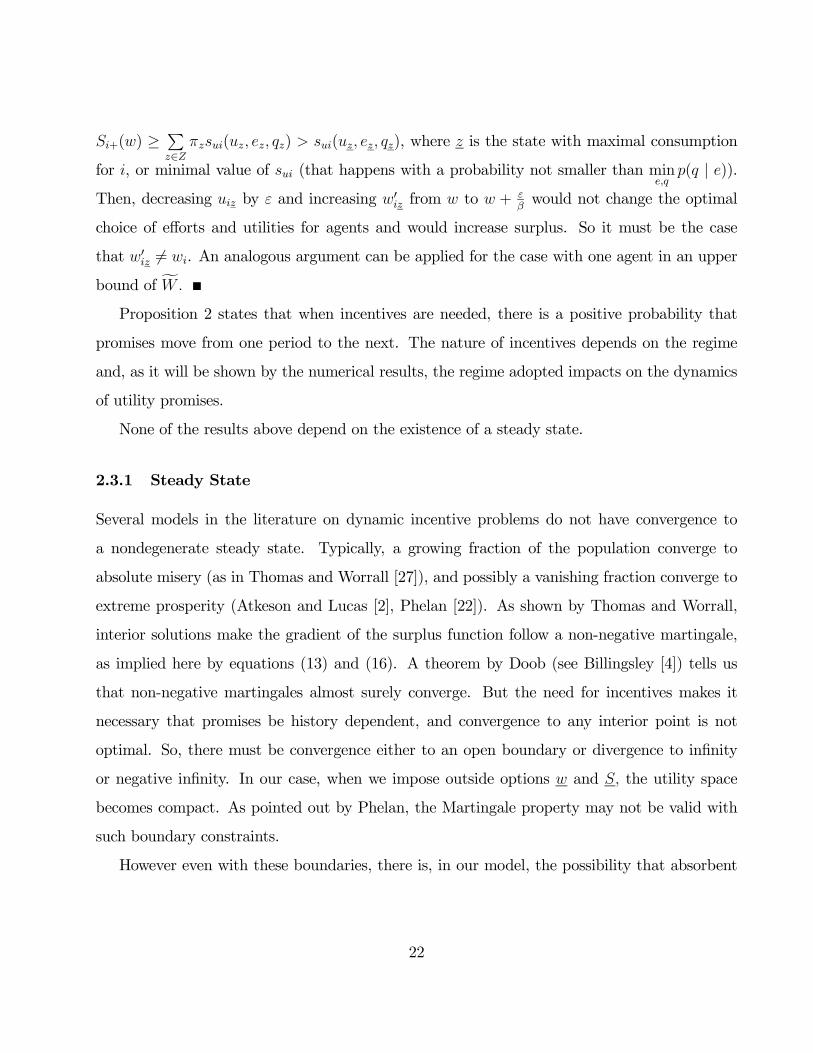
Si+(w) ≥Pz∈Z

πzsui(uz, ez, qz) > sui(uz, ez, qz), where z is the state with maximal consumption

for i, or minimal value of sui (that happens with a probability not smaller than mine,q

p(q | e)).Then, decreasing uiz by ε and increasing w0iz from w to w + ε

βwould not change the optimal

choice of efforts and utilities for agents and would increase surplus. So it must be the case

that w0iz 6= wi. An analogous argument can be applied for the case with one agent in an upper

bound of fW.

Proposition 2 states that when incentives are needed, there is a positive probability that

promises move from one period to the next. The nature of incentives depends on the regime

and, as it will be shown by the numerical results, the regime adopted impacts on the dynamics

of utility promises.

None of the results above depend on the existence of a steady state.

2.3.1 Steady State

Several models in the literature on dynamic incentive problems do not have convergence to

a nondegenerate steady state. Typically, a growing fraction of the population converge to

absolute misery (as in Thomas and Worrall [27]), and possibly a vanishing fraction converge to

extreme prosperity (Atkeson and Lucas [2], Phelan [22]). As shown by Thomas and Worrall,

interior solutions make the gradient of the surplus function follow a non-negative martingale,

as implied here by equations (13) and (16). A theorem by Doob (see Billingsley [4]) tells us

that non-negative martingales almost surely converge. But the need for incentives makes it

necessary that promises be history dependent, and convergence to any interior point is not

optimal. So, there must be convergence either to an open boundary or divergence to infinity

or negative infinity. In our case, when we impose outside options w and S, the utility space

becomes compact. As pointed out by Phelan, the Martingale property may not be valid with

such boundary constraints.

However even with these boundaries, there is, in our model, the possibility that absorbent

22

points exist in the feasible space of promises8. This may be the case if both individuals are

required to make low effort, which implies that consumption and promises do not need to

be output dependent. However, if the boundaries on promises are such that low effort is

never optimally recommended to both individuals, Proposition 2 guarantees that there are no

absorbent points.

The following results show that when high effort is implemented by at least one individual

in all points of fW there is no convergence in probability to any point of the compact set fW .Lemma 3 Suppose the surplus function S(w0) is well defined in a compact set fW. Suppose that

for some pair of real numbers w and S the additional constraints wo ≥ w for any o in O and

St(w) ≥ S are imposed in Program 1. Then, for any o ∈ O, if the set ∆o(fW o) of Definition 1

is not empty, it is compact.

Proof. It is straightforward to see that with the outside options w and S, the set ∆o(fW o), is

bounded for any organization o. We have to show that it is also closed. Indeed take a sequence

in ∆o(fW o), {Prn(q, e, o, wno | w), cn(q, e, o, wn

o | w), w0(q, e, o, wno | w), wn

o } converging to a limit{(fPr(q, e, o, ewo | w),ec(q, e, o, ewo | w), ew0(q, e, o, ewo | w), ewo}. The weak inequality constraints(2), (4), (6) ,(7) and the equality constraint (11)are clearly valid in this limit. It remains to

prove that the non-renegotiation constraint is valid for this limiting point.

Suppose first the regime is relative performance, so o = r and the non renegotiation constraint

is not valid in this limit. Then, there is some utility level w∗r > ewr that is feasible under

relative performance and has a surplus level S∗r ≥ eSr, where eSr is the surplus implied by{fPr(q, e, r, ewr | w),ec(q, e, r, ewr | w), ew0(q, e, r, ewr | w)}. Taking n = n high enough, wn

r < w∗r ,

so, by non-renegotiation, it must be true that the surplus associated with this element of the

sequence, Snr , is such that S

nr > S∗r ≥ eSr. There is some lottery between wn

r and w∗r that

would generate a utility pair wl > ewr and a surplus Sl > eSr. From the concavity of the utility

8In Thomas and Worrall [27], Atkeson and Lucas [2] and Phelan [22], shock dependence of promises is always

needed for incentive purposes. In the current model, this may not be the case if low effort is recommended for

both agents.

23

function and the surplus function, the utilities of these loteries can be generated by an object

yl = [Pr(q, e, r, wl | w),bc(q, e, r, wl | w), bw0(q, e, r, wl | w)] that does not have randomization ofconsumption and promises conditional on output and effort, that has a surplus bSr not smallerthan Sl, and still satisfies constraints (2), (3), (6) and (7). Thus, n high enough would have both

wnr < wl (so yl is an element of Ψr,wnr )and a surplus S

nr such that S

nr < bSr, which contradicts

non-renegotiation of points in the sequence. A similar proof applies to groups with Pareto

weights µ, focusing on the µ−weighted sum of utilities instead of the vector w directly.

Notice also that no matter the type of organization, the surplus in this limiting arrangement

must be optimal. If not, there is an arrangement with the same surplus and higher utility. It is

then possible depart from this last arrangement and increase the utility through consumption

in any contingency (such that incentives for efforts are never changed) and still have a surplus

higher than the elements of the sequence for high n enough. This would clearly violate non

renegotiation of points of the sequence.

Proposition 3 Suppose the conditions of Proposition 2 are valid, that the set fW is compact

and that in the solution to Program 1 there is always high effort by at least one agent. Then w

does not converge in probability to any point in fW .Proof. From Proposition 1, the policy graph ∆(fW ) = {[Pr(q, e, o, wo | w), c(q, e, o, wo |w), w0(q, e, o, wo | w), w] : Pr(q, e, o, wo | w), c(q, e, o, wo | w), w0(q, e, o, wo | w) solves Program1 given w} is given by optimal lotteries over elements of the compact sets ∆o(fW o)9. It must

thus be compact. We can define a continuous function from ∆(fW ) to < as f([Pr(q, e, o, wo |w), c(q, e, o, wo | w), w0(q, e, o, wo | w), w]) = max

(q,e,o,wo)|(w0(q, e, o, wo | w)− w) Pr(q, e, o, wo | w)| .

9Each element of ∆(fW ) is determined by choices of a lottery over organizations and the organization specific

utilities that maximize surplus conditional on overall expected utility values. The set from which these utilities

(and the corresponding policies) are taken, ∆o(fWo), are compact. So, the limit of a sequence of solutions will

be feasible. The maximizer of the problem is continuous in w (since randomization is alowed) so the surplus in

this limit will be optimal.

24

Since ∆(fW ) is compact, f has a minimum value d, that must be higher than zero from Propo-sition 2. So, the expected difference between w and and w0 is, at any point, not smaller than

some positive number, d, and the sequence does not converge.

Proposition 3 rules out convergence to a degenerate distribution and the existence of absorb-

ing points. It reassures us that when numerical computations find a non-degenerate distribution

of promises in the long run, the fact that this distribution is non-degenerate is not merely an

artifact of the discretization used in the computation. Notice that Proposition 3 depends on

at least one agent making high effort, which is a result and, not an assumption of the model.

But a numerical solution in which high effort is observed for every w is a good indication that

the dynamics have no absorbing points. Further assurance can be obtained by a comparison

between the surplus that is obtained by the numerical procedure to compute Program 1 for

each w and the surplus required to provide an utility pair w through low effort and constant

consumption over time.

3 Numerical Results

This section presents numerical solutions for Program 1. For computational purposes, we

discretised the values of consumption and promises and used linear programing, a method that

is convenient for problems with incentive constraints, where there may be randomization in the

optimal solution. We used grids of C with 18 elements, M with 101 elements, and W with 30

elements. We also broke the problem in several stages to deal with dimensionality problems.

The Appendix presents in more detail the procedure used to obtain these solutions.

In the numerical solutions, the set of possible effort levels and outputs per agent are respec-

tively E = {2, 6} and Q = {2, 20}. We use the following baseline specification: the utility ofconsumption and the disutility of effort are U(c) = c0.5 and V (e) = −e0.5, respectively. Thishas only a modest degree of risk aversion. The cost of blocking collusion, k, is equal to 0.3.

The discount rate β is 0.7 which is relatively low, but allows fast convergence to the infinite

25

period surplus function10. As in Prescott and Townsend [23], the technology P (q1, q2 | e1, e2),is given by the following table:

Table - I

q = (2, 2) q = (20, 2) q = (2, 20) q = (20, 20)

e = (2, 2) 0.6979 0.0021 0.0021 0.2979

e = (6, 2) 0.2991 0.4009 0.0009 0.2991

e = (2, 6) 0.2991 0.0009 0.4009 0.2991

e = (6, 6) 0.2979 0.0021 0.0021 0.6979

Notice that this matrix implies that outputs of agents are correlated11: if they do the same

amount of effort, it is very unlikely that their outputs will be different. We also assume a lower

bound on the utility of agents in each organization type of w = −5.812.10After 15 iterations, the maximum difference between St and St+1 was smaller than 10−5, and we assumed

that St was a reasonable approximation of the fixed point characterizing the infinite periods surplus function.11When both agents make low effort, the correlation coefficient of outputs is 0.9683, and when they make

high effort this coefficient is 0.99. The static literature on groups versus relative performance [e.g. Holmstrom

and Milgron [12] and Itoh [13] predicts that high correlation in outputs favors the relative performance regime.

Here we get some groups, nevertheless. A comprehensive review of the empirical literature on covariate risk

by Dercon [7] shows diverging results about the correlation between outputs. Some measures of covariate risk

such as rainfall, show considerably high correlation among plots inside villages, close to 1.0. However, it is

not obvious how to translate these results into the parameters of our model, since efforts are endogenous and

correlation of outputs depend on efforts.12This is smaller than the autarky utility for each agent. A possible interpretation for this lower bound smaller

than the autarky utility is that agents can move to autarky as an outside option but they have some punishment

when they do it, that could come from legal enforcement or social stigma. This particular lower bound has

been chosen to make the ergodic distribution of contracts more interesting. Without a lower bound on promised

utilities, the ergotic distribution has only group contracts at the axis region, with one of the agents having the

lower level of utilities possible. For the parametrization and the lower bound on promises used, the ergodic

distribution has significant probability of both assignment to the group regime and the relative performance

regime.

26

3.1 Solutions on the ex-ante utilities map

Expected Values for Ex-Ante Utility Pairs

Consumption of agent1 (c1)

-50

510

15

-5

0

5

100

10

20

30

40

W1W2

Promised Util.to agent1 (w01)

-50

510

15

-5

0

5

10-10

-5

0

5

10

15

W1W2

Effort of agent1 (e1)

-5 0 5 10 15-5

0

5

101

2

3

4

5

6

7

W1W2

Inside Group Pareto Weight of

Agent 1 if R.P. is not allowed (µ1)

-5 0 5 10

-4

-2

0

2

4

6

8

10

W1

W2

0.1

0.2

0.3

0.4

0.5

0.6

0.7

0.8

Figure 2

Figure 2 presents the expected values of effort, consumption and promised future utilities for

agent 1 at each ex-ante utility pair (in the horizontal axes) for the baseline case with infinite

periods. It also shows the expected value of the inside group Pareto weight of agent 1 when

the problem is restricted to the group regime. Notice that agent 1 tends to make the high

level of effort when his ex-ante utility is low, and the low level of effort when it is high. The

expected values of consumption and promised utility of agent 1 tend to increase with his level

of ex ante utility w1, except in the region of transition from high effort to low effort. Note also

that when the problem is restricted to groups, the Pareto weight of agent 1 tends to be higher

at the southeast of the main diagonal, where the utility of agent 1 is high compared with the

utility of agent 2.

27

Figure 3, shows the surplus that can be obtained under the relative performance regime

minus the group regime surplus for each utility pair13.

Surplus R.P. minus Surplus Groups

-50

5

-4-202468-5

-4

-3

-2

-1

0

1

2

W1W2

Figure 3

The horizontal axes represent ex-ante expected levels of utilities of the two agents. Notice

that for very low utility levels and high inequality with respect to utility, the group regime tends

to produce higher surpluses, so the net difference is negative. Note also that the fact that the

set of feasible utilities under groups is bigger than the feasible set under relative performance

is not the only potential advantage of groups: there is an area that is feasible under both

regimes but generates higher surplus under the Group Regime. This is true even if the cost

to avoid collusion k is equal to zero. When w1 = −5.1767 and w2 = 0.2253, for instance, the

difference between the surplus under groups and under relative performance is 1.04, bigger than

the fixed cost k = 0.3 of the relative performance regime. For intermediate utility levels and

low inequality, the relative performance regime produce higher surpluses.

Again, Figure 2 shows that for very high utility levels for agent 1, his optimal effort level is

low. A symmetric picture can be observed for agent 2. Thus, in the region where both agents

13These graphs are ploted for a subset of the promises space with utilities that can be generated by both

regimes. This happens for w1 and w2 bigger that -5.23.

28

have very high utilities (areas of low Surplus by the principal), no agent makes high effort. The

solution in this region resembles one without a moral hazard problem, and apart from the cost

to block collusion, k, the surplus under relative performance virtually equals the surplus under

groups. That is, the surplus under groups is higher than the surplus under relative performance

by an amount equal to k.

For Figures 2 and 3, no outside option for the principal is assumed14. In the following

results we impose a lower bound for the surplus of the principal, S = −315. With the limits onsurplus and utilities, one can verify that there is always one agent that makes high effort, and

incentives for effort are active in every point of the space of promises.

Figure 4 shows, as an example, the maximum surplus in each regime for different levels of

ex-ante expected utility for agent 1, w1, when the utility of agent 2 is fixed at 0.225316. Note

14Note however that we impose a grid of consumption with a maximum value of 40, so implicitly there is an

upper bound on utility and a lower bound on surplus from the fact that consumption can never be grater than

40 in each period. Evidently this is not low enough to rule out low effort.15The value of -3 for the outside option of the principal was chosen so that effort is always the maximal for

at least one agent, so promises and/or consumption must be output dependent.16Figure 3 is produced by the difference between the values expressed for a fixed w2 in Figure 4. Notice that

the graph in Figure 4 does not express the whole domain where the surplus function is well defined given w2,

but only a detail that makes the non convexity of the outer hull evident.

29

that the outer hull is not concave, so there may be randomization between regimes.

Surplus Under Both Regimes

w2Fixed at 0.2253

-5.5 -5 -4.5 -4 -3.5 -3 -2.5 -2 -1.5 -146

48

50

52

54

56

58

60

62

64

66

W1

S

Surplus GroupsSurplus R.P.

Figure 4

Regime dominance areas - Grey: No solution

Black: Prob. R.P.≥50% - White: Prob. Groups>50%

-4 -2 0 2 4 6 8 10 12

-4

-2

0

2

4

6

8

10

12

W1

W2

Figure 5

Figure 5 shows the areas, in the map of ex-ante utilities, w, where each regime dominates for

the baseline case. The black area represents the region where agents are assigned to the relative

performance regime with 50% or greater probability. In the white area, there is a probability

greater than 50% that they are assigned to the group regime. The grey areas are outsidefW,where the problem has no solution, either because surpluses are lower than S or because the

non renegotiation constraints are not valid, as in the extreme southwest of the utility maps17.

Notice again that the relative performance regime tends to dominate for intermediate levels of

utility and low levels of inequality. For most rays from the origin we would see a U shaped

frequency of groups.

3.2 Transitions between regimes

We have shown that when incentives for effort are needed, there is a positive probability that

w0 6= w. When this happens, regime change may occur. It may be the case that agents start

from an ex-ante utility pair w in the area of the utility map where one regime dominates, but

after outputs are realized, they move to an area where the other regime dominates. Figure

17In this area, the surplus function would be nondecreasing, which would violate non renegotiation.

30

6 presents the probability of transition between regimes at each point of the ex-ante utilities

map18. Notice that these transitions occur near the frontier between the areas in which each

regime dominates.

Probabilities of Transition Between Regimes

-4 -2 0 2 4 6 8 10 12

-4

-2

0

2

4

6

8

10

12

W1

W2

0.1

0.2

0.3

0.4

0.5

0.6

0.7

Figure 6

Tables II and III present a detailed description of the solution to the surplus maximization

problem for selected points in the utility map. They show the expected values of efforts,

consumption and promised future utilities conditional on output. Figures 7 and 8 show each

of these points as a white spot in the regime prevalence map. Table II and Figure 7 refer to

points where there is 100% of probability of Relative Performance, and Table III and Figure 8

to points where there is 100% of probability of group assignment.

Point one represents the utility pair (w1, w2) = (−3.5068,−3.5068). In this case, both agentshave 100% of probability of current assignment to the relative performance regime and the high

effort level is always recommended to both agents. When their outputs are the same, there

is no switching. But when the output of one agent is higher than the other, there is almost

100% probability of switching. In order to give incentives for high effort, the principal punishes

agents with low output. If outputs are unequal, the rewards to agents are also unequal. But

18A point in the utility map may have initial randomization between regimes. In this case, we calculate

the probability of transition by summing the probability of being initially in each regime multiplied by the

probability of transition conditional on the initial regime.

31

part of the reward is achieved with promised utilities, and unequal utilities tend to be produced

with a higher surplus under the group regime.

Table II – Expected Values Given Outputs for Selected Points With 100% R.P. Assignment Point 1: w=(-3.5068,-3.5068) Relative Performance Contracts-100% of total q1 q2 p(q1,q2) E(e1) E(e2) E(c1) E(c2) E(w1) E(w2) P(switch) ______________________________________________________________________________ 2.0000 2.0000 0.2979 6.0000 6.0000 1.5548 1.5548 -3.4941 -3.4941 0 20.0000 2.0000 0.0021 6.0000 6.0000 2.0000 0.4088 -2.8495 -5.7445 0.9933 2.0000 20.0000 0.0021 6.0000 6.0000 0.4088 2.0000 -5.7445 -2.8495 0.9933 20.0000 20.0000 0.6979 6.0000 6.0000 1.9318 1.9318 -3.3719 -3.3719 0 Point 2: w=(2.6085,2.6085) Relative Performance Contracts-100% of total q1 q2 p(q1,q2) E(e1) E(e2) E(c1) E(c2) E(w1) E(w2) P(switch) _____________________________________________________________________________ 2.0000 2.0000 0.2979 6.0000 6.0000 9.0000 9.0000 2.6950 2.6950 0 20.0000 2.0000 0.0021 6.0000 6.0000 8.7352 6.3611 3.7489 0.3684 0.3849 2.0000 20.0000 0.0021 6.0000 6.0000 6.3611 8.7352 0.3684 3.7489 0.3849 20.0000 20.0000 0.6979 6.0000 6.0000 9.0000 9.0000 3.0521 3.0521 0.3061 Point 3: w=(2.6085,-3.5068) Relative Performance Contracts-100% of total q1 q2 p(q1,q2) E(e1) E(e2) E(c1) E(c2) E(w1) E(w2) P(switch) ______________________________________________________________________________ 2.0000 2.0000 0.2979 6.0000 6.0000 9.0000 1.5612 2.4233 -3.4867 0.0129 20.0000 2.0000 0.0021 6.0000 6.0000 9.0000 0.3858 4.0016 -5.7959 0.9991 2.0000 20.0000 0.0021 6.0000 6.0000 6.2634 2.6897 0.1817 -3.1137 0 20.0000 20.0000 0.6979 6.0000 6.0000 9.0000 2.0682 3.1678 -3.4525 0.2917

Selected Starting Points With 100% of Relative Performance Assignment

Point 1 Point 2 Point 3

-4 -2 0 2 4 6 8 10 12

-4

-2

0

2

4

6

8

10

12

W1

W2

-4 -2 0 2 4 6 8 10 12

-4

-2

0

2

4

6

8

10

12

W1

W2

-4 -2 0 2 4 6 8 10 12

-4

-2

0

2

4

6

8

10

12

W1

W2

Figure 7

32

Table III – Expected Values Given Outputs for Selected Points With 100% Groups Point 4: w=(-1.2136,-5.8) Group Contracts-100% of total q1 q2 p(q1,q2) E(e1) E(e2) E(c1) E(c2) E(w1) E(w2) P(switch) ______________________________________________________________________________ 2.0000 2.0000 0.2979 6.0000 6.0000 1.8032 0.0821 -3.1078 -5.7899 0.0088 20.0000 2.0000 0.0021 6.0000 6.0000 3.4356 0.4824 -1.1698 -5.7899 0.0055 2.0000 20.0000 0.0021 6.0000 6.0000 2.2619 0.0821 -2.5383 -5.7899 0.0086 20.0000 20.0000 0.6979 6.0000 6.0000 5.2426 0.6666 -0.2218 - 5.5827 0.0855 Point 5: w=(7.1949,-0.44915) Group Contracts-100% of total q1 q2 p(q1,q2) E(e1) E(e2) E(c1) E(c2) E(w1) E(w2) P(switch) ____________________________________________________________________________ 2.0000 2.0000 0.2991 2.0000 6.0000 13.6650 4.7800 6.0908 -0.7910 0.0002 20.0000 2.0000 0.0009 2.0000 6.0000 13.6638 4.4468 6.1489 -1.1000 0.0004 2.0000 20.0000 0.4009 2.0000 6.0000 15.7363 5.9488 7.4344 -0.2345 0.0000 20.0000 20.0000 0.2991 2.0000 6.0000 13.6667 5.5378 6.8919 -0.4852 0.0000 Point 6: w=(5.6661,2.6085) Group Contracts-100% of total q1 q2 p(q1,q2) E(e1) E(e2) E(c1) E(c2) E(w1) E(w2) P(switch) ______________________________________________________________________________ 2.0000 2.0000 0.2991 2.0000 6.0000 9.4115 9.0000 4.1077 2.4903 0.5119 20.0000 2.0000 0.0009 2.0000 6.0000 10.6891 9.0000 3.6841 2.4903 0.6089 2.0000 20.0000 0.4009 2.0000 6.0000 13.6667 11.9464 5.8057 2.7311 0 20.0000 20.0000 0.2991 2.0000 6.0000 13.6667 9.5417 5.1694 2.7129 0

Selected Starting Points With 100% of Groups Assignment

Point 4 Point 5 Point 6

-4 -2 0 2 4 6 8 10 12

-4

-2

0

2

4

6

8

10

12

W1

W2

-4 -2 0 2 4 6 8 10 12

-4

-2

0

2

4

6

8

10

12

W1

W2

-4 -2 0 2 4 6 8 10 12

-4

-2

0

2

4

6

8

10

12

Figure 8

Point 2, utility pair (w1, w2) = (2.6085, 2.6085), is another example of 100% of probability of

assignment to the relative performance regime. As in the previous example, unequal outcomes

33

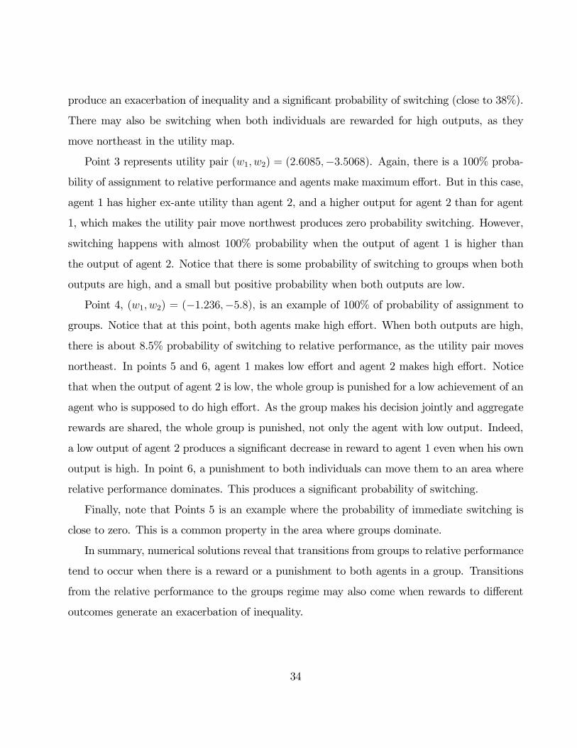
produce an exacerbation of inequality and a significant probability of switching (close to 38%).

There may also be switching when both individuals are rewarded for high outputs, as they

move northeast in the utility map.

Point 3 represents utility pair (w1, w2) = (2.6085,−3.5068). Again, there is a 100% proba-

bility of assignment to relative performance and agents make maximum effort. But in this case,

agent 1 has higher ex-ante utility than agent 2, and a higher output for agent 2 than for agent

1, which makes the utility pair move northwest produces zero probability switching. However,

switching happens with almost 100% probability when the output of agent 1 is higher than

the output of agent 2. Notice that there is some probability of switching to groups when both

outputs are high, and a small but positive probability when both outputs are low.

Point 4, (w1, w2) = (−1.236,−5.8), is an example of 100% of probability of assignment to

groups. Notice that at this point, both agents make high effort. When both outputs are high,

there is about 8.5% probability of switching to relative performance, as the utility pair moves

northeast. In points 5 and 6, agent 1 makes low effort and agent 2 makes high effort. Notice

that when the output of agent 2 is low, the whole group is punished for a low achievement of an

agent who is supposed to do high effort. As the group makes his decision jointly and aggregate

rewards are shared, the whole group is punished, not only the agent with low output. Indeed,

a low output of agent 2 produces a significant decrease in reward to agent 1 even when his own

output is high. In point 6, a punishment to both individuals can move them to an area where

relative performance dominates. This produces a significant probability of switching.

Finally, note that Points 5 is an example where the probability of immediate switching is

close to zero. This is a common property in the area where groups dominate.

In summary, numerical solutions reveal that transitions from groups to relative performance

tend to occur when there is a reward or a punishment to both agents in a group. Transitions

from the relative performance to the groups regime may also come when rewards to different

outcomes generate an exacerbation of inequality.

34

3.3 Steady State

Steady State Distribution of Promised Utility Pairs

59.47% probability of R.P. assignment

-50

510

-50

510

0

0.02

0.04

0.06

0.08

0.1

0.12

W1W2

Figure 9

The steady state19 distribution of utility pairs for the numerical solution to the baseline

specification is presented in figure 920. The long run distribution obtained has significant

presence of both the relative performance and the group regimes (59.47% probability of R.P.

assignment and 40.53% probability of Group assignment). The distribution concentrates in two

separate sets: one, in the central area of the picture, where relative performance dominates,

and another near the axes where group dominates. The area between these two sets has zero

19We verified that the choice of effort is always high for at least one agent.We also verified that the surplus

obtained by the numerical procedure with discretization is always higher than the surplus with low effort and

constant consumption. This reasures us that the existence of a nondegenerate long run distribution is not the

result of imperfections in the numerical method.20The optimal policy for problem 1 generates a transition matrix M such that, when M pre-multiplies a

vector with the probability distribution of w, the result is the probability distribution of w0. The steady state

distribution of promises is obtained by starting with some arbitrary distribution of w and successively pre-

multiplying it by M until the result converges to some vector, an invariant measure that corresponds to the

steady state distribution of promises.

35

or positive low mass in the steady state21. A possible explanation is that instead of promising

utilities in this area, it is preferable to randomize between a utility pair in the area where groups

dominate and another in the central area where relative performance dominates. As it can be

seen in Figure 4, the function max{Sr(w1, w2), Sg(w1, w2)} (where Sr(w1, w2) and Sg(w1, w2)

are the maximum surplus produced under the group and the relative performance regimes

respectively), is not concave (although both Sr(w1, w2) and Sg(w1, w2) are each concave) so the

optimal surplus may be obtained from a randomization of different points in the map.

3.4 Regime Volatility in the Utility Map

Figures 10 and 11 plot the probabilities of number of transitions over time22. More precisely,

they plot the probability that a pair starting at a given point switched regimes zero, one, two,

three, four or more than five times after a given amount of periods (in the horizontal axis).

We plotted these distributions for 1 to 100 periods. The paths described in Figure 10 all start

from the relative performance regime, but there is strong variability in organizational volatility.

Point 1 has strong regime persistence, but at points 2 and 3 it is very likely that after a few

periods at least one transition happens. Starting from point 2, the volatility stays high even

after the first transition. Indeed, the probability of more than 5 transitions increases rapidly.

This differs from the dynamics starting from point 3, that has a sharp decrease in the probability

21We sometimes found small positive probabilities in this area and it is possible that those result from

imperfections in the numerical results. On the other hand, the computed ergodic distribution is the same

regardless of the starting points and so these may play a genuine role. We conjectured, but have not proved,

that the ergodic distribution with the continuum is unique.22The procedure used to generate these distributions is the following: start with two state variables. A

transition matrix (that comes from the solution) determines the joint probability distribution of w01 and w02

(future promises) given the joint distribution of w1 and w2. We added another state variable: number of

transitions so far. The joint distribution of w1, w2 and the number of transitions until t determines its joint

distribution in t+1. For dimensional reasons, only up to 5 transitions are studied, so one of the possible states

is 5 transitions or more. Of course, over time, the probability that there is 5 or more transitions converge to 1

as in the steady state there is transit from one point to any other point in the support.

36

of no transitions in the first periods, but has relative stability after these first periods in the

sense that the probabilities of 0, 1, 2, 3 and 4 transitions decrease very slowly. The probability

of more than 5 transitions increases only slowly. After the first 10 periods, "survivors" that

did not switch in the initial periods tend to have strong persistence in the initial regime, and

economies that switch once in the early periods have relatively low volatility after this first

transition.

Figure 11 describe paths starting from the groups regime. Once again, there is considerable

variability in organizational volatility. In all points selected, there is a sharp decrease in the

probability of zero transitions in the initial periods. For point 4, however, after 20 periods there

is relatively high regime persistence both for those who switched once and for those that did

not switch in the initial periods. Point 5 has considerably higher regime volatility, but after

40 periods, there is still about 10% of probability of no transition, and the "survivors" in the

initial regime tend to have considerable persistence after 40 periods. Point 6 shows continuing

high volatility over time, and the probability of five or more transitions grows rapidly and is

higher than 80% after 50 periods.

3.5 Sensitivity to Alternative Parameter Specifications

This section show the response of the solution to alternative specifications of the model. We

solve the model for two alternative specifications of β and k. The results obtained suggest that

the general characteristics of the solution are not particular to the baseline parametrization we

used.

Figure 12 shows the difference between the surplus under relative performance and groups for

3 values of β. In all specifications the picture has a similar profile, with relative performance

producing higher surpluses for intermediate levels of utility and low levels of inequality. At

high β one does get the impression that the peak becomes more salient. However, there may

be numerical inaccuracies as β gets higher, as the computation of the infinite period solution

demands more iterations.

37

Figure 13, varying both β and k displays the dominance regions. Again these are quali-

tatively the same as in the baseline23. But note from Figure 13 that even when k, the fixed

cost of the relative performance, is equal to zero, there are areas where groups dominate and

areas where the relative performance regime dominates. But the area of group dominance in

the northeast does disappear.

Figure 14 shows the steady state distribution of utility pairs for all these specifications of

β and k. Notice that in all cases presented there is a positive probability of both groups and

relative performance. It follows that organization stability results will be similar qualitatively

but numerically distinct. The mass on the extremes seem to increase as β increases. The steady

state probability of relative performance assignments decreases as the cost to prevent collusion

k increases (naturally, as k is the fixed cost of relative performance assignment).

Figure 15 shows the probability of regime switching in each region of the utility map. In

every specification verified, there is some probability of switching near the frontier between the

areas in which regime dominate.

4 Conclusion

This paper presents a theory that generates coexistence of different contractual regimes, groups

versus relative performance, across local economies, even when the parametric specification

is fixed. We also solve the model numerically for several parametric specifications. These

numerical solutions generate both cross sectional and dynamic implications for observables.

The cross sectional results obtained by Prescott and Townsend [23] are maintained in our

formulation: the relative performance regime dominates for intermediate levels of wealth and

23Note that the space in which the problem is defined change as we change β. The minimum value possible

for utility when U(0) = 0 (as in our specifications) and the agents have no outside option is V (eh)/(1 − β),

that depends on β. We imposed an outside option for the agents roughly equal to 70% of this value in all

specifications, which results in w = −3.5 for β = 0.5 and w = −11.75 for β = 0.85. Notice that the maximumlevel of utility feasible given S also depends on β.

38

low inequality, the group regime for extremes in wealth and inequality (see Figure 13). However,

there may be randomization between regimes in optimal arrangements, so it is possible that local

economies with identical histories are assigned to different regimes. The model also generates

transitions between regimes. Intermediate levels of inequality are associated with a higher

probability of transition, although there are also transitions with low inequality for high and

low levels of wealth (see Figure 15). As it is shown in tables II and III, switches from relative

performance to groups can be accompanied by big shifts in inequality, while transitions from

groups to relative performance are related to changes in average wealth (promised utilities). We

compute long run distributions of wealth (utility), inequality and regime for local economies,

and both regimes are observed in these steady state distributions (Figure 14). The results show

much variation in regime volatility (figures 10 and 11) over the wealth (utility) / inequality

map. Different starting points, even in the same regime, produce highly different distributions

of number of transitions over time. In some areas there is a high probability of successive

transitions over time, while in others there is low probability of transition or one or a few

transitions tend to be followed by relative stability.

If we do not observe or infer the initial utility promise, as a starting point, the model still

has implications for observables, both the cross sectional distributions and the dynamic paths.

As in Karaivanov and Townsend [16], one can estimate the unobserved distribution of utility

starting points from the distributions of observables: consumption, output, and so on. But here

the regime may also be observable. The distribution of starting points can be parameterized

and estimated along with the parameters of technology and preferences, such as correlations

in return and risk aversion. The panel data are then determined by the evolution of utility

promises over time, something which comes from the model and depends on the parameters to

be estimated. The criterion for estimation could be a likelihood function or a mean square error

metric. This allows for measurement error and a variety of specifications of what is observable

39

by the econometrician.

Distribution Number of Transitions - Points With 100% Relative Perf. Assignment

Point 1 Point 2 Point 3

0 20 40 60 80 1000

0.1

0.2

0.3

0.4

0.5

0.6

0.7

0.8

0.9

1

Periods

zero transitionsone transitiontwo transitionsthree transitionsfour transitionsfive transitions or more

0 20 40 60 80 1000

0.1

0.2

0.3

0.4

0.5

0.6

0.7

0.8

0.9

1

Periods

zero transitionsone transitiontwo transitionsthree transitionsfour transitionsfive transitions or more

0 20 40 60 80 1000

0.1

0.2

0.3

0.4

0.5

0.6

0.7

0.8

0.9

1

Periods

zero transitionsone transitiontwo transitionsthree transitionsfour transitionsfive transitions or more

Figure 10

Distribution Number of Transitions - Points With 100% Group Assignment

Point 4 Point 5 Point 6

0 20 40 60 80 1000

0.1

0.2

0.3

0.4

0.5

0.6

0.7

0.8

0.9

1

Periods

zero transitionsone transitiontwo transitionsthree transitionsfour transitionsfive transitions or more

0 20 40 60 80 1000

0.1

0.2

0.3

0.4

0.5

0.6

0.7

0.8

0.9

1

Periods

zero transitionsone transitiontwo transitionsthree transitionsfour transitionsfive transitions or more

0 20 40 60 80 1000

0.1

0.2

0.3

0.4

0.5

0.6

0.7

0.8

0.9

1

Periods

zero transitionsone transitiontwo transitionsthree transitionsfour transitionsfive transitions or more

Figure 11

Surplus Under R. P.minus Surplus Under Groups

β = 0.5 β = 0.7 β = 0.85

-20

24

6

-20246-4

-3

-2

-1

0

1

2

W1W2

-50

5

-4-202468-5

-4

-3

-2

-1

0

1

2

W1W2

-100

1020

-10-505101520-1.5

-1

-0.5

0

0.5

1

1.5

W1W2

Figure 12

40

R.P. Dominates(Black) X Groups Dominate(White)X No solution (Grey)

β = 0.5 k = 0

-3 -2 -1 0 1 2 3 4 5 6 7

-3

-2

-1

0

1

2

3

4

5

6

7

W1

W2

-4 -2 0 2 4 6 8 10 12

-4

-2

0

2

4

6

8

10

12

W1

W2

β = 0.7 - Baseline k = 0.3 - Baseline

-4 -2 0 2 4 6 8 10 12

-4

-2

0

2

4

6

8

10

12

W1

W2

-4 -2 0 2 4 6 8 10 12

-4

-2

0

2

4

6

8

10

12

W1

W2

β = 0.85 k = 0.6

5 10 15 20 25 30

5

10

15

20

25

30

W1

W2

-4 -2 0 2 4 6 8 10 12

-4

-2

0

2

4

6

8

10

12

W1

W2

Figure 13

41

Steady State Distribution of Promised Utility Pairs

β = 0.5 (81.54%R.P.) k = 0 (73.93%R.P.)

-20

24

6

-20

24

60

0.02

0.04

0.06

0.08

0.1

0.12

W1W2-5

05

10

-50

510

0

0.05

0.1

0.15

W1W2

β = 0.7 (59.47%R.P.) - Baseline k = 0.3 (59.47%R.P.) - Baseline

-50

510

-50

510

0

0.02

0.04

0.06

0.08

0.1

0.12

W1W2-5

05

10

-50

510

0

0.02

0.04

0.06

0.08

0.1

0.12

W1W2

β = 0.85 (32.54%R.P.) k = 0.6 (32.91%R.P.)

-100

1020

-10

0

10

200

0.01

0.02

0.03

0.04

0.05

0.06

W1W2-5

05

10

-50

510

0

0.02

0.04

0.06

0.08

0.1

W1W2

−

Figure 14

42

Probabilies of Transition

β = 0.5 k = 0

-2 0 2 4 6

-3

-2

-1

0

1

2

3

4

5

6

7

W1

W2

0

0.1

0.2

0.3

0.4

0.5

0.6

-4 -2 0 2 4 6 8 10 12

-4

-2

0

2

4

6

8

10

12

W1

W2

0

0.1

0.2

0.3

0.4

0.5

β = 0.7 - Baseline k = 0.3 - Baseline

-4 -2 0 2 4 6 8 10 12

-4

-2

0

2

4

6

8

10

12

W1

W2

0.1

0.2

0.3

0.4

0.5

0.6

0.7

-4 -2 0 2 4 6 8 10 12

-4

-2

0

2

4

6

8

10

12

W1

W2

0.1

0.2

0.3

0.4

0.5

0.6

0.7

β = 0.85 k = 0.6

-10 -5 0 5 10 15 20

-10

-5

0

5

10

15

20

0

0.1

0.2

0.3

0.4

0.5

0.6

0.7

-4 -2 0 2 4 6 8 10 12

-4

-2

0

2

4

6

8

10

12

W1

W2

0

0.1

0.2

0.3

0.4

0.5

Figure 15

43

5 References

1. C. Ahlin and R. M. Townsend. “Selection into and across Credit Contracts:. Theory and

Field Research.” Forthcoming, Journal of Econometrics.

2. A.Atkeson and Robert E. Lucas, "On Efficient Distribution with Private Information",

Review of Economic Studies, (1992), 59(3), pp. 427-453.

3. Barkey, and van Rossen, (1997), "Networks of Contention: Villages and Regional Struc-

ture in the Seventeenth Century Ottoman Empire ", American Journal of Sociology,

102:5.

4. Billingsley, P. Probability and Measure, Willey, New York (1986).

5. R. Cavalcanti and N.Wallace, "Inside and Outside Money as Alternative Media of Ex-

change", Journal of Money, Credit and Banking, 31, no. 3, (1999). 443-457.

6. P.A. Chiappori, K. Samphantharak, S. Schulhofer-Wohl, and R.Townsend "Heterogeneity

and Risk Sharing in Thai villages",mimeo, (2006).

7. Dercon, S. and Krishnan, P. (2000), "In Sickness and Health: Risk Sharing within Holse-

holds in Rural Ethiopia", Journal of Political Economy, 108(4), 688-727.

8. S.Dercon, (2002), "Income Risk, Coping Strategies and Safety Nets", World Institute for

Development Economics Research, Discussion Paper No. 2002/22.

9. M. Fafchamps and S. Lund, "Risk-sharing networks in rural Philippines," Journal of

Development Economics, vol. 71(2), (2003) , 261-287

10. G.Genicot, and D. Ray, ”Endogenous Group Formation in Risk-Sharing. Arrangements“,

Review of Economic Studies, 70, (2003), 87-11

11. Grimard, F. "Household Consumption Smoothing through Ethnicities: Evidence from

Côte d’Ivoire" Journal of Development Economics, 1997. Vol. 53, 391-422.

44

12. B. Holmstrom and P. Milgron, "Regulating Trade Among Agents ", J. Inst. Theoret

Econ. 146 (1990), 85-105.

13. H. Itoh, "Coalitions, Incentives, and Risk Sharing", Journal of Economic Theory 60

(1993), 410-427.

14. M. Jackson and A. Watts,“Social Games: Matching and the Play of Finitely Repeated

Games”, mimeo,(2005).

15. A. Karaivanov and Townsend, R. M. (2006), "Firm Entry and Finance: Distinguishing

Information Regimes", mimeo, University of Chicago.

16. R. Kranton and Y Bramoullé, "Risk Sharing Networks," mimeo, (2005).

17. Leik, R.K. & Chalkey, M.A. (1997). On the stability of network relations under stress.

Social Networks, 19 (1), 63-74

18. D. C. Mills, "A model in which outside and inside money are essential ", mimeo, (2000).

19. Mueller, R. A. E., Prescott, E. S. and Sumner, D. A.(2002), "Hired Hooves: Transactions

in a South Indian Village Factor Market" . The Australian Journal of Agricultural and

Resource Economics, Vol. 46, pp. 233-255.

20. Murgai, R., P. Winters, E. Sadoulet and A. de Janvry "Localized and Incomplete Mutual

Insurance," Journal of Development Economics 67, (2002) 245-274.

21. C. P. Phelan and R. M. Townsend, "Computing Multi-Period, information-constrained

optima", Rev. Econ. Stud. 58 (1991), 853-881.

22. C. P. Phelan, "On the Long Run Implications of Repeated Moral Hazard" Journal of

Economic Theory, Volume 79, Issue 2, (1998), Pages 174-191

45

23. E. S. Prescott and R.A. Townsend, "Collective Organizations Versus Relative Performance

Contracts: Inequality, Risk Sharing and Moral Hazard ", J. Econ Theory 103 (2002) 282-

310.

24. R. T. S. Ramakrishnan and A. V. Thankor, "Cooperation Versus Competition in Agency",

J. Law. Econ. Organ. 7 (1991), 248-283.

25. Rogerson, W. P., "Repeated Moral Hazard", Econometrica, Vol. 53(1), (1985), pp. 69-96.

26. N. Stokey and Lucas, R. E., Recursive Methods in Economics, Harvard University Press,

Cambridge, MA, (1996).

27. Thomas, J and T. Worrall (1990), "Income Flutuations and Asymmetric Information: An

Example of a Repeated Principal-Agent Problem.", Journal of Economic Theory, 51(2),

pp. 367-390.

28. R. Townsend, "Risk and Insurance in Village India", Econometrica, 62(3), (1994), 539-

591.

29. R. M. Townsend and R. A. E. Mueller, "Mechanism Design and Village Economies:

Credit to Tenancy to Cropping Groups", Rev. Econ. Dynam. (1998), 119-172.

46

6 Appendix A - Reformulated discretized version and

Numerical Procedure

In this appendix we present a discretized version of the mechanism design problem, which is

important for the numerical methods used. This requires that we utilize a grid for consumption

and promised utilities. The choice of consumption and promises are thus given by a lottery

on the elements of these grids. Given a curse of dimensionality that may arise from the mere

discretization of the problem as described in Program 1, we also break the problem in several

stages.

One fact that is useful to reduce the dimension of the problem is that the distributions

of consumption values , c1and c2, and promises w01 and w02 are relevant in the decisions of

agents or groups only through their effects on the composite terms U(c1) + βw01 ≡ v1 and

U(c2) + βw02 ≡ v2. These terms represent the utility that comes from both consumption and

future contracts. Throughout the remainder of this appendix, we call v ≡ (v1, v2) the interimutility vector. In order to diminish the size of the decision vector, we formulate the moral

hazard problem making v a decision variable, not c and w separately.

This strategy requires another maximization stage in any period t. For a fixed vector (v1, v2),

different distributions of c and w imply different expected values for the ex-post (after output

is realized) surplus −c1−c2+ 11+r[St+1(w01, w

02)] , denoted eSt. In order to determine the cost (or

benefit) of offering an utility pair (v1, v2), we need to solve the problem of choosing vectors of

consumption and promised future utilities that maximize the expected value of eSt conditional

on (v1, v2).

Following the formulation described in Proposition 1, we first solve the problem assuming

that only the relative performance regime is available, and then solve it using only the group

regime. From these programs we construct a grid of surplus maximizing contracts for each

regime. The general program in which both regimes are allowed is then solved by randomization

of the elements of these grids. This procedure of solving the problem separately for each

47

regime makes computation easier (we solve smaller programs) and allows us to compare the

performance of the regimes in each area of the utility pairs map.

Figure A

The structure of the reformulated problem is illustrated in figure A. At the beginning of any

period, a level of promises w is taken as given . In order to deliver these promises, an optimal

arrangement defines a joint distribution of the regime assignment and utility pairs specific

to the regime (ew1, ew2) . These utility pairs are delivered by an assignment of, first internalPareto weights µ if the regime is groups, then levels of effort (e), and finally interim utilities(v)

conditional on outputs (q). These interim utilities are delivered by current consumption (c)

and promises for future periods (w0).

The optimal policy by the principal involves 3 maximization stages, that can be solved

backward. In a first stage (the last one chronologically), the principal choses the distribution of

consumption c and promisesw0 that produce each interim utility pair with maximal surplus, thus

defining eSt(v). Notice that consumption c and promises w0 are defined from a randomization of

elements in a grid. In another stage, that depends on the regime adopted, the principal takes the

interim surplus function as given, and chooses the joint distribution of internal Pareto weights

(if the regime is group), efforts, output and interim promises that maximizes surplus subject

48

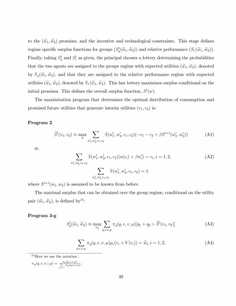
to the (ew1, ew2) promises, and the incentive and technological constraints. This stage definesregime specific surplus functions for groups (St

g(ew1, ew2)) and relative performance (Sr(ew1, ew2)).Finally, taking St

g and Str as given, the principal chooses a lottery determining the probabilities

that the two agents are assigned to the groups regime with expected utilities (ew1, ew2), denotedby eπg(ew1, ew2), and that they are assigned to the relative performance regime with expectedutilities (ew1, ew2), denoted by eπr(ew1, ew2). This last lottery maximizes surplus conditional on theinitial promises. This defines the overall surplus function, St(w).

The maximization program that determines the optimal distribution of consumption and

promised future utilities that generate interim utilities (v1, v2) is:

Program 2

eSt(v1, v2) ≡ maxeπX

w01,w02,c1,c2

eπ(w01, w02, c1, c2)(−c1 − c2 + βSt+1(w01, w02)) (A1)

st. Xw01,w

02,c1,c2

eπ(w01, w02, c1, c2)(u(ci) + βw0i) = vi, i = 1, 2, (A2)

Xw01,w

02,c1,c2

eπ(w01, w02, c1, c2) = 1.where St+1(w1, w2) is assumed to be known from before.

The maximal surplus that can be obtained over the group regime, conditional on the utility

pair (ew1, ew2), is defined by24:Program 3-g

Stg( ew1, ew2) ≡ max

πg

Xq,e,v,µ

πg(q, e, v, µ)[q1 + q2 + eSt(v1, v2)] (A3)

Xq,e,v,µ

πg(q, e, v, µ)µi(vi + V (ei)) = ewi, i = 1, 2, (A4)

24Here we use the notation :

πg(q, e, v | µ) = πg(q,e,v,µ)Pq,e,v

πg(q,e,v,µ).

49

Xq,v

πg(q, e, v | µ)Xi

µi[vi + V (ei)] ≥Xq,v

πg(q, e, v | µ)p(q | be)p(q | e)

Xi

µi[vi + V (bei)],∀e, be, µ. (A5)Xv

πg(bq, be, v | µ) = p(bq | be)Xv,q

πg(q, be, v | µ), ∀bq, be, µ (A6)

πg ≥ 0 andXq,e,v

πtg(q, e, v, µ) = 1. (A7)

Xq,e,v

πg(q, e, v | µ)hq1 + q2 − eSt(v1, v2)

i(A8)

≥Xq,e,v

bπ(q, e, v | µ) hq1 + q2 − eSt(v1, v2)i

for any µ and any bπ in the set:eΨr(µ, πg) ≡ {bπ(q, e, v | µ) : bπ is positive, sums to 1 and satisfies (A5) and (A6) for anye given µ and

Pq,e,v

bπ(q, e, v | µ)Pi

µi [vi + V (ei)] ≥ wµ(πg)}, where wµ(πg) =Pq,v

πg(q, e, v |µ)Pi

µi [vi + V (ei)]

The analogous program that generates the maximum surplus under the group regime is:

program 3-r

Str(ew1, ew2) ≡ max

πr

Xq,e,v

πr(q, e, v)[q1 + q2 + eSt(v1, v2)] (A9)

st. Xq,e,v

πr(q, e, v)(vi + V (ei)) = ewi, i = 1, 2, (A10)

Xq,v

πr(q, e, v)[vi + V (ei)] ≥Xq,v

πr(q, e, v)p(q | bei, e−i)p(q | e) [vi + V (bei)], ∀ei, bei, i = 1, 2, (A11)

Xv

πr(bq, be, v) = p(bq | be)Xv,q

πr(q, be, v), ∀bq, be, (A12)

50

Xq,e,v

πr(q, e, v) = 1. (A13)

Xq,e,v

πr(q, e, v)hq1 + q2 − eSt(v1, v2)

i(A14)

≥Xq,e,v

bπ(q, e, v) hq1 + q2 − eSt(v1, v2)i

for any bπ in the set:eΨr(πr) ≡ {bπ(q, e, v) : bπ is positive, sums to one and satisfies (A11) and (A12) for any e andi, and

Pq,e,v

bπ(q, e, v) [vi + βw0i] ≥ wi,r(πr) for i=1,2}, where

wi,r(πr) =Xq,ei,v

πr(q, e, v) [vi + V (ei)]

With the surplus functions in for groups and relative performance, we are finally able to

provide an approximation to the surplus function at t, St(w1, w2). The surplus is approximated

by:

Program 4

St(w1, w2) ' maxeπg ,eπrXew1, ew2

eπg(ew1, ew2)Stg(ew1, ew2) (A15)

+Xew1, ew2

eπr(ew1, ew2)(Str(ew1, ew2)− k),

st.

wi =Xew1, ew2

ewi (eπg(ew1, ew2) + eπr(ew1, ew2)) , (A16)

i = 1, 2. Xew1, ew2

(eπg(ew1, ew2) + eπr(ew1, ew2)) = 1, eπg, eπr ≥ 0, (A17)

where Sg(ew1, ew2) and Sr(ew1, ew2) are defined in problems 3-r and 3-g.With fine enough grids for ew1, ew2, v1, and v2, the solution of program 4 is a good ap-

proximation to the solution of Program 1. The proposed reformulation, with interim utilities,

51

reduce considerably the dimension of the linear programming problems. Suppose again that Q,

E, C, W and M have, respectively, 2, 2, 18, 30 and 101 elements, and that we adopt a grid

of interim utilities with 26 elements. The decision vector in Program 2 has 291,600 elements

and the problem has 3 constraints, Program 3-r has a choice vector with 10,816 elements and

has 21 constraints (excluding the non-renegotiation constraint that, as pointed out below, is

not directly used in the computation). In contrast, the decision vector of the program for the

relative performance regime without interim utilities with the same grids would have 4,665,600

elements and the problem would have the same 21 constraints. This last problem requires

considerably higher computational capacity than the subprograms mentioned above.

In order to obtain an approximation of Sg(ew1, ew2), we use the fact that , from (A8), any

arrangement for a group conditional on any µ, must maximize the sum of µ-weighted utilities

conditional on an incentive constraint (A5)(that depend on µ), the technological constraint

(A6) and the surplus level obtained under µ. In our numerical procedure for groups, we first

take a grid of 101 values of µ and 52 of values surplus level. Then, for each point in the grid,

we use a linear program to maximize, by the choice of a lottery πg,µ, the µ-weighted sum of

utilities (P

q,e,v πg,µ(q, e, v)(vi + V (ei))) conditional on incentive and technological constraints

like (A5) and (A6) and the surplus level in the gridpoint. The solution for each point of this grid

determines a triple with surplus level, utility for agent 1 and utility of agent 2. We depart from

the triples thus generated to compute an approximation of the solution to program 3g. This

is obtained from an optimal randomization (that maximizes surplus conditional on utilities) of

the triples that are obtained in the grid of Pareto weights and surplus levels.

In the relative performance computations, we initially do not use the non-renegotiation

constraint. We initially solve the problem with a weak inequality in the promise keeping con-

straint (we maximize surplus conditional on the minimal levels for utilities)25. We compute the

problem with this formulation until the surplus function thus obtained converges. This will

25In our numerical experiments, the use of inequality constraints was faster and more stable than the use of

equality constraints.

52

result in points where an increase in utility under relative performance does not imply a lower

surplus, and thus improvements from renegotiation are possible. We suppress these areas from

the choice space and recompute the problem. If a new area of noincreasing surplus is again

observed, we remove it once more. This problem is recomputed until convergence to a constant

space of choice is obtained. Similar procedure is used in the upper bound of the utility space.

We start without imposing a lower bound on surplus, until the surplus function converges.

Then we remove the area with surplus lower than the outside option from the space of promises

and recompute the problem. If a new area with surplus lower than the lower bound emerges,

we remove it form the space os promises. This process runs until convergence to a constant

space of promises is reached.26

26This procedure produced fast convergence to a constant discrete grid of feasible promises, normally with

less than 5 iterations.

53