TI 2015-066/VI Tinbergen Institute Discussion Paper

Inflation, Endogenous Market Segmentation and the Term Structure of Interest Rates Casper de Vries Xuedong Wang

Erasmus School of Economics, Erasmus University Rotterdam, and Tinbergen Institute, the Netherlands.

Tinbergen Institute is the graduate school and research institute in economics of Erasmus University Rotterdam, the University of Amsterdam and VU University Amsterdam. More TI discussion papers can be downloaded at http://www.tinbergen.nl Tinbergen Institute has two locations: Tinbergen Institute Amsterdam Gustav Mahlerplein 117 1082 MS Amsterdam The Netherlands Tel.: +31(0)20 525 1600 Tinbergen Institute Rotterdam Burg. Oudlaan 50 3062 PA Rotterdam The Netherlands Tel.: +31(0)10 408 8900 Fax: +31(0)10 408 9031

Duisenberg school of finance is a collaboration of the Dutch financial sector and universities, with the ambition to support innovative research and offer top quality academic education in core areas of finance.

DSF research papers can be downloaded at: http://www.dsf.nl/ Duisenberg school of finance Gustav Mahlerplein 117 1082 MS Amsterdam The Netherlands Tel.: +31(0)20 525 8579

Inflation, Endogenous Market Segmentation and theTerm Structure of Interest Rates

Casper G. de Vries∗ Xuedong Wang†

May 18, 2015

Abstract

The term structure of interest rates does not adhere to the expectations hy-

pothesis, possibly due to a risk premium. We consider the implications of a risk

premium that arises from endogenous market segmentation driven by variable

inflation rates. In the absence of autocorrelation in inflation, the risk premium

is constant. If inflation is correlated, however, the risk premium becomes time

varying and we can rationalize the failure of the expectations hypothesis. In-

direct empirical tests of the model’s implications are provided.

JEL Classification: E43, G12

Keywords: Expectations hypothesis; Term structure; Time-Varying Risk Premia;

Segmented markets; Inflation

1 Introduction

The expectations hypothesis (EH) of the yield curve of interest rates holds that the

n-period yield is a weighted average of the m period yield, m < n, and the expected

(n−m)-period yield. Empirical work has consistently rejected this linear relationship. The

failure of the EH in term structure of the yield curve was first observed by Fama and Bliss

(1987). Many other papers have subsequently documented the same result of Famma, see

∗Erasmus School of Economics, Erasmus University Rotterdam and Chapman University†Corresponding author: Erasmus School of Economics, Erasmus University Rotterdam and Tinbergen

Institute, P.O. Box 1738, 3000 DR, Rotterdam, The Netherlands. Email: xwang@ese.eur.nl. We are grateful toWouter den Haan who commented on a first draft of the paper.

1

e.g. Campbell and Shiller (1991), Hardouvelis (1994), Gerlach and Smets (1997), Bekaert

and Hodrick (2001) to name a few.

Currently, the main explanation for the rejection of EH in the term structure is the

existence of time varying risk premia.1 Due to the rather small variations in aggregate

consumption, a representative agent model with a standard utility function cannot gener-

ate large and variable risk premia. For this reason, the explanations based on such frame-

work, including the work of Backus, Gregory, and Zin (1989), Donaldson, Johnsen, and

Mehra (1990), den Haan (1995) and Bekaert, Hodrick, and Marshall (1997), encounter dif-

ficulties. The time varying risk premia have been explained by means of habit formation

in preference functions, see e.g. Brandt and Wang (2003), Wachter (2006), or by means of

the Epstein-Zin recursive recursive utility function, as in Bansal and Shaliastovich (2007),

and Rudebusch and Swanson (2012). A different avenue has been followed by Buraschi

and Jiltsov (2005), who rely on a tax wedge.

There is a smaller but growing literature that explains time varying risk premia from

endogenous market segmentation. Limited participation implies that a subset of the pop-

ulation is responsible for the adjustments in financial markets. This generates larger risk

premia than representative agent models in which everyone participates in (complete) fi-

nancial markets. In addition to the exogenous assumption that there are different types of

households, there are two effective ways to generate endogenous segmentation between

households.

One assumption is that financial markets are complete coupled with limited enforce-

ment of financial contracts.2 Seppala (2004) compares the real term structure under the no

friction Lucas economy (see Lucas (1978)) and the limited risk-sharing Alvarez-Jermann

economy (Alvarez and Jermann (2001)). Seppala shows that “only the model with limited

risk-sharing can generate enough variation in the term premia to account for the rejections

of expectations hypothesis” (Seppala (2004), p1510).

The second avenue is the segmented market approach. An endogenous market seg-

mentation model was developed by Alvarez, Atkeson, and Kehoe (2002) and (2009). In Al-

1Several other explanations have been offered. For example, Bekaert, Hodrick, and Marshall (2001) refer tothe peso problem. Bansal and Zhou (2002) use a regime shifting model, while Sinha (2009) considers learningbehavior.

2The idea of limited contract enforceability was first used by Kehoe and Levine (1993) for investigating thebehavior of asset markets. Later it was used by Alvarez and Jermann (2001) for examining the implications ofasset pricing and by Kehoe and Perri (2002) for exploring the implications of the international business cycle.

2

varez, Atkeson, and Kehoe (2009), the endogenously segmented market model generates

sufficient large variation of the time-varying risk premia to resolve the forward premium

puzzle of exchange rates.

Inspired by the model of Alvarez, Atkeson, and Kehoe (2009), we address the expec-

tations puzzle with an endogenously segmented market model. We solve the model with

correlated inflation and show that this is necessary for rejection of the EH. The intuition

is as follows. In the absence of autocorrelation in inflation, the risk premium is constant.

This is unimportant in the two period model of Alvarez, Atkeson, and Kehoe (2009). But

to explain the the yield curve, one needs a multiperiod model in which pricing kernels are

correlated. If inflation is correlated, however, the risk premium becomes time varying and

we can rationalize the failure of the expectations hypothesis. We also provide a test for the

model by relating the size of the bias to the amount of autocorrelation and the level of the

variance of the money supply shocks.

The remainder of the paper is organized as follows. Section 2 reviews the empirical

tests for the EH in term structure. Section 3 gives a concise description of the model.

Section 4 provides the theoretical proof that the consumption-based model can reslove the

expectations puzzle. Section 5 offers numerical backing. Section 6 presents the empirical

evidence for our results. Section 7 concludes.

2 Empirical Evidence Review

Using postwar U.S. bond yields, Campbell and Shiller (1991) show the values of β in

regressions like

yt+m,n−m − yt,n = const+ βn,mm

n−m(yt,n − yt,m) + error

are negative and increase in absolute value with maturity n for almost any combination

of maturities between one month and ten years. The EH holds that β = 1. This evidence

constitutes the expectations puzzle of the term structure, first documented by Fama and

Bliss (1987) and Campbell and Shiller (1991).3 In addition to nominal yields, the real yields

also reject the EH, see Bansal and Shaliastovich (2007) and Sinha (2009).

3A related rejection of the EH exists in the foreign exchange markets. This was first documented by Fama(1984) and is usually referred to as the forward premium puzzle.

3

Backus, Foresi, Mozumdar, and Wu (2001) and Buraschi and Jiltsov (2005) use U.S.

data and obtain results similar to Campbell and Shiller (1991). Empirical tests conduct-

ed on interest rates outside the US, however, often show that the EH cannot be rejected

at multiple horizons.4 More importantly, empirical results show that yields of long-term

maturities are more likely to violate the EH than yields of short-term maturities. Hardou-

velis (1994) tests the long-term (10-year) and short-term (three-month) bond yields in G7

countries. When the long-term yields are used, five out the seven countries give nega-

tive β. However, for the short-term yields, all countries have a positive β, though all of

these are lower than 1. Gerlach and Smets (1997) test the EH with 1-, 3-, 6- and 12-month

Euro-rates. Their results show that the EH cannot be rejected for 35 cases out of the total

51 cases. Longstaff (2000) tested the expectations hypothesis at the extreme short end of

the term structure using overnight, weekly, and monthly repo rates. His results show the

expectations hypothesis cannot be rejected at any maturity level.

Table 1 shows the results of our test using Euro-rates for the currencies of 17 countries.

Our results also show that the negative βn,m is not universal. The empirical values of β

are either smaller or larger than unity. For example, all the values of βn,m for French franc

rates are larger than unity and increase in n. So the expectations hypothesis is rejected

in two directions and one would also like to be able to account for this. Moreover, the

decreasing trend of β in n is observed in only a few countries, such as Australia and the

U.S. While for most countries, this trend is absent.

3 The Model with Segmented Markets

The baseline model that we use is the same with that of Alvarez, Atkeson, and Kehoe

(2009). This section provides a concise description of the model.

In the economy there is an asset market and a goods market. Households can buy

and sell government bonds in the asset market. The Government injects money in the

asset market by paying the maturing bonds. This determines the money growth rate µt.

In each period, the shock to money growth is the only source of uncertainty in this econ-

omy. At the end of each period, each household receives the same real endowment y.

4For the empirical test of EH for other countries, see Hardouvelis (1994), Evans and Lewis (1994) Gerlachand Smets (1997), Longstaff (2000), Dominguez and Novales (2000), Bekaert and Hodrick (2001), and Jongen,Verschoor, and Wolff (2011) et al.

4

Households sell their endowment at the current price level Pt to obtain money Pty and

transfer money to the next period for consumption in the goods market or for buying

bonds in the asset market. Money can be transferred between the goods market and the

asset market. Households who transfer money between the two markets have to pay a

real transfer cost γ. Besides the traditional interpretation for such a cost as the brokerage

fee, the bid-ask spread and the transaction tax, the literature explores more motives for

this cost. Chatterjee and Corbae (1992) view the transfer cost as a cost involved in writing

enforceable private debt contracts. Reis (2006) and Alvarez, Guiso, and Lippi (2012) con-

sider the costs of acquiring, absorbing and processing information. Gust and Lopez-Salido

(2014) interpret the presence of the transfer cost as reflecting time spent on the activities

of re-optimizing and responding to new information, and the human inertia of sticking

to a predetermined plan. Thus one can consider the transfer cost as the aggregate effect

of all kinds of frictions which can be tangible or intangible. The value of γ varies across

households with a distribution F (γ) and density f(γ).

There is no storage technology available in the economy except for money, so the en-

dowment y of each period has to be consumed within the same period. The consumption

of households is subject to the cash-in-advance constraint and the transition law. In period

t, given state st,

c(st, γ) =P (st−1)y

P (st)+ x(st, γ)z(st, γ) (3.1)

The resource constraint is given by

∫ [c(st, γ) + γz(st, γ)

]f(γ)dγ = y (3.2)

where c(st, γ) is the consumption of a household in period t and x(st, γ) is the real balance

that the household chooses to transfer between the two markets. If the value of x(st, γ) is

positive, it means that money is transferred from the asset market into the goods market,

and vice versa. The indicator variable z(st, γ) is equal to 0 if x(st, γ) is 0, otherwise, it is

equal to 1.

It is assumed that households hold their assets in interest-bearing bonds rather than

cash. This assumption is intuitive because bonds have tended to dominate the zero return

on cash as long as nominal interest rates are positive. With this assumption, we have that

the inflation rate πt is equal to the money growth rate µt, i.e. πt = µt = PtPt−1

. So (3.1) can

5

be written as

c(st, γ) =y

µt+ x(st, γ)z(st, γ) (3.3)

Households are divided into two types, labeled as the active and inactive households, de-

pending on whether they transfer assets between goods and financial markets or not. We

denote cA(st, γ) as the consumption of an active household for a given st. The consump-

tion of both kinds of households adds up to

c(st, γ) = z(st, γ)cA(st, γ) + [1− z(st, γ)]y/µt, with

z(st, γ) = 0, if x(st, γ) = 0

z(st, γ) = 1, if x(st, γ) 6= 0(3.4)

The expression (3.4) shows the consumption for the financially inactive households is

pinned down by their real money balances y/µt as z(st, γ) = 0.

Inflation reduces the consumption of the inactive households from y to y/µt. The

higher the inflation is, the lower the consumption of the inactive households will be. This

effect of inflation causes some households to choose to pay the transfer cost and transfer

some assets from the asset market into the goods market, so that they can compensate their

loss of consumption due to inflation. If transfers are costless, all households would choose

to transfer. The difference in transfer cost leads to the segmentation between households.

The cost reduces the total amount of resources available for consumption. The combina-

tion of inflation and the transfer cost forms the only distortion in the model.

With this feature and the assumption of a complete financial market, the competitive

equilibrium allocations and asset prices can be found from the solution of the planner’s

problem. Recall there is no storage technology, so the social planner’s problem reduces to

a sequence of static optimization problems as

max

∫U(c(st, γ))f(γ)dγ (3.5)

subject to the constraints (3.2) and (3.4). From (3.5), we get that the planning weight for

households of type γ is just the fraction of households of this type. The requirement for

this simple configuration is that all the households have equal Lagrange multipliers on

their period zero budget constraints.

6

When z(st) is fixed at 1, the first-order condition for cA reduces to

U ′(cA(st, γ)) = λ(st) (3.6)

where λ(st) is the multiplier on the resource constraint, which is identical for all house-

holds. This result implies that all active households choose the same consumption level

cA(st, γ) independent of γ. The reason that cA is independent of γ is that the transfer cost

γ is charged in a lump sum way. This does not have a distorting effect on the consump-

tion of active households. After paying their cost, active households are identical. Thus,

all active households choose the same consumption level. The result that cA(st, γ) is in-

dependent of γ combined with the static nature of the problem tells us that cA(st) only

depends on the current money growth rate µt, so that cA(st) can be denoted as cA(µt).

The planner’s problem thus reduces to choosing cA(µ) and to determining the frac-

tions of active and inactive households to maximize the social welfare. Denote γ(µ) as

the threshold at a given money growth rate, which separates the two types of households.

The households with γ ≤ γ(µ) pay their cost and consume cA(µ). Otherwise, the house-

holds choose to be inactive with the consumption level of y/µ. For a given µ, the planner’s

problem is thus reduced to choosing cA(µ) and γ(µ) to solve

maxU(cA(µ))F (γ(µ)) + U(y/µ)[1− F (γ(µ))] (3.7)

subject to

cA(µ)F (γ(µ)) +

∫ γ(µ)

0γf(γ)dγ +

y

µ[1− F (γ(µ))] = y (3.8)

The first-order condition for optimal consumption and the transaction distortion reads5

U(cA(µ))− U(y/µ) + U ′(cA(µ)) [(y/µ)− γ(µ)− cA(µ)] = 0 (3.9)

The social planner’s problem is consistent with the functioning of the decentralized

economy. In this setup, the asset prices are given by the multipliers on the resource con-

straints for the planner’s problem. From (3.6) these multipliers are equal to the marginal

5See Appendix A for the derivation of (3.9).

7

utility of active households. Hence, the pricing kernel for nominal bonds is

m(st, st+1) = δU ′ (cA(µt+1))

U ′ (cA(µt))

1

µt+1, (3.10)

and for real discounted bonds it is

m∗(st, st+1) = δU ′ (cA(µt+1))

U ′ (cA(µt))(3.11)

Define φ(µ) as the elasticity of the marginal utility of active households to a change in the

money growth rate µ. Thus,

φ(µ) ≡ −d logU ′ (cA(µ))

d logµ(3.12)

Define η(µ) as the negative derivative of this elasticity to the log of inflation, thus

η(µ) ≡ d2 logU ′ (cA(µ))

(d logµ)2(3.13)

The equilibrium features of the model are captured in two Theorems. 6

Theorem 1. As µ increase, more households become active. In particular, γ′(µ) > 0 for

µ > 1 and γ′(1) = 0. (Alvarez, Atkeson, and Kehoe (2009), Proposition 2, p. 863)

Theorem 2. The log of the consumption of active households cA(µ) is strictly increasing

and strictly concave in logµ around µ = 1. In particular, φ(1) > 0 and φ′(1) < 0. (Alvarez,

Atkeson, and Kehoe (2009), Proposition 3, p. 863)

Theorem 1 says that if inflation is positive, the fraction of active households is propor-

tional to the rate of inflation. Theorem 2 implies that if inflation is low, both the elasticity

φ and its derivative η have positive values.

4 Segmented Markets and The Expectations Puzzle

This section offers a theoretical explanation for the expectations puzzle within the

realm of segmented markets. The benchmark expectations hypothesis of the term struc-

ture of interest rates holds that “the n-period interest rate equals an average of the current

6The proofs are in Alvarez, Atkeson, and Kehoe (2009).

8

short-term rate and the future short-term rates expected to hold over the n-period hori-

zon” (Walsh (2010), p. 465). According to Campbell and Shiller (1991), the relationship

between a longer-term n-period interest rate R(n)t and a shorter-term m-period interest

rate R(m)t can be summarized as:

R(n)t = (1/k)

k−1∑i=0

EtR(m)t+mi + c, k = n/m (4.1)

According to this theory, the yield curve of any bond or deposit satisfies7

yt,n =m

nyt,m +

n−mn

Etyt+m,n−m + c, n ≥ m (4.2)

where yi,j indicates the yield (or interest rate) of a j period bond (or deposit) starting at

period i.

This implies that the slope coefficient βn,m in bond yield or deposit interest rate re-

gressions

yt+m,n−m − yt,n = const+ βn,mm

n−m(yt,n − yt,m) + error (4.3)

equals 1 at all maturities n and time steps m. This follows since with const = 0,

βn,m(OLS) =1 +Cov[yn − ym, (n−m)ym,n−m − nyn +mym]

mV ar(yn − ym)

=1 +Cov(yn − ym, 0)

mV ar(yn − ym)(4.4)

However, if the time-varying risk premia are included in the interest rates, the story

changes. Consider a n-period investment in a discount bond with price Pt,n. Investors

may choose to buy a n-period bond with a log return of log(1/Pt,n). Alternatively, they

can buy a m-period (m < n) bond first and after m periods, roll over and buy a (n −m)-

period bond with the proceeds from the m-period bond. The log return of the second

strategy is log[1/(Pt,m · Pt+m,n−m)]. Here Pi,j is the price of a j period bond starting at

period i.

The excess log return from a m-period bond at time t plus a (n −m)-period bond at

t + m is the premium required by the investors for bearing the risk of the open position,

because the return on the (n−m)-period bond at t+m is unknown at time t. The expected

7If the n-period yield is the average of the expected 1-period yields yn = E[y1,1 + · · · + yn,1]/n, thennyn = mym + (n−m)ym,n−m and where ym,n−m is the n−m is the n−m period yield starting at time m.

9

excess return is

Etrxt+m,n−m = pt =Et log1

Pt,m · Pt+m,n−m− log

1

Pt,n

= log1

Pt,m+ Et log

1

Pt+m,n−m− log

1

Pt,n

=myt,m + (n−m)Etyt+m,n−m − nyt,n (4.5)

and where pt is the risk premium at time t.

Upon rewriting (4.5), we get

Etyt+m,n−m − yt,n =m

n−m(yt,n − yt,m) +

ptn−m

(4.6)

Given n and m, we can see from (4.6) that if the risk premium pt is not a constant and

correlates with yt,n − yt,m, then the slope coefficient βn,m in bond regressions (4.3) will

differ from unity. The direction of the rejection of EH depends on the correlation between

yt,n − yt,m and pt.

With rational expectations, the population value for the slope coefficient of regression

(4.3) is given by8

βn,m = 1 +Cov(Etrxt+m,n−m, yt,n − yt,m)

mV ar(yt,n − yt,m)(4.7)

The segmented market model in Section 3 implies a risk premium partly driven by infla-

tion. Moreover, the yields yt,n and yt,m are also determined by inflation, since the pricing

kernel is a function of inflation. This implies that the covariance in (4.7) is non-zero under

the segmented market model. So this model is a promising avenue to explore for solving

the expectations puzzle.

Based on the assumption that investors act optimally, the price of nominal bonds is

given by the pricing kernel defined in (3.10). This gives

Pt,n = e−nyt,n = δnEtU ′(cA(µt+n))

U ′(cA(µt))

1

πt,t+n,

Pt,m = e−myt,m = δmEtU ′(cA(µt+m))

U ′(cA(µt))

1

πt,t+m

8See Appendix B.1 for the derivation of (4.7).

10

and

Pt+m,n−m = e−(n−m)yt+m,n−m = δn−mEt+mU ′(cA(µt+n))

U ′(cA(µt+m))

1

πt+m,t+n,

In these price expressions πt,t+n =∏ni=1 µt+i is the aggregate inflation over n periods

starting from time “t”. The definition of πt,t+m and πt+m,t+n is similar to πt,t+n. Hence

nyt,n = −n log δ − logEt[U ′(cA(µt+n))

U ′(cA(µt))

1

πt,t+n

](4.8)

and

myt,m = −m log δ − logEt[U ′(cA(µt+m))

U ′(cA(µt))

1

πt,t+m

]

It follows that

(n−m)yt+m,n−m

=− (n−m) log δ − logEt+m[U ′(cA(µt+n))

U ′(cA(µt+m))

1

πt+m,t+n

]=− (n−m) log δ − logEt+mexp

[logU ′(cA(µt+n))− logU ′(cA(µt+m))− log πt+m,t+n

]A quadratic Taylor approximation to the marginal utility of active households gives

logU ′ (cA(µt)) = logU ′ (cA(µ))− φµt +1

2ηµ2

t (4.9)

where µt = logµt − log µ is the deviation of the log of money growth from its central

value µ. Use the quadratic approximation in equation (4.9) to simplify the n-period yield

in equation (4.8)

nyt,n =− logEtexp

[n(log δ − log µ)− φ(µt+n − µt)−

n∑i=1

µt+i +1

2η(µ2

t+n − µ2t )

], (4.10)

Note that we use that the n-period inflation is equal to the sum of the one period inflation

rates: log πt,t+n =∑n

i=1 µt+i.

In order to solve for the values of nyt,n, myt,m and Etrxt+m,n−m, we need to calibrate

the values of δ, µ, φ and η. More importantly, we have to assume a specific monetary policy

rule that drives the process of one period inflation rates µt. Different monetary policy rules

lead to different rates of inflation. We now show how different inflation process µt affect

11

the yields and the risk premium. We first consider the case that the µt are i.i.d. N(0, σ2)

random variables. Given that inflation rates are well known not to be independent but

positively correlated, we subsequently investigate the cases of an MA and AR process.

We show that the i.i.d. case for inflation cannot explain the expectations puzzle. But once

we turn to the more plausible MA and AR processes for inflation, the dependence induces

a risk premium such that β < 1.9

This is the point where our analysis starts to differ from the analysis in Alvarez, Atke-

son, and Kehoe (2009), or rather where we extend their model to the case of stochastic pro-

cesses. Alvarez, Atkeson, and Kehoe (2009) do not have to consider the stochastic process

implication. For their purpose, an assumption regarding the distribution of the innovation

suffices, since they do not have to calculate a correlation over multiple periods.

4.1 The i.i.d-Assumption for µt+i

First consider the case in which innovations are independently and identically nor-

mally distributed. Thus assume that

µt+i =εt+i, with εt+i ∼ N(0, σ2) (4.11)

Rewriting (4.10) gives

nyt,n = Θ− logEt exp[η

2µ2t − (1 + φ)µt

], (4.12)

where Θ = log µ− log δ + n−12 σ2.

To determine the expectation in equation (4.12), note that this is of the form

Π =

∫ +∞

−∞eax+bx2 1

σ√

2πe−

12x2

σ2 dx (4.13)

To solve this integral, write the power as follows

ax+ bx2 − 1

2

x2

σ2= −c(x−m)2, (4.14)

where c = (1/2σ2) − b and m = a/2c. From the expectation of a non-standard normal

9In the text, we only show the main lines of reasoning. The details of derivations are in Appendix B.

12

random variable, we find

Π =1√

1− 2bσ2exp

(a2σ2

2− 4bσ2

)(4.15)

so that

nyt,n = Θ +1

2log(1− ησ2)− (φ+ 1)2σ2

2(1− ησ2)− φµt +

η

2µ2t (4.16)

provided that 1− ησ2 > 0. Note that the only stochastic part in nyt,n is −φµt + η2 µ

2t .

A similar expression applies for myt,m, so that the yt,n− yt,m part in the covariance of

equation (4.7) is readily found as

yt,n − yt,m = −φ(

1

n− 1

m

)µt +

1

2η

(1

n− 1

m

)µ2t , (4.17)

since both yields have identical non-stochastic parts.

The risk premium part in the covariance of (4.7) is from (4.5)

Etrxt+m,n−m =(n−m)Etyt+m,n−m +myt,m − nyt,n

=1

2log(1− ησ2)− 1− η

2σ2 − (φ+ 1)2σ2

2(1− ησ2), (4.18)

which contains no random elements since these cancel from myt,m − nyt,n. Hence the

covariance in equation (4.7) is zero and i.i.d. fluctuations in inflation cannot explain the

expectations puzzle. This is summarized in the following.

Proposition 1. If inflation is an i.i.d. normally distributed random variable, the term

structure of interest rates conforms to the expectations hypothesis. As a result, the

values of the Campbell-Shiller regression coefficients are equal to unity.

4.2 The MA-assumption for µt

Next we introduce some dependence in the inflation process. Suppose the inflation

process is MA(1)

µt+1 = εt+1 + θεt, εt ∼ N(0, σ2) i.i.d. (4.19)

13

To explain how this changes the regression coefficient, consider the simple 2-period case

with n = 2, m = 1.10 Hence,

Cov(Etrxt+m,n−m, yt,n − yt,m) = Cov(yt,1 + Etyt+1,1 − 2yt,2, yt,n − yt,m) (4.20)

To determine yt,1, note that using the MA(1) scheme (4.19) gives

yt,1 =− logEtexp[log δ − log µ− φµt+1 − µt+1 +

1

2ηµ2

t+1 + φµt −1

2ηµ2

t

]= log µ− log δ + (φ+ 1)θεt − φµt +

1

2ηµ2

t −1

2ηθ2ε2

t

− logEtexp[(ηθεt − φ− 1)εt+1 +

1

2ηε2t+1

](4.21)

Using the same reasoning as we used in determining the integral Π from (4.13), we get

yt,1 = log µ− log δ + (φ+ 1)θεt − φµt +1

2ηµ2

t −1

2ηθ2ε2

t −(ηθεt − φ− 1)2σ2

2(1− ησ2)

+1

2log(1− ησ2) (4.22)

under the same condition as before. Following the above approach one shows that

Et[yt+1,1] = log µ− log δ − φθεt +1

2ηθ2ε2

t +1

2η(1− θ2)σ2 − (φ+ 1)2σ2 + η2θ2σ4

2(1− ησ2)

+1

2log(1− ησ2) (4.23)

and

yt,2 = log µ− log δ − 1

2φµt +

1

4ηµ2

t +1

2θεt − cTV T c+

1

4log(1− ησ2 − ησ2θ2

), (4.24)

where yt,2 in (4.24) requires 1−ησ2(1+θ2) > 0. The cTV T c part originates from the double

integral involving εt+1 and εt+2, but is constant. Hence the cTV T c part plays no role in the

covariance.

For the covariance (4.7), we only need to consider the stochastic parts from (4.22),

(4.23) and (4.24). Doing this gives the following simplified expressions:

Etrxt+1,1 =2ηθ(φ+ 1)σ2εt − η2θ2σ2ε2

t

2(1− ησ2)+ Λ (4.25)

10In Appendix B, we provide a complete proof for the general case of n and m.

14

yt,2 − yt,1 =φ

2µt −

1

4ηµ2

t −(φ+

1

2

)θεt +

1

2ηθ2ε2

t +η2θ2σ2ε2

t − 2ηθ(φ+ 1)σ2εt2(1− ησ2)

+ ∆

(4.26)

where Λ and ∆ stand for the constant parts. Since εt and ε2t are both part of Etrxt+1,1

in (4.25) and yt,2 − yt,1 in (4.26), it follows that the covariance between the two parts is

non-zero. Therefore we get that

Cov(Etrxt+1,1, yt,2 − yt,1)

V ar(yt,2 − yt,1)=Cov(Etrxt+1,1, yt,2 − yt,1)

V ar(yt,2 − yt,1)6= 0.

Hence the regression coefficient β in (4.7) will differ from unity.

For the results of longer horizons, see the Appendix. In summary, we find, with the

assumption that µt is a MA(1) process, the slope coefficient βn,(m=1) in regression (4.3)

deviates from 1. For any of the cases m ≥ 2, the slope coefficient βn,(m≥2) is still equal to

unity, however.11 We capture this result in Proposition 2.

Proposition 2. If the inflation is an MA(1) process, the values of the Campbell-Shiller

regression coefficients are no longer equal to unity for m = 1. If m is equal or

larger than two, the values of the Campbell-Shiller regression coefficients are equal

to unity.

The intuition for this result follows from the feature of the MA(1) process. We know

that the expected excess returns Etrxt+m,n−m, i.e. the risk premium, depends on the ex-

pected aggregate inflation over the period that starts at t + m and ends at the maturity

date t + n. If Etµt+1 = θεt and Etµt+i = 0, i ≥ 2, the expected one period ahead infla-

tion becomes Etµt+1 = µ + θεt and Etµt+i = µ, for i ≥ 2. So the expected one period

ahead excess return Etrxt+1,n−1 becomes time varying, because Etµt+1 6= Et′ µt′+1, as long

as εt 6= εt′ . The Etrxt+1,n−1 and yt,n − yt,1 depend on the state of the starting date “t”,

and both contain the current innovation εt. From an unconditional perspective the two

terms are therefore correlated with each other, so that βn,1 6= 1. However, for m ≥ 2, the

expected inflations from period t+m to t+ n are constants (Etµt+i = µ, for i ≥ 2), hence

the expected excess return Etrxt+m,n−m is a constant and independent of the starting date

t. The Etrxt+m,n−m is therefore not correlated with yt,n − yt,1, and hence βn,(m≥2) = 1.

11For the derivations, see Appendix B

15

In order to provide values of βn,1 under the MA(1)-inflation, we need to calibrate the

parameter values. The parameters we need are η, φ, θ and σ. Since φ and η are direct-

ly unobservable, the starting values of φ and η that we use are borrowed from Alvarez,

Atkeson, and Kehoe (2009).12 Table 2 shows values of βn,1 under different values of θ

(from 0.1-0.9) with σ equal to 0.0033 and 0.0115 respectively.13 The value of 0.0033 is the

average sample standard deviation for monthly inflation for the countries used in Section

1 from Feb 1990 to Dec 1999 and the value of 0.0115 is the average sample standard devi-

ation for yearly inflation in these countries during the same time period. One sees from

Table 2 that if the volatility is small (σ = 0.0033), the values of βn,1 are around unity with

tiny deviations, no matter what the value of θ is. So the expectations hypothesis holds for

a low volatility process. While an increase in money growth volatility (σ = 0.0115) also

increases deviations of βn,1 from unity, these deviations are still too small to match the

data. The results, however, do show deviations of βn,1 take two directions. The βn,1 first

increases with θ and peaks at θ = 0.4 and then decreases with θ.

In summary, the assumption of an MA(1) process for inflation implies deviations of

βn,1 that are too small in comparison with the deviations in the data. More importantly,

the MA(1)-assumption for inflation can at most account for the deviation from unity of

βn,1. It is unable to account for the deviation of any βn,m with m ≥ 2.

Even though the MA(1) process is unable to match the data, the analysis provides

the theoretical intuition for deviations of β from unity. Continuing along these lines, one

shows that an MA(2) process can explain deviations from of βn,1 and βn,2. Because the

data reveal deviations at higher orders and because of the magnitude mismatch, we turn

to AR processes.

4.3 The AR(1)-assumption for µt

Consider the case when µt is an AR(1) process, i.e. µt+1 = ρµt + εt+1. Since the

expectations hypothesis is also rejected at the real level, we check the behavior of both

nominal yields and real yields under AR(1) inflation.14 Since higher order AR process are

12Alvarez, Atkeson, and Kehoe (2009) find the values of φ and η by solving (3.8) and (3.9) with the assump-tion that the endowment is 1.

13When choosing the values for σ and η, one constraint is that ησ2 < 1. See Appendix B.2 for an explana-tion.

14All the proofs and calculations are shown in Appendix B. The parameters we need for the calculation areσ ρ, φ and η. In the case of MA(1)-inflation, we drop the effects of φ and η for simplicity. Here, in additionto σ and ρ, we also discuss the effect of φ. It is clear that η is also important. However, according to the

16

analytically intractable, we resort to numerical procedure for analyzing these cases. But

we do provide explicit expression for the AR(1) case.

Table 3 gives the values of slope coefficients and shows how these values vary with

σ, ρ and φ. Panel A gives the values of slope coefficient for nominal yields and Panel B

gives the values of slope coefficient for real yields. The coefficients for both the nominal

and the real yields have similar trends.

Low money growth volatility (σ = 0.0033) generates slope coefficients around 1. With

larger volatility (σ = 0.0115 or 0.0180), deviations of β2,1 (and β∗2,1) from 1 increase. At the

lower value of volatility (σ = 0.0033), deviations of β2,1 (and β∗2,1) are only upward, i.e. β2,1

(and β∗2,1) > 1. These deviations increase with ρ and φ. At the higher values of volatility

(σ = 0.0115 or 0.0180), the deviations start to take two directions. At the lower values

of ρ, β2,1 (and β∗2,1) are biased upwards. With higher values of autocorrelation ρ, the β2,1

(and β∗2,1) falls below unity and can even become negative. If σ takes the higher values,

the effect of φ is ambiguous . When ρ ≤ 0.4, increasing the value of the elasticity φ may

strengthen the deviation, however, when ρ ≥ 0.5, the effect is reversed.

The relation between slope coefficients and parameters is thus quite complex. One

clear message from this table is that large deviations for β from unity occur only if the

variation of the risk premium is sizeable.

Intuitively, the greater the volatility, the higher the risk and hence the risk premium

is larger. A larger value of ρ means the effect of a shock persists longer, so the risk is also

greater. As a result, a higher risk premium is required. Recall that φ is the elasticity of

the marginal utility of active households to the change in money growth. Intuitively, the

larger the value of φ is, the more sensitive the active households are to a change in the

money growth rate and hence they ask for higher risk premia. This intuition becomes

clear, if we consider a specific functional form for the preference of the agents. In the case

of constant relative risk aversion preferences are U(c) = c1−τ/(1− τ) and φ takes the form

φ = τd log cA(µ)

d logµ(4.27)

Thus φ is proportional to the risk aversion coefficient τ . Therefore, the more the house-

holds are averse to risk, the larger the value of φ will be and the higher the risk premium

definition of η and φ, i.e. η = −∂φ/∂µ, the economic implications of η should be covered by φ, so we dropthe discussion for η and only discuss the effects of σ ρ, and φ for the value of β.

17

will be.

So the size of the risk premium is proportional to the values of σ, ρ and φ. Large

risk premia guarantee that the variation of risk premia is larger and hence the deviation

of β from unity may also be large. But this does not mean that the deviation is linearly

proportional to the size of the risk premia. Equation (4.7) tells us that the value of β

depends on the covariance of the time-varying risk premia and the spread yt,n− yt,m, and

the variance of yt,n−yt,m. The sign of the covariance decides the direction of the deviation,

while the ratio of the covariance and the variance decides the magnitude of the deviation.

We cannot tell exactly how the variation of the risk premia affects the direction and the

magnitude of the deviation. According to Table 3, one thing is clear that to get a negative

β, both σ and ρ must be large enough. The 3D plots of Figure 1 and Figure 2 show how

the regression slope coefficients for the nominal and the real yields vary with the σ and

ρ. The plots clearly show that as the values of σ and ρ increase, the values of β2,1 and β∗2,1

first increase slightly and then decrease rapidly and turn negative.

The above analysis is based on the explicit analytical results for β2,1 (β∗2,1) and AR(1).

For βn,m in general the analytical solutions become unwieldy, but can be easily analyzed

with simulated data. In the next section, we will use numerical methods to generate the

βn,m and β∗n,m with n ≥ 3 and m ≥ 2 to check our intuition.

5 Numerical Analysis

In this section, we use simulated yield data to validate the analytical results for the

cases that inflation is an i.i.d. process or follows an MA(1) process. For the AR(1) pro-

cess the analytical solutions become unwieldy, but can be easily tracked numerically. By

varying the parameter values we can investigate the conditions under which the β is con-

siderably less than one or is even negative.

Expression for the bond yields are given in (4.12), (B.6) and (B.9) and (B.21) for the

case that inflation is an i.i.d. process, a MA(1) or an AR(1) process, respectively. Based

on these yield equations, we can simulate the bond yield for any length of period and

maturity. The data is generated under the assumption that money growth follows an i.i.d

variable, MA(1) and AR(1) process respectively. For each specific process, we conducted

200 simulations and each of these simulations run for 200 time periods.

18

The calibration of the parameters is as in Section 4. We choose µ = 1.05, which says

that the mean of the one-period inflation rate is 5%. The scale of one period is a year.

5.1 Money growth is i.i.d. variable

Table 4 shows the average values of β for nominal yields over 200 simulations based

on the assumption that inflation is an i.i.d. variable. Figure 3 and Figure 4 plot the values

of β10,1 and β10,2 for the 200 simulations. The results show that the average values of sim-

ulated β are quite close to 1. This is consistent with the theoretical results in case inflation

is an i.i.d. random variable. In that case the term structure of interest rates conforms to

the expectations hypothesis and β is expected to be 1.

5.2 Money growth follows a MA(1) process

Table 5 shows the average values of β for nominal yields over 200 simulations based

on the assumption that inflation follows a MA(1) process. Figure 5 and Figure 6 plot the

values of β10,1 and β10,2 for the 200 simulations.

We showed that if money growth follows a MA(1) process, the regression coefficient

βn,1 can deviate from unity due to the time-varying risk. The magnitude of deviation

depends on the values of σ, θ and φ. The simulation results of βn,1 are consistent with

the theoretical results. Both show a tiny but clearly discernable deviation from unity.

The MA(1) inflation cannot, however, account for large deviations of β1,n from unity for

given variations of the input parameters. The determinant for the time-varying risk is the

aggregate expected inflation from period t + 1 to t + n. If inflation is a MA(1) process,

the expected inflation is only time varying in period t + 1, since a shock dies out after

two periods. In comparison to the AR(1) case, the MA(1) case can only generate small

variations in risk. As a result, the deviation of the regression coefficients from unity is

then smaller. Theoretically, the value of any βn,m with m ≥ 2 is 1 and the average values

of the simulated βn,2 are closer to 1 than those of βn,1.

5.3 Money growth follows an AR(1) process

In Section 4, we prove that the expectations hypothesis may not hold if inflation fol-

lows an AR(1) process. In the case of AR(1) inflation, the theoretical values of β2,1 for both

19

the nominal and the real yields are close in magnitude to those in the data. We do not cal-

culate the theoretical values of βn,m and β∗n,m with n ≥ 3 and m ≥ 2 due to the complexity

of the calculations. However, it is intuitive that the rejection of EH is not limited to n = 2

and m = 1 in the case of AR(1) inflation. We now simulate the nominal and the real yield-

s with the yield equations (B.21) and (B.39) and run regressions (4.3) with the simulated

yields to obtain values for the slope coefficients. In order to check the difference of slope

coefficients in the case of lower and higher risk, we use two combinations of values for σ

and ρ, with σ = 0.0080 and ρ = 0.6 as the lower values and σ = 0.0115 and ρ = 0.9 as the

higher values.

Table 6 shows the average values of βn,m and β∗n,m from 200 simulations. Panel A

shows the values of βn,m and Panel B shows the values of β∗n,m. The results are consistent

with the theoretical calculations. The volume of the risk may change the direction of the

rejection of the EH. When both σ and ρ or either one of these takes the lower value, the

risk is lower and the average values of βn,m are larger than unity. When both σ and ρ take

on higher values, the risk is higher and the average values of βn,m are less than unity and

can even turn negative. The magnitude of the deviation from the expectations hypothesis

matches the magnitude observed in the data. In the case of higher risk, we observe that β

is decreasing in maturity n.

Figure 7 and Figure 8 plot β10,1 and β10,2 for all the 200 simulations under σ = 0.0115

and ρ = 0.9. Due to the larger variation in risk, the simulated β is more dispersed under

AR(1)-inflation. If we suppose that each single simulation represents a specific economy,

we see that the yield regression coefficients may be quite different for different economies,

even if these share the same inflation processes. Nevertheless, the average values for β10,1

and β10,2 are -0.3352 and -0.2235 and most of the simulations give negative β10,1 and β10,2

values. The dispersion is large since the maximum and minimum values for β10,1 and

β10,2 are approximately 2 and -2. Figure 9 and Figure 10 plot β∗10,1 and β∗10,2 for all the

200 simulations under σ = 0.0115 and ρ = 0.9. The plots of β∗10,1 and β∗10,2 show similar

distributions for β10,1 and β10,2, but with lower mean values. The largest and least values

for β∗10,1 and β∗10,2 are around 0.5 and -3 respectively.

Next, we compare the yield curves that we simulated with the real data. Figure 11

shows the average Euro-rate curves for 5 countries with maturities up to 60 months from

20

January 1995 to December 1999.15 We see that all the yield curves slope upward with

yields increasing with maturity.

Figure 12 shows the average nominal yield curves we simulated with different values

for σ and ρ. The figure also shows the yield curve based on the i.i.d.-inflation that is

used as a control to show the term structure with constant risk premium under which the

expectations hypothesis holds. Like in the real data, all the simulated yield curves have

typical upward slopes. It appears that the yield curve based on the i.i.d.-inflation shows

the largest curvature and the yield curves based on the inflation with large value of the

autoregressive coefficient (L,H and H,H) are relatively flatter. Figure 13 shows the average

real yield curves. The real yield curves show similar patterns to the nominal ones, but are

about 5% lower than the nominal yields. The reason is that we choose 5% as the mean of

annual inflation.

Combining both the analytical and numerical results, we have the following result

for AR(1)-inflation in Proposition 3.

Proposition 3. If inflation is an AR(1) process, the values of the Campbell-Shiller

regression coefficients can differ considerably from unity. The values can be higher

or lower than unity and can be even negative. The values depend on the autocor-

relation and volatility of inflation.

5.4 Robustness check

In Section 4, we solve a consumption-based asset pricing model and obtain the term

structure of interest rates in the case that inflation is an i.i.d. random variable, or follows

an MA(1) or an AR(1) processes. Obviously, the i.i.d. variable, MA(1) and AR(1) processes

cannot represent all types of inflation in reality. Besides the AR(1) process, the AR(4)

and the AR(12) processes are often applied to quarterly and monthly inflation. Cecchetti

and Debelle (2006) indicate “the AR coefficient is often close to one in a large number of

countries when estimated on inflation data over the past twenty years.” In order to check

whether the model has the power to explain the expectations puzzle if inflation is more

like an AR(4) or AR(12) process, we also simulate the nominal and the real yields based on

equations (4.10) and (B.38). According to the law of large numbers, the expected values in

15Only 5 of the countries from Table 4.3 have yields with maturities up to 60 months.

21

equations (4.10) and (B.38) can be approximated by the average values of a large number

of random values in the brackets of equations (4.10) and (B.38). In order to ensure that the

numbers of random values are large enough, so that the averages of these random values

converge to the means of the random values, we calculate 200000 times the random values

in the brackets of equations (4.10) and (B.38) and then take the average of these values as

the approximation of the expected values.

The results are given in Table 7 and Table 8. The Tables show that the yields simulated

based on AR(4) or AR(12) inflation have negative regression coefficients for most of ma-

turities. These results indicate that the model that we use is robust to other AR processes

for inflation in accounting for the rejection of the EH. Actually, with equations (4.10) and

(B.38) and reliance on the law of large numbers, we can simulate the nominal and the real

yields based on any inflation process, not only the AR processes, but also more complicat-

ed processes. According to our analysis, these more complicated processes are promising

for generating yields with term structures that reject EH as long as they can provide large

and persistent variation in the risk premium. But the AR(1) assumption for inflation suf-

fices to explain the expectations puzzle and the simulated yield curves based on AR(1)

inflation also match the data.

6 Empirical Test

Both the theoretical and numerical results in this paper show that when either the

volatility (σ) or the autoregressive coefficient for AR(1) inflation (ρ) or both take on small

values, the yield regression coefficients are larger than unity, while if both have large val-

ues, the yield regression coefficients are smaller than unity and may even be negative. If

this holds in the data, we should expect that when we cross sectionally regress β onto σ

and ρ, the coefficients for σ and ρ should at least not both be positive. If both coefficients

are negative, this would provide clear empirical support for the inverse relation between

β and (σ, ρ). In this section, we conduct such regressions as an indirect test of the above

theoretically deduced relation between β on the one hand and σ and ρ on the other hand,

so as to see whether our theory matches the data in this subtle detail.

We collected monthly inflation rates for 15 countries from Feb 1990 to Dec 1999.16

16The 15 countries are the same as those listed in Table 1, with the exception of Aus and Nzl. Australia andNew Zealand were excluded because the monthly inflation rates for these two countries are unavailable.

22

We fitted an AR(1) process to obtain the sample autoregression coefficient (ρ) for each

country.17 The time period we use for inflation is 5 years prior to the time period that we

use for the interest rates. This is done on the grounds that investors look back to determine

their expectations regarding future inflation.

Table 9 shows the values of the sample autoregression coefficient (ρ) and the sample

standard deviation (σ). The values of ρ for Belgium and Norway are very small (ρ <

0.1) and the probabilities for ρ = 0 are higher than 40%. This means that the goodness-

of-fit of the two countries is very low. We decided that is inappropriate to model the

inflation processes of Belgium and Norway as an AR(1) process, so we exclude the two

observations in the subsequent regressions.

We regress βn,m onto ρ and σ cross sectionally over the different countries for given

n,m as in

βn,m = const+ bn,mρ+ dn,mσ + error (6.1)

The regression results are shown in Table 10. We can see that almost all the regression

coefficients are negative, except d6,3 and d12,3. Most of the regression coefficients are not

statistically significant, though, only b3,1 and d3,1 are statistically significant. The F-tests

nevertheless say that the R2 for many regressions are not low. Taking the extremely small

sample sizes into account (only 11-13 observations), the results seem not disappointing. It

is reasonable to believe that the statistical significance would improve if we had more ob-

servations for the regressions. So we conclude that the negative coefficients demonstrate,

to some extent, the negative correlations between β and ρ and σ in the data. At least, the

evidence does not go in the other direction.

7 Conclusions

We build on the endogenously segmented market model of Alvarez, Atkeson, and

Kehoe (2009) to explain the expectations puzzle by introducing autocorrelated inflation.

We formulate a consumption-based asset pricing model in which the risk premium for

both the nominal and the real yields can vary in response to expected changes in inflation.

In the theoretical part, we analyze three types of inflation, i.e. inflation is an i.i.d. random

17Obviously, AR(1) is not suitable for all inflation process, but we can not find a process which fits allinflations equally well. However, in order to be consistent with our theoretical analysis, we only use theAR(1) process to fit all inflations here.

23

variable, or follows an MA(1) or an AR(1) process. The analytical solutions show that the

i.i.d-process for inflation cannot solve the expectations puzzle because the risk premium

is constant under the i.i.d-inflation. If inflation follows an MA(1) process, the risk premia

become time varying. Due to the rather small variation in risk premia, the MA(1) process

for inflation can only generate tiny deviation of β from unity. Only the AR(1) process for

inflation can generate enough variation in risk premia to account for the rejection of the

expectations hypothesis. The numerical results show that the rejection of EH is robust to

the AR(4) and AR(12) processes for inflation.

Our empirical tests for the EH with the Euro-rates of 17 countries show that the re-

jection of the EH goes in two directions. For some countries, such as Australia, we get

negative regression coefficients. For other countries, such as France, the regression co-

efficients are significantly larger than unity. This phenomenon can be addressed by the

segmented market model. Both the theoretical and the numerical results show that the

regression coefficients would first increase (β > 1) and then decrease (β < 1) following an

increase of the risk premium.

The result that the negative regression coefficients appear only if inflation has a large

volatility and a high autoregressive coefficient imply that there exists a negative relation

between β, σ and ρ. To test this prediction we regressed βn,m for 13 countries onto the

sample standard deviations and the sample autoregressive coefficients for their inflations.

The regression coefficients for most of the βn,m are negative. Even though most of the

coefficients are not statistically significant due to the extremely small sample size, the

results do not run counter to the predictions. According to our segmented market model,

the simulated yields curves have the typical upward sloping term structure for both the

nominal and the real yields and their magnitudes match the data. All of these results

show that the endogenously segmented market model provides a reliable framework for

exploring the underlying mechanisms that determine the character of the term structure.

The model also has its limitations. The only source for time-varying risk in this model

is inflation. Duffee (2011) and Chernov and Mueller (2012) find there may be other latent

factor(s) hidden in the yield curve besides inflation. Bansal and Shaliastovich (2012) and

Rudebusch and Wu (2008) show that both output and inflation are sources of time-vary

risk in the term structure of interest rates. To keep the analysis simple, the endogenously

segmented market model that we use adopts an endowment economy with constant peri-

24

od by period income, so we do not investigate the effect of variation in output. The effect

of output on the term structure of interest rates seems feasible within this model, and is of

interest for future work. While it is not easy to reconcile all the factors in one model, this

should be a subject of future research concerning the term structure of interest rates.

25

APPENDIX

A Proofs and derivations of section 2

A.1 The derivation of equation (3.9)

The Lagrangian is given by

L =U(cA(µ))F (γ(µ), µ) + U (y/µ) [1− F (γ(µ), µ)]

+ λ

y − cA(µ)F (γ(µ), µ)−

∫ γ(µ)

0γf(γ, µ)dγ − (y/µ) [1− F (γ(µ), µ)]

(A.1)

The relevant F.O.C. are

∂L

∂cA(µ)= 0 : U ′(cA(µ)) = λ (A.2)

∂L

∂γ(µ)= 0 : U(cA(µ))− U(y/µ) + λ [(y/µ)− γ(µ)− cA(µ)] = 0 (A.3)

Plug (A.2) into (A.3), to derive (3.9). Q.E.D.

When (3.9) is rewritten as (A.4), we can see that the marginal utility of active house-

holds is equal to the ratio of the utility difference and the consumption difference minus

the cost.

U ′(cA(µ)) =U(cA(µ))− U(y/µ)

cA(µ)− (y/µ)− γ(µ)(A.4)

B Proofs and derivations of section 3

B.1 Derivation of the slope coefficient βn,m

Note

Cov(x, y) =Cov(x, y − x) + Cov(x, x)

=Cov(x, y − x) + V ar(x)

Cov(x+ z, y) = Cov(x, y) + Cov(z, y)

Cov(kx, y) = kCov(x, y)

26

Cov(x, y) = Cov(y, x)

yi =β0 + βixi + ε

βi =Σni=1(xi − x)(yi − y)

Σni=1(xi − x)2

=Cov(x, y)

V ar(x)

In our case,

x =m

n−m(yt,n − yt,m)

y =yt+m,n−m − yt,n

V ar(x) =m2

(n−m)2V ar(yt,n − yt,m)

βn,m =Cov(yt+m,n−m − yt,n, m

(n−m)(yt,n − yt,m))

m2

(n−m)2V ar(yt,n − yt,m)

=Cov((n−m)(yt+m,n−m − yt,n),m(yt,n − yt,m))

m2V ar(yt,n − yt,m)

=Cov((n−m)yt+m,n−m − nyt,n +myt,m +m(yt,n − yt,m),m(yt,n − yt,m))

m2V ar(yt,n − yt,m)

=Cov(Etrxt+m,n−m, yt,n − yt,m)

mV ar(yt,n − yt,m)+ 1 Q.E.D.

B.2 Derivation of the results under the i.i.d-Assumption for µt+i

With the quadratic approximation and the definition of the pricing kernel, we have:

nyt,n =− logEtexp

[n(log δ − log µ)− (φ+ 1)µt+n −

n−1∑i=1

µt+i +1

2ηµ2

t+n + φµt −1

2ηµ2

t

]

=n(log µ− log δ)− φµt +1

2ηµ2

t − logEtexp

[−n−1∑i=1

µt+i − (φ+ 1)µt+n +1

2ηµ2

t+n

]

=n(log µ− log δ)− φµt +η

2µ2t +

n− 1

2σ2 − logEtexp

[−(φ+ 1)εt+n +

η

2ε2t+n

]

It’s known that if x is normally distributed with mean zero and variance σ2 and satisfies

1− 2bσ2 > 0, then

Eexp(ax+ bx2

)= exp

(1

2

a2σ2

1− 2bσ2

)(1

1− 2bσ2

) 12

27

In our case, x = εt+n, a = −(φ+ 1) and b = η2 .

Hence, under the assumption 1− ησ2 > 0

logEtexp[−(φ+ 1)εt+n +

η

2ε2t+n

]=

(φ+ 1)2σ2

2(1− ησ2)− 1

2log(1− ησ2)

So

nyt,n =n(log µ− log δ)− φµt +η

2µ2t +

n− 1

2σ2 − (φ+ 1)2σ2

2(1− ησ2)+

1

2log(1− ησ2) (B.1)

With a similar derivation, we get

myt,m =m(log µ− log δ)− φµt +η

2µ2t +

m− 1

2σ2 − (φ+ 1)2σ2

2(1− ησ2)+

1

2log(1− ησ2) (B.2)

(n−m)yt+m,n−m

=− logEt+mexp

[(n−m)(log δ − log µ)− (φ+ 1)µt+n −

n−m−1∑i=1

µt+m+i +1

2ηµ2

t+n + φµt+m −1

2ηµ2

t+m

]

=(n−m)(log µ− log δ)− φµt+m +1

2ηµ2

t+m − logEt+mexp

[−(φ+ 1)µt+n −

n−m−1∑i=1

µt+m+i +1

2ηµ2

t+n

]

=(n−m)(log µ− log δ)− φµt+m +1

2ηµ2

t+m +n−m− 1

2σ2 − (φ+ 1)2σ2

2(1− ησ2)+

1

2log(1− ησ2)

So

Etrxt+m,n−m =Et[(n−m)yt+m,n−m +myt,m − nyt,n]

=(n−m)Etyt+m,n−m +myt,m − nyt,n

myt,m − nyt,n = −(n−m)(log µ− log δ) +n−m

2σ2

(n−m)Etyt+m,n−m =(n−m)(log µ− log δ) +η + n−m− 1

2σ2 − (φ+ 1)2σ2

2(1− ησ2)(B.3)

+1

2log(1− ησ2)

Etrxt+m,n−m =1

2log(1− ησ2)− 1− η

2σ2 − (φ+ 1)2σ2

2(1− ησ2)

28

So If the money growth deviation µt+i are i.i.d random variables, then Etrxt+m,n−m is a

constant. Hence,Cov(Etrxt+m,n−m, yt,n − yt,m)

mV ar(yt,n − yt,m)= 0, β = 1

B.3 Derivation of the results under the MA-Assumption for µt+i

By the definition, n ≥ 2, so

nyt,n(n ≥ 2)

=− logEtexp

[n(log δ − log µ)− φµt+n −

n∑i=1

µt+i +1

2ηµ2

t+n + φµt −1

2ηµ2

t

]

=n(log µ− log δ)− φµt +1

2ηµ2

t − logEtexp

(−

n∑i=1

µt+i − φµt+n +1

2ηµ2

t+n

)

=n(log µ− log δ)− φµt +1

2ηµ2

t + θεt

− logEtexp

−(θ + 1)

n−2∑i=1

εt+i − [θ(φ+ 1) + 1]εt+n−1 − (φ+ 1)εt+n +1

2ηµ2

t+n

=n(log µ− log δ)− φµt +1

2ηµ2

t + θεt +1

2(n− 2)(θ + 1)2σ2−

logEtexp−[θ(φ+ 1) + 1]εt+n−1 − (φ+ 1)εt+n +

1

2ηθ2ε2

t+n−1 + ηθεt+n−1εt+n +1

2ηε2t+n

(B.4)

Let

ε =

εt+n−1

εt+n

∼ N(0,Σ), and Σ = σ2I2, BTB =1

2η

θ2 θ

θ 1

and

c =

−12 [θ(φ+ 1) + 1]

−12(φ+ 1)

the equation can be wrriten as a matrix form

nyt,n

=n(log µ− log δ)− φµt +1

2ηµ2

t + θεt +1

2(n− 2)(θ + 1)2σ2 (B.5)

− logEtexp(εTBTBε+ εT c+ cT ε

)

29

=n(log µ− log δ)− φµt +1

2ηµ2

t + θεt +1

2(n− 2)(θ + 1)2σ2 − 2cTV T c

+1

2log(1− ησ2 − ησ2θ2

)(B.6)

where V =(Σ−1 − 2BTB

)−1.

The following is the general rule for multivariate integration we used in this paper:

µt =A0 +A1ε

nY =B0 +B1µt + µtB2µt

Y =B0 +B1A0 +B1A1ε

Bε+ εT c+ cT ε ε ∼ N(0,Σ), Σ = σ2In

Eexp(εTBTBε+ εT c+ cT ε

)=

∮Rn

1

(2π)n2 |Σ|

12

exp(εTBTBε+ εT c+ cT ε

)exp

(−1

2εTΣ−1ε

)dε

=

∮Rn

1

(2π)n2 |Σ|

12

exp[−εT

(1

2Σ−1 −BTB

)ε+ εT c+ cT ε

]dε

We denote

1

2Σ−1 −BTB =

1

2V −1 i.e. V =

(Σ−1 − 2BTB

)−1and c =

1

2V −1ν, i.e. ν = 2V c

then

− εT(Σ−1 −BTB

)ε+ εT c+ cT ε

=− εT(Σ−1 −BTB

)ε+ εT c+ cT ε− 1

2νTV −1ν +

1

2νTV −1ν

=− 1

2(ε− ν)TV −1(ε− ν) +

1

2νTV −1ν

so

Eexp(εTBTBε+ εT c+ cT ε

)=

∮Rn

1

(2π)n2 |Σ|

12

exp[−1

2(ε− ν)TV −1(ε− ν) +

1

2νTV −1ν

]dε

=

∮Rn

1

(2π)n2 |Σ|

12

exp[−1

2(ε− ν)TV −1(ε− ν)

]dεexp

(1

2νTV −1ν

)

30

=1

|Σ|12

1

|Σ−1 − 2BTB|12

exp(

1

2νTV −1ν

)=

1

|Σ|12

1

|Σ−1 − 2BTB|12

exp(cTV T c

)=

exp(cTV T c

)|In − 2Inσ2BTB|

12

According to (4.19), we derive the expressions of myt,m in the cases of m = 1 and

m ≥ 2 separately.

If m ≥ 2, with similar derivation, we have:

myt,m

=m(log µ− log δ)− φµt +1

2ηµ2

t + θεt +1

2(m− 2)(θ + 1)2σ2 (B.7)

− logEtexp(εTBTBε+ εT c+ cT ε

)=m(log µ− log δ)− φµt +

1

2ηµ2

t + θεt +1

2(m− 2)(θ + 1)2σ2 − 2cTV T c

+1

2log(1− ησ2 − ησ2θ2

)(B.8)

where

ε =

εt+m−1

εt+m

∼ N(0,Σ), and Σ = σ2I2

If m=1, myt,m = yt,1, and

yt,1 =− logEtexp[log δ − log µ− φµt+1 − µt+1 +

1

2ηµ2

t+1 + φµt −1

2ηµ2

t

]= log µ− log δ + (φ+ 1)θεt − φµt +

1

2ηµ2

t −1

2ηθ2ε2

t

− logEtexp[(ηθεt − φ− 1)εt+1 +

1

2ηε2t+1

]= log µ− log δ + (φ+ 1)θεt − φµt +

1

2ηµ2

t −1

2ηθ2ε2

t −(ηθεt − φ− 1)2σ2

2(1− ησ2)

+1

2log(1− ησ2) (B.9)

For the same reason, we should derive the expressions of (n−m)yt+m,n−m in the cases

of n−m = 1 and n−m ≥ 2 separately.

31

B.3.1 Results of n-m=1

If n−m = 1, (n−m)yt+m,n−m = yt+m,1,

yt+m,1 =− logEt+mexp[log δ − log µ− φµt+m+1 − µt+m+1 +

1

2ηµ2

t+m+1 + φµt −1

2ηµ2

t

]= log µ− log δ + (φ+ 1)θεt+m − φµt+m +

1

2ηµ2

t+m −1

2ηθ2ε2

t+m

− logEt+mexp[(ηθεt+m − φ− 1)εt+m+1 +

1

2ηε2t+m+1

]= log µ− log δ + (φ+ 1)θεt+m − φµt+m +

1

2ηµ2

t+m −1

2ηθ2ε2

t+m

− (ηθεt+m − φ− 1)2σ2

2(1− ησ2)+

1

2log(1− ησ2)

a. If m ≥ 2, then

Et[yt+m,1] = log µ− log δ +1

2η(θ2 + 1)σ2 − (φ− 1)2σ2 + η2θ2σ4

2(1− ησ2)+

1

2log(1− ησ2)

is a constant.

Moreover, for m ≥ 2,

myt,m − nyt,n = (m− n)(log µ− log δ) +1

2(m− n)(θ + 1)2σ2 (B.10)

is a constant too.

The value of Etrxt+m,n−m = Et[yt+m,1] + myt,m − nyt,n is the difference of two constants,

which must be a constant. Hence

Cov(Etrxt+m,n−m, yt,n − yt,m)

mV ar(yt,n − yt,m)= 0, β = 1

b. If m = 1, then yt+m,1 = yt+1,1, and

Et[yt+1,1] = log µ− log δ − φθεt +1

2ηθ2ε2

t +1

2η(1− θ2)σ2 − (φ+ 1)2σ2 + η2θ2σ4

2(1− ησ2)

+1

2log(1− ησ2)

For m = 1, since n−m = 1, so n = 2, and then

yt,1 − 2yt,2 =2cTV T c− log µ+ log δ + φθεt −1

2log

(1− ησ2 − ησ2θ2

1− ησ2

)− 1

2ηθ2ε2

t

32

− (ηθεt − φ− 1)2σ2

2(1− ησ2)(B.11)

Etrxt+1,1 =Et[yt+1,1] + yt,1 − 2yt,2

=2cTV T c− 1

2log

(1− ησ2 − ησ2θ2

1− ησ2

)− (ηθεt − φ− 1)2σ2

2(1− ησ2)+ log(1− ησ2)

+1

2η(1− θ2)σ2 − (φ+ 1)2σ2 + η2θ2σ4

2(1− ησ2)(B.12)

yt,2 − yt,1 =φ

2µt −

1

4ηµ2

t −(φ+

1

2

)θεt +

1

2ηθ2ε2

t +(ηθεt − φ− 1)2σ2

2(1− ησ2)− cTV T c

+1

4log(1− ησ2 − ησ2θ2

)− 1

2log(1− ησ2) (B.13)

Dropping the constant part of Etrxt+1,1 and yt,2 − yt,1, we get

Etrxt+1,1 =2ηθ(φ+ 1)σ2εt − η2θ2σ2ε2

t

2(1− ησ2)(B.14)

yt,2 − yt,1 =φ

2µt −

1

4ηµ2

t −(φ+

1

2

)θεt +

1

2ηθ2ε2

t +η2θ2σ2ε2

t − 2ηθ(φ+ 1)σ2εt2(1− ησ2)

(B.15)

Cov(Etrxt+1,1, yt,2 − yt,1)

V ar(yt,2 − yt,1)=Cov(Etrxt+1,1, yt,2 − yt,1)

V ar(yt,2 − yt,1)6= 0⇒ β 6= 1

B.3.2 Results of n−m ≥ 2

If n−m ≥ 2, then

(n−m)yt+m,n−m

=− logEt+mexp

[(n−m)(log δ − log µ)− φµt+n −

n−m∑i=1

µt+m+i +1

2ηµ2

t+n + φµt+m −1

2ηµ2

t+m

]

=(n−m)(log µ− log δ)− φµt+m +1

2ηµ2

t+m + θεt+m +1

2(n−m− 2)(θ + 1)2σ2

− logEt+mexp(εTBTBε+ εT c+ cT ε

)=(n−m)(log µ− log δ)− φµt+m +

1

2ηµ2

t+m + θεt+m +1

2(n−m− 2)(θ + 1)2σ2

− 2cTV T c+1

2log(1− ησ2 − ησ2θ2

)

33

where

ε =

εt+n−1

εt+n

∼ N(0,Σ), and Σ = σ2I2

a. if m ≥ 2,

Et[(n−m)yt+m,n−m]

=(n−m)(log µ− log δ) +1

2(n−m− 2)(θ + 1)2σ2 − 2cTV T c+

1

2log(1− ησ2 − ησ2θ2

)+ Et

[−φµt+m +

1

2ηµ2

t+m + θεt+m

]=(n−m)(log µ− log δ) +

1

2(n−m− 2)(θ + 1)2σ2 − 2cTV T c+

1

2log(1− ησ2 − ησ2θ2

)+ Et

[(θ − φ)εt+m + θεt+m−1 +

η

2(ε2t+m + θ2ε2

t+m−1 + 2θεt+mεt+m−1)]

=(n−m)(log µ− log δ) +1

2(n−m− 2)(θ + 1)2σ2 +

η

2(θ2 + 1)σ2

− 2cTV T c+1

2log(1− ησ2 − ησ2θ2

)Et[(n−m)yt+m,n−m] is a constant.

Etrxt+m,n−m =Et[(n−m)yt+m,n−m] +myt,m − nyt,n (B.16)

If m ≥ 2, as (B.10) indicates, nyt,n −myt,m is a constant too, so Etrxt+m,n−m is a constant.

HenceCov(Etrxt+m,n−m, yt,n − yt,m)

mV ar(yt,n − yt,m)= 0, β = 1

b. If m = 1, then myt,m − nyt,n = yt,1 − nyt,n, and

yt,1 − nyt,n =− (n− 1)(log µ− log δ) + φθεt + 2cTV T c− 1

2log

(1− ησ2 − ησ2θ2

1− ησ2

)− 1

2ηθ2ε2

t −(ηθεt − φ− 1)2σ2

2(1− ησ2)− 1

2(n− 2)(θ + 1)2σ2 (B.17)

And Et[(n−m)yt+m,n−m] = Et[(n− 1)yt+1,n−1]

Et[(n− 1)yt+1,n−1] =(n− 1)(log µ− log δ)− φθεt +1

2ηθ2ε2

t +1

2(n− 3)(θ + 1)2σ2

+η

2(θ2 + 1)σ2 +

1

2log(1− ησ2 − ησ2θ2

)− 2cTV T c (B.18)

34

We denote Etrxt+1,n−1 as a approximate of Etrxt+1,n−1, which does not contain the con-

stant terms of Etrxt+1,n−1, then

Etrxt+1,n−1 =2ηθ(φ+ 1)σ2εt − η2θ2σ2ε2

t

2(1− ησ2)(B.19)

We denote nyt,n− yt,1 as a approximate of nyt,n−yt,1, which does not contain the constant

terms of nyt,n − yt,1, then

nyt,n−yt,1 = (1− 1

n)φµt+(

1

2n−1

2)ηµ2

t+

(1

n− φ− 1

)θεt+

1

2ηθ2ε2

t+η2θ2σ2ε2

t − 2ηθ(φ+ 1)σ2εt2(1− ησ2)

(B.20)Cov(Etrxt+1,n−1, yt,n − yt,1)

V ar(yt,n − yt,1)=Cov(Etrxt+1,n−1, yt,n − yt,1)

V ar(yt,2 − yt,1)6= 0⇒ β 6= 1

B.4 Derivation of the results under the AR(1)-Assumption for µt+i

If µt is an AR(1) process, i.e. µt+1 = ρµt + εt+1, then we have

Etµt+1 = ρµt Etµt+m = ρmµt and Etµt+n = ρnµt

µt+n =ρnµt +

n∑i=1

ρi−1εt+n+1−i

µ2t+n =ρ2nµ2

t +

n∑i=1

n∑j=1

ρi+j−2εt+n+1−iεt+n+1−j + 2ρnµt

n∑i=1

ρi−1εt+n+1−i

nyt,n

=− log Etexp

[n(log δ − log µ)− φµt+n −

n∑i=1

µt+i +1

2ηµ

2t+n + φµt −

1

2ηµ

2t

]

=n(log µ− log δ)− φµt +1

2ηµ

2t − log Etexp

(−

n∑i=1

µt+i − φµt+n +1

2ηµ

2t+n

)

=n(log µ− log δ) +

(n∑

i=1

ρi

+ φρn − φ

)µt +

1

2η(1− ρ2n

)µ2t−

log Etexp

1

2η

n∑i=1

n∑j=1

ρi+j−2

εt+n+1−iεt+n+1−j + 2ρnµt

n∑i=1

ρi−1

εt+n+1−i

− n∑i=1

i∑j=1

ρj−1

εt+i+1−j − φn∑

i=1

ρi−1

εt+n+1−i

When we rewrite the equation as a matrix form, we get

nyt,n

=n(log µ− log δ) +

(n∑i=1

ρi + φρn − φ

)µt +

1

2η(1− ρ2n

)µ2t

35

− logEtexp(εTATAε+ εTD +DT ε

)=n(log µ− log δ) +

(n∑i=1

ρi + φρn − φ

)µt +

1

2η(1− ρ2n

)µ2t − 2DTΩTD

+1

2log∣∣In − 2ΣATA

∣∣ (B.21)

where

ε =

εt+1

...

εt+n

∼ N(0,Σ), and Σ = σ2In, ATA =1

2η

ρ2(n−1) · · · ρ(n−1)

.... . .

...

ρ(n−1) · · · 1

and

D =1

2

(ηρnµt − φ)ρn−1 −∑n

i=1 ρi−1

(ηρnµt − φ)ρn−2 −∑n−1

i=1 ρi−1

...

(ηρnµt − φ)ρ− (1 + ρ)

(ηρnµt − φ)− 1

1

2Σ−1 −ATA =

1

2Ω−1 i.e. Ω =

(Σ−1 − 2ATA

)−1and D =

1

2Ω−1ν, i.e. ν = 2ΩD

(B.22)

(n−m)yt+m,n−m =(n−m)(log µ− log δ) +

(n−m∑i=1

ρi + φρn−m − φ

)µt+m

+1

2η(1− ρ2n

)µ2t+m − 2DT ΩT D +

1

2log∣∣∣In−m − 2ΣAT A

∣∣∣ (B.23)

Clearly, it is impossible to get a general analytical solution for any number of n andm. Forsimplification, we try the easiest number, i.e. n = 2 and m = 1. Substituting n = 2 andm = 1 into (B.21) and (B.23) we get:

2yt,2

=− log Etexp[2(log δ − log µ)− φµt+2 − µt+1 − µt+2 +

1

2ηµ

2t+2 + φµt −

1

2ηµ

2t

]=2(log µ− log δ)− φµt +

1

2ηµ

2t − log Etexp

(−µt+1 − µt+2 − φµt+2 +

1

2ηµ

2t+2

)=2(log µ− log δ) +

(ρ + ρ

2+ φρ

2 − φ)µt +

1

2η(1− ρ4

)µ2t−

log Etexp

1

2η

2∑i=1

2∑j=1

ρi+j−2

εt+3−iεt+3−j + 2ρ2µt

2∑i=1

ρi−1

εt+3−i

− 2∑i=1

i∑j=1

ρj−1

εt+i+1−j − φ2∑

i=1

ρi−1

εt+3−i

(B.24)

36

1

2η

2∑i=1

2∑j=1

ρi+j−2εt+3−iεt+3−j + 2ρ2µt

2∑i=1

ρi−1εt+3−i

− 2∑i=1

i∑j=1

ρj−1εt+i+1−j

− φ2∑i=1

ρi−1εt+3−i

=1

2η(ε2t+2 + ρ2ε2

t+1 + 2ρεt+2εt+1 + 2ρ3µtεt+1 + 2ρ2µtεt+2

)− εt+1 − εt+2 − ρεt+1

− φεt+2 − φρεt+1

=1

2η(ε2t+2 + ρ2ε2

t+1 + 2ρεt+2εt+1

)+(ηρ3µt − φρ− ρ− 1

)εt+1 +

(ηρ2µt − φ− 1

)εt+2

When we rewrite (B.24) as a matrix form, we get

2yt,2

=2(log µ− log δ) +(ρ2 + φρ2 + ρ− φ

)µt +

1

2η(1− ρ4

)µ2t

− logEt+mexp(εT AT Aε+ εT D + DT ε

)=2(log µ− log δ) +

(ρ2 + φρ2 + ρ− φ

)µt +

1

2η(1− ρ4

)µ2t

− log

1

|Σ|12

1∣∣∣Σ−1 − 2AT A∣∣∣ 1

2

exp(DT ΩT D

)=2(log µ− log δ) +

(ρ2 + φρ2 + ρ− φ

)µt +

1

2η(1− ρ4

)µ2t − 2DT ΩT D

+1

2log(1− ησ2 − ησ2ρ2

)(B.25)

where

ε =

εt+1

εt+2

∼ N(0, Σ), and Σ = σ2I2, AT A =1

2η

ρ2 ρ

ρ 1

and

D =1

2

ηρ3µt − φρ− ρ− 1

ηρ2µt − φ− 1

1

2Σ−1 − AT A =

1

2Ω−1 i.e. Ω =

(Σ−1 − 2AT A

)−1and D =

1

2Ω−1ν, i.e. ν = 2ΩD

yt,1 =− logEtexp[log δ − log µ− φµt+1 − µt+1 +

1

2ηµ2

t+1 + φµt −1

2ηµ2

t

]

37

= log µ− log δ − φµt +1

2ηµ2

t − logEtexp[−(φ+ 1)µt+1 +

1

2ηµ2

t+1

]= log µ− log δ + (ρφ+ ρ− φ)µt +

1

2η(1− ρ2)µ2

t

− logEtexp[(ηρµt − φ− 1)εt+1 +

1

2ηε2t+1

]= log µ− log δ + (ρφ+ ρ− φ)µt +

1

2η(1− ρ2)µ2

t −(ηρµt − φ− 1)2σ2

2(1− ησ2)+

1

2log(1− ησ2)

(B.26)

yt+1,1

=− logEt+1exp[log δ − log µ− φµt+2 − µt+2 +

1

2ηµ2

t+2 + φµt+1 −1

2ηµ2

t+1

]= log µ− log δ − φµt+1 +

1

2ηµ2

t+1 − logEt+1exp[−(φ+ 1)µt+2 +

1

2ηµ2

t+2

]= log µ− log δ + (ρφ+ ρ− φ)µt+1 +

1

2η(1− ρ2)µ2

t+1

− logEt+1exp[(ηρµt+1 − φ− 1)εt+2 +

1

2ηε2t+2

]= log µ− log δ + (ρφ+ ρ− φ)µt+1 +

1

2η(1− ρ2)µ2

t+1 −(ηρµt+1 − φ− 1)2σ2

2(1− ησ2)

+1

2log(1− ησ2) (B.27)

Et(yt+1,1) = log µ− log δ + (ρ2 + ρ2φ− ρφ)µt +1

2η(ρ2 − ρ4)µ2

t +1

2η(1− ρ2)σ2

− (ηρ2µt − φ− 1)2σ2 + η2ρ2σ4

2(1− ησ2)+

1

2log(1− ησ2) (B.28)

yt,1 − 2yt,2 =2DT ΩT D − (log µ− log δ)− (ρ2 + ρ2φ− ρφ)µt −1

2η(ρ2 − ρ4)µ2

t

− 1

2log(1− ησ2 − ησ2ρ2

)− (ηρµt − φ− 1)2σ2

2(1− ησ2)+

1

2log(1− ησ2) (B.29)

Etrxt+1,2

=Et(yt+1,1) + yt,1 − 2yt,2

=− (ηρµt − φ− 1)2σ2 + (ηρ2µt − φ− 1)2σ2 + η2ρ2σ4

2(1− ησ2)+ log(1− ησ2) +

1

2η(1− ρ2)σ2

+ 2DTΩT D − 1

2log(1− ησ2 − σ2ρ2

)

38

=− η2ρ2σ2(1 + ρ2)

2(1− ησ2)µ2t +

2ηρσ2(φ+ 1)(ρ+ 1)

2(1− ησ2)µt + 2DTΩT D + a constant term (B.30)

where

DT ΩT D

=

[(ησ4 − σ2)(ρ+ φρ− ηρ3µt + 1)

4(ηρ2σ2 + ησ2 − 1)− ηρσ4(−ηρ2µt + φ+ 1)

4(ηρ2σ2 + ησ2 − 1)

](ρ+ φρ− ηρ3µt + 1)

−[

(σ2 − ηρ2σ4)(−ηρ2µt + φ+ 1)

4(ηρ2σ2 + ησ2 − 1)+ηρσ4(ρ+ φρ− ηρ3µt + 1)

4(ηρ2σ2 + ησ2 − 1)

] (−ηρ2µt + φ+ 1

)=

(ησ4 − σ2)(ρ+ φρ− ηρ3µt + 1)2 − ηρσ4(−ηρ2µt + φ+ 1)(ρ+ φρ− ηρ3µt + 1)

4(ηρ2σ2 + ησ2 − 1)

− (σ2 − ηρ2σ4)(−ηρ2µt + φ+ 1)2 + ηρσ4(−ηρ2µt + φ+ 1)(ρ+ φρ− ηρ3µt + 1)

4(ηρ2σ2 + ησ2 − 1)

=(ησ4 − σ2)(ρ+ φρ− ηρ3µt + 1)2 − 2ηρσ4(−ηρ2µt + φ+ 1)(ρ+ φρ− ηρ3µt + 1)

4(ηρ2σ2 + ησ2 − 1)

− (σ2 − ηρ2σ4)(−ηρ2µt + φ+ 1)2

4(ηρ2σ2 + ησ2 − 1)

=−η2ρ4σ2(ρ2 + 1)

4(ηρ2σ2 + ησ2 − 1)µ2t +

ηρ2σ2(φ+ 1)(ρ2 + 1)− η2ρ4σ4 + ηρ3σ2

2(ηρ2σ2 + ησ2 − 1)µt

+ a constant term (B.31)

yt,2 − yt,1 =

[η

2

(ρ2 − ρ4

2− 1

2

)+

η2ρ2σ2

2(1− ησ2)

]µ2t+[

1

2(φρ2 + ρ2 − 2φρ+ φ− ρ)− ηρ(φ+ 1)σ2

1− ησ2

]µt − DT ΩT D + a constant term

(B.32)

where

DT ΩT D =−η2ρ4σ2(ρ2 + 1)

4(ηρ2σ2 + ησ2 − 1)µ2t +

ηρ2σ2(φ+ 1)(ρ2 + 1)− η2ρ4σ4 + ηρ3σ2

2(ηρ2σ2 + ησ2 − 1)µt

+ a constant term (B.33)

We drop the constant parts for each equation and get

Etrxt+1,2 =αµ2t + ψµt (B.34)

yt,2 − yt,1 =ξµ2t + κµt (B.35)

39

where

α =−[η2ρ2σ2(1 + ρ2)

2(1− ησ2)+

η2ρ4σ2(ρ2 + 1)

2(ηρ2σ2 + ησ2 − 1)

]ψ =

2ηρσ2(φρ+ ρ+ φ+ 1)

2(1− ησ2)+ηρ2σ2(φ+ 1)(ρ2 + 1)− η2ρ4σ4 + ηρ3σ2

ηρ2σ2 + ησ2 − 1

ξ =η

2

(ρ2 − ρ4

2− 1

2

)+

η2ρ2σ2

2(1− ησ2)+

η2ρ4σ2(ρ2 + 1)

4(ηρ2σ2 + ησ2 − 1)

κ =1

2

[(φρ2 + ρ2 − 2φρ+ φ− ρ)− 2ηρ(φ+ 1)σ2

1− ησ2

]−

1

2

[ηρ2σ2(φ+ 1)(ρ2 + 1)− η2ρ4σ4 + ηρ3σ2

ηρ2σ2 + ησ2 − 1

]

Cov(Etrxt+1,1, yt,2 − yt,1) =E[(αµ2t + ψµt)(ξµ

2t + κµt)]− E(αµ2

t + ψµt)E(ξµ2t + κµt)

=2αξσ4

(1− ρ2)2+ψκσ2

1− ρ2(B.36)

V ar(yt,2 − yt,1) = V ar(ξµ2t + κµt) =

2ξ2σ4

(1− ρ2)2+

κ2σ2

1− ρ2(B.37)

β2,1 = 1 +Cov(Etrxt+1,1, yt,2 − yt,1)

V ar(yt,2 − yt,1)=1 +

Cov(Etrxt+1,1, yt,2 − yt,1)

V ar(yt,2 − yt,1)

=1 +2αξσ4 + ψκσ2(1− ρ2)

2ξ2σ4 + κ2σ2(1− ρ2)

B.5 Derivation of the real yield curves under the AR(1)-Assumption for µt+i

We use “*” to indicate anything which is specific to the real term.

ny∗t,n

=− logEtexp[n log δ − φµt+n +

1

2ηµ2

t+n + φµt −1

2ηµ2

t

](B.38)

=− n log δ − φµt +1

2ηµ2

t − logEtexp(

1

2ηµ2

t+n − φµt+n

)=− n log δ + φ (ρn − 1) µt +

1

2η(1− ρ2n

)µ2t−

logEtexp

1

2η

n∑i=1

n∑j=1

ρi+j−2εt+n+1−iεt+n+1−j + 2ρnµt

n∑i=1

ρi−1εt+n+1−i

− φ n∑i=1

ρi−1εt+n+1−i

40

Rewriting the equation as a matrix form, we get

ny∗t,n =− n log δ + φ (ρn − 1) µt +1

2η(1− ρ2n

)µ2t − logEtexp

(εTATAε+ εTD∗ +D∗T ε

)=− n log δ + φ (ρn − 1) µt +

1

2η(1− ρ2n

)µ2t − 2D∗TΩTD∗ +

1

2log∣∣In − 2ΣATA

∣∣(B.39)

where

ε =

εt+1

...

εt+n

∼ N(0,Σ), and Σ = σ2In, ATA =1

2η

ρ2(n−1) · · · ρ(n−1)

.... . .

...

ρ(n−1) · · · 1

and

D∗ =1

2

(ηρnµt − φ)ρn−1

(ηρnµt − φ)ρn−2

...

(ηρnµt − φ)ρ

(ηρnµt − φ)

1

2Σ−1 −ATA =

1

2Ω−1 i.e. Ω =

(Σ−1 − 2ATA

)−1and D∗ =

1

2Ω−1ν, i.e. ν = 2ΩD∗

(B.40)

Substituting n = 2 and m = 1 into (B.40) we get

2y∗t,2

=− logEtexp[2 log δ − φµt+2 +

1

2ηµ2

t+2 + φµt −1

2ηµ2

t

]=− 2 log δ − φµt +

1

2ηµ2

t − logEtexp(

1

2ηµ2

t+2 − φµt+2

)=− 2 log δ +

(φρ2 − φ

)µt +

1

2η(1− ρ4

)µ2t−

logEtexp

1

2η

2∑i=1

2∑j=1

ρi+j−2εt+3−iεt+3−j + 2ρ2µt

2∑i=1

ρi−1εt+3−i

− φ 2∑i=1

ρi−1εt+3−i

(B.41)

41

When we rewrite (B.41) as a matrix form, we get

2y∗t,2

=− 2 log δ + φ(ρ2 − 1

)µt +

1

2η(1− ρ4

)µ2t − logEt+mexp

(εT AT Aε+ εT D∗ + D∗

Tε)

=− 2 log δ + φ(ρ2 − 1

)µt +

1

2η(1− ρ4

)µ2t − log

1

|Σ|12

1∣∣∣Σ−1 − 2AT A∣∣∣ 1

2

exp(D∗

TΩT D∗

)=− 2 log δ + φ

(ρ2 − 1

)µt +

1

2η(1− ρ4

)µ2t − 2D∗

TΩT D∗ +

1

2log(1− ησ2 − ησ2ρ2

)(B.42)

y∗t,1 =− logEtexp[log δ − φµt+1 +

1

2ηµ2

t+1 + φµt −1

2ηµ2

t

]=− log δ − φµt +

1

2ηµ2

t − logEtexp[

1

2ηµ2

t+1 − φµt+1

]=− log δ + φ(ρ− 1)µt +

1

2η(1− ρ2)µ2

t − logEtexp[(ηρµt − φ)εt+1 +

1

2ηε2t+1

]=− log δ + φ(ρ− 1)µt +

1

2η(1− ρ2)µ2

t −(ηρµt − φ)2σ2

2(1− ησ2)+

1

2log(1− ησ2) (B.43)

y∗t+1,1

=− logEt+1exp[log δ − φµt+2 +

1

2ηµ2

t+2 + φµt+1 −1

2ηµ2

t+1

]=− log δ − φµt+1 +

1

2ηµ2

t+1 − logEt+1exp[

1

2ηµ2

t+2 − φµt+2

]=− log δ + φ(ρ− 1)µt+1 +

1

2η(1− ρ2)µ2

t+1 − logEt+1exp[(ηρµt+1 − φ)εt+2 +

1

2ηε2t+2

]=− log δ + φ(ρ− 1)µt+1 +

1

2η(1− ρ2)µ2

t+1 −(ηρµt+1 − φ)2σ2

2(1− ησ2)+

1

2log(1− ησ2) (B.44)

y∗t,1 − 2y∗t,2 =2D∗T

ΩT D∗ + log δ + φρ(1− ρ)µt −1

2η(ρ2 − ρ4)µ2

t −(ηρµt − φ)2σ2

2(1− ησ2)

− 1

2log(1− ησ2 − ησ2ρ2

)+

1

2log(1− ησ2) (B.45)

42

Etrx∗t+1,2

=Et(y∗t+1,1) + y∗t,1 − 2y∗t,2

=− (ηρµt − φ)2σ2 + (ηρ2µt − φ)2σ2 + η2ρ2σ4

2(1− ησ2)+ log(1− ησ2) +

1

2η(1− ρ2)σ2

+ 2D∗T

ΩT D∗ − 1

2log(1− ησ2 − σ2ρ2

)=− η2ρ2σ2(1 + ρ2)

2(1− ησ2)µ2t +

2ηρσ2φ(ρ+ 1)

2(1− ησ2)µt + 2D∗

TΩT D∗ + a constant term (B.46)

y∗t,2 − y∗t,1 =

[η

2

(ρ2 − ρ4

2− 1

2

)+

η2ρ2σ2

2(1− ησ2)

]µ2t+[

1

2(φρ2 − 2φρ+ φ)− ηρφσ2

1− ησ2

]µt − D∗

TΩT D∗ + a constant term (B.47)

where

D∗T

ΩT D∗ =φρ− ηρ3µt

2

[(φρ− ηρ3µt)(ησ

2 − 1)σ2

2(ηρ2σ2 + ησ2 − 1)− ηρσ4(φ− ηρ2µt)

2(ηρ2σ2 + ησ2 − 1)

]− φ− ηρ2µt

2

[(φ− ηρ2µt)(σ

2 − ηρ2σ4)

2(ηρ2σ2 + ησ2 − 1)+

ηρσ4(φρ− ηρ3µt)

2(ηρ2σ2 + ησ2 − 1)

]=− η2ρ4σ2(ρ2 + 1)

4(ηρ2σ2 + ησ2 − 1)µ2t +

ηρ2σ2φ(ρ2 + 1)

2(ηρ2σ2 + ησ2 − 1)µt + a constant term (B.48)

Dropping the constant parts for each equation,

Etrx∗t+1,2 =αµ2t + ψ∗µt (B.49)

y∗t,2 − y∗t,1 =ξµ2t + κ∗µt (B.50)

where

α =−[η2ρ2σ2(1 + ρ2)

2(1− ησ2)+

η2ρ4σ2(ρ2 + 1)

2(ηρ2σ2 + ησ2 − 1)

]ψ∗ =

2ηρσ2φ(ρ+ 1)

2(1− ησ2)+

ηρ2σ2φ(ρ2 + 1)

ηρ2σ2 + ησ2 − 1

ξ =η

2

(ρ2 − ρ4

2− 1

2

)+

η2ρ2σ2

2(1− ησ2)+

η2ρ4σ2(ρ2 + 1)

4(ηρ2σ2 + ησ2 − 1)

κ∗ =1

2

[(φρ2 − 2φρ+ φ)− 2ηρφσ2

1− ησ2

]− 1

2

[ηρ2σ2φ(ρ2 + 1)

ηρ2σ2 + ησ2 − 1

]

43

Cov(Etrx∗t+1,1, y∗t,2 − y∗t,1) =E[(αµ2

t + ψ∗µt)(ξµ2t + κ∗µt)]− E(αµ2

t + ψ∗µt)E(ξµ2t + κ∗µt)

=2αξσ4

(1− ρ2)2+ψ∗κ∗σ2

1− ρ2(B.51)

V ar(yt,2 − yt,1) = V ar(ξµ2t + κ∗µt) =

2ξ2σ4

(1− ρ2)2+κ∗2σ2

1− ρ2(B.52)

β∗2,1 = 1 +Cov(Etrx∗t+1,1, y

∗t,2 − y∗t,1)

V ar(y∗t,2 − y∗t,1)=1 +

Cov(Etrx∗t+1,1, y∗t,2 − y∗t,1)

V ar(yt,2 − yt,1)

=1 +2αξσ4 + ψ∗κ∗σ2(1− ρ2)

2ξ2σ4 + κ∗2σ2(1− ρ2)

44

References

ALVAREZ, F., A. ATKESON, AND P. J. KEHOE (2002): “Money, Interest Rates, and Exchange

Rates with Endogenously Segmented Markets,” Journal of Political Economy, 110(1), 73–

112.

(2009): “Time-Varying Risk, Interest Rates, and Exchange Rates in General Equi-

librium,” Review of Economic Studies, 76(3), 851–878.

ALVAREZ, F., L. GUISO, AND F. LIPPI (2012): “Durable Consumption and Asset Man-

agement with Transaction and Observation Costs,” American Economic Review, 102(5),

2272–2300.

ALVAREZ, F., AND U. J. JERMANN (2001): “Quantitative Asset Pricing Implications of

Endogenous Solvency Constraints,” Review of Financial Studies, 14, 1117–1151.

BACKUS, D., S. FORESI, A. MOZUMDAR, AND L. WU (2001): “Predictable changes in

yields and forward rates,” Journal of Financial Economics, 59, 281–311.

BACKUS, D. K., A. W. GREGORY, AND S. E. ZIN (1989): “Risk Premiums in the Term

Structure Evidence from Artificial Economics,” Journal of Monetary Economics, 24, 371–

399.

BANSAL, R., AND I. SHALIASTOVICH (2007): “Risk and Return in Bond, Currency and

Equity Markets,” Working Paper.

(2012): “A Long-Run Risks Explanation of Predictability Puzzles in Bond and

Currency Markets,” NBER Working Paper.

BANSAL, R., AND H. ZHOU (2002): “Term Structure of Interest Rates with Regime Shifts,”

The Journal of Finance, 57, 1997–2043.

BEKAERT, G., AND R. J. HODRICK (2001): “Expectations Hypotheses Tests,” The Journal of

Finance, 56, 1357–1394.

BEKAERT, G., R. J. HODRICK, AND D. A. MARSHALL (1997): “The Implications of First-

Order Risk Aversion for Asset Market Risk Premiums,” Journal of Monetary Economics,

40, 3–39.

45

(2001): “Peso Problem Explanations for Term Structure Anomalies,” Journal of

Monetary Economics, 48, 241–270.

BRANDT, M. W., AND K. Q. WANG (2003): “Time-varying risk aversion and unexpected

inflation,” Journal of Monetary Economics, 50, 1457–1498.

BURASCHI, A., AND A. JILTSOV (2005): “Inflation risk premia and the expectations hy-

pothesis,” Journal of Financial Economics, 75, 429–490.

CAMPBELL, J. Y., AND R. J. SHILLER (1991): “Yield Spreads and Interest Rate Movements:

A Bird’s Eye View,” The Review of Economic Studies, 58 (3), 495–514.

CECCHETTI, S. G., AND G. DEBELLE (2006): “Has the Inflation Process Changed?,” Eco-

nomic Policy, 21(46), 311–352.

CHATTERJEE, S., AND D. CORBAE (1992): “Endogenous Market Participation and the Gen-

eral Equilibrium Value of Money,” Journal of Political Economy, 100, 615–646.

CHERNOV, M., AND P. MUELLER (2012): “The term structure of inflation expectations,”

Journal of Financial Economics, 106, 367–394.

DEN HAAN, W. J. (1995): “The Term Structure of Interest Rates in Real and Monetary

Economies,” Journal of Economic Dynamics and Control, 19, 909–940.

DOMINGUEZ, E., AND A. NOVALES (2000): “Testing the expectations hypothesis in Eu-

rodeposits,” Journal of International Money and Finance, 19, 713–736.

DONALDSON, J. B., T. JOHNSEN, AND R. MEHRA (1990): “On the Term Structure of Inter-

est Rates,” Journal of Economic Dynamics and Control, 14, 571–596.

DUFFEE, G. R. (2011): “Information in (and not in) the Term Structure,” The Review of

Financial Studies, 24, 2895–2934.

EVANS, M. D., AND K. K. LEWIS (1994): “Do stationary risk premia explain it all? Evi-

dence from the term structure,” Journal of Monetary Economics, 33, 285–318.

FAMA, E. F. (1984): “Forward and Spot Exchange Rates,” Journal of Monetary Economics,

14, 319–338.

FAMA, E. F., AND R. R. BLISS (1987): “The Information in Long-Maturity Forward Rates,”

The American Economic Review, 77, 680–692.

46

GERLACH, S., AND F. SMETS (1997): “The term structure of Euro-rates: some evidence in

support of the expectations hypothesis,” Journal of lnternational Money and Finance, 16,

305–321.

GUST, C., AND D. LOPEZ-SALIDO (2014): “Monetary policy and the cyclicality of risk,”

Journal of Monetary Economics, 62, 59–75.

HARDOUVELIS, G. A. (1994): “The term structure spread and future changes in long and

short rates in the G7 countries: Is there a puzzle?,” Journal of Monetary Economics, 33,

255–283.

JONGEN, R., W. F. VERSCHOOR, AND C. C. WOLFF (2011): “Time-variation in term premi-

a: International survey-based evidence,” Journal of International Money and Finance, 30,

605–622.

KEHOE, P. J., AND F. PERRI (2002): “International Business Cycles with endogenous In-

complete Markets,” Econometrica, 70, 907–928.

KEHOE, T. J., AND D. K. LEVINE (1993): “Debt-Constrained Asset Markets,” Review of

Economic Studies, 60, 865–888.

LONGSTAFF, F. A. (2000): “The term structure of very short-term rates: New evidence for

the expectations hypothesis,” Journal of Financial Economics, 58, 397–415.

LUCAS, R. (1978): “Asset Prices in an Exchange Economy,” Econometrica, 6, 1429–1445.

REIS, R. (2006): “Inattentive consumers,” Journal of Monetary Economics, 53, 1761–1800.

RUDEBUSCH, G., AND E. SWANSON (2012): “The Bond Premium in a DSGE Model with

Long-Run Real and Nominal Risks,” American Economic Journal: Macroeconomics, 4, 105–

143.

RUDEBUSCH, G. D., AND T. WU (2008): “A Macro-Finance Model of the Term Structure,

Monetary Policy and the Economy,” The Economic Journal, 118, 906–926.

SEPPALA, J. (2004): “The term structure of real interest rates: theory and evidence from

UK index-linked bonds,” Journal of Monetary Economics, 51, 1509–1549.

SINHA, A. (2009): “Learning and the Yield Curve,” Working Paper of Columbia University.

47

WACHTER, J. A. (2006): “A consumption-based model of the term structure of interest

rates,” Journal of Financial Economics, 79(2), 365–399.

WALSH, C. E. (2010): “Monetary Theory and Policy (3rd ed.),” The MIT Press.

48

Tabl

e1:

Slop

eco

effic

ient

esti

mat

esfo

req

uati

on(4

.3)

Cou

ntry

β2,1

β3,1

β4,1

β6,1

β9,1

β12,1

β4,3

β6,3

β9,3

β12,3

β9,6

β12,6

Aus

-0.4

86-0

.546

-0.7

61-1

.127

-2.5

43-3

.536

-0.2

36-0

.757

-1.6

25-2

.651

-1.4

87-2

.419

(0.3

08)

(0.4

61)

(0.5

17)

(0.6

10)

(0.8

32)

(1.0

48)

(0.2

34)

(0.3

54)

(0.5

18)

(0.6

60)

(0.3

40)

(0.4

29)

Bel

0.01

70.

153

––

––

–-0

.490

-1.2

42-2

.305

-1.9

46-3

.169

(0.2

96)

(0.3

99)

(0.5

03)

(0.7

44)

(0.8

13)

(0.7

31)

(0.6

51)

Can

0.20

80.

788

––

––

–0.

193

-0.0

38-0

.266

0.32

00.

053

(0.3

96)

(0.5

92)

(0.5

39)

(0.6

57)

(0.7

73)

(0.5

44)

(0.6

29)

Fin

0.33

50.

698

-3.1

10-2

.486

-3.1

81-4

.688

-0.3

600.

453

0.66

5-0

.035

0.19

8-0

.521

(0.2

85)

(0.4

56)

(0.2

88)

(1.1

55)

(1.4

75)

(1.4

31)

0.03

9(0

.429

)(0

.632

)(0

.658

)(0

.474

)(0

.564

)

Fr0.

995

2.00

02.

450

2.58

92.

693

2.92

11.

642

2.51

72.

846

2.77

71.

185

1.16

2

(0.4

62)

(0.6

52)

(0.7

78)

(0.7

87)

(0.7

91)

(0.8

80)

(0.4

05)

(0.4

43)

(0.4

52)

(0.5

21)

(0.3

92)

(0.5

21)

Ger

0.29

00.

693

0.88

41.

136

1.10

20.

896

0.58

20.

929

0.81

50.

197

0.23

2-0

.693

(0.2

08)

(0.3

33)

(0.4

13)

(0.5

77)

(0.8

37)

(1.0

95)

(0.1

89)

(0.3

82)

(0.6

22)

(0.7

85)

(0.5

42)

(0.6

57)

It-0

.017

0.15

00.

172

0.40

70.

688

1.20

20.

540

0.56

20.

802

0.95

90.

395

0.40

4

(0.2

96)

(0.4

33)

(0.4

95)

(0.5

67)

(0.6

66)

(0.7

47)

(0.2

04)

(0.2

76)

(0.3

33)

(0.4

10)

(0.2

67)

(0.3

53)

Jap

-0.0

42-0

.100

-0.8

97-0

.017

-0.4

35-1

.093

-0.2

560.

265

-0.2

31-0

.841

-0.3

12-0

.660

(0.2

91)

(0.4

77)

(0.6

24)

(0.8

94)

(1.2

1)(1

.520

)(0

.202

)(0

.654

)(0

.842

)(0

.956

)(0

.584

)(0

.655

)

Net

h0.

226

0.59

00.

810

0.80

50.

475

-0.2

230.

437

0.62

7-0

.174

-1.3

90-1

.248

-2.2

85

(0.2

36)

(0.3

95)

(0.4

93)

(0.7

30)

(1.0

71)

(1.2

66)

(0.2

30)

(0.4

96)

(0.7

98)

(0.9

17)

(0.6

23)

(0.6

52)

Nor

-0.9

07-0

.387

-2.9

9-1

.389

-5.2

635.

847

-0.2

45-0

.052

-0.1

81-1

.090

0.03

6-0

.517

(0.0

95)

(0.1

46)

(0.2

07)

(3.6

80)

(0.6

56)

(4.2

17)

(0.0

33)

(0.3

87)

(0.4

47)

(0.3

71)

(0.4

39)

(0.2

30)

Nzl

0.52

40.

703

0.17

40.

315

-0.4

12-0

.729

0.21

10.

484

0.39

20.

261

0.73

10.

781

(0.6

94)

(0.7

67)

(0.7

21)

(0.8

27)

(0.9

69)

(1.0

21)

(0.4

03)

(0.6

27)

(0.7

24)

(0.7

99)

(0.7

79)

(0.8

21)

Port

-0.4

50-0

.384

––

––

–-0

.549

-0.7

50-0

.823

-1.7

71-2

.271

(0.2

73)

(0.3

01)

(0.3

14)

(0.4

42)

(0.5

52)

(0.4

08)

(0.5

11)

Spa

0.32

50.

598

0.66

70.

898

1.31

81.

830

0.66

40.

564

0.63

80.

470

0.14

1-0

.171

(0.2

12)

(0.3

34)

(0.4

15)

(0.5

32)

(0.7

19)

(0.9

12)

(0.1

86)

(0.2

35)

(0.3

39)

(0.4

04)

(0.3

47)

(0.3

82)

Swe

-0.1

520.

294

-2.6

33-0

.678

-2.6

24-3

.754

-0.3

152.

208

1.57

21.

649

0.65

50.

767

(0.2

45)

(0.3

58)

(0.2

72)

(1.1

66)

(1.4

96)

(1.7

88)

(0.0

38)

(0.5

62)

(0.7

65)

(0.8

89)

(0.6

12)

(0.7

53)

Swit

0.15

40.

091

0.24

70.

232

-0.3

860.

146

0.29

90.

574

0.21

1-0

.023

-1.2

76-2

.114

(0.3

19)

(0.4

85)

(0.5

89)

(0.8

12)

(1.1

96)

(1.7

56)

(0.2

53)

(0.5

44)

(0.9

44)

(1.1

79)

(0.8

19)

(1.1

90)

UK

-0.1

300.

201

0.61

00.

626

0.76

40.

493

0.93

71.

011

1.08

10.

805

0.94

90.

756

(0.2

41)

(0.3

19)

(0.4

09)

(0.4

64)

(0.5

90)

(0.7

35)

(0.2

44)

(0.3

09)

(0.4

35)

(0.5

10)

(0.3

89)

(0.4

48)

US

-0.6

320.

371

0.22

30.

260

-0.5

53-1

.562

-0.0

760.

066

-0.4

53-1

.115

-0.5

01-0

.982

(0.1

30)

(0.2

60)

(0.2

42)

(0.4

00)

(0.6

27)

(0.8

24)

(0.1

03)

(0.2

17)

(0.3

92)

(0.5

13)

(0.2

87)

(0.3

57)

Esti

mat

esof

equa

tion

(4.3

)wit

hEu

rocu

rren

cyra

tes

for

17co

untr

ies.

Mon

thly

obse

rvat

ions

of1-

12m

onth

Euro

-rat

esfo

rFe

b19

95to

Jan

2000

are

used

.Han

sen-

Hod

rick

stan

dard

erro

rsar

ebe

low

esti

mat

edco

effic

ient

s,in

pare

nthe

ses.

For

each

regr

essi

on,t

hesa

mpl

eis

the

long

estp

ossi

ble

usin

gda

ta.“

–”in

dica

tes

data

isno

tava

ilabl

ehe

re.D

ata

are

from

Dat

astr

eam

unde

rth

efo

ldof

“Gar

ban

Info

rmat

ion

Serv

ices

Euro

curr

ency

Rat

es”.

The

abbr

evia

tion

sfo

rco

untr

ies

used

here

are

Aus

tral

ia(A

us),

Belg

ium

(Bel

),C

anad

a(C

an),

Finl

and

(Fin

),Fr

ance

(Fr)

,Ger

man

y(G

er),

Ital

y(I

t),J

apan

(Jap

),T

heN

ethe

rlan

ds(N

eth)

,Nor

way

(Nor

),N

ewZ

eala

nd(N

zl),

Port

ugal

(Por

t),S

pain

(Spa

),Sw

eden

(Sw

e),S

wit

zerl

and

(Sw

it),

Uni

ted

Kin

gdom

(UK

),an

dU

nite

dSt

ates

ofA

mer

ica

(US)

.

49

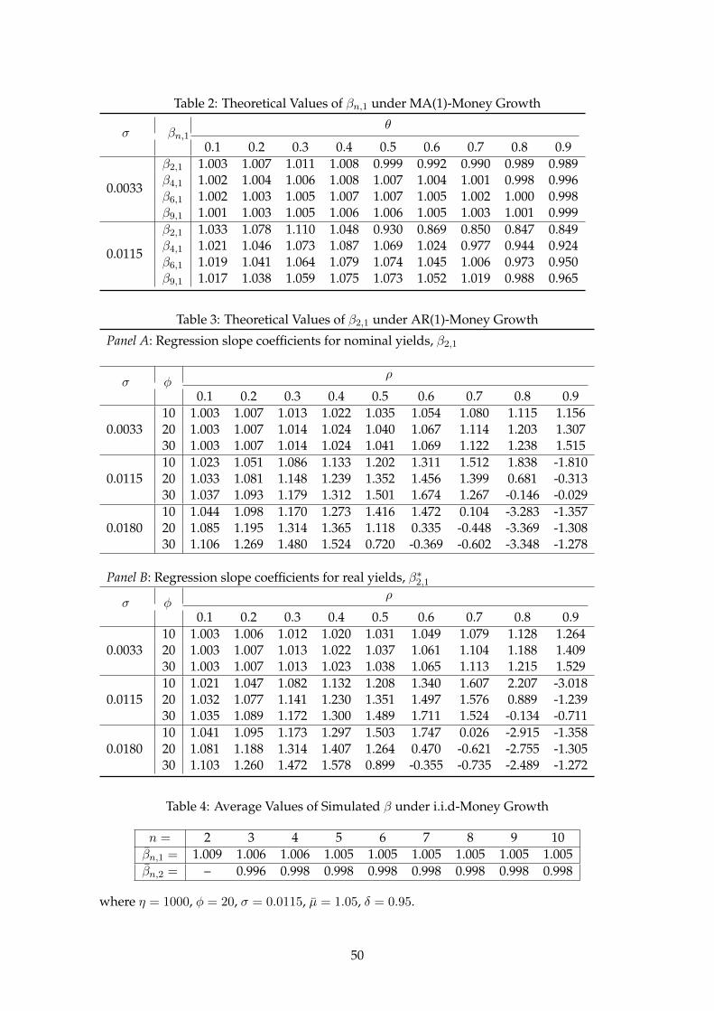
Table 2: Theoretical Values of βn,1 under MA(1)-Money Growth

σ βn,1θ

0.1 0.2 0.3 0.4 0.5 0.6 0.7 0.8 0.9

0.0033

β2,1 1.003 1.007 1.011 1.008 0.999 0.992 0.990 0.989 0.989β4,1 1.002 1.004 1.006 1.008 1.007 1.004 1.001 0.998 0.996β6,1 1.002 1.003 1.005 1.007 1.007 1.005 1.002 1.000 0.998β9,1 1.001 1.003 1.005 1.006 1.006 1.005 1.003 1.001 0.999

0.0115

β2,1 1.033 1.078 1.110 1.048 0.930 0.869 0.850 0.847 0.849β4,1 1.021 1.046 1.073 1.087 1.069 1.024 0.977 0.944 0.924β6,1 1.019 1.041 1.064 1.079 1.074 1.045 1.006 0.973 0.950β9,1 1.017 1.038 1.059 1.075 1.073 1.052 1.019 0.988 0.965

Table 3: Theoretical Values of β2,1 under AR(1)-Money Growth

Panel A: Regression slope coefficients for nominal yields, β2,1

σ φρ

0.1 0.2 0.3 0.4 0.5 0.6 0.7 0.8 0.9

0.003310 1.003 1.007 1.013 1.022 1.035 1.054 1.080 1.115 1.15620 1.003 1.007 1.014 1.024 1.040 1.067 1.114 1.203 1.30730 1.003 1.007 1.014 1.024 1.041 1.069 1.122 1.238 1.515

0.011510 1.023 1.051 1.086 1.133 1.202 1.311 1.512 1.838 -1.81020 1.033 1.081 1.148 1.239 1.352 1.456 1.399 0.681 -0.31330 1.037 1.093 1.179 1.312 1.501 1.674 1.267 -0.146 -0.029

0.018010 1.044 1.098 1.170 1.273 1.416 1.472 0.104 -3.283 -1.35720 1.085 1.195 1.314 1.365 1.118 0.335 -0.448 -3.369 -1.30830 1.106 1.269 1.480 1.524 0.720 -0.369 -0.602 -3.348 -1.278

Panel B: Regression slope coefficients for real yields, β∗2,1

σ φρ

0.1 0.2 0.3 0.4 0.5 0.6 0.7 0.8 0.9

0.003310 1.003 1.006 1.012 1.020 1.031 1.049 1.079 1.128 1.26420 1.003 1.007 1.013 1.022 1.037 1.061 1.104 1.188 1.40930 1.003 1.007 1.013 1.023 1.038 1.065 1.113 1.215 1.529

0.011510 1.021 1.047 1.082 1.132 1.208 1.340 1.607 2.207 -3.01820 1.032 1.077 1.141 1.230 1.351 1.497 1.576 0.889 -1.23930 1.035 1.089 1.172 1.300 1.489 1.711 1.524 -0.134 -0.711

0.018010 1.041 1.095 1.173 1.297 1.503 1.747 0.026 -2.915 -1.35820 1.081 1.188 1.314 1.407 1.264 0.470 -0.621 -2.755 -1.30530 1.103 1.260 1.472 1.578 0.899 -0.355 -0.735 -2.489 -1.272

Table 4: Average Values of Simulated β under i.i.d-Money Growth

n = 2 3 4 5 6 7 8 9 10βn,1 = 1.009 1.006 1.006 1.005 1.005 1.005 1.005 1.005 1.005βn,2 = – 0.996 0.998 0.998 0.998 0.998 0.998 0.998 0.998

where η = 1000, φ = 20, σ = 0.0115, µ = 1.05, δ = 0.95.

50

Table 5: Average Values of Simulated β under MA(1)-Money Growth

n = 2 3 4 5 6 7 8 9 10βn,1 = 0.857 0.897 0.924 0.939 0.949 0.955 0.960 0.963 0.966βn,2 = – 1.037 1.018 1.015 1.014 1.013 1.012 1.012 1.012

where η = 1000, φ = 20, σ = 0.0115, µ = 1.05, δ = 0.95, θ = 0.9.

Table 6: Average Values of Simulated βn,m under AR(1)-Money Growth

Panel A: Regression slope coefficients for nominal yields, βn,m

σ ρ mn

2 3 4 5 6 7 8 9 10

0.0080

0.61 1.458 1.375 1.326 1.294 1.272 1.256 1.244 1.235 1.228

2 – 1.301 1.240 1.204 1.181 1.165 1.154 1.146 1.140

0.91 1.088 1.102 1.123 1.148 1.175 1.204 1.234 1.263 1.292

2 – 1.164 1.174 1.188 1.206 1.226 1.248 1.270 1.293

0.0115

0.61 1.565 1.487 1.439 1.407 1.385 1.369 1.357 1.348 1.340

2 – 1.444 1.369 1.322 1.291 1.270 1.255 1.243 1.234

0.91 0.214 0.160 0.065 -0.036 -0.129 -0.207 -0.266 -0.308 -0.335

2 – 0.471 0.327 0.191 0.067 -0.032 -0.115 -0.178 -0.224

Panel B: Regression slope coefficients for real yields, β∗n,m

σ ρ mn

2 3 4 5 6 7 8 9 10

0.0080

0.61 1.440 1.345 1.326 1.292 1.259 1.238 1.223 1.212 1.204

2 – 1.261 1.203 1.171 1.151 1.138 1.129 1.122 1.117

0.91 1.550 1.690 1.800 1.884 1.948 1.995 2.029 2.053 2.070

2 – 1.817 1.896 1.953 1.993 2.020 2.036 2.046 2.051

0.0115

0.61 1.621 1.531 1.473 1.435 1.409 1.389 1.375 1.363 1.354

2 – 1.449 1.367 1.316 1.283 1.261 1.246 1.234 1.225

0.91 -1.073 -1.095 -1.116 -1.132 -1.140 -1.138 -1.126 -1.103 -1.072

2 – -0.733 -0.787 -0.834 -0.872 -0.898 -0.912 -0.913 -0.903

where η = 1000, φ = 20, µ = 1.05, δ = 0.95.

51

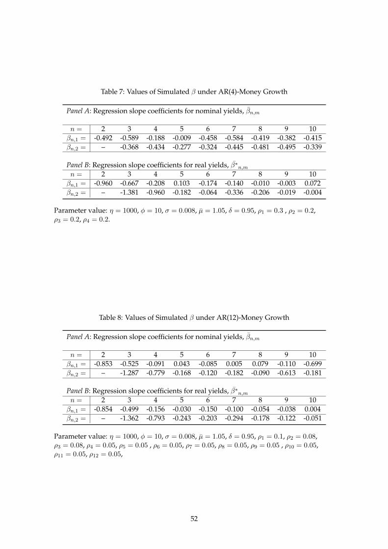
Table 7: Values of Simulated β under AR(4)-Money Growth

Panel A: Regression slope coefficients for nominal yields, βn,m

n = 2 3 4 5 6 7 8 9 10βn,1 = -0.492 -0.589 -0.188 -0.009 -0.458 -0.584 -0.419 -0.382 -0.415βn,2 = – -0.368 -0.434 -0.277 -0.324 -0.445 -0.481 -0.495 -0.339

Panel B: Regression slope coefficients for real yields, β∗n,mn = 2 3 4 5 6 7 8 9 10βn,1 = -0.960 -0.667 -0.208 0.103 -0.174 -0.140 -0.010 -0.003 0.072βn,2 = – -1.381 -0.960 -0.182 -0.064 -0.336 -0.206 -0.019 -0.004

Parameter value: η = 1000, φ = 10, σ = 0.008, µ = 1.05, δ = 0.95, ρ1 = 0.3 , ρ2 = 0.2,ρ3 = 0.2, ρ4 = 0.2.

Table 8: Values of Simulated β under AR(12)-Money Growth

Panel A: Regression slope coefficients for nominal yields, βn,m

n = 2 3 4 5 6 7 8 9 10βn,1 = -0.853 -0.525 -0.091 0.043 -0.085 0.005 0.079 -0.110 -0.699βn,2 = – -1.287 -0.779 -0.168 -0.120 -0.182 -0.090 -0.613 -0.181

Panel B: Regression slope coefficients for real yields, β∗n,mn = 2 3 4 5 6 7 8 9 10βn,1 = -0.854 -0.499 -0.156 -0.030 -0.150 -0.100 -0.054 -0.038 0.004βn,2 = – -1.362 -0.793 -0.243 -0.203 -0.294 -0.178 -0.122 -0.051

Parameter value: η = 1000, φ = 10, σ = 0.008, µ = 1.05, δ = 0.95, ρ1 = 0.1, ρ2 = 0.08,ρ3 = 0.08, ρ4 = 0.05, ρ5 = 0.05 , ρ6 = 0.05, ρ7 = 0.05, ρ8 = 0.05, ρ9 = 0.05 , ρ10 = 0.05,ρ11 = 0.05, ρ12 = 0.05,

52

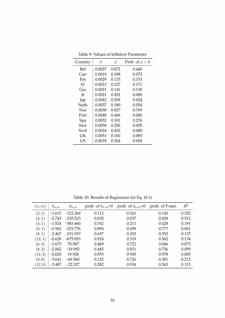
Table 9: Values of Inflation Parameter

Country σ ρ Prob. of ρ = 0

Bel 0.0027 0.072 0.440Can 0.0019 0.188 0.072Fin 0.0029 0.133 0.153Fr 0.0021 0.127 0.171

Ger 0.0031 0.141 0.130It 0.0021 0.452 0.000

Jap 0.0042 0.209 0.024Neth 0.0037 0.180 0.054Nor 0.0030 0.027 0.769Port 0.0048 0.406 0.000Spa 0.0032 0.101 0.276Swe 0.0058 0.256 0.005Swit 0.0024 0.432 0.000UK 0.0051 0.160 0.085US 0.0018 0.264 0.004

Table 10: Results of Regression for Eq. (6.1)

(n,m) bn,m dn,m prob. of bn,m=0 prob. of dn,m=0 prob. of F-stat. R2

(2, 1) -1.615 -122.269 0.112 0.161 0.143 0.322(3, 1) -2.743 -235.523 0.035 0.037 0.028 0.512(4, 1) -1.524 -583.460 0.762 0.211 0.428 0.191(6, 1) -0.562 -253.776 0.894 0.499 0.777 0.061(9, 1) -2.467 -531.937 0.657 0.292 0.553 0.137(12, 1) -0.628 -675.853 0.924 0.319 0.562 0.134(6, 3) -1.675 70.987 0.469 0.722 0.686 0.073(9, 3) -2.062 -19.992 0.445 0.931 0.736 0.059(12, 3) -0.620 19.928 0.853 0.945 0.978 0.005(9, 6) -3.641 -69.560 0.132 0.726 0.301 0.213(12, 6) -3.487 -22.527 0.282 0.934 0.543 0.115

53

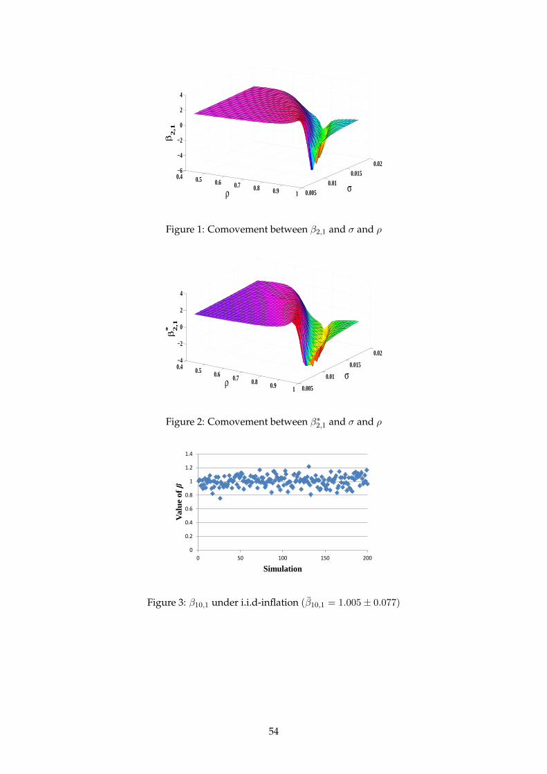
0.4 0.5 0.6 0.7 0.8 0.9 1 0.0050.01

0.0150.02

−6

−4

−2

0

2

4

σρ

β2,1

Figure 1: Comovement between β2,1 and σ and ρ

0.4 0.5 0.6 0.7 0.8 0.9 1 0.005

0.01

0.015

0.02−4

−2

0

2

4

σρ

β2

,1*

Figure 2: Comovement between β∗2,1 and σ and ρ

0

0.2

0.4

0.6

0.8

1

1.2

1.4

0 50 100 150 200

Va

lue o

f β

Simulation

Figure 3: β10,1 under i.i.d-inflation (β10,1 = 1.005± 0.077)

54

0

0.2

0.4

0.6

0.8

1

1.2

1.4

0 50 100 150 200

Va

lue o

f β

Simulation

Figure 4: β10,2 under i.i.d-inflation (β10,2 = 0.998± 0.093)

0

0.2

0.4

0.6

0.8

1

1.2

1.4

0 50 100 150 200

Va

lue o

f β

Simulation

Figure 5: β10,1 under MA(1)-inflation (β10,1 = 0.966± 0.102)

0

0.2

0.4

0.6

0.8

1

1.2

1.4

0 50 100 150 200

Va

lue o

f β

Simulation

Figure 6: β10,2 under MA(1)-inflation (β10,2 = 1.012± 0.103)

55

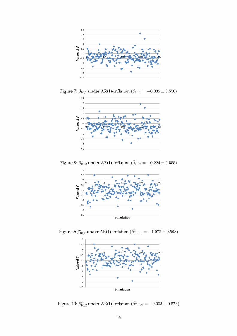
-2.5

-2

-1.5

-1

-0.5

0

0.5

1

1.5

2

2.5

0 50 100 150 200

Valu

es o

f β

Figure 7: β10,1 under AR(1)-inflation (β10,1 = −0.335± 0.550)

-2.5

-2

-1.5

-1

-0.5

0

0.5

1

1.5

2

2.5

0 50 100 150 200

Va

lues

of β

Figure 8: β10,2 under AR(1)-inflation (β10,2 = −0.224± 0.555)

-3.5

-3

-2.5

-2

-1.5

-1

-0.5

0

0.5

1

0 50 100 150 200

Va

lue

of β

Simulation

Figure 9: β∗10,1 under AR(1)-inflation (β∗10,1 = −1.072± 0.598)

-3.5

-3

-2.5

-2

-1.5

-1

-0.5

0

0.5

1

0 50 100 150 200

Va

lue

of β

Simulation

Figure 10: β∗10,2 under AR(1)-inflation (β∗10,2 = −0.903± 0.578)

56

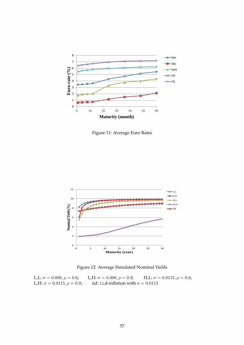
0

1

2

3

4

5

6

7

8

0 10 20 30 40 50 60

Eu

ro-r

ate

(%

)

Maturity (month)

Ger

Jap

Swit

UK

US

Figure 11: Average Euro Rates

0

2

4

6

8

10

12

0 5 10 15 20 25 30

Nom

inal

Yie

ld (

%)

Maturity (year)

L,L

L,H

H,L

H,H

iid

Figure 12: Average Simulated Nominal Yields

L,L: σ = 0.008, ρ = 0.6; L,H: σ = 0.008, ρ = 0.9; H,L: σ = 0.0115, ρ = 0.6;L,H: σ = 0.0115, ρ = 0.9; iid: i.i.d-inflation with σ = 0.0115

57

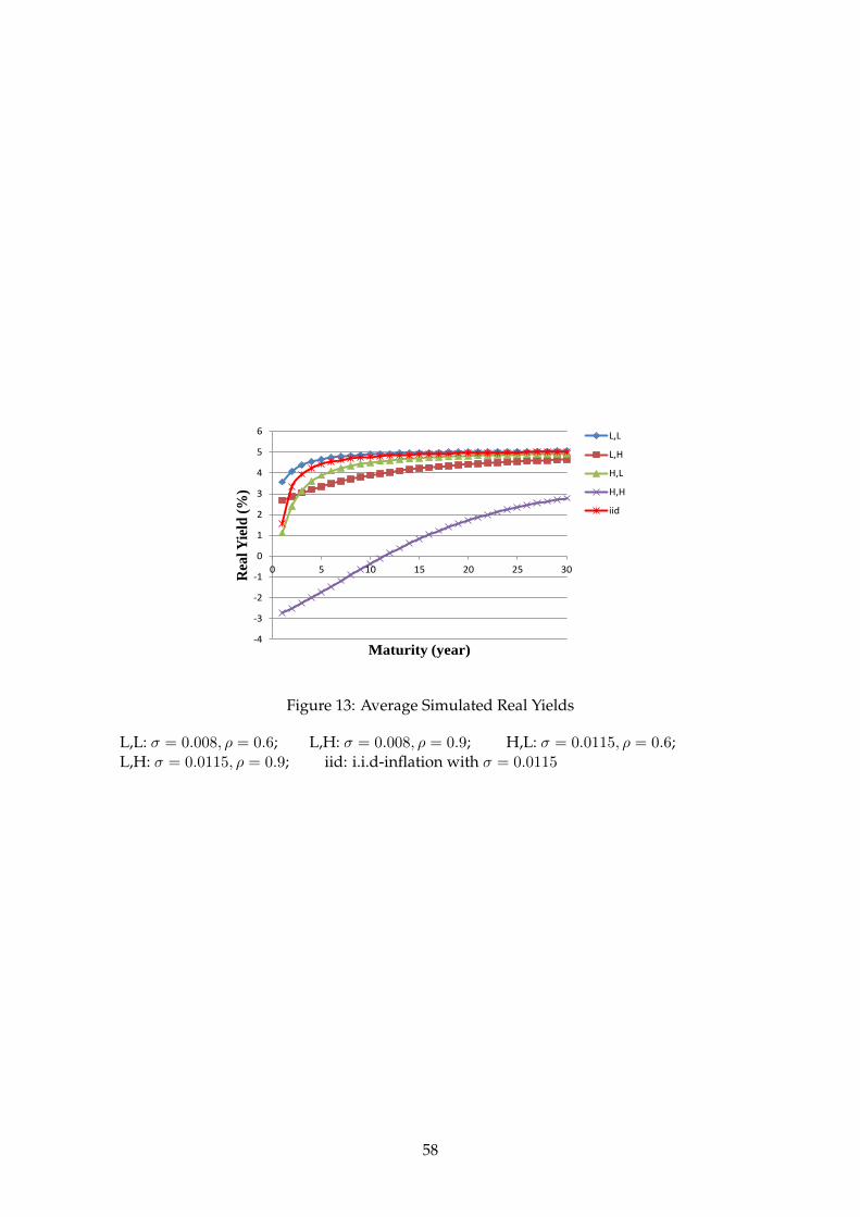
-4

-3

-2

-1

0

1

2

3

4

5

6

0 5 10 15 20 25 30

Rea

l Y

ield

(%

)

Maturity (year)

L,L

L,H

H,L

H,H

iid

Figure 13: Average Simulated Real Yields

L,L: σ = 0.008, ρ = 0.6; L,H: σ = 0.008, ρ = 0.9; H,L: σ = 0.0115, ρ = 0.6;L,H: σ = 0.0115, ρ = 0.9; iid: i.i.d-inflation with σ = 0.0115

58