LLEE Working Paper Series

RESISTING TO THE EXTORTION RACKET: AN EMPIRICAL

ANALYSIS

Michele Battisti Andrea Mario Lavezzi Lucio Masserini Monica Pratesi Working Paper No. 115

December 2014

Luiss Lab of European Economics

Department of Economics and Business

LUISS Guido Carli Viale Romania 32, 00197, Rome -- Italy

http://dptea.luiss.edu/research-centers/luiss-lab-european-economics

© Michele Battisti Andrea Mario Lavezzi Lucio Masserini Monica Pratesi. The aim of

the series is to diffuse the research conducted by Luiss Lab Fellows. The series accepts external contributions whose topics is related to the research fields of the Center. The

views expressed in the articles are those of the authors and cannot be attributed to Luiss

Lab.

Resisting to the Extortion Racket: an Empirical

Analysis

Michele Battisti∗ Andrea Mario Lavezzi † Lucio Masserini‡

Monica Pratesi§

Abstract

In this paper we perform a statistical evaluation of whether it is worthwhile, in

economic terms, to resist to extortion demands by the mafia, from the point of view

of firms operating in an area dominated by criminal organizations. We use a unique

collected and matched database on firm characteristics on the city of Palermo, highly

controlled by the mafia racket. The underlined idea is that the claimed resistance

has (direct and indirect) costs and benefits, so that a rational firm should take

this decision according its economic expectations on the future profits (in addition

to potential ethic considerations). It means that the economic policy messages of

this experience can be linked to make more profitable the racket resistance (as a

signal sent to the market). Our evidences based on multilevel discrete choice models

show that this decision is strongly influenced by socio-economic characteristics of

the district, type of activity involved and other factors.

Keywords Organized Crime, Racketeering, Economic Growth, Discrete choice mod-

els.

JEL classification O17, K42, R11, C41

∗Universita di Palermo†Universita di Palermo‡Universita di Pisa§Universita di Pisa

1

1 Introduction

Extortion is a typical activity performed by criminal organizations such as the Sicilian

Mafia (Gambetta , 1993, Konrad and Skaperdas , 1998, Varese , 2014, Balletta and Lavezzi

, 2014). Extortion consists in the forced extraction of financial resources from firms, under

the threat of punishment for those not complying. Some authors (see in particular Gam-

betta , 1993, Varese , 2014) have highlighted a distinction between the forced extraction

of resources and the genuine payment for services that criminal organization can provide,

as various forms of protection.1

Firms, however, may refuse to pay. This work aims at assessing the determinants

of firms’ behaviour with respect to extortion. In particular, we address the issue of the

determinants of firms’ resistance to extortion, in a context where such behaviour can

be a way to build reputation and attract consumers. Starting from a unique dataset of

firms from the city of Palermo, Sicily, that publicly signalled themselves as non payers

or resistant to the extortion racket, we perform a statistical analysis to investigate the

determinants of the decision to publicly declare to be a resistant. The firms we study

are those that joined Addiopizzo, a Palermo-based NGO that, from 2004, invited firms

declaring refusal to pay the local Mafia to join the NGO and become a member of a public

list, aimed at addressing civic-minded consumers to buy their products or services.2

The steps we followed to construct the dataset are the following: i) we built a sample

of 150 Addiopizzo firms; ii) the list of AP joiners (our study group) has been enriched by

auxiliary information from Census data on Palermo districts. The linkage between the

two sources has been done by a geographical matching by the address of the joiner and the

Enumeration District database; iii) the new AP list has been matched with the CCIAA3

data set of subscribers containing information on balance sheets;4 iv) a stratified random

1Following Varese (2006, p. 412), we can list the following “services”: “protection against extortion...;

protection against theft and police harassment...; protection of thieves...; protection in relation to infor-

mally obtained credit and the retrieval of loans...; elimination of competitors...; intimidation of customers,

workers, and trade unionists for the benefit of employers...; intimidation of lawful right-holders...; and

the settlement of a variety of disputes...”. See Varese (2006, p. 412) for references. In this perspective,

extortion can be defined as: “the forced extraction of resources for services that are promised by not

provided” (Varese , 2014, p. 344).2Consumers wishing to signal their choice to support the Addiopizzo stores, may join a specific list,

which is also publicly available.3CCIAA is the acronym of the Italian Chamber of Commerce network. We extracted the data from

the databank of CERVED, a private company that collects and organizes data from the CCIAA system.4In Italy every legal firm must have a CCIAA position, and every joint stock company must deposit

its balance sheets to the local CCIAA.

2

sample of active firms has been selected from the CCIAA positions of not AP-joiners

(control group). The stratification criteria (see section 3 for details) balanced the control

group by firm’s age.

Our main results are:

1. Notwithstanding a quite similar production function estimation, the probability to

be a joiner is more associated with younger and big (in terms of labour intensive

factor) firms.

2. The stock of assets is negatively associated to the probability to join (as a measure

of risk).

3. Finally, there is an effect related to the firm location, where we have a positive

variance associated with the district level, partly explained by population and partly

by human capital endowment (more educated district have higher joining rates).

The paper is organized as follows: in Section 2 we summarize the history of Addiopizzo

together with a review of the relevant literature; in Section 3 we describe the dataset; Sec-

tion 4 contains the empirical analysis: in particular Section 4.1 provides the descriptive

statistics while Section 4.2 contains the econometric analysis; Section 5 contains conclud-

ing remarks and directions for further research.

2 The Addiopizzo experience and related literature

Addiopizzo (AP henceforth) means “farewell to pizzo”, where pizzo is the Sicilian defi-

nition of the money extorted by the local Mafia, Cosa Nostra.5 AP activity begun from

an idea of few young activists who, in the night of June 29th, 2004, flooded the walls of

Palermo with thousands of stickers carrying the slogan: “A whole people who pays the

pizzo is a people without dignity”. This was a shocking message in a city where it is

estimated that more than 80% of firms and stores pay the extortion racket (Confesercenti

, 2010).

In 2005 the founders of AP organized a campaign to spread this message of resistance

to the racket. In May 2006 a list of more than 100 businesses available to publicly

denounce the pizzo, claiming their refusal to pay, was published in a local newspaper and

diffusion on national media followed. In the years after 2004, more than 1000 firms have

5Thorough accounts of the Sicilian mafia are given, among others, by Gambetta (1993) and Paoli

(2003).

3

been members of AP and at the time we collected the data (May 2012), the number of

joiners was around 820. The list is publicly available.6 Occasionally, AP runs campaigns

targeted to firms of specific neighborhoods of Palermo, organizes meetings in schools, and

holds a regular event in May, “Fiera del consumo critico”, in which AP firms present their

products and various actitivities, from debates to live performances, take place.7

The idea of making public the list of joiners follows an economic insight. Consumers,

in fact, are invited to shop at the AP stores if they wish to: “pay those who do not pay”.8

In other words, AP tries to elicit “critical consumption” by civic-minded citizens. AP

stores clearly signal their membership by displaying an AP sticker at the entrance of their

premises.

In this paper we try to answer the following question: why some firms join AP?9 From

the previous discussion, we can highlight two crucial aspects. The first one regards the

characteristics of the firms and the expectation they have of the consequences of joining

AP.10 Which firms, therefore, are more likely to join? Does, for example, their size or

their sector matter? As long as joining AP exposes firms to risks, then the amount of

capital invested may influence the decision. The sector where the firm operates may play

a role for example because some sectors are more heavily controlled by the Mafia, like

Construction, or because the sector is a proxy for unobservable characteristics of firms’

owners, which may be more or less inclined to resist to the Mafia. Firms’ characteristics

will be the first-level variables considered in the econometric analysis.

The second aspect regards the environment where the firm operates. In particular,

the spread of anti-mafia values in the population is important, as purchases in AP stores

can be considered as an anti-mafia act, under the assumption that shopping in non-AP

stores would feed the Mafia through extorted resources. In this paper we control for

the socio-economic characteristics of the geographical environment of the firm, i..e of the

district where it is located, as second-level variables in the econometric analysis.

6See http://www.addiopizzo.org. A firm may leave the AP list for various reasons: going out of

business, changes in ownership, with new owners asking to be cancelled, cancellation if interactions with

organized crime are detected (see below).7AP also supplies legal support in trials against the racketeers, mainly through the linked business

association Libero Futuro, or psychological support to entrepreneurs considering to refuse to pay the Mafia.

For more details, see Forno and Gunnarson (2010, pp. 109-111) and Gunnarsson (2014, pp.42-44).8This is another slogan diffused by AP.9This question echoes the question raised by Schelling (1971): why some firms’ are victims of extor-

tion? See Lavezzi (2008) for an empirical assessment.10In a companion paper (Battisti et al. , 2014) we analyze the consequences for the economic perfor-

mance for a firm joining AP.

4

Our paper is related to various strands of literature. First of all, to the literature on

extortion implemented by organized crime. For example, Konrad and Skaperdas (1998)

and Bueno de Mesquita and Hafer (2007) present theoretical models of extortion, Varese

(2014) critically analyzes the distinction between extortion and protection, Asmundo and

Lisciandra (2008) offer an empriical evaluation of the impact of extortion on regional GDP

in Sicily, while Alexander (1997) and Balletta and Lavezzi (2014) combine a theoretical

analyis with an emprirical analysis of extortion at firm level.11 None of these articles,

however, deal with the decision of the firms to resist the extortion racket.

Our work is also related to the literature on anti-mafia mobilization by the civil so-

ciety. For example, Akerlof and Yellen (1994) focus on the “community” values that

may influence the behaviour of citizens with respect to criminal gangs and the State;12

Schneider and Schneider (2003) thoroughly analyze the case of Palermo, and reconstruct

the history of the local antimafia movement and its evolution from the peasant move-

ments of the fifties to the more recent, urban-based movements that developed in the

eighties and the nineties, in particular after tragic events like the murders of journalist

Giuseppe Impastato in 1978, Prefect Dalla Chiesa in 1982 or judges Falcone and Borsellino

in 1992.13 The recent experience of AP is read under a historical perspective by Forno

and Gunnarson (2010) who note that, interestingly, AP did not follow sensational events

like violent murders of key persons.14 Finally, La Spina (2008) and Lavezzi (2014) read

the AP experience in the perspective of a more general discussion of the possible anti-

mafia strategies. All of these studies are, however, purely descriptive and, even if they

are oriented to explain the anti-mafia behaviour, they do not offer an answer to the two

above mentioned questions. In this work we propose a statistical model to estimate the

probability of joining AP and to give evidence to answer to these questions.

Finally, our work is related to other scholarly works that specifically focus on AP.

Partridge (2012) studied the choice to become “critical consumers” by a survey. The

consumers surveyed are those that joined an AP consumers’ list which can be consulted

in the AP webpage. He finds that the respondents to the survey are in a high proportion

in the age bracket 30-39, are likely to have a degree and to live in some of the central

11See also Lotspeich (1997) and Varese (2001) on extortion by the Russian Mafia.12A similar point is made by Ramella and Trigilia (1997, p. 25)13Jamieson (2000) analyzes in a broader perspective the antimafia reactions to the murders of 1992,

also discussing the role of Italian politics, police forces and international actors.14An early call for boycotting “Mafia business” was launched by the “Sheets committee”, a movement

mostly led by women, who appeared after assassination of judge Falcone, among the list of guidelines for

citizens wishing to contrast the Mafia. The businesses mentioned were, however, those related to illegal

trades like drugs and cigarettes. See Jamieson (2000, p. 131).

5

Palermo districts.15 In addition, Partridge (2012) finds that the main determinants of

the choice to be “critical consumers” are the willingness to support an organization led

by young people, and to fight the Mafia by “everyday shoppping” (Forno and Gunnarson

, 2010). The main limitation of this analysis is that, as the author recognizes, the lack of

control for the self-selection of the respondents to the survey (and, we may add, for the

self-selection of members of the sampled population to join the public AP list). Forno

and Gunnarson (2010), instead, discuss the AP experience in the more general context

of social mobilization and other form of critical consumption.

Some papers specifically focus on firms’ choice to join AP. Vaccaro (2012) and Vaccaro

and Palazzo (2014), adopting the perspective of business management, indirectly analyze

such firms’ decisions. Specifically, they study the behaviour of AP and how it contributed

to the activation of the firms. They show that AP has been able to attract firms by

strengthen its crediibility as an organization, in particular through the strategic disclosure

of information about its own activities (e.g. on its budget) and on external activities (e.g.

of Mafia), while Vaccaro and Palazzo (2014) emphasize the strategic use of values to

elicit activation of firms and other agents such as consumers, students and members of

the society at large.

Gunnarsson (2014), as we do in this paper, directly focuses on firms’ decision to join

AP. The sample and the methodology are, however, very different from ours: the sample

is represented by the respondents to a survey, and does not include a control group and

second-level variables. The variables considered in the research are also different from

ours. In particular, Gunnarsson (2014) aims at assessing the role played by networks and

trust. The networks analyzed are those involving AP firms but created by membership

to associations different from AP (e.g. environmental, political, economic), or by family

and other personal ties. Variables extracted from the survey are then used as regressors

to explain the different timing of joining AP. Results show that early joiners are different

from late joiners: their decision being based more strongly on membership to ”action

groups” and on family ties. Trust is instead found important for the decision of joiners

that were not contacted by any member of their networks.

Finally, the recent paper by La Rosa et al. (2013) aims at studying the determinants

of firms’ decision to join AP adopting, as we do, a logistic regression approach. The

main findings are that the leverage of firms and firms’ size have a negative impact on the

probability to join. Their sample is, however, very different: it is a self selected sample,

15These districts are Politeama, Liberta’ and Resuttana-San Lorenzo. See Section 4.1 for a discussion

of Palermo districts.

6

as ours, but it is not accompanied by a random control group. Our matching procedure

allow us to have auxiliary variables at firm level (first level variables) and at district level

(second level auxiliary variables). This provides us the information to separate the effect

of individual factors from that of, say, environmental factors on the probability of joining

AP.16

A caveat of the analysis of AP firms is that, even if with a very high probability

they do not pay the pizzo, we are not able to control for the firms’ truthful disclosure

of information.17 As discussed by Vaccaro (2012, p. 7), firms can be ”double-game”

players and choose to join an anti-racket organization to mask their actual connections

with organized crime.18 On the one hand, AP closely monitors the firms and has already

expelled some ”double-game” players.19. On the other hand, this is not relevant for

this study because the observable declaration is anyway seen as a signal on the market,

which may have positive consumption effects due to reputation (as a sort of customer

discrimination in Becker , 1957), while acquiescence may avoid problems due to higher

risks, that may be reflected for instance in indirect costs, such as higher interest rates, and

direct costs, such as damages inflicted by the criminal organization. In other words we

are forced to study the probability of declaring to have joined AP. This can be different

from the probability of actual not payment of the Pizzo.

3 The Data

The dataset we built consists of two types of data: first-level data, i.e. firm-specific data

and second-level data, i.e. data on the district where the firms are located. We have two

groups of firms: firms that joined AP, and a control group of non-joiners. We only consider

limited-liability firms, because they are the only type who must make their balance sheets

public, by handing them in the Chambers of Commerce.

We obtained information on AP firms directly from Addiopizzo: this include qualitative

information such as the sector, the location, and the date of joining AP.20 We added

16La Rosa et al. (2013) also analyze the consequences on firms’ economic performance of joining AP by

comparing mean values of selected variables across the two groups or within the group of AP firms before

and after joining. In Battisti et al. (2014) we study this issue with our sample, adopting a diff-in-diff

strategy.17When joining AP, firms must sign a declaration of non compliance with extortionary requests.18Indeed, some evidence shows that mafia bosses may suggest to strategically join anti-mafia organi-

zations for this purpose. See Vaccaro (2012, p. 7).19Personal communication confirmed this.20The date in which a firm joined AP is the only one not publicly available.

7

quantitative data from balance sheets of these firms from the CERVED dataset. The

data on the districts are from the 2001 Census and, therefore, reflect the socio-economic

conditions prior the creation of AP and should be exogenous with respect to the choice

of joining AP.

The original dataset on AP firms has 839 entries, and refers to firms that joined within

May 2012. The same firms may appear more than one if they have more branches. From

the initial 839 entries we eliminate entries referred to firms outside of the province of

Palermo (69) and entries related to branches.

The proportion among group 1. and 2. is given that 2. is three times bigger than 1. In

order to build a database with the characteristics we needed to implement the econometric

analysis relative to firms’ choices in order to declare/not declare racket resistance we used:

• Information on joiners. Year, location, sector, address for 839 firms, 72% of whom

within the municipality of Palermo. We got this information from AP: while the

list of firms is public, the membership date had been kindly supplied from them.

• Census and geo-spatial data at sub-block level for the city of Palermo (3021 census

cells and 25 districts) supplied from National Statistic Institure ISTAT for the census

200121.

• Budget data from CCIAA for the years 2002-2011 (244 joiners and a control group of

non-joiners of 732 randomly selected firms) as revenues, costs, cash, bank debts, data

on employees and labour costs, assets, net patrimony and depreciation rates. For

non limited liability firms (for those is not compulsory the delivery of budget data)

we have just some basic information as number of employees and legal minimum

requirement of patrimony to start the activity. These data are hystorically used to

be delivered in paper form in Italy to the Chamber of Commerce System that is

part of Statistical National System (SISTAN). Finally we bought these data from

Cerved that is a private firm that collects and puts in electronic format.

• Toponomymic data in order to match data at point 2 to data at points 1, 3. These

were supplied from the Municipality of Palermo, Department of Topography.

We started from the AP joiners group and with the addressess we match them to the

census and district data through toponomymic information. Then we did the same for

21The census data are collected every 10 years. We decided to choose 2001 over 2011 in order to have

choices of the firms based on territory characteristics already known when they decide to choose, in order

to avoid simultaneity/endogeneity issues, given AP starts in 2005 and our sample is collected until 2012.

8

the random sample group. At the end we have firm data and district characteristics for

joiners and non joiners.

At the time we collected this database it had 839 entries (actually, at the beginning

of 2014 is 820 due to the natural turnover of new firms entered, old firms out of activity

and so on). From the initial 839 entries we eliminate firms out of the province of Palermo

(69) and collapse firms with local units that have repeated values for budget data. The

joiners group is composed of 244 limited liability firms (190 within the municipality),

close to 5% of the total number of firms for the city. Then with a small amount of

information (number of workers, firm age, location) we have other 192 firms (individual

and associations) from the province of Palermo and other 9 firms (the legal nature being

uncertain). The control group has a proportion 3:1, so there are 732 limited liability and

576 other firms randomly selected.

Then we have some data for the remaining 112 firms of Palermo province without

an identification number. It means that our working sample has 732+244=976 firms for

whom we have all data sources. The budget data are, by construction, nominal data so we

weight with the PCI of Palermo city, supplied from ISTAT, in order to make the variables

in real terms. To summarize for every firm we will use in our econometric specification:

• firm budget real variables: revenues, costs, assets, employees, value added, cash,

bank debt, depreciation.

• census/district variables: education, labour market, demography

Finally we averaged over the budget year available for every firm in order to avoid

ciclicality and we end with a cross sectional database of 576 useful limited liability obser-

vations.

4 Empirical Analysis

4.1 Descriptive statistics

In this section we provide some descriptive statistics of the firms in our sample, in par-

ticular comparing the characteristics of the AP firms to those of the control sample, and

of the territory of the city of Palermo, divided in 25 districts (“Quartieri”).

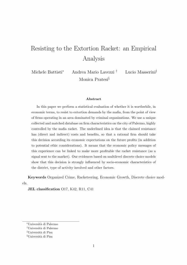
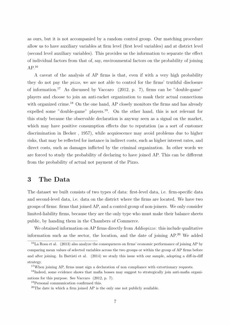
Table 4.1 contains the evolution of the number of joiners in time.

9

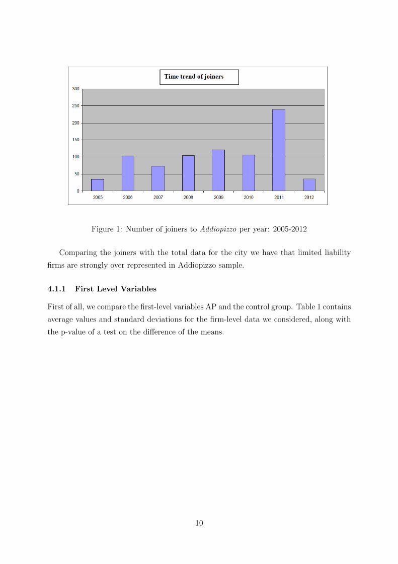
Figure 1: Number of joiners to Addiopizzo per year: 2005-2012

Comparing the joiners with the total data for the city we have that limited liability

firms are strongly over represented in Addiopizzo sample.

4.1.1 First Level Variables

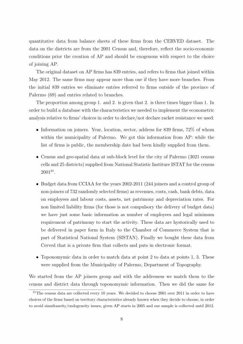
First of all, we compare the first-level variables AP and the control group. Table 1 contains

average values and standard deviations for the firm-level data we considered, along with

the p-value of a test on the difference of the means.

10

AP Control

mean std.dev mean std.dev pval toAv

Assets 748178.32 4709943.16 615897.62 3380364.93 0.75

Cash 104130.05 480005.19 54933.47 175900.32 0.22

Net Partimony 374634.80 1707861.42 251391.39 1271324.14 0.42

Profits -2812.01 81004.82 -20138.31 232021.24 0.16

Debts 463637.72 2652589.76 428064.21 2149966.68 0.88

Revenues 1477937.55 5086066.25 909457.68 3643809.14 0.21

Personnel costs 346859.69 1549325.66 122998.12 404548.88 0.08

Returns -27680.13 112590.88 -22013.90 116237.65 0.59

Gross Profits 41947.74 178315.01 9915.70 169033.71 0.05

Employers (classes) 1.53 0.89 0.85 0.86 0.00

Age of firm 11.90 12.60 15.00 11.22 0.01

Table 1: Distribution across districts (SAMPLE A), non standardized data

Table 1 shows that AP firms have significantly higher levels of personnel costs, gross

profits, number of workers, and a significantly lower firms’ age. However, although the

differences are not significant, AP firms seem to have higher levels of liquidity, of net

wealth, of net profits, of revenues. In other words, they broadly appear are ”healthier”

firms.

Table 2 contains the distribution across sectors.22

num. firms num. firms perc. perc.

Rental and Other Services 10 38 6.67 7.92

Education and Health 7 36 4.67 7.50

Arts, Sports, Entertainments 10 7 6.67 1.46

Manufacturing 13 42 8.67 8.75

Building 13 82 8.67 17.08

Trade and Repairing cars 53 115 35.33 23.96

Transport and Storage 7 19 4.67 3.96

Hotels and Restaurants 12 21 8.00 4.38

High Skill Services 23 78 15.33 16.25

Real Estate 2 42 1.33 8.75

Table 2: Distribution across sectors, Ateco0b (< 1-digit), (SAMPLE A)

22The classification we consider in this paper is based on 10 sectors and is obtained by aggregating the

21 1-digit sectors represented in our sample. Table ??? contains the details of the classification.

11

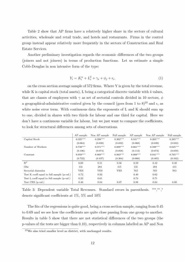
Table 2 show that AP firms have a relatively higher share in the sectors of cultural

activities, wholesale and retail trade, and hotels and restaurants. Firms in the control

group instead appear relatively more frequently in the sectors of Construction and Real

Estate Services.

Another preliminary investigation regards the economic differences of the two groups

(joiners and not joiners) in terms of production functions. Let us estimate a simple

Cobb-Douglas in non intensive form of the type:

Yi = Kαi + Lδi + γs + φj + εi. (1)

on the cross section average sample of 572 firms. Where Y is given by the total revenue,

while K is capital stock (total assets), L being a categorical discrete variable with 4 values,

that are classes of employees with γ as set of sectorial controls divided in 10 sectors, φ

a geographical-administrative control given by the council (goes from 1 to 8)23 and εi as

white noise error term. With continuous data the exponents of L and K should sum up

to one, divided in shares with two thirds for labour and one third for capital. Here we

don’t have a continuous variable for labour, but we just want to compare the coefficients,

to look for structural differences among sets of observations.

AP sample Non AP sample Full sample AP sample Non AP sample Full sample

Capital Stock 0.325∗∗∗ 0.298∗∗∗ 0.302∗∗∗ 0.341∗∗∗ 0.265∗∗∗ 0.285∗∗∗

(0.064) (0.038) (0.032) (0.068) (0.039) (0.033)

Number of Workers 0.739∗∗∗ 0.571∗∗∗ 0.609∗∗∗ 0.661∗∗∗ 0.598∗∗∗ 0.625∗∗∗

(0.106) (0.074) (0.058) (0.112) (0.073) (0.059)

Constant 8.959∗∗∗ 8.869∗∗∗ 8.863∗∗∗ 8.008∗∗∗ 9.041∗∗∗ 8.765∗∗∗

(0.722) (0.437) (0.364) (0.666) (0.405) (0.342)

R2 0.69 0.51 0.56 0.59 0.42 0.48

Obs 131 284 415 131 284 415

Sectorial dummies YES YES YES NO NO NO

Test K coeff equal to full sample (p-val.) 0.72 0.92 0.40 0.62

Test L coeff equal to full sample (p-val.) 0.22 0.61 0.74 0.71

Test CRS (p-val.) 0.46 0.04 0.07 0.98 0.04 0.08

Table 3: Dependent variable Total Revenues. Standard errors in parenthesis. ∗∗∗,∗∗ ,∗

denote significant coefficients at 1%, 5% and 10%

The fits of the regressions is quite good, being a cross section sample, ranging from 0.45

to 0.69 and we see how the coefficients are quite close passing from one group to another.

Results in table 5 show that there are not statistical differences of the two groups (the

p-values of the tests are bigger than 0.10), respectively in columns labelled as AP and Non

23We also tried smaller level as district, with unchanged results.

12

AP with respect of the full sample in column 3 and that the exponent of capital is close

to the textbook level one expects. It means we are not comparing different samples with

respect to the fundamentals of productivity returns, in the view of a production function.

4.1.2 Second Level Variables

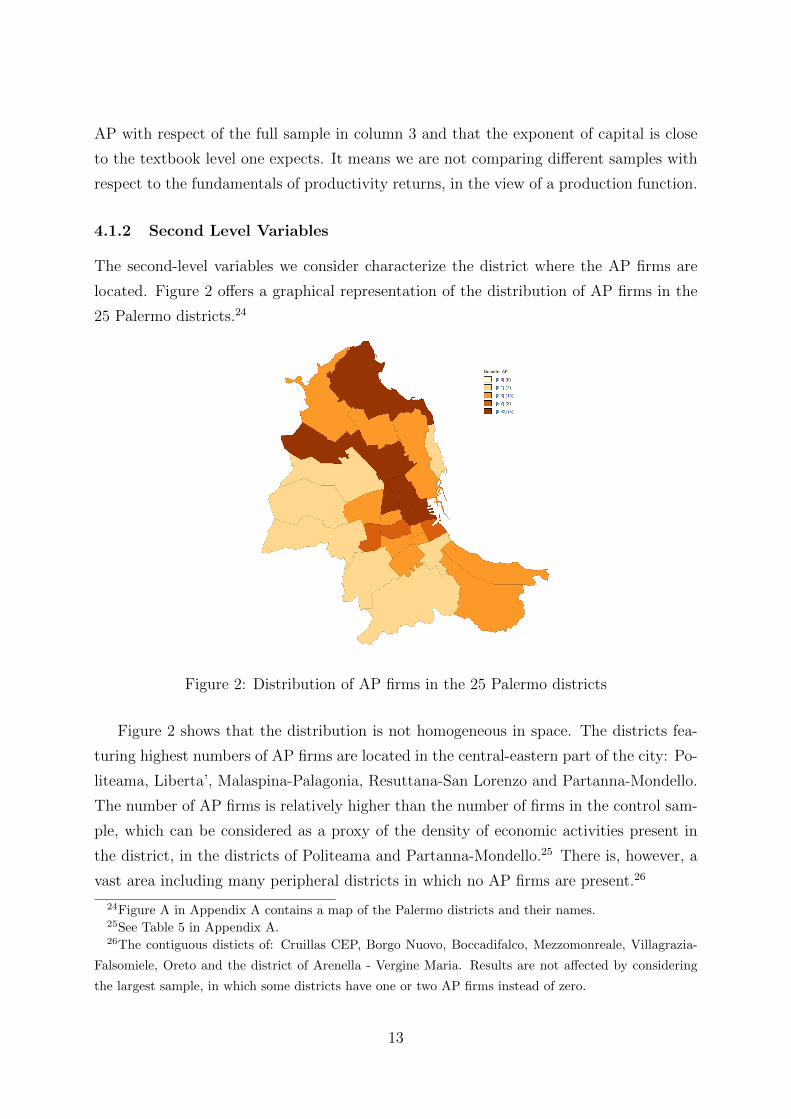
The second-level variables we consider characterize the district where the AP firms are

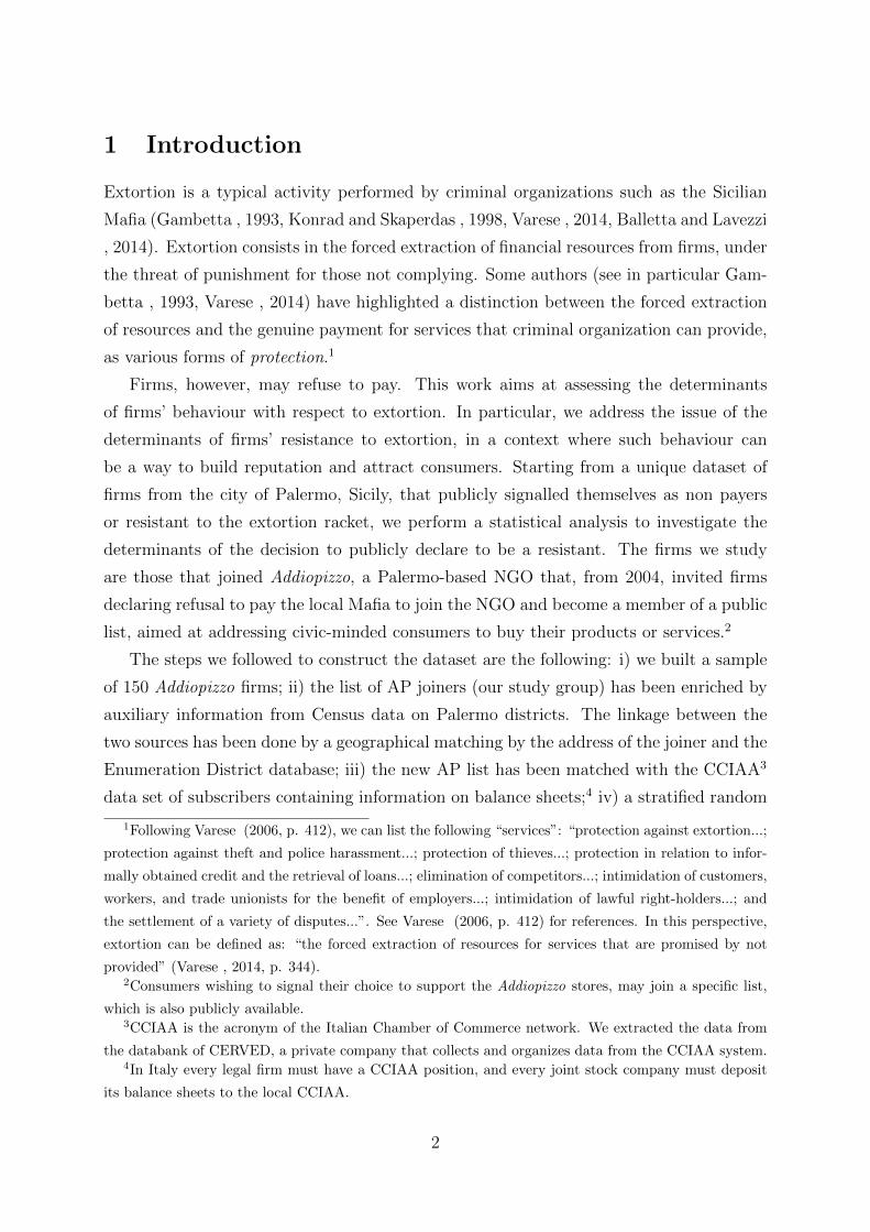
located. Figure 2 offers a graphical representation of the distribution of AP firms in the

25 Palermo districts.24

Figure 2: Distribution of AP firms in the 25 Palermo districts

Figure 2 shows that the distribution is not homogeneous in space. The districts fea-

turing highest numbers of AP firms are located in the central-eastern part of the city: Po-

liteama, Liberta’, Malaspina-Palagonia, Resuttana-San Lorenzo and Partanna-Mondello.

The number of AP firms is relatively higher than the number of firms in the control sam-

ple, which can be considered as a proxy of the density of economic activities present in

the district, in the districts of Politeama and Partanna-Mondello.25 There is, however, a

vast area including many peripheral districts in which no AP firms are present.26

24Figure A in Appendix A contains a map of the Palermo districts and their names.25See Table 5 in Appendix A.26The contiguous disticts of: Cruillas CEP, Borgo Nuovo, Boccadifalco, Mezzomonreale, Villagrazia-

Falsomiele, Oreto and the district of Arenella - Vergine Maria. Results are not affected by considering

the largest sample, in which some districts have one or two AP firms instead of zero.

13

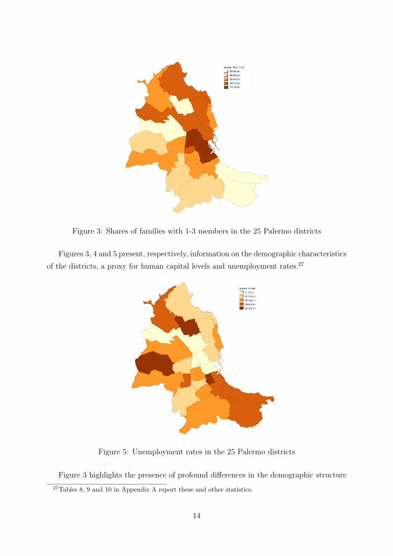
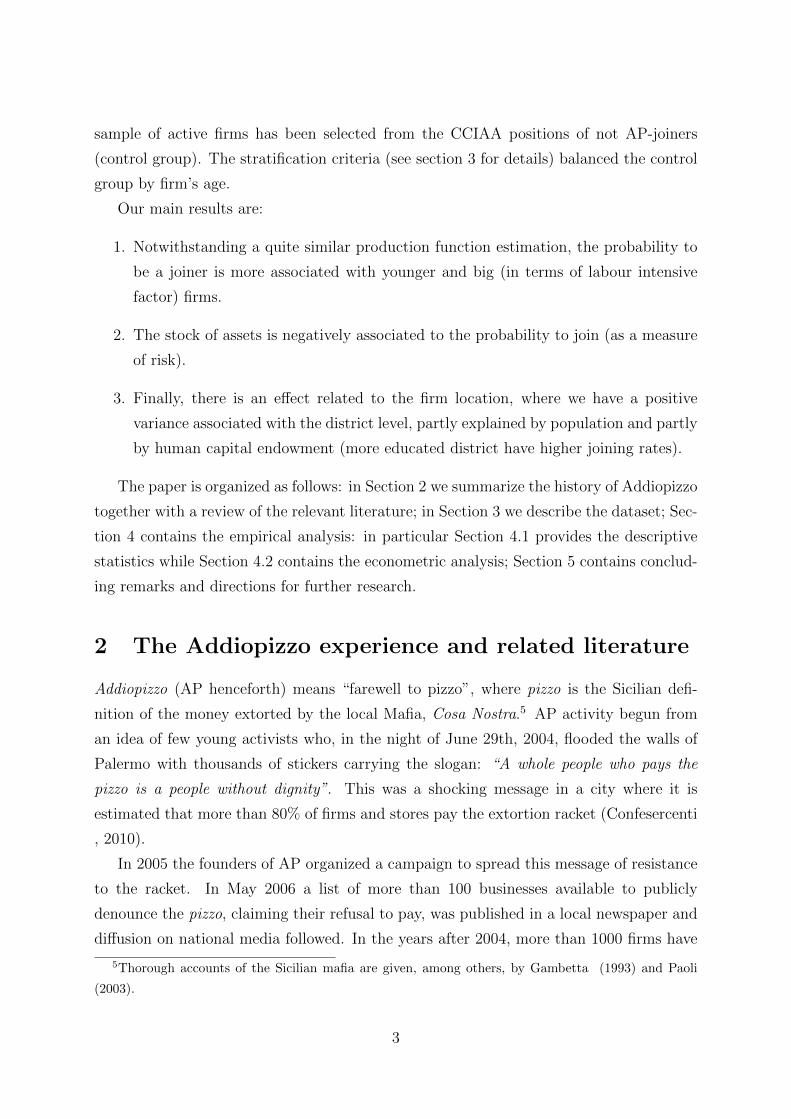
Figure 3: Shares of families with 1-3 members in the 25 Palermo districts

Figures 3, 4 and 5 present, respectively, information on the demographic characteristics

of the districts, a proxy for human capital levels and unemployment rates.27

Figure 5: Unemployment rates in the 25 Palermo districts

Figure 3 highlights the presence of profound differences in the demographic structure

27Tables 8, 9 and 10 in Appendix A report these and other statistics.

14

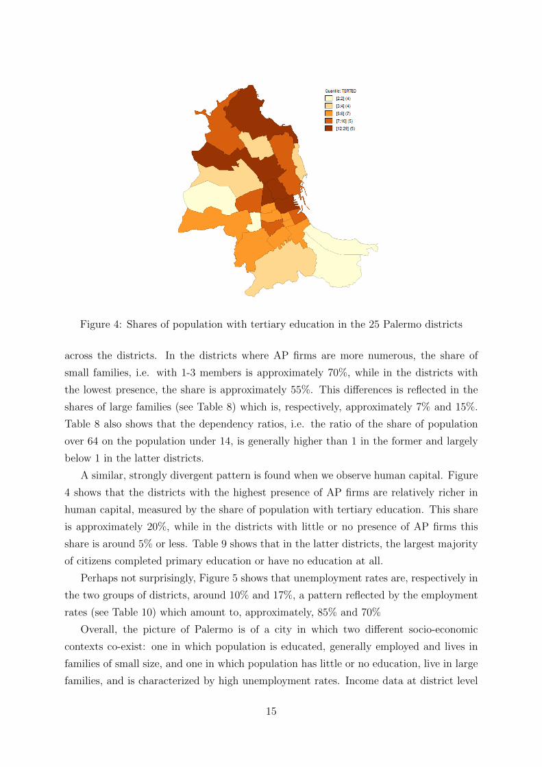
Figure 4: Shares of population with tertiary education in the 25 Palermo districts

across the districts. In the districts where AP firms are more numerous, the share of

small families, i.e. with 1-3 members is approximately 70%, while in the districts with

the lowest presence, the share is approximately 55%. This differences is reflected in the

shares of large families (see Table 8) which is, respectively, approximately 7% and 15%.

Table 8 also shows that the dependency ratios, i.e. the ratio of the share of population

over 64 on the population under 14, is generally higher than 1 in the former and largely

below 1 in the latter districts.

A similar, strongly divergent pattern is found when we observe human capital. Figure

4 shows that the districts with the highest presence of AP firms are relatively richer in

human capital, measured by the share of population with tertiary education. This share

is approximately 20%, while in the districts with little or no presence of AP firms this

share is around 5% or less. Table 9 shows that in the latter districts, the largest majority

of citizens completed primary education or have no education at all.

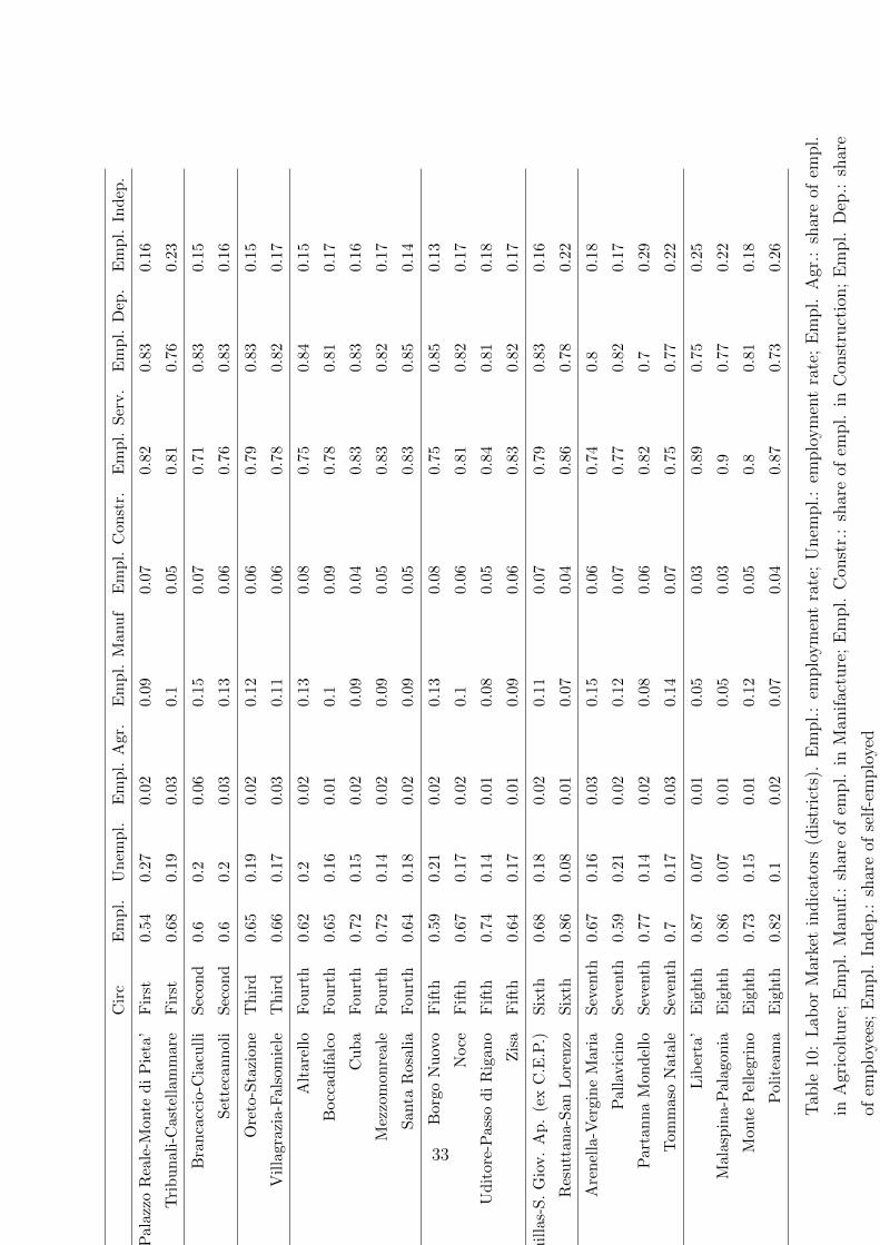
Perhaps not surprisingly, Figure 5 shows that unemployment rates are, respectively in

the two groups of districts, around 10% and 17%, a pattern reflected by the employment

rates (see Table 10) which amount to, approximately, 85% and 70%

Overall, the picture of Palermo is of a city in which two different socio-economic

contexts co-exist: one in which population is educated, generally employed and lives in

families of small size, and one in which population has little or no education, live in large

families, and is characterized by high unemployment rates. Income data at district level

15

are not available, but this picture suggests the coexistence in Palermo of rich and poor

neigbhoroods, where the income differences are likely to be sizeable.

4.2 Econometric analysis

4.2.1 Methodology

Hierarchical or multilevel data are common in the social and behavioral sciences. In

this paper, analysed data show a typical hierarchical structure (Bryk and Raudenbush,

2002; Snijders and Bosker, 2011) where lower-level units (individuals) are nested within

higher-level units (clusters). Here, firms are clustered in neighborhoods and define a

two-level hierarchical data structure. Because of this we can expect that firms located

within each neighborhood, sharing the same unobserved factors, due to the exposure

to common environmental or contextual effects, have correlated values of the response

variable. When this occurs, analyzing lower-level units as if they were independent can

produce biased standard errors of the regression coefficients, thus resulting in erroneous

inferences (Hox, 2010) and possible substantive mistakes when interpreting the effects of

predictor variables. Furthermore, in the analysis of such data, it is usually informative to

take into account the sources of variability in the responses associated with each level of

nesting, in this case the variance between firms and between neighborhoods, respectively.

Multilevel regression models (Goldstein, 2011; Raudenbush and Bryk, 2002; Sneijder

and Bosker, 2011) are suitable for handling dependence among the responses resulting

from a hierarchical data structure, also analysing the complex pattern of variability. In

multilevel models, the total variance of the response variable is partitioned into its different

components of variation, due to the various cluster levels in the data. The effect of

clustering is modelled by introducing random effects (Laird and Ware, 1982), that is a

continuous latent variable following a known parametric distribution, whose values are

constant within clusters but vary across clusters. Independence across observations is

assumed at cluster-level (neighborhood) whereas at individual-level (firms) it is assumed

only among units belonging to different clusters (independence conditional on cluster

membership). As a consequence, cluster-level random effects can be interpreted as the

effects of neighborhood-levels unmeasured covariates that induce dependence among firms

in the same neighborhood whereas indivudual-level random effects represent residuals

specific to each firm after taking into account cluster effects. To explain at least some of

the cluster-level variability, neighborhood-level covariates can also be introduced.

In the literature, multilevel regression models has become known under a variety of

16

names, such as random coefficient model (de Leeuw and Kreft, 1986; Longford, 1987),

variance component model (Longford, 1987), hierarchical linear model (Raudenbush and

Bryk, 1986; 1988) and mixed models (McCulloch, Searle and Neuhaus, 2008). Although

these models are not strictly the same, they can be referred collectively as ”multilevel

regression models” (Hox. 2010). Substantive literature treating multilevel models includes

Bryk and Raudenbush (2002), Gelman and Hill (2007), Snijders and Bosker (2011) and

Hox (2010) for excellent introduction and Longford (1993), Demidenko (2004), de Leeuw

and Meijer (2008a) and Goldstein (2011) for more detailed mathematical background.

In this research, the response variable, indicated with y, is binary and distinguishes

the firms that decided to associate with ”Addiopizzo” by May, 2012 (y = 1) from the

others (y = 0). The analysis is performed by using a two-level random intercepts logistic

regression model (Goldstein, 2011; Rabe-Hesketh, Skrondal and Pickles, 2004). Given a

binary outcome yij [0,1] observed on firm i, with i=1,2,..., Nj, located in neighborhood j,

with j=1,2,..., G and being Pij = Pr(yij = 1) the probability that yij takes on the value

of 1 (a firm associated with ”Addiopizzo”), the model is defined in terms of the natural

logarithm of the odds ratio (logit), indicated as ln(Pij/1 − Pij). Hence, the two-level

random intercepts logistic regression model can be expressed as a linear function of the

explanatory variables using the single equation mixed model formulation (Rabe-Hesketh,

Skrondal and Pickles, 2004):

ln

(Pij

1− Pij

)= β0 + β1xij + γwij + ui (2)

where xij is a vector of predictors for firm i placed in neighborhood j and wj is a vector

of predictors characterizing the neighborhood j. The random effects are given by the level

2 residual, uj N(0, u), which define the effect of being in neighborhood j on the log-odds.

This parameter represent a continuous and unobservable quantity shared by the firms

within a particular neighborhood that captures all the relevant factors not accounted for

by the observed covariates. The magnitude of the standard deviation, u, indicates the

strength of the influence of the specific neighborhood j on the log-odds. The fixed param-

eters to be estimated are β0, β1 and γ. More specifically, β0 represents the population

average log-odds when xij = 0 and uj = 0; β1 is the vector of the regression coefficients

quantifying the effect on log-odds of a 1-unit increase in x for all the firms in the same

neighborhood, thus having the same value of u; γ is the vector of the regression coeffi-

cients for the predictors characterizing the neighborhood j. The probability of joining to

”Addiopizzo” for firm i in neighborhood j is calculated as follows, for given values of the

predictors xij, wj and uj, the specific term:

17

Pij =expβ0+β1xij+γwij+ui

1 + expβ0+β1xij+γwij+ui(3)

From the previous formula it is also possible to make predictions for ”ideal” or ”typical”

firms having particular values for the vector of covariates, given the value of the random

effect. The measurement of the extent to which the observations in a cluster are correlated

is often of interest and can be expressed by the intraclass correlation coefficient (ICC),

indicated with . This quantity can be obtained as the ratio of the variance of the random

effects uj to the total variance and can be interpreted as the proportion of variance

explained by clustering. Since the logistic distribution for the level-one residual implies a

variance of π2/3, the intraclass correlation in a two-level logistic random intercept model

is defined as follows:

ρ =σ2u

σ2u + π2/3

(4)

This formulation can be used also to express the residual intraclass correlation coeffi-

cient, that is the intraclass correlation after controlling for the effects of the explanatory

variables. Methods for estimating hierarchical or multilevel logistic models are based on

maximum likelihood (ML) (Demidenko, 2004; Skrondal and Rabe-Hesketh, 2004; Tuer-

lincks et al. 2006) or, alternatively, on Bayesian methods (Browne and Draper, 2000;

Condgon, 2006; Draper, 2010).

When the second level effects are treated as random and the model parameters as fixed,

inference is usually based on the marginal likelihood, that is the likelihood of data given

the random effects, integrated over the random effects distribution. In this case, except

for multilevel linear models, parameter estimation involves inevitably numerical methods

and some kinds of approximation because the integrals do not have a closed-form solution

(Pinheiro and Bates, 1995; Skrondal and Rabe-Hesketh, 2004); currently the most used

algorithms for approximating the integral employed in the calculation of the log likelihood

are the Laplace approximation and adaptive numerical quadrature. In contrast, when

both the random effects and the model parameters are treated as random variables, a

Bayesian approach is applied and inference is based on the posterior distribution, given

the observed data. Bayesian methods use Markov chain Monte Carlo (MCMC) simulation

methods for sampling from the posterior distribution and estimating parameters by their

posteriors means (Gelfand and Smith 1990; Clayton, 1996).

In this paper, ML approach is employed and estimation of the model parameters is

performed using the melogit procedure, implemented in the software Stata 13.0. The in-

tegral required to calculate the log-likelihood is approximated by using the mean-variance

18

adaptive Gauss-Hermite quadrature (Skrondal and Rabe-Hesketh, 2004) with 20 points of

integration. (with 20-point adaptive quadrature) Following this approach, the quadrature

locations and weights for individual clusters are updated during the optimization process

by using the posterior mean and the posterior standard deviation.

Prediction of random effects and expected responses is also often required. An ex-

tensive treatment of this topic is addressed by Skrondal and Rabe-Hesketh (2004; 2009).

For prediction of random effects, three methods can be employed, empirical Bayes (EB),

empirical Bayes modal (EBM) and estimation using maximum likelihood (ML). However,

empirical Bayes prediction (Efron and Morris, 1973 and 1975; Morris, 1983; Maritz and

Lwin, 1989; Carlin and Louis, 2000a and 2000b) is the most widely used method for

assigning values to random effects. For this method, Skrondal and Rabe-Hesketh (2009)

also discuss three different kinds of standard errors (the posterior standard deviation, the

marginal prediction error standard deviation and the marginal sampling standard devia-

tion). For prediction of expected responses, conditional expectations, population-averaged

(or marginal) expectations and cluster-averaged (or posterior mean) expectations are con-

sidered. In a random-intercept logistic regression model, Skrondal and Rabe-Hesketh

(2009) recommend using the population-averaged for predicting the response of a new

unit and the cluster-averaged probability if the prediction is for an existing cluster.

4.2.2 Results

In this section we report the results obtained through the mixed effect logistic regressions,

when we model a second level linked to the district characteristics.

19

1 2 3 4 5 6 7 8

Total Assets -0.977∗ -0.836∗ -0.894∗ -0.914∗ -0.935∗∗ -0.910∗ -0.951∗∗ -0.958∗∗

(0.515) (0.488) (0.468) (0.474) (0.470) (0.468) (0.467) (0.469)

Personnel costs 1.005∗∗ 0.854∗∗ 0.911∗∗ 0.933∗∗ 0.947∗∗ 0.926∗∗ 0.970∗∗ 0.972∗∗

(0.465) (0.432) (0.397) (0.402) (0.400) (0.397) (0.398) (0.399)

Firm age -0.028∗∗ -0.029∗∗ -0.030∗∗∗ -0.030∗∗∗ -0.030∗∗∗ -0.030∗∗∗ -0.030∗∗∗ -0.030∗∗∗

(0.012) (0.012) (0.011) (0.011) (0.011) (0.011) (0.011) (0.011)

Debt / revenues 0.028 0.034 0.033 0.033 0.034 0.033 0.033 0.034

(0.029) (0.029) (0.028) (0.028) (0.029) (0.028) (0.028) (0.028)

Revenues -0.294 -0.174

(0.268) (0.233)

Net Profits -0.070 -0.019

(0.559) (0.444)

Gross Profits 0.480 0.335

(0.444) (0.385)

Campaigns Dummy -0.762 -0.752

(0.628) (0.612)

Employee class 1 0.922∗∗∗ 1.055∗∗∗ 1.056∗∗∗ 1.066∗∗∗ 1.048∗∗∗ 1.051∗∗∗ 1.030∗∗∗ 1.035∗∗∗

(0.319) (0.307) (0.305) (0.306) (0.305) (0.304) (0.302) (0.303)

Employee class 2 1.715∗∗∗ 1.841∗∗∗ 1.787∗∗∗ 1.803∗∗∗ 1.786∗∗∗ 1.792∗∗∗ 1.764∗∗∗ 1.764∗∗∗

(0.390) (0.369) (0.361) (0.361) (0.360) (0.358) (0.354) (0.361)

Constant -2.031∗∗∗ -1.942∗∗∗ -1.949∗∗∗ -4.921∗∗∗ -1.089∗∗ -3.363∗∗∗ -1.217∗∗∗ 0.181

(0.535) (0.355) (0.346) (1.813) (0.514) (0.843) (0.440) (0.840)

District Variance 0.613∗∗ 0.584∗∗ 0.538∗∗ 0.485∗ 0.416 0.391 0.000 0.201

Second level variables NO NO NO YES YES YES YES YES

Population share -18.501∗∗ -23.158∗∗∗ -22.933∗∗∗

(9.402) (7.623) (8.435)

Tertiary education share 3.067∗∗

(1.384)

Primary education share -2.088∗

(1.160)

Self Employees 7.067∗

(3.713)

Small size household 4.509∗

(2.667)

Sector dummies YES NO NO NO NO NO NO NO

Obs 558 558 558 558 558 558 558 558

AIC 567.41 574.37 569.26 568.06 567.40 567.72 565.84 566.73

MAIC 588.41 586.37 577.26 577.06 576.40 576.72 575.84 576.73

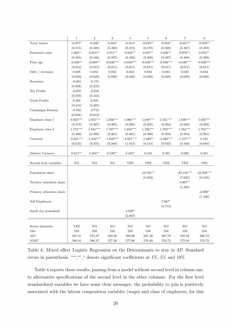
Table 4: Mixed effect Logistic Regression on the Determinants to stay in AP. Standard

errors in parenthesis. ∗∗∗,∗∗ ,∗ denote significant coefficients at 1%, 5% and 10%

Table 4 reports these results, passing from a model without second level in column one,

to alternative specifications of the second level in the other columns. For the first level

standardized variables we have some clear messages: the probability to join is positively

associated with the labour composition variables (wages and class of employees, for this

20

second one at a growing rate) and negatively associated with the assets and firm’s age,

while either the revenues or the dummy that controls for campaigns adopted in specific

districts of the city do not look significant in any specification. Among the sectors (results

are available upon request) a higher probability to join is associated with sector 4 and

with a significance close also to 10% sectors 7 and 9. The negative sign of assets could be

interpretated with a risky measure of the investment, while the firm’s age coefficient show

that on average, younger firms are more willing to declare their racket resistance. On the

other hand, firms with higher workforce are more likely to be joiners. Then, we observe

how there is a positive variance associated with the local level given by the districts. We

then, try to explain this, by looking to some district characteristics variables regarding

demography, human capital and labour market (there are not income data from the census

statistics) ranging from column 5 to column 8 (we don’t show all tests for non significant

variables). Our prior is, after the statistics presentation of the city characteristics that a

higher membership to the NGO is more associated with more educated districts, where

is easier to elicit the critical consumption behaviour. It means that the more populated

and poorer (given the quantity/quality demographic trade-off we showed before) districts

have, on average, less firms that join AP. We found, by using the selection criteria tests,

that the demography matters, either as small family percentage, or as population district

share (with opposite signs, as we stressed). Then, from this, labour market variables seem

do not affect this model, while education has a positive impact for primary and tertiary

completed education (even if the residual variance of column 8 disappears). The inclusion

of this second level variables improve also a little bit the selection criteria Akaike and

Modified Akaike, but most of all, it reduces the district variance.

5 Conclusions

This work used a new built database in order to assess the relevance of critical consumption

considerations in order to show acquiescence or resistance to organized crime racket.

Starting from the new unique experience of AddioPizzo, an NGO that tried to fight

extortion through critical consumption behaviour we built a database of firm and social

district characteristics for the city of Palermo in the period 2002-2012. This idea is linked

to the research fields of social mobility, customer discrimination, organized crime and is a

natural experiment to assess the role of human capital unconstrained with respect to the

institutions, given that the formal institution in the same city have to be the same. Our

results give a clear-cut picture of the situation, highlighting the dominant roles of economic

21

risk (proxied by the physical capital assets a firm belongs) and to the social behaviour

linked to the local expected reaction to the decision to show extortion resistance. This

latter point is proved by the strong statistical evidence that younger firms, with more

workforce, living in highly educated districts, have much higher probability to join. This

paper is also part of an open agenda, aimed also to measure the economic results implied

by this decision, that are the counterfactual gains or losses that firms decide to show this

resistance, tend to experience.

22

References

Akerlof, G., and J. Yellen, (1994) “Gang Behavior, Law Enforcement and Community

Values”, in Aaron, H.J, and T. E. Mann (Eds.), Values and Public Policy, Washington:

Brookings Institution.

Alexander, B. (1997). The Rational Racketeer: Pasta Protection in Depression Era

Chicago, The Journal of Law and Economics 40, 175-202.

Asmundo, A. & Lisciandra, M. (2008). The Cost of Protection Racket in Sicily, Global

Crime 9, 221-240.

Balletta, L. & Lavezzi, A.M. (2014). Extortion, Firm’s Size and the Sectoral Allocation

of Capital”, mimeo.

Battisti, M., Fioroni, T., Lavezzi, AM., Masserini, L. and M. Pratesi (2014), The Costs

and Benefits of Resisting the Extortion Racket, in progress.

Becker, G. (1957). The Economics of Discrimination. Chicago, University of

Chicago Press.

Browne W.J, & Draper, D. (2000). Implementation and performance issues in the Bayesian

and likelihood fitting of multilevel models. Computational Statistics , 15, 391-420.

Browne, W. J., & Draper, D. (2004). A comparison of Bayesian and like-

lihood methods for fitting multilevel models. Submitted. Downloadable from

http://multilevel.ioe.ac.uk/team/materials/wbrssa.pdf.

Bueno de Mesquita, E. & C. Hafer (2007). Public Protection or Private Extortion?, Eco-

nomics and Politics 20, 1-32.

Carlin, B. P. & Louis, T. A. (2000a). Bayes and Empirical Bayes Methods for

Data Analysis , 2nd edn. BocaRaton: Chapman and Hall-CRC.

Carlin, B. P. & Louis, T. A. (2000b.) Empirical Bayes: past, present and future. Journal

of America Statistical Association, 95, 1286-1289.

Clayton, D. G. (1996). Generalized linear mixed models . In: Gilks, W. R., Richard-

son, S., and Spiegelhalter, D. J. (eds), Markov chain Monte Carlo in practice. London:

Chapman and Hall.

23

Confesercenti (2010). XI Rapporto di Sos Impresa ”Le mani della criminalit sulle

imprese”. Confesercenti.

Congdon, P. (2006). Bayesian Models for Categorical Data. John Wiley and Sons,

New York.

De Leeuw, J., & Kreft, I. G. G. (1986). Random coefficient models for multilevel analysis.

Journal of Educational Statistics , 11, 57-85.

De Leeuw, J. & Meijer, E. (eds) (2008) Handbook of Multilevel Analysis. New York:

Springer.

Demidenko, E. (2004). Mixed Models. Theory and Applications . Hoboken, NJ:

Wiley.

Draper, D. (2008). Bayesian multilevel analysis and MCMC . In Handbook of

Quantitative Multilevel Analysis (de Leeuw J., editor). New York: Springer

Efron, B., & Morris, C. (1973). Stein’s estimation rule and its competitors - an empirical

Bayes approach, Journal of the American Statistical Association , 68, 117-130.

Efron, B., & Morris, C. (1975). Data analysis using Stein’s estimator and its generaliza-

tions, Journal of the American Statistical Association , 70, 311-319.

Forno, F. & Gunnarson, C. (2010) Everyday Shopping to Fight the Mafia in Italy, in

M. Micheletti and A. McFarland (eds.) Creative Participation: Responsibility-

taking in the Political World, London: Paradigm Publisher

Gambetta, D. (1993), The Sicilian Mafia: the Business of Private Protection,

Harvard University Press.

Gelfand, A. & Smith, A. (1990). Sampling-based approaches to calculating marginal den-

sities, Journal of the American Statistical Association 85, 398-409.

Gelman, A., & Hill, J. (2007). Data Analysis Using Regression And Multi-

level/Hierarchical Models. Cambridge, UK: Cambridge University Press

Glaeser, E. & Resseger, M.G. & Tobio, K. (2008). Urban Inequality, NBER Working

Paper Series WP 14419.

Goldstein, H.(2011). Multilevel Statistical Models, Wiley, New York.

24

Gunnarson, C. Changing the Game: Addiopizzo?s Mobilisation against Racketeering in

Palermo.

Hox, J.J.(2010). Multilevel Analysis: Techniques and Applications . 2nd edition.

New York: Routledge .

Jamieson, A. (2000). The Antimafia: Italy’s fight against organized crime. London:

Macmillan.

Konrad, K. A. & Skaperdas, S. (1998). Extortion, Economica 65, 461-477.

La Rosa, F., Paternostro, S, Picciotto, L. (2013), Determinants and Consquences of the

Anti-Mafia Entrepreneurial Behavior: an Empirical Study on Southern Italian Small-

Medium Enterprises, mimeo.

La Spina, A. (2008). Recent Anti-Mafia Strategies: the Italian Experience, in Siegel,

D. and H. Nelen (eds.), Organized Crime: Culture, Markets and Policies,

Springer.

Laird, N. M. & Ware, J. H. (1982). Random-Effects Models for longitudinal Data, Bio-

metrics , 38, 963-974.

Lavezzi, A. M. (2008). Economic Structure and Vulnerability to Organised Crime: Evi-

dence from Sicily, Global Crime 9, 198-220.

Lavezzi, A. M. (2014). Organised crime and the economy: a framework for policy pre-

scriptions, Global Crime , 15(1-2), 164-190.

Longford, N.T. (1987). A fast scoring algorithm for maximum likelihood estimation in

unbalanced mixed models with nested random effects, Biometrika , 74, 817-827.

Lotspeich, R. (1997). An Economic Analysis of Extortion in Russia, MOCT-MOST:

Economic Policy in Transitional Economies , 7, 21-53.

Maritz, J. S. & Lwin, T. (1989). Empirical Bayes Methods. London: Chapman and

Hall.

McCulloch, C.E.& Searle, S.R.& Neuhaus, J.M. (2008). Generalized, Linear, and

Mixed Models . New York: Wiley.

Morris, C. (1983). Parametric empirical Bayes inference, theory and applications, Jour-

nal of the American Statistical Association , 78, 47-65.

25

Paoli, L. (2003). Mafia Brotherhoods. Organized Crime, Italian Style, Oxford

University Press.

Partridge, H. (2012). The Determinants of and Barriers to Critical Consumption: A Study

of Addiopizzo, Modern Italy , 17(3).

Pinheiro, IC. & Bates, D.M. (1995). Approximations to the log-likelihood function in non-

linear mixed-effects models, Journal of Computational and Graphical Statis-

tics , 4, 12-35.

Rabe-Hesketh, S., & Skrondal, A. (2006). Multilevel modelling of complex survey data,

Journal of the Royal Statistical Society, Series A, 169, 805-827 .

Ramella, F. and C. Trigilia (1997), “Associazionismo e mobilitazione contro la criminalita

organizzata nel Mezzogiorno”, in Violante, L. (ed.), Mafia e societa italiana. Rapporto

1997, Laterza.

Raudenbush, S.W. & Bryk, A.S. (1986). A hierarchical model for studying school effects,

Sociology of Education , 59, 1-17.

Raudenbush, S.W. & Bryk, A.S. (1988). Methodological advances in studying effects of

schools and classrooms on student learning, Review of Research on Education ,

15, 423-476.

Raudenbush, S.W. & Bryk, A.S. (2002). Hierarchical Linear Models. Second Edition.

Sage Publications, Thousand Oaks.

Schelling, T. C. (1971), “What is the Business of Organized Crime?”, Journal of Public

Law 20, 71-84. Reprinted in T. C. Schelling (1984), Choice and Consequences, Harvard

University Press.

Schneider, J. C. & Schneider, P. T. (2003). Reversible Destiny. Mafia, Antimafia

and the Struggle for Palermo, University of California Press.

Skrondal, A. & Rabe-Hesketh, S. (2009). Prediction in multilevel generalised linear mod-

els, Journal of the Royal Statistical Society, Series A, 172(3), 659-687.

Snijders, T.A. & Bosker, R.(2011). Multilevel analysis. An introduction to basic

and advanced multilevel modelling . 2nd edition. Thousand Oaks, CA: Sage .

26

Tuerlinckx, F. & Rijmen, F. & Verbeke, G. & De Boeck, P. (2006). Statistical inference

in generalized linear mixed models: A review, British Journal of Mathematical

and Statistical Psychology , 59, 225-255.

Vaccaro, A. (2012). To pay or not to pay? Dynamic transparency and the fight against

the mafia?s extortionists. Journal of business ethics, 106(1), 23-35.

Vaccaro, A., & Palazzo, G. (2014). Values Against Violence. Institutional Change in

Societies Dominated by Organized Crime. Academy of Management Journal, amj-2012.

Varese, F. (2001). The Russian Mafia: Private Protection in a New Market

Economy: Private Protection in a New Market Economy. Oxford University

Press.

Varese, F. (2006). How Mafias Migrate: The Case of the‘Ndrangheta in Northern Italy,

Law and Society Review 40, 411-444.

Varese, F. (2014). Protection and Extortion, Oxford Handbook of Organized Crime ,

343-58.

Tables

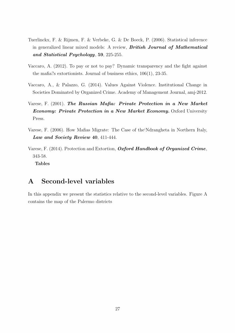
A Second-level variables

In this appendix we present the statistics relative to the second-level variables. Figure A

contains the map of the Palermo districts

27

Table 5: Palermo districts: map

ID District name

1 Partanna Mondello

2 Tommaso Natale

3 Pallavicino

4 Monte Pellegrino

5 Arenella Vergine Maria

6 Resuttano San Lorenzo

7 Cruillas CEP

8 Borgo Nuovo

9 Uditore - Passo di Rigano

10 Malaspina-Palagonia

11 Liberta’

12 Politeama

13 Noce

14 Boccadifalco

15 Altarello

16 Zisa

17 Palazzo Reale - Monte di Pieta’

18 Tribunali-Castellammare

19 Cuba-Calatafimi

20 Mezzomonreale

21 Santa Rosalia

22 Oreto

23 Settecannoli

24 Brancaccio-Ciaculli

25 Villagrazia-Falsomiele

Table 6: Palermo districts: names

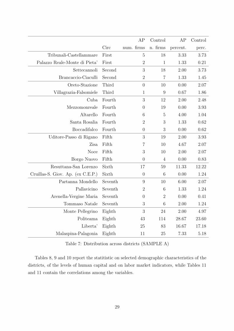
Table 5 contains the distribution of the AP firms and the control group across the

districts.

28

AP Control AP Control

Circ num. firms n. firms percent. perc.

Tribunali-Castellammare First 5 18 3.33 3.73

Palazzo Reale-Monte di Pieta’ First 2 1 1.33 0.21

Settecannoli Second 3 18 2.00 3.73

Brancaccio-Ciaculli Second 2 7 1.33 1.45

Oreto-Stazione Third 0 10 0.00 2.07

Villagrazia-Falsomiele Third 1 9 0.67 1.86

Cuba Fourth 3 12 2.00 2.48

Mezzomonreale Fourth 0 19 0.00 3.93

Altarello Fourth 6 5 4.00 1.04

Santa Rosalia Fourth 2 3 1.33 0.62

Boccadifalco Fourth 0 3 0.00 0.62

Uditore-Passo di Rigano Fifth 3 19 2.00 3.93

Zisa Fifth 7 10 4.67 2.07

Noce Fifth 3 10 2.00 2.07

Borgo Nuovo Fifth 0 4 0.00 0.83

Resuttana-San Lorenzo Sixth 17 59 11.33 12.22

Cruillas-S. Giov. Ap. (ex C.E.P.) Sixth 0 6 0.00 1.24

Partanna Mondello Seventh 9 10 6.00 2.07

Pallavicino Seventh 2 6 1.33 1.24

Arenella-Vergine Maria Seventh 0 2 0.00 0.41

Tommaso Natale Seventh 3 6 2.00 1.24

Monte Pellegrino Eighth 3 24 2.00 4.97

Politeama Eighth 43 114 28.67 23.60

Liberta’ Eighth 25 83 16.67 17.18

Malaspina-Palagonia Eighth 11 25 7.33 5.18

Table 7: Distribution across districts (SAMPLE A)

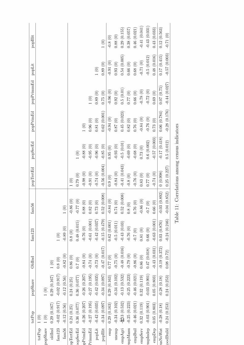
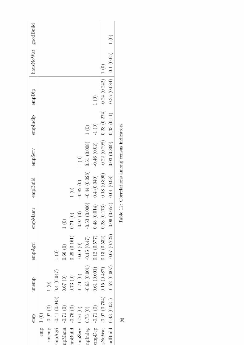
Tables 8, 9 and 10 report the statitistic on selected demographic characteristics of the

districts, of the levels of human capital and on labor market indicators, while Tables 11

and 11 contain the correlations among the variables.

29

Circ Tot. Pop. Depend. Ratio Family 123 Family 56

Palazzo Reale-Monte di Pieta’ First 11352 0.69 0.71 0.12

Tribunali-Castellammare First 10137 0.86 0.73 0.12

Brancaccio-Ciaculli Second 15618 0.45 0.54 0.18

Settecannoli Second 52481 0.56 0.54 0.18

Oreto-Stazione Third 42504 0.89 0.64 0.13

Villagrazia-Falsomiele Third 40915 0.62 0.56 0.17

Altarello Fourth 16944 0.53 0.57 0.15

Boccadifalco Fourth 7909 0.47 0.59 0.16

Cuba Fourth 23587 0.91 0.63 0.12

Mezzomonreale Fourth 38567 0.7 0.58 0.14

Santa Rosalia Fourth 25678 1.03 0.64 0.13

Borgo Nuovo Fifth 21085 0.74 0.56 0.2

Noce Fifth 29940 0.95 0.67 0.11

Uditore-Passo di Rigano Fifth 33331 0.88 0.63 0.12

Zisa Fifth 36260 0.89 0.63 0.13

Cruillas-S. Giov. Ap. (ex C.E.P.) Sixth 32998 0.54 0.55 0.15

Resuttana-San Lorenzo Sixth 45376 1.34 0.7 0.07

Arenella-Vergine Maria Seventh 9299 0.64 0.59 0.15

Pallavicino Seventh 27428 0.48 0.55 0.19

Partanna Mondello Seventh 16652 0.77 0.68 0.09

Tommaso Natale Seventh 21125 0.54 0.59 0.14

Liberta’ Eighth 45002 1.6 0.75 0.06

Malaspina-Palagonia Eighth 21793 1.88 0.74 0.06

Monte Pellegrino Eighth 29011 0.86 0.65 0.12

Politeama Eighth 31730 1.18 0.73 0.08

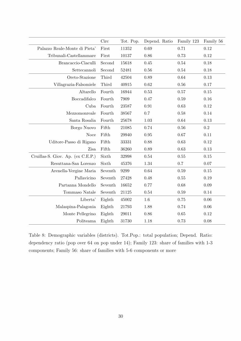
Table 8: Demographic variables (districts). Tot.Pop.: total population; Depend. Ratio:

dependency ratio (pop over 64 on pop under 14); Family 123: share of families with 1-3

components; Family 56: share of families with 5-6 components or more

30

Circ Primm. Ed. Prim. Ed. Sec. Ed. Tert. Ed. Pop. Lit. Pop. Illit.

Palazzo Reale-Monte di Pieta’ First 0.32 0.61 0.11 0.05 0.17 0.06

Tribunali-Castellammare First 0.27 0.54 0.16 0.1 0.16 0.05

Brancaccio-Ciaculli Second 0.31 0.65 0.15 0.02 0.15 0.03

Settecannoli Second 0.3 0.65 0.16 0.02 0.14 0.03

Oreto-Stazione Third 0.29 0.61 0.2 0.05 0.12 0.03

Villagrazia-Falsomiele Third 0.28 0.62 0.21 0.03 0.12 0.02

Altarello Fourth 0.29 0.66 0.16 0.02 0.13 0.02

Boccadifalco Fourth 0.23 0.58 0.21 0.06 0.12 0.02

Cuba Fourth 0.24 0.55 0.26 0.07 0.1 0.02

Mezzomonreale Fourth 0.22 0.56 0.28 0.06 0.09 0.01

Santa Rosalia Fourth 0.28 0.61 0.2 0.05 0.11 0.03

Borgo Nuovo Fifth 0.31 0.67 0.13 0.02 0.13 0.04

Noce Fifth 0.27 0.59 0.21 0.06 0.11 0.02

Uditore-Passo di Rigano Fifth 0.21 0.51 0.29 0.1 0.09 0.01

Zisa Fifth 0.27 0.6 0.2 0.06 0.11 0.02

Cruillas-S. Giov. Ap. (ex C.E.P.) Sixth 0.24 0.57 0.25 0.04 0.11 0.03

Resuttana-San Lorenzo Sixth 0.13 0.34 0.39 0.2 0.06 0.01

Arenella-Vergine Maria Seventh 0.29 0.64 0.19 0.03 0.12 0.01

Pallavicino Seventh 0.31 0.63 0.15 0.04 0.14 0.03

Partanna Mondello Seventh 0.2 0.47 0.3 0.12 0.09 0.01

Tommaso Natale Seventh 0.22 0.56 0.25 0.07 0.11 0.02

Liberta’ Eighth 0.11 0.3 0.35 0.29 0.06 0

Malaspina-Palagonia Eighth 0.14 0.34 0.37 0.23 0.06 0

Monte Pellegrino Eighth 0.24 0.53 0.27 0.08 0.1 0.02

Politeama Eighth 0.18 0.41 0.26 0.21 0.1 0.02

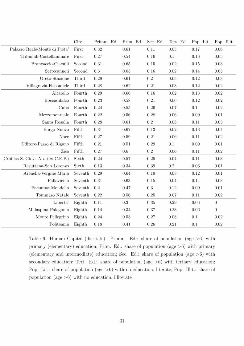
Table 9: Human Capital (districts). Primm. Ed.: share of population (age >6) with

primary (elementary) education; Prim. Ed.: share of population (age >6) with primary

(elementary and intermediate) education; Sec. Ed.: share of population (age >6) with

secondary education; Tert. Ed.: share of population (age >6) with tertiary education;

Pop. Lit.: share of population (age >6) with no education, literate; Pop. Illit.: share of

population (age >6) with no education, illiterate

31

32

Cir

cE

mp

l.U

nem

pl.

Em

pl.

Agr

.E

mp

l.M

anu

fE

mp

l.C

onst

r.E

mp

l.S

erv.

Em

pl.

Dep

.E

mp

l.In

dep

.

Pala

zzo

Rea

le-M

onte

di

Pie

ta’

Fir

st0.

540.

270.

020.

090.

070.

820.8

30.1

6

Tri

bu

nal

i-C

aste

llam

mar

eF

irst

0.68

0.19

0.03

0.1

0.05

0.81

0.7

60.2

3

Bra

nca

ccio

-Cia

cull

iS

econ

d0.

60.

20.

060.

150.

070.

710.8

30.1

5

Set

teca

nn

oli

Sec

ond

0.6

0.2

0.03

0.13

0.06

0.76

0.8

30.1

6

Ore

to-S

tazi

one

Th

ird

0.65

0.19

0.02

0.12

0.06

0.79

0.8

30.1

5

Vil

lagr

azia

-Fal

som

iele

Th

ird

0.66

0.17

0.03

0.11

0.06

0.78

0.8

20.1

7

Alt

arel

loF

ourt

h0.

620.

20.

020.

130.

080.

750.8

40.1

5

Bocc

adif

alco

Fou

rth

0.65

0.16

0.01

0.1

0.09

0.78

0.8

10.1

7

Cu

ba

Fou

rth

0.72

0.15

0.02

0.09

0.04

0.83

0.8

30.1

6

Mez

zom

onre

ale

Fou

rth

0.72

0.14

0.02

0.09

0.05

0.83

0.8

20.1

7

San

taR

osal

iaF

ourt

h0.

640.

180.

020.

090.

050.

830.8

50.1

4

Bor

goN

uov

oF

ifth

0.59

0.21

0.02

0.13

0.08

0.75

0.8

50.1

3

Noce

Fif

th0.

670.

170.

020.

10.

060.

810.8

20.1

7

Ud

itore

-Pas

sod

iR

igan

oF

ifth

0.74

0.14

0.01

0.08

0.05

0.84

0.8

10.1

8

Zis

aF

ifth

0.64

0.17

0.01

0.09

0.06

0.83

0.8

20.1

7

Cru

illa

s-S

.G

iov.

Ap

.(e

xC

.E.P

.)S

ixth

0.68

0.18

0.02

0.11

0.07

0.79

0.8

30.1

6

Res

utt

ana-

San

Lor

enzo

Six

th0.

860.

080.

010.

070.

040.

860.7

80.2

2

Are

nel

la-V

ergi

ne

Mar

iaS

even

th0.

670.

160.

030.

150.

060.

740.8

0.1

8

Pal

lavic

ino

Sev

enth

0.59

0.21

0.02

0.12

0.07

0.77

0.8

20.1

7

Part

an

na

Mon

del

loS

even

th0.

770.

140.

020.

080.

060.

820.7

0.2

9

Tom

mas

oN

atal

eS

even

th0.

70.

170.

030.

140.

070.

750.7

70.2

2

Lib

erta

’E

ighth

0.87

0.07

0.01

0.05

0.03

0.89

0.7

50.2

5

Mal

asp

ina-

Pal

agon

iaE

ighth

0.86

0.07

0.01

0.05

0.03

0.9

0.7

70.2

2

Monte

Pel

legr

ino

Eig

hth

0.73

0.15

0.01

0.12

0.05

0.8

0.8

10.1

8

Pol

itea

ma

Eig

hth

0.82

0.1

0.02

0.07

0.04

0.87

0.7

30.2

6

Tab

le10

:L

abor

Mar

ket

indic

ator

s(d

istr

icts

).E

mpl.:

emplo

ym

ent

rate

;U

nem

pl.:

emplo

ym

ent

rate

;E

mpl.

Agr

.:sh

are

ofem

pl.

inA

gric

oltu

re;

Em

pl.

Man

uf.

:sh

are

ofem

pl.

inM

anif

actu

re;

Em

pl.

Con

str.

:sh

are

ofem

pl.

inC

onst

ruct

ion;

Em

pl.

Dep

.:sh

are

ofem

plo

yees

;E

mpl.

Indep

.:sh

are

ofse

lf-e

mplo

yed

33

totP

opp

opS

har

eO

ldIn

dfa

m12

3fa

m56

pop

Ter

tEd

pop

Sec

Ed

pop

Pri

mE

dp

op

Pri

mm

Ed

pop

Lit

pop

Illi

t

totP

op1

(0)

pop

Sh

are

1(0

)1

(0)

old

Ind

0.29

(0.1

67)

0.29

(0.1

67)

1(0

)

fam

123

-0.0

2(0

.917

)-0

.02

(0.9

17)

0.8

(0)

1(0

)

fam

56-0

.12

(0.5

6)-0

.12

(0.5

6)-0

.82

(0)

-0.8

9(0

)1

(0)

pop

Ter

tEd

0.24

(0.2

5)0.

24(0

.25)

0.86

(0)

0.8

(0)

-0.8

6(0

)1

(0)

pop

Sec

Ed

0.36

(0.0

77)

0.36

(0.0

77)

0.7

(0)

0.48

(0.0

15)

-0.7

7(0

)0.7

9(0

)1

(0)

pop

Pri

mE

d-0

.26

(0.2

07)

-0.2

6(0

.207

)-0

.84

(0)

-0.7

6(0

)0.

88

(0)

-0.9

8(0

)-0

.88

(0)

1(0

)

pop

Pri

mm

Ed

-0.2

7(0

.195

)-0

.27

(0.1

95)

-0.7

4(0

)-0

.61

(0.0

01)

0.82

(0)

-0.9

1(0

)-0

.95

(0)

0.9

6(0

)1

(0)

pop

Lit

-0.4

2(0

.035

)-0

.42

(0.0

35)

-0.7

3(0

)-0

.42

(0.0

37)

0.73

(0)

-0.7

4(0

)-0

.96

(0)

0.8

1(0

)0.8

9(0

)1

(0)

pop

Illi

t-0

.34

(0.0

97)

-0.3

4(0

.097

)-0

.47

(0.0

17)

-0.1

5(0

.479

)0.

52

(0.0

08)

-0.5

6(0

.004)

-0.8

5(0

)0.6

2(0

.001)

0.75

(0)

0.8

9(0

)1

(0)

emp

0.29

(0.1

63)

0.29

(0.1

63)

0.77

(0)

0.62

(0.0

01)

-0.8

4(0

)0.9

(0)

0.9

5(0

)-0

.94

(0)

-0.9

6(0

)-0

.91

(0)

-0.8

(0)

un

emp

-0.3

4(0

.102

)-0

.34

(0.1

02)

-0.7

5(0

)-0

.5(0

.011

)0.

74

(0)

-0.8

4(0

)-0

.93

(0)

0.8

7(0

)0.9

2(0

)0.9

3(0

)0.8

8(0

)

emp

Agr

i-0

.13

(0.5

32)

-0.1

3(0

.532

)-0

.48

(0.0

16)

-0.4

3(0

.03)

0.52

(0.0

08)

-0.4

1(0

.043)

-0.5

(0.0

1)

0.4

5(0

.023)

0.5

(0.0

1)

0.5

4(0

.005)

0.2

9(0

.155)

emp

Man

u-0

.25

(0.2

23)

-0.2

5(0

.223

)-0

.79

(0)

-0.7

6(0

)0.

8(0

)-0

.8(0

)-0

.69

(0)

0.8

2(0

)0.

77

(0)

0.6

6(0

)0.3

8(0

.057)

emp

Bu

il-0

.46

(0.0

21)

-0.4

6(0

.021

)-0

.86

(0)

-0.7

(0)

0.76

(0)

-0.7

6(0

)-0

.68

(0)

0.7

6(0

)0.6

6(0

)0.6

8(0

)0.4

6(0

.021)

emp

Ser

v0.

32(0

.119

)0.

32(0

.119

)0.

86(0

)0.

81(0

)-0

.86

(0)

0.8

3(0

)0.7

3(0

)-0

.84

(0)

-0.7

8(0

)-0

.71

(0)

-0.4

1(0

.041)

emp

Ind

ep-0

.03

(0.9

01)

-0.0

3(0

.901

)0.

47(0

.018

)0.

66(0

)-0

.7(0

)0.7

7(0

)0.6

(0.0

02)

-0.7

6(0

)-0

.72

(0)

-0.5

(0.0

12)

-0.4

3(0

.031)

emp

Dep

0.05

(0.8

03)

0.05

(0.8

03)

-0.4

3(0

.031

)-0

.63

(0.0

01)

0.66

(0)

-0.7

4(0

)-0

.57

(0.0

03)

0.7

3(0

)0.6

9(0

)0.4

8(0

.016)

0.4

3(0

.033)

hou

sNoW

at-0

.28

(0.1

8)-0

.28

(0.1

8)-0

.19

(0.3

72)

0.03

(0.8

76)

-0.0

3(0

.892)

0(0

.998)

-0.1

7(0

.418)

0.0

6(0

.784)

0.0

7(0

.75)

0.1

7(0

.415)

0.1

2(0

.563)

good

Bu

ild

0.24

(0.2

53)

0.24

(0.2

53)

0.08

(0.7

2)-0

.24

(0.2

46)

-0.0

4(0

.852)

0.2

5(0

.227)

0.5

(0.0

12)

-0.2

8(0

.176)

-0.4

4(0

.027)

-0.5

7(0

.003)

-0.7

1(0

)

Tab

le11

:C

orre

lati

ons

amon

gce

nsu

sin

dic

ator

s

34

emp

unem

pem

pA

gri

empM

anu

empB

uild

empSer

vem

pIn

dip

empD

iphou

sNoW

atgo

odB

uild

emp

1(0

)

unem

p-0

.97

(0)

1(0

)

empA

gri

-0.4

1(0

.043

)0.

4(0

.047

)1

(0)

empM

anu

-0.7

1(0

)0.

67(0

)0.

66(0

)1

(0)

empB

uild

-0.7

6(0

)0.

73(0

)0.

29(0

.161

)0.

71(0

)1

(0)

empSer

v0.

76(0

)-0

.71

(0)

-0.6

9(0

)-0

.97

(0)

-0.8

2(0

)1

(0)

empIn

dep

0.73

(0)

-0.6

3(0

.001

)-0

.15

(0.4

7)-0

.53

(0.0

06)

-0.4

4(0

.028

)0.

51(0

.008

)1

(0)

empD

ep-0

.71

(0)

0.61

(0.0

01)

0.12

(0.5

77)

0.48

(0.0

14)

0.4

(0.0

49)

-0.4

6(0

.02)

-1(0

)1

(0)

hou

sNoW

at-0

.07

(0.7

54)

0.15

(0.4

87)

0.13

(0.5

32)

0.28

(0.1

73)

0.18

(0.3

95)

-0.2

2(0

.298

)0.

23(0

.274

)-0

.24

(0.2

42)

1(0

)

goodB

uild

0.43

(0.0

31)

-0.5

2(0

.007

)-0

.07

(0.7

25)

-0.0

9(0

.654

)0.

01(0

.98)

0.03

(0.8

69)

0.33

(0.1

1)-0

.35

(0.0

84)

-0.1

(0.6

5)1

(0)

Tab

le12

:C

orre

lati

ons

amon

gce

nsu

sin

dic

ator

s

35