Embed Size (px)
Citation preview

Liu, X., Zhang, L. "Structural Theory." Bridge Engineering Handbook. Ed. Wai-Fah Chen and Lian Duan Boca Raton: CRC Press, 2000
7Structural Theory
Co nstitutive Law • Three Levels: Continuous Mechanics, Finite-Element Method, Beam–Column Theory • Theoretical Structural Mechanics, Computational Structural Mechanics, and Qualitative Structural Mechanics • Matrix Analysis of Structures: Force Method and Displacement Method
7.2 Equilibrium Equations
Equilibrium Equation and Virtual Work Equation • Equilibrium Equation for Elements • Coordinate Transformation • Equilibrium Equation for Structures • Influence Lines and Surfaces
7.3 Compatibility Equations
Large Deformation and Large Strain • Compatibility Equation for Elements • Compatibility Equation for Structures • Contragredient Law
7.4 Constitutive Equations
Elasticity and Plasticity • Linear Elastic and Nonlinear Elastic Behavior • Geometric Nonlinearity
7.5 Displacement Method
Stiffness Matrix for Elements • Stiffness Matrix for Structures • Matrix Inversion • Special Consideration
7.6 Substructuring and Symmetry Consideration
7.1 Introduction
In this chapter, general forms of three sets of equations required in solving a solid mechanics problemand their extensions into structural theory are presented. In particular, a more generally usedmethod, displacement method, is expressed in detail.
7.1.1 Basic Equations: Equilibrium, Compatibility, and Constitutive Law
In general, solving a solid mechanics problem must satisfy equations of equilibrium (static ordynamic), conditions of compatibility between strains and displacements, and stress–strain relationsor material constitutive law (see Figure 7.1). The initial and boundary conditions on forces anddisplacements are naturally included.
From consideration of equilibrium equations, one can relate the stresses inside a body to externalexcitations, including body and surface forces. There are three equations of equilibrium relating the
Xila LiuTsinghua University, China
Leiming ZhangTsinghua University, China
7.1 IntroductionBasic Equations: Equilibrium, Compatibility, and
© 2000 by CRC Press LLC
six components of stress tensor for an infinitesimal material element which will be shown laterin Section 7.2.1. In the case of dynamics, the equilibrium equations are replaced by equations ofmotion, which contain second-order derivatives of displacement with respect to time.
In the same way, taking into account geometric conditions, one can relate strains inside a bodyto its displacements, by six equations of kinematics expressing the six components of strain ( )in terms of the three components of displacement ( ). These are known as the strain–displacementrelations (see Section 7.3.1).
Both the equations of equilibrium and kinematics are valid regardless of the specific material ofwhich the body is made. The influence of the material is expressed by constitutive laws in sixequations. In the simplest case, not considering the effects of temperature, time, loading rates, andloading paths, these can be described by relations between stress and strain only.
Six stress components, six strain components, and three displacement components are connectedby three equilibrium equations, six kinematics equations, and six constitutive equations. The 15unknown quantities can be determined from the system of 15 equations.
It should be pointed out that the principle of superposition is valid only when small deformationsand elastic materials are assumed.
7.1.2 Three Levels: Continuous Mechanics, Finite–Element Method, Beam–Column Theory
In solving a solid mechanics problem, the most direct method solves the three sets of equationsdescribed in the previous section. Generally, there are three ways to establish the basic unknowns,namely, the displacement components, the stress components, or a combination of both. Thecorresponding procedures are called the displacement method, the stress method, or the mixedmethod, respectively. But these direct methods are only practicable in some simple circumstances,such as those detailed in elastic theory of solid mechanics.
Many complex problems cannot be easily solved with conventional procedures. Complexitiesarise due to factors such as irregular geometry, nonhomogeneities, nonlinearity, and arbitraryloading conditions. An alternative now available is based on a concept of discretization. The finite-element method (FEM) divides a body into many “small” bodies called finite elements. Formulationsby the FEM on the laws and principles governing the behavior of the body usually result in a setof simultaneous equations that can be solved by direct or iterative procedures. And loading effectssuch as deformations and stresses can be evaluated within certain accuracy. Up to now, FEM hasbeen the most widely used structural analysis method.
In dealing with a continuous beam, the size of the three sets of equations is greatly reduced byassuming characteristics of beam members such as plane sections remain plane. For framed structures
FIGURE 7.1 Relations of variables in solving a solid mechanics problem.
σij
εij
ui
© 2000 by CRC Press LLC
or structures constructed using beam–columns, structural mechanics gives them a more pithy andpractical analysis.
7.1.3 Theoretical Structural Mechanics, Computational Structural Mechanics, and Qualitative Structural Mechanics
Structural mechanics deals with a system of members connected by joints which may be pinned orrigid. Classical methods of structural analysis are based on principles such as the principle of virtualdisplacement, the minimization of total potential energy, the minimization of total complementaryenergy, which result in the three sets of governing equations. Unfortunately, conventional methodsare generally intended for hand calculations and developers of the FEM took great pains to minimizethe amount of calculations required, even at the expense of making the methods somewhat unsys-tematic. This made the conventional methods unattractive for translation to computer codes.
The digital computer called for a more systematic method of structural analysis, leading to compu-tational structural mechanics. By taking great care to formulate the tools of matrix notation in amathematically consistent fashion, the analyst achieved a systematic approach convenient for automaticcomputation: matrix analysis of structures. One of the hallmarks of structural matrix analysis is itssystematic nature, which renders digital computers even more important in structural engineering.
Of course, the analyst must maintain a critical, even skeptical, attitude toward computer results.In any event, computer results must satisfy our intuition of what is “reasonable.” This qualitativejudgment requires that the analyst possess a full understanding of structural behavior, both thatbeing modeled by the program and that which can be expected in the actual structures. Engineersshould decide what approximations are reasonable for the particular structure and verify that theseapproximations are indeed valid, and know how to design the structure so that its behavior is inreasonable agreement with the model adopted to analyze it. This is the main task of a structuralanalyst.
7.1.4 Matrix Analysis of Structures: Force Method and Displacement Method
Matrix analysis of structures was developed in the early 1950s. Although it was initially used onfuselage analysis, this method was proved to be pertinent to any complex structure. If internal forcesare selected as basic unknowns, the analysis method is referred to as force method; in a similar way,the displacement method refers to the case where displacements are selected as primary unknowns.Both methods involve obtaining the joint equilibrium equations in terms of the basic internal forcesor joint displacements as primary unknowns and solving the resulting set of equations for theseunknowns. Having done this, one can obtain internal forces by backsubstitution, since even in thecase of the displacement method the joint displacements determine the basic displacements of eachmember, which are directly related to internal forces and stresses in the member.
A major feature evident in structural matrix analysis is an emphasis on a systematic approach tothe statement of the problem. This systematic characteristic together with matrix notation makesit especially convenient for computer coding. In fact, the displacement method, whose basicunknowns are uniquely defined, is generally more convenient than the force method. Most general-purpose structural analysis programs are displacement based. But there are still cases where it maybe more desirable to use the force method.
7.2 Equilibrium Equations
7.2.1 Equilibrium Equation and Virtual Work Equation
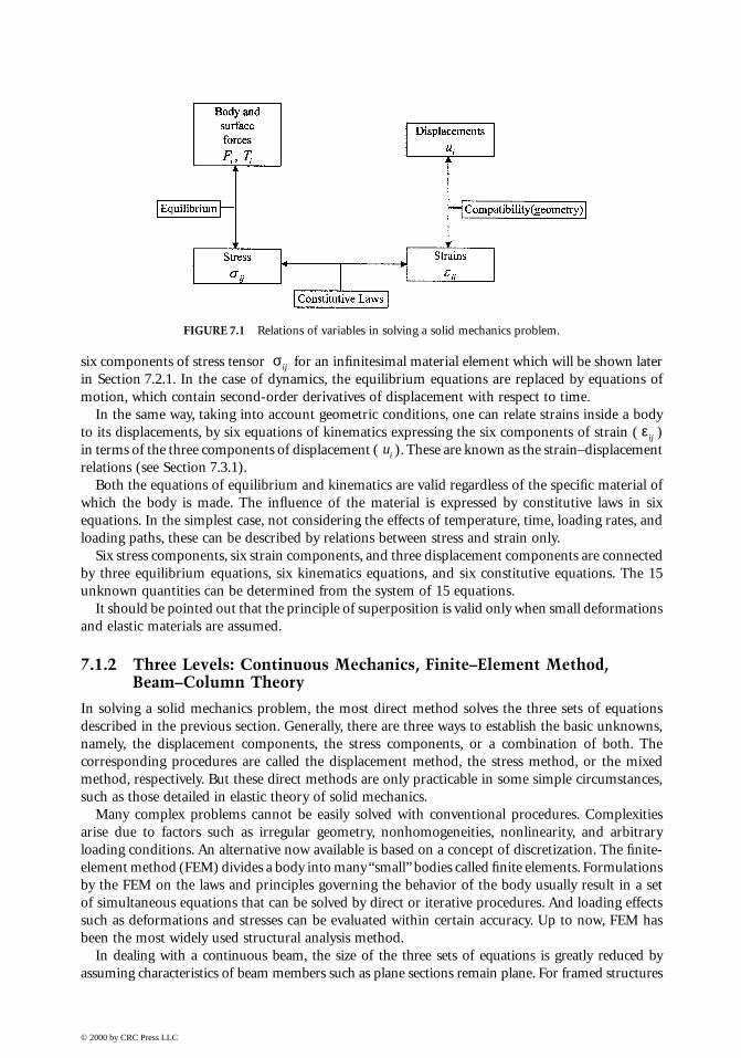
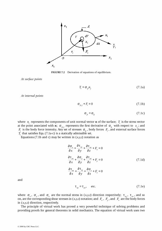
For any volume V of a material body having A as surface area, as shown in Figure 7.2, it has thefollowing conditions of equilibrium:
© 2000 by CRC Press LLC
At surface points
(7.1a)
At internal points
(7.1b)
(7.1c)
where represents the components of unit normal vector n of the surface; is the stress vectorat the point associated with n; represents the first derivative of with respect to ; and
is the body force intensity. Any set of stresses , body forces , and external surface forces that satisfies Eqs. (7.1a-c) is a statically admissible set.Equations (7.1b and c) may be written in (x,y,z) notation as
(7.1d)
and
etc. (7.1e)
where , , and are the normal stress in (x,y,z) direction respectively; , , and soon, are the corresponding shear stresses in (x,y,z) notation; and , , and are the body forcesin (x,y,z) direction, respectively.
The principle of virtual work has proved a very powerful technique of solving problems andproviding proofs for general theorems in solid mechanics. The equation of virtual work uses two
FIGURE 7.2 Derivation of equations of equilibrium.
T ni ji j= σ
σ ji j iF, + = 0
σ σji ij=
ni Ti
σ ji j, σij x j
Fi σij Fi
Ti
∂σ∂
∂τ∂
∂τ∂
∂τ∂
∂σ∂
∂τ∂
∂τ∂
∂τ∂
∂σ∂
x xy xzx
yx y yzy
zx zy zz
x y zF
x y zF
x y zF
+ + + =
+ + + =
+ + + =
0
0
0
τ τxy yx= ,
σx σy σz τ xy τ yx
Fx Fy Fz
© 2000 by CRC Press LLC
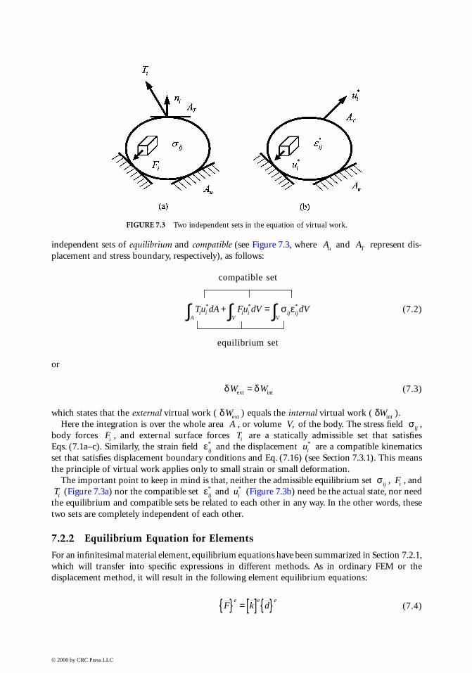
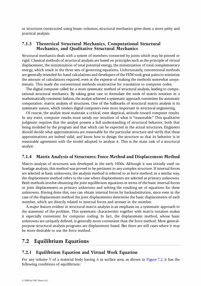
independent sets of equilibrium and compatible (see Figure 7.3, where and represent dis-placement and stress boundary, respectively), as follows:
compatible set
(7.2)
equilibrium set
or
(7.3)
which states that the external virtual work ( ) equals the internal virtual work ( ).Here the integration is over the whole area , or volume of the body. The stress field ,
body forces , and external surface forces are a statically admissible set that satisfiesEqs. (7.1a–c). Similarly, the strain field and the displacement are a compatible kinematicsset that satisfies displacement boundary conditions and Eq. (7.16) (see Section 7.3.1). This meansthe principle of virtual work applies only to small strain or small deformation.
The important point to keep in mind is that, neither the admissible equilibrium set , , and (Figure 7.3a) nor the compatible set and (Figure 7.3b) need be the actual state, nor need
the equilibrium and compatible sets be related to each other in any way. In the other words, thesetwo sets are completely independent of each other.
7.2.2 Equilibrium Equation for Elements
For an infinitesimal material element, equilibrium equations have been summarized in Section 7.2.1,which will transfer into specific expressions in different methods. As in ordinary FEM or thedisplacement method, it will result in the following element equilibrium equations:
(7.4)
FIGURE 7.3 Two independent sets in the equation of virtual work.
Au AT
Tu dA Fu dV dVi iA
i iV
ij ijV
* * *∫ ∫ ∫+ = σ ε
δ δW Wext = int
δWext δWint
A V, σij
Fi Ti
εij* ui
*
σij Fi
Ti εij* ui
*
F k de e e{ } = [ ] { }
© 2000 by CRC Press LLC
where and are the element nodal force vector and displacement vector, respectively, while is element stiffness matrix; the overbar here means in local coordinate system.
In the force method of structural analysis, which also adopts the idea of discretization, it is provedpossible to identify a basic set of independent forces associated with each member, in that not onlyare these forces independent of one another, but also all other forces in that member are directlydependent on this set. Thus, this set of forces constitutes the minimum set that is capable ofcompletely defining the stressed state of the member. The relationship between basic and local forcesmay be obtained by enforcing overall equilibrium on one member, which gives
(7.5)
where = the element force transformation matrix and = the element primary forcesvector. It is important to emphasize that the physical basis of Eq. (7.5) is member overall equilibrium.
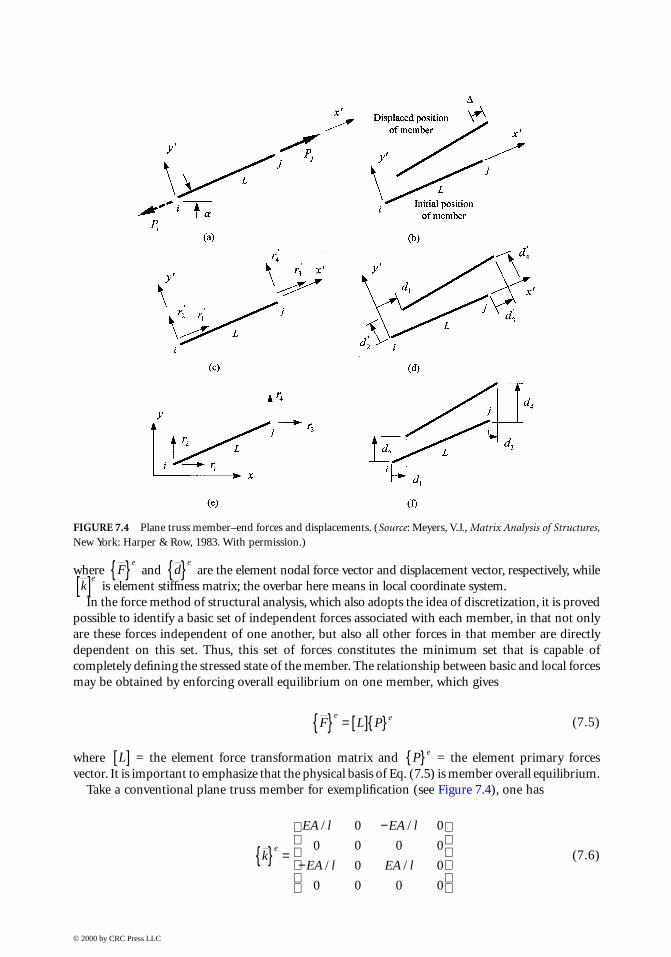
Take a conventional plane truss member for exemplification (see Figure 7.4), one has
(7.6)
FIGURE 7.4 Plane truss member–end forces and displacements. (Source: Meyers, V.J., Matrix Analysis of Structures,New York: Harper & Row, 1983. With permission.)
Fe{ } d
e{ }k
e[ ]
F L Pe e{ } = [ ]{ }
L[ ] P e{ }
k
EA l EA l
EA l EA l
e{ } =
−
−
/ /
/ /
0 0
0 0 0 0
0 0
0 0 0 0
© 2000 by CRC Press LLC
and
(7.7)
where EA/l = axial stiffness of the truss member and P = axial force of the truss member.
7.2.3 Coordinate Transformation
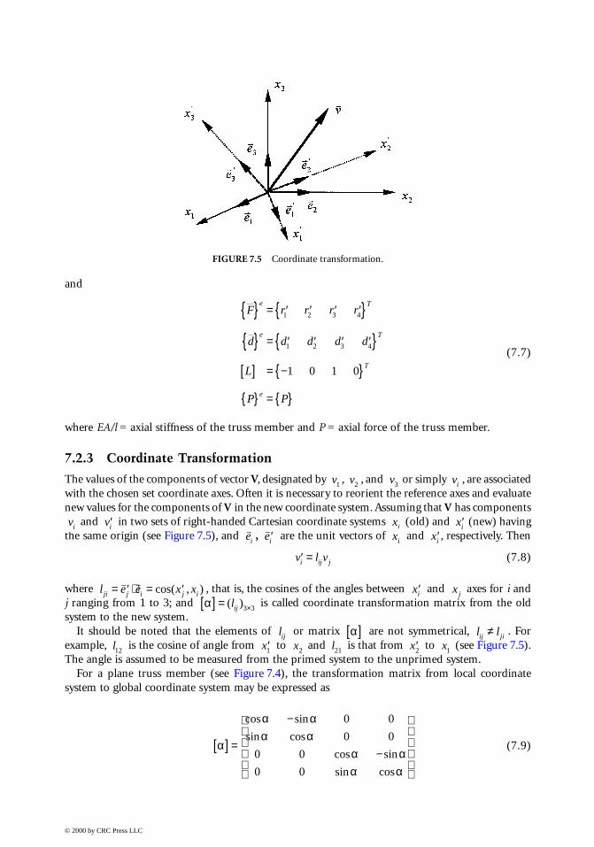
The values of the components of vector V, designated by , , and or simply , are associatedwith the chosen set coordinate axes. Often it is necessary to reorient the reference axes and evaluatenew values for the components of V in the new coordinate system. Assuming that V has components
and in two sets of right-handed Cartesian coordinate systems (old) and (new) havingthe same origin (see Figure 7.5), and , are the unit vectors of and , respectively. Then
(7.8)
where , that is, the cosines of the angles between and axes for i andj ranging from 1 to 3; and is called coordinate transformation matrix from the oldsystem to the new system.
It should be noted that the elements of or matrix are not symmetrical, . Forexample, is the cosine of angle from to and is that from to (see Figure 7.5).The angle is assumed to be measured from the primed system to the unprimed system.
For a plane truss member (see Figure 7.4), the transformation matrix from local coordinatesystem to global coordinate system may be expressed as
(7.9)
FIGURE 7.5 Coordinate transformation.
F r r r r
d d d d d
L
P P
e T
e T
T
e
{ } = ′ ′ ′ ′{ }
{ } = ′ ′ ′ ′{ }[ ] = −{ }
{ } = { }
1 2 3 4
1 2 3 4
1 0 1 0
v1 v2 v3 vi
vi ′vi xi ′xi
vei
v′ei xi ′xi
′ =v l vi ij j
l e e x xji j i j i= ′ ⋅ = ′v v
cos( , ) ′xi x j
α[ ] = ×( )lij 3 3
lij α[ ] l lij ji≠l12 ′x1 x2 l21 ′x2 x1
α
α αα α
α αα α
[ ] =
−
−
cos sin
sin cos
cos sin
sin cos
0 0
0 0
0 0
0 0
© 2000 by CRC Press LLC
where α is the inclined angle of the truss member which is assumed to be measured from the globalto the local coordinate system.
7.2.4 Equilibrium Equation for Structures
For discretized structure, the equilibrium of the whole structure is essentially the equilibrium ofeach joint. After assemblage,
For ordinary FEM or displacement method
(7.10)
For force method
(7.11)
where = nodal loading vector; = total stiffness matrix; = nodal displacement vector; = total forces transformation matrix; = total primary internal forces vector.
It should be noted that the coordinate transformation for each element from local coordinatesto the global coordinate system must be done before assembly.
In the force method, Eq. (7.11) will be adopted to solve for internal forces of a statically deter-minate structure. The number of basic unknown forces is equal to the number of equilibriumequations available to solve for them and the equations are linearly independent. For staticallyunstable structures, analysis must consider their dynamic behavior. When the number of basicunknown forces exceeds the number of equilibrium equations, the structure is said to be staticallyindeterminate. In this case, some of the basic unknown forces are not required to maintain structuralequilibrium. These are “extra” or “redundant” forces. To obtain a solution for the full set of basicunknown forces, it is necessary to augment the set of independent equilibrium equations with elasticbehavior of the structure, namely, the force–displacement relations of the structure. Having solvedfor the full set of basic forces, we can determine the displacements by backsubstitution.
7.2.5 Influence Lines and Surfaces
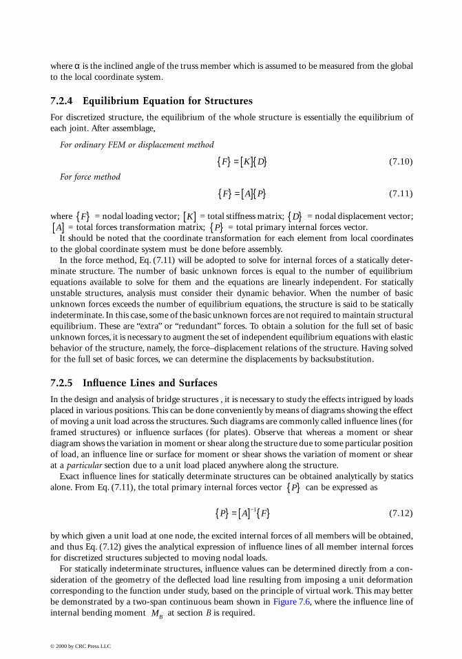
In the design and analysis of bridge structures , it is necessary to study the effects intrigued by loadsplaced in various positions. This can be done conveniently by means of diagrams showing the effectof moving a unit load across the structures. Such diagrams are commonly called influence lines (forframed structures) or influence surfaces (for plates). Observe that whereas a moment or sheardiagram shows the variation in moment or shear along the structure due to some particular positionof load, an influence line or surface for moment or shear shows the variation of moment or shearat a particular section due to a unit load placed anywhere along the structure.
Exact influence lines for statically determinate structures can be obtained analytically by staticsalone. From Eq. (7.11), the total primary internal forces vector can be expressed as
(7.12)
by which given a unit load at one node, the excited internal forces of all members will be obtained,and thus Eq. (7.12) gives the analytical expression of influence lines of all member internal forcesfor discretized structures subjected to moving nodal loads.
For statically indeterminate structures, influence values can be determined directly from a con-sideration of the geometry of the deflected load line resulting from imposing a unit deformationcorresponding to the function under study, based on the principle of virtual work. This may betterbe demonstrated by a two-span continuous beam shown in Figure 7.6, where the influence line ofinternal bending moment at section B is required.
F K D{ } = [ ]{ }
F A P{ } = [ ]{ }
F{ } K[ ] D{ }A[ ] P{ }
P{ }
P A F{ } = [ ] { }−1
MB
© 2000 by CRC Press LLC
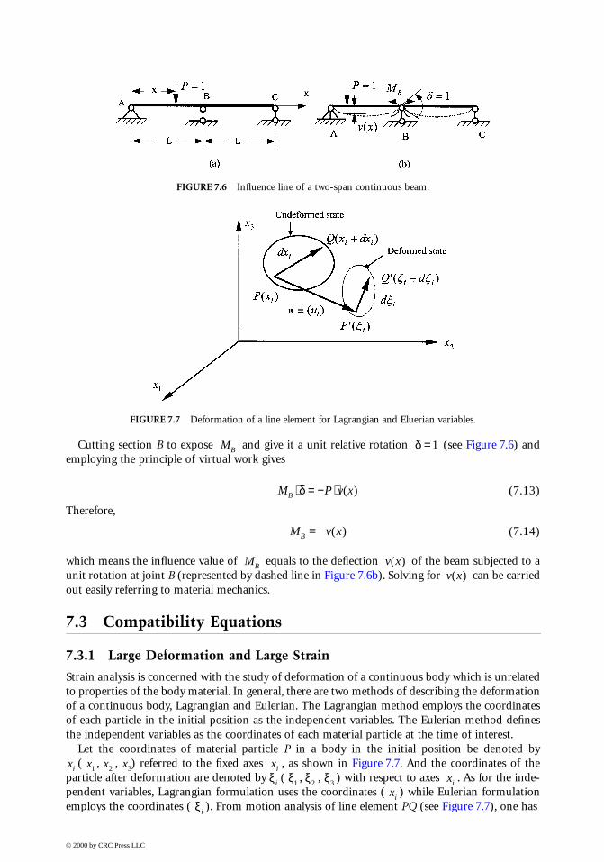
Cutting section B to expose and give it a unit relative rotation (see Figure 7.6) andemploying the principle of virtual work gives
(7.13)
Therefore,
(7.14)
which means the influence value of equals to the deflection of the beam subjected to aunit rotation at joint B (represented by dashed line in Figure 7.6b). Solving for can be carriedout easily referring to material mechanics.
7.3 Compatibility Equations
7.3.1 Large Deformation and Large Strain
Strain analysis is concerned with the study of deformation of a continuous body which is unrelatedto properties of the body material. In general, there are two methods of describing the deformationof a continuous body, Lagrangian and Eulerian. The Lagrangian method employs the coordinatesof each particle in the initial position as the independent variables. The Eulerian method definesthe independent variables as the coordinates of each material particle at the time of interest.
Let the coordinates of material particle P in a body in the initial position be denoted by( , , ) referred to the fixed axes , as shown in Figure 7.7. And the coordinates of the
particle after deformation are denoted by ( , , ) with respect to axes . As for the inde-pendent variables, Lagrangian formulation uses the coordinates ( ) while Eulerian formulationemploys the coordinates ( ). From motion analysis of line element PQ (see Figure 7.7), one has
FIGURE 7.6 Influence line of a two-span continuous beam.
FIGURE 7.7 Deformation of a line element for Lagrangian and Eluerian variables.
MB δ =1
M P v xB ⋅ = − ⋅δ ( )
M v xB = − ( )
MB v x( )v x( )
xi x1 x2 x3 xi
ξ i ξ1 ξ2 ξ3 xi
xi
ξ i
© 2000 by CRC Press LLC
For Lagrangian formulation, the Lagrangian strain tensor is
(7.15)
where and all quantities are expressed in terms of ( ).
For Eulerian formulation, the Eulerian strain tensor is
(7.16)
where and all quantities are described in terms of ( ).If the displacement derivatives and are not so small that their nonlinear terms cannot
be neglected, it is called large deformation, and the solving of will be rather difficult since thenonlinear terms appear in the governing equations.
If both the displacements and their derivatives are small, it is immaterial whether the derivativesin Eqs. (7.15) and (7.16) are calculated using the ( ) or the ( ) variables. In this case bothLagrangian and Eulerian descriptions yield the same strain–displacement relationship:
(7.17)
which means small deformation, the most common in structural engineering.For given displacements ( ) in strain analysis, the strain components ( ) can be determined
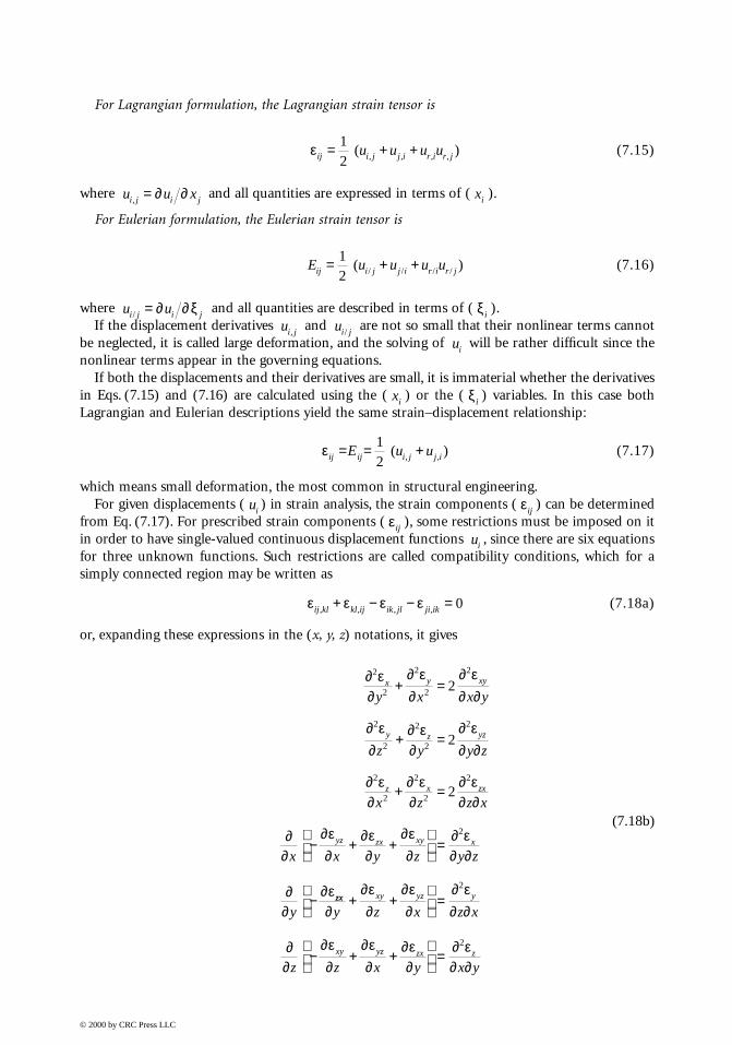
from Eq. (7.17). For prescribed strain components ( ), some restrictions must be imposed on itin order to have single-valued continuous displacement functions , since there are six equationsfor three unknown functions. Such restrictions are called compatibility conditions, which for asimply connected region may be written as
(7.18a)
or, expanding these expressions in the (x, y, z) notations, it gives
(7.18b)
εij i j j i r i r ju u u u= + +12
( ), , , ,
u u xi j i j, = ∂ ∂ xi
E u u u uij i j j i r i r j= + +12
( )/ / / /
u ui j i j/ = ∂ ∂ξ ξ i
ui j, ui j/
ui
xi ξ i
εij ij i j j iE u u= = +12
( ), ,
ui εij
εij
ui
ε ε ε εij kl kl ij ik jl ji ik, , , ,+ − − =0
∂ ε∂
∂ ε∂
∂ ε∂ ∂
∂ ε∂
∂ ε∂
∂ ε∂ ∂
∂ ε∂
∂ ε∂
∂ ε∂ ∂
∂∂
∂ε∂
∂ε∂
∂ε∂
∂ ε∂ ∂
∂∂
∂ε
2
2
2
2
2
2
2
2
2
2
2
2
2
2
2
2
2
2
2
x y xy
y z yz
z x zx
yz zx xy x
y x x y
z y y z
x z z x
x x y z y z
y
+ =
+ =
+ =
− + +
=
− zxzx xy yz y
xy yz zx z
y z x z x
z z x y x y
∂∂ε∂
∂ε∂
∂ ε∂ ∂
∂∂
∂ε∂
∂ε∂
∂ε∂
∂ ε∂ ∂
+ +
=
− + +
=
2
2
© 2000 by CRC Press LLC
Any set of strains and displacements , that satisfies Eqs. (7.17) and (7.18a) or (7.18b), aswell as displacement boundary conditions, is a kinematics admissible set, or a compatible set.
7.3.2 Compatibility Equation for Elements
For ordinary FEM, compatibility requirements are self-satisfied in the formulating procedure. Asfor equilibrium equations, a basic set of independent displacements can be identified for eachmember, and the kinematics relationships between member basic displacements and member–enddisplacements of one member can be given as follows:
(7.19)
where is element primary displacement vector, and have been shown inSection 7.2.2. For plane truss member, = , where ∆ is the relative displacement of themember (see Figure 7.5). It should also be noted that the physical basis of Eq. (7.19) is the overallcompatibility of the element.
7.3.3 Compatibility Equation for Structures
For the whole structure, one has the following equation after assembly process:
(7.20)
where = total primary displacement vector; = total nodal displacement vector; and = the transposition of described in Section 7.2.4.
A statically determinate structure is kinematically determinate. Given a set of basic memberdisplacements, there are a sufficient number of compatibility relationships available to allow thestructure nodal displacements to be determined. In addition to their application to settlement andfabrication error loading, thermal loads can also be considered for statically determinate structures.External forces on a structure cause member distortions and, hence, nodal displacements, but beforesuch problems can be solved, the relationships between member forces and member distortionsmust be developed. These will be shown in Section 7.5.1.
7.3.4 Contragredient Law
During the development of the equilibrium and compatibility relationships, it has been noticed thatvarious corresponding force and displacement transformations are the transposition of each other, asshown not only in Eqs. (7.5) and (7.19) of element equilibrium and compatibility relations, but also inEqs. (7.11) and (7.20) of global equilibrium and compatibility relations, although each pair of thesetransformations was obtained independently of the other in the development. These special sets ofrelations are termed the contragredient law which was established on the basis of virtual work concepts.Therefore, after a particular force transformation matrix is obtained, the corresponding displacementtransformation matrix would be immediately apparent, and it remains valid to the contrary.
7.4 Constitutive Equations
7.4.1 Elasticity and Plasticity
A material body will produce deformation when subjected to external excitations. If upon the releaseof applied actions the body recovers its original shape and size, it is called an elastic material, or
εij ui
∆{ } = [ ] { }e T eL d
∆{ } e L[ ] de{ }
∆{ } e ∆{ }
∆{ } = [ ] { }A DT
∆{ } D{ }A T[ ] A[ ]
© 2000 by CRC Press LLC
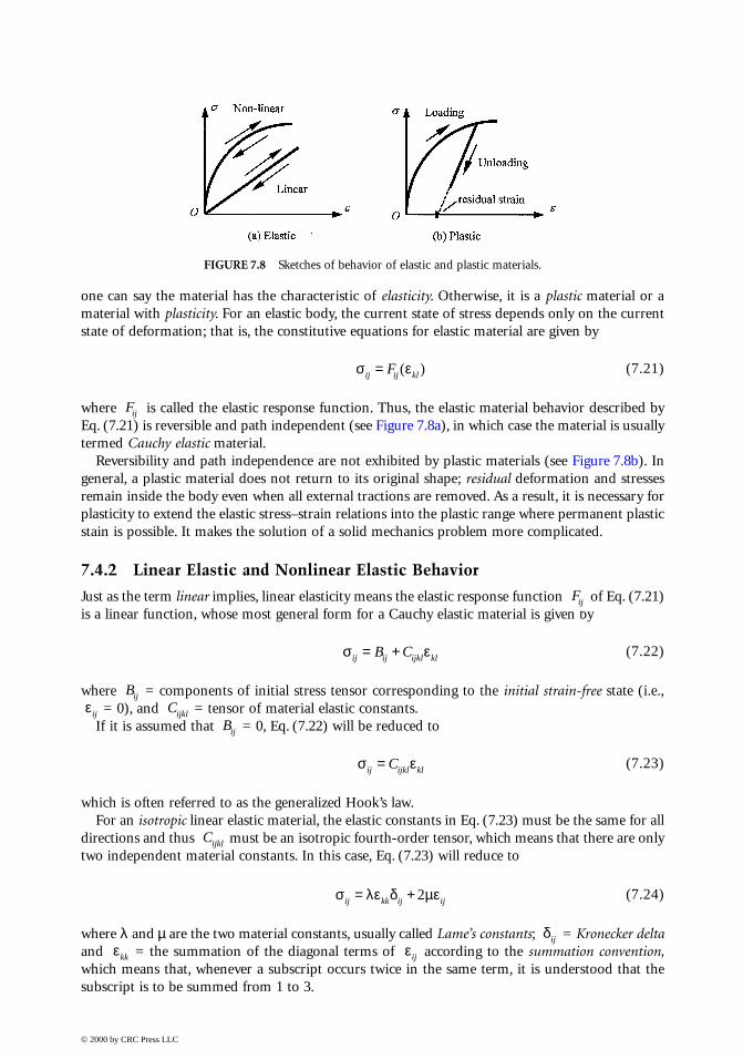
one can say the material has the characteristic of elasticity. Otherwise, it is a plastic material or amaterial with plasticity. For an elastic body, the current state of stress depends only on the currentstate of deformation; that is, the constitutive equations for elastic material are given by
(7.21)
where is called the elastic response function. Thus, the elastic material behavior described byEq. (7.21) is reversible and path independent (see Figure 7.8a), in which case the material is usuallytermed Cauchy elastic material.
Reversibility and path independence are not exhibited by plastic materials (see Figure 7.8b). Ingeneral, a plastic material does not return to its original shape; residual deformation and stressesremain inside the body even when all external tractions are removed. As a result, it is necessary forplasticity to extend the elastic stress–strain relations into the plastic range where permanent plasticstain is possible. It makes the solution of a solid mechanics problem more complicated.
7.4.2 Linear Elastic and Nonlinear Elastic Behavior
Just as the term linear implies, linear elasticity means the elastic response function of Eq. (7.21)is a linear function, whose most general form for a Cauchy elastic material is given by
(7.22)
where = components of initial stress tensor corresponding to the initial strain-free state (i.e., = 0), and = tensor of material elastic constants.
If it is assumed that = 0, Eq. (7.22) will be reduced to
(7.23)
which is often referred to as the generalized Hook’s law.For an isotropic linear elastic material, the elastic constants in Eq. (7.23) must be the same for all
directions and thus must be an isotropic fourth-order tensor, which means that there are onlytwo independent material constants. In this case, Eq. (7.23) will reduce to
(7.24)
where λ and µ are the two material constants, usually called Lame’s constants; = Kronecker deltaand = the summation of the diagonal terms of according to the summation convention,which means that, whenever a subscript occurs twice in the same term, it is understood that thesubscript is to be summed from 1 to 3.
FIGURE 7.8 Sketches of behavior of elastic and plastic materials.
σ εij ij klF= ( )
Fij
Fij
σ εij ij ijkl klB C= +
Bij
εij Cijkl
Bij
σ εij ijkl klC=
Cijkl
σ λε δ µεij kk ij ij= +2
δij
εkk εij
© 2000 by CRC Press LLC
If the elastic response function in Eq. (7.21) is not linear, it is called nonlinear elastic, andthe material exhibits nonlinear mechanical behavior even when sustaining small deformation. Thatis, the material elastic “constants” do not remain constant any more, whereas the deformation canstill be reversed completely.
7.4.3 Geometric Nonlinearity
Based on the sources from which it arises, nonlinearity can be categorized into material nonlinearity(including nonlinear elasticity and plasticity) and geometric nonlinearity. When the nonlinear termsin the strain–displacement relations cannot be neglected (see Section 7.3.1) or the deflections arelarge enough to cause significant changes in the structural geometry, it is termed geometric non-linearity. It is also called large deformation, and the principle of superposition derived from smalldeformations is no longer valid. It should be noted that for accumulated large displacements withsmall deformations, it could be linearized by a step-by-step procedure.
According to the different choice of reference frame, there are two types of Lagrangian formulation:the total Lagrangian formulation, which takes the original unstrained configuration as the referenceframe, and the updated Lagrangian formulation based on the latest-obtained configuration, which areusually carried out step by step. Whatever formulation one chooses, a geometric stiffness matrix orinitial stress matrix will be introduced into the equations of equilibrium to take account of the effectsof the initial stresses on the stiffness of the structure. These depend on the magnitude or conditions ofloading and deformations, and thus cause the geometric nonlinearity. In beam–column theory, this iswell known as the second-order or the P–∆ effect. For detailed discussions, see Chapter 36.
7.5 Displacement Method
7.5.1 Stiffness matrix for elements
In displacement method, displacement components are taken as primary unknowns. FromEqs. (7.5) and (7.19) the equilibrium and compatibility requirements on elements have beenacquired. For a statically determinate structure, no subsidiary conditions are needed to obtaininternal forces under nodal loading or the displaced position of the structure given the basicdistortion such as support settlement or fabrication errors. For a statically indeterminate structure,however, supplementary conditions, namely, the constitutive law of materials constructing thestructure, should be incorporated for the solution of internal forces as well as nodal displacements.
From structural mechanics, the basic stiffness relationships for a member between basic internalforces and basic member–end displacements can be expressed as
(7.25)
where is the element basic stiffness matrix, which can be termed for a conventionalplane truss member (see Figure 7.4).
Substitution of Eqs. (7.19) and (7.25) into Eq. (7.5) yields
(7.26)
where
(7.27)
Fij
P ke e e{ } = [ ] { }∆
k e[ ] EA l[ ]
F L k L d
k d
e e T e
e e
{ } = [ ][ ] [ ] { }= [ ] { }
k L k Le e T[ ] = [ ][ ] [ ]
© 2000 by CRC Press LLC
is called the element stiffness matrix, the same as in Eq. (7.4). It should be kept in mind that theelement stiffness matrix is symmetric and singular, since given the member–end forces,member–end displacements cannot be determined uniquely because the member may undergorigid body movement.
7.5.2 Stiffness Matrix for Structures
Our final aim is to obtain equations that define approximately the behavior of the whole body orstructure. Once the element stiffness relations of Eq. (7.26) is established for a generic element, theglobal equations can be constructed by an assembling process based on the law of compatibilityand equilibrium, which are generally expressed in matrix notation as
(7.28)
where is the stiffness matrix for the whole structure. It should be noted that the basic idea ofassembly involves a minimization of total potential energy, and the assembled stiffness matrix is symmetric and banded or sparsely populated.
Eq. (7.28) tells us the capabilities of a structure to withstand applied loading rather than the truebehavior of the structure if boundary conditions are not introduced. In other words, withoutboundary conditions, there can be an infinite number of possible solutions since stiffness matrix
is singular; that is, its determinant vanishes. Hence, Eqs. (7.28) should be modified to reflectboundary conditions and the final modified equations are expressed by inserting overbars as
(7.29)
7.5.3 Matrix Inversion
It has been shown that sets of simultaneous algebraic equations are generated in the application ofboth the displacement method and the force method in structural analysis, which are usually linear.The coefficients of the equations are constant and do not depend on the magnitude or conditionsof loading and deformations, since linear Hook’s law is generally assumed valid and small strainsand deformations are used in the formulation. Solving Eq. (7.29) is, namely, to invert the modifiedstiffness matrix . This requires tremendous computational efforts for large-scale problems. Theequations can be solved by using direct, iterative, or other methods. Two steps of elimination andbacksubstitution are involved in the direct procedures, among which are Gaussian elimination anda number of its modifications. These are some of the most widely used sets of direct methodsbecause of their better accuracy and small number of arithmetic operations.
7.5.4 Special Consideration
In practice, a variety of special circumstances, ranging from loading to internal member conditionsand supporting conditions, should be given due consideration in structural analysis.
Initially strains, which are not directly associated with stresses, result from two causes, thermalloading or fabrication error. If the member with initial strains is unconstrained, there will be a setof initial member–end displacements associated with these initial strains, but nevertheless no initialmember–end forces. For a member constrained to act as part of a structure, the general memberforce–displacement relationships will be modified as follows:
(7.30a)
ke[ ]
F K D{ } = [ ]{ }
K[ ]K[ ]
K[ ]
F K D{ } = [ ]{ }
K[ ]
F k d de e e e{ } = [ ] { } − { }( )0
© 2000 by CRC Press LLC
or
(7.30b)
where
(7.31)
are fixed-end forces, and a vector of initial member–end displacements for the member.It is interesting to note that a support settlement may be regarded as an initial strain. Moreover,
initial strains including thermal loading and fabrication errors, as well as support settlements, canall be treated as external excitations. Hence, the corresponding fixed-end forces as well as theequivalent nodal loading can be obtained which makes the conventional procedure describedpreviously still practicable.
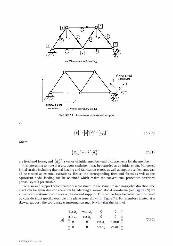
For a skewed support which provides a constraint to the structure in a nonglobal direction, theeffect can be given due consideration by adapting a skewed global coordinate (see Figure 7.9) byintroducing a skewed coordinate at the skewed support. This can perhaps be better demonstratedby considering a specific example of a plane truss shown in Figure 7.9. For members jointed at askewed support, the coordinate transformation matrix will takes the form of
(7.32)
FIGURE 7.9 Plane truss with skewed support.
F k d Re e e
F
e{ } = [ ] { } + { }0
R k dF
e e e
0 0{ } = −[ ] { }d
e
0{ }
α
α αα α
α αα α
[ ] =
−
−
cos sin
sin cos
cos sin
sin cos
i i
i i
j j
j j
0 0
0 0
0 0
0 0
© 2000 by CRC Press LLC
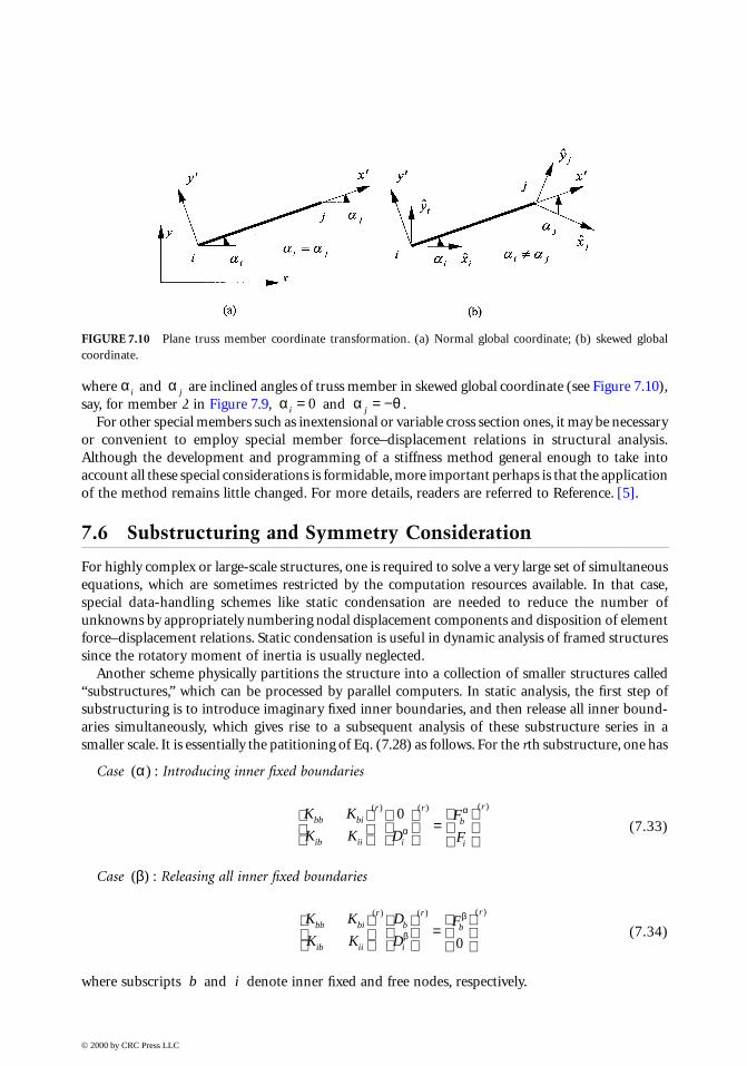
where and are inclined angles of truss member in skewed global coordinate (see Figure 7.10),say, for member 2 in Figure 7.9, and .
For other special members such as inextensional or variable cross section ones, it may be necessaryor convenient to employ special member force–displacement relations in structural analysis.Although the development and programming of a stiffness method general enough to take intoaccount all these special considerations is formidable, more important perhaps is that the applicationof the method remains little changed. For more details, readers are referred to Reference. [5].
7.6 Substructuring and Symmetry Consideration
For highly complex or large-scale structures, one is required to solve a very large set of simultaneousequations, which are sometimes restricted by the computation resources available. In that case,special data-handling schemes like static condensation are needed to reduce the number ofunknowns by appropriately numbering nodal displacement components and disposition of elementforce–displacement relations. Static condensation is useful in dynamic analysis of framed structuressince the rotatory moment of inertia is usually neglected.
Another scheme physically partitions the structure into a collection of smaller structures called“substructures,” which can be processed by parallel computers. In static analysis, the first step ofsubstructuring is to introduce imaginary fixed inner boundaries, and then release all inner bound-aries simultaneously, which gives rise to a subsequent analysis of these substructure series in asmaller scale. It is essentially the patitioning of Eq. (7.28) as follows. For the rth substructure, one has
Case : Introducing inner fixed boundaries
(7.33)
Case : Releasing all inner fixed boundaries
(7.34)
where subscripts and denote inner fixed and free nodes, respectively.
FIGURE 7.10 Plane truss member coordinate transformation. (a) Normal global coordinate; (b) skewed globalcoordinate.
α i α j
α i = 0 α θj = −
( )α
K K
K K D
F
Fbb bi
ib ii
r
i
r
b
i
r
=
( ) ( ) ( )0
α
α
( )β
K K
K K
D
DFbb bi
ib ii
rb
i
r
b
r
=
( ) ( ) ( )
β
β
0
b i
© 2000 by CRC Press LLC
Combining Eqs. (7.33) and (7.34) gives the force–displacement relations for enlarged elements substructures which may be expressed as
(7.35)
which is analogous to Eq. (7.26) and . And thereby the con-ventional procedure is still valid.
Similarly, in the cases of structural symmetry of geometry and material, proper consideration ofloading symmetry and antisymmetry can give rise to a much smaller set of governing equations.
For more details, please refer to the literature on structural analysis.
References
1. Chen, W.F. and Saleeb, A.F., Constitutive Eqs. for Engineering Materials, Vols. 1 & 2, Elsevier ScienceLtd., New York, 1994.
2. Chen, W.F., Plasticity in Reinforced Concrete, McGraw-Hill, New York, 1982.3. Chen, W.F. and T. Atsuta, Theor y of Beam-C olumns, Vol. 1, In-Plane Behavior and Design, McGraw-
Hill, New York, 1976.4. Desai, C.S., Ele mentary Finite Ele ment Method, Prentice-Hall, Englewood Cliffs, NJ, 1979.5. Meyers, V.J., Matrix Analysis of Structures, Harper & Row, New York, 1983.6. Michalos, J., Theor y of Structural Analysis and Design, Ronald Press, New York, 1958.7. Hjelmstad, K.D., Fundamentals of Structural Mechanics, Prentice-Hall College Div., Upper Saddle
River, NJ, 1996.8. Fleming, J.F., Analysis of Structural Systems, Prentice-Hall College Div., Upper Saddle River, NJ,
1996.9. Dadeppo, D.A. Introduction to Structural Mechanics and Analysis, Prentice-Hall College Div.,
Upper Saddle River, NJ, 1998.
K D Fb
r
b
r
b
r[ ] { } = { }( ) ( ) ( )
F F K K Fb
r
br
bir
iir
ir{ } = { } −[ ][ ] { }−( ) ( ) ( ) ( ) ( )1
© 2000 by CRC Press LLC