Duan, M., Perdikaris, P.C., Chen, W. Impact Effect of ...freeit.free.fr/Bridge Engineering HandBook/ch56.pdf · The bridge is designed to carry a speciﬁed truck of HS20-44. Solution

Duan, M., Perdikaris, P.C., Chen, W. "Impact Effect of Moving Vehicles." Bridge Engineering Handbook. Ed. Wai-Fah Chen and Lian Duan Boca Raton: CRC Press, 2000

56Impact Effect of

Moving Vehicles

56.1 Introduction

56.2 Consideration of Impact Effect in Highway Bridge Design

56.3 Consideration of Impact Effect in Railway Bridge Design

56.4 Free Vibration AnalysisStructural Models • Free Vibration Analysis

56.5 Forced Vibration Analysis under

Moving LoadDynamic Response Analysis • Summary of Bridge Impact Behavior

56.1 Introduction

Vehicles such as trucks and trains passing bridges at certain speeds will cause dynamic effects, amongthem global vibration and local hammer effects. The dynamic loads for moving vehicles are con-sidered “impact” in bridge engineering because of the relatively short duration. The magnitude ofthe dynamic response depends on the bridge span, stiffness and surface roughness, and vehicledynamic characteristics such as moving speed and isolation system. Unlike earthquake loads whichcan cause vibration in bridge longitudinal, transverse, and vertical directions, moving vehiclesmainly excite vertical vibration of the bridge. Impact effect has influence primarily on the super-structure and some of substructure members above the ground because the energy will be dissipatedeffectively in members underground by the bearing soils.

Although the interaction between moving vehicles and bridges is rather complex, the dynamiceffects of moving vehicles on bridges are accounted for by a dynamic load allowance, IM, in additionto static live load (LL) in the current bridge design specifications [1–3]. According to the AmericanAssociation of State Highway and Transportation Officials (AASHTO) and the American RailwayEngineering Association (AREA) specifications,

(56.1)

where Ddyn is the maximum dynamic response for deflection, moment, or shear of the structuralmembers and Dst is the corresponding maximum static response. The total live-load effect, LL, canthen be expressed as

LL = AF Dst (56.2)

IMD

D = 1dyn

st

−

×

Mingzhu DuanQuincy Engineering, Inc.

Philip C. PerdikarisCase Western Reserve University

Wai-Fah ChenPurdue University

© 2000 by CRC Press LLC

and

AF = 1 + IM (56.3)

where AF is the amplification factor representing the dynamic amplification of the static load effectand IM is the impact factor determined by an empirical formula in design code. No dynamic analysisis thus required in the design practice.

Most early research work on the dynamic bridge behavior of bridges under moving vehiclesfocused on an analytical approach modeling a bridge as a simply supported beam [5] or a simplysupported plate [8] under constant or pulsating moving loads (moving load model). The dynamiceffects under different speeds of the moving loads and different damping ratios were studied. It wasfound that the speed of vehicles and the fundamental period of the bridge dominate the dynamicbehavior of the bridge. Since most bridges consist of both beams and plates such as girder deckbridges, the above simplified model has limited validity. Along with analytical study, numericalmethods such as finite-element analysis and the finite-difference method have been used recentlyin studying the dynamic response of a vehicle–bridge system [10,21]. Two sets of equations ofmotion were developed for the bridge and vehicle, respectively. These equations are coupled at thecontacting points between bridge and vehicle and the contact points are time and space dependentdue to vehicles moving along a rough surface. An iteration procedure should be used to solve thecoupled equations. Field measurements are another alternative to investigate the dynamic effect[13] which disclosed the range of live-load effect for steel I-girder bridges under truck load.

Based on analytical analysis and field measurement studies, major characteristics of the bridgedynamic response under moving vehicles can be summarized as follows:

1. Measured impact factors [13], IM, on highway bridges vary significantly, e.g., with the meanof about 0.12 and the standard deviation of about 0.05 for steel I-girder bridges. The measuredimpact factors are well below those of the AASHTO specifications.

2. Impact factor increases as vehicle speed increases in most cases.3. Impact factor decreases as bridge span increases.4. Under the conditions of “very good” road surface roughness (amplitude of highway profile

curve is less than 1 cm), the impact factor is well below that in design specifications. But theimpact factor increases tremendously with increasing road surface roughness from “good”to “poor” (the amplitude of highway profile curve is more than 4 cm) and can be well beyondthe impact factor in design specifications.

5. Impact factor decreases as vehicles travel in more than one lane. The chance of maximumdynamic response occurring at the same time for all vehicles is small.

6. Impact factor for exterior girders is much larger than for interior girders because the excitedtorsion mode shapes contribute to the dynamic response of exterior girders.

7. The first mode shape of the bridge is dominant in most cases, especially for the dynamiceffect in the interior girder in single-span bridges.

The impact factor, IM, is a well-accepted measurement for the dynamic effect of bridges undermoving vehicles and is used in design specifications worldwide. Consideration of impact effect forhighway and railway bridges in design practice will be introduced through examples in Sections 56.2and 56.3, respectively. Free vibration and forced vibration by a moving vehicle will be introducedin Sections 56.4 and 56.5 to disclose the dynamic behavior of the bridge vibration.

56.2 Consideration of Impact Effect in Highway Bridge Design

Since the impact effect on bridges by moving vehicles is influenced by factors such as bridge span,stiffness, surface roughness, and speed and suspension system of moving vehicles, the impact factor


varies within a large range. While the actual modeling of this effect is complex, the calculation ofimpact effect is greatly simplified in the bridge design practice by avoiding any analysis of vehicle-induced vibration. In general, the dynamic effect is contributed by two sources: (1) local hammereffect by the vehicle wheel assembly riding surface discontinuities such as deck joints, cracks,delaminations, and potholes; and (2) global vibration caused by vehicles moving on long undula-tions in the roadway pavement, such as those caused by settlement of fill, or by resonant excitationof the bridge. The first source has a local impact effect on bridge joints and expansions. On theother hand, the second source will have influence on most of the superstructure members and someof the substructure members. A variety of considerations and design formulas are proposed world-wide for the second source, which means that the bridge community has not reached a consensuson this issue [4]. The differences among various code specifications worldwide for the dynamicamplification factor vs. the fundamental frequency are large. A large dynamic effect is consideredin some countries for the bridge frequency ranging from 1.0 to 5.0 Hz, which is the frequency rangeof the fundamental frequencies of most truck suspension systems. It is largely an attempt to penalizethe bridge designed within this frequency range. But the accurate evaluation of the first frequencyof a bridge can be hardly performed in the design stage.

In the AASHTO Standard Specifications of Highway Bridges (1996) in the United States, the impactfactor due to bridge vibration for members in Group A including superstructure, piers, and thoseportions of concrete and steel piles above the ground that support the superstructure, is simplyexpressed as a function of bridge span:

(56.4)

where L (in ft) is the length of span loaded to create maximum stress.In the AASHTO LRFD Bridge Design Specifications (1994), the static effects of the design truck

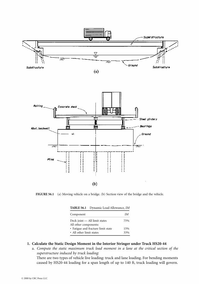
or tandem shall be increased by the impact effect in the percentage specified in Table 56.1.In Table 56.1, 75% of the impact effect is considered for deck joints for all limit states due to

local hammer effect, 15% for fatigue and fracture limit states for members vulnerable to cyclicloading such as shear connectors and welding members, and 33% for all other members influencedby global vibration. Field tests indicate that in the majority of highway bridges, the dynamiccomponent of the response does not exceed 25% of the static response to vehicles. Since the specifiedlive-load combination of the design truck and lane load represents a group of exclusion vehicleswhich are at least ⁴⁄₃ of those caused by the design truck alone on short- and medium-span bridges,the specified value of 33% in Table 56.1 is the product of ⁴⁄₃ and the basic 25%. The impact effectis not considered for retaining walls not subjected to vertical reactions from superstructure, andfor underground foundation components due to the damping effect of soil.

The dynamic effect caused by vehicles is accounted for in bridge design practice in the live-loadcalculation, as shown in the following example.

Example 56.1 — Live-Load Calculation in Highway Bridge DesignGivenThe bridge shown in Figure 56.2 is a steel girder-concrete deck bridge with a span of 50 ft (15.24 m).The bridge carrying two lanes of traffic loads consists of four girders with girder-to-girder spacingof 7 ft (2.13 m). The steel girders are W36 × 150 and the average concrete deck thickness is 9 in.(3.54 m). The bridge is designed to carry a specified truck of HS20-44.

Solution 1Using AASHTO Standard Specifications of Highway Bridges (1996) to calculate the design live-loadmoment for the interior steel girder under design truck HS20-44.

IML

=+

≤50125

0.30


1. Calculate the Static Design Moment in the Interior Stringer under Truck HS20-44 a. Compute the static maximum truck load moment in a lane at the critical section of the

superstructure induced by truck loading:There are two types of vehicle live loading: truck and lane loading. For bending momentscaused by HS20-44 loading for a span length of up to 140 ft, truck loading will govern.

FIGURE 56.1 (a) Moving vehicle on a bridge. (b) Section view of the bridge and the vehicle.

TABLE 56.1 Dynamic Load Allowance, IM

Component IM

Deck joint — All limit states 75%All other components:• Fatigue and fracture limit state 15%• All other limit states 33%


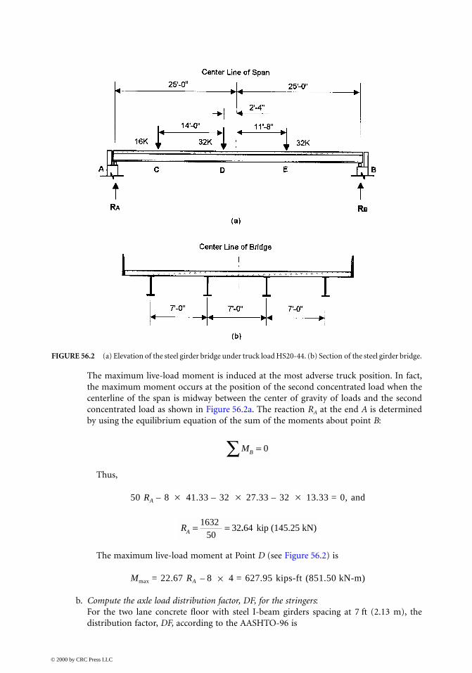
The maximum live-load moment is induced at the most adverse truck position. In fact,the maximum moment occurs at the position of the second concentrated load when thecenterline of the span is midway between the center of gravity of loads and the secondconcentrated load as shown in Figure 56.2a. The reaction RA at the end A is determinedby using the equilibrium equation of the sum of the moments about point B:

Thus,

50 RA – 8 41.33 – 32 27.33 – 32 13.33 = 0, and

The maximum live-load moment at Point D (see Figure 56.2) is

Mmax = 22.67 RA – 8 4 = 627.95 kips-ft (851.50 kN-m)

b. Compute the axle load distribution factor, DF, for the stringers:For the two lane concrete floor with steel I-beam girders spacing at 7 ft (2.13 m), thedistribution factor, DF, according to the AASHTO-96 is

FIGURE 56.2 (a) Elevation of the steel girder bridge under truck load HS20-44. (b) Section of the steel girder bridge.

MB =∑ 0

× × ×

RA = =1632 50

32 64 kip (145.25 kN).

×


c. Calculate the design static bending moment in a stringer:

MLL = DF(Mmax) = 627.95 0.64 = 401.89 kips-ft (544.96 kN-m)

2. Determine Dynamic Amplification Factor, AF

AF = (AASHTO-96)

3. Calculate the Total Bending Moment under Live Load The total live bending moment including the amplification factor is

MLL+IM = MLL AF

= 401.89 1.29 = 518.44 kips-ft (703.00 kN-m) (AASHTO-96)

Solution 2Using AASHTO-LRFD Design Specifications (1994) to calculate the design live-load moment for aninterior steel girder under truck HS20-44.

1. Calculate the Static Truck Moment in the Interior Girder under Truck HS20-44 a. The maximum moment in a lane is the same as in Method 1:

Mmax = 627.95 kips-ft (851.50 kN-m)

b. Compute the moment load distribution factor, DF, for the steel girders:For the two-lane concrete floor with steel I-girders spacing at 7 ft (2.13 m), the distributionfactor, DF, is

(for preliminary design use)

c. Calculate the design static bending moment in a stringer:

MLL = DF(Mmax) = 627.95 0.63 = 395.64 kips-ft (538.07 kN-m)

2. Determine Dynamic Amplification Factor, AF

AF = (AASHTO-94)

3. Calculate the Total Bending Moment in an Interior Stringer under Truck Load The total bending moment under truck load including the amplification factor is

MLL+IM (truck) = MLL AF = 395.64 1.33 = 526.20 kips-ft (715.64 kN-m) (AASHTO-94)

DFS=

×=

×=

2 5.57

2 5.5 0.64

×

1.0 1.050

1251.0

5050 125

1.29+ = ++

= ++

=IML

×

DFS S

L

K

Lt Lg= +

= +

× =0.075

9.5 12.00.075

7.09.5

7.01.0 0.6

0.6 0.2

s3

0.1 0.6 0.2

3

×

1.0 1.0 1.33+ = + =IM 0 33.

×


4. The vehicular live-load moment is the combination of the design truck load with impactallowance and design lane load without impact allowance (0.64 kip/ft over 10.0 ft per lane,0.88 kN/m over 3.0 m):

MLL+IM (total) = 526.20 + 0.63 (0.64 50/2 22.67 – 1/2 0.64 22.672)

= 651.10 kips-ft (885.50 kN-m)

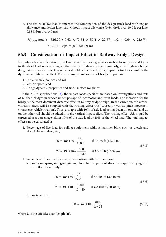
56.3 Consideration of Impact Effect in Railway Bridge Design

For railway bridges the ratio of live load caused by moving vehicles such as locomotive and trainsto the dead load is mostly higher than that in highway bridges. Similarly, as in highway bridgedesign, static live-load effect by vehicles should be increased by the impact factor to account for thedynamic amplification effect. The most important sources of bridge impact are

1. Initial vehicle bounce and roll,2. Vehicle speed, and3. Bridge dynamic properties and track-surface roughness.

In the AREA specifications [3], the impact loads specified are based on investigations and testsof railroad bridges in service under passage of locomotive and train loads. The vibration for thebridge is the most dominant dynamic effect in railway bridge design. In the vibration, the verticalvibration effect will be coupled with the rocking effect (RE) caused by vehicle pitch movement(transverse vehicle rotation). Thus, a couple with 10% of axle load acting down on one rail and upon the other rail should be added into the vertical impact effect. The rocking effect, RE, should beexpressed as a percentage; either 10% of the axle load or 20% of the wheel load. The total impacteffect can be calculated as

1. Percentage of live load for rolling equipment without hammer blow, such as diesels andelectric locomotives, etc.,

(56.5)

2. Percentage of live load for steam locomotives with hammer blow:a. For beam spans, stringers, girders, floor beams, parts of deck truss span carrying load

from floor beam only:

(56.6)

b. For truss spans:

(56.7)

where L is the effective span length (ft).

× × × × ×

IM RE L

L

IM REL

L

= + −

−−

≥

403

1600if < 50 ft (15.24 m)

= +16600

30if 80 ft (24.39 m)

2

IM REL

L

IM REL

L

= + −

−−

≥

40500

if < 100 ft (30.48 m)

= +101600

40if 0 ft (30.48 m)

2

10

IM REL

= + −104000

+ 25


Tests have shown that the impact load on ballasted deck bridges can be reduced to 90% of thatspecified for open-deck bridges because of the damping effect which results from a ballasted deckbridge. It was found from a parametric study [9] that the impact ranges from 24.9 to 26.0%, withan average of 25.6%, except for hangers. The following example shows how to account for impacteffect in live-load calculation in railway bridge design.

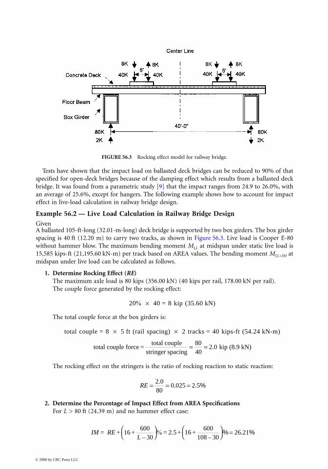
Example 56.2 — Live Load Calculation in Railway Bridge DesignGivenA ballasted 105-ft-long (32.01-m-long) deck bridge is supported by two box girders. The box girderspacing is 40 ft (12.20 m) to carry two tracks, as shown in Figure 56.3. Live load is Cooper E-80without hammer blow. The maximum bending moment MLL at midspan under static live load is15,585 kips-ft (21,195.60 kN-m) per track based on AREA values. The bending moment MLL+IM atmidspan under live load can be calculated as follows.

1. Determine Rocking Effect (RE) The maximum axle load is 80 kips (356.00 kN) (40 kips per rail, 178.00 kN per rail).The couple force generated by the rocking effect:

20% 40 = 8 kip (35.60 kN)

The total couple force at the box girders is:

total couple = 8 5 ft (rail spacing) 2 tracks = 40 kips-ft (54.24 kN-m)

The rocking effect on the stringers is the ratio of rocking reaction to static reaction:

2. Determine the Percentage of Impact Effect from AREA Specifications For L > 80 ft (24.39 m) and no hammer effect case:

FIGURE 56.3 Rocking effect model for railway bridge.

×

× ×

total couple force =total couple

stringer spacing2.0 kip (8.9 kN)= =80

40

RE = = =2.080

0.025 2.5%

IM REL

= + 16 +600– 30

% = 2.5 + 16 +600

108 – 3026.21%

=%


For ballasted deck bridges, 90% reduction should be considered, that is:

IM = 90% × 26.21% = 0.24

3. Determine Live-Load Effect of the Maximum Bending Moment at Midspan

AF = 1.0 + IM = 1.0 + 0.24 = 1.24

MLL+IM = AF (MLL ) = 1.24 15,585 = 19,264 kips-ft (26,199.04 kN-m)

56.4 Free Vibration Analysis

56.4.1 Structural Models

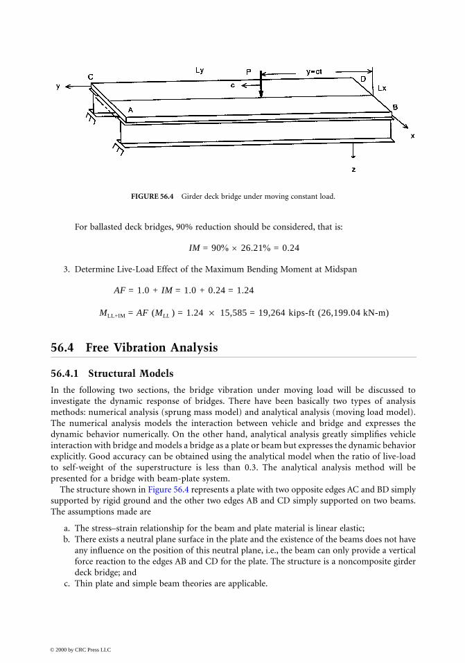
In the following two sections, the bridge vibration under moving load will be discussed toinvestigate the dynamic response of bridges. There have been basically two types of analysismethods: numerical analysis (sprung mass model) and analytical analysis (moving load model).The numerical analysis models the interaction between vehicle and bridge and expresses thedynamic behavior numerically. On the other hand, analytical analysis greatly simplifies vehicleinteraction with bridge and models a bridge as a plate or beam but expresses the dynamic behaviorexplicitly. Good accuracy can be obtained using the analytical model when the ratio of live-loadto self-weight of the superstructure is less than 0.3. The analytical analysis method will bepresented for a bridge with beam-plate system.

The structure shown in Figure 56.4 represents a plate with two opposite edges AC and BD simplysupported by rigid ground and the other two edges AB and CD simply supported on two beams.The assumptions made are

a. The stress–strain relationship for the beam and plate material is linear elastic;b. There exists a neutral plane surface in the plate and the existence of the beams does not have

any influence on the position of this neutral plane, i.e., the beam can only provide a verticalforce reaction to the edges AB and CD for the plate. The structure is a noncomposite girderdeck bridge; and

c. Thin plate and simple beam theories are applicable.

FIGURE 56.4 Girder deck bridge under moving constant load.

×


56.4.2 Free Vibration Analysis

The differential equation for free vibration of the plate shown in Figure 56.4 is

(56.8)

where

= the flexural rigidity of the plate

m = is the mass per unit area of the plateW = is the vertical deflection of the plate

The boundary conditions for the plate are as follows:

At y = 0 and y = Ly:

W (x, y, t) = 0 (56.9a)

My(x, y, t) = 0 (56.9b)

At x = 0:

Mx (x, y, t) = 0 (56.9c)

(56.9d)

At x = Lx:

Mx (x, y, t) = 0 (56.9e)

(56.9f)

where is the flexural rigidity and mass per unit beam length, respectively, and Mx,My are the transverse and longitudinal bending moments, respectively. Mxy is the torque and Qy isthe shear force at the edges of the plate, respectively. Their signs are shown in Figure 56.5. The termsat the right-hand side in Eqs. (56.9d) and (56.9f) represent the interaction forces at the edges ABand CD between the plate and the beams. It is seen that the participation of the beams is taken intoaccount in the partial differential equations through the boundary conditions for the plate.

Assuming that the structure vibrates in a mode so that the deflected shape is described by

(56.10)

the following equations can be derived by substituting Eq. (56.10) into Eq. (56.8):

(56.11)

D W m Wtt∇ + =( ) ( )4 2 0

DEh=

−

3

12(1 )µ

QM

yE I

Wy

mWtx

xyb b b+ = +

∂∂

∂∂

∂∂

4

4

2

2

QM

yE I

Wy

mWtx

xyb b b+ = − −

∂∂

∂∂

∂∂

4

4

2

2

E I mb b band

Wi yL

X x t qy

j ij= +sin sinπ ω( ) ( )

XiL

XiL

XmD

Xjy

jy

j ij j( ) ( )4

2 2

22

4 4

42 0− + − =π π ω


The solution to the homogeneous differential equation above is

Xj = eλ x/Lx

where λ must satisfy the characteristic equation:

(56.12)

There are four roots for this equation. According to the signs of the roots, Xj (x) will take twodifferent forms, which will be discussed separately.

Case 1

where

(56.13)

FIGURE 56.5 (a) A three-dimensional plate with length Ly and width Lx. (b) A volume element with inter forcesacting on its sides.

lL

iL

lL

iL

m

Dx y x y

ij44

2 2

2

2

2

4 4

4

2

2 0− + −

=π π ω

i prij2 2>

prmL

Dijij y22 2

4=ω

π


We have the following solution for Eq. (56.11)

(56.14)

where

u = x/L x (56.15.a)

(56.15.b)

By substituting Eq. (56.14) and (56.10) into the boundary conditions in Eqs. (56.9a) to (56.9f), theconstants A, B, and C in Eq. (56.14) can be determined by solving a group of eigenvalue equations [7].

The natural frequency in Case 1 can be obtained from the following nonlinear equationfrom the boundary conditions as

(56.16)

where

and Q in Eq. (56.16) represents the interaction between the plate and the beams.

Case 2

In this case, the solution for Eq. (56.11) would be

(56.17)

where

By substituting Eqs. (56.17) and (56.11) into the boundary conditions in Eqs. (56.9a) to (56.9f),we can obtain the constants in Eq. (56.17) as in Case 1 by solving a group of eigenvalue equations [7].

X u A u B u C u

i pr

j

ij

= + + +

= +[ ]sinh cosh sinh cosh

λ λ λ λ

λ πγ

1 1 2 2

1 22 2

,

γ = L Ly x/

ωij

2 1

2

0

1 2 12

22

1 2 12

14

22

24

1 2

1 22

1 2 1 2

2 22

1 2 1 12

1 2

2

λ λ λ λ λ λ λ λ

λ λ

λ λ λ λ λ λ

D D D D

D D Q Q D D

D D

( )

( )

cosh cosh sinh sinh

sinh sinh

sinh cosh cosh sinh

− − +( )

− +( ) + +

−( ) =

D i prij1 2

2

22 21, ( )= − +( )π

γµ

Q E DiL

m D Lb by

b ij y= −( ) /4 4

42 3π ω

i prij2 2<

X u A u B u C uj = + + +sin cos sinh coshλ λ λ λ1 1 2 2

l pr iij1 2

2 2, = [ ]π

γm


The natural frequency in Case 2 can be obtained from the following equation:

(56.18)

Example 56.3 Free Vibration Analysis for a Beam-Plate BridgeA one-lane bridge deck structure is shown in Figure 56.4. The plate is made of an isotropic materialrepresenting reinforced concrete, and the beams are made of steel with a W36 × 150 section. The bridgespan length is 80 ft (24.39 m) and the bridge width is 10 ft (3.05 m). The thickness of the deck plate is8 in. (3.15 cm). The elasticity modulus of the steel girder Eb = 29.0 103 ksi (200.0 103 MPa) andthe elasticity modulus of the concrete plate is E = 4.38 103 ksi (30.18 MPa). The mass density ofthe plate m = 0.8681 lb/in.2 g (0.61 kN/cm2 g) and the mass density of the beam is mb = 12.50 lb/in.2g(22.0 N/cm g) where g is the gravitational acceleration. The moment of inertia of the beam is

(375,800 cm4). All other properties are calculated as:

Bending rigidity of the plate in y direction:

Bending rigidity ratio between beam and plate:

Mass ratio between beam and plate:

First natural frequency of the plate as a beam:

First natural frequency of the beam:

Subscripts i and j represent the ith and jth mode shape in the y- and x-direction, respectively.The natural frequencies, , can be determined numerically using Eqs. (56.16) and (56.18). Someof the first several natural frequencies are shown in Table 56.2.

The mode shapes of the bridge are shown in Figures 56.6 and 56.7 using normalized dimensionsin all three directions. It is seen that W12, W14, W22, and W24 are all asymmetric mode shapes in the

ωij

2 1

2

0

1 2 12

22

1 2 12

14

22

24

1 2

1 22

1 2 1 2

2 22

1 2 1 12

1 2

2

λ λ λ λ λ λ λ λ

λ λ

λ λ λ λ λ λ

D D D D

D D Q Q D D

D D

( )

( )

cos cosh sin sinh

sin sinh

sin cosh cos sinh

− − +( )

− +( ) + +

−( ) =

× ××

Ib = 9030 4in.

L DL E t

xx=

− µ= × ×

310 2 12 2

12 1 04 56 10 1 28 10

( . ). lb.in. kN.cm( . )

Rej2.0EbIb

LxD------------------ 11.5= =

Rm

L mmb

x

= =

.0 12

ω11

2

2 4 40p

y

pL

Dm

= = . rad / s

ω1

2

2 30b

y

b b

b

pL

E I

m= = .45 rad / s

ωij


x-direction about the center line x = Lx/2. When a moving load traverses the plate along this line,these mode shapes would not be excited. Thus, there are no contributions from these mode shapes.

The first mode shape of the beam–plate system is nearly a constant in the x-direction, as shownin this example of a rather high plate aspect ratio. This means that the beams have the same firstmode shape as the plate. In this case, the first natural frequency of the beam–plate system can beapproximately evaluated as

(56.19)

where and are fundamental frequencies of the beam and plate as a beam, respectively.

TABLE 56.2 Natural Frequencies of One-Lane Bridge Deck (rad/s; plate aspect ratio = 8.0)

j = 1 j = 2 j = 3

i = 1 14.53 35.43 482.65i = 2 60.09 110.62 506.27i = 3 125.67 217.44 556.53i = 4 206.05 354.98 647.51

FIGURE 56.6 Normalized three-dimensional mode shapes Wij, i = 1, j = 1,2,3,4, for a one-lane bridge deck. (sub-scripts i-j is the mode shape number in y- and x-directions, respectively).

ω ω ω112 1

211

22

1 2= +

+R

Rm

b p

m

ω1b ω1

p


56.5 Forced Vibration Analysis under Moving Load

56.5.1 Dynamic Response Analysis

The governing equation for the plate with smooth surface supported by two beams under a movingconstant load shown in Figure 56.4 is

(0 < t < Ly/c) (56.20)

where

and c is the speed of the moving load, and P the magnitude of the moving load. A Dirac deltafunction represents a unit concentrated force acting on the deck.

FIGURE 56.7 Normalized three-dimensional mode shapes Wij, i = 2, j = 1,2,3,4, for a one-lane bridge deck (sub-scripts i-j is the mode shape number in y- and x-directions, respectively).

∇ + =42

2

1W

mD

Wt D

p x y t∂∂

( , , )

p x y t P y ct x Lx( , , ) ( ) ( / )= − −δ δ 2


The method of modal superposition is used to get the dynamic response by assuming

(56.21)

By substituting Eq. (56.21) into Eq. (56.20), the following ordinary differential equation can bederived:

(0 < t < Ly /c) (56.22)

where is the damping ratio for mode shape i–j. The initial condition is that the bridge structureis in a static state before the load enters the span and the structure is in a state of free vibrationafter the load traverses the bridge.

There are several parameters affecting the dynamic response of the structure. The influence ofsome typical parameters such as the speed of the moving load and damping ratio is presented inthe following.

The vehicle speed is normalized as

(56.23)

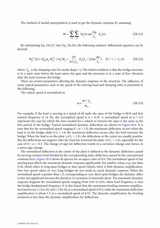
For example, if the load is moving at a speed of 60 mph, the span of the bridge is 80 ft and firstnatural frequency is 14 Hz, the normalized speed is α = 0.25. A normalized speed of α = 0.5represents the case for which the time needed for a vehicle to traverse the span is the same as thefirst period of the bridge. Typical normalized dynamic deflections are shown in Figure 56.8. It isseen that for the normalized speed ranging 0 < α < 1.0, the maximum deflection occurs when theload is on the bridge while if α > 1.0, the maximum deflection occurs after the load traverses thebridge. When the load is on the plate (ct/Ly < 1.0), the deflections at the center are usually positive.But the deflections are negative after the load has traversed the plate (ct/Ly > 1.0), especially for thecase of 0 < α < 0.5. The change of sign for deflection results in a curvature change and, hence, ina stress sign change.

The normalized deflection at the center of the plate is defined as the dynamic deflection causedby moving constant load divided by the corresponding static deflection caused by the concentratedconstant force. Figure 56.9 shows its spectra for an aspect ratio of 8.0. The normalized speed of themoving load affects the maximum dynamic response significantly. For small α values, e.g., less than0.20, which refers to long-span bridges or slow-speed vehicle, there is little dynamic amplification.Very low speed values or very long bridges do not result in much dynamic response. When thenormalized speed is greater than 1.3, corresponding to very short span bridges, the dynamic effectis also not significant because the duration of excitation is extremely short. The maximum dynamicresponse happens for normalized speeds ranging from 0.45 to 0.65, when load frequency is nearthe bridge fundamental frequency. It is also found that the maximum bending moment amplifica-tion factors are 1.2 for My and 1.1 for Mx at a normalized speed of 0.4, while the maximum deflectionamplification is about 1.5 at a normalized speed of 0.55. The dynamic amplification for bendingmoments is less than the dynamic amplification for deflections.

W W ti yL

X xijyji

j==

+∞

=

+∞

∑∑ ( ) ( )sinπ

11

W t W WP

m L LX L

i cL

tij t ij ij ij t ij ijx y

ij xy

,( )

,( )( ) ( / )2 1 22

22+ + =ξ ω ω π

sin

ξij

απ

ω=

c Ly/

11


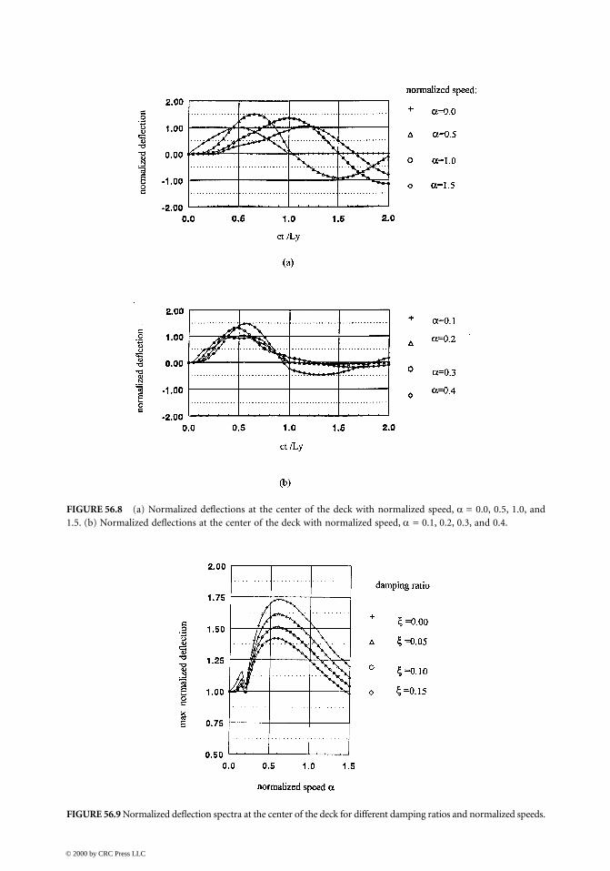
FIGURE 56.8 (a) Normalized deflections at the center of the deck with normalized speed, α = 0.0, 0.5, 1.0, and1.5. (b) Normalized deflections at the center of the deck with normalized speed, α = 0.1, 0.2, 0.3, and 0.4.

FIGURE 56.9 Normalized deflection spectra at the center of the deck for different damping ratios and normalized speeds.


56.5.2 Summary of Bridge Impact Behavior

For one-lane bridge deck structures, the conclusions of impact behavior of the bridge under movingconstant loads have been drawn as:

1. The maximum deflection occurs when the moving load traverses the deck at a normalizedspeed less than 1.0, and the maximum deflection occurs when the load passes the deck at anormalized speed larger than 1.0.

2. The maximum impact effect is mostly expected when the duration of moving vehicle is closeto the fundamental period of the bridge.

3. The aspect ratios of the deck play an important role. When they are less than 4.0, the firstmode shape is dominant, when more than 8.0, other mode shapes are excited. The contri-butions from higher natural frequency mode shapes decrease slowly due to the fact that thenatural frequency, ωij, increases slowly as subscript i increases. Thus, a sufficient number ofterms of superimposed mode shapes are needed to get more accurate results.

4. Dynamic amplification for deflections is larger than for bending moments. The responsecurves of deflections are “smoother” than the response curves for bending moments in thetime domain.

5. The dynamic response of a plate with two edges free and the other two edges simply supportedis close to a beam for aspect ratios of the plate larger than 2.0.

6. The analysis of a moving constant load model usually overestimates the dynamic effectbecause vehicle mass is not considered in the dynamic analysis and thus overestimates thefirst frequency of the bridge–vehicle system which corresponds to the “shorter-span” bridge.

Acknowledgments

The authors would like to express their gratitude to Prof. Dario Gasparini for his endeavors andopinions and to the financial support from Case Western Reserve University in performing thedynamic analysis. Mr. Kang Chen, MG Engineering, Inc. provided valuable information for therailway bridge part, which is greatly appreciated.

References

1. AASHTO, LRFD Bridge Design Specifications, American Association of State Highway and Trans-portation Officials, Washington, D.C., 1994.

2. AASHTO, Standard Specifications for Highway Bridges, 16th ed., American Association of StateHighway and Transportation Officials, Washington, D.C., 1996.

3. AREA, Manual for Railway Engineering, American Railway Engineering Association, Washington,D.C., 1996.

4. Barker, R. M. and Puckett, J. A., Design of Highway Bridges — Based on AASHTO LRFD, BridgeDesign Specifications, John Wiley & Sons, New York, 1996.

5. Biggs, J. M., Introduction to Structural Dynamics under Moving Loads, McGraw-Hill, New York,Inc., 1964.

6. Chang, D. and Lee, H., Impact factors for simple-span highway girder bridges, J. Struct. Eng. ASCE,120(3), 880–889, 1994.

7. Duan, M., Static Finite Element and Dynamic Analytical Study of Reinforced Concrete BridgeDecks, M.S. thesis, Department of Civil Engineering, Case Western Reserve University, Cleveland,OH, 1994.

8. Fryba, L., Introduction to Structural Dynamics, Groningen Noordhoff Futern, 1972.9. Garg, V. K., Dynamics of Railway Vehicle Systems, Harcourt Brace Jovanovich, New York, 1984.

10. Huang, D., Wang, T.-L., and Shahawy, M., Impact analysis of continuous multi-girder bridges dueto moving vehicles, J. Struct. Eng. ASCE, 118(12), 3427–3443, 1992.


11. Hino, J., Yoshimura, T., and Konishi, K., A finite element method prediction of the vibration of abridge subjected to a moving vehicle load, J. Sound Vibration, 96(6), 45–53, 1984.

12. Huang, D., Wang, T.-L., and Shahawy, M., Vibration of thin-walled box-girder bridges exited byvehicles, J. Struct. Eng. ASCE, 121(9), 1330–1337, 1995.

13. Kim, S. and Nowak, A., Load distribution and impact factors for I-girder bridges, J. Bridge Eng.ASCE, 2(3), 1997.

14. Lin, Y. H. and Trethewey, M. W., Finite element analysis of elastic beams subjected to moving loads,J. Sound Vibration, 136(2), 323–342, 1990.

15. Petrou, M. F., Perdikaris, P. C., and Duan, M., Static behavior of noncomposite concrete bridgedecks under concentrated loads, J. Bridge Eng. ASCE, 1(4), 143–154, 1996.

16. Scheling, D. R., Galdos, N. H., and Sahin, M. A., Evaluation of impact factors for horizontallycurved steel box bridges, J. Struct. Eng. ASCE, 118(11), 3203–3221, 1992.

17. Timoshenko, S. P. and Woinowsky-Krieger, S., Theory of Plates and Shells, 2nd ed., McGraw-Hill,New York, 1959.

18. Wang, T.-L., Huang, D., and Shahawy, M., Dynamic response of multi-girder bridges, J. Struct.Eng. ASCE, 118(8), 2222–2238, 1992.

19. Xanthakos, P., Theory and Design of Bridges, John Wiley & Sons, New York, 1994.20. Yang, Y.-B. and Lin, B.-H., Vehicle-bridge interaction analysis by dynamic condensation method,

J. Struct. Eng. ASCE, 121(2), 1636–1643, 1995.21. Yang, Y.-B. and Yau, J.-D., Vehicle-bridge interaction element for dynamic analysis, J. Struct. Eng.

ASCE, 118(11), 1512–1518, 1997.


Documents

Duan, M., Perdikaris, P.C., Chen, W. Impact Effect of ...freeit.free.fr/Bridge Engineering HandBook/ch56.pdf · The bridge is designed to carry a speciﬁed truck of HS20-44. Solution