LIS 570

Summarising and presenting data - Univariate analysis continued

Bivariate analysis

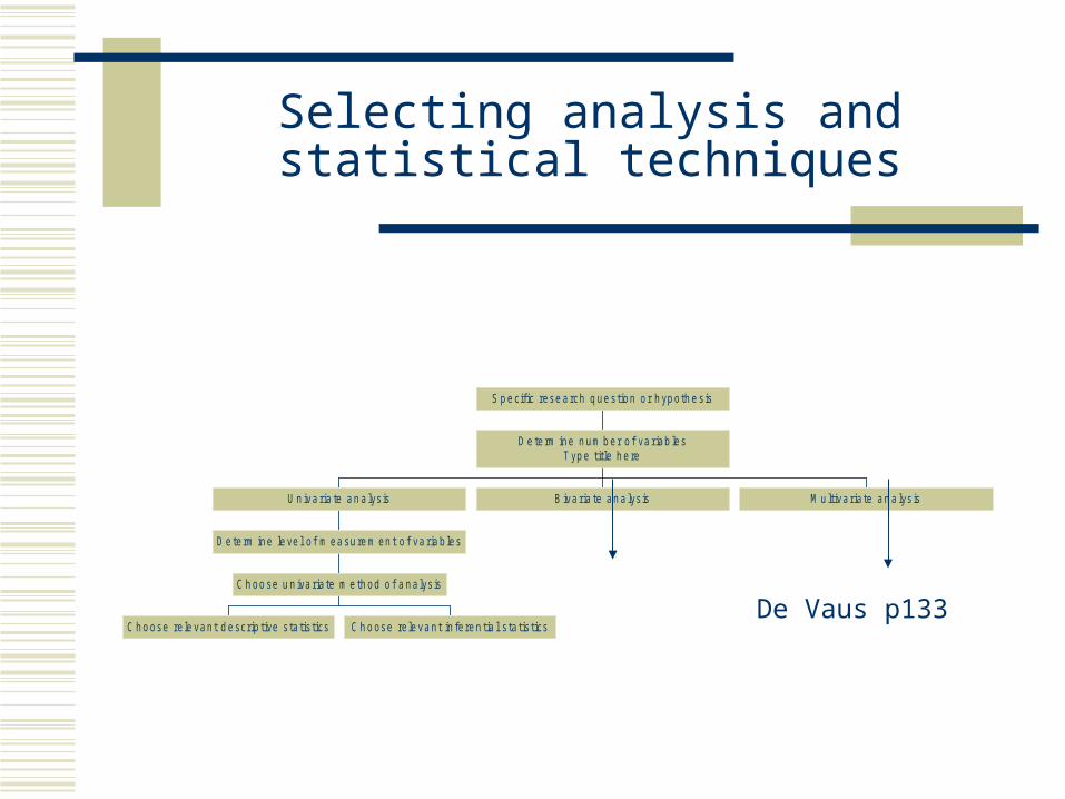
Selecting analysis and statistical techniques

C h o ose re le va n t d e sc rip tive s ta tis t ics C h o ose re le va n t in fe re n tia l s ta tis t ics

C h oo se u n iva ria te m e th od o f a n a lys is

D e te rm ine le ve l o f m ea su re m en t o f va ria b les

U n iva ria te a n a lys is B iva ria te a n a lys is M u lt iva ria te a n a lys is

D e te rm ine n um b er o f va riab lesT yp e t it le h e re

S p e cif ic rese a rch q ue s tion o r h yp o th e s is

De Vaus p133

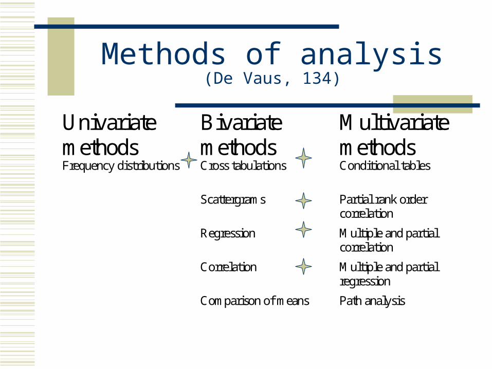
Methods of analysis (De Vaus, 134)

Univariatemethods

Bivariatemethods

Multivariatemethods

Frequency distributions Cross tabulations Conditional tables

Scattergrams Partial rank ordercorrelation

Regression Multiple and partialcorrelation

Correlation Multiple and partialregression

Comparison of means Path analysis

Summary

Inferential statistics for univariate analysis Bivariate analysis

crosstabulation the character of relationships - strength,

direction, nature correlation

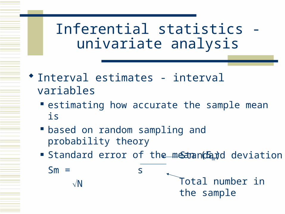
Inferential statistics - univariate analysis

Interval estimates - interval variables estimating how accurate the sample mean is based on random sampling and probability

theory Standard error of the mean (Sm)

Sm = s

N

Standard deviation

Total number in the sample

Standard Error

Probability theory for 95% of samples, the population mean will be

within + or - two standard error units of the sample mean

this range is called the confidence interval standard error is a function of sample size

to reduce the confidence interval, increase the sample size

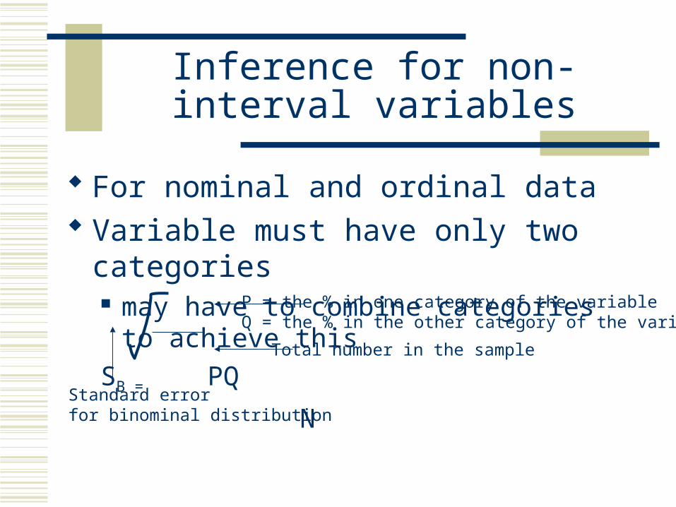
Inference for non-interval variables

For nominal and ordinal data Variable must have only two categories

may have to combine categories to achieve this

SB = PQ

N

Standard error for binominal distribution

P = the % in one category of the variableQ = the % in the other category of the variable

Total number in the sample

Association

Example: gender and voting Are gender and party supported associated

(related)? Are gender and party supported independent

(unrelated)? Are women more likely to vote Republican?

Are men more likely to vote Democrat?

Association

Association in bivariate data means that certain values of one variable tend to occur more often with some values of the second variable than with other variables of that variable (Moore p.242)

Cross Tabulation Tables

Designate the X variable and the Y variable Place the values of X across the table Draw a column for each X value Place the values of Y down the table Draw a row for each Y value Insert frequencies into each CELL Compute totals (MARGINALS) for each column

and row

Determining if a Relationship Exists

Compute percentages for each value of X (down each column) Base = marginal for each column

Read the table by comparing values of X for each value of Y Read table across each row

Terminology strong/ weak; positive/ negative; linear/ curvilinear

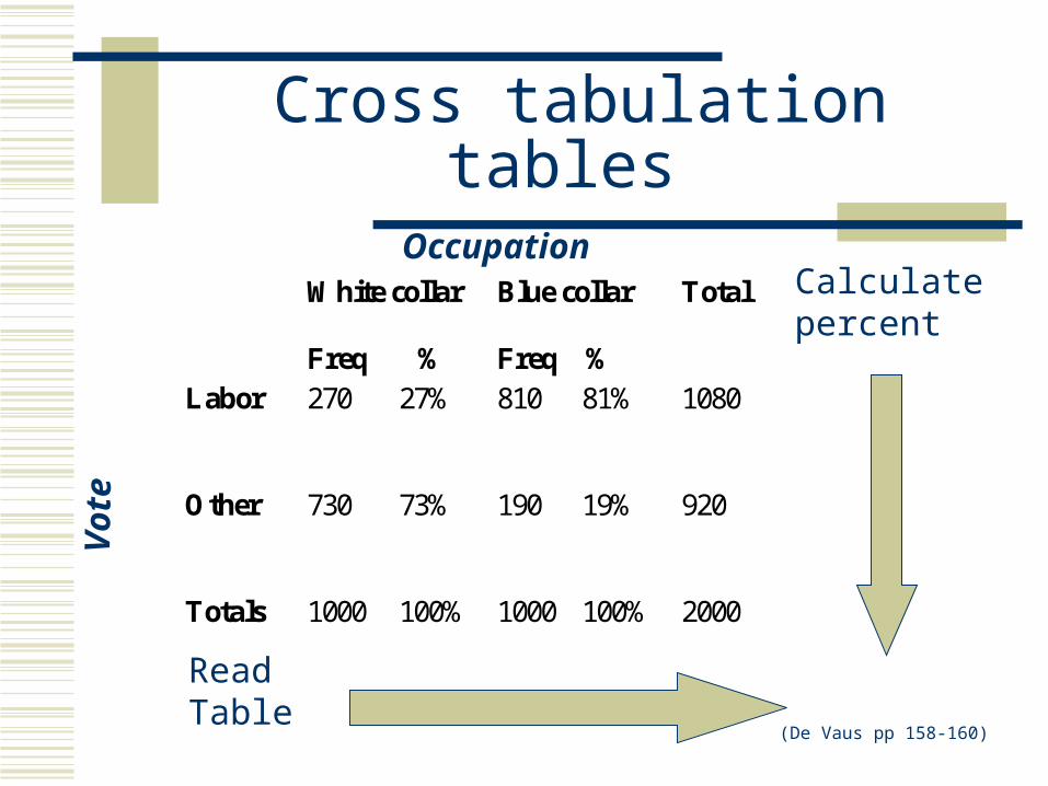
Cross tabulation tables

White collar

Freq %

Blue collar

Freq %

Total

Labor 270 27% 810 81% 1080

Other 730 73% 190 19% 920

Totals 1000 100% 1000 100% 2000

Calculatepercent

ReadTable

(De Vaus pp 158-160)

Occupation

Vote

Cross tabulation

Use column percentages and compare these across the table

Where there is a difference this indicates some association

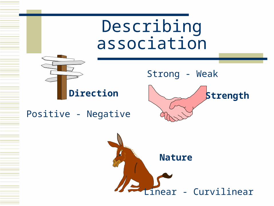
Describing association

Direction Strength

Nature

Positive - Negative

Strong - Weak

Linear - Curvilinear

Describing association

Two variables are positively associated when larger values of one tend to be accompanied by larger values of the other

The variables are negatively associated when larger values of one tend to be accompanied by smaller values of the other

(Moore, p. 254)

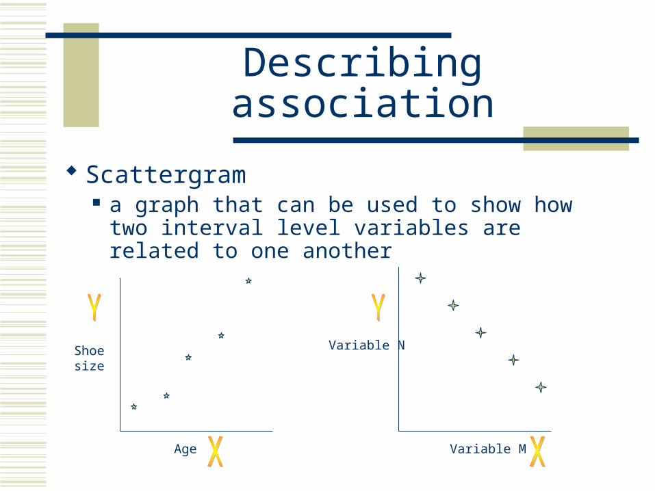
Describing association

Scattergram a graph that can be used to show how two

interval level variables are related to one another

Shoesize

Age

Variable N

Variable M

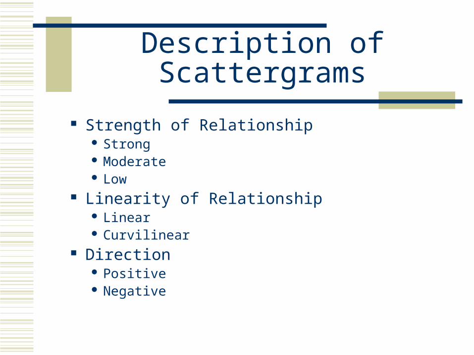
Description of Scattergrams

Strength of Relationship Strong Moderate Low

Linearity of Relationship Linear Curvilinear

Direction Positive Negative

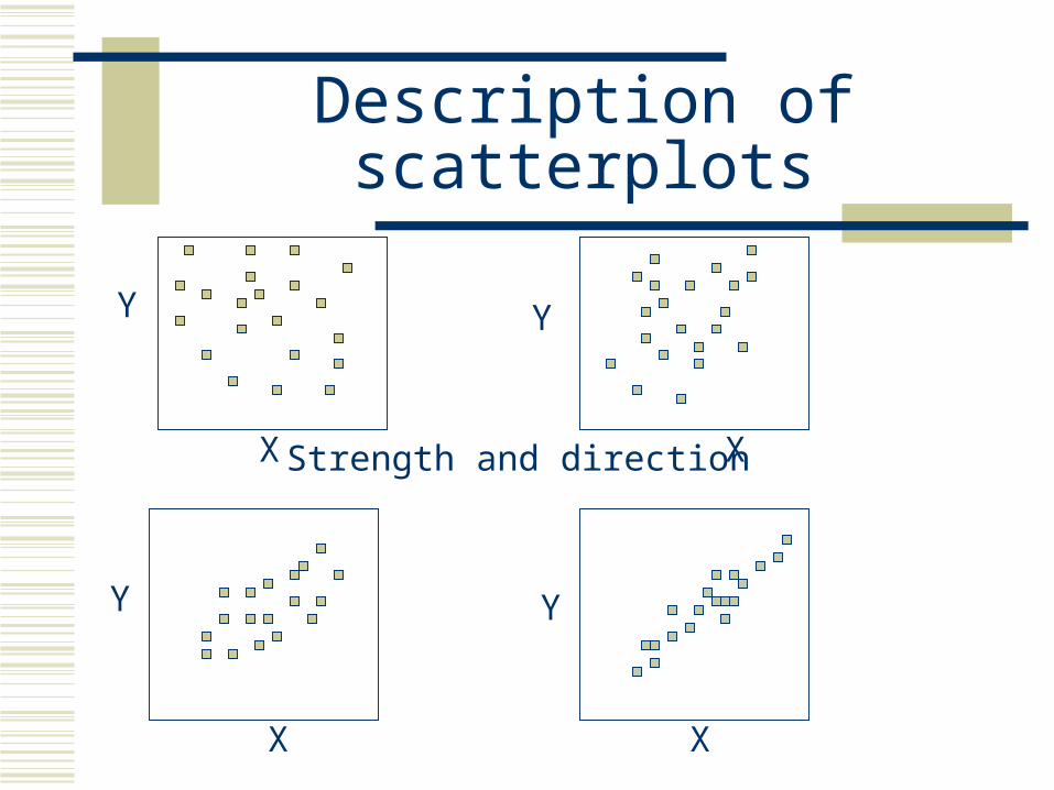
Description of scatterplots

Strength and direction

Y

X X

X X

Y

Y Y

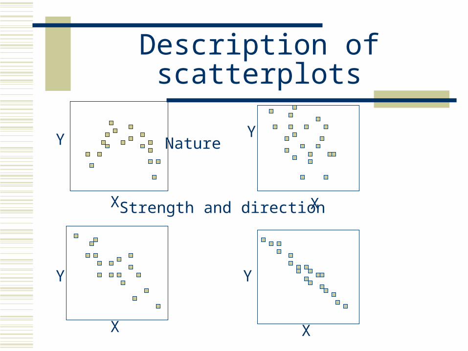
Description of scatterplots

Strength and direction

Nature

X

X X

X

Y

Y Y

Y

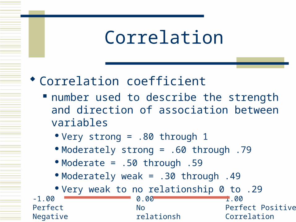
Correlation

Correlation coefficient number used to describe the strength and

direction of association between variablesVery strong = .80 through 1Moderately strong = .60 through .79Moderate = .50 through .59Moderately weak = .30 through .49Very weak to no relationship 0 to .29

-1.00Perfect Negative Correlation

0.00No relationship

1.00 Perfect PositiveCorrelation

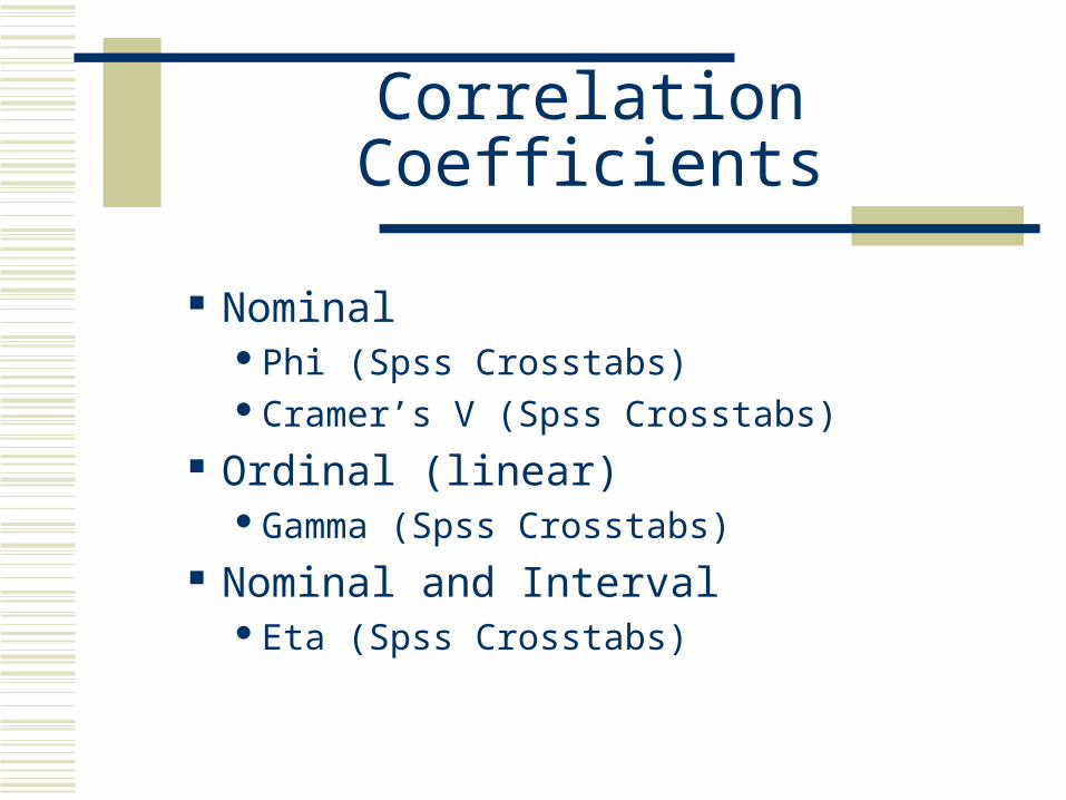
Correlation Coefficients

NominalPhi (Spss Crosstabs)Cramer’s V (Spss Crosstabs)

Ordinal (linear)Gamma (Spss Crosstabs)

Nominal and IntervalEta (Spss Crosstabs)

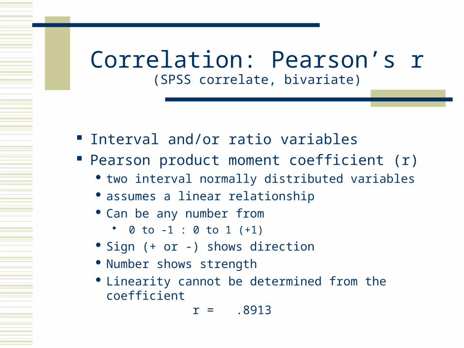
Correlation: Pearson’s r (SPSS correlate, bivariate)

Interval and/or ratio variables Pearson product moment coefficient (r)

two interval normally distributed variables assumes a linear relationship Can be any number from

0 to -1 : 0 to 1 (+1) Sign (+ or -) shows direction Number shows strength Linearity cannot be determined from the coefficient

r = .8913

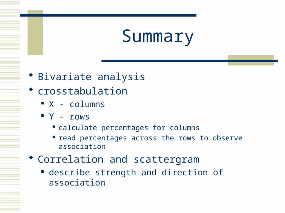
Summary

Bivariate analysis crosstabulation

X - columns Y - rows

calculate percentages for columns read percentages across the rows to observe association

Correlation and scattergram describe strength and direction of association