Embed Size (px)
Citation preview
Form 836 (7/06)
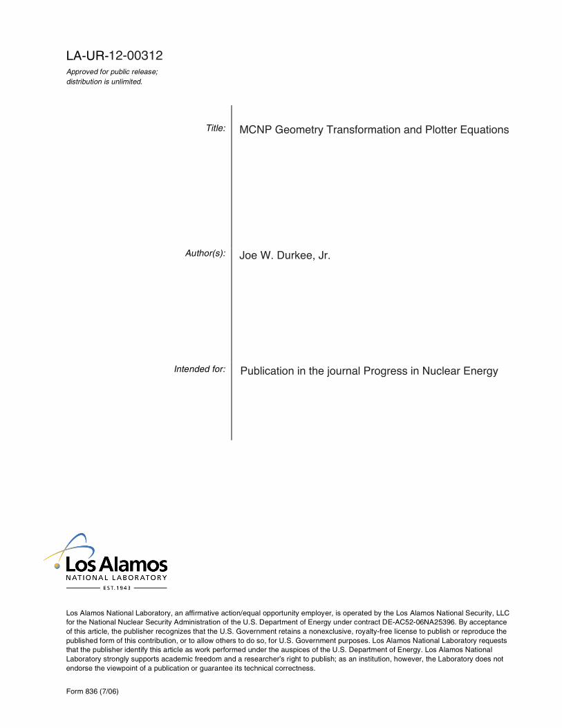
LA-UR- Approved for public release; distribution is unlimited.
Los Alamos National Laboratory, an affirmative action/equal opportunity employer, is operated by the Los Alamos National Security, LLC for the National Nuclear Security Administration of the U.S. Department of Energy under contract DE-AC52-06NA25396. By acceptance of this article, the publisher recognizes that the U.S. Government retains a nonexclusive, royalty-free license to publish or reproduce the published form of this contribution, or to allow others to do so, for U.S. Government purposes. Los Alamos National Laboratory requests that the publisher identify this article as work performed under the auspices of the U.S. Department of Energy. Los Alamos National Laboratory strongly supports academic freedom and a researcher’s right to publish; as an institution, however, the Laboratory does not endorse the viewpoint of a publication or guarantee its technical correctness.
Title:
Author(s):
Intended for:
12-00312
MCNP Geometry Transformation and Plotter Equations
Joe W. Durkee, Jr.
Publication in the journal Progress in Nuclear Energy
1
MCNP GEOMETRY TRANSFORMATION AND PLOTTER EQUATIONS
by
Joe W. Durkee, Jr.Los Alamos National Laboratory
Fax: 505-665-2897PO Box 1663, MS K575Los Alamos, NM 87545
ABSTRACT
The MCNP Monte Carlo radiation-transport code contains versatile capabilities to
develop and plot geometries used in simulations. Although these capabilities have been
available in MCNP since the late 1970s, many of the derivational details underpinning
these capabilities are not contained in the MCNP manual and do not appear to have been
documented in Los Alamos reports or the published literature. Derivations of many of the
equations underlying the MCNP geometry transformation and geometry plot utility are
presented here. Although this document does not include derivations of all of the
expressions contained in MCNP, its contents should nevertheless provide the reader with
a deeper understanding of the geometry transformation and plotting features than can be
obtained using only the MCNP theory manual.
___________________________________________
KEYWORDS: MCNP; geometry; transformation; plot.
2
1. Introduction
Los Alamos National Laboratory (LANL) develops and maintains the MCNP (Brown,
2003) and, prior to the merger, the MCNPXTM(Pelowitz, 2008) Monte Carlo N-Particle
eXtended general-purpose radiation transport codes. We refer here primarily to MCNP
because MCNP and MCNPX contain identical coding related to the subject matter
contained in this document. Some specific mention of MCNPX is made here regarding
the code identifier paradigm used in MCNPX but not in MCNP. A merged version of
MCNP and MCNPX, MCNP6, is expected to be released in 2012. We refer here to
MCNP in general except in instances where specific reference is made to a specific
version of MCNP or to MCNPX.
MCNP accommodates intricate three-dimensional geometrical models, continuous-
energy transport of 34 different particle types plus heavy-ion transport, fuel burnup, and
high-fidelity delayed-gamma emission. MCNP is written in Fortran 90, has been
parallelized, and works on platforms including single-processor personal computers
(PCs), Sun workstations, Linux clusters, and supercomputers. MCNP has approximately
3000 users throughout the world working on endeavors that include radiation therapy,
reactor design, and homeland security.
In the late 1970s the geometry treatment in MCNP was expanded and enhanced. The
MCNP geometry transformation feature dates to the early 1980s (Thompson et. al, 1980),
first appearing in MCNP 2B (Thompson, 1981). This feature provides the user with a
3
convienient and powerful means of specifying surfaces and objects to create problem
geometry. This feature allows surfaces can be created in “local” coordinates, where their
analytic-geometry definitions are simple, and then be moved via translation and/or
rotation operations to their desired “global-coordinate” locations. Beginning with MCNP
2B, the code has possessed the ability to treat geometry transformation using the
coordinate transformation TR card as described in the Coordinate Transformation Card
section of the user’s manuals. In that section, the displacement (“O”) and rotation (“B”)
elements of a geometry transformation are described and their use illustrated. However, it
appears that no documentation exists that explains the derivation of the coordinate
transformation feature.
Visualization of model geometry and of calculated results (“tallies”) is an important
component of the simulation process, particularly when complex models involving multi-
particle transport are being analyzed. Since its creation three decades ago, the MCNP
interactive “PLOT” package has been used to plot model geometry. The “MCPLOT”
package has been used to make two-dimensional (2-D) plots of tally information (i.e.,
calculated fluxes, currents, etc.) and of nuclear cross-section data.
Chapter 2 of the MCNP (Thompson, 1979), MCNP4A (Breismeister, 1993), and
MCNP5 (Brown, 2003a) manuals gives some description and derivational information
about the geometry plotter and how it draws cross-sectional views of the problem
geometry. Included is information discussing the intersection of three-dimensional (3-D)
surfaces with the plot plane and how the surfaces are expressed in plot-plane (s,t)
4
coordinates. Comments and expressions for a set of one-parameter equations for the
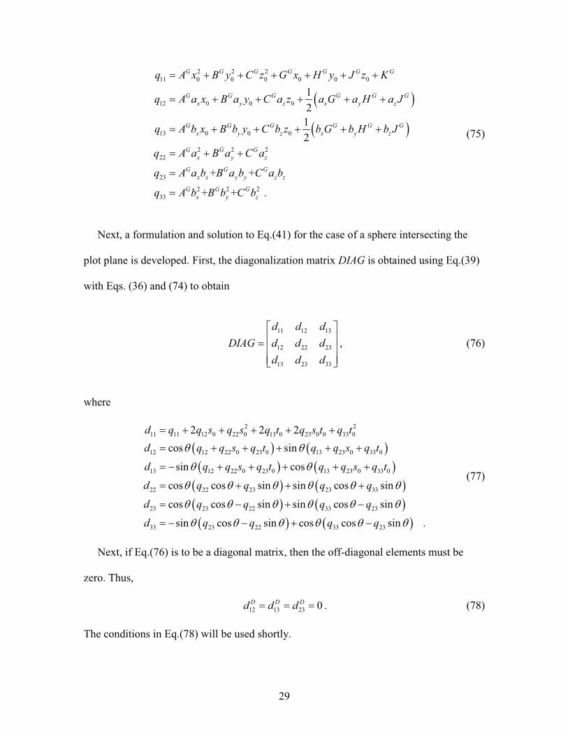
surfaces in the plot plane are then provided without derivation.
In this paper many of the expressions for the geometry transformation and plotting
features are derived. Although the geometry transformation derivation is straightforward,
we will point out an important coding nuance that should be carefully noted by code
developers. The derivation of the plotter equations is not necessary straightforward, and
the derivation of all coded expressions is very lengthy. As such, we present derivations
for an illustrative, yet substantive subset of the cases that have been coded. Included in
the plotter derivation are the one-parameter (“p”) expressions. It is these expressions that
permit plotting of curves in a straightforward manner that is visually appealing, facilitate
the checking whether a surface is within the extent of the plot window, and enable the
checking of the sense with respect to cells bounded by a particular surface. The
derivation of these single-parameter expressions appears not to have previously been
documented in detail. Because they are central to the PLOT package, they are
documented here. During our discussion, specific subroutines and code lines will be
highlighted to help tie the derivations and coding together.
We cite the work of Thomas N. K. Godfrey in developing the geometry translation
and rotation capability for MCNP (Thompson et al., 1980; Thompson, 1981). We also
acknowledge the work that William M. Taylor and Charles A. Forest performed in the
5
1970’s to develop the geometry plotting capability.†
2. Overview of geometry transformation and plotting code flow.
They drew in part from Spain
(2007), a fresh print of which has recently been released by Dover Publications.
During the derivation of the geometry transformation equations, it was discovered that
the theoretical equations differed from the coded expressions in subroutines trfsrf.F,
dunlev.F, etc. In particular, the rotation-component “B” values in the TRF matrix are
transposed relative to the theoretical representation. MCNP corrects this difference via
the transpose operation performed in subroutine trfsrf.F during processing of the input
data. Thus, in effect, MCNP transposes the TRF matrix twice to perform the correct
coordinate-transformation operation. This matter is discussed in detail in Section 3.
The general flow for the geometry transformation and plotting treatment follows. The
reader should also consult the MCNP manuals (Thompson, 1979; Breismeister, 1993;
Brown, 2003a).
Geometry transformations involve individual surfaces (e.g., planes, spheres, etc.) or
macrobodies (e.g., RPP, RCC, etc.) that are specified in “auxiliary” coordinates
( , ,x y z! ! ! ). This convention simplifies specification for objects whose orientation is not
parallel to one of the global-coordinate axes. Specifications for a surface’s geometry
translation and/or rotation are input using the TR card. MCNP uses this transformation to
† Personal communication from John S. Hendricks June 17, 2010 regarding their undocumented contributions. Dr. Hendricks states that name choices of many of the PLOT subroutines were selected by Charles Forest to reflect his appreciation of Latin.
6
locate and orient each surface in ( , ,x y z ), and subsequently uses the global-coordinate
surfaces to do radiation transport and geometry plotting.
MCNP performs geometry plotting by first finding the intersection of each global-
coordinate surface with the plot plane. This requires a transformation from ( , ,x y z )
coordinates to (s,t) plot-plane coordinates. This transformation is transparent to the user
(i.e., no input is required).
The bivariate plot-plane surface intersection equations (line, parabola, hyperbola,
ellipse) are then transformed to a univariate (p) representation. In this form, points of
intersection (POIs) for surfaces in the plot plane are determined. MCNP then identifies
the cells on either side of a line between each POI. Use of the univariate representation
simplifies these tasks as compared to using the bivariate formulation.
The terminology “auxiliary” and ( , ,x y z ) coordinates is historical. In the following
discussion, we use “local” (or object) coordinates† , ,L L Lx y z( ) instead of auxiliary
coordinates and “global” coordinates " #, ,G G Gx y z instead of ( , ,x y z ) coordinates.
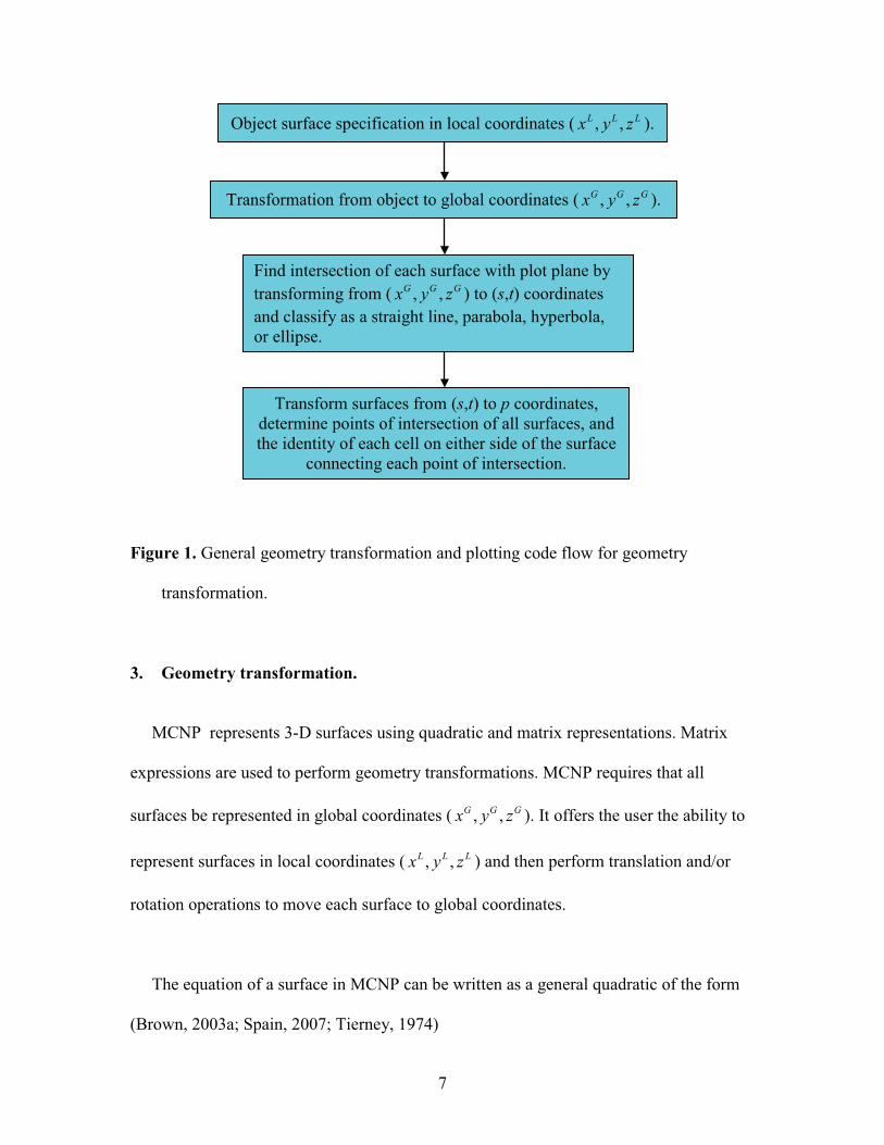
Using this updated terminology, the general geometry and plotting code flow is
sketched in Fig. 1.
† Termed “auxiliary” coordinates ( , ,x y z! ! ! ) in the theory and user’s manuals.
7
Figure 1. General geometry transformation and plotting code flow for geometry
transformation.
3. Geometry transformation.
MCNP represents 3-D surfaces using quadratic and matrix representations. Matrix
expressions are used to perform geometry transformations. MCNP requires that all
surfaces be represented in global coordinates ( , ,G G Gx y z ). It offers the user the ability to
represent surfaces in local coordinates ( , ,L L Lx y z ) and then perform translation and/or
rotation operations to move each surface to global coordinates.
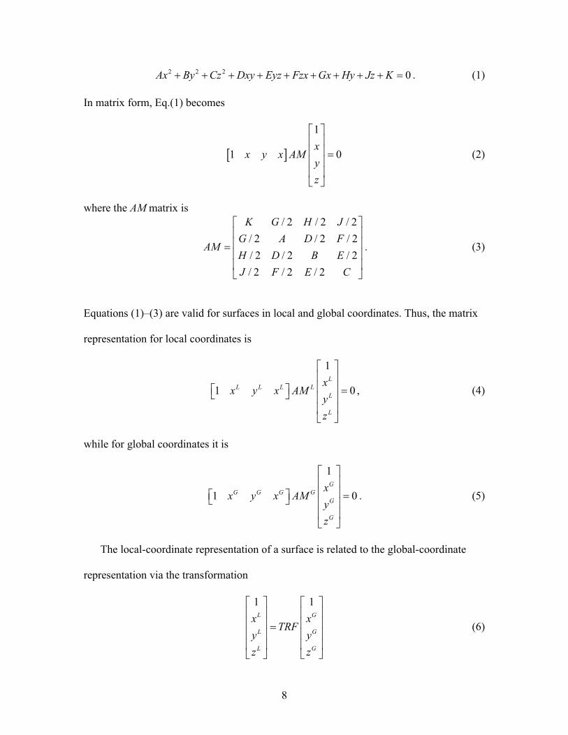
The equation of a surface in MCNP can be written as a general quadratic of the form
(Brown, 2003a; Spain, 2007; Tierney, 1974)
Object surface specification in local coordinates ( , ,L L Lx y z ).
Transformation from object to global coordinates ( , ,G G Gx y z ).
Find intersection of each surface with plot plane by transforming from ( , ,G G Gx y z ) to (s,t) coordinates and classify as a straight line, parabola, hyperbola, or ellipse.
Transform surfaces from (s,t) to p coordinates, determine points of intersection of all surfaces, and the identity of each cell on either side of the surface
connecting each point of intersection.
8
2 2 2 0Ax By Cz Dxy Eyz Fzx Gx Hy Jz K$ $ $ $ $ $ $ $ $ % . (1)
In matrix form, Eq.(1) becomes
& '
1
1 0x
x y x AMyz
( )* +* + %* +* +, -
(2)
where the AM matrix is / 2 / 2 / 2
/ 2 / 2 / 2/ 2 / 2 / 2/ 2 / 2 / 2
K G H JG A D F
AMH D B EJ F E C
( )* +* +%* +* +, -
. (3)
Equations (1)–(3) are valid for surfaces in local and global coordinates. Thus, the matrix
representation for local coordinates is
1
1 0L
L L L LL
L
xx y x AM
yz
( )* +* +( ) %, - * +* +, -
, (4)
while for global coordinates it is
1
1 0G
G G G GG
G
xx y x AM
yz
( )* +* +( ) %, - * +* +, -
. (5)
The local-coordinate representation of a surface is related to the global-coordinate
representation via the transformation
1 1L G
L G
L G
x xTRF
y yz z
( ) ( )* + * +* + * +%* + * +* + * +, - , -
(6)
9
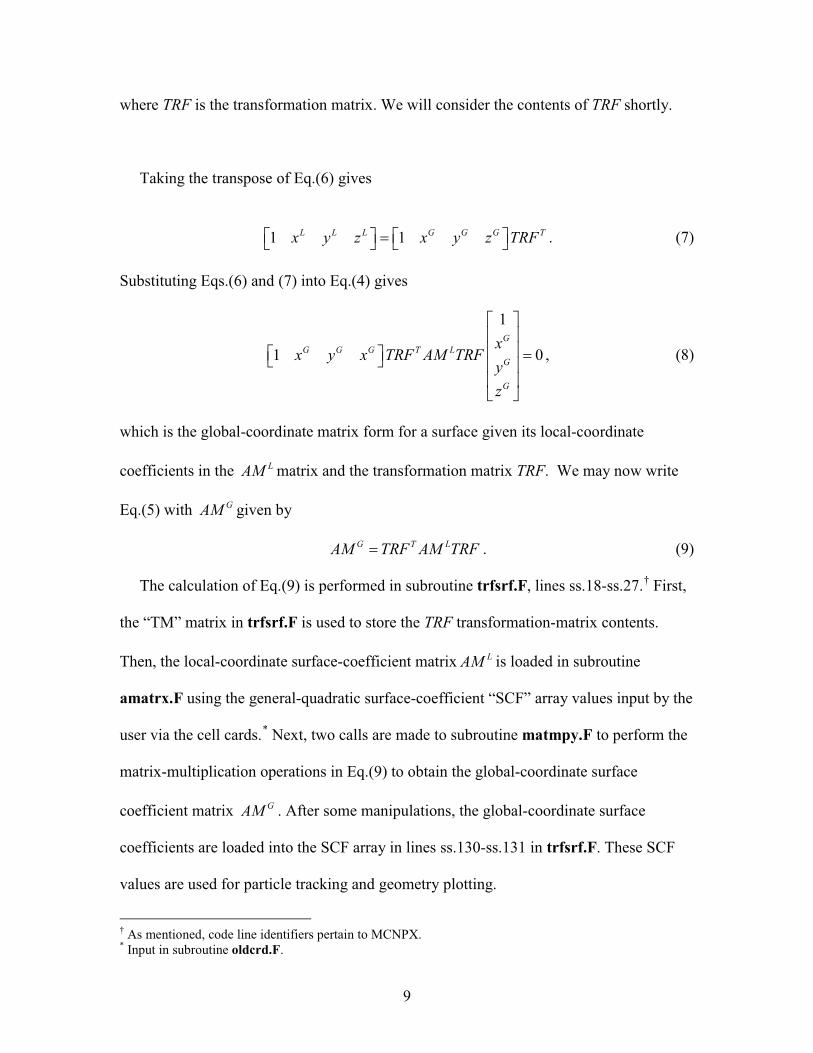
where TRF is the transformation matrix. We will consider the contents of TRF shortly.
Taking the transpose of Eq.(6) gives
1 1L L L G G G Tx y z x y z TRF( ) ( )%, - , - . (7)
Substituting Eqs.(6) and (7) into Eq.(4) gives
1
1 0G
G G G T LG
G
xx y x TRF AM TRF
yz
( )* +* +( ) %, - * +* +, -
, (8)
which is the global-coordinate matrix form for a surface given its local-coordinate
coefficients in the LAM matrix and the transformation matrix TRF. We may now write
Eq.(5) with GAM given by
G T LAM TRF AM TRF% . (9)
The calculation of Eq.(9) is performed in subroutine trfsrf.F, lines ss.18-ss.27.†
LAM
First,
the “TM” matrix in trfsrf.F is used to store the TRF transformation-matrix contents.
Then, the local-coordinate surface-coefficient matrix is loaded in subroutine
amatrx.F using the general-quadratic surface-coefficient “SCF” array values input by the
user via the cell cards.*
GAM
Next, two calls are made to subroutine matmpy.F to perform the
matrix-multiplication operations in Eq.(9) to obtain the global-coordinate surface
coefficient matrix . After some manipulations, the global-coordinate surface
coefficients are loaded into the SCF array in lines ss.130-ss.131 in trfsrf.F. These SCF
values are used for particle tracking and geometry plotting.
† As mentioned, code line identifiers pertain to MCNPX.* Input in subroutine oldcrd.F.
10
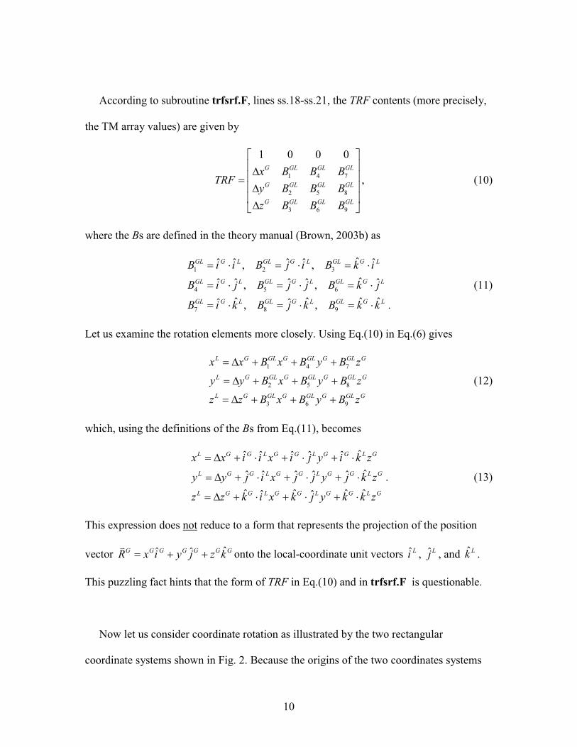
According to subroutine trfsrf.F, lines ss.18-ss.21, the TRF contents (more precisely,
the TM array values) are given by
1 4 7
2 5 8
3 6 9
1 0 0 0G GL GL GL
G GL GL GL
G GL GL GL
x B B BTRF
y B B Bz B B B
( )* +.* +%* +.* +., -
, (10)
where the Bs are defined in the theory manual (Brown, 2003b) as
1 2 3
4 5 6
7 8 9
ˆˆ ˆ ˆ ˆ ˆ, ,ˆˆ ˆ ˆ ˆ ˆ, ,
ˆ ˆ ˆ ˆˆ ˆ, , .
GL G L GL G L GL G L
GL G L GL G L GL G L
GL G L GL G L GL G L
B i i B j i B k i
B i j B j j B k j
B i k B j k B k k
% / % / % /
% / % / % /
% / % / % /
(11)
Let us examine the rotation elements more closely. Using Eq.(10) in Eq.(6) gives
1 4 7
2 5 8
3 6 9
L G GL G GL G GL G
L G GL G GL G GL G
L G GL G GL G GL G
x x B x B y B zy y B x B y B zz z B x B y B z
% . $ $ $
% . $ $ $
% . $ $ $
(12)
which, using the definitions of the Bs from Eq.(11), becomes
ˆˆ ˆ ˆ ˆ ˆˆˆ ˆ ˆ ˆ ˆ
ˆ ˆ ˆ ˆˆ ˆ
L G G L G G L G G L G
L G G L G G L G G L G
L G G L G G L G G L G
x x i i x i j y i k zy y j i x j j y j k zz z k i x k j y k k z
% . $ / $ / $ /
% . $ / $ / $ /
% . $ / $ / $ /
. (13)
This expression does not
ˆˆ ˆG G G G G G GR x i y j z k% $ $!
reduce to a form that represents the projection of the position
vector onto the local-coordinate unit vectors ˆLi , ˆLj , and ˆLk .
This puzzling fact hints that the form of TRF in Eq.(10) and in trfsrf.F is questionable.
Now let us consider coordinate rotation as illustrated by the two rectangular
coordinate systems shown in Fig. 2. Because the origins of the two coordinates systems
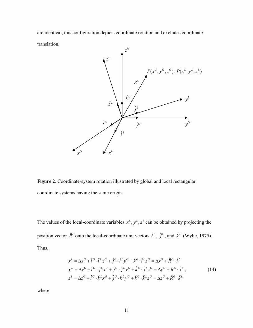
11
are identical, this configuration depicts coordinate rotation and excludes coordinate
translation.
Figure 2. Coordinate-system rotation illustrated by global and local rectangular
coordinate systems having the same origin.
The values of the local-coordinate variables , ,L L Lx y z can be obtained by projecting the
position vector GR!
onto the local-coordinate unit vectors ˆLi , ˆLj , and ˆLk (Wylie, 1975).
Thus,
ˆˆ ˆ ˆ ˆ ˆ ˆˆˆ ˆ ˆ ˆ ˆ ˆ
ˆ ˆ ˆ ˆ ˆˆ ˆ
L G G L G G L G G L G G G L
L G G L G G L G G L G G G L
L G G L G G L G G L G G G L
x x i i x j i y k i z x R iy y i j x j j y k j z y R jz z i k x j k y k k z z R k
% . $ / $ / $ / % . $ /
% . $ / $ / $ / % . $ /
% . $ / $ / $ / % . $ /
!!!
, (14)
where
xG
yG
xL
yL
zL
ˆGi
ˆLi
ˆGj
ˆLj
ˆGkˆLk
GR!
( , , ) : ( , , )G G G L L LP x y z P x y z
zG
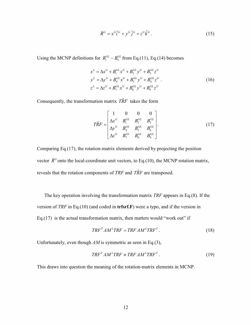
12
ˆˆ ˆG G G G G G GR x i y j z k% $ $!
. (15)
Using the MCNP definitions for 1 9GL GLB B0 from Eq.(11), Eq.(14) becomes
1 2 3
4 5 6
7 8 9
L G GL G GL G GL G
L G GL G GL G GL G
L G GL G GL G GL G
x x B x B y B zy y B x B y B zz z B x B y B z
% . $ $ $
% . $ $ $
% . $ $ $
. (16)
Consequently, the transformation matrix TRF" takes the form
1 2 3
4 5 6
7 8 9
1 0 0 0G GL GL GL
G GL GL GL
G GL GL GL
x B B BTRF
y B B Bz B B B
( )* +.* +%* +.* +., -
" . (17)
Comparing Eq.(17), the rotation-matrix elements derived by projecting the position
vector GR!
onto the local-coordinate unit vectors, to Eq.(10), the MCNP rotation matrix,
reveals that the rotation components of TRF and TRF" are transposed.
The key operation involving the transformation matrix TRF appears in Eq.(8). If the
version of TRF in Eq.(10) (and coded in trfsrf.F) were a typo, and if the version in
Eq.(17) is the actual transformation matrix, then matters would “work out” if
T L L TTRF AM TRF TRF AM TRF% . (18)
Unfortunately, even though AM is symmetric as seen in Eq.(3),
T L L TTRF AM TRF TRF AM TRF1 . (19)
This draws into question the meaning of the rotation-matrix elements in MCNP.
13
The conflict is resolved in MCNP as follows. The Bs from TR cards are input into
nextit.F during rdprob.F processing. Subroutine rdprob.F then calls oldcrd.F, which
calls trfmat.F. Subroutine trfmat.F does several things, including orthonormalizing and
transposing the Bs (TRF matrix) in lines tm4b.15-tm.112. The coding in subroutine
trfsrf.F, lines ss.18-ss.21, transposes the Bs so that the matrix appears as in Eq.(17)
rather than Eq.(10). Thus, MCNP is performing properly, albeit with two (seemingly
unnecessary) transpose operations.
4. Geometry plotter: intersection of 3-D surfaces with the plot plane.
The MCNP geometry plotter draws cross-sectional views of the problem geometry
according to commands entered by the user. MCNP determines the intersection of each
global-coordinate surface with the plot plane. The expressions in the MCNP manuals and
the derivation of these expressions rely on analytic geometry and matrix theory for linear
and quadratic algebraic equations.
From Eq.(1), the equation of an MCNP global-coordinate surface is
2 2 2( ) ( ) ( )0 .
G G G G G G G G G G G G G G G
G G G G G G G
A x B y C z D x y E y z F x zG x H y J z K
$ $ $ $ $
$ $ $ $ %(20)
The surface coefficients G GA K0 are contained in the SCF array as loaded in trfsrf.F
lines ss.130–ss.131.
The equation of the plot plane can be expressed using the parametric representation
for the equation of a plane (Trench, 1972). The plot plane is specified in terms of its
position with respect to the origin and the orientation of its coordinate axes with respect
14
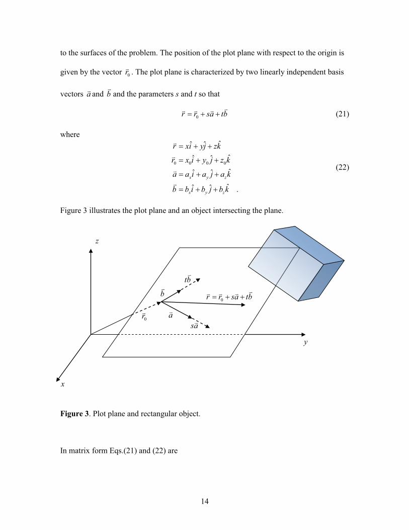
to the surfaces of the problem. The position of the plot plane with respect to the origin is
given by the vector 0r! . The plot plane is characterized by two linearly independent basis
vectors a! and b!
and the parameters s and t so that
0r r sa tb% $ $!! ! ! (21)
where
0 0 0 0
ˆˆ ˆˆˆ ˆˆˆ ˆ
ˆˆ ˆ .x y z
x y z
r xi yj zkr x i y j z k
a a i a j a k
b b i b j b k
% $ $
% $ $
% $ $
% $ $
!!
!!
(22)
Figure 3 illustrates the plot plane and an object intersecting the plane.
Figure 3. Plot plane and rectangular object.
In matrix form Eqs.(21) and (22) are
x
z
y
0r!
b!
tb!
a!
sa!
0r r sa tb% $ $!! ! !
15
0
0
0
1 0 011 1G
x xG
y yG
z z
x a bxs PL s
y a byt t
z a bz
( )( )( ) ( )* +* +* + * +* +* + % %* + * +* +* +* + * +* +* + , - , -
, - , -
(23)
where
0
0
0
1 0 0
x x
y y
z z
x a bPL
y a bz a b
( )* +* +%* +* +, -
. (24)
We seek to develop the expression for intersection of a 3-D surface with the plot
plane. It can be shown that, with the exception of two parallel lines, the intersection of a
plane and a 3-D surface can be written as general bivariate quadratic (Hsiung and Mao,
1998; Kwak and Hong, 1997; Spain, 2007; Tierney, 1974, p.230) in the form (Spain,
2007)
2 22 2 2 0P P P P P PA s H st B t G s F t C$ $ $ $ $ % (25)
using the plot-plane coordinate variables s and t. The superscript “P” is used here to
explicitly connote that these coefficients pertain to the plot-plane conic rather than the
coefficients of the surface intersecting the plot plane. This is the representation of a conic
in the plot plane that is used in MCNP (Brown, 2003a). In matrix form Eq.(25) is
& ' & '1 1
1 1 0
P P P
P P P
P P P
C G Fs t G A H s s t QM s
F H B t t
( ) ( ) ( )* + * + * +% %* + * + * +* + * + * +, - , -, -
. (26)
16
Taking the transpose of Eq.(23)
& '1 1G G G Tx y z s t PL( ) %, - (27)
and substituting into Eq.(2) gives the equation of a 3-D object in terms of plot-plane
coordinates:
& '1
1 0T Gs t PL AM PL st
( )* + %* +* +, -
. (28)
Comparison of Eq.(28) and Eq.(26) shows that
11 12 13
21 22 23
31 32 33
P P P
T G P P P
P P P
C G F q q qQM PL AM PL G A H q q q
F H B q q q
( ) ( )* + * +% % 2* + * +* + * +, -, -
. (29)
Inspection of Eq.(29) shows the QM matrix is both square and symmetric, i.e.,
11 12 13
12 22 23
13 23 33
P P P
T G P P P
P P P
C G F q q qQM PL AM PL G A H q q q
F H B q q q
( ) ( )* + * +% % 2* + * +* + * +, -, -
. (30)
Equation (28) can thus be written as
& '1
1 0s t QM st
( )* + %* +* +, -
, (31)
or in the quadratic form
2 222 23 33 12 13 112 2 2 0q s q st q t q s q t q$ $ $ $ $ % . (32)
Eq. (31) gives the matrix form of the expression for the intersection of a 3-D surface
with the plot plane, i.e., the curve(s) to be plotted. The QM matrix is a matrix of the
coefficients for the quadratic form of the surface(s) in the plot plane. However, these
17
expressions contain two plot variables s and t. The question arises how to select the
values of s and t so that an adequate series of points along the curve(s) can be selected
and plotted using piecewise linear line segments between the points. As pointed out in the
1979 MCNP manual (Thompson, 1979), there is no consistent way to generate the sets of
points that lie on the curve for a two-parameter expression. Instead of a two-parameter
expression, we need a one-parameter representation of Eq.(31) such that, for the
parameter p,
( ), ( ),s s p t t p p% % 03 4 4 3 . (33)
To develop a one-parameter expression, some useful properties of equations and matrices
are used.
Recall that the MCNP geometry-transformation feature (Section 3) takes advantage of
the simplicity with which surfaces can be defined in local coordinates. These surfaces can
be translated and rotated to their general-coordinate locations and used to form objects
with desired locations and orientations. This notion is used for the plotter equations, but
in a reverse sense: equations can have simpler forms if they are translated and/or rotated
to other coordinate systems (Kwak and Hong, 1997; Tierney, 1974 pp. 204–206, 225–
226). We seek to simplify Eq.(31) by translation and/or rotation operations to obtain the
simplest form of the general quadratic equation in an alternate coordinate system.
18
Before considering the translation/rotation matrix, we consider some useful properties
from matrix theory. First, recall that an “elementary transformation” of a matrix is any
one of the following operations (Wylie, p. 491):
a. The multiplication of each element of a row or a column by the same nonzero
constant.
b. The interchange of two rows or of two columns.
c. The addition of any multiple of the elements of one row, or one column, to the
corresponding elements of another row, or column, respectively.
Second, two matrices are “equivalent” if either of these matrices can be obtained from the
other by a series of elementary transformations (Wylie, p. 493). Third, a theorem of
matrix theory is that if A and B are equivalent matrices, then B PAQ% , where P and Q
are nonsingular matrices (Wylie, p. 493). Fourth, a theorem of matrix theory is that any
square matrix is equivalent to a diagonal matrix (Wylie, p. 494). Fifth, a theorem of
matrix theory is that a square matrix is congruent (has the same size and shape) to a
diagonal matrix if and only if it is symmetric, that is TB Q AQ% (Hsiung and Mao, p. 150;
Wylie, p. 549).
These definitions and theorems are used for the MCNP plotter. Because QM matrix is
both square and symmetric, Eq.(30), a single matrix DIA and its transpose†
TDIA QM DIA
can be used to
perform congruence transform (Wylie, p. 497) with the property that is
diagonal (Wylie, p. 549).
† Rather than two nonsingular matrices for a general equivalence transformation.
19
The matrix to be used to effect the congruence transformation and change Eq.(32)
into its simplest form is the general translation and rotation operation matrix in the plot
plane, defined in the u-v coordinate system (Thompson, 1979; Spain, 2007 pp. 62–64;
Tierney, 1974 pp. 204–206, 225–226) †
0
0
1 1 0 0 1cos sinsin cos
s s ut t v
5 55 5
( ) ( ) ( )* + * + * +% 0* + * + * +* + * + * +, - , - , -
(34)
or1 1s DIA ut v
( ) ( )* + * +%* + * +* + * +, - , -
, (35)
where
0
0
1 0 0cos sinsin cos
DIA st
5 55 5
( )* +% 0* +* +, -
. (36)
The DIAG matrix is
11 12 13
21 22 23
31 32 33
,T
d d dDIAG DIA QM DIA d d d
d d d
( )* +% % * +* +, -
(37)
where
† The important details in Eqs.(34)–(37) are omitted from subsequent MCNP manuals.
20
" # " #" # " #" # " #
2 211 11 12 21 0 22 0 13 31 0 23 32 0 0 33 0
12 12 22 0 32 0 13 23 0 33 0
21 21 22 0 23 0 31 32 0 33 0
13 12 22 0 32 0 13 23 0 33 0
31 2
( ) ( ) ( )cos sincos sin
sin cossin
d q q q s q s q q t q q s t q td q q s q t q q s q td q q s q t q q s q td q q s q t q q s q td q
5 55 55 55
% $ $ $ $ $ $ $ $% $ $ $ $ $
% $ $ $ $ $
% 0 $ $ $ $ $
% 0 " # " #" # " #" # " #" # " #" #
1 22 0 23 0 31 23 0 33 0
23 23 22 33 32
32 32 22 33 23
22 22 23 23 33
33 23 22 33
coscos cos sin sin cos sincos cos sin sin cos sincos cos sin sin cos sin
sin cos sin cos cos
q s q t q q s q td q q q qd q q q qd q q q qd q q q q
55 5 5 5 5 55 5 5 5 5 55 5 5 5 5 55 5 5 5 5
$ $ $ $ $
% 0 $ 0
% 0 $ 0
% $ $ $
% 0 0 $ 0" #23 sin .5
(38)
From Eq.(30), symmetry of the QM matrix means that ij jid d% so that
11 12 13
12 22 23
13 23 33
,T
d d dDIAG DIA QM DIA d d d
d d d
( )* +% % * +* +, -
(39)
with 11d simplifying to
2 211 11 12 0 22 0 13 0 23 0 0 33 02 2 2d q q s q s q t q s t q t% $ $ $ $ $ . (40)
Writing the intersection of an MCNP surface with the plot plane as “I,” we take
Eq.(26) and use Eq.(35) to give the intersection of a surface and the plot plane in ( , )u v as
& '1
1 0TI u v DIA QM DIA uv
( )* +% %* +* +, -
. (41)
Using Eq.(39), Eq.(41) expands to
2 211 12 13 23 22 332 2 2 0I d d u d v d uv d u d v% $ $ $ $ $ % . (42)
Equation (42) has the same form as Eq.(25); thus, Eq.(42) is a general bivariate quadratic.
The parameters of the transform, 0s , 0t , and 5 are determined so that
21
the uv term is eliminated from Eq.(42) to give
2 211 12 13 22 332 2 0D D D D D DI d d u d v d u d v% $ $ $ $ % . (43)
Specific forms of Eq.(43) are obtained depending on the type of curve (conic) that is
produced by the intersection of the 3-D surface with the plot plane. The diagonalization
of the QM matrix thus introduces a coordinate system in u and v in which the equations
of the conic sections have their simplest and most symmetric form. The one-parameter set
of relationships is of the form ( )u u p% and ( )v v p% , where p03 4 4 3 . Using the
transformation Eq.(36), we can then obtain ( )s s p% and ( ).t t p%
For use with curves in the plot plane other than straight lines, Eq.(43) is obtained as
follows. There exists an angle D5 , satisfying 0 / 2D5 67 7 , such that a rotation of the
quadratic surface through D5 will cause 23 0Dd % and thereby eliminate term in uv from
Eq.(42).†23dThe expression for in Eq.(38) contains only the angle 5 (not 0s or 0t ), so
we can solve 23 0Dd % for the angle:
" # " #" # " #
" #
23 22 33 23
2 223 33 22
23 33 22
cos cos sin sin cos sin 0
cos sin cos sin 0
1cos 2 sin 2 02
q q q q
q q q
q q q
5 5 5 5 5 5
5 5 5 5
5 5
0 $ 0 %
0 $ 0 %
$ 0 %
(44)
so that the rotation angle D5 which satisfies the diagonalization condition is
1 23
22 33
21 tan2
D qq q
5 0 8 9% : ;0< =
. (45)
† This property is also a mathematical theorem (Tierney, 1974 p. 227).
22
Equation (45) is coded in subroutine regula.F statement rg.67 for use with surfaces in the
plot plane other than straight lines.
To recap, the equation for the intersection of an MCNP surface given by Eq.(20) with
the plot plane is a conic given by Eq.(25). The equation for this conic can be written in
matrix form given by Eq.(26). This bivariate expression can be recast as a univariate
expression by the use of a general translation and rotation operation in the plot plane as
given by Eqs.(35) and (36). The univariate expression is suitable for plotting purposes.
We will use the diagonalization condition in Eq.(39) with a determination of the
transform parameters 0s , 0t , and 5 to obtain the conditions that cause 0DI % in Eq.(43)
for four types of conics in the plot plane. First we will treat cases where a plane and a
sphere intersect the plot plane. The intersection of a plane with the plot plane produces a
line, whereas a sphere creates a circle, ellipse, or a point. The intersection of other types
of surfaces with the plot plane causing a hyperbola or a parabola will then be examined.
4.1. Intersection of a plane with the plot plane
To illustrate the procedure for developing a one-parameter expression for a 3-D
surface in the plot plane, let us consider the 3-D surface to be a plane. Intuitively, the
intersection will be a line. For a plane, Eq.(20) becomes
0G G G G G G GG x H y J z K$ $ $ % , (46)
so that the matrix representation given by Eq.(5),
23
1
1 0G
G G G GG
G
xx y x AM
yz
( )* +* +( ) %, - * +* +, -
, (47)
has the coefficient matrix given by Eq. (3) written as
/ 2 / 2 / 2/ 2 0 0 0/ 2 0 0 0/ 2 0 0 0
G G G G
GG
G
G
K G H JGAMHJ
( )* +* +%* +* +, -
. (48)
The expression for the plane in plot-plane coordinates is given by Eq.(31) with
0 0 0 2 2 2 2 2 2
0 02 2 2
0 02 2 2
G GG GG Gy yG G G G x xz z
GG Gyx z
GG Gyx z
a H b Ha G b Ga J b JK G x H y J z
a Ha G a JQM
b Hb G b J
( )$ $ $ $ $ $ $* +
* +* +
% $ $* +* +* +
$ $* +* +, -
(49)
or 11 12 13
21
31
0 00 0
q q qQM q
q
( )* +% * +* +, -
(50)
or, noting the symmetry,11 12 13
12
13
0 00 0
q q qQM q
q
( )* +% * +* +, -
(51)
where
24
11 0 0 0
12
13
2 2 2
.2 2 2
G G G G
GG Gyx z
GG Gyx z
q K G x H y J za Ha G a Jq
b Hb G b Jq
% $ $ $
% $ $
% $ $
(52)
We next seek to formulate and solve Eq.(41) for the case of a plane intersecting the
plot plane. First, the diagonalization matrix DIAG is obtained using Eq.(39) with Eqs.
(36) and (51) so that (Mathematica, 1991)
11 12 0 21 0 13 0 31 0 12 13 13 12
12 13
13 12
cos sin cos sincos sin 0 0cos sin 0 0
TDIAG DIA QM DIAq q s q s q t q t q q q q
q qq q
5 5 5 55 55 5
%$ $ $ $ $ 0( )
* +% $* +* +0, -
(53)
or, noting the symmetry in Eq.(53),11 12 13
12 22 23
13 23 33
,d d d
DIAG d d dd d d
( )* +% * +* +, -
(54)
where
11 11 12 0 21 0 13 0 31 0
12 12 13
13 13 12
cos sincos sin ,
d q q s q s q t q td q qd q q
5 55 5
% $ $ $ $% $% 0
(55)
and
22 23 33 0D D Dd d d% % % . (56)
Next, if Eq.(53) is to be a diagonal matrix, then the off-diagonal elements must be
zero. From Eq.(53)–(55), this means that we have the conditions
12 13 0D Dd d% % , (57)
so that
25
12
13
13
12
cos sin
cos sin ,
5 5
5 5
%
% 0(58)
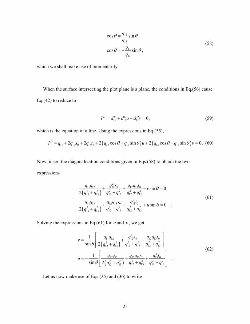
which we shall make use of momentarily.
When the surface intersecting the plot plane is a plane, the conditions in Eq.(56) cause
Eq.(42) to reduce to
11 12 13 0D D D DI d d u d v% $ $ % , (59)
which is the equation of a line. Using the expressions in Eq.(55),
" # " #11 12 0 13 0 12 13 13 122 2 2 cos sin 2 cos sin 0DI q q s q t q q u q q v5 5 5 5% $ $ $ $ $ 0 % . (60)
Now, insert the diagonalization conditions given in Eqs.(58) to obtain the two
expressions
" #
" #
212 0 12 13 011 12
2 2 2 22 212 13 12 1312 13
211 13 12 13 0 13 0
2 2 2 22 212 13 12 1312 13
sin 02
sin 0 .2
q s q q tq q vq q q qq q
q q q q s q t uq q q qq q
5
5
$ $ 0 %$ $$
$ $ $ %$ $$
(61)
Solving the expressions in Eq.(61) for u and v , we get
" #
" #
212 0 12 13 011 12
2 2 2 22 212 13 12 1312 13
211 13 12 13 0 13 0
2 2 2 22 212 13 12 1312 13
1sin 2
1 .sin 2
q s q q tq qvq q q qq q
q q q q s q tuq q q qq q
5
5
( )* +% $ $
$ $$* +, -( )* +% 0 $ $
$ $$* +, -
(62)
Let us now make use of Eqs.(35) and (36) to write
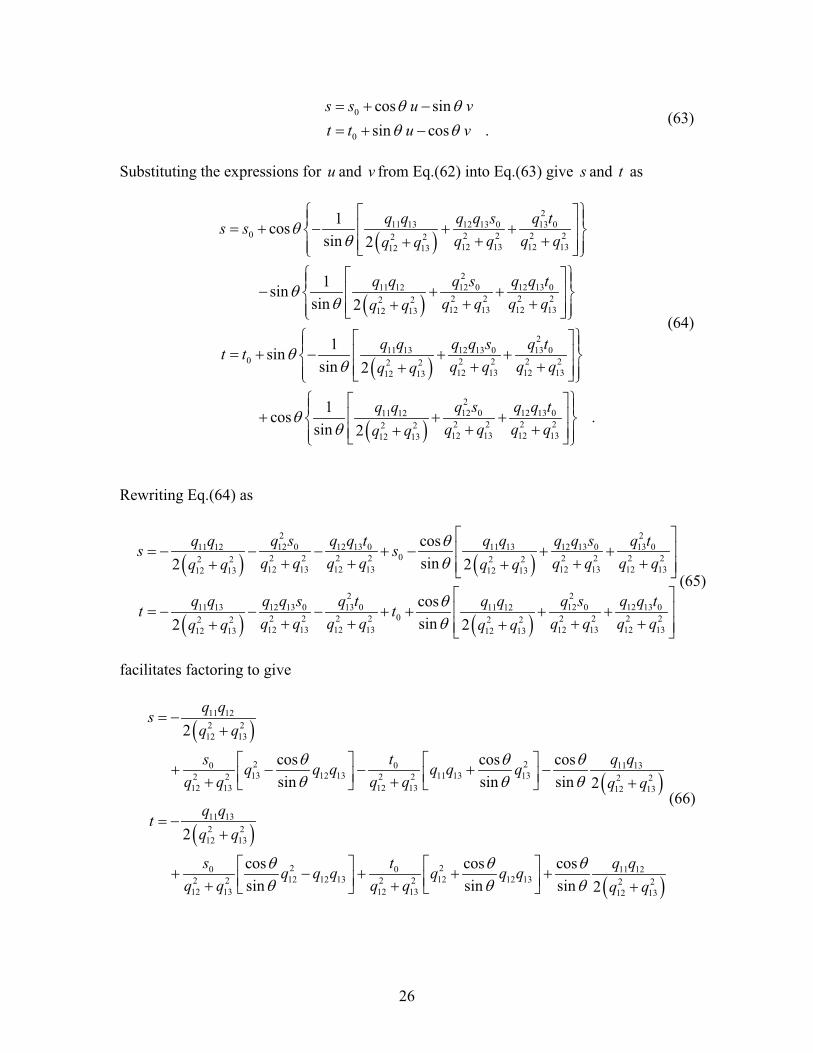
26
0
0
cos sinsin cos .
s s u vt t u v
5 55 5
% $ 0% $ 0
(63)
Substituting the expressions for u and v from Eq.(62) into Eq.(63) give s and t as
" #
" #
" #
211 13 12 13 0 13 0
0 2 2 2 22 212 13 12 1312 13
212 0 12 13 011 12
2 2 2 22 212 13 12 1312 13
11 13 12 130 2 2
12 13
1cossin 2
1sinsin 2
1sinsin 2
q q q q s q ts sq q q qq q
q s q q tq qq q q qq q
q q q q st tq q
55
55
55
> ?( )@ @* +% $ 0 $ $A B$ $$* +@ @, -C D> ?( )@ @* +0 $ $A B$ $$* +@ @, -C D
% $ 0 $$
" #
20 13 0
2 2 2 212 13 12 13
212 0 12 13 011 12
2 2 2 22 212 13 12 1312 13
1cos .sin 2
q tq q q q
q s q q tq qq q q qq q
55
> ?( )@ @* +$A B$ $* +@ @, -C D> ?( )@ @* +$ $ $A B$ $$* +@ @, -C D
(64)
Rewriting Eq.(64) as
" # " #
" #
2 212 0 12 13 0 11 13 12 13 0 13 011 12
02 2 2 2 2 2 2 22 2 2 212 13 12 13 12 13 12 1312 13 12 13
211 13 12 13 0 13 0 11 12
02 2 2 22 2 212 13 12 1312 13 12
cossin2 2
cossin2 2
q s q q t q q q q s q tq qs sq q q q q q q qq q q q
q q q q s q t q qt tq q q qq q q
55
55
( )* +% 0 0 0 $ 0 $ $
$ $ $ $$ $* +, -
% 0 0 0 $ $$ $$ $" #
212 0 12 13 0
2 2 2 2212 13 12 1313
q s q q tq q q qq
( )* +$ $
$ $* +, -
(65)
facilitates factoring to give
" #
" #
" #
11 122 212 13
2 20 0 11 1313 12 13 11 13 132 2 2 2 2 2
12 13 12 13 12 13
11 132 212 13
2 20 012 12 13 122 2 2 2
12 13 12 13
2
cos cos cossin sin sin 2
2
cos cossin sin
q qsq q
s t q qq q q q q qq q q q q q
q qtq q
s tq q q q qq q q q
5 5 55 5 5
5 55 5
% 0$
( ) ( )$ 0 0 $ 0* + * +$ $ $, - , -
% 0$
( )$ 0 $ $* +$ $, - " #11 12
12 13 2 212 13
cossin 2
q qqq q
55
( ) $* + $, -
(66)
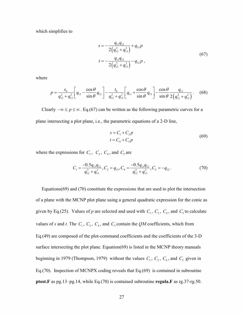
27
which simplifies to
" #
" #
11 12132 2
12 13
11 13122 2
12 13
2
,2
q qs q pq qq qt q pq q
% 0 $$
% 0 0$
(67)
where
" #0 0 11
13 12 11 132 2 2 2 2 212 13 12 13 12 13
cos cos cossin sin sin 2
s t qp q q q qq q q q q q
5 5 55 5 5
( ) ( )% 0 0 $ 0* + * +$ $ $, - , -. (68)
Clearly p03 4 4 3 . Eq.(67) can be written as the following parametric curves for a
plane intersecting a plot plane, i.e., the parametric equations of a 2-D line,
1 2
4 5
s C C pt C C p% $% $
(69)
where the expressions for 1C , 2C , 4C , and 5C are
11 1311 121 2 13 4 5 122 2 2 2
12 13 12 13
0.50.5 , , ,q qq qC C q C C qq q q q
00% % % % 0$ $
. (70)
Equations(69) and (70) constitute the expressions that are used to plot the intersection
of a plane with the MCNP plot plane using a general quadratic expression for the conic as
given by Eq.(25). Values of p are selected and used with 1C , 2C , 4C , and 5C to calculate
values of s and t. The 1C , 2C , 4C , and 5C contain the QM coefficients, which from
Eq.(49) are composed of the plot-command coefficients and the coefficients of the 3-D
surface intersecting the plot plane. Equation(69) is listed in the MCNP theory manuals
beginning in 1979 (Thompson, 1979) without the values 1C , 2C , 4C , and 5C given in
Eq.(70). Inspection of MCNPX coding reveals that Eq.(69) is contained in subroutine
ptost.F as pg.13–pg.14, while Eq.(70) is contained subroutine regula.F as rg.37-rg.50.
28
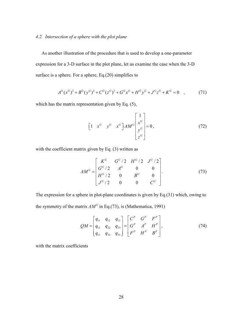
4.2. Intersection of a sphere with the plot plane
As another illustration of the procedure that is used to develop a one-parameter
expression for a 3-D surface in the plot plane, let us examine the case when the 3-D
surface is a sphere. For a sphere, Eq.(20) simplifies to
2 2 2( ) ( ) ( ) 0 ,G G G G G G G G G G G G GA x B y C z G x H y J z K$ $ $ $ $ $ % (71)
which has the matrix representation given by Eq. (5),
1
1 0G
G G G GG
G
xx y x AM
yz
( )* +* +( ) %, - * +* +, -
, (72)
with the coefficient matrix given by Eq. (3) written as
/ 2 / 2 / 2/ 2 0 0/ 2 0 0/ 2 0 0
G G G G
G GG
G G
G G
K G H JG AAMH BJ C
( )* +* +%* +* +, -
. (73)
The expression for a sphere in plot-plane coordinates is given by Eq.(31) which, owing to
the symmetry of the matrix GAM in Eq.(73), is (Mathematica, 1991)
11 12 13
12 22 23
13 23 33
P P P
P P P
P P P
q q q C G FQM q q q G A H
q q q F H B
( )( )* +* +% % * +* +* +* +, - , -
, (74)
with the matrix coefficients
29
" #
" #
2 2 211 0 0 0 0 0 0
12 0 0 0
13 0
2 2 2
23
3
0 0
22
2 2 23
1212
++
+ +
.
G G G G G G G
G G G G G Gx y z x y z
G G G G G Gx y z x
G G Gx y z
G Gx y z
G G
y z
Gx y z
Gx y z
q A x B y C z G x H y J z K
q A a x B a y C a z a G a H a J
q A b x B b y C b z b G b H
A a B a C a
q A a B
b J
q
b b C b
b b C
a a
q A B b
$
% $ $ $ $ $ $
% $
$
%
$ $ $ $
$ $ $ $
%
%
% $ (75)
Next, a formulation and solution to Eq.(41) for the case of a sphere intersecting the
plot plane is developed. First, the diagonalization matrix DIAG is obtained using Eq.(39)
with Eqs. (36) and (74) to obtain
11 12 13
12 22 23
13 23 33
d d dDIAG d d d
d d d
( )* +% * +* +, -
, (76)
where
" # " #" # " #
" # " #" #
2 211 11 12 0 22 0 13 0 23 0 0 33 0
12 12 22 0 23 0 13 23 0 33 0
13 12 22 0 23 0 13 23 0 33 0
22 22 23 23 33
23 23 22
2 2 2cos sin
sin coscos cos sin sin cos sincos cos sin si
d q q s q s q t q s t q td q q s q t q q s q td q q s q t q q s q td q q q qd q q
5 55 5
5 5 5 5 5 55 5 5
% $ $ $ $ $% $ $ $ $ $
% 0 $ $ $ $ $
% $ $ $
% 0 $ " #" # " #
33 23
33 23 22 33 23
n cos sinsin cos sin cos cos sin .
q qd q q q q
5 5 55 5 5 5 5 5
0
% 0 0 $ 0
(77)
Next, if Eq.(76) is to be a diagonal matrix, then the off-diagonal elements must be
zero. Thus,
12 13 23 0D D Dd d d% % % . (78)
The conditions in Eq.(78) will be used shortly.
30
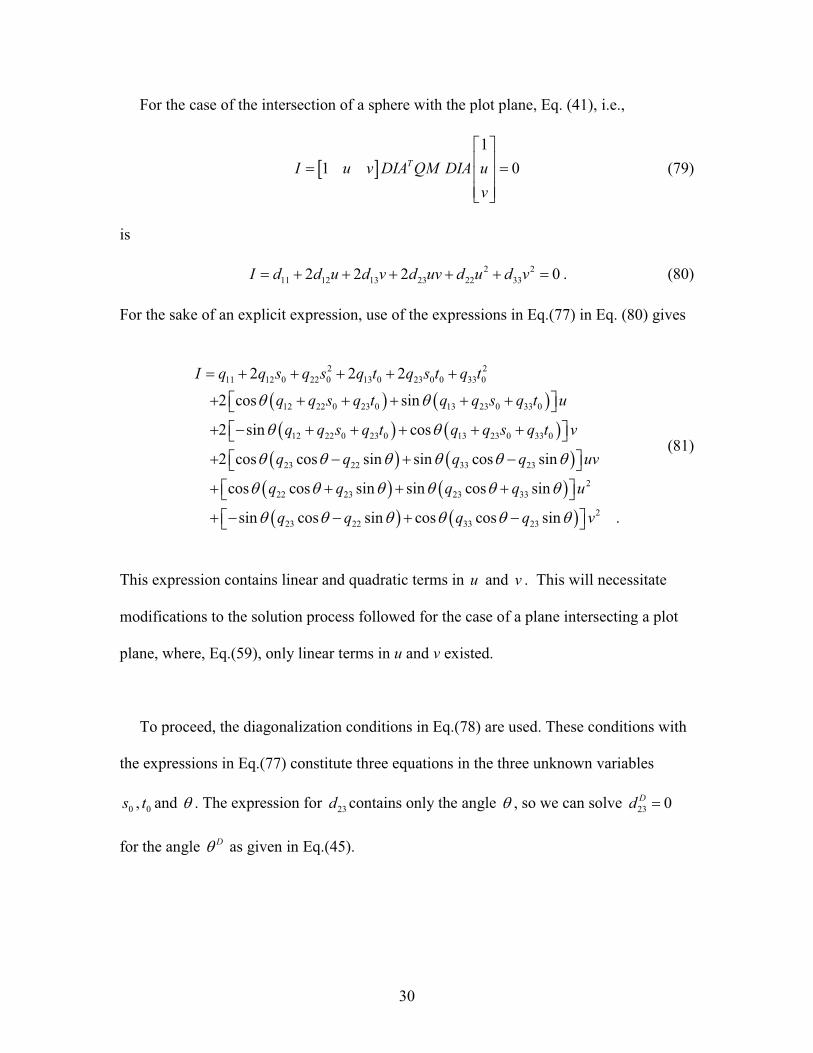
For the case of the intersection of a sphere with the plot plane, Eq. (41), i.e.,
& '1
1 0TI u v DIA QM DIA uv
( )* +% %* +* +, -
(79)
is
2 211 12 13 23 22 332 2 2 0I d d u d v d uv d u d v% $ $ $ $ $ % . (80)
For the sake of an explicit expression, use of the expressions in Eq.(77) in Eq. (80) gives
" # " #" # " #
" # " #
2 211 12 0 22 0 13 0 23 0 0 33 0
12 22 0 23 0 13 23 0 33 0
12 22 0 23 0 13 23 0 33 0
23 22 33 23
22 23
2 2 22 cos sin
2 sin cos
2 cos cos sin sin cos sin
cos cos si
I q q s q s q t q s t q tq q s q t q q s q t u
q q s q t q q s q t v
q q q q uv
q q
5 5
5 5
5 5 5 5 5 5
5 5
% $ $ $ $ $
$ $ $ $ $ $( ), -$ 0 $ $ $ $ $( ), -$ 0 $ 0( ), -$ $" # " #
" # " #
223 33
223 22 33 23
n sin cos sin
sin cos sin cos cos sin .
q q u
q q q q v
5 5 5 5
5 5 5 5 5 5
$ $( ), -$ 0 0 $ 0( ), -
(81)
This expression contains linear and quadratic terms in u and v . This will necessitate
modifications to the solution process followed for the case of a plane intersecting a plot
plane, where, Eq.(59), only linear terms in u and v existed.
To proceed, the diagonalization conditions in Eq.(78) are used. These conditions with
the expressions in Eq.(77) constitute three equations in the three unknown variables
0s , 0t and 5 . The expression for 23d contains only the angle 5 , so we can solve 23 0Dd %
for the angle D5 as given in Eq.(45).
31
Next, we substitute the angle D5 from Eq.(45) into the expressions for 12d and 13d in
Eq.(77) to obtain two coupled equations involving the two unknowns 0s and 0t . Solving
these equations gives (after some algebra)
13 23 12 330 2
22 33 23
q q q qsq q q
0%0
(82)
12 23 13 220 2
22 33 23
q q q qtq q q
0%0
(83)
as the values for the translation involved in the diagonalization process. These values are
coded in subroutine regula.F as rg.77 and rg.78.
With the diagonalization conditions of Eq.(78) and the diagonalization parameters in
Eqs.(45), (82), and (83), the equation of the conic for a sphere intersecting the plot plane
given by Eq.(80) reduces to
2 211 22 33 0D D D DI d d u d v% $ $ % , (84)
where 11Dd , 22
Dd , and 33Dd are 11d , 22d , and 33d given in Eq.(77) evaluated using the
diagonalization parameters D5 , 0s , and 0t given in Eqs. (45), (82), and (83). The
diagonalization process means that Eq.(84) can be written using a one-parameter set of
relationships of the form ( )u u p% and ( )v v p% . So expressions for ( )u u p% and
( )v v p% are sought which satisfy Eq.(84).
In general, the form of ( )u u p% and ( )v v p% is dependent upon the signs of 11Dd , 22
Dd ,
and 33Dd . It can be shown from analytic geometry (Tierney, pp. 226–230) that the
following conics exist:
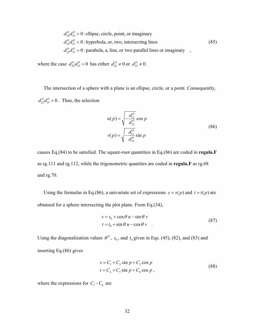
32
22 33
22 33
22 33
0 : ellipse, circle, point, or imaginary0 : hyperbola, or, two, intersecting lines0 : parabola, a, line, or two parallel lines or imaginary ,
D D
D D
D D
d dd dd d
E
7
%
(85)
where the case 22 33 0D Dd d % has either 22 0Dd 1 or 33 0Dd 1 .
The intersection of a sphere with a plane is an ellipse, circle, or a point. Consequently,
22 33 0D Dd d E . Thus, the selection
11
22
11
33
( ) cos
( ) sin
D
D
D
D
du p pd
dv p pd
% 0
% 0
(86)
causes Eq.(84) to be satisfied. The square-root quantities in Eq.(86) are coded in regula.F
as rg.111 and rg.112, while the trigonometric quantites are coded in regula.F as rg.68
and rg.70.
Using the formulas in Eq.(86), a univariate set of expressions ( )s s p% and ( )t t p% are
obtained for a sphere intersecting the plot plane. From Eq.(34),
0
0
cos sinsin cos .
s s u vt t u v
5 55 5
% $ 0% $ 0
(87)
Using the diagonalization values D5 , 0s , and 0t given in Eqs. (45), (82), and (83) and
inserting Eq.(86) gives
1 2 3
4 5 6
sin cossin cos ,
s C C p C pt C C p C p% $ $% $ $
(88)
where the expressions for 1C – 6C are
33
11 111 0 2 3
33 22
11 114 0 5 6
33 22
, sin , cos
, cos , sin ,
D DD D
D D
D DD D
D D
d dC s C Cd d
d dC t C Cd d
5 5
5 5
% % 0 0 % 0
% % 0 0 % 0
(89)
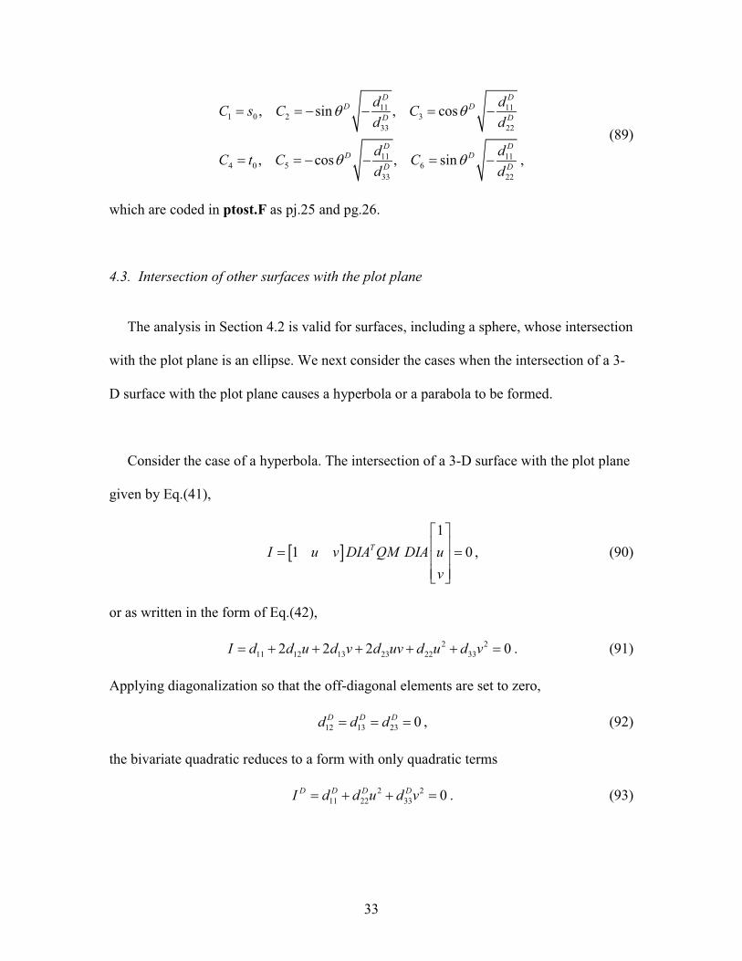
which are coded in ptost.F as pj.25 and pg.26.
4.3. Intersection of other surfaces with the plot plane
The analysis in Section 4.2 is valid for surfaces, including a sphere, whose intersection
with the plot plane is an ellipse. We next consider the cases when the intersection of a 3-
D surface with the plot plane causes a hyperbola or a parabola to be formed.
Consider the case of a hyperbola. The intersection of a 3-D surface with the plot plane
given by Eq.(41),
& '1
1 0TI u v DIA QM DIA uv
( )* +% %* +* +, -
, (90)
or as written in the form of Eq.(42),
2 211 12 13 23 22 332 2 2 0I d d u d v d uv d u d v% $ $ $ $ $ % . (91)
Applying diagonalization so that the off-diagonal elements are set to zero,
12 13 23 0D D Dd d d% % % , (92)
the bivariate quadratic reduces to a form with only quadratic terms
2 211 22 33 0D D D DI d d u d v% $ $ % . (93)
34
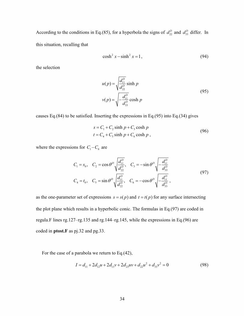
According to the conditions in Eq.(85), for a hyperbola the signs of 22Dd and 33
Dd differ. In
this situation, recalling that
2 2cosh sinh 1x x0 % , (94)
the selection
11
22
11
33
( ) sinh
( ) cosh
D
D
D
D
du p pd
dv p pd
%
% 0
(95)
causes Eq.(84) to be satisfied. Inserting the expressions in Eq.(95) into Eq.(34) gives
1 2 3
4 5 6
sinh coshsinh cosh ,
s C C p C pt C C p C p% $ $% $ $
(96)
where the expressions for 1C – 6C are
11 111 0 2 3
22 33
11 114 0 5 6
22 33
, cos , sin
, sin , cos ,
D DD D
D D
D DD D
D D
d dC s C Cd d
d dC t C Cd d
5 5
5 5
% % % 0 0
% % % 0 0
(97)
as the one-parameter set of expressions ( )s s p% and ( )t t p% for any surface intersecting
the plot plane which results in a hyperbolic conic. The formulas in Eq.(97) are coded in
regula.F lines rg.127–rg.135 and rg.144–rg.145, while the expressions in Eq.(96) are
coded in ptost.F as pj.32 and pg.33.
For the case of a parabola we return to Eq.(42),
2 211 12 13 23 22 332 2 2 0I d d u d v d uv d u d v% $ $ $ $ $ % (98)
35
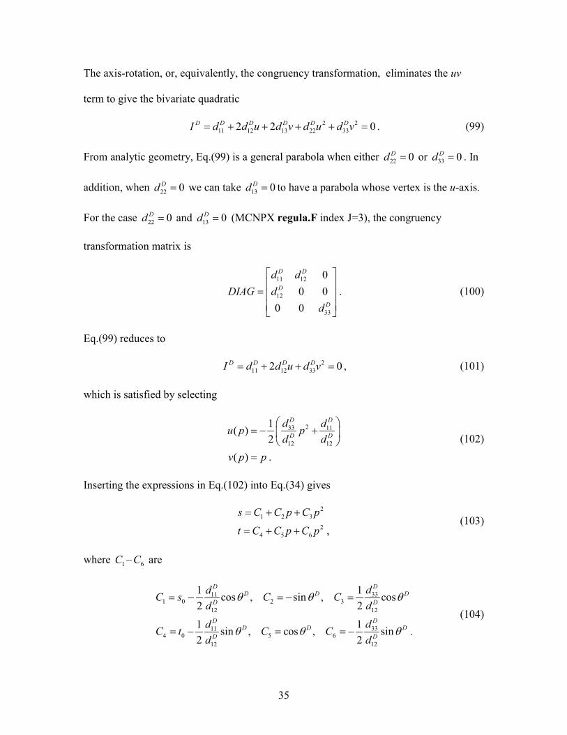
The axis-rotation, or, equivalently, the congruency transformation, eliminates the uv
term to give the bivariate quadratic
2 211 12 13 22 332 2 0D D D D D DI d d u d v d u d v% $ $ $ $ % . (99)
From analytic geometry, Eq.(99) is a general parabola when either 22 0Dd % or 33 0Dd % . In
addition, when 22 0Dd % we can take 13 0Dd % to have a parabola whose vertex is the u-axis.
For the case 22 0Dd % and 13 0Dd % (MCNPX regula.F index J=3), the congruency
transformation matrix is
11 12
12
33
00 0
0 0
D D
D
D
d dDIAG d
d
( )* +% * +* +, -
. (100)
Eq.(99) reduces to
211 12 332 0D D D DI d d u d v% $ $ % , (101)
which is satisfied by selecting
233 11
12 12
1( )2
( ) .
D D
D Dd du p pd d
v p p
8 9% 0 $: ;
< =%
(102)
Inserting the expressions in Eq.(102) into Eq.(34) gives
21 2 3
24 5 6 ,
s C C p C pt C C p C p% $ $
% $ $(103)
where 1C – 6C are
33111 0 2 3
12 12
33114 0 5 6
12 12
1 1cos , sin , cos2 21 1sin , cos , sin .2 2
DDD D D
D D
DDD D D
D D
ddC s C Cd d
ddC t C Cd d
5 5 5
5 5 5
% 0 % 0 %
% 0 % % 0(104)
36
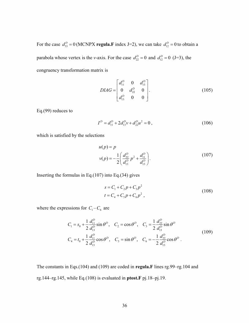
For the case 33 0Dd % (MCNPX regula.F index J=2), we can take 12 0Dd % to obtain a
parabola whose vertex is the v-axis. For the case 22 0Dd % and 12 0Dd % (J=3), the
congruency transformation matrix is
11 13
22
13
00 0
0 0
D D
D
D
d dDIAG d
d
( )* +% * +* +, -
. (105)
Eq.(99) reduces to
211 13 222 0D D D DI d d v d u% $ $ % , (106)
which is satisfied by the selections
222 11
13 13
( )
1( ) .2
D D
D D
u p pd dv p pd d
%
8 9% 0 $: ;
< =
(107)
Inserting the formulas in Eq.(107) into Eq.(34) gives
21 2 3
24 5 6 ,
s C C p C pt C C p C p% $ $
% $ $(108)
where the expressions for 1C – 6C are
11 221 0 2 3
13 13
11 224 0 5 6
13 13
1 1sin , cos , sin2 21 1cos , sin , cos .2 2
D DD D D
D D
D DD D D
D D
d dC s C Cd dd dC t C Cd d
5 5 5
5 5 5
% $ % %
% $ % % 0(109)
The constants in Eqs.(104) and (109) are coded in regula.F lines rg.99–rg.104 and
rg.144–rg.145, while Eq.(108) is evaluated in ptost.F pj.18–pj.19.
37
5. Geometry plotter: intersection of two curves in the plot plane
Functionality of the geometry plotter includes the determination of the POIs of curves
in the plot plane. The curves are created by the intersections of the 3-D surfaces with the
plot plane. The POIs are determined in plot-space " #,s p coordinates. These points are
used to determine the identity of cells on either side of the curve connecting the POIs and
the type of curve connecting the POIs. For graphic visualization a solid line is used to
distinguish differing cells on either side of the curve, no line is used when identical cells
lie on either side of the curve, and a dashed line is used to highlight instances involving
geometry problems or ambiguities.
These concepts are illustrated in the following plots that were created using the MCNP
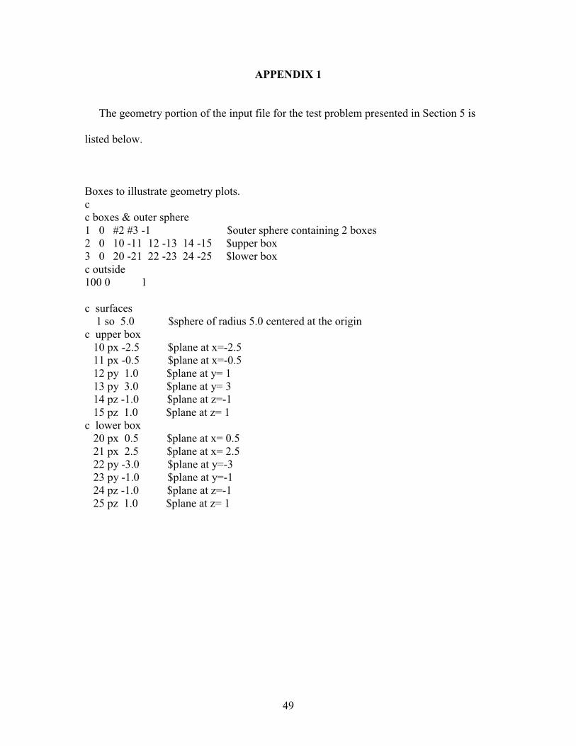
interactive geometry plotter. The model consists of a sphere containing two boxes. The
relevant geometry is listed in Appendix 1. Each plot shows the image in the plot plane at
z = 0 with extent 5 and with cell and surface labeling activated.
Figure 4 shows the plotted geometry for the correct model. The cell numbers are
labeled in red; the sphere is cell 1 and the boxes cells 2 and 3. The surface numbers are
labeled in black; the sphere is defined by surface 1, cell 2 by surfaces 10–13, and cell 3
by surfaces 20–23. For this model the geometry is well defined and all surfaces are
plotted using solid black lines.
38
Figure 4. Geometry plot for the correct model.
39
Figure 5 shows the plotted geometry for a faulty model. The error in this model was
created by omitting “#3” in the description of cell 1. The symbol # is the complement
operator which is used to designate not in.† Thus, cell 3 is specified, but cell 1 lacks the
information necessary to recognize its presence. Consequently, the surfaces for cell 3 are
plotted using dotted red lines. The plot legend signals the geometry error. The presence of
cell 1 inside of the sphere is unaffected, so it is plotted using solid black lines.
Figure 5. Geometry plot for error created by omitting #3 in the description of cell 1.
† The complement operator is just a shorthand cell-specification method that implicitly uses the intersection and union operator. Details describing the combinatorial geometry feature in MCNP are provided in the manual (Pelowitz, 2011).
40
Figure 6 contains the plotted geometry for a model in which surface 23 of cell 3
erroneously has been assigned a positive rather than a negative sense; i.e., +23 instead of
–23. This error causes the description of cell 3 to be incorrect which causes the
configuration of cell 3 to be incorrect. The three sides of cell 3 are plotted using solid
black lines. The upper boundary of cell 3 intersects the sphere and is plotted using a
dotted red line. The plot legend signals the geometry error. As with the previous model,
cell 1 is correctly specified and is plotted using solid black lines.
Figure 6. Geometry plot for error created by incorrectly specifying surface 23 of cell 3 with a positive sense.
41
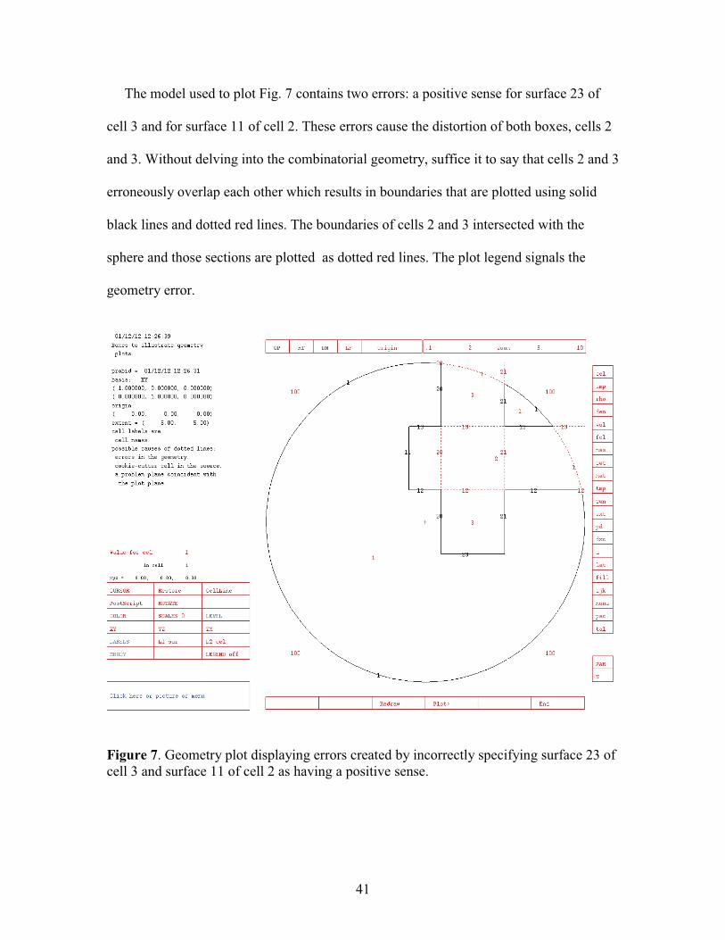
The model used to plot Fig. 7 contains two errors: a positive sense for surface 23 of
cell 3 and for surface 11 of cell 2. These errors cause the distortion of both boxes, cells 2
and 3. Without delving into the combinatorial geometry, suffice it to say that cells 2 and 3
erroneously overlap each other which results in boundaries that are plotted using solid
black lines and dotted red lines. The boundaries of cells 2 and 3 intersected with the
sphere and those sections are plotted as dotted red lines. The plot legend signals the
geometry error.
Figure 7. Geometry plot displaying errors created by incorrectly specifying surface 23 of cell 3 and surface 11 of cell 2 as having a positive sense.
42
For each of the models plotted in Figs. 4–7, MCNP uses a combination of Boolean
logic†
The POI of two lines in the plot plane is derived using the parametric form of a line as
given by Eq.(69). For line 1
and analytic geometry algorithms to determine and plot the geometry. These
algorithms create a geometry recognition capability that makes the geometry plotter a
powerful debugging tool for MCNP users. We do not delve into the Boolean logic aspect
of the geometry plotter in this article. However, next we do present some of the analytic-
geometry formulations that are used to determine the POI for curves in the plot plane.
These formulations have not been previously documented.
5.1. Intersection of two lines in the plot plane
1 2
4 5
s C C pt C C p% $% $
(110)
and line 2
1 2
4 5
s D D qt D D q% $% $
. (111)
These are lines through the points 0 1 4( , )P C C and 0 1 4( , )Q D D in the directions
2 5ˆ ˆA C i C j% $
!and 2 5
ˆ ˆB D i D j% $!
(Tierney, p. 438).
The POI is derived by equating s and t in Eqs.(110) and (111) so that
1 2 1 2
4 5 4 5
C C p D D qC C p D D q
$ % $$ % $
. (112)
Solving the second expression in Eq.(112) for q gives
† Boolean logic is also used for particle tracking.
43
4 5 4
5
C C p DqD
$ 0% . (113)
Substituting this result into the first expression in Eq.(112) and solving for p gives
" # " #5 1 5 2 4 4
2 5 2 5
D D C D C Dp
C D D C0 $ 0
%0
. (114)
The result in Eq.(114) is coded as “a” in inter.F line in.87 and is stored in the array
crs(nxp) as the location of the intersection of two lines.
Two vectors are parallel if their cross product is zero. Thus, here we calculate
2 5 2 5ˆ ˆA B C D D CF % 0 , (115)
which is the denominator of Eq.(114) and is coded as “b” in inter.F line in.85, can be
used as a check to assess whether the two lines intersect.
5.2. Intersection of a line and a quadratic in the plot plane
The POI of a line and a quadratic in the plot plane is derived using the parametric
form of a line as given by Eq.(69) and the equation of a general quadratic as given by
Eq.(32). For the line
1 2
4 5
s C C pt C C p% $% $
(116)
and the quadratic
2 222 23 33 12 13 112 2 2 0q s q st q t q s q t q$ $ $ $ $ % . (117)
44
Substitution of the expressions for s and t in Eq.(116) into Eq.(117), expanding, and
collecting terms in p gives
21 2 3 0c p c p c$ $ % , (118)
where
" #" #
2 21 23 2 5 22 2 33 5
2 12 2 13 5 23 1 5 2 4 22 1 2 33 4 5
2 23 11 12 1 13 4 23 1 4 22 1 33 4
22
2 .
c q C C q C q Cc q C q C q C C C C q C C q C C
c q q C q C q C C q C q C
% $ $
% $ $ $ $ $( ), -% $ $ $ $ $
(119)
Eq.(119) is coded in subroutine inter.F as in.97–in.101. The quadratic expression in
Eq.(118) is solved in subroutine quad.F. Real roots are used for POI plot analysis.
5.3. Intersection of two quadratics in the plot plane
The intersection of two quadratics in the plot plane makes use of Eq.(32) for both
equations. The POI formulation yields a quartic polynomial. The analysis for the roots of
a quartic has previously been developed (Cashwell and Everett, 1969) and the results are
coded in subroutine quart.F. Real roots are used for POI plotting.
6. Geometry plotter coding implementations
The MCNP geometry plotter contains nine primary subroutines. A discussion and
schematic of the code flow is presented in Appendix 2.
45
7. Summary and conclusions
The Los Alamos MCNP Monte Carlo code contains several useful features that were
developed in the late 1970s to create and plot geometry for radiation-transport models.
The MCNP geometry transformation capability permits the creation of objects using
simple analytic geometry expressions and object translation and/or rotation to locations
and/or orientations of interest in models. The geometry plotter provides 2-D images of
slices through model geometry.
Until now, detailed derivations of the expressions used by MCNP to perform
geometry transformations and geometry plots have not been available. Most of the
equations underlying the MCNP geometry transformation and geometry plot utility have
been derived here. Key expressions have been associated with lines of code in MCNPX
(MCNPX contains line identifiers whereas MCNP does not). The derived equations
agree with the expressions coded in MCNP.
The derivations indicate that the rotation-component “B” values in the TRF matrix are
transposed in MCNP relative to the theoretical representation. Coded expressions in
subroutines trfsrf.F, dunlev.F, etc. involving TRF matrix elements reflect this
discrepancy. MCNP corrects for this by transposing the TRF rotation elements in
subroutine trfmat.F during processing of the input data. Consequently, MCNP
transposes the TRF matrix twice in order to perform the correct coordinate-

46
transformation operation. It is unclear why this treatment was coded in MCNP. Future
work may be done to rewrite the code to simplify this treatment.
47
References
Breismeister J.F., ed., November 1993, “MCNP–A General Monte Carlo N–Particle
Transport Code, Version 4A,” Los Alamos National Laboratory report LA-12625-M, Ch.
2 pp. 159–161.
Brown F.B., ed., April 2003a, “MCNP–A General Monte Carlo N–Particle Transport
Code, Version 5, Volume I: Overview and Theory,” Los Alamos National Laboratory
report LA-CP-03-0245, Ch 2 pp. 182–185.
Brown F.B., ed., April 2003b, “MCNP–A General Monte Carlo N–Particle Transport
Code, Version 5, Volume II: User’ Guide,” Los Alamos National Laboratory report LA-
CP-03-0245, Ch 3 pp. 31–32.
Cashwell E.D. and Everett C.J., December 1969, “Intersection of a Ray with a Surface of
Third or Fourth Degree,” Los Alamos Scientific Laboratory report LA-4299.
Hsiung C.Y. and Mao G.Y., 1998, Linear Algebra, World Scientific, New Jersey, pp.
141–172.
Kwak J.H. and Hong S., 1997, Linear Algebra, Birkhauser, Boston, pp. 279–291.
Pelowitz D.B., ed., April 2011, “MCNPX User’s Manual Version 2.7.0,” Los Alamos
National Laboratory report LA-CP-11-00438.
Spain B., 2007, Analytical Conics, Dover Publications, Inc., Mineola, NY, pp. 66–70.
48
Thompson W.L., ed., November 1979, “MCNP–A General Monte Carlo Code for
Neutron and Photon Transport,” Los Alamos National Laboratory report LA-7396-M,
Revised, pp. 111–114.
Thompson W.L., Cashwell E.D., Godfrey T.N.K., Schrandt R.G., Deutsch O.L., and
Booth T.E., May 1980, “The Status of Monte Carlo at Los Alamos,” Los Alamos
National Laboratory report LA-8353-MS, pp. 17–22.
Thompson W.L., ed., November 1981, “MCNP–A General Monte Carlo Code for
Neutron and Photon Transport, Version 2B” Los Alamos National Laboratory report LA-
7396-M, Revised, p.1.
Tierney J.A., 1974, Calculus and Analytic Geometry, Allyn and Bacon, Inc., Boston, p.
226.
Trench W.F. and Kolman B., 1972, Multivariable Calculus with Linear Algebra and
Series, Academic Press, Inc., New York, pp. 222–223.
Wolfram S. (1991), Mathematica, Addison-Wesley, New York, Second Edition, pp. 121–
124.
Wylie C.R. (1975), Advanced Engineering Mathematics, McGraw-Hill, New York, pp.636–637.
49
APPENDIX 1
The geometry portion of the input file for the test problem presented in Section 5 is
listed below.
Boxes to illustrate geometry plots.cc boxes & outer sphere1 0 #2 #3 -1 $outer sphere containing 2 boxes2 0 10 -11 12 -13 14 -15 $upper box3 0 20 -21 22 -23 24 -25 $lower boxc outside100 0 1
c surfaces1 so 5.0 $sphere of radius 5.0 centered at the origin
c upper box10 px -2.5 $plane at x=-2.511 px -0.5 $plane at x=-0.512 py 1.0 $plane at y= 113 py 3.0 $plane at y= 314 pz -1.0 $plane at z=-115 pz 1.0 $plane at z= 1
c lower box20 px 0.5 $plane at x= 0.521 px 2.5 $plane at x= 2.522 py -3.0 $plane at y=-323 py -1.0 $plane at y=-124 pz -1.0 $plane at z=-125 pz 1.0 $plane at z= 1
50
APPENDIX 2
The MCNP geometry plotter makes use of nine primary subroutines. An overview of
these subroutines is provided here.†
As illustrated in Fig. 8, MCNP execution begins with the main.F, which controls
initialization, plotting, cross-section input, and particle transport. Subroutine imcn.F is
called by main.F to initiate transport. Subroutine imcn.F calls igeom.F where the
problem geometry is set up using subroutines mbody.F, trfsrf.F, and amatrx.F.
Subroutine mbody.F changes the macrobody representation of surface coefficients into
simple surfaces. Subroutine trfsrf.F is then used to perform any need transformations of
surfaces from local to global coordinates. Subroutine trfsrf.F uses amatrx.F to change
surface-coefficient representations from general quadratic to matrix form as discussed in
the material related to Eqs.(1)–(9). Following initialization, plotg.F is called for
geometry plotting.
† Original versions of several of these subroutines are identified in mcnp1a, release date August, 1977, as having been created by Charles A. Forest late in 1974 at Los Alamos Scientific Laboratory. Revisions to these subroutines have been made since mcnp1a.
51
AMATRXLoad the general-quadratic form of
the coefficients for each surfaceinto the AM matrix format.
MATMPYPerform matrix multiplication.
TRFSRFTransform the coefficients ofany surfaces that need it from
local to global coordinates.
MBODYExpand any macrobody surfaces
on cell cards to full surfaces.
IGEOMSet up the geometry.
IMCNInitiation for Monte Carlo transport.
PLOTGMake geometry plots.
MAINDriver for initialization, plotting,
cross-section input, and particle transport.
Figure 8. Initialization aspect of geometry plotting using MCNP. The primary subroutines used for geometry plotting are shown in the blue boxes.
Ash sown in Fig. 9, subroutine plotg.F calls two principal subroutines, amatrx.F and
viewz.F. Subroutine amatrx.F loads the general-quadratic form of the surface
coefficients for each surface into matrix form. At this point in execution, these
coefficients are the global-coordinate values GAM as given in Eq.(9).
Subroutine viewz.F is the driver routine for the calculation of the arcs and cell number
locations to be plotted. For each surface, viewz.F calls regula.F and pltsrf.F to calculate
the points that define the arcs used to plot each portion of each surface. Code flow for
these subroutines is shown in Fig. 9.
52
Subroutine regula.F calculates several quantities. First, the QM matrix coefficients
for each surface are calculated as discussed in the material related to Eqs.(25)–(32).
Second, the coefficients for the univariate equations in p are calculated for each arc. If the
QM coefficients are such that the equation is a straight line, the constants in Eq.(70) are
calculated directly. The diagonalization procedure discussed in the material related to
Eqs.(34)–(42) and Sections 4.2 and 4.3 is used for parallel or intersecting lines, a
parabola, ellipse, or hyperbola. For this procedure the diagonalization parameters D5 , 0s ,
and 0t parameters in Eqs.(45), (82), and (83) and the translation-rotation DIA in Eq.(36)
are calculated. The QM matrix is then formed using Eq.(39) to give the quadratic form
given of the curve in u,v in Eq.(43). The quadratic coefficients are evaluated to determine
whether the type of curve(s): parallel or intersecting lines, a parabola, ellipse, or
hyperbola. Finally, the coefficients for the univariate equations in p are calculated. For an
ellipse, circle, or point, the coefficients (square-root quantities) in Eq.(86) are used; for a
hyperbola the coefficients in Eq.(97) are used, and for a parabola the constants in
Eqs.(104) or (109) are used.
Subroutine pltsrf.F is the driver for the calculation of the points that define each of
the arcs of each surface in the plot plane. Points defining each are are loaded into a buffer
for plotting.
53
REGULACalculate the QM matrix and the
coefficients for the curves in p of eachsurface intersecting the plot plane.
PLTSRFDriver for calculation of the
points that define the arcs ofeach surface in the plot plane.
VIEWZCompute the arcs and cell-number
locations to be plotted.
AMATRXLoad the general-quadratic form of
the coefficients for each surfaceinto the AM matrix form.
PLOTGPlot the geometry.
Figure 9. MCNP upper-level geometry plotting subroutines.
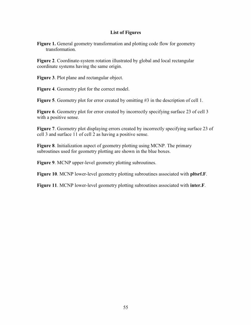
Figures 10 and 11 show the subroutines associated with pltsrf.F. Subroutine pltsrf.F
calls inter.F, ptost.F, and chkcel.F. Subroutine inter.F is used to find the intersections
within the plot window of each curve with all other curves. To do so, inter.F uses
sstop.F to determine the points where each curve (straight line, parabola, ellipse,
hyperbola) crosses the window boundary and regula.F. The POI for the intersection of
two lines, as given in Eq.(114), is calculated in inter.F. For the intersection of a line and
a general quadratic in the plot plane, subroutine inter.F calls quad.F to solve Eq.(118)
using Eq.(119) for one or two POIs. The intersection of two quadratics yields a quartic
polynomial that is solved using subroutine quart.F for the POIs.
Subroutine ptost.F calculates the point ( ), ( )s p t p from the parametric representation
of each curve in the plot plane. Expressions for a straight line, parabola, ellipse, and
hyperbola are given in Eqs.(69)–(70), (103)–(104), (88)–(89), and (96)–(97),
respectively.
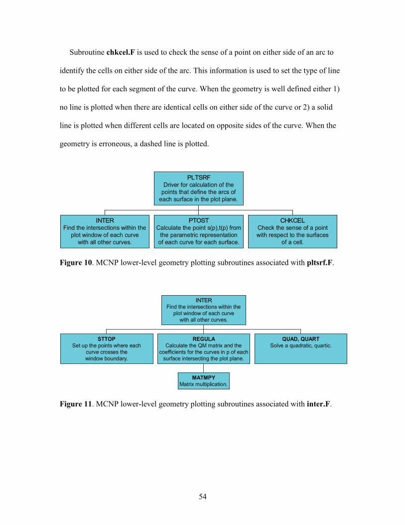
54
Subroutine chkcel.F is used to check the sense of a point on either side of an arc to
identify the cells on either side of the arc. This information is used to set the type of line
to be plotted for each segment of the curve. When the geometry is well defined either 1)
no line is plotted when there are identical cells on either side of the curve or 2) a solid
line is plotted when different cells are located on opposite sides of the curve. When the
geometry is erroneous, a dashed line is plotted.
INTERFind the intersections within the
plot window of each curvewith all other curves.
PTOSTCalculate the point s(p),t(p) from
the parametric representationof each curve for each surface.
CHKCELCheck the sense of a pointwith respect to the surfaces
of a cell.
PLTSRFDriver for calculation of the
points that define the arcs ofeach surface in the plot plane.
Figure 10. MCNP lower-level geometry plotting subroutines associated with pltsrf.F.
STTOPSet up the points where each
curve crosses thewindow boundary.
MATMPYMatrix multiplication.
REGULACalculate the QM matrix and the
coefficients for the curves in p of eachsurface intersecting the plot plane.
QUAD, QUARTSolve a quadratic, quartic.
INTERFind the intersections within the
plot window of each curvewith all other curves.
Figure 11. MCNP lower-level geometry plotting subroutines associated with inter.F.
55
List of Figures
Figure 1. General geometry transformation and plotting code flow for geometry transformation.
Figure 2. Coordinate-system rotation illustrated by global and local rectangular coordinate systems having the same origin.
Figure 3. Plot plane and rectangular object.
Figure 4. Geometry plot for the correct model.
Figure 5. Geometry plot for error created by omitting #3 in the description of cell 1.
Figure 6. Geometry plot for error created by incorrectly specifying surface 23 of cell 3 with a positive sense.
Figure 7. Geometry plot displaying errors created by incorrectly specifying surface 23 of cell 3 and surface 11 of cell 2 as having a positive sense.
Figure 8. Initialization aspect of geometry plotting using MCNP. The primary subroutines used for geometry plotting are shown in the blue boxes.
Figure 9. MCNP upper-level geometry plotting subroutines.
Figure 10. MCNP lower-level geometry plotting subroutines associated with pltsrf.F.
Figure 11. MCNP lower-level geometry plotting subroutines associated with inter.F.

56
List of Tables
None.