Linear-Time Reconstruction of Zero-Recombinant Mendelian Inheritance on Pedigrees without Mating Loops

Authors:

Lan Liu, Tao Jiang

Univ. California, Riverside USA

,

Outline

Introduction and problem definition The linear system for ZRHC A linear-time algorithm for Loop-free

ZRHC Conclusion

Pedigree

Camilla, Duchess of Cornwall

Peter Phillips Zara Phillips

Diana,Princess of Wales

Prince Williamof Wales

Prince Henry ofWales

PrincessBeatrice of York

PrincessEugenie of York

Lady LouiseWindsor

Prince Charles,Prince of Wales

Princess Anne, Princess Royal

CommanderTimothy Laurence

Prince Andrew,Duke of York

SarahMargaret Ferguson

Prince Edward, Earl of Wessex

Sophie Rhys-Jones

Elizabeth II ofthe United Kingdom

Prince Philip,Duke of Edinburgh

CaptainMark Phillips

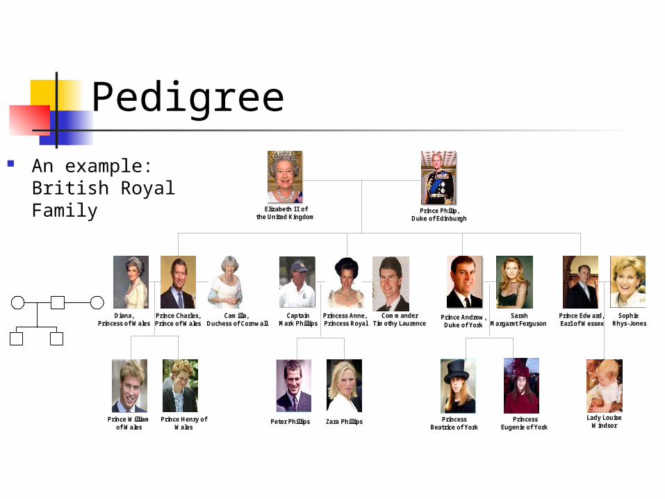
An example: British Royal Family

Biological Background

2 2

2 1

1 2

1 1

1 2

Genotype

Haplotype

Locus

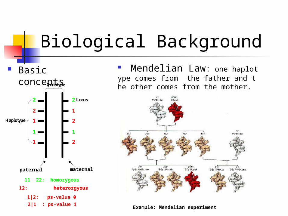
Basic concepts Mendelian Law: one haplotype comes from the father and the other comes from the mother.

Example: Mendelian experiment

paternal maternal

12: heterozgyous11 22: homozygous

2|1 : ps-value 1 1|2: ps-value 0

Notations and Recombinant

1122

2222

Genotype

1222

2122

Haplotype Configuration

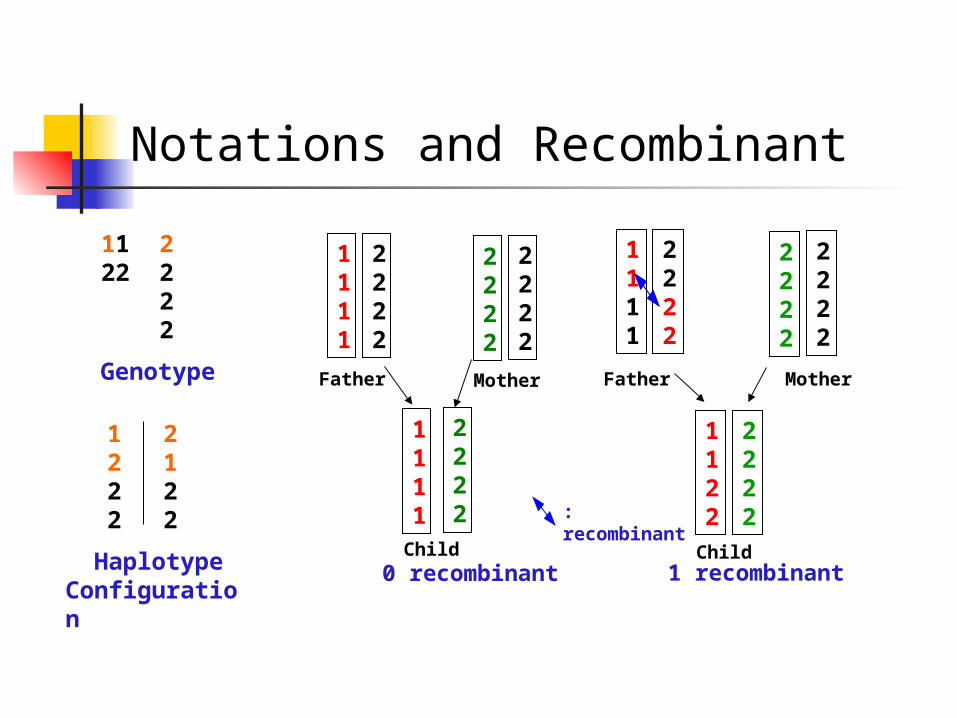
0 recombinant

1111

2222

2222

2222

1111

2222

MotherFather

Child

: recombinant

1111

2222

2222

2222

1122

2222

1 recombinant

MotherFather

Child

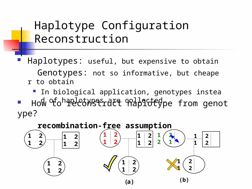
Haplotype Configuration Reconstruction

Haplotypes: useful, but expensive to obtain Genotypes: not so informative, but cheaper to obtain

In biological application, genotypes instead of haplotypes are collected.

How to reconstruct haplotype from genotype? recombination-free assumption

1 21 2

1 22 1

1 21 2

(b)

1 21 2

1 21 2

1 21 2

1 21 2

1 21 2

1 21 2

(a)

The Loop-free ZRHC problem

Problem definition Given a loop-free pedigree and the genotype infor

mation for each member, find a recombination-free haplotype configuration for each member that obeys the Mendelian law of inheritance.

Solutions to the ZRHC problem

A particular solution: any numerical assignment

A general solution: the span of a basis in the solution space to its associated homogeneous system, offset from the origin by a vector, namely by any particular solution.

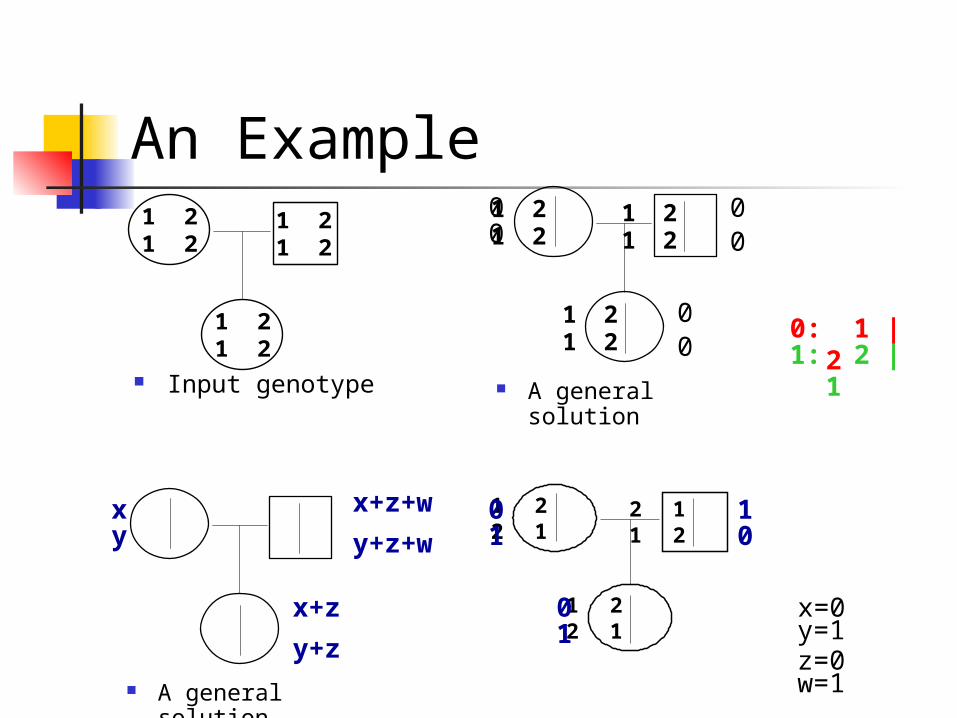
An Example0 1 2

1 21 21 2

1 21 2 0: 1 | 2

1: 2 | 1

00

00

0

A general solution

2 11 2

1 22 1

1 22 1

x

x+z

y+z

yx+z+w

y+z+w01

01

10

x=0y=1z=0w=

1 A general

solution

1 21 2

1 21 2

1 21 2

Input genotype

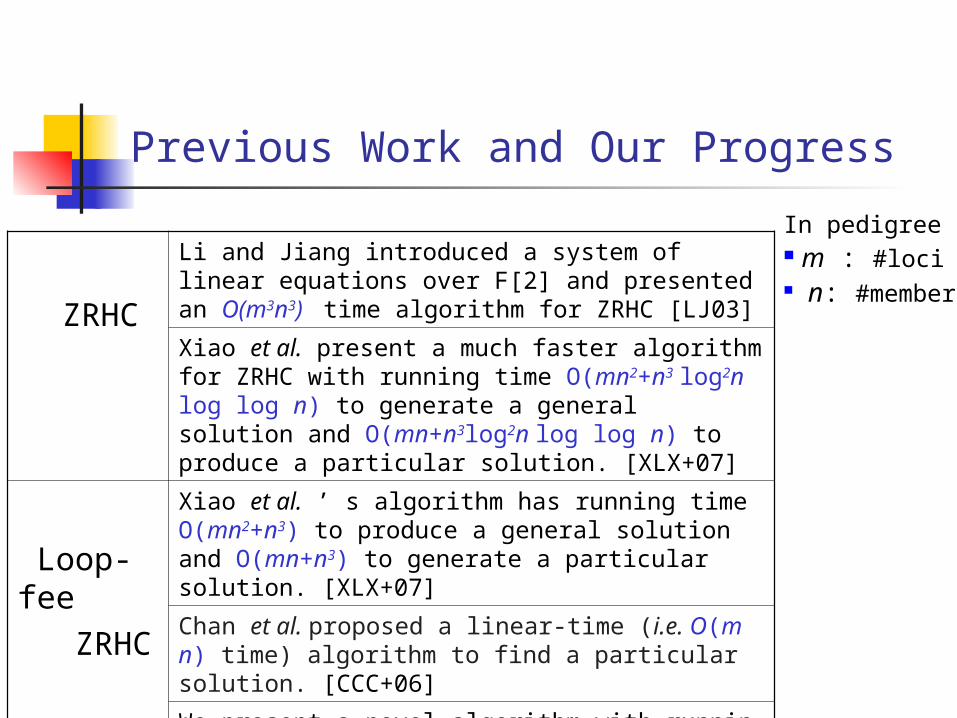
Previous Work and Our Progress

ZRHC

Li and Jiang introduced a system of linear equations over F[2] and presented an O(m3n3) time algorithm for ZRHC [LJ03]

Xiao et al. present a much faster algorithm for ZRHC with running time O(mn2+n3 log2n log log n) to generate a general solution and O(mn+n3log2n log log n) to produce a particular solution. [XLX+07]

Loop-fee ZRHC

Xiao et al. ’ s algorithm has running time O(mn2+n3) to produce a general solution and O(mn+n3) to generate a particular solution. [XLX+07]

Chan et al. proposed a linear-time (i.e. O(mn) time) algorithm to find a particular solution. [CCC+06]We present a novel algorithm with running time O(mn2) to produce a general solution and O(mn) to generate a particular solution.

In pedigree m : #loci n: #members

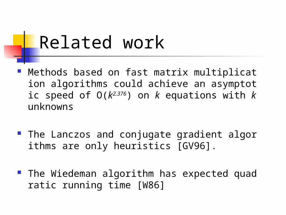
Related work Methods based on fast matrix multiplication algorith

ms could achieve an asymptotic speed of O(k2.376) on k equations with k unknowns

The Lanczos and conjugate gradient algorithms are only heuristics [GV96].

The Wiedeman algorithm has expected quadratic running time [W86]

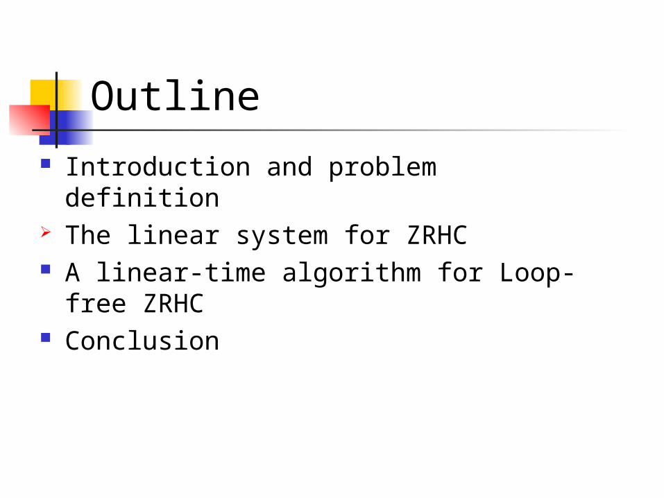
Outline Introduction and problem definition The linear system for ZRHC A linear-time algorithm for Loop-free

ZRHC Conclusion

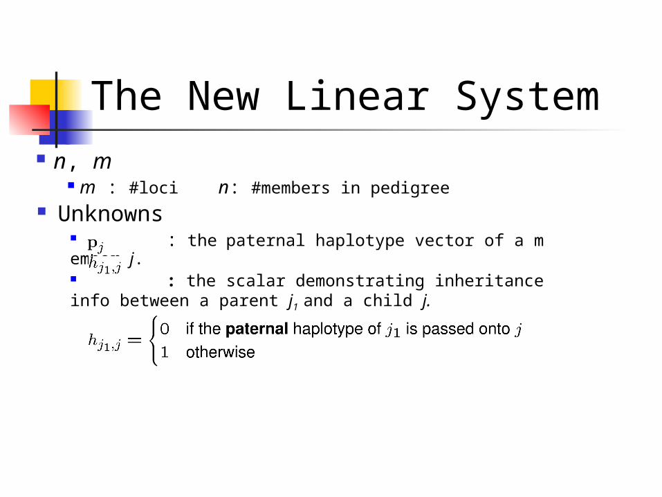
The New Linear System n, m

m : #loci n: #members in pedigree Unknowns

: the paternal haplotype vector of a member j. : the scalar demonstrating inheritance info between a parent j1 and a child j.

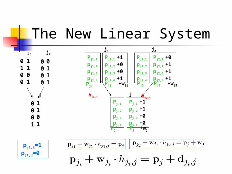
The New Linear System

0100

1101

0000

0111

0 0 0 1

1101

j2 j1

j

Pj1,1

pj1,2

pj1,3

pj1,4

j2

j

j1

Pj2,1

pj2,2

pj2,3

pj2,4

Pj2,1 +0

pj2,2 +1

pj2,3 +1

pj2,4 +1

Pj,1

pj,2

pj,3

pj,4

Pj,1 +1

pj,2 +1

pj,3 +0

pj,4 +0

hj1,j hj2,j

Pj1 +wj1Pj1 Pj2 Pj2 +wj2

Pj1,1 +1

pj1,2 +0

pj1,3 +0

pj1,4 +1

Pj Pj +wj

pj1,2=1 pj1,

3=0

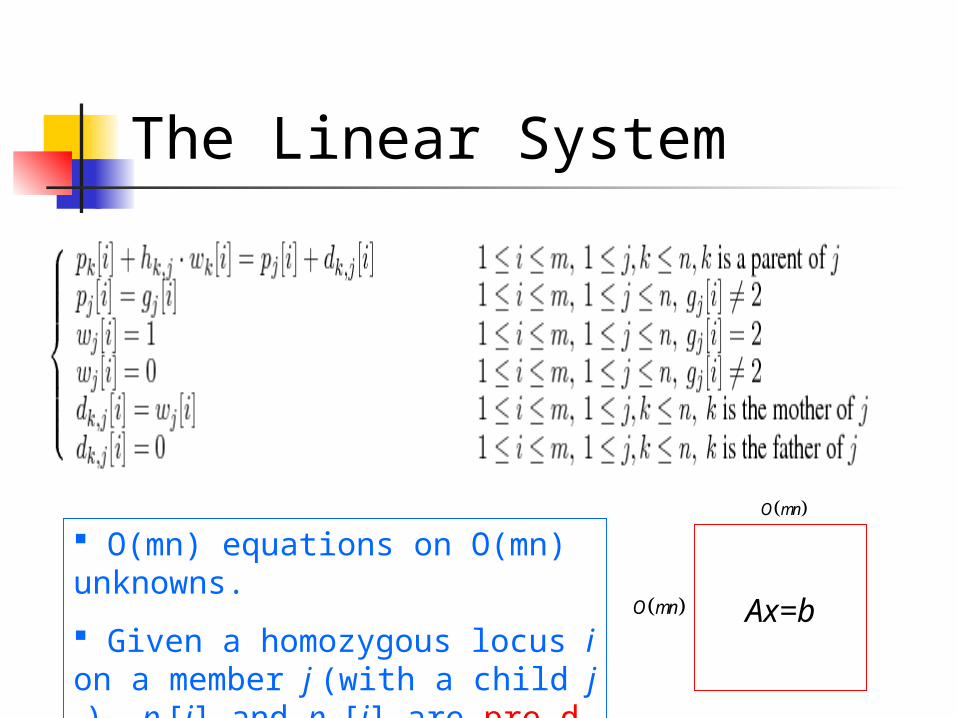
The Linear System

O(mn) equations on O(mn) unknowns.

Given a homozygous locus i on a member j (with a child j1), pj[i] and pj1[i] are pre-determined.

O mn

O mn Ax=b

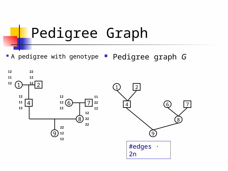
Pedigree Graph A pedigree with genotype

1

6

9

8

2

4 7

12

11

12

12

11

12

22

12

12

12

22

22

12

12

12

11

22

12

22

12

12

1

6

9

8

2

4 7

Pedigree graph G

#edges · 2n

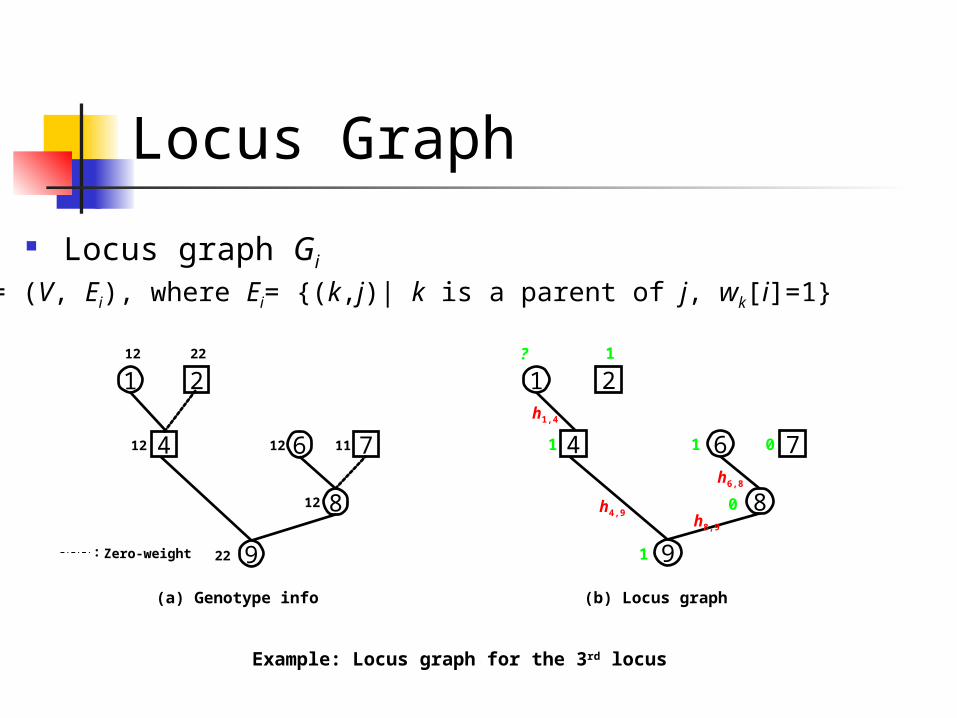
Locus Graph

Locus graph Gi

1

6

9

8

2

4 7

12 22

12 12 11

12

22

Example: Locus graph for the 3rd locus

Gi = (V, Ei), where Ei= {(k,j)| k is a parent of j, wk[i]=1}

(a) Genotype info

Zero-weight

:

1

6

9

8

2

4 7

? 1

1 1 0

1

0

h1,4

h4,9h8,9

h6,8

(b) Locus graph

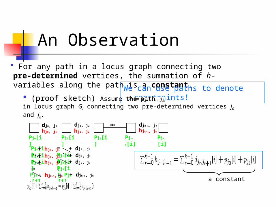
An Observation For any path in a locus graph connecting two pre-determined vertices, the summation of h-variables along the path is a constant. We can use paths to denote

constraints!

a constant

+ dj0, j1

…

Pj1[i]hj1, j2

Pj2[i] Pjk-1[i] Pjk[i]hjk-1, jk

dj1, j2 djk-1, jk

Pj1[i] + dj1, j2+ hj1, j2 = Pj2[i]Pj2[i] + dj2, j3+ hj2, j2 = Pj3[i]…

Pjk-1[i] + djk-1, jk+ hjk-1, jk= Pjk

[i]

Pj0[i]hj0, j1

dj0, j1

Pj0[i] = Pj1[i]

+ hj0, j1

(proof sketch) Assume the path in locus graph Gi connecting two pre-determined vertices j0 and jk .

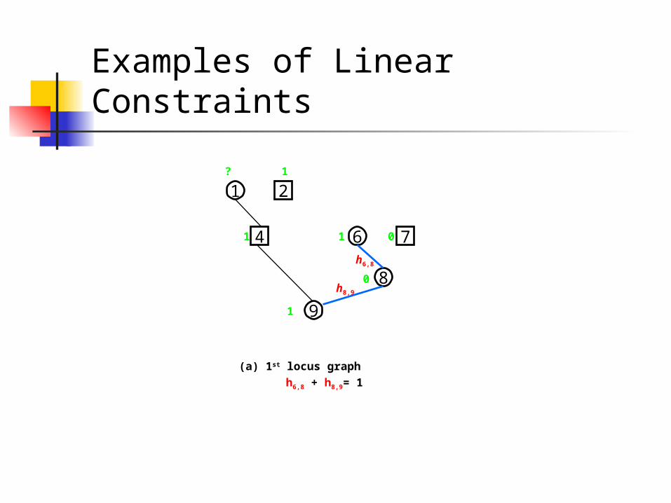
Examples of Linear Constraints

1

6

9

8

2

4 7

? 1

1 1 0

1

0h8,9

h6,8

(a) 1st locus graph h6,8 + h8,9= 1

Linear Constraints

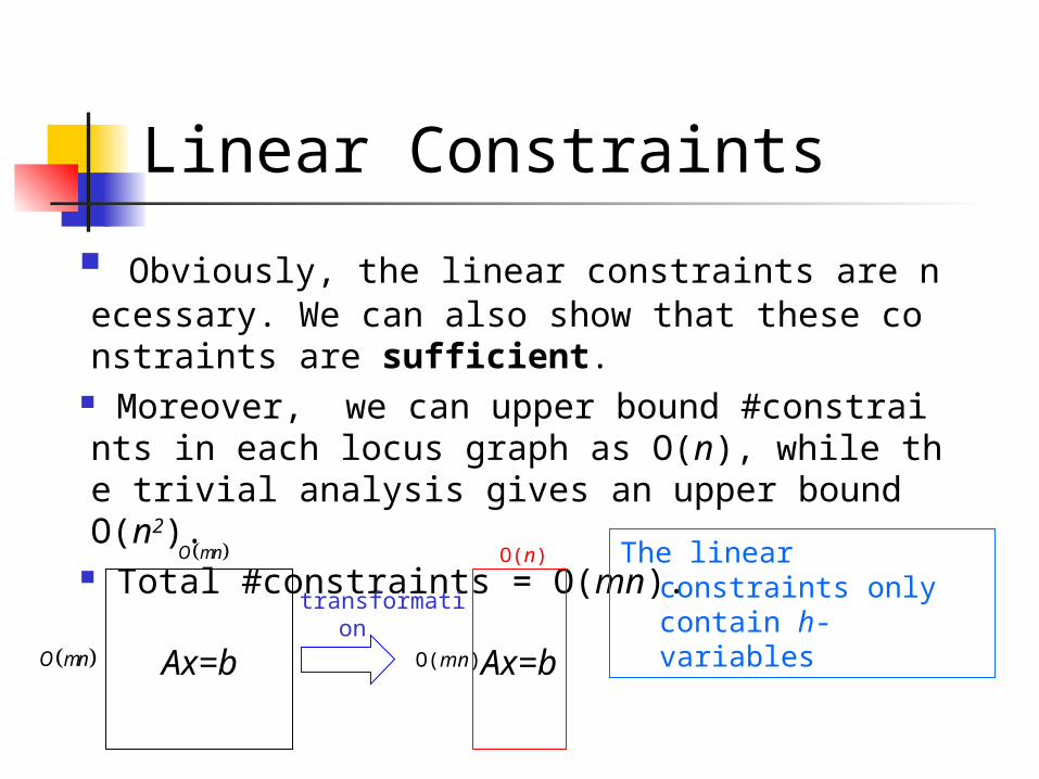
Obviously, the linear constraints are necessary. We can also show that these constraints are sufficient.

Moreover, we can upper bound #constraints in each locus graph as O(n), while the trivial analysis gives an upper bound O(n2).

Total #constraints = O(mn).

Ax=b

O mn

O mn Ax=b

transformation

O(mn)

O(n) The linear constraints only contain h-variables

Outline Introduction and problem definition The linear equations for ZRHC A linear-time algorithm for ZRHC Conclusion

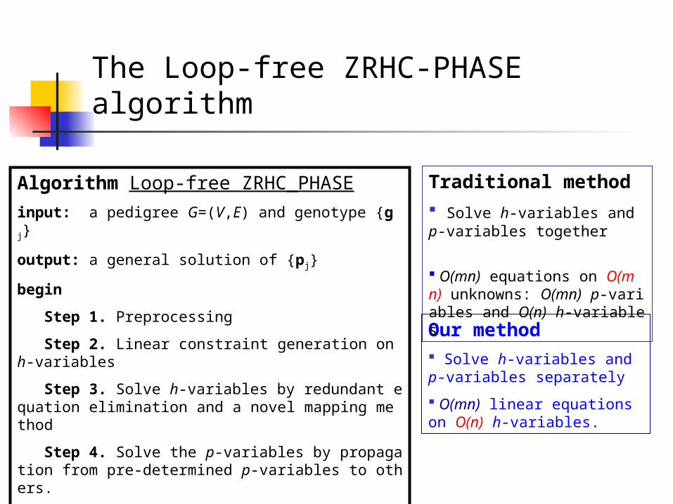
The Loop-free ZRHC-PHASE algorithm

Algorithm Loop-free ZRHC_PHASEinput: a pedigree G=(V,E) and genotype {gj}

output: a general solution of {pj}

begin

Step 1. Preprocessing

Step 2. Linear constraint generation on h-variables

Step 3. Solve h-variables by redundant equation elimination and a novel mapping method

Step 4. Solve the p-variables by propagation from pre-determined p-variables to others.

end

Our method Solve h-variables and p-variables separately O(mn) linear equations on O(n) h-variables.

Traditional method Solve h-variables and p-variables together O(mn) equations on O(mn) unknowns: O(mn) p-variables and O(n) h-variables.

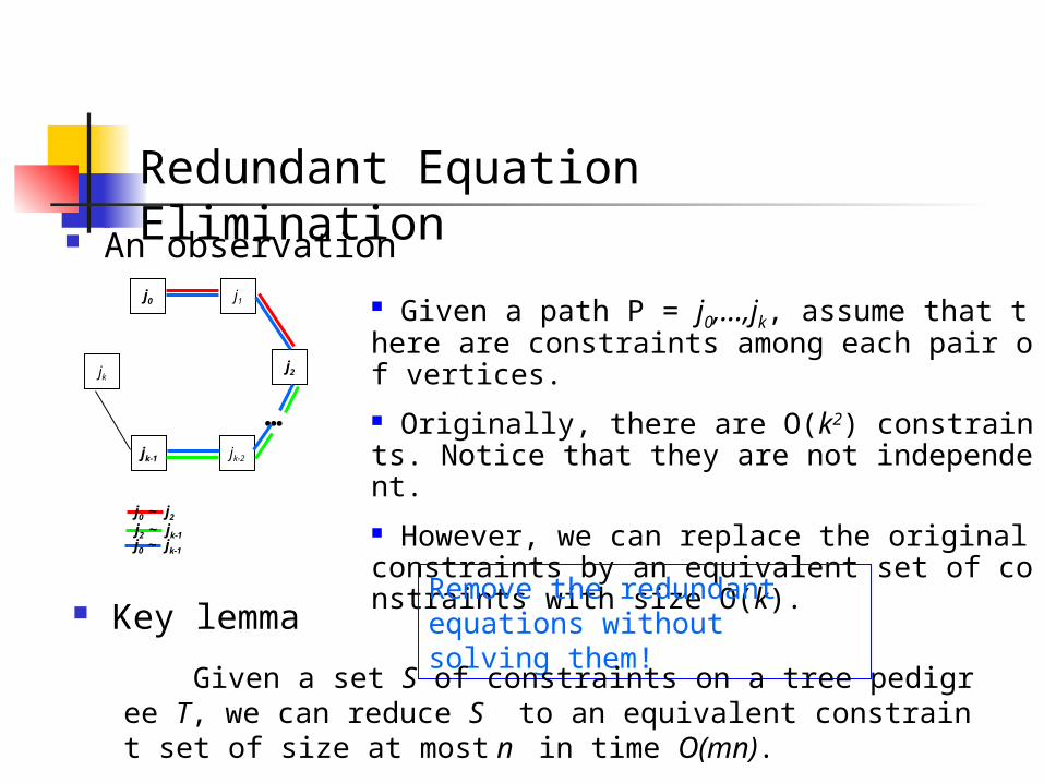
Redundant Equation Eliminationj0 j1

jk-1

jk

jk-2

j2

…

An observation

Given a path P = j0,…,jk, assume that there are constraints among each pair of vertices. Originally, there are O(k2) constraints. Notice that they are not independent. However, we can replace the original constraints by an equivalent set of constraints with size O(k).j2 ~ jk-1

j0 ~ j2

j0 ~ jk-1

Remove the redundant equations without solving them!

Key lemma

Given a set S of constraints on a tree pedigree T, we can reduce S to an equivalent constraint set of size at most n in time O(mn).

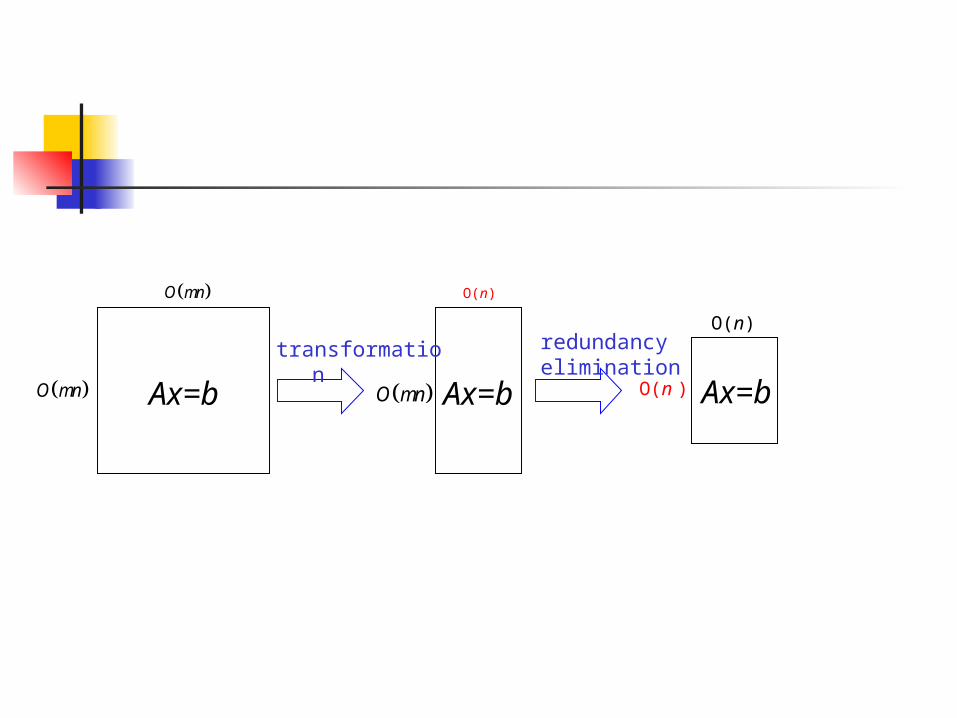
Ax=b

O mn

O mn Ax=b O mn Ax=b

transformation

redundancy elimination

O(n )

O(n)

O(n)

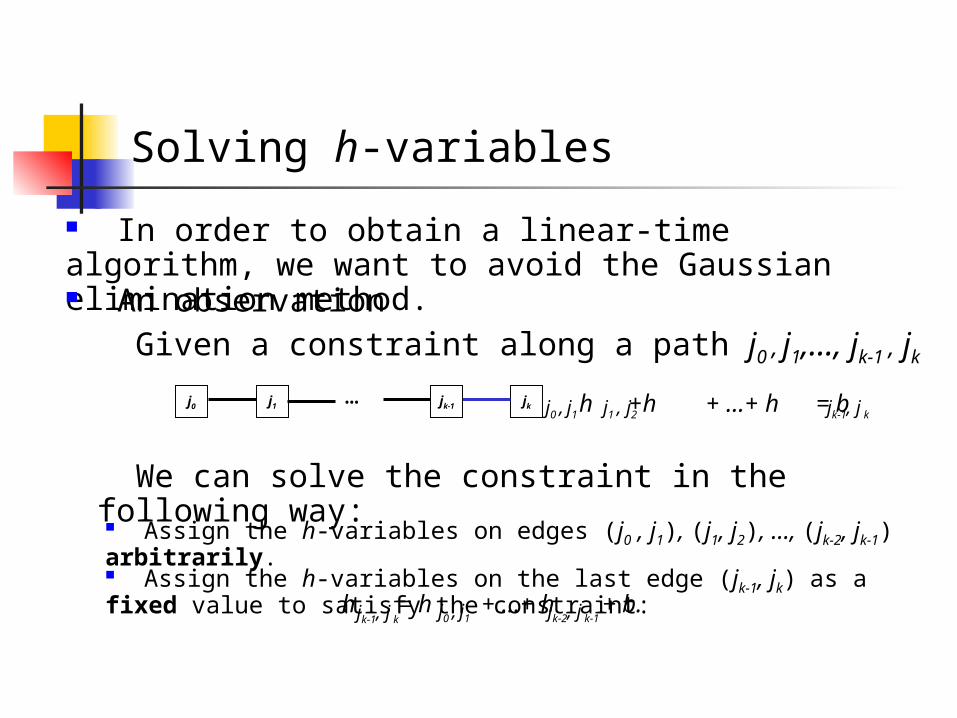
Solving h-variables

In order to obtain a linear-time algorithm, we want to avoid the Gaussian elimination method.

j0 j1 jk… jk-1

An observation Given a constraint along a path j0 , j1,…, jk-1 , jk

h +h + …+ h = b j0 , j1 j1 , j2 jk-1, j k

Assign the h-variables on edges (j0 , j1), (j1, j2), …, (jk-2, jk-1) arbitrarily. Assign the h-variables on the last edge (jk-1, jk) as a fixed value to satisfy the constraint: h = h + …+ h + b.j0 , j1 jk-2, j k-1jk-1, j k

We can solve the constraint in the following way:

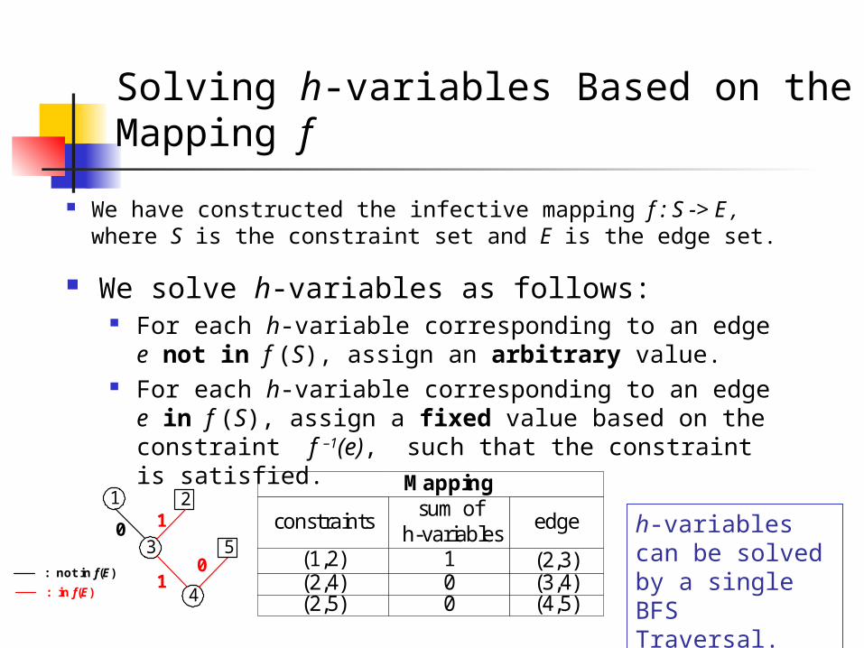
Solving h-variables Based on the Mapping f

We have constructed the infective mapping f : S -> E , where S is the constraint set and E is the edge set.

h-variables can be solved by a single BFS Traversal.

1 2

3

4

5constraints

(1,2)

edge

(2,3)(2,4) (3,4)(2,5) (4,5)

Mappingsum of

h-variables100

0 1

10: not in f(E)

: in f(E)

We solve h-variables as follows: For each h-variable corresponding to an edge e not

in f (S), assign an arbitrary value. For each h-variable corresponding to an edge e in f

(S), assign a fixed value based on the constraint f –

1(e), such that the constraint is satisfied.

Conclusion We present an efficient algorithm for Loop-fee ZRH

C with running time O(mn) to generate a particular solution and O(mn2) to generate a general solution .

Thanks for your time and attention!