Life cycle implications of product modular architectures in closed-loop supply chains

ORIGINAL ARTICLE

Life cycle implications of product modular architecturesin closed-loop supply chains

Wu-Hsun Chung & Gül E. Okudan Kremer &

Richard A. Wysk

Received: 6 June 2013 /Accepted: 4 October 2013 /Published online: 10 November 2013# Springer-Verlag London 2013

Abstract Most of the product life cycle costs and environ-mental impacts are determined during product design stage. Aproduct supply chain network can be seen as a system dealingwith product life cycle processes. Ideally, a product should bedesigned to have a structure yielding a good life cycle perfor-mance in its existing supply chain network. However, there isa lack of research related to modeling supply chain effects inthe product design stage. This paper aims at investigating thesupply chain effects on product modular design. The life cycleperformance of a modular structure (life cycle cost and lifecycle environmental impact) at various supply chain states isevaluated by a supply chain evaluationmodel and analyzed bystatistical techniques. The preliminary results indicate that thesupply chain-related effects on product life cycle performanceare significant and modular structure optimization is effectivein reducing the surge of life cycle cost and life cycle environ-mental impact caused by various supply chain states. Themain supply chain effects are identified for use in productdesign improvement.

Keywords Design for life cycle . Design for logistics .

Modular design . Closed-loop supply chains

1 Introduction

Product development is a creative process that realizes poten-tial market demands into a specific product. Traditionally,product manufacturing and service have been the chief con-siderations during product development. Due to growing en-vironmental concerns in the past decades, product reuse andrecycling at product retirement stage also garnered attentionfrom researchers. Nowadays, the design philosophy consider-ing a product from its birth to death, design for life cycle(DFLC), is a common approach. According to prior studies,most of the product life cycle costs (LCC) and environmentalimpacts (LCEI) are determined at the product design stage [5,6, 13]. Decisions in product design affect product LCC andLCEI profoundly; for example, modular design is known as acommon technique to reduce a product’s LCC and LCEI. Themodular architecture is able to influence manufacturing costs(e.g., assembly), ease of service (e.g., disassembly and reas-sembly), and effort to retire the product [16]. Its concept is toseparate a product into functional or logical groups of com-ponents (modules).

Supply Chain Council [19] defined a supply chain as“every effort involved in producing and delivering a finalproduct or service , from the supplier’s supplier to the cus-tomer’s customer.” A product’s supply chain network per-forms the product’s life cycle processes from birth to death.Product design and its supply chain have an inseparablerelationship. Prior relevant research has revealed that designdecisions in product architecture impact the life cycle perfor-mance of supply chains [12, 22]. There is also a significantdifference in supply chain performance (in terms of time andcost) between considering and not considering supply chainduring product design stage [3]. Thus, product design deci-sions coupled with supply chain factors are critical and shouldbe integrated. Designing logistic-friendly products for a sup-ply chain to minimize product LCC and LCEI is an important

W.<H. Chung :G. E. Okudan KremerDepartment of Industrial and Manufacturing Engineering,Pennsylvania State University, University Park, PA 16802, USA

G. E. Okudan Kremer (*)School of Engineering Design, Pennsylvania State University,University Park, PA 16802, USAe-mail: [email protected]

R. A. WyskDepartment of Industrial and System Engineering, North CarolinaState University, Raleigh, NC 27695, USA

Int J Adv Manuf Technol (2014) 70:2013–2028DOI 10.1007/s00170-013-5409-8

issue. However, the research in the area of modeling supplychain effects in the product development phase is insufficient[2].

This paper is investigating the supply chain effects onproduct design, particularly on product modular structures.The life cycle performance of a modular structure at varioussupply chain states is evaluated by a supply chain optimizationmodel and analyzed by statistical techniques. Three criteria,namely (1) LCC, (2) life cycle environmental energy consump-tion (LCEC), and (3) their aggregation (LCC&LCEC), are usedto measure the life cycle performance. The main effects of thesupply chain are identified and discussed. More importantly,this paper reveals the potential of modular structures to improveproduct life cycle performance at various supply chain states.

The remainder of this paper includes four additional sec-tions. Section 2 reviews the relevant literature regarding mod-ular architectures and the importance of matching productarchitecture design with supply chains. Section 3 describesthe case for analysis and Section 4 shows analysis results.Section 5 concludes based on the findings of this paper andpresents directions for future work.

2 Literature review

Because of environment protection legislations such as Euro-pean product take-back policy, a product’s entire life needs tobe fully considered during product design stage. Productarchitecture design involves how to arrange product compo-nents spatially and logically. Newcomb et al. [16] asserted thata product’s architecture, determined during configuration de-sign stage, plays an important role in determining its life cyclecharacteristics and applied modular architectures into productdesign for life cycle objectives (e.g., service, recycling, reuse).This section outlines the evolution of product modularity andthen discusses the pros and cons of matching a product’sarchitecture design with its supply chain.

2.1 Product modular architectures

Allen and Calson-Skalak [1] stated that a module is a compo-nent or group of components that can be taken off from theproduct non-destructively as a unit and have a unique basicfunction necessary for the product to operate as desired. Ulrichand Eppinger [20] noted that a modular architecture is one inwhich each functional element of the product is implementedby exactly one chunk (module) and in which there are fewinteractions between chunks; such a modular architectureallows a design change to be made to one chunk withoutaffecting the others.

A relevant term, modularity is the degree to which a prod-uct’s architecture is composed of modules with minimal in-teractions between modules [7]. Ulrich and Tung [21] defined

it in terms of two characteristics of product design: “(1) Simi-larity between the physical and functional architecture of thedesign and (2) Minimization of incidental interactions betweenphysical components.” In the past, although some researchersalready began investigating modular design for life cycle (e.g.,[16]), product functionality has been the predominant focus inmodular design. Product architecture is seen as the arrangementof functional elements of a product into physical blocks.Pimmler and Eppinger [17] defined component interactionsinto four functional forms: spatial, energy, information, andmaterial; and then clustered the components into functionalmodules based on these interactions.

With growing environmental consciousness, more andmore common life cycle characteristics are integrated intomodular design. Newcomb et al. [16] defined the relationshipsbetween components as life cycle issues (e.g., recycling, post-life intent, and service frequency) and then incorporated theminto a modularity measure. Gu and Sosale [8] defined thecomponent relationship for functionality (physical contact,energy, material, signal, and force exchanges) and also iden-tified life cycle characteristics (assemblability, serviceability,recyclability); they combined these into a modularity measurethen used simulated annealing to cluster the components intoproduct modules. Likewise, Sand et al. [18] analyzed andaligned the functional structure, physical architecture, and lifecycle characteristics of a product in various matrices, and then

Supp

ly C

hain New Re-engineering Breakthrough

Exi

stin

g

Continuous

improvementDesign for Logistics

Existing New

Product

Fig. 1 A framework for product and supply chain decision making(source: [2])

Product dataProduct modular structure forevaluation

Supply chain (SC) optimization model for product modular structure evaluation

Life cycle energy performance of the optimized product modular structure at various supply chain states

Conclusions

Data of various supply chain states

Statistical analysis and comparisons

Life cycle cost performance of the evaluated product modular structure at various supply chain states

Fig. 2 Analysis flow

2014 Int J Adv Manuf Technol (2014) 70:2013–2028

aggregated these into an enhanced modular information ma-trix. A clustering modular group algorithm was invented tomodularize the product based on the matrix. Umeda et al. [23]defined the interaction in component similarity based on theattributes of product components, constituent materials, phys-ical lifetime, and value lifetime for four life cycle options:recycling, maintenance, reuse, and updating. A clusteringtechnique, self-organizing maps, was adopted to generateproduct modules. Although the application of modular designhas been expanded from functionality to life cycle character-istics, the scope for product structure evaluation is still limitedto a product itself and does not consider the existing supplychain network for the product. Whether the product fits in theexisting supply chain during the product life cycle and hasgood life cycle performance is ignored.

2.2 Matching product architecture design with supply chains

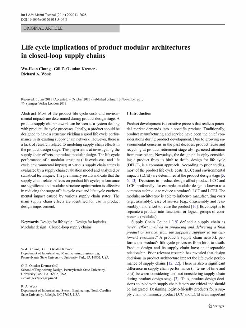
A product supply chain can be seen as a support system toprocess a product across the product life cycle, and the productand its supply chain need to fit each other well so that theoverall operation performance can be optimized. When de-signing either one, one should consider the characteristics ofthe other. As shown in Fig. 1, Appelqvist et al. [2] proposed aframework in which both product and supply chain designsare categorized as existing or new. The four categories in theframework are described below.

& Breakthrough is the most challenging situation where anew product is being designed and simultaneously, a newsupply chain for the product is being designed also.

& Design for logistics (DFL) indicates that when a newproduct is introduced to an existing supply chain, it shouldbe designed adapting to it.

& Re-engineering here represents the situation that the sup-ply chain is changed without affecting product structures.

& Continuous improvement focuses on doing the samethings in a more efficient way without affecting theexisting product and supply chain structures.

Appelqvist et al. [2] noted that breakthrough and DFL arethe areas that limited papers in the literature only discuss. The

Table 1 Attributes of the components in the refrigerator (source: [22])

No. Component Material Weight (g) Price ($) Mfg. cost ($) Mfg. energy (kWh) MTBF (month) End-of-life option Service intent

1 Cabinet frame Fe 23,606 180 53.13 72.9 312 RU/RC/D N

2 Cabinet Plastic 29,313 788 243.13 147.7 192 RC/D N

3 Duct Plastic 1,028 40 12.65 5.2 162 RC/D N

4 Fan unit1 Fe 483 26 8.51 1.5 108 RC/D Y

5 Fan unit2 Fe 483 26 8.51 1.5 108 RC/D Y

6 Evaporator Al 532 50 14.01 1.6 120 RU/RC/D N

7 Rear board Fe 986 27 8.67 3.0 336 RU/RC/D N

8 Compressor Fe 7,985 80 24.01 24.7 144 RU/RC/D N

9 Condenser Fe 2,669 40 12.44 8.2 204 RU/RC/D N

10 Base Fe 1,240 26 8.25 3.8 324 RU/RC/D N

11 Door1 Fe 2,693 60 19.10 8.3 336 RU/RC/D N

12 Door2 Fe 4,331 70 21.88 13.3 348 RU/RC/D N

13 Gasket1 Plastic 40 6 2 0.2 72 RC/D Y

14 Gasket2 Plastic 60 9 3 0.3 72 RC/D Y

15 Door liner1 Plastic 2,236 52 16 11 168 RC/D N

16 Door liner2 Plastic 4,472 104 32 22 168 RC/D N

17 Control unit Fe/Plastic 4,677 332 108.08 16.8 156 RU/RC/D N

18 Heater Al 112 42 13.44 0.4 84 RC/D Y

19 Dryer Cu 111 13 3.96 0.3 144 RU/RC/D N

20 Shelf set Plastic 1,266 34 10.5 6.4 252 RC/D N

RU reuse, RC recycle, D dispose

Product LevelProduct

1 2 3

2 31 4 75 6

Module Level

Component Level

Fig. 3 Product hierarchical architecture

Int J Adv Manuf Technol (2014) 70:2013–2028 2015

research in this paper is targeting the latter, DFL, designing anew product for an existing supply chain.

Under DFL, researchers have studied how to improve theoverall life cycle performance of supply chains through thechange of product modular structures. Umeda et al. [22]developed a life cycle simulation model based on an existingproduct process network to find an optimal product modularstructure and used LCC and LCEI in the network as

modularity measures. Kwak and Kim [12] formulated theexisting recovery supply chain network of a product (cellphone) as a mixed integer linear programming (MILP) modelto evaluate product structures and to determine which productstructure can maximize the product recovery profit. Theirwork successfully linked product design to product recoverysupply chains and showed how different designs affect end-of-life recovery in the supply chains.

Krikke et al. [10] formulated the closed-loop supply chainof a product (refrigerator) also as a MILP model for productstructure evaluation and concluded that the modular structureadvocating sustainability dominates the other structures over-all in synergy between supply cost, energy use, and waste.

In summary, the studies aforementioned all assume thestatic state of the existing supply chain to determine productstructure during product design stage; the input parameters ofthe supply chain models in these studies are all deterministic.However, the dynamic state of the existing supply chain mayoccur in practice. Some parameters of the supply chain modelsare variable during a product’s life cycle. For instance, during

Demand Locations

Assembly Facilities

Component Suppliers

F1

F2

F3

S1

S2

S3

C2

C1D2

D1

F11

F10

F9

F8

F7

F6

Disassembly Facilities

Disposal Facilities

Recycling Facilities

Rebuild FacilitiesForward Logistics (Pull)

Reverse Logistics (Push)

F5

F4

Service Facilities

Fig. 4 Closed-loop supply chainnetwork for the refrigerator

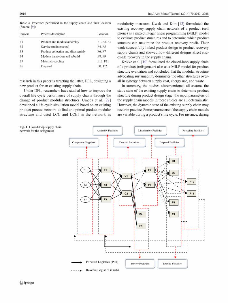
Table 2 Processes performed in the supply chain and their location(Source: [9])

Process Process description Location

P1 Product and module assembly F1, F2, F3

P2 Service (maintenance) F4, F5

P3 Product collection and disassembly F6, F7

P4 Module inspection and rebuild F8, F9

P5 Material recycling F10, F11

P6 Disposal D1, D2


January 2009 to January 2011, Brent barrel oil contract pricewas soaring from $40 to $120 (US [24]). The rise of the fuelprice obviously led to the significant increase of not only

transportation cost but also the manufacturing cost. Addition-ally, US fuel economy regulations were first introduced in1975 and demanded the production of more fuel-efficient

Fig. 5 Location of the demands and the facilities in Europe on a Google map

Table 3 Distance matrix of the supply chain network (Source: [9])

F1 F2 F3 F4 F5 F6 F7 F8 F9 F10 F11 C1 C2 D1 D2

F1 0

F2 600 0

F3 410 490 0 Symmetric

F4 220 430 200 0

F5 790 500 470 580 0

F6 1290 880 1020 1080 510 0

F7 1070 1340 860 1020 1050 1470 0

F8 720 1130 690 720 1100 1590 470 0

F9 1370 1200 970 1160 680 1290 1150 1410 0

F10 560 670 210 370 520 990 640 630 910 0

F11 1520 1680 1280 1470 1390 1540 510 990 1250 1080 0

C1 770 780 400 580 470 860 680 730 690 220 920 0

C2 480 160 350 290 380 840 1140 1030 1200 520 1560 740 0

D1 1120 950 720 910 450 430 970 1160 250 680 1140 450 970 0

D2 1340 850 1100 1130 610 290 1650 1710 680 1110 1830 1070 840 690 0


vehicles. According to the regulations, the fuel economystandard for light trucks in miles per gallon (MPG) increasedabout 15 % from 2006 to 2011 and is expected to increaseabout 14 % from 2012 to 2017 [14, 15]. This fact necessitatescompanies to pay close attention to energy savings to reduceenvironmental impacts and prevent from a potential penaltyagainst the regulations. In situations such as the one men-tioned above, the new product designed for the static supplychain may not be optimal throughout its life cycle if the supplychain effects on the product exist. This potential motivates usto investigate the supply chain effects on product modularstructures. Krikke et al. [10] have used sensitivity analysis toexplore the impact of supply chain factors (rate of return,recovery feasibility, recovery target) on product life cycleperformance. Insufficiently, only the effect of individual sup-ply chain factors was discussed and the compound effect ofmultiple factors was not considered. In addition, their workanalyzed the supply chain effect using only one single mod-ular structure and did not probe the potential of modularstructures to improve product life cycle performance. Thispaper explores the different supply chain factors from theirwork and overcome these drawbacks.

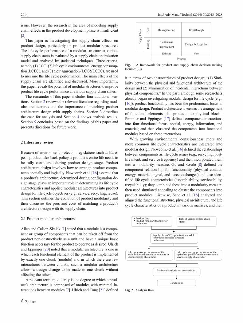
3 Analysis flow

This section presents the analysis flow to investigate thesupply chain effects on the product as shown in Fig. 2.First, we specify a modular structure of a target product

and then input the associated product data into a supplychain optimization model for product modular structureevaluation along with various supply chain states. Thissupply chain model was in our earlier work [4] and canbe used to evaluate the life cycle performance of asingle modular structure and also to optimize modularstructures. Through this supply chain model, the lifecycle performances of the evaluated modular structureand the optimized one, both at various supply chainstates are calculated. The data set of the product lifecycle performance outputted from the supply chainmodel is analyzed statistically and then compared withthe optimized modular structure. Based on the analysisresults, a conclusion is made. These steps are explainedin further details below.

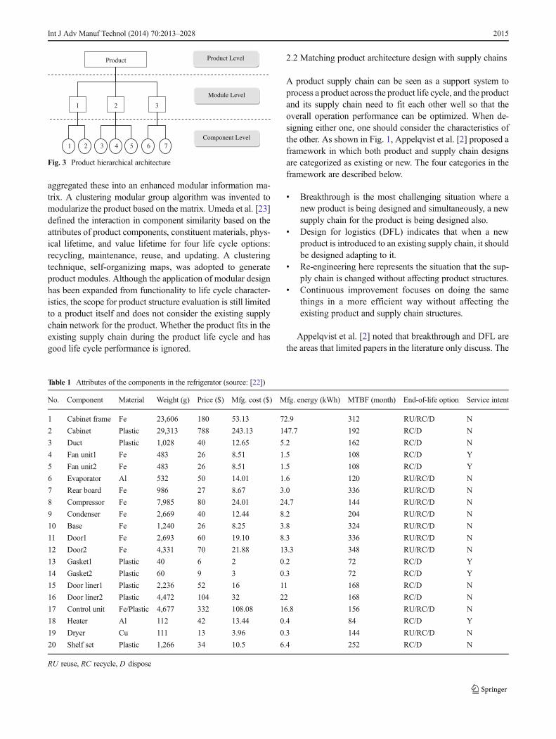
3.1 Product description

The product architecture in this paper is divided into threelevels: product, module, and component as illustrated inFig. 3. Echoing Allen and Calson-Skalak’s definition inSection 2, a module is defined as a set of components.The number of components in a module is greater than orequal to one. Any component in a module must havefunctional interactions or physical contact with other com-ponents in the module. The components are grouped intomodules, and the product modular structure consists ofthese modules. The target product in this paper is arefrigerator consisting of 20 components, and its related

Table 4 Capacity levels of dis-assembly, rebuild, and recyclingcapacity

*the level at the original supplychain state used as a baseline forcomparison

Factor (unit)/factor level High Low Difference description

A: Disassembly capacity (labor hours) 3,343.7* 2,229.2 High→ low: 50 % decrease

B: Rebuild capacity (labor hours) 3,125.0* 2,083.4* High→ low: 50 % decrease

C: Recycling capacity (tons) 331.2* 220.8 High→ low: 50 % decrease

D: Unit transp. cost (US dollars per km ton) 0.24 0.16* Low→ high: 50 % increase

E: Unit transp. energy Consumption (kWh per km ton) 0.8* 0.4 High→ low: 50 % decrease

The LCC at

7.9%

original SC state

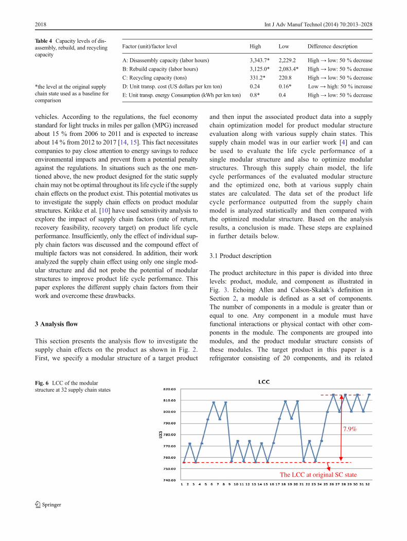
Fig. 6 LCC of the modularstructure at 32 supply chain states


data for analysis are culled from Umeda et al. [22] aslisted in Table 1.

Table 1 contains most of the information for LCC andLCEC calculation, like weight, price, manufacturing cost,etc. Manufacturing cost and energy denote the cost and energyconsumed for making a component prior to the product/module assembly process. MTBF stands for “mean time be-tween failures.” It indicates the potential component lifetimeand its reciprocal implies the service frequency of the compo-nent during the product life cycle. The end-of-life optionsinclude reuse (RU), recycling (RC), and disposal (D) andmay be used alone or in combination. These options usuallydepend on life cycle profitability. Reuse has a greater potentialamong end-of-life (EOL) options to reduce cost and to in-crease sustainability [11] so it is the first priority option inproduct modularization, recycling is the second priority optionand disposal is the last. Some components have a short life-time and need to be maintained or repaired periodically duringproduct use. Therefore, service intent denotes whether or notthe component needs to be serviced in the product life cycle;this depends on MTBF and designer’s judgment.

The modular structure for the analysis is the one with theminimal ZLCC&LCEC. ZLCC&LCEC is a bi-criteria objectivefunction aggregating LCC and LCEC and will be detailedlater in this section.

3.2 Supply chain model

Because this paper is investigating the LCC and LCEC, thesupply chain network for the refrigerator is defined as aclosed-loop supply chain network. The data set of theclosed-loop supply chain network is culled from Krikkeet al.’s [9] work. The network includes six processes per-formed at module and product assembly facilities, demandlocations, service facilities, disassembly facilities, rebuildingfacilities, recycling facilities, and disposal facilities as shownin Table 2. At the product manufacturing stage, the compo-nents are assembled into modules, and these modules areassembled into a product at the assembly facilities. At theproduct use stage, the service modules are maintained by theservice facilities. At the product retirement stage, the productis disassembled into modules, and then an EOL option foreach module is determined as reuse, recycling, or disposalbased on life cycle benefit maximization. These activities inthe supply chain are illustrated in Fig. 4.

The demand locations (C1 and C2) and the facility loca-tions (F1∼F11, D1, D2) for the product are spread acrossEurope as shown in Fig. 5, and the distances between thelocations are summarized in a distance matrix (Table 3). In2011, Chung et al. proposed a methodology using a supplychain optimization model to evaluate the life cycle

The LCEC at original SC state

6.5%

12.8%

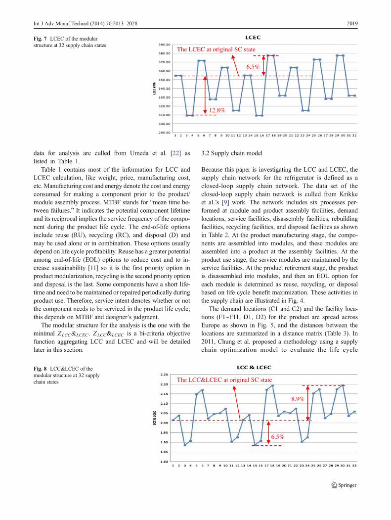
Fig. 7 LCEC of the modularstructure at 32 supply chain states

The LCC&LCEC at original SC state

8.9%

6.5%

Fig. 8 LCC&LCEC of themodular structure at 32 supplychain states


performance of product modular structure in terms of LCCand LCEC. In this work, a product is mapped into a functionalmodel represented by a component-and-interaction connectiv-ity graph. Each component has unique attributes, and theirinteractions have been defined as function, joining, anddisjoining. The estimation of a product’s LCC and LCEC isbased on both the component attributes and the interactionsbetween them. The supply chain optimizationmodel is createdto model the existing process facilities in the closed-loopsupply chain, and the model’s parameters are adapted tovarious modular structures. Additionally, an effective heuristicis developed as the methodology to determine an optimalmodular structure with the best life cycle performance. UsingChung et al.’s methodology, a designer is then able to identifynot only the most beneficial modular structure during theconfiguration design but also an optimal supply chain alloca-tion for the identified modular structure.

This paper will use this methodology to evaluate the lifecycle performance of the modular structure with the minimalZLCC&LCEC (mentioned in Section 3.1) at various supplychain states and identify the life cycle performance of theoptimized structure at each state for comparison. The mathe-matical form of this supply chain model is shown inAppendix A.

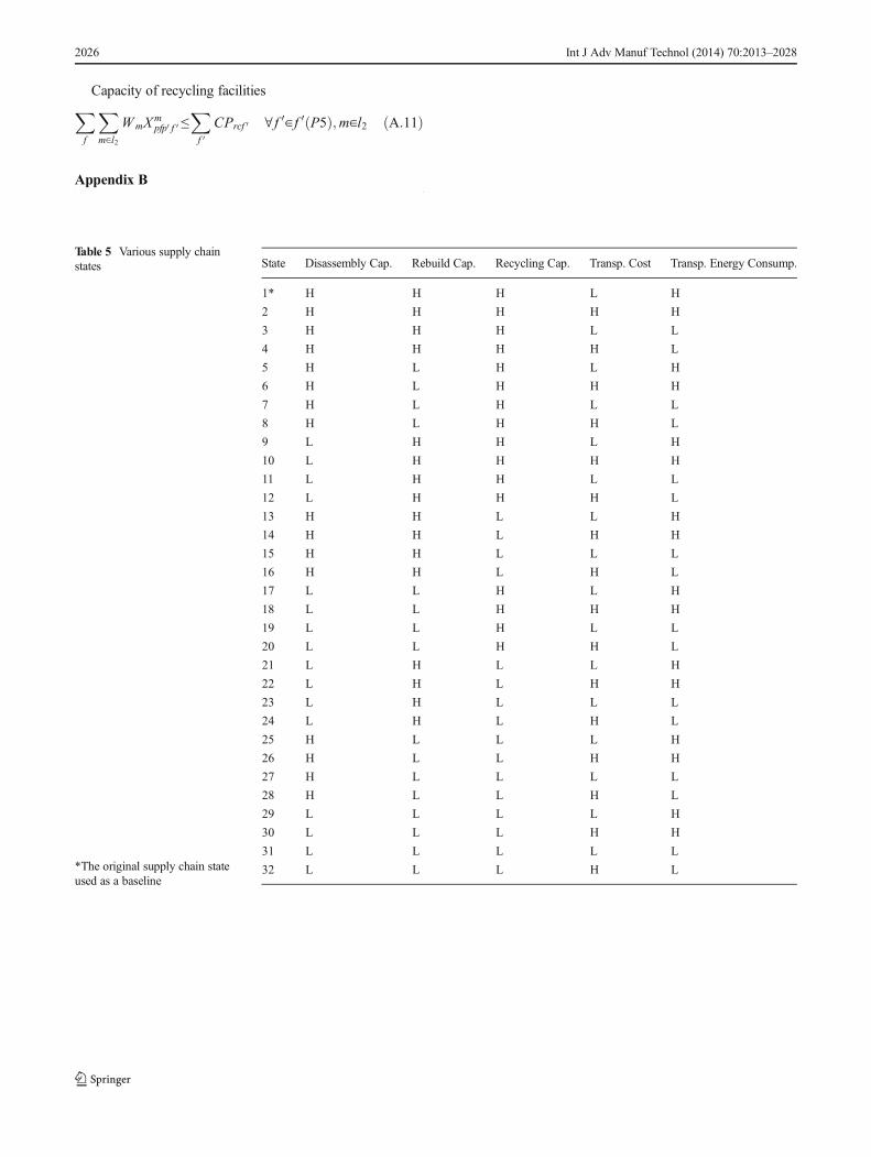
3.3 Various supply chain states

The supply chain states in this paper are determined by fiveselected factors in the supply chain: (1) disassembly capacity(factor A), (2) rebuild capacity (factor B), (3) recycling capacity(factor C), (4) unit transportation cost (factor D), and (5) unittransportation energy consumption (factor E). In general, dur-ing reverse logistics in a closed-loop supply chain, many var-ious existing products may be processed in product recoveryfacilities simultaneously (e.g., disassembly facilities, rebuildfacilities, and recycling facilities). When a new product isintroduced into the existing supply chain, it has to competewith the other existing products for the capacities of the recov-ery activities. The capacities in the recovery facilities are usu-ally limited for each type of product to be processed. Therefore,the capacities in the recovery facilities, i.e., disassembly capac-ity, rebuild capacity, and recycling capacity, are selected as thefactors to generate various supply chain states. Additionally, asaforementioned in Section 2, we are interested in the influenceof oil price fluctuation and environmental regulations; accord-ingly, unit transportation cost and energy consumption in thesupply chain are also selected as the variable factors.

These selected factors affect the parameters in the supplychain model. Each factor has two levels, high and low, and the

The LCC at the original SC state

30% Imprv. 82% Imprv.

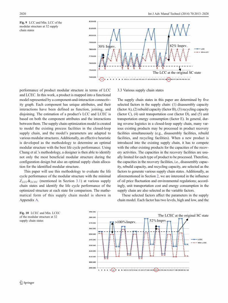
Fig. 9 LCC andMin. LCC of themodular structure at 32 supplychain states

The LCEC at the original SC state

52 Imprv.>100 Imprv.

Fig. 10 LCEC and Min. LCECof the modular structure at 32supply chain states


factor levels are summarized in Table 4. The original supplychain state is the case study used in Chung et al.’s work [4] andis used as a baseline for comparison between various supplychain states. Its factor levels are labeled with a star sign (*) inTable 4. For disassembly, rebuild, and recycling capacities andunit transportation energy consumption, the factor levels at theoriginal supply chain state are considered to be at their “high”

levels, and they decrease by 50 % to “low” are considered aswell. For unit transportation cost, the factor level at the orig-inal supply chain state is considered as “low” and thus it isincreased by 50 % to “high.”With the five factors and the twofactor levels, 32 supply chain states (23=32) are generated asshown in Appendix B. State 1 in Appendix B is the originalsupply chain state.

The LCC&LCEC at the original SC state

31 Imprv.

79 Imprv.

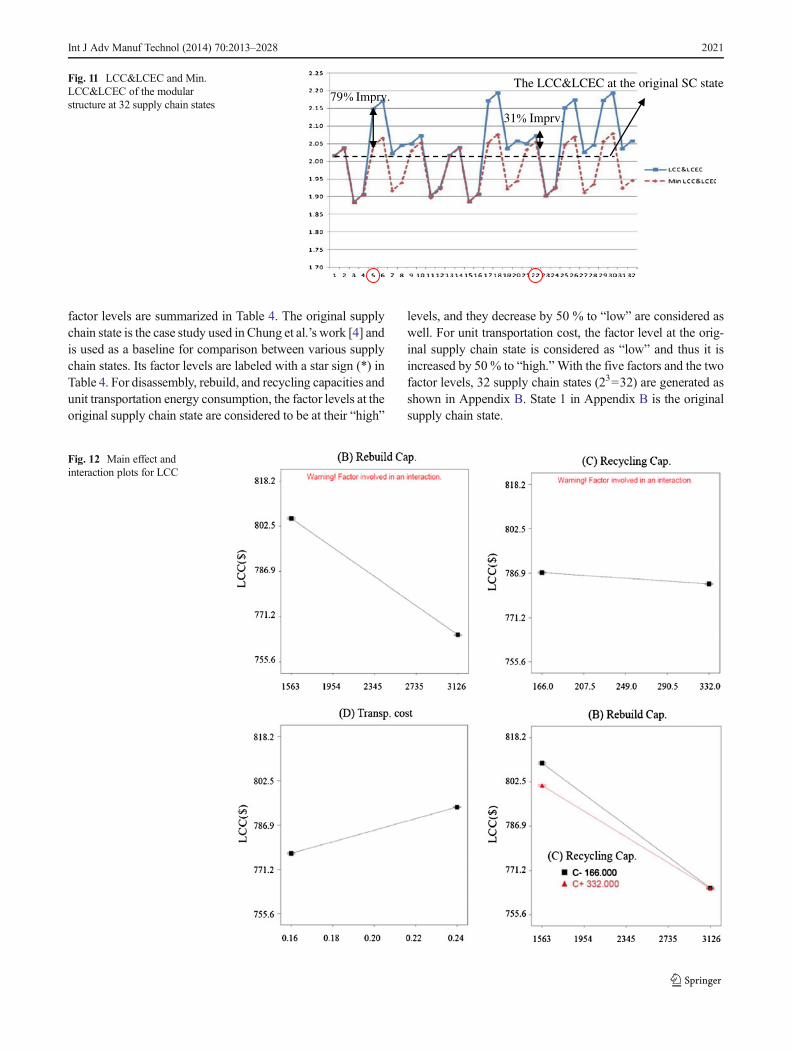
Fig. 11 LCC&LCEC and Min.LCC&LCEC of the modularstructure at 32 supply chain states

Fig. 12 Main effect andinteraction plots for LCC


3.4 Evaluation criteria for product modular structures

During product design, many factors (e.g., functionality, man-ufacturability, cost, etc.) need to be considered simultaneously;thus, multiple criteria optimization is a common technique usedin trade-off decision making in product design. The LCCrepresents the view from the side of economic feasibility, andthe LCEC represents the view from the side of environmentalimpact. To balance the two sides and facilitate trade-off decisionmaking between LCC and LCEC in modular design, besidestwo single criteria (LCC and LCEC) already used as the objec-tive in the supply chain optimization model to identify the bestmodular structure (Equation (A.1) and Equation (A.2) inAppendix A), a bi-criteria objective function aggregatingLCC and LCEC, ZLCC&LCEC, is used as the third evaluationcriterion for product modular structures and is proposed asbelow.

Minimize

ZLCC&LCEC ¼ ZLCC

MinLCCþ ZLCEC

MinLCECð1Þ

where

ZLCC is the life cycle cost in the supply chain (USdollars). It is provided in further detail in Equation(A.1) of Appendix A.

ZLCEC is the life cycle energy consumption in the supplychain (kilowatt hour). Further explanation isprovided in Equation (A.2) of Appendix A.

MinLCC

is the minimal LCC of the true optimal modularstructure for LCC at the original supply chain state.

MinLCEC

is the minimal LCEC of the true optimal modularstructure for LCEC at the original supply chain state.

Since the two single objectives, ZLCC and ZLCEC in Eq. (1),are measured in different units, US dollars and kilowatt hour,respectively, the bi-criteria objective function needs to normalizethem before their aggregation. “Min LCC” and “Min LCEC”represent the minimal LCC and LCEC of the true optimalmodular structure for LCC and LCEC at the original supplychain state, respectively. They are used to divide the two singleobjectives, ZLCC and ZLCEC, and then turn them into the ratiosso the two objectives can be aggregated into one objective.

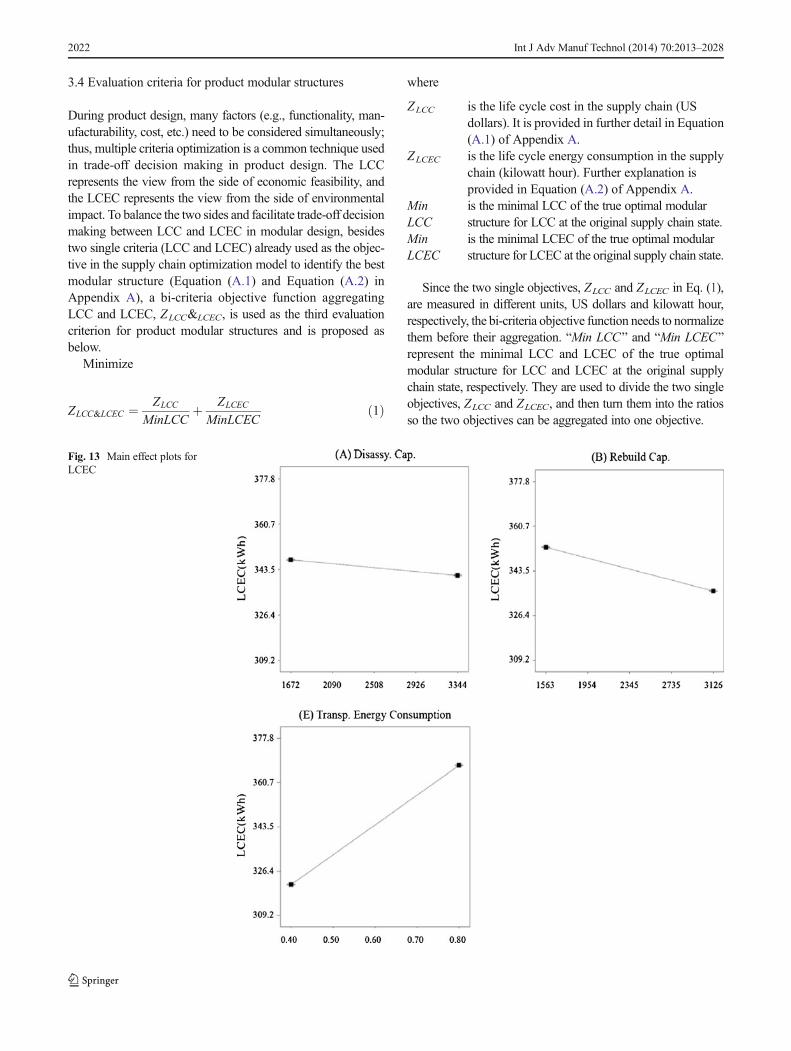
Fig. 13 Main effect plots forLCEC


4 Results

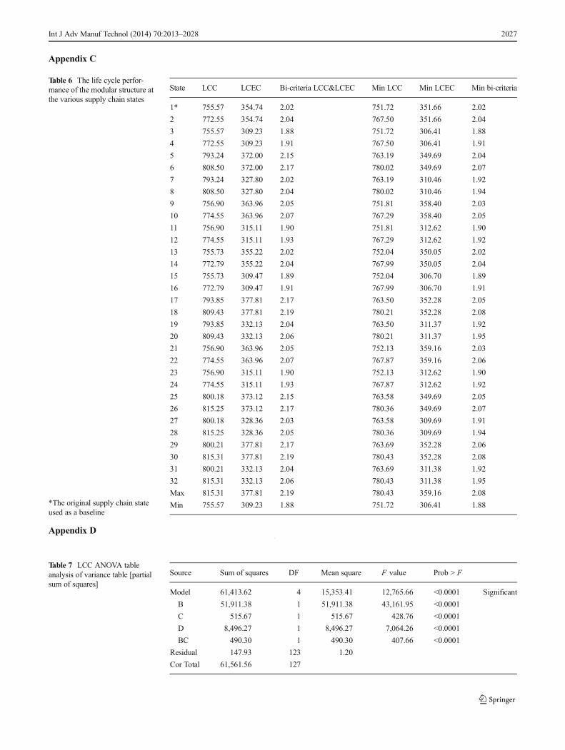
Using the analysis flow outlined and the case described inSection 3, the life cycle performances of the modular structureat the 32 supply chain states are calculated, summarized inAppendix C, and illustrated in Figs. 6, 7, and 8. As inAppendix B, state 1 in Appendix C is also the original supplychain state. Under the 32 supply chain states, the change inLCC of the modular structure in comparison to the originalstate ranges between increases of 7.9 and 0 %. The similarchange for LCEC of the modular structure ranges between6.5 % increase and 12.8 % decrease. In other words, theoverall difference between the best state and the worst stateis about 20 %. The LCC&LCEC of the modular structurechanges from the original state between 8.9 % upward and6.5 % downward. The overall difference between the beststate and the worst state is about 16 %.

The best life cycle performance (minimal LCC, minimalLCEC, and minimal LCC&LCEC) that can be reachedthrough the change of modular structures is also summarizedin Appendix C and plotted in Figs. 9, 10, and 11, respectively.

The difference between the square data points (connected bythe solid line segments) and the diamond data points (con-nected by the dotted line segments) represents the potentialimprovement that can be reached. It is observed that theimprovement at some states is significant (e.g., states 5∼8,17∼20, 25∼32). These states all involve the low-level rebuildcapacity. This implies that an optimized modular structure isparticularly effective to improve the product life cycle perfor-mance at the supply chain states with insufficient rebuildcapacity. For the states with the surge over the original SCstate, the improvement for LCC can reach at least 30 and upto 82 % (e.g., states 2 and 25 in Fig. 9); the improvement forLCEC can reach at least 52 and even exceed 100 % offset-ting the LCEC increase caused by the supply chain states(e.g., states 6 and 21 in Fig. 10); the improvement forLCC&LCEC can reach at least 31 and up to 79 % (e.g.,states 5 and 22 in Fig. 11).

Besides the life cycle performance and the potential im-provement at the various supply chain states, we also investi-gated the significance level of the factor effects on the lifecycle performance. Analysis of variance (ANOVA) is used to

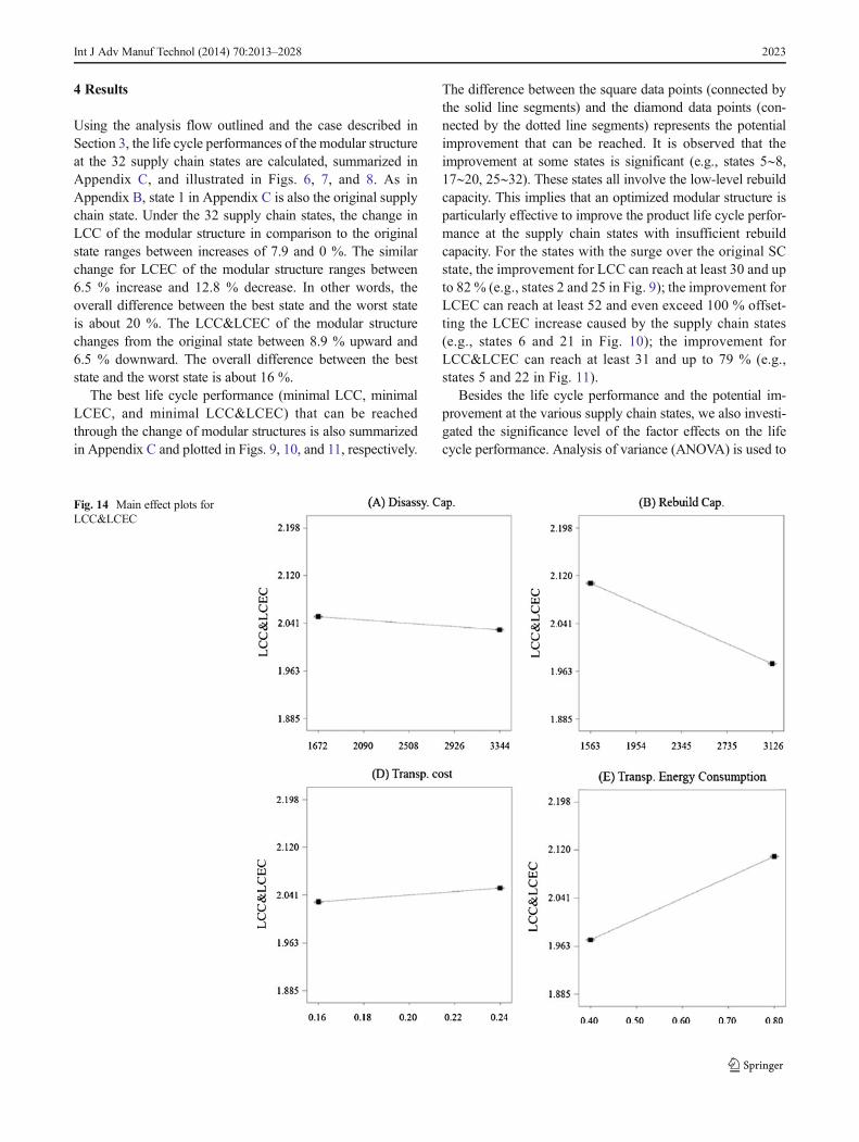
Fig. 14 Main effect plots forLCC&LCEC


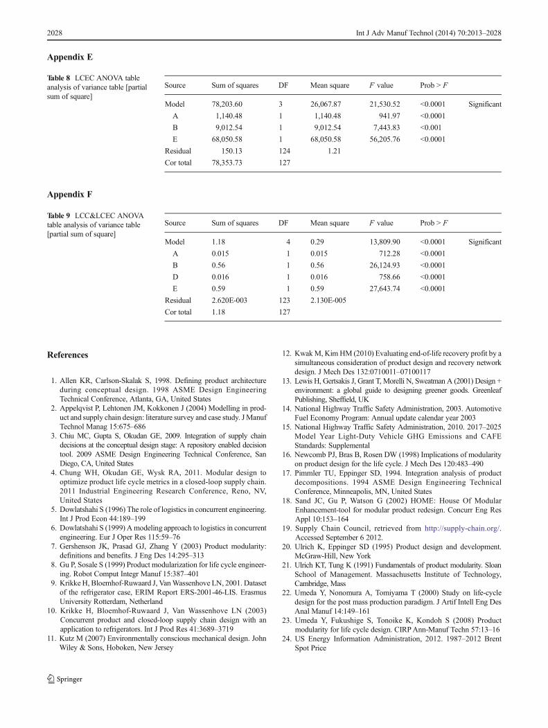
analyze the data set in Appendix C (the software used for theanalysis: Design Expert version 6.0.3). The main effect factorsare identified and the associated ANOVA tables are shown inAppendix D∼F. For LCC, rebuild capacity (B) has a negativeeffect on LCC (the upper left in Fig. 12), and unit transporta-tion cost (D) has a positive effect on LCC (the lower left inFig. 12). Recycling capacity (C) has a small effect on LCC butit has an interaction with rebuild capacity (B) as shown in thelower right in Fig. 12.

Disassembly capacity (A) affects LCEC only a little asshown in the upper left in Fig. 13. Rebuild capacity (B) hasa negative effect on LCEC (the upper right in Fig. 13), andunit transportation energy consumption (E) has a positiveeffect on LCEC (the lower left in Fig. 13).

When LCC and LCEC are aggregated as the bi-criteriaobjective LCC&LCEC, rebuild capacity (B) has a negativeeffect (the upper right in Fig. 14), and unit transportationenergy consumption (E) has a positive effect on LCC&LCEC(the lower right in Fig. 14). Yet, disassembly capacity (A) andunit transportation cost (D) both generate small effects asshown in the upper left and the lower left in Fig. 14.

5 Conclusion and future work

Based on the proposed case study and the results above, themain findings are that the various supply chain states do signif-icantly affect the life cycle performance of the modular structurein the supply chain. The fluctuation of the life cycle perfor-mance (the gap between the best state and the worst state) issignificant (8 % in LCC, 20 % in LCEC, and 16 % inLCC&LCEC). The results also reveal that modular structureoptimization is effective to reduce LCC and LCEC surge causedby the various supply chain states. For LCC, the reductionranges from 30 to 82 %. For LCC&LCEC, the reduction rangesfrom 31 to 79 %. For LCEC, the reduction can even completelyoffset the surge. In addition, the main supply chain effects onproduct life cycle performance are identified. This finding pavesthe way for the development of methods in product designtaking into account the supply chain implications.

Although insightful, we consider our work here to bepreliminary; more research efforts are required to garner gen-eral observations. For instance, only five factors are selectedto generate the various supply chain states. These factors maynot be sufficient to model a complicated and dynamic supplychain network. Moreover, product modular structures are theonly variable considered to improve the product life cycleperformance in the supply chain. Other variables in productdesign, such as material selection, manufacturing processselection, etc., can be integrated in the proposed model forfurther improvement in the life cycle performance. Most

importantly, an effective method needs to be developed toidentify robust product architecture to fit into the dynamicsof the supply chains.

Acknowledgments This work was funded under a collaborative Ad-vanced CyberInfrastructure (ACI) program at the National Science Foun-dation (Grant No. ACI-1041328). Any opinions, findings, and conclu-sions or recommendations presented in this paper are those of the authorsand do not necessarily reflect the views of the National ScienceFoundation.

Appendix A: mathematical model of the supply chain

Index sets

A = {a1, a2,…, a20} Set of componentsM = {m1, m2, …} Set of modules (the number of

modules depends on various modularstructures; the maximum is less thanthe number of components)

S = {s1, s2, s3} Set of component suppliersC = {c1, c2} Set of demand locationsF = {f1, f2, …, f11} Set of facilities for processesD = {d1, d2} Set facilities for disposalP = {p1, p2, …, p6} Set of processes in the supply chainL = {l1, l2, l3} Set of service and EOL options:

l1 = reuse, l2 = recycling, l3 = disposal,l4 = service

Decision variables

Xspfa Component flow from component supplier s to facility

f for process pXpfc Product flow from process p in facility f to demand

location cXcpf Product flow from demand location c to process p in

facility fXpfc

a Component flow between facility f and demandlocation c for process p

Xpfcm Module flow between facility f and demand location c

for process pXpfp ′f ′

m Module flow from process p in facility f to process p ′in facility f ′

Xpfdm Module flow from facility f to facility d for disposal

Parameters

a The return rate of product after useCtff ′ The unit transportation cost between facility f and

facility f ′Etff ′ The unit transportation energy consumption

between facility f and facility f ′Gc The product demand at demand location c


CPruf The rebuild capacity at facility fCPrcf The recycling capacity at facility fCPdf The disassembly capacity at facility fWm The weight of module mW The weight of productCSm The service cost of module mRrem.m The reuse return of module mRrecy.m The recycling return of module mCdisp.m The disposal cost of module mESm The service energy consumption of module mSrem.m The reuse energy saving of module mSrecy.m The recycling energy saving of module m

Edisp.m The disposal energy consumption of module mTdm The disassembly time of module mTrm The rebuild time of module m

Objective function

Min ZLCC

Min ZLCEC

where

ZLCC The life cycle cost in the supply chain (US dollars)ZLCEC The life cycle energy consumption in the supply

chain (kilowatt hour)

ZLCC ¼ CM

X

f ∈p1

X

c

X pfc þX

f ∈p2

X

f 0∈p1

X

m∈l4

CSmXmpfp0 f 0−

X

f ∈p3

X

f 0∈p4

X

m∈l1

Rrem:mXmpfp0 f 0−

X

f ∈p3

X

f 0∈p4

X

m∈l2

Rrecy:mXmpfp0 f 0 þ

X

f ∈p3

X

d

X

m∈l3

Cdisp:mXmpfd

þX

f

X

c

WCtfcX pfc þX

c

X

f

WCtcf 0X cpf þX

f ∈p2

X

f 0∈p1

X

m∈l4

WmCtff 0Xmpfp0 f 0 þ

X

f ∈p3

X

f 0∈p4

X

m∈l1

WmCtff 0Xmpfp0 f 0 þ

X

f ∈p3

X

f 0∈p4

X

m∈l2

WmCtff 0Xmpfp0 f 0

þX

f ∈p3

X

d

X

m∈l3

WmCtff 0Xmpfd

ðA:1Þ

ZLCEC ¼ EM

X

f ∈p1

X

c

X pfc þX

f ∈p2

X

f 0∈p1

X

m∈l4

ESmXmpfp0 f 0−

X

f ∈p3

X

f 0∈p4

X

m∈l1

Srem:Xmpfp0 f 0−

X

f ∈p3

X

f 0∈p4

X

m∈l2

Srecy:mXmpfp0 f 0 þ

X

f ∈p3

X

d

X

m∈l3

Edisp:mXmpfd

þX

f

X

c

EtfcX pfc þX

c

X

f

Etcf 0X cpf þX

f ∈p2

X

f 0∈p1

X

m∈l4

Etff 0Xmpfp0 f 0 þ

X

f ∈p3

X

f 0∈p4

X

m∈l1

Etff 0Xmpfp0 f 0 þ

X

f ∈p3

X

f 0∈p4

X

m∈l2

Etff 0Xmpfp0 f 0 þ

X

f ∈p3

X

d

X

m∈l3

Etff 0Xmpfd

ðA:2ÞFlow balance constraints

Flow balance at product/module assembly facilities (P1:F1∼F3)X

s

X aspf ¼

X

c

X pfc ∀a∀ f ∈ f P1ð Þ ðA:3Þ

Flow balance at demand locationsX

f

X pfc ¼ Gc ∀c ðA:4Þ

X

f

X cpf ¼ αGc ∀c ðA:5Þ

Flow balance at service facilities (P2: F4∼F5)X

f

X mpfp0 f 0 ¼

X

c

X mpfc ∀m∈l4∀ f 0∈ f P2ð Þ ðA:6Þ

Flow balance at collection and disassembly facilities (P3:F6∼F7)

X

c

X cpf ¼X

f 0Xm

pfp0 f 0 þX

d

X mpfd ∀m∀ f ∈ f P3ð Þ; f 0∈ f P4;P5ð ÞðA:7Þ

Flow balance at rebuild facilities (P4: F8∼F9)X

f

X mpfp0 f 0 ¼

X

f 0 0Xm

p0 f 0p0 0 f 0 0 ∀m∈l1∀ f 0∈ f 0 P4ð Þ; f 00∈ f P1ð Þ

ðA:8Þ

Capacity constraints

Capacity of disassembly facilities

X

f 0

X

m

TdmXmpfp0 f 0 þ

X

d

X

m

TdmXmpfd ≤CPdf ∀ f ∈ f P3ð Þ; f 0∈ f P4;P5ð Þ

ðA:9Þ

Capacity of rebuild facilities

X

f

X

m∈l1

TrmXmpfp0 f 0 ≤

X

f 0CPruf 0 ∀ f 0∈ f 0 P4ð Þ;m∈l1 ðA:10Þ


Capacity of recycling facilitiesX

f

X

m∈l2

WmXmpfp0 f 0 ≤

X

f 0CPrcf 0 ∀ f 0∈ f 0 P5ð Þ;m∈l2 ðA:11Þ

Appendix B

Table 5 Various supply chainstates

*The original supply chain stateused as a baseline

State Disassembly Cap. Rebuild Cap. Recycling Cap. Transp. Cost Transp. Energy Consump.

1* H H H L H

2 H H H H H

3 H H H L L

4 H H H H L

5 H L H L H

6 H L H H H

7 H L H L L

8 H L H H L

9 L H H L H

10 L H H H H

11 L H H L L

12 L H H H L

13 H H L L H

14 H H L H H

15 H H L L L

16 H H L H L

17 L L H L H

18 L L H H H

19 L L H L L

20 L L H H L

21 L H L L H

22 L H L H H

23 L H L L L

24 L H L H L

25 H L L L H

26 H L L H H

27 H L L L L

28 H L L H L

29 L L L L H

30 L L L H H

31 L L L L L

32 L L L H L


Appendix C

Appendix D

Table 6 The life cycle perfor-mance of the modular structure atthe various supply chain states

*The original supply chain stateused as a baseline

State LCC LCEC Bi-criteria LCC&LCEC Min LCC Min LCEC Min bi-criteria

1* 755.57 354.74 2.02 751.72 351.66 2.02

2 772.55 354.74 2.04 767.50 351.66 2.04

3 755.57 309.23 1.88 751.72 306.41 1.88

4 772.55 309.23 1.91 767.50 306.41 1.91

5 793.24 372.00 2.15 763.19 349.69 2.04

6 808.50 372.00 2.17 780.02 349.69 2.07

7 793.24 327.80 2.02 763.19 310.46 1.92

8 808.50 327.80 2.04 780.02 310.46 1.94

9 756.90 363.96 2.05 751.81 358.40 2.03

10 774.55 363.96 2.07 767.29 358.40 2.05

11 756.90 315.11 1.90 751.81 312.62 1.90

12 774.55 315.11 1.93 767.29 312.62 1.92

13 755.73 355.22 2.02 752.04 350.05 2.02

14 772.79 355.22 2.04 767.99 350.05 2.04

15 755.73 309.47 1.89 752.04 306.70 1.89

16 772.79 309.47 1.91 767.99 306.70 1.91

17 793.85 377.81 2.17 763.50 352.28 2.05

18 809.43 377.81 2.19 780.21 352.28 2.08

19 793.85 332.13 2.04 763.50 311.37 1.92

20 809.43 332.13 2.06 780.21 311.37 1.95

21 756.90 363.96 2.05 752.13 359.16 2.03

22 774.55 363.96 2.07 767.87 359.16 2.06

23 756.90 315.11 1.90 752.13 312.62 1.90

24 774.55 315.11 1.93 767.87 312.62 1.92

25 800.18 373.12 2.15 763.58 349.69 2.05

26 815.25 373.12 2.17 780.36 349.69 2.07

27 800.18 328.36 2.03 763.58 309.69 1.91

28 815.25 328.36 2.05 780.36 309.69 1.94

29 800.21 377.81 2.17 763.69 352.28 2.06

30 815.31 377.81 2.19 780.43 352.28 2.08

31 800.21 332.13 2.04 763.69 311.38 1.92

32 815.31 332.13 2.06 780.43 311.38 1.95

Max 815.31 377.81 2.19 780.43 359.16 2.08

Min 755.57 309.23 1.88 751.72 306.41 1.88

Table 7 LCC ANOVA tableanalysis of variance table [partialsum of squares]

Source Sum of squares DF Mean square F value Prob > F

Model 61,413.62 4 15,353.41 12,765.66 <0.0001 Significant

B 51,911.38 1 51,911.38 43,161.95 <0.0001

C 515.67 1 515.67 428.76 <0.0001

D 8,496.27 1 8,496.27 7,064.26 <0.0001

BC 490.30 1 490.30 407.66 <0.0001

Residual 147.93 123 1.20

Cor Total 61,561.56 127


Appendix E

Appendix F

References

1. Allen KR, Carlson-Skalak S, 1998. Defining product architectureduring conceptual design. 1998 ASME Design EngineeringTechnical Conference, Atlanta, GA, United States

2. Appelqvist P, Lehtonen JM, Kokkonen J (2004) Modelling in prod-uct and supply chain design: literature survey and case study. JManufTechnol Manag 15:675–686

3. Chiu MC, Gupta S, Okudan GE, 2009. Integration of supply chaindecisions at the conceptual design stage: A repository enabled decisiontool. 2009 ASME Design Engineering Technical Conference, SanDiego, CA, United States

4. Chung WH, Okudan GE, Wysk RA, 2011. Modular design tooptimize product life cycle metrics in a closed-loop supply chain.2011 Industrial Engineering Research Conference, Reno, NV,United States

5. Dowlatshahi S (1996) The role of logistics in concurrent engineering.Int J Prod Econ 44:189–199

6. Dowlatshahi S (1999) Amodeling approach to logistics in concurrentengineering. Eur J Oper Res 115:59–76

7. Gershenson JK, Prasad GJ, Zhang Y (2003) Product modularity:definitions and benefits. J Eng Des 14:295–313

8. Gu P, Sosale S (1999) Product modularization for life cycle engineer-ing. Robot Comput Integr Manuf 15:387–401

9. KrikkeH, Bloemhof-Ruwaard J, VanWassenhove LN, 2001. Datasetof the refrigerator case, ERIM Report ERS-2001-46-LIS. ErasmusUniversity Rotterdam, Netherland

10. Krikke H, Bloemhof-Ruwaard J, Van Wassenhove LN (2003)Concurrent product and closed-loop supply chain design with anapplication to refrigerators. Int J Prod Res 41:3689–3719

11. Kutz M (2007) Environmentally conscious mechanical design. JohnWiley & Sons, Hoboken, New Jersey

12. KwakM, KimHM (2010) Evaluating end-of-life recovery profit by asimultaneous consideration of product design and recovery networkdesign. J Mech Des 132:0710011–07100117

13. Lewis H, Gertsakis J, Grant T, Morelli N, Sweatman A (2001) Design +environment: a global guide to designing greener goods. GreenleafPublishing, Sheffield, UK

14. National Highway Traffic Safety Administration, 2003. AutomotiveFuel Economy Program: Annual update calendar year 2003

15. National Highway Traffic Safety Administration, 2010. 2017–2025Model Year Light-Duty Vehicle GHG Emissions and CAFEStandards: Supplemental

16. Newcomb PJ, Bras B, Rosen DW (1998) Implications of modularityon product design for the life cycle. J Mech Des 120:483–490

17. Pimmler TU, Eppinger SD, 1994. Integration analysis of productdecompositions. 1994 ASME Design Engineering TechnicalConference, Minneapolis, MN, United States

18. Sand JC, Gu P, Watson G (2002) HOME: House Of ModularEnhancement-tool for modular product redesign. Concurr Eng ResAppl 10:153–164

19. Supply Chain Council, retrieved from http://supply-chain.org/.Accessed September 6 2012.

20. Ulrich K, Eppinger SD (1995) Product design and development.McGraw-Hill, New York

21. Ulrich KT, Tung K (1991) Fundamentals of product modularity. SloanSchool of Management. Massachusetts Institute of Technology,Cambridge, Mass

22. Umeda Y, Nonomura A, Tomiyama T (2000) Study on life-cycledesign for the post mass production paradigm. J Artif Intell Eng DesAnal Manuf 14:149–161

23. Umeda Y, Fukushige S, Tonoike K, Kondoh S (2008) Productmodularity for life cycle design. CIRPAnn-Manuf Techn 57:13–16

24. US Energy Information Administration, 2012. 1987–2012 BrentSpot Price

Table 8 LCEC ANOVA tableanalysis of variance table [partialsum of square]


Model 78,203.60 3 26,067.87 21,530.52 <0.0001 Significant

A 1,140.48 1 1,140.48 941.97 <0.0001

B 9,012.54 1 9,012.54 7,443.83 <0.001

E 68,050.58 1 68,050.58 56,205.76 <0.0001

Residual 150.13 124 1.21

Cor total 78,353.73 127

Table 9 LCC&LCEC ANOVAtable analysis of variance table[partial sum of square]


Model 1.18 4 0.29 13,809.90 <0.0001 Significant

A 0.015 1 0.015 712.28 <0.0001

B 0.56 1 0.56 26,124.93 <0.0001

D 0.016 1 0.016 758.66 <0.0001

E 0.59 1 0.59 27,643.74 <0.0001

Residual 2.620E-003 123 2.130E-005

Cor total 1.18 127


http://supply-chain.org/

Documents

Life cycle implications of product modular architectures in closed-loop supply chains