Embed Size (px)
Citation preview
Coordination
in
Closed-Loop Supply Chains
Inauguraldissertation zur Erlangung des akademischen
Grades eines Doktors der Wirtschaftswissenschaften der
Universitat Mannheim
vorgelegt von
Dipl.-Kffr. Carolin Zuber
Heidelberg

Dekan: Dr. Jurgen M. Schneider
Referent: Prof. Dr. Moritz Fleischmann
Korreferent: Univ.-Prof. Dr. Marc Reimann
Tag der mundlichen Prufung: 13. Marz 2015

Contents
1 An Introduction to Closed-Loop Supply Chains 1
1.1 Introduction . . . . . . . . . . . . . . . . . . . . . . . . . . . . . . . . 1
1.2 Closed-Loop Supply Chain Processes and Actors . . . . . . . . . . . . 3
1.3 Reverse Logistics at SC Service Group: An Illustrative Case . . . . . 5
1.3.1 SC Service Group . . . . . . . . . . . . . . . . . . . . . . . . . 5
1.3.2 The Asset Recovery Center and its Reverse Supply Chain . . . 6
1.4 Identified Research Needs . . . . . . . . . . . . . . . . . . . . . . . . 10
1.5 Outline of the Thesis . . . . . . . . . . . . . . . . . . . . . . . . . . . 12
2 Coordination of Multiple Decision Makers - Structuring the Field 14
2.1 Coordination in the Forward Supply Chain Literature . . . . . . . . . 14
2.1.1 How to Coordinate Actions in Decentralized Supply Chains . . 15
2.1.2 How to Coordinate Actions and Pursue Information Transfer
in Decentralized Supply Chains . . . . . . . . . . . . . . . . . 18
2.2 Coordination in the Closed-Loop Supply Chain Literature . . . . . . 21
3 Coordination in Closed-Loop Supply Chains - The Case of the Dis-
position Decision 27
3.1 Literature Review - Disposition Decisions in Closed-Loop Supply Chains 28
3.1.1 Characterizing the Disposition Decision . . . . . . . . . . . . . 28
3.1.2 Models of the Disposition Decision . . . . . . . . . . . . . . . 32
3.2 Model Assumptions and Notation . . . . . . . . . . . . . . . . . . . . 35
3.3 The Disposition Decision . . . . . . . . . . . . . . . . . . . . . . . . . 42
3.3.1 Central Decision Maker - Benchmark . . . . . . . . . . . . . . 42
3.3.2 Decentralized Decision Makers - The Situation of the Business
Case . . . . . . . . . . . . . . . . . . . . . . . . . . . . . . . . 46
3.3.3 Decentralized Decision Makers - The Service Provider Ac-
quires Product Returns . . . . . . . . . . . . . . . . . . . . . . 60
3.4 Numerical Example . . . . . . . . . . . . . . . . . . . . . . . . . . . 65
I

CONTENTS II
3.5 Discussion . . . . . . . . . . . . . . . . . . . . . . . . . . . . . . . . . 71
4 Coordination in Closed-Loop Supply Chains - The Customer In-
terface 76
4.1 Introduction . . . . . . . . . . . . . . . . . . . . . . . . . . . . . . . . 76
4.2 Decisions of Customers and How They Affect Closed-Loop Supply
Chain Processes . . . . . . . . . . . . . . . . . . . . . . . . . . . . . . 80
4.2.1 Customer Acquires the Product . . . . . . . . . . . . . . . . . 83
4.2.2 Customer’s Disposition Decision . . . . . . . . . . . . . . . . . 84
4.2.3 Duration of Usage . . . . . . . . . . . . . . . . . . . . . . . . 86
4.2.4 Intensity of Usage . . . . . . . . . . . . . . . . . . . . . . . . . 87
4.2.5 Demand for (Maintenance) Services . . . . . . . . . . . . . . . 89
4.2.6 Demand for Complementary Products . . . . . . . . . . . . . 90
4.3 Identified Coordination Needs at the Customer Interface . . . . . . . 93
4.4 Mechanisms to Coordinate the Coordination Issues at the Customer
Interface . . . . . . . . . . . . . . . . . . . . . . . . . . . . . . . . . . 97
4.4.1 Incentivize the Closed-Loop Supply Chain Optimal Acquisi-
tion Quantities . . . . . . . . . . . . . . . . . . . . . . . . . . 97
4.4.2 Initiating Closed-Loop Supply Chain Optimal Reverse Flows . 98
4.5 Discussion . . . . . . . . . . . . . . . . . . . . . . . . . . . . . . . . . 106
5 Conclusion 108
Bibliography 112
About the Author 121

List of Figures
1.1 Common Closed-Loop Supply Chain Processes . . . . . . . . . . . . . 4
1.2 Physical Flows of Leased IT Equipment and Actors Involved . . . . . 7
1.3 Process Steps at the Asset Recovery Center . . . . . . . . . . . . . . 8
3.1 Categorization of Disposition Options . . . . . . . . . . . . . . . . . . 30
3.2 Considered Reverse Supply Chain . . . . . . . . . . . . . . . . . . . . 36
3.3 Sequence of Events and Decisions . . . . . . . . . . . . . . . . . . . . 37
3.4 Material and Financial Flow of the Integrated Channel . . . . . . . . 42
3.5 Illustration of Clip Levels . . . . . . . . . . . . . . . . . . . . . . . . 45
3.6 Material and Financial Flow of the Business Case . . . . . . . . . . . 46
3.7 Change of Profit Margins and Clip Levels Compared to the Integrated
Setting . . . . . . . . . . . . . . . . . . . . . . . . . . . . . . . . . . . 55
3.8 Resulting Profit of L . . . . . . . . . . . . . . . . . . . . . . . . . . . 55
3.9 Financial Flow Coordinated Actors . . . . . . . . . . . . . . . . . . . 61
3.10 Comparison of Clip Levels in the Benchmark and in Case of Acquisi-
tion of Returned Products . . . . . . . . . . . . . . . . . . . . . . . . 62
3.11 Profit Margins and Disposition Decision of a Central Decision Maker 68
3.12 Profit Margins for SP and Disposition Decision of a Decentral Deci-
sion Maker . . . . . . . . . . . . . . . . . . . . . . . . . . . . . . . . . 70
3.13 Split of (Additional) Reverse Supply Chain Profit Depending on the
Acquisition Price . . . . . . . . . . . . . . . . . . . . . . . . . . . . . 71
3.14 Relaxation of Assumptions and Suggested Extensions . . . . . . . . . 72
4.1 Considered Closed-Loop Supply Chain . . . . . . . . . . . . . . . . . 80
4.2 Stages of The Customer Acquisition Decision . . . . . . . . . . . . . . 81
4.3 Effects of the Customers Product Acquisition Decision . . . . . . . . 84
4.4 Effects of the Customer’s Disposition Decision . . . . . . . . . . . . . 85
4.5 Effects of the Customer’s Decision on the Duration of the Usage Phase 86
4.6 Effects of the Customer’s Decision on the Intensity of Usage . . . . . 88
III

LIST OF FIGURES IV
4.7 Effects of the Customer’s Decision to Demand (Maintenance) Services 90
4.8 Effects of the Customer’s Decision to Demand Complementary Products 91
4.9 Clustered Summary of Customer Decisions . . . . . . . . . . . . . . . 94
4.10 Customer Decisions - Summary of Effects on Closed-Loop Supply
Chain Processes and How Customers Benefit . . . . . . . . . . . . . . 101

List of Tables
3.1 Return Type-Reprocessing Pairs . . . . . . . . . . . . . . . . . . . . . 32
3.2 Example Assumption 4C . . . . . . . . . . . . . . . . . . . . . . . . . 39
3.3 Notation . . . . . . . . . . . . . . . . . . . . . . . . . . . . . . . . . . 41
3.4 Karush-Kuhn-Tucker Condition for Local Maximum . . . . . . . . . . 50
3.5 Prices on Raw Materials Market and Secondary Market . . . . . . . . 66
3.6 Reprocessing Cost Ratios . . . . . . . . . . . . . . . . . . . . . . . . . 67
3.7 Disposition Decision of a Central Decision Maker . . . . . . . . . . . 68
3.8 L’s Optimal Decision on Service Payments [in e] . . . . . . . . . . . . 69
3.9 Disposition Decision of a Decentral Decision Maker . . . . . . . . . . 69
3.10 Profits Business Case . . . . . . . . . . . . . . . . . . . . . . . . . . . 70
4.1 Summary of Effects of Customer Decisions . . . . . . . . . . . . . . . 92
4.2 Identified Coordination Needs at the Customer Interface . . . . . . . 96
4.3 Coverage of the Customer Interface by Previous Literature . . . . . . 102
V
Chapter 1
An Introduction to Closed-Loop
Supply Chains
1.1 Introduction
Against the background of scarce resources and increasing consumption worldwide,
the awareness and realization of product reuse are essential. This is reflected not
only by the increased environmental awareness of customers but also by the legisla-
tive pressure to develop environmentally friendly products and processes. However,
taking back products can also be seen as a chance for companies to gain additional
economic benefits instead of only a burden. Due to the reuse of materials or compo-
nents obtained from returned products, money can be saved. Furthermore, giving
used products a second life offers companies the chance to earn additional profits
by entering new markets. Accordingly, the consideration of reverse product flows
can be separated into the waste-stream and the market-driven perspectives (Guide
and Van Wassenhove, 2001, 2009). From a waste-stream perspective, companies
passively accept the return of products and try to conduct reprocessing activities
at the minimum costs. From a market-driven perspective, in contrast, companies
strive to maximize their profits by remarketing reprocessed returns. This research
project draws on and contributes to the value-added perspective.
The chosen focus on the value-added stream is driven by the fact that nowadays
more and more products with remaining value are being returned. The manage-
ment of these return flows represents an opportunity to obtain additional benefits
that should not be disregarded. For example, hardly used consumer returns in the
electronics sector increased by 21% from 2007 to 2011 (Bower and Maxham, 2012).
This development is attributed to the increasing importance of e-commerce, a trend
1

An Introduction to CLSCs 2
that is expected to grow further. In Germany alone, e-commerce sales of physical
goods increased from e 18.3 billion in 2010 to e 39.1 billion in 2013 (Bundesverband
E-Commerce und Versandhandel Deutschland, 2013). Another type of returns is so-
called end-of-use returns: products that have lost their value for a certain customer
segment but are still functional and may be of use to another customer segment.
This phenomenon is especially observed in fast-moving industries with short prod-
uct life cycles, such as the IT sector. These return types are of course not new, but
due to the given market developments, they require special attention nowadays. As
both kinds of product returns are still of value, these return flows should not be
seen only as a cost factor. On the contrary, the returned units should be seen as an
opportunity to generate additional profits.
In the literature, the consideration of reverse flows started in the late 1990s. The
first focus was on operational issues, such as the disassembly of returned products.
The research centered on one actor optimizing one reverse flow activity. Since then,
research in this field has evolved towards a more process-oriented perspective. This
means that no longer is only one activity considered exclusively, but the interaction
of several activities along the reverse supply chain (SC) is considered. Consequently,
no longer does only one actor need to be taken into account, but potentially multiple,
independent actors. In the last years, the scope has been further extended to a
holistic perspective. Not only reverse but forward and reverse SC processes are
considered jointly. Due to this, the traditional forward SC is extended by the reverse
flow of products and information as well as by financial flows. Therefore, in addition
to the members of a traditional SC, actors are required that are responsible for
reverse-flow-specific processes like collection, grading and disposition, reprocessing,
and reselling. These processes can be conducted by traditional SC members, as well
as by new parties.
One of the major challenges in Supply Chain Management (SCM) is to match
supply with demand. According to Tsay et al. (1999), SC-wide optimality is achiev-
able if all the decisions are made by a single decision maker who has access to all
the available information. Usually the outcome of such centralized decision mak-
ing is used as a benchmark that can be achieved by the coordination of SCs. To
achieve coordination, explicit decisions need to be made by the actors involved. Un-
fortunately, these decisions often do not comply with the actors’ own objectives.
Additionally, actors require certain information to be able to make the necessary
decisions. Unlike the case of a centralized decision maker, not all the actors in a
common SC have access to all the available information. Both unaligned incentives
of the involved actors and information asymmetry are known to be major obstacles

An Introduction to CLSCs 3
to SC coordination (e.g. Cachon, 2003; Chen, 2003).
The challenge to match supply with demand needs to be faced in a Closed-Loop
Supply Chain (CLSC) as well. Similar to the situation in a traditional forward SC,
it can be expected that information and know-how are scattered between various
members of a CLSC. Furthermore, actors have their own incentives, and decision
making is usually decentralized. In comparison with traditional SCM, further com-
plicating factors need to be considered. First is the heterogeneity of the returned
products and the resulting increased uncertainty with respect to the supply side.
The heterogeneity and uncertainty of the supplies originate from the usage phase
of the customer, during which only little or no information is transmitted to other
CLSC actors. Second, according to Guide and Van Wassenhove (2009), the com-
plexity with regard to “designing, managing and controlling CLSCs” (p.12) increases
due to the number of actors involved.
Consequently, the consideration of decentralized CLSCs raises several, consecu-
tive questions that we want to address in this thesis:
1. What are the potential coordination needs in a CLSC environment?
2. What are the appropriate coordination mechanisms?
The following section provides an introduction to CLSC actors and the processes
relevant to this thesis. Subsequently, an illustrative case is introduced (Section 1.3).
Based on the learnings taken from the business case, we state the more explicit
research questions for this thesis in Section 1.4. We close this chapter with an
outline of the thesis (Section 1.5).
1.2 Closed-Loop Supply Chain Processes and Ac-
tors
In a CLSC setting, the traditional forward SC is extended by the reverse flow of
products and information as well as by financial flows. The main processes of such
a CLSC are depicted in Figure 1.1.
We consider a forward SC consisting of three major processes: a product needs
to be developed and designed, produced, and finally delivered to the customers via
various distribution channels. The end point of the forward SC is the customers’
acquisition and use of the product.
The reverse flow of products starts with the customers’ decision to return their
products. These products are acquired by the reverse SC and need to be collected.

An Introduction to CLSCs 4
Figure 1.1: Common Closed-Loop Supply Chain Processes
Collection can be designed in multiple ways: directly from the customer, from collec-
tion points such as retailers, or via mail services (Aras et al., 2010). During the usage
phase, customers handle their products in various ways. This is why the condition
of returned products - and thus the quality of reverse SC supplies - is particularly
heterogeneous. This makes the testing and grading of returned products necessary
to obtain quality information. Depending on the reverse logistics network design,
these processes are conducted either before or after the products are transported
to the reprocessing facility. While the advantage of the first, decentralized option
is that transportation costs for worthless products can be saved, it is accompanied
by the implementation costs of decentralized grading resources (Fleischmann et al.,
2000). Based on the grading outcome, what to do with a product of a given quality
has to be determined - that is, the disposition decision has to be made. A common
categorization of the available reprocessing options was introduced by Thierry et al.
(1995). They distinguish three groups of disposition options: direct reuse, product
recovery, and waste. Depending on the chosen disposition option, reprocessed prod-
ucts are reintroduced into the forward SC on a product, component, or material
level or discarded.
These additional processes of the reverse SC are conducted by the Original Equip-
ment Manufacturer (OEM), retailers, or third parties (Fleischmann et al., 1997).
This has two impacts. First, potentially there are more parties involved in CLSCs
than in traditional SCs, which increases the complexity involved in managing CLSCs
efficiently (Guide and Van Wassenhove, 2009). Second, the possibility to integrate
forward and reverse SC processes is limited (Fleischmann et al., 1997).
Furthermore, customers take an important role by linking the forward and the
reverse SC. They no longer represent the demand side only, but additionally act
as suppliers. As the users of the products that are potentially returned, customers
An Introduction to CLSCs 5
are the origin of the most frequently mentioned challenging characteristic of reverse
flows: the uncertainty with regard to the quality, quantity, and timing of product
returns, the supply of reverse SCs (Guide and Van Wassenhove, 2009).
1.3 Reverse Logistics at SC Service Group: An
Illustrative Case
To highlight the relevance of coordination aspects in a CLSC context, we present
an illustrative case. In particular, material is presented that is based on a master
thesis project in collaboration with an Asset Recovery Center of the SC Service
Group1 located in Germany (Tschan, 2011). The Asset Recovery Center is part of
the Contract Logistics division of SC Service Group.
In the following, we first provide information on the SC Service Group and the
Asset Recovery Center. Afterwards, the considered reverse SC of which the Asset
Recovery Center is part, is described in more detail. This includes an introduction
to the actors involved in the SC as well as a description of the current reverse flows.
1.3.1 SC Service Group
Organizationally, the Asset Recovery Center (ARC in the following) belongs to
Contract Logistics, which is one of five divisions of the SC Service Group. SC
Service Group describes itself as a global multimodal provider offering end-to-end
solutions for diverse industry sectors. In 120 different countries, SC Service Group
has 30,000 employees, of whom 8,500 belong to Contract Logistics. This division
is responsible for 18% of the group revenue and operates 3,000,000 m2 of logistics
surface area at 170 sites in Europe. It is a worldwide operating player that offers
its customers reliability, flexibility, and agile flow management as key factors in its
competitiveness.
Among other services, Contract Logistics offers reverse logistics activities. The
reverse logistics services provided can be clustered into three main tasks: collection,
reprocessing, and reporting. One of the seven European technical centers responsible
for reverse logistics services is the ARC, which we present here in more detail.
Besides general logistics activities, the focus in the regarded location is on reverse
logistics activities - a focus that has grown historically. SC Service Group has been
active in Germany since the late 90s, the period in which a strategic partnership
with an OEM of IT hardware was established. A reverse logistics contract was added
1Company name changed by the author

An Introduction to CLSCs 6
to this partnership four years later. The contract covered the returns handling and
dismantling of desktop PCs in Europe at the end of their leasing duration. Since
2009, the ARC has been a Microsoft Authorized Refurbisher, which means that this
facility is allowed to install the operating system Windows on recovered desktop
PCs.
Originally, the ARC was located on the OEM’s site. To develop its high-tech
sector further, the company recently opened a new facility. The newly opened re-
covery center has about 21,000 m2 of storage space and satisfies the highest security
standards. ARC’s workforce of about 200 employees offers services ranging from col-
lection, data wiping, recovery, and remarketing over dismantling for spare parts to
recycling. Due to certified process standards, both compliance with environmental
regulations and data security can be ensured. Services are not offered exclusively to
OEMs but also to other customers, such as independent leasing companies. Further-
more, the portfolio of returned products has expanded over the years. Now, besides
desktop PCs, end-of-lease returns include notebooks, screens, printers, and servers.
The IT hardware sector is often the focus of reverse logistics research for several
reasons. First is the economic perspective. The IT hardware sector is characterized
by price competition, short product life cycles due to increasing innovation speed,
and the usage of scarce resources. As technology allows for the reuse of products
as a whole or their components on the one hand and IT hardware contains valuable
elements such as rare earth metals on the other hand, reverse product flows have
become increasingly attractive. Furthermore, the need for the establishment of
reverse SCs in the IT sector is fostered by legislation as well as customer expectations
of sustainability.
1.3.2 The Asset Recovery Center and its Reverse Supply
Chain
Let us now turn to the considered reverse SC and the description of reverse flows.
We organize our description analogous to a framework introduced by Guide and
Van Wassenhove (2009). In order to structure reverse SC activities and to show
interdependencies, the authors introduce the process flow perspective and identify
three subprocesses of reverse SCs:
1. Front End, meaning the supply of returned products,
2. Engine, meaning reprocessing activities,
3. Back End, meaning the remarketing of reprocessed products.
An Introduction to CLSCs 7
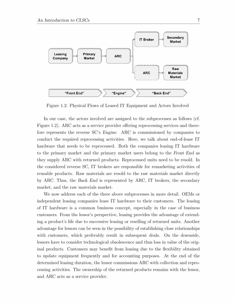
Figure 1.2: Physical Flows of Leased IT Equipment and Actors Involved
In our case, the actors involved are assigned to the subprocesses as follows (cf.
Figure 1.2). ARC acts as a service provider offering reprocessing services and there-
fore represents the reverse SC’s Engine. ARC is commissioned by companies to
conduct the required reprocessing activities. Here, we talk about end-of-lease IT
hardware that needs to be reprocessed. Both the companies leasing IT hardware
to the primary market and the primary market users belong to the Front End as
they supply ARC with returned products. Reprocessed units need to be resold. In
the considered reverse SC, IT brokers are responsible for remarketing activities of
reusable products. Raw materials are resold to the raw materials market directly
by ARC. Thus, the Back End is represented by ARC, IT brokers, the secondary
market, and the raw materials market.
We now address each of the three above subprocesses in more detail. OEMs or
independent leasing companies lease IT hardware to their customers. The leasing
of IT hardware is a common business concept, especially in the case of business
customers. From the lessor’s perspective, leasing provides the advantage of extend-
ing a product’s life due to successive leasing or reselling of returned units. Another
advantage for lessors can be seen in the possibility of establishing close relationships
with customers, which preferably result in subsequent deals. On the downside,
lessors have to consider technological obsolescence and thus loss in value of the orig-
inal products. Customers may benefit from leasing due to the flexibility obtained
to update equipment frequently and for accounting purposes. At the end of the
determined leasing duration, the lessor commissions ARC with collection and repro-
cessing activities. The ownership of the returned products remains with the lessor,
and ARC acts as a service provider.
An Introduction to CLSCs 8
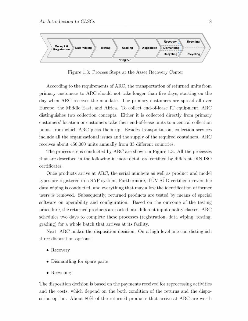
Figure 1.3: Process Steps at the Asset Recovery Center
According to the requirements of ARC, the transportation of returned units from
primary customers to ARC should not take longer than five days, starting on the
day when ARC receives the mandate. The primary customers are spread all over
Europe, the Middle East, and Africa. To collect end-of-lease IT equipment, ARC
distinguishes two collection concepts. Either it is collected directly from primary
customers’ location or customers take their end-of-lease units to a central collection
point, from which ARC picks them up. Besides transportation, collection services
include all the organizational issues and the supply of the required containers. ARC
receives about 450,000 units annually from 33 different countries.
The process steps conducted by ARC are shown in Figure 1.3. All the processes
that are described in the following in more detail are certified by different DIN ISO
certificates.
Once products arrive at ARC, the serial numbers as well as product and model
types are registered in a SAP system. Furthermore, TUV SUD certified irreversible
data wiping is conducted, and everything that may allow the identification of former
users is removed. Subsequently, returned products are tested by means of special
software on operability and configuration. Based on the outcome of the testing
procedure, the returned products are sorted into different input quality classes. ARC
schedules two days to complete these processes (registration, data wiping, testing,
grading) for a whole batch that arrives at its facility.
Next, ARC makes the disposition decision. On a high level one can distinguish
three disposition options:
• Recovery
• Dismantling for spare parts
• Recycling
The disposition decision is based on the payments received for reprocessing activities
and the costs, which depend on the both condition of the returns and the dispo-
sition option. About 80% of the returned products that arrive at ARC are worth

An Introduction to CLSCs 9
recovering and reselling on the secondary market. In the case of recovery, input-
quality-dependent reprocessing steps are conducted to bring the returns to an output
quality level that can be resold. ARC distinguishes different output quality levels,
for example depending on the technology standard. The required recovery activities
include cleaning, repair, installation of software, asset upgrading, and packing. To
conduct recovery activities, ARC schedules a total of five days for the completion of
one batch.
On behalf of its customers, ARC sells recovered IT equipment to an established
group of IT brokers, who are then responsible for remarketing activities. Reprocessed
products are sold in batches, rather than in individual units. When creating these
batches, several aspects need to be considered. Brokers are interested in batches that
include many homogeneous products. This is due to the savings in transportation
costs as well as the experience that homogeneous batches can be sold more easily
to secondary customers. From the seller’s perspective, the depreciation of recovered
units during the waiting time to achieve a certain amount of products needs to be
considered. Furthermore, the broker’s reselling network and its saturation need to
be taken into account when thinking of the amounts within a batch. Currently, ARC
arranges fixed prices for certain output quality levels with the brokers with whom
they usually work. Commonly, the batches include about 200 units. Furthermore,
it is ensured that all the recovered equipment is bought by one of the brokers in
ARC’s network.
If a given return is not worth recovering, it is dismantled and the reusable parts
are sorted out and stored. About 110,000 reusable parts, such as graphics cards or
storage components, are obtained annually from dismantling. These reusable parts
are used as spare parts in the recovery process. Everything else is recycled. In the
case of ARC, this amounts to a volume of about 3.5 t per year. The composition of
the materials actually included is not specified further.
We now turn to the back end of the reverse SC shown in Figure 1.2. Depending
on the disposition decision and successive reprocessing activities, two redistribution
channels are distinguished: reselling and recycling. We start with the reselling chan-
nel. As mentioned above, ARC uses authorized IT brokers instead of selling directly
to secondary end customers. A common role of such IT brokers is to buy recovered
equipment and resell it to the secondary market. Motivated by the decreasing mar-
gins that are achievable on the secondary market, lately, more and more IT brokers
have extended their business portfolio. One method is to offer service packages in-
cluding the installation of IT hardware and support issues. This represents an offer
that is especially attractive to smaller companies that do not employ special IT

An Introduction to CLSCs 10
staff. An alternative extension to the IT broker business is to conduct reprocessing
services. Hence, they become direct competitors to reverse logistics service providers
such as ARC.
Here, IT equipment is returned after the end of the leasing duration of usually
three years. This results in considerable depreciation in the IT hardware sector,
and reprocessed IT hardware cannot be sold “as new”. According to Atasu et al.
(2008), reprocessed products are attractive to the functional and green customer
segments. While functional-oriented customers value the function of a product over
its newness, the main driver of environmentally conscious customers to buy repro-
cessed products is waste reduction. Therefore, the focus is on functional and green
customers. Furthermore, the market consists of private and business customers; in
the case of the latter, the company size plays an additional role. According to ARC,
the recovered units are resold exclusively to business customers by the IT brokers.
The recycling of materials represents the second redistribution channel. Products
that are not worth recovering and their parts that cannot be used as spare parts are
recycled. ARC sorts these components according to 83 different materials and sells
them directly to the raw materials market. IT hardware contains valuable elements,
such as gold, silver, and copper, as well as different rare earth metals. As the value
of these materials is expected to increase in the future, the recycling of IT hardware
is seen as a profitable option.
In this chapter, we introduced an example of a reverse SC for end-of-lease IT
equipment by focusing on the reverse logistics service provider ARC. We provided
an overview of how the processes work at ARC and how it is linked to other actors
in the considered reverse SC.
Why does this setting attract our attention? First, the SC structure described
extends the previous literature by specifically addressing the role of a service provider
responsible for the reprocessing activities. Second, we consider a reverse SC con-
sisting of multiple, independent decision makers. Therefore, the described business
case represents an interesting basis on which to deduce the coordination needs in a
CLSC context.
1.4 Identified Research Needs
In Section 1.3, we introduced a service provider responsible for reprocessing activities
and the reverse SC of which this service provider is part. Due to the decentralized
setting, we concluded that there is a necessity to analyze CLSCs with regard to
potential coordination obstacles. The vast spectrum of decisions that may be con-

An Introduction to CLSCs 11
sidered in this context offers diverse research opportunities. Our choice for the focus
of this thesis is inspired by the major distinction between traditional SCs and CLSCs:
the heterogeneity of the supply side. The Heterogeneity of supplies originates from
the customers and their usage and return behavior. Hence, the link to the customers
represents one research project of this thesis. Further, the heterogeneity of the sup-
plies make the choice of appropriate reprocessing activities a necessity for profitable
reverse SCs. Thus, the disposition of returned products is another research project.
Both aspects are of special interest as they are CLSC-specific, and therefore open
up the possibility to provide new insights to the research on coordination in SCs.
The Case of the Disposition Decision
In the business case introduced, two actors are directly affected by the disposition
decision: the lessor and ARC. Currently, the lessor pays ARC to conduct repro-
cessing services and receives the revenues that are achievable on the secondary and
raw materials markets. These revenues in turn depend on the output quality level
achieved. This means that the lessor’s achievable revenues depend on ARC’s dispo-
sition decision. As we face a decentralized SC, this raises the question of whether a
coordination need exists with respect to the disposition decision.
This becomes even more interesting against the background of the distribution
of information on returns. Due to the chosen business model to lease IT hardware
to primary customers, the uncertainty with respect to the timing and quantity of
returns is relatively limited. However, quality uncertainty remains. In the current
setting, only primary customers and ARC have knowledge of the actual quality of
returns. The lessor, who owns the products and has to pay for reprocessing services,
is not able to observe the actual quality of its end-of-lease IT equipment. This is
because end-of-lease units are transported from primary customers directly to ARC
(cf. Figure 1.2).
While previous research on reverse or CLSC coordination needs focuses on the
OEM perspective (Savaskan et al., 2004; Savaskan and Van Wassenhove, 2006; Atasu
et al., 2013), the setting described here offers a new perspective that is becoming
more and more important. The increasing importance is due to two major factors.
First, companies focus on core competences, such as research and development, and
outsource the actual production. Consequently, they often lose know-how and are
not able to establish profitable reprocessing activities. Second, growing numbers of
leasing companies that are not OEMs are entering the market. These companies
are not involved in any production processes and therefore are not able to conduct
reprocessing activities on their own. Therefore, the reverse SC structure observed

An Introduction to CLSCs 12
in the business case is representative of other cases as well and worth addressing
in greater detail. We investigate the coordination of the disposition decision in
Chapter 3 and address the following research question:
How can the disposition decision be coordinated in the case of reverse
SCs consisting of multiple, independent actors?
The Customer Interface
The first research focus is supported by the fact that the information asymmetry
concerning the condition of returns may cause SC deficiency. As users of potential
product returns, customers commonly have exclusive knowledge about the condition
of products. Furthermore, end users have decision power regarding when to return
a product, if they intend to return it at all.
The value of information on the aforementioned uncertainties present in CLSCs is
analyzed by several authors (Ferrer, 2003; Ferrer and Ketzenberg, 2004; Ketzenberg
et al., 2006; De Brito and Van der Laan, 2009). However, the focus of previous
research, as well as the focus of industry practice, is on the operational aspects of
CLSCs (Guide et al., 2003), which take these uncertainties as exogenous. Besides
the market demand and technical feasibility of reprocessing activities, Geyer and
Jackson (2004) and Guide and Van Wassenhove (2009) identify the limited access
to supply and supply information as major obstacles to efficient reverse SCs. Since
then, three different concepts (which we will introduce later on) to reduce supply
uncertainty have been developed.
However, to the best of our knowledge, no research exists on customers and the
effects of their decisions on CLSCs’ process from a SC coordination perspective. To
close this gap, we address the following research question in Chapter 4:
Taking a holistic CLSC perspective, what are the needs for coordination
at the customer interface?
1.5 Outline of the Thesis
This thesis consists of five chapters. Chapter 1 represents the basis on which both
the research aim of this thesis and the actual research questions addressed in subse-
quent chapters are motivated. In Chapter 2, we embed this research focus into the
previous literature. An in-depth analysis of the identified coordination requirements
is provided in Chapters 3 and 4. We conclude this thesis in Chapter 5 by recapitu-
lating our results and pointing out future research directions. In the following, we

An Introduction to CLSCs 13
summarize the content of these chapters in more detail.
Chapter 1 is composed of four parts. In our introductory section, we highlight
the necessity to focus on decentralized CLSCs and the resulting research goals of
this thesis are stated. Subsequently, we provide an overview of the actors involved
in such a decentralized setting and the processes that are of relevance. The first
contribution of this thesis is the introduction of the ARC business case. On the one
hand, the case is a contribution to the literature itself, and on the other hand, we
derive concrete research needs based on the decentralized setting.
Chapter 2 provides an overview of the previous research on coordination both in a
forward SC context and in a CLSC context. Based on the comparison of managerial
requirements observed in the business case and the academic literature, we identify
gaps that are addressed within the further analysis chapters of this thesis.
In Chapter 3, the coordination of the reverse-SC-specific process step “disposi-
tion” is addressed. To this end, we compare the introduced business case setting
with our benchmark, a central decision maker. We see that the current setting re-
sults in a suboptimal CLSC solution. To overcome this SC deficiency, we develop a
coordinating mechanism. Beyond the analysis, we provide a numerical example to
illustrate our insights.
CLSCs are characterized by heterogeneous supplies with respect to quality, quan-
tity, and timing. The increase in supply uncertainty originates from the customer’s
use phase, which in many cases is a kind of “black box” for the other actors in
CLSCs. In Chapter 4, we address customer decisions and identify the coordination
needs resulting from these decisions. Furthermore, we discuss the adaptability of
existing mechanisms to the coordination requirements at the customer interface.
Finally, in Chapter 5, we summarize our findings and present the directions for
future research.
Chapter 2
Coordination of Multiple Decision
Makers - Structuring the Field
In this chapter, the identified coordination issues considered in this thesis are em-
bedded into the previous literature. Coordination has been studied extensively in
traditional SCM; therefore, we start this review with an overview of the literature on
coordination issues in the case of multiple, independent decision makers in forward
SCs (Section 2.1). The aim is to provide an overview of the developed coordination
mechanisms on which we can build in our analysis chapters (Chapters 3 and 4). Sub-
sequently, we review the previous literature on coordination in CLSCs (Section 2.2)
and highlight our contributions to this research stream.
2.1 Coordination in the Forward Supply Chain
Literature
Unaligned incentives as well as information asymmetries of the parties involved in
decentralized SCs are identified as major obstacles to efficient SCM. Therefore, co-
ordination “is perceived as a prerequisite to integrate operations of supply chain
entities to achieve common goals” (Arshinder et al., 2011, p.44). The goal of coordi-
nation commonly is to achieve SC-wide optimality with respect to profit maximiza-
tion or cost reduction (Tsay et al., 1999). Coordination takes a central role in the
management of SCs and spans multiple directions (Ballou et al., 2000). On the one
hand, one has to distinguish between intra-organizational and inter-organizational
coordination. While the first concerns the coordination of activities like logistics,
accounting, and marketing within one organization, the latter concerns the coordi-
nation of legally independent organizations. On the other hand, one can distinguish
14
Coordination of Multiple Decision Makers - Structuring the Field 15
between vertical and horizontal coordination - coordination along the SC or coordi-
nation between organizations at the same stage of the SC.
In the following, the mechanisms to achieve coordination are introduced. The
mechanisms found in the previous literature address either settings in which coordi-
nation is hampered due to unaligned incentives (Section 2.1.1) or settings suffering
from both unaligned incentives and information asymmetries (Section 2.1.2).
2.1.1 How to Coordinate Actions in Decentralized Supply
Chains
To achieve optimal SC performance, certain actions are required. However, these
SC optimal actions often conflict with actors’ individual objectives. To match the
individual objectives with the SC objective, contracts defining transfer payments
have been introduced. In the following, we review the mechanisms coordinating the
order decision in SCs with unaligned incentives, under the assumption that there is
no information asymmetry between the actors involved. We close this section with
an overview of the extensions to this basic setting.
Mechanisms to Achieve Supply Chain Optimal Order Quantities
In the most basic setting for which contracts are developed, two risk-neutral actors
and a one-period time horizon are assumed: a single upstream party sells a product
to a single downstream party, which faces the so-called newsvendor problem. In
a newsvendor setting, the demand for a certain product is stochastic and only one
ordering opportunity exists well in advance of the actual selling season. Products can
be used to satisfy the demand of one selling season only. Thus, the trade-off between
the risk of ordering too much and the risk of ordering too little has to be considered
when determining the optimal order quantity. “Optimal” is hard to define here as
the demand is uncertain. A usual performance measure is the expected profit.
The analyzed SC consists of a supplier and a retailer. In the basic setting, it
is assumed that both actors have access to all the relevant information. Although
common in practice, a wholesale price contract does not coordinate this setting due
to double marginalization. Incentives are needed to make the retailer order the SC
optimal quantity1 q◦. It is shown that this can be achieved by several contracts:
buyback, revenue-sharing, quantity-flexibility, sales-rebate, and quantity-discount
contracts. Cachon (2003) provides an excellent overview of SC coordination with
contracts. The following introduction to the aforementioned contracts coordinating
1Notation is taken from Cachon (2003)

Coordination of Multiple Decision Makers - Structuring the Field 16
the basic setting is based on this commonly cited chapter. Thereby, we focus on the
general, underlying mechanisms. For a more detailed analysis of contract structures,
we refer the interested reader to Cachon (2003).
Buyback and revenue-sharing contracts are proven to be equivalent in the basic
setting. Under a buyback contract, the supplier charges a wholesale price wb per
unit, but additionally a second parameter is part of the contract: a certain amount
b is paid per unsold unit at the end of the selling season, with b ≤ wb. Applying a
revenue-sharing contract results in a reduced wholesale price wr ≤ w. In addition
to the wholesale price, the retailer pays an agreed fraction 1 − φ of his achieved
revenue to his supplier. Hence, in both cases, the retailer is refunded in the case
that the actual demand is below the ordered quantity, a mechanism that (Cachon,
2003, p.255) refers to as “downside protection”.
A quantity-flexibility contract also works by the “downside protection” mecha-
nism. However, the structure differs from the aforementioned contracts. A quantity-
flexibility contract consists of two components: the wholesale price wq, which is
charged for each ordered unit, and a refund, which the retailer receives at the end
of the selling season according to the following scheme: (wq + cr − salvage value) ∗min{leftover units; δ ∗ q}, with contract parameter δ ∈ [0, 1]. “Hence, the quantity-
flexibility contract fully protects the retailer on a portion of the retailer’s order
whereas the buyback contract gives partial protection on the retailer’s entire order”
(Cachon, 2003, p.248). A further distinction is that in contrast to the buyback and
revenue-sharing contracts, the quantity-flexibility contract is not assured to result
in SC coordination under voluntary compliance.
One can distinguish between forced and voluntary compliance. While forced
compliance assumes that exactly the amount ordered is delivered due to sufficiently
hard consequences, under voluntary compliance the supplier delivers the amount
that results in the maximum profits for him (but not more than the ordered quan-
tity).
A sales-rebate contract consists of three parameters: the wholesale price ws, the
rebate r, and the threshold t. The retailer pays ws as long as the ordered amount
is below the threshold. If q ≥ t, the retailer has to pay a reduced wholesale price
ws−r for all the ordered units plus a rebate for the first t units and for all the unsold
units above t. Here, so-called “upside protection” is given. For any unit sold above
t, the retailer pays less than the production cost. A sales-rebate contract does not
coordinate SCs under voluntary compliance.
Diverse quantity-discount contracts are proposed in the literature. In general,
coordination can be achieved due to manipulation of “(. . . ) the retailer’s marginal

Coordination of Multiple Decision Makers - Structuring the Field 17
cost curve, while leaving the retailer’s marginal revenue untouched” (Cachon, 2003,
p.254).
Extensions
The extensions to the basic model cover two directions: either the optimal order
quantity is considered in different settings or an additional decision is taken into
account.
Kouvelis and Lariviere (2000) introduce the alternative setting in which the
set of transfer payments is not fixed but determined via internal markets after the
relevant information has been revealed. The authors show that such internal markets
coordinate the SC as well. Donohue (2000) introduces a setting with two ordering
opportunities. Here, the optimal order quantity of the first order (before the early
demand is observable) and the optimal second order quantity (after the early demand
has been observed) need to be incentivized. Alternatively, the considered “one-to-
one” SC structure is changed. Cachon (2003) describes and extends contracts for
the optimal order quantity with multiple retailers (“one-to-many”). Cachon and
Kok (2010) introduce a SC consisting of competing manufacturers and one single
retailer (“many-to-one”). On this line, Li et al. (2013) analyze the contract choice
in the case of competition between multiple retailers as well as between multiple
manufacturers. Ha and Tong (2008) analyze the optimal contract design in the
case of two competing “one-to-one” SCs. Recent research effort also points in two
further directions: Feng and Lu (2013) introduce bilateral bargaining instead of the
common Stackelberg game, and Chen et al. (2014) analyze the question of stability
of contracts in the case of the involvement of risk-averse actors.
Furthermore, besides the pure consideration of order quantity, the coordinating
contracts found in the literature jointly specify different parameters, like retail prices,
time, or quality. We refer to Arshinder et al. (2011) for a summary.
In sum, three different contract types (downside protection, upside protection,
and quantity discounts) are introduced to coordinate the basic setting (thus, making
the retailer order the SC optimal order quantity). Some of these contracts are
reported to coordinate extensions of the basic setting as well - either in their pure
form or as combinations.
The contracts differ with respect to the cost of administration, the distribu-
tion/shifting of risk between the actors involved and the information required to
choose the contract parameters. These factors may indicate which contract is the
best match in different real-world situations and need to be checked when transfer-
ring the contracts to alternative settings.

Coordination of Multiple Decision Makers - Structuring the Field 18
2.1.2 How to Coordinate Actions and Pursue Information
Transfer in Decentralized Supply Chains
An underlying assumption of the aforementioned models is that all the actors have
access to all the available and required information. However, this is not always
the case. Information with respect to the demand, exerted selling effort, inventory
position, or inventory control policy that is in place (so-called “downstream infor-
mation”) and information with respect to cost structures, lead time, or capacity
(“upstream information”) may be scattered among diverse actors. Therefore, in the
case of asymmetric information, besides the coordination of actions, the sharing of
accurate information needs to be pursued (Chen, 2003).
In such settings, the idea of the agency literature2 is often applied. Depend-
ing on whether the principal or the agent is offering the contract, the concepts of
screening and signaling are distinguished. Besides contracts, collaborative initiatives
to coordinate such SC settings are found in the literature. The following overview
of the literature dealing with the exchange of information in decentralized SCs is
structured accordingly.
Screening
The objective of screening models is to design contracts that provide incentives to
gather the private information held by one SC entity. The action to coordinate is
the order quantity.
Information asymmetry on an actor’s cost structure represents one research di-
rection within this stream. Corbett and De Groote (2000) consider a retailer’s
holding cost parameter that is unknown to the supplier. They derive the optimal
quantity discount policy to make the buyer order the SC optimal quantities. Ha
(2001) and Corbett et al. (2004) consider supplier-buyer relationships under infor-
mation asymmetry with regard to the buyer’s cost structure. Ha (2001) shows the
optimality of “a cutoff policy on the buyers marginal cost to determine whether a
contract should be signed” (p.43). The optimal cutoff level is affected by both the
supplier’s marginal costs and the buyer’s reservation profit. Corbett et al. (2004)
compare different contract types in the case of full and asymmetric information.
One of their major findings is that the “value of information is greater under two-
part contracts than under one-part contracts, and the value of being able to offer
two-part contracts rather than one-part contracts is greater under full information
than under asymmetric information” (p.558).
2An introduction to the principal-agent theory is provided by Kreps (1990)

Coordination of Multiple Decision Makers - Structuring the Field 19
Private demand information is the second research direction considered in the
previous literature (e.g. Lariviere, 2002; Ozer and Wei, 2006). Lariviere (2002)
considers a SC consisting of a supplier and a retailer facing the newsvendor prob-
lem. The demand information is likely to be improved due to costly forecasting
by the retailer. The supplier wants to induce the retailer to forecast and to share
this information with him. However, the supplier cannot observe the retailer’s fore-
casting activities. The authors examine and compare the performance of buyback
and quantity-flexibility contracts in this regard. They conclude that the perfor-
mance depends on the costs of forecasting. In the case of high forecasting costs, the
quantity-flexibility contract is preferred (and vice versa). Ozer and Wei (2006) show
that a non-linear price capacity reservation contract results in credible information
sharing and profit maximization. Ha and Tong (2008) consider two one-to-one SCs
and analyze “how the incentive contracts change under different information struc-
tures in a competitive environment” (p.703).
Besides the aforementioned information on the demand and cost structure, the
decision on exerted selling effort is usually known only by the responsible actor, that
is, the retailer. Higher selling effort, thus increased demand, is beneficial to both
actors but only costly to the retailer. An intuitive solution is to share the costs
occurring between the two actors, but the actual effort may be hard to monitor by
the supplier and sometimes not only one supplier benefits from the retailer’s selling
efforts. Thus, direct transfer payments are not possible (Porteus and Whang, 1991).
Cachon (2003) shows that buyback, revenue-sharing, and quantity-flexibility con-
tracts result in less effort than is SC optimal, whereas a sales-rebate contract leads
to too much effort. A combination of the sales-rebate and buyback contracts can
solve this problem and result in the optimal SC effort, but as many as four different
parameters are required to implement this combination. Besides this combined con-
tract, the quantity-discount contract leads to SC optimal effort and order quantity
decision. It is not only the demand that can be influenced by the exerted efforts.
Several papers (e.g. Reyniers and Tapiero, 1995; Baiman et al., 2000) analyze the
influence of the chosen effort on the resulting quality of the delivered products,
whereas Wang and Shin (2013) consider the innovation effort and its effects on cus-
tomers’ product valuation.
Signaling
The objective of an informed entity in transferring its private information to an
uninformed one is known as signaling. Interestingly, signaling is mostly used in the
context of new product introduction (Chen, 2003). The models assume that man-

Coordination of Multiple Decision Makers - Structuring the Field 20
ufacturers introducing a new product usually possess superior information on the
market demand. This information is shared either with downstream SC partners,
such as retailers, or with upstream partners, such as suppliers. Papers like Chu
(1992), Desai and Srinivasan (1995), or Lariviere and Padmanabhan (1997) address
signaling games between well-informed manufacturers and retailers. The underlying
problem is to convince the uninformed retailer to carry the product, although this
incurs costs and overstocks may not be returnable. With respect to upstream part-
ners, Cachon and Lariviere (2001) investigate the issue that manufacturers need to
convince their supplier(s) to build up sufficiently large capacities.
Coordination by Joint Decision-Making Initiatives
Joint decision-making initiatives represent another set of mechanisms to achieve SC
optimal actions under information asymmetry (Arshinder et al., 2011). The basis
of all of them consists of information and communication technology (ICT) tools.
In the following, the most common initiatives are introduced, sorted by increasing
collaboration effort and the degree of information sharing required.
Quick Response is an inventory management initiative that originates from the
apparel industry. The underlying idea is that lead times are shortened and retailers
can therefore order closer to the actual selling season and thus based on a better
forecast. Nevertheless, certain actions, such as service level or volume commitments,
are required to make both actors better off than without Quick Response (Iyer and
Bergen, 1997).
Collaborative Planning, Forecasting, and Replenishment means that the SC part-
ners share information and work closely together in their core SC business processes
(Aviv, 2001). Among other benefits, increased sales, better service levels, and re-
duced capacity requirements are mentioned in the literature. A road map showing
how to achieve these objectives is offered by the Voluntary Interindustry Commerce
Standard Association (1999). Subsets of this standard set of technology-enabled
business processes, like collaborative forecasting, are discussed in the literature as
well (e.g. Aviv, 2001, 2007).
Vendor Managed Inventory (VMI) is a further technology-enabled mechanism
to achieve optimal decision making within a SC. If VMI is in place, the timing
and quantity of the reordering decision is shifted from the retailer to the supplier
(Aviv and Federgruen, 1998). The basic requirement of a VMI system is that the
demand and inventory information is shared within the SC. Furthermore, ICT is
required to enable real-time and accurate transmission. A major advantage of VMI
for suppliers is the possibility to overcome the bullwhip effect (Disney and Towill,
Coordination of Multiple Decision Makers - Structuring the Field 21
2003). On the retailer side, ordering and inventory monitoring cost savings are
often highlighted. Mishra et al. (2009) argue that such savings are possibly realized
already by the introduction of technology like electronic data interchange systems,
hence looking for an alternative explanation for why retailers often “force” their
supplier to install a VMI system. They show that the competition between suppliers
of product substitutes is intensified by VMI. Retailers benefit from this increased
competition, which the authors take as reasoning for the observed popularity of VMI
among retailers.
Summarizing the literature on the coordination of forward SCs, Arshinder et al.
(2011) state, “(. . . ) literature has emphasized more on demand uncertainty, whereas
supply uncertainty can be of equal concern in the era of globalization and outsourc-
ing” (p.67). This circumstance may complicate the transferability of the developed
mechanisms to a CLSC context, in which supply uncertainty represents a major
challenge. Nevertheless, the mechanisms introduced in this section may be useful as
a starting point and can be drawn on in this thesis.
2.2 Coordination in the Closed-Loop Supply
Chain Literature
The vast majority of the literature in CLSC research addresses technical and oper-
ational issues (Guide and Van Wassenhove, 2009). A common assumption is that
the planning of the CLSC processes, such as scheduling and shop floor control,
inventory management, or network planning, is undertaken by a central planner.
Ferguson (2009) and Souza (2013) provide recent reviews of previous publications
in this literature stream.
The focus of this section is on the literature modeling the issues arising from mul-
tiple, independent decision makers in CLSCs with non-aligned objectives. Thierry
et al. (1995) are among the first to transfer the necessity to take multiple decision
makers into account in a CLSC setting. Studying the product recovery management
of an international copier manufacturer, BMW, and IBM, one of their key findings
is that it is important to cooperate with other organizations in one’s reverse (or even
better closed-loop) SC. According to the authors, cooperation opportunities include
working with companies that specialize in product reprocessing activities as well as
joint product redesign.
In line with Savaskan et al. (2004), we distinguish two “clusters” of resulting
research efforts on the strategic interaction among CLSC actors. We start with the

Coordination of Multiple Decision Makers - Structuring the Field 22
literature on the reverse channel structure for collection and the literature on false
failure returns. Both coordination issues occur ex post, that is, they are related
to the after-usage phase. Finally, we address product-design-related issues, which
occur ex ante.
Reverse Channel Structure for Collection
The general idea of this research stream is to obtain a detailed understanding of the
implications that a manufacturer’s reverse channel choice has for forward channel
pricing decisions and for the collection rate, specifically how the profits are affected.
To make collection economically beneficial, it is assumed that the production of
new products is cheaper in the case that returned products are used instead of new
supplies. Linked to this assumption, it is assumed that returned products are of
homogeneous quality.
Savaskan et al. (2004) consider a two-echelon SC consisting of a single manu-
facturer and a single retailer. The manufacturer can choose between three different
reverse channel structures: (1) the manufacturer collects returns directly from cus-
tomers, (2) the retailer is responsible for the collection, and (3) a third party is
commissioned with the collection of product returns. These decentralized settings
are compared with a central decision maker in terms of wholesale price, retail price,
product return rate, and total SC profit. All the settings are modeled as Stackelberg
games, with the manufacturer as the Stackelberg leader.
The analysis shows that in the case that prices are sensitive to changes in the unit
production costs, the best option is to choose the retailer to collect used products.
This choice results in the highest collection rate, the lowest retail price, and thus
the highest sales volumes. This consequently results in the best SC profit in a
decentralized setting. Furthermore, it is shown that the profits of both actors,
manufacturer and retailer, increase in comparison with the alternative settings. The
authors explain their result in the following way. The amount of potentially collected
products is limited by the sales volume of the first period. As the retail price affects
the sales volume, it is seen as the main driver in this model. In the case that a
retailer takes into account the future benefits from the collected products, he is able
to decrease his retail price. Due to the lower retail price, the sales volume increases,
from which the manufacturer benefits as well - hence, he is able to offer a decreased
wholesale price to the retailer. This effect is observable only to some extent in
the case that the manufacturer collects the products. Again, the production costs
are lowered due to the usage of returned products, but these savings will not be
transferred completely in terms of a reduced wholesale price. This problem is known
Coordination of Multiple Decision Makers - Structuring the Field 23
from traditional SCM coordination as double marginalization (Spengler, 1950). The
third-party option is the least preferred one as again the double marginalization
problem arises. Additionally, the SC profits are decreased due to the payments for
the collection activities of the third party. Furthermore, the authors show that as a
result of the introduction of a two-part tariff, the retailer collection setting leads to
SC optimal profits, obtained by a central planner. However, this assumes complete
information on the costs as well as the demand.
Savaskan and Van Wassenhove (2006) extend the above model of a single man-
ufacturer-retailer dyad by incorporating competing retailers. The authors analyze
five different reverse channel structures: on the one hand, decentralized settings with
(1) no collection at all, (2) returns are collected directly from the manufacturer, (3)
retailers being responsible for the collection; and on the other hand, two centralized
settings with (4) direct collection and (5) indirect collection via retailers. Using a
game theoretic modeling framework, they provide insights into how wholesale prices
and the retailer’s intensity of competitive behavior are affected by the reverse channel
structure. In the case of competing retailers, the manufacturer’s optimal choice
depends on the product under consideration. In the case of consumer products,
that is, when retailers compete on prices, the indirect, retailer collection is the
best option. If the retailers cannot affect the prices, or only to a small extent,
manufacturer collection is preferred.
Atasu et al. (2013) provide another extension to the model of Savaskan et al.
(2004) by incorporating volume-dependent costs. Depending on the environment in
which a company operates, two different collection cost structures are distinguished.
A company faces either economies of scale in the collection cost, for example due to
the quantity discounts of a mail provider, or diseconomies of scale, which relate to
settings in which more distant (thus more expensive) customers need to be reached
to increase the collection volume. Similar to the result of Savaskan et al. (2004),
retailer collection is the manufacturer’s optimal choice in the case that the retailer
is incentivized to increase the sales volume. This is achieved either due to the
above scale effect in investment costs or due to economies of scale in collection
costs. Otherwise - such as in the case of diseconomies of scale - manufacturer
collection is preferred. Again, third-party collection is always dominated. While this
differentiation according to costs is not too surprising, the major contribution of this
paper is to show that the analysis of the collection cost structure is of importance
for the optimal reverse channel structure choice.
Karakayali et al. (2007) focus on a CLSC setting motivated by the automotive
industry. OEMs are often obligated by law to fulfill certain recycling targets. How-

Coordination of Multiple Decision Makers - Structuring the Field 24
ever, due to disappointing experiences, they tend to outsource these activities. To
model this decision, a SC consisting of a collector and a reprocessor is considered. In
contrast to the aforementioned papers, the authors include heterogeneous qualities
of returned products. The collecting actor decides on the quality-dependent acqui-
sition price for the used products. The reprocessing actor decides on the amount of
products that are remanufactured, pays a transfer price to the collector, and deter-
mines the reselling price. The authors analyze how the pricing decisions of agents
responsible for the collecting or processing of end-of-life product returns influence
the collection rate. As a benchmark, they introduce a central decision maker respon-
sible for both collection and reprocessing. Two decentralized settings are compared
with this benchmark: either the collector or the reprocessor is modeled as the Stack-
elberg leader. It is shown that a two-part tariff consisting of a quality-dependent
unit wholesale price and a fixed payment coordinates both decentralized settings.
False Failure Returns
While the aforementioned models address returns that have been used by customers
for a longer period of time, Ferguson et al. (2006) consider false failure returns, that
is products that are returned by customers although they do not have any functional
or cosmetic disfunctionalities. According to the authors, most returns of this type
could be avoided due to increased sales efforts. However, these efforts need to be
taken by the retailers, while the manufacturer benefits from them as he can save
the costs incurred by the reverse flows. To coordinate the setting, the authors in-
troduce a target rebate contract. This means that the manufacturer pays a certain
amount per unit of false failure return below a target value to the retailer. Due to
the payment, the retailer has the incentive to exert sales effort, thereby decreasing
the amount of false failure returns and thus the decreasing reverse SC costs for the
manufacturer.
Product Design
A precondition of the above considerations is the reusability of a product. Reusabil-
ity is a central product design decision and is related to further CLSC processes and
actors. The production of reusable products usually is more expensive than the pro-
duction of a single-use product (Debo et al., 2005). However, reusable products can
be recovered at lower costs than the initial production costs (e.g. Ferguson, 2009).
The most fundamental question that has to be answered is whether reusability of a
product is profitable.
Debo et al. (2005) address this question under the assumption of heterogeneous

Coordination of Multiple Decision Makers - Structuring the Field 25
customers. Customers differ from each other in terms of high and low degrees of
willingness to pay for a new product as well as heterogeneity with respect to the
willingness to pay for reprocessed products - whereas new and reprocessed prod-
ucts are substitutes, but reprocessed products are valued less than new ones. As
key drivers of an increasing reusability level, the authors identify decreasing repro-
cessing costs as well as decreasing incremental costs associated with producing a
reusable product instead of a single-use one. Besides costs structures, the choice of
reusability is driven by the customer structure: “the optimal remanufacturability
level is the highest for medium levels of market heterogeneity. For markets with
high concentrations of customers on either the high end or the low end, the opti-
mal remanufacturability level is low”(p.1200). Hence, knowledge of the customer
structure is central when determining attributes like reusability.
The coexistence of new and reprocessed products is briefly covered by the au-
thors. The focus is consequently on the special role of new products. Their results
indicate that the “practice of focusing on the profits obtained from new and reman-
ufactured products separately can be counterproductive, and that considering the
total product line as part of the same profit center may lead to higher profitability
for the firm”(p.1201).
The reusability potentially offers the opportunity for independent reprocessing
companies to enter the market. Therefore, competition with independent repro-
cessors also needs to be considered when deciding on the level of reusability. In
this regard, the authors find that the key drivers for the introduction of a reusable
product remain. However, the level of reusability decreases with the number of
competitors.
Geyer et al. (2007) analyze several aspects that potentially influence the cost
savings obtained from reprocessing activities besides the product design. Their result
highlights the necessity to consider simultaneously the production cost structure,
collection rate, product life cycle, and component durability. This is a very complex
task that - according to the authors is possibly an explanation for why many OEMs
avoid closing the loop.
To summarize, it can be stated that the research on coordination in CLSCs is
still in an early stage. We contribute to this stream of research in multiple ways:
• Due to the introduction of a business case the necessity of coordination in the
CLSC context is highlighted.
• The literature on the optimal reverse channel structure is extended by our
analysis of the coordination of the disposition decision in a decentralized CLSC.

Coordination of Multiple Decision Makers - Structuring the Field 26
• The analysis of the customer interface adds a new layer to the research on the
coordination of CLSCs. Customers as the origin of supply uncertainties are
analyzed in more detail and the effects of their decisions on CLSC processes
are considered from a coordination perspective.

Chapter 3
Coordination in Closed-Loop
Supply Chains - The Case of the
Disposition Decision
So far, the foundations for coordination issues in CLSCs have been laid. In this chap-
ter, we focus on one specific coordination aspect: the coordination of the reverse-SC-
specific process step disposition and related decisions. The main driver of this focus
is the business case introduced. We consider a decentralized reverse SC consisting
of a lessor and a service provider that conducts the reprocessing activities of end-
of-lease returns. The disposition decision affects the profits of both actors involved.
However, the essential information for the disposition decision - the information on
the actual quality of the returned products - is available only to the service provider.
Hence, decentralized decision making and scattered information between multiple
SC members raise the question of appropriate SC coordination with regard to the
disposition decision. Furthermore, the coordination of the disposition is of inter-
est as there is no obvious corresponding process step in a traditional forward SC.
Specifically, we address the research question raised in Section 1.4:
How can the disposition decision be coordinated in the case of reverse
SCs consisting of multiple, independent actors?
The chapter is structured as follows. In Section 3.1, a review of the relevant
literature on the disposition decision is provided, followed by the statement of as-
sumptions and the notation used (Section 3.2). The actual analysis of the identified
coordination need starts with the introduction of our benchmark - following the
standard SCM literature, we use a central decision maker who owns all the relevant
information (Section 3.3.1). The current business case setting is analyzed in Sec-
27

The Case of the Disposition Decision 28
tion 3.3.2. As it is shown not to be optimal, a coordinating strategy is developed
in Section 3.3.3. We illustrate the aforementioned settings in terms of an example
(Section 3.4) and conclude with a discussion of the assumptions and future research
directions (Section 3.5).
3.1 Literature Review - Disposition Decisions in
Closed-Loop Supply Chains
The main distinction between reverse SCs and traditional ones is the uncertainty
on the supply side with respect to the quantity, timing, and quality of returns
(Fleischmann et al., 2010). This is why the inbound processes, namely product
acquisition, grading, and disposition are of special interest in CLSC settings. In
our business case, we identified a potential SC deficiency with respect to one of
these inbound processes: the disposition decision. In this chapter, we characterize
the disposition decision (Section 3.1.1) and provide an overview of the previous
literature on the disposition decision (Section 3.1.2).
3.1.1 Characterizing the Disposition Decision
The objective of the disposition decision is to choose the most suitable disposition
option for returned products of a certain category. In the following, we summarize
the commonly distinguished categories of return flows and disposition options. In
the section on objectives, we state the basis for the choice of the most suitable dis-
position decision.
Categories of Return Flows
Heterogeneity of supplies makes it necessary to assess the condition of returned
products to be able to determine a suitable disposition option (Guide et al., 2000).
However, to some extent, information on the quality of supplies can be gathered even
without actually assessing the returned products. This is due to the different kinds
of return flows that exist. Three different categorization schemes of reverse flows
can be found in the literature. Thierry et al. (1995) are the first to mention return
types and their inherent different characteristics. Using the terminology of Guide
and Van Wassenhove (2009), three return types are distinguished: consumer returns,
end-of-use, and end-of-life. Consumer returns are products that are returned by end
customers due to dissatisfaction within a short period of time after the purchase.
This return type is usually hardly used and requires quick reintroduction into the

The Case of the Disposition Decision 29
market. End-of-use returns, such as leasing returns, are often attractive for a second
usage phase, whereas end-of-life returns are usually worn out and outdated with re-
spect to their technology. Guide and Van Wassenhove (2001) propose a distinction
between waste-stream and market-driven flows. Alternatively, Rogers et al. (2002)
introduce a categorization according to the origin of the product flow. Based on
information from the Global Supply Chain Forum, they distinguish five different
return flows: consumer returns (including returns due to defects as well as com-
mercial return policies), marketing returns (from a forward SC actor), asset returns
(transportation equipment, such as containers), product recalls, and environmental
returns.
Different return types and/or origins of return flows have an impact on the condi-
tion of returned products. Nevertheless, both the availability and the actual quality
are uncertain ex ante.
Disposition Options
Next, we come to the clarification of possible disposition options. Thierry et al.
(1995) are the first to provide an overview of observable disposition options. The
authors divide the different options into three groups: direct reuse, product recov-
ery, and waste. This common categorization is used in the following to describe
the diverse disposition options described in the previous literature in more detail.
Figure 3.1 provides a summarizing overview.
Let us start with the direct reuse options. Returned products that are in an “as
new” condition, for example consumer returns, can usually be resold directly or after
repacking. These products are sold for the original or a discount price. Depending
on the condition of returned products, further direct reuse alternatives are to sell
the products via an outlet to a secondary market or to donate them (Rogers and
Tibben-Lembke, 1998).
Product recovery covers disposition options that require “(...) a value-added op-
eration that restores a used product to a common operating and aesthetic standard,
and where the core geometry of the product is preserved” (Souza, 2012, p.150).
Commonly three disposition options are related to this group: repair, refurbishing,
and remanufacturing. These disposition options differ from each other in terms of
the degree of disassembly and the achieved quality level of the recovered product. To
repair a product, limited disassembly is usually required and due to a lower quality
level than a new product, repaired products cannot be sold “as new”. In contrast,
remanufacturing requires complete disassembly and inspection of the original prod-
uct to assure the quality standard of new products. Refurbishment is seen to be in

The Case of the Disposition Decision 30
Figure 3.1: Categorization of Disposition Options (based on Thierry et al., 1995)
between these two options. In addition to the aforementioned recovery alternatives,
Galbreth et al. (2013) recently addressed the option to include component upgrades
to cover technological innovations that evolved during the use phase of the product.
The disposition option disassembly for spare parts can be located in between
product recovery and waste. In contrast to the aforementioned recovery options,
in this option only a minority of components are reused. These components are,
depending on their inherent quality standard, used in the aforementioned recovery
processes (Thierry et al., 1995). In addition, Ferguson et al. (2011) observe that
spare parts can also be sold directly to customers. All other parts are disposed of
in some form. Recycling is another disposition option found in the literature. This
is the recovery of the materials of which a returned product consists. As in the case
of disassembly for spare parts, some materials are reintroduced in the forward SC,
whereas others are disposed of - but on a material instead of a component level.
In the literature, there are two disposition options that match Thierry et al.
(1995)’s waste category: incineration (i.e. energy recovery) and landfilling.

The Case of the Disposition Decision 31
Objectives
We introduced the choice of the most suitable disposition option for returned prod-
ucts as the objective of the disposition decision. This makes a definition of “most
suitable” necessary. The criteria can be summarized by the Triple Bottom Line
(Elkington, 1997):
• People, meaning social impact
• Planet, meaning environmental impact
• Profit, meaning economic goals
Although the focus of market-driven CLSCs is usually on profit maximization,
the prioritization of different aspects may vary depending on the decision maker
(Souza, 2012). Furthermore, multiple obstacles hamper straightforward decision
making, based on profit considerations. Besides the aforementioned supply uncer-
tainties, Fleischmann et al. (2010) as well as Souza (2012) highlight the following
complicating factors that should be taken into account to enable a good disposition
decision to be made:
1. Demand uncertainties. These includes uncertainties with respect to the de-
mand for reprocessed products as well as differences in the demand for the
multiple components a returned product consists.
2. Long-term perspective. Considering a long-term planning horizon, not only
uncertainties but also predictable fluctuations in the demand and supply in-
crease the complexity. The currently achievable profits of a returned unit
need to be compared with its potential future value, assumed that it is put
into stock.
3. Opportunity costs. Choosing one disposition option means withholding a re-
turned unit from another option.
4. Capacity utilization. Related to the previous factor: depending on the con-
dition as well as on the chosen disposition option, the capacity requirements
vary. This may affect future decisions due to capacity limits.
Guide and Van Wassenhove (2009) introduced two views on CLSCs: they can
be seen either from a return type perspective or from a disposition perspective.
By combining the two views, the authors identify common return type-reprocessing
pairs, which are shown in Table 3.1. However, this allocation provides only a first

The Case of the Disposition Decision 32
Return Typemost suitable→ Disposition Option
Consumer Returns → Direct ReuseEnd-of-Use → Product RecoveryEnd-of-Life → Waste
Table 3.1: Return Type-Reprocessing Pairs (based on Guide and Van Wassenhove,2009)
guideline. As described above, the finally chosen disposition option depends on a
variety of influencing factors, such as the actual condition of returned products, the
aforementioned complicating factors, and the objective of the responsible decision
maker.
3.1.2 Models of the Disposition Decision
Now, we come to the review of the literature on the activity “disposition”. The
literature comprises the strategic, tactical, and operational planning levels, which
are often interrelated. Nevertheless, we use these planning levels as guidance to
structure the following review.
Strategic Disposition Decisions
According to Fleischmann et al. (2010, p.110), disposition decisions on the strategic
level circle around three questions: “When, where, and based on which information
(. . . )?”.
Guide et al. (2005) as well as Guide et al. (2006) cover a commercial returns con-
text and analyze of the question whether it is beneficial to centralize or decentralize
the location of the disposition decision. According to the questions stated by Fleis-
chmann et al. (2010), this decision can be considered a strategic one. However, it is
necessary to mention that, depending on the reversibility of the initial investments,
it can also be of a tactical nature.
Guide et al. (2005) analyze Hewlett-Packard’s reverse SC of consumer electron-
ics. The original reverse SC includes an outsourced repair service, to which all
returns are directed. This outsourced service is identified as a bottleneck, increasing
the reprocessing times of the reverse SC. In time-sensitive industries such as the
one considered, this represents a serious dysfunction. The authors recommend in-
troducing minor in-house repairs as an alternative to the regular outsourced repair
service. A multi-period network-flow model is used to determine the volumes of
returned units that should be handled in-house or sent to the outsourced service,
respectively. The return quantities as well as the demand fluctuations are assumed

The Case of the Disposition Decision 33
to be known in this model. Uncertainty exists with regard to the quality of the
returned units.
Although the authors take into account an additional actor responsible for repair
services, they still assume that all the relevant decisions, like which returned product
should be directed to which reprocessing activity (thus the disposition decision), are
made by the product owner, Hewlett-Packard.
Based on two case studies, Guide et al. (2006) propose the introduction of a
network design, in which the retailer is responsible for the sorting of product returns.
Due to this structure, commercial returns that are in the same condition as new
products can be restocked faster than in the case of a centralized disposition decision.
In their analysis, the authors do not include incentives to be paid to the retailer for
extra activities, such as sorting. Only products that are in an as-new condition can
be resold directly.
This means that, in contrast to our setting, in the described case the retailer
would be paid only for activities that are observable by the OEM. Thus, this set-
ting does not give rise to a coordination issue with respect to the disposition decision.
Tactical and Operational Disposition Decisions
The literature on the disposition process on the tactical and operational planning lev-
els covers the introduction of decision rules and the actual determination of optimal
disposition choices. An underlying modeling aspect is the amount of distinguish-
able disposition options. According to Fleischmann et al. (2010), either a simple
distinction between two options, such as a value-adding one and disposal, is made
or multiple disposition options are distinguished. The number of considered disposi-
tion options depends on diverse factors, such as the product type, the technological
possibilities of the company, or the modeling limitations. Commonly, the determina-
tion of the disposition choice is based on contribution margins (Ferguson, 2009). An
exception is Guide et al. (2008), who use a queuing approach to determine whether
a returned product should be remanufactured or salvaged immediately. The follow-
ing review of decision support models found in the previous literature is structured
according to Souza (2012), who suggests clusters based on the included (degree of)
uncertainties.
Assuming information on seasonal fluctuations of supply and demand volumes,
Kleber et al. (2002) determine disposition decision rules on a medium-term level.
Their analysis is based on the assumption that all returns have the same quality
and the demand can be satisfied by remanufacturing as well as new production.
Another set of models incorporates different uncertainties while assuming deter-
The Case of the Disposition Decision 34
ministic return volumes - an assumption that is suitable if reliable return forecasts
are possible. An example of such a setting is leasing returns. On this line, Krikke
et al. (1998) started a stream of research on the determination of the optimal disas-
sembly strategy, taking into account the Triple Bottom Line. The authors consider
two quality classes, in which the quality of sub-assemblies can be estimated from
the condition of the returned “parent” product.
Denizel et al. (2010) also consider a deterministic return flow with uncertain
quality of returns. In contrast to Krikke et al. (1998), the authors consider a longer
time horizon. A multi-period linear program is developed that is used to determine
the amount of returned units that should be graded, the number of these graded
units that should be reprocessed, and the amount of returns that should be kept as
inventory (either ungraded, graded, or reprocessed).
Considering uncertainty with regard to both supply quality and supply volume,
the aforementioned paper by Guide et al. (2008) takes into account capacity uti-
lization in the disposition decision. The authors introduce a short-term strategy
consisting of two steps. First, the quality and the related processing time are ob-
served. Second, the returned product is either remanufactured (in the case that the
reprocessing time is below a determined threshold) or salvaged as it is. It is shown
numerically that this strategy is superior to models that ignore the time value of
money.
A further set of models analyzes the effects of supply as well as demand uncer-
tainty on short-term disposition decisions. Inderfurth et al. (2001) are the first to
introduce multiple disposition options, such as product recovery options and disas-
sembly for spare parts in a stochastic environment. The authors develop a heuristic
that determines the disposition based on mean demands. In contrast, Ferguson et al.
(2011) use a profit-maximization approach. They highlight the parallels of this re-
manufacturing setting to revenue management problems. The underlying idea is
that a limited amount of returned units can either be remanufactured and resold
or be dismantled for spare parts. Reselling is seen as the more profitable option on
a per unit basis, compared with disassembly for spare parts, but the demand for
recovered products is more uncertain than the demand for spare parts. Based on a
numerical study, the authors show that their approach outperforms the commonly
used prioritization of high-margin disposition options.
Guo et al. (2014) consider a multi-period multi-part setting. The authors de-
velop a stochastic dynamic program that covers two disposition options: dismantling
for spare parts or remanufacturing, in which the demands for spare parts and re-
manufactured products are stochastic. The quality of supplies is assumed to be

The Case of the Disposition Decision 35
sufficient for both disposition options. Given the fact that the two disposition al-
ternatives compete for the limited resource “returned units”, the authors conclude
that, depending on the inventory level of certain parts, remanufacturing is preferred
to dismantling.
Besides uncertain supply and demand volumes, Karaer and Lee (2007) addition-
ally consider the uncertain quality of supplies. They distinguish between disposal,
remanufacturing, and direct reselling. As the latter two can be seen as substitutes
for new production, the authors analyze the impact of the visibility of reverse flows
on a manufacturer’s inventory management.
Taking into account the uncertain product innovation rate, Galbreth et al. (2013)
consider another kind of uncertainty. The authors assume identical quality levels of
all returns and take into account two disposition options: remanufacturing and up-
grading. Alternatively, new production is possible to satisfy the demand. They find
that ignoring the innovation rates results in overestimation of the optimal amount
of returns to be reused.
A common assumption of these models on the tactical and operational levels
is that the product owner is responsible for the disposition decision. Hence, the
product owner alone is considered. He chooses his most suitable disposition option
and thereby manages his own profits. However, we observed a deviating setting
in our business case in Section 1.3. In the considered SC, the profit of the product
owner depends on the disposition decision that is made by a third-party reprocessor.
Therefore, we consider the disposition decision from a decentralized SC perspective.
We analyze whether the current SC structure results in any SC deficiencies and, if
necessary, develop a coordinating strategy to induce reverse SC optimal disposition
decision making.
3.2 Model Assumptions and Notation
Our analysis of the disposition decision considers a two-echelon reverse SC, consist-
ing of a lessor (L) owning returned products and a service provider (SP) responsible
for all reprocessing activities. Figure 3.2 summarizes the relevant material and fi-
nancial flows. Furthermore, this figure includes the distribution of information as
well as the notation used.
Products that are returned by primary customers arrive at SP’s recovery facility
in batches. This is the moment when our analysis starts. Thus, there is no more
uncertainty with respect to the timing or quantity of returns. However, the products
within a batch can be of different input quality levels, and these input qualities are

The Case of the Disposition Decision 36
Figure 3.2: Considered Reverse Supply Chain
uncertain ex ante. Upon their arrival at the recovery facility, all the returned prod-
ucts are graded by SP. Through this process step, SP gains knowledge of the actual
quality of the returned products. Next, the disposition decision has to be made.
In line with our business case description (Section 1.3), several reprocessing alter-
natives are distinguished. Disposition options span from recycling, via dismantling
for spare parts to recovery, including technological upgrades. Reprocessed units are
sold on the secondary market. For each unit, the choice of the optimal disposition
option depends on two factors: reprocessing effort and achievable revenues. Both of
these factors depend on the product quality.
We consider two independent actors, each of whom is responsible for one decision
of relevance to the considered context. L decides on the payments that he offers to SP
for conducting the reverse logistics services. Based on these payments and the actual
quality of the returned products, SP makes the disposition decision. According to
the setting briefly introduced above, information on the actual quality is exclusive
to SP. This raises the question of whether the decisions made in the current business
case setting are reverse SC optimal.
Figure 3.3 provides a summary of the aforementioned sequence of events and
decisions. In the following, the notation used is introduced and the assumptions are
stated.

The Case of the Disposition Decision 37
Figure 3.3: Sequence of Events and Decisions
Assumption 1. Returns arrive at the reprocessing facility in batches of size X.
Each unit within a batch has an individual input quality level q ∈ [0;Q].
Depending on the handling of a product during the customers’ usage phase, the
input qualities of the returned products vary. In our model, the value of q increases
the lower the input quality level of a returned product is. A return of q = 0 is a
product that is “as new”. The worst input quality level of a returned unit is Q.
Assumption 2. Returned products can be reprocessed to multiple output qual-
ity levels m = 1, . . . ,M .
Multiple output quality levels m = 1, . . . ,M are achievable, where m = 1 means
that a return is reprocessed to the highest standard achievable on the secondary
market and m = M means that a product is recycled. Our analysis does not explic-
itly include a disposal option. However, M represents a default option for the worst
input quality level.
Assumption 3a. All reprocessed units of given output quality level m are sold
for the same price pm. The reselling prices are known before the disposition decision
is made.
These assumptions concerning the selling price can be deduced from our business
case. Currently, long-term (up to one year) contracts exist between ARC and cer-
tain brokers, regarding the reselling of reprocessed products. These contracts define
the quality levels and corresponding prices.

The Case of the Disposition Decision 38
Assumption 3b. The achievable prices increase the better the output quality
level m.
Intuitively, the better the technical standard of a reprocessed product and the better
its appearance, the higher the predetermined price: p1 > p2 > . . . > pM .
Assumption 3c. Service payments sm are output-quality-dependent and in-
crease the better the output quality level m.
In the current business case, besides the selling price, a further payment needs to
be considered. SP is paid by L for the services that he provides. These payments
are so-called service payments (sm) and necessarily are output-quality-dependent as
L cannot verify the correctness of the grading outcome claimed by SP. If L offered
service payments according to the conducted activities, SP would have an incentive
to claim that the returned products are of poor input quality and require high re-
processing efforts and thus costs. Similar to Assumptions 3A and 3B, the service
payments increase with the achieved output quality level m: s1 > s2 > . . . > sM .
Furthermore, the service payments are known before SP makes the disposition de-
cision.
Assumption 4a. The reprocessing costs are input-quality-dependent and in-
crease with q.
Assumption 4b: The reprocessing costs depend on the chosen output quality
level and decrease with m.
We denote the costs to reprocess a returned unit of input quality q to an output
quality level m by cm(q).
The worse the input quality level q of a returned product, the higher the repro-
cessing cost necessary to achieve a given output quality level m. This is because the
worse the input quality level is, the more reprocessing efforts and/or replacement of
parts are required to achieve this given output quality level.
The better the achieved output quality level, the higher the reprocessing cost
for a return of a given input quality level q. Good output quality levels are related,
for example, to technological updates and/or cosmetic improvements. Given a cer-
tain input quality level q, to achieve such higher standards (i.e. a smaller m), it is
required to update more components and to conduct more reprocessing activities,
thus incurring higher reprocessing costs: c1(q) ≥ c2(q) ≥ . . . ≥ cM(q).

The Case of the Disposition Decision 39
Assumption 4c. The cost functions cm(q) are continuously differentiable in q
and satisfy∣∣∣∂cm(q)
∂q
∣∣∣ ≥ ∣∣∣∂cn(q)∂q
∣∣∣∀ m < n and q ≥ 0. cM(q) is a constant function.
This assumption states that the better the output quality level, the more sensitive
the reprocessing costs are to the input qualities . The assumption originates from our
business case context: the better an output quality level, the newer the technological
standard of the included components needs to be and the fewer cosmetic issues
and/or defective parts are accepted.
We illustrate this assumption with a short example. We differentiate between
three input quality levels and two output quality levels. Returns of input quality
q = 1 require minor rework to achieve a resellable condition, whereas returns graded
q = 2 additionally have some cosmetic issues. Returns that are of input quality level
q = 3 include some defects that do not necessarily hamper reselling but would not
be accepted in very good output quality levels. With respect to the technological
standard of the components, all returns are identical. Two output quality levels are
distinguished here: m = 1 stands for reprocessed returns that are optically “as new”
and that include a technological upgrade of the hard disk. Units resold as m = 2 do
not include any component upgrades and cosmetic as well as minor defects are of
lesser importance. Table 3.2 shows the required reprocessing activities, depending
on the input and output quality levels.
m = 1 m = 2
q = 1component upgrademinor rework minor rework
q = 2component upgrademinor rework minor reworkresolve all cosmetic issues resolve major cosmetic issues
q = 3component upgraderework reworkrepair all defects repair major defects
Table 3.2: Example Assumption 4C
The cost difference between reprocessing a return of q = 1 or q = 2 to m = 1
is the cost of resolving all the cosmetic issues. These costs are smaller in the case
that inputs of these input qualities are reprocessed to m = 2 - in that case, only
major cosmetic problems have to be resolved, but not all. The same is true for the
cost difference between q = 2 and q = 3. The reprocessing costs differ in terms of
repairing all vs. repairing only major defects.
In the case of recycling (m = M), standard activities like data wiping and sorting
of materials are only required. These costs occur independently of the input quality,

The Case of the Disposition Decision 40
thus cM(q) is a constant function.
Assumption 4d. Both actors have knowledge of SP’s reprocessing cost struc-
ture cm(q).
This is a standard assumption in the SCM literature that enables us to focus on the
inefficiencies that result from quality uncertainty, one of the most frequently men-
tioned challenging characteristics of reverse flows. However, the effects of relaxing
this assumption will be discussed in Chapter 3.5.
Assumption 5. Both actors maximize their expected profits.
In a reverse SC context, three general objectives are distinguished: economic, en-
vironmental, and social performance. Companies that participate in a reverse SC
are aware of their environmental as well as their social performance already.1 Now,
they focus on carrying out these processes in an economically beneficial manner.
Therefore, profit maximization is a reasonable goal in our analysis.
Following the standard SCM literature, we use a central decision maker, owning
all the relevant information, as our benchmark and compare different strategies by
means of the resulting reverse supply chain profits. πji denotes the profit function of
actor i in strategy j. Subscript i identifies the different actors L, SP, and the reverse
supply chain (RSC), and superscript j identifies the different strategies central (C),
business case strategy (BC), and acquisition (AC).
Relevant to the choice of the optimal, thus most profitable, disposition option
are the received payments and incurred cost. The disposition decision D(q) as-
signs each input quality level q ∈ [0;Q] to an output quality level m = 1, . . . ,M :
D(q) : [0;Q]→ {1, . . . ,M}.
Assumption 6a. L knows the probability density function f(q) and cumulative
probability distribution function F (q) of the input quality of product returns only
and is not able to verify the actual input qualities of a given batch of returned
products.
According to the material flow shown, L does not come in contact with the returned
units of his customers. Furthermore, it would be costly for him to verify the testing
outcomes. This results in the fact that L has no knowledge of the actual quality of
the returned units. However, we consider a leasing context in which products are
1Alternatively, one can assume that economic and social aspects are already included as oppor-tunity costs in our cost functions. However, this is not explicitly included in our analysis.

The Case of the Disposition Decision 41
Indicesi = L, SP, RSC Actorj = C, BC, AC Strategym = 1 . . .M Output quality level
Decision variablesm Service payment that is paid for reprocessing a return
to output quality level mD(q) Disposition decision
Random variableq ∈ [0;Q] Input quality level
Continuously distributed with cumulative distributionfunction F (q) and density function f(q)
Datapm Achievable market price for output quality level mcm(q) Cost to reprocess a return of input quality level q to
output quality level mX Number of returned products within a batch
Table 3.3: Notation
returned after a predetermined period of time. Hence, it is reasonable to assume
that L has information on the probabilities of input quality levels of the returned
products.
Assumption 6b. After grading, SP knows the actual quality of the returned
products.
Due to the current material flow, SP conducts the grading and hence gains knowl-
edge of the input quality of the product returns.
Assumption 7. L has enough market power over SP to act as a Stackelberg
leader.
The Stackelberg structure is a common methodology in the SC literature to model
similar games (Tayur et al., 1998) and has been used in the reverse supply chain
context as well (Savaskan et al., 2004).
Table 3.3 summarizes the above notation.

The Case of the Disposition Decision 42
3.3 The Disposition Decision
Our analysis of the disposition decision in a decentralized reverse SC consists of three
parts. Following the standard SCM literature, we use a central decision maker, who
owns all relevant information, as a benchmark (Section 3.3.1). The decisions and
resulting profit functions of our business case are compared with this benchmark in
Section 3.3.2. As the decisions are currently not reverse SC optimal, we suggest and
analyze the case in which SP acquires returned products and show that this strategy
coordinates the decisions of L and SP (Section 3.3.3).
3.3.1 Central Decision Maker - Benchmark
We start with the introduction of the benchmark: a central decision maker decides
on the disposition and sells recovered products via brokers to the secondary market
and recycled products on the raw materials market. The corresponding financial
and material flows are depicted in Figure 3.4.
(a) Material Flow (b) Financial Flow
Figure 3.4: Material and Financial Flow of the Integrated Channel
According to Assumption 5, the goal of the central decision maker is to maximize
his expected profit πCRSC . His profit function is:
πCRSC =
∫ Q
0
[pD(q) − cD(q)(q)] ∗ f(q) dq ∗X (3.1)
To maximize Equation (3.1), for all q ∈ [0;Q] the optimal disposition option

The Case of the Disposition Decision 43
D∗(q) needs to be determined by solving Equation 3.2 separately for each q.
D∗(q) = arg maxm=1...M
(pm − cm(q)). (3.2)
According to D∗(q), the central decision maker receives pm for each unit repro-
cessed to output quality level m and incurs costs of cm(q) to reprocess a returned
product of input quality level q to output quality level m.
To determine D(q), different disposition options, that is, output quality levels,
m and n with m < n need to be compared with respect to the achievable margins,
given a certain input quality level q. m is more profitable than n if and only if
pm − cm(q)︸ ︷︷ ︸bm(q)
≥ pn − cn(q)︸ ︷︷ ︸bn(q)
. (3.3)
Due to Assumption 4C, functions bm(q) and bn(q) intersect at most once. We
denote this intersection by qm|n and refer to it as the Clip Level.
Let qm|n =
0 if pm − cm(0) < pn − cn(0)
Q if pm − cm(Q) > pn − cn(Q)
∆c−1m|n(∆pm|n) else
(3.4)
with
∆pm|n = pm − pn∆cm|n = cm(q)− cn(q)
From Assumption 4C we furthermore know that for all q > qm|n at least one
other output quality level n > m is more profitable than output quality level m.
As a central decision maker chooses the reverse SC optimal output quality levels,
we can exclude a priori all the disposition options that are not optimal for any input
quality level q. Taking into account the remaining disposition options only, D(q)
is an increasing step function. This facilitates our further analysis without loss of
generalizability: when determining the worst input quality level for which m is the
optimal disposition option, the switch from m to m+ 1 needs to be considered only.
The notation in the following is shortened accordingly:
Let qm+1 =
0 if pm − cm(0) < pm+1 − cm+1(0)
Q if pm − cm(Q) > pm+1 − cm+1(Q)
∆c−1m+1(∆pm+1) else
(3.5)

The Case of the Disposition Decision 44
with
∆pm+1 = pm − pm+1
∆cm+1 = cm(q)− cm+1(q)
For the optimal disposition option D∗(q) we receive the intervals within which a
certain output quality level m is the most beneficial. The borders of these intervals
are expressed in terms of Clip Levels qm:
m is optimal on [qm; qm+1) (3.6)
with
q1 = 0
qM+1 = Q
qm+1 = ∆c−1m+1(∆pm+1) ∀m = 1 . . . (M − 1)
(3.7)
Accordingly, a central decision maker’s disposition decisionD(q) (Equation (3.8))
and the profit function (Equation (3.9)) can be expressed in terms of Clip Levels
obtained.
D(q) = m for q ∈ [qm; qm+1) (3.8)
πCRSC =M∑m=1
qm+1∫qm
[pm − cm(q)] ∗ f(q) dq ∗X (3.9)
We illustrate the aforementioned steps to determine D(q) by an example which
fulfills all the assumptions made in Section 3.2. In Figure 3.5, the profit margin
functions bm of four possible disposition options are depicted. The optimal disposi-
tion option for any given input quality level q is given by that option m ∈ {1, . . . , 4}which maximizes bm(q). As can easily be seen, the blue line is dominated by at
least one of the other profit margins for any q ∈ [0;Q]. Thus this disposition option
can be excluded. This results in three different relevant output quality levels to be
considered in this example. Intersections of the profit margin functions bm and bm+1
are the Clip Levels representing the borders of the intervals within which each of
these disposition options is the optimal choice.
We start by the determination of the interval for which the output quality level
m = 1 is the most beneficial disposition option. This means we look for the interval
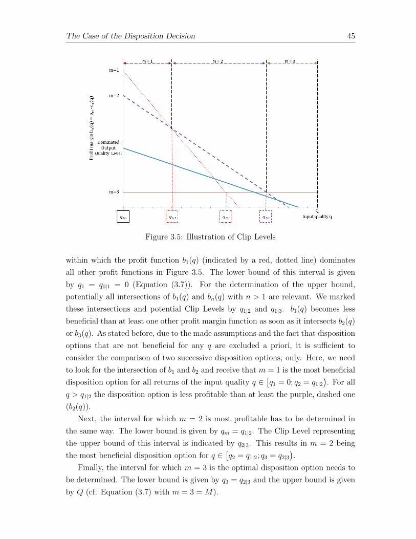
The Case of the Disposition Decision 45
Figure 3.5: Illustration of Clip Levels
within which the profit function b1(q) (indicated by a red, dotted line) dominates
all other profit functions in Figure 3.5. The lower bound of this interval is given
by q1 = q0|1 = 0 (Equation (3.7)). For the determination of the upper bound,
potentially all intersections of b1(q) and bn(q) with n > 1 are relevant. We marked
these intersections and potential Clip Levels by q1|2 and q1|3. b1(q) becomes less
beneficial than at least one other profit margin function as soon as it intersects b2(q)
or b3(q). As stated before, due to the made assumptions and the fact that disposition
options that are not beneficial for any q are excluded a priori, it is sufficient to
consider the comparison of two successive disposition options, only. Here, we need
to look for the intersection of b1 and b2 and receive that m = 1 is the most beneficial
disposition option for all returns of the input quality q ∈[q1 = 0; q2 = q1|2
). For all
q > q1|2 the disposition option is less profitable than at least the purple, dashed one
(b2(q)).
Next, the interval for which m = 2 is most profitable has to be determined in
the same way. The lower bound is given by qm = q1|2. The Clip Level representing
the upper bound of this interval is indicated by q2|3. This results in m = 2 being
the most beneficial disposition option for q ∈[q2 = q1|2; q3 = q2|3
).
Finally, the interval for which m = 3 is the optimal disposition option needs to
be determined. The lower bound is given by q3 = q2|3 and the upper bound is given
by Q (cf. Equation (3.7) with m = 3 = M).

The Case of the Disposition Decision 46
3.3.2 Decentralized Decision Makers - The Situation of the
Business Case
Next, we analyze the current business case setting. L commissions SP with all repro-
cessing activities. However, the ownership of the products that will be returned by
customers remains with L. SP receives end-of-lease returns from primary customers,
grades them and makes the disposition decision. After the required reprocessing
activities have been conducted by SP, the recovered units are sold via brokers to
the secondary market and recycled returns are sold on the raw materials market.
For these services, SP receives a service payment from L, whereas L as the product
owner receives the market prices achieved. The corresponding financial and material
flows are depicted in Figure 3.6.
(a) Material Flow (b) Financial Flow
Figure 3.6: Material and Financial Flow of the Business Case
According to Assumption 7, L acts as the Stackelberg leader. SP, the Stackel-
berg follower, has to decide on the disposition decision. As the Stackelberg leader, L
uses his knowledge of SP’s reaction to determine his service payment offering. Thus,
we first model SP’s decision on the disposition of returns and use the outcome to
analyze L’s choice of the amount of service payments.
SP’s Disposition Decision
According to Assumption 5, SP’s goal is to maximize his profit πBCSP . His profit

The Case of the Disposition Decision 47
function is given by the following equation:
πBCSP =
∫ Q
0
[sD(q) − cD(q)(q)] ∗ f(q) dq ∗X (3.10)
By comparing SP’s profit function with the central decision maker’s profit func-
tion (Equation (3.1)), we see that they differ only in terms of the payments that the
responsible decision maker receives: pD(q) for the central decision maker and sD(q)
here in our business case setting. This results in the same problem structure, and
we can therefore use the Clip Level formulation of Section 3.3.1, but we need to
change pm into sm.
Using these new Clip Levels, the intervals within which a certain output quality
level m is the most beneficial are now given by
m is optimal on[qBCm ; qBCm+1
)(3.11)
with
qBC1 = 0
qBCM+1 = Q
qBCm+1 = ∆c−1m+1(∆sm+1) ∀m = 1 . . . (M − 1)
(3.12)
with
∆sm+1 = sm − sm+1
and SP’s optimized profit function can be formulated accordingly:
πBCSP =M∑m=1
qBCm+1∫
qBCm
[sm − cm(q)] ∗ f(q) dq ∗X (3.13)
Note that this expression assumes that qBCm ≤ qBCm+1 ∀ m and thus that no dispo-
sition option is strictly dominated and thereby redundant. Whether this assumption
holds depends on the service payments sm. We address this issue when analyzing
the lessor’s decision problem below.
L’s Decision on Service Payments
L has to decide on the service payments that he offers to SP. These service payments
are output-quality-dependent (Assumption 3C). As a profit-maximizing actor, L’s

The Case of the Disposition Decision 48
aim is to maximize his profit function shown in Equation (3.14).
πBCL =
∫ Q
0
[pD(q) − sD(q)] ∗ f(q) dq ∗X (3.14)
Per unit reprocessed to output quality level m, L pays the service payment sm
and receives pm from the secondary or raw materials market. L’s profit depends on
SP’s disposition decision, which again depends on L’s choice of service payments.
Therefore, to maximize his profits, L needs to take into account SP’s reaction (i.e.
D(q)) when deciding on the service payments. L’s profit function can be expressed
in terms of the Clip Levels derived in Equation 3.12:
πBCL =M∑m=1
[pm − sm]
∆c−1m+1(∆sm+1)∫
∆c−1m (∆sm)
f(q) dq ∗X (3.15)
Recall from above that the expression for SP’s optimal decision is only valid for
∆c−1m (∆sm) ≤ ∆c−1
m+1(∆sm+1) ∀ m = 1 . . . (M − 1). (3.16)
We therefore impose this condition as a constraint for L’s choice of the service
payments. Note that we can do so without loss of generality since
∆c−1m (∆sm) > ∆c−1
m+1(∆sm+1) ∀ m = 1 . . . (M − 1)
implies that this option m is redundant. In this case we can increase sm such that
∆c−1m (∆sm) = ∆c−1
m+1(∆sm+1) ∀ m = 1 . . . (M − 1),
without affecting πBCL .
We observe from Equation (3.12) that SP’s disposition decision does not depend
on the absolute values of sm, but only on the difference between two successive
payments sm and sm+1. We therefore rewrite sm as
sm = sM +M−1∑m
∆sm+1 ∀m.
To ensure that SP has an incentive to become part of the reverse SC and conduct

The Case of the Disposition Decision 49
the reprocessing services, it is required that at least the recycling costs2 cM are offset
by the service payments received:
cM ≤ sM (3.17)
Using the aforementioned and cumulative distributions F (q) instead of integrals,
L’s profit function (Equation 3.15) can be rewritten:
πBCL =M∑m=1
[pm − sm]
∆c−1m+1(∆sm+1)∫
∆c−1m (∆sm)
f(q) dq ∗X
=
[− [p1 − s1] ∗ F (0)
+M−1∑m=1
[[pm − sm]− [pm+1 − sm+1]] ∗ F (∆c−1m+1(∆sm+1))
+ [pM − sM ] ∗ F (Q)
]∗X
=
[− [p1 − s1] ∗ F (0)
+M−1∑m=1
[∆pm+1 −∆sm+1] ∗ F (∆c−1m+1(∆sm+1))
+ [pM − sM ] ∗ F (Q)
]∗X
=
[M−1∑m=1
[∆pm+1 −∆sm+1] ∗ F (∆c−1m+1(∆sm+1))
+ [pM − sM ] ∗ F (Q)
]∗X
(3.18)
Note that the last transformation of Equation (3.18) is due to the continuous
distribution of input qualities which results in −[p1 − s1] ∗ F (0) = 0.
2Or any other lower bound that guarantees SP a sufficiently large margin to participate

The Case of the Disposition Decision 50
To summarize, we face a maximization problem subject to M inequality con-
straints:
πBCL =
[M−1∑m=1
[∆pm+1 −∆sm+1] ∗ F (∆c−1m+1(∆sm+1))
+ [pM − sM ] ∗ F (Q)
]∗X
(3.19)
subject to
∆c−1m (∆sm) ≤ ∆c−1
m+1(∆sm+1) ∀ m = 1 . . . (M − 1) (3.20)
cM ≤ sM (3.21)
We analyze this problem by considering the Karush-Kuhn-Tucker (KKT) condi-
tions. The necessary KKT condition for a (local) maximum is given in Table 3.4.
∂L∂sM≤ 0 sM ≥ 0 sM ∗ ∂L
∂sM= 0
∂L∂∆sm+1
≤ 0 ∆sm+1 ≥ 0 ∆sm+1 ∗ ∂L∂∆sm+1
= 0
∂L∂λM≥ 0 λM ≥ 0 λM ∗ ∂L
∂λM= 0
∂L∂λm≥ 0 λm ≥ 0 λm ∗ ∂L
∂λm= 0
Table 3.4: Karush-Kuhn-Tucker Condition for Local Maximum
We receive the following Lagrange equation (3.22) and KKT conditions (Equa-
tions (3.23) - (3.31)).
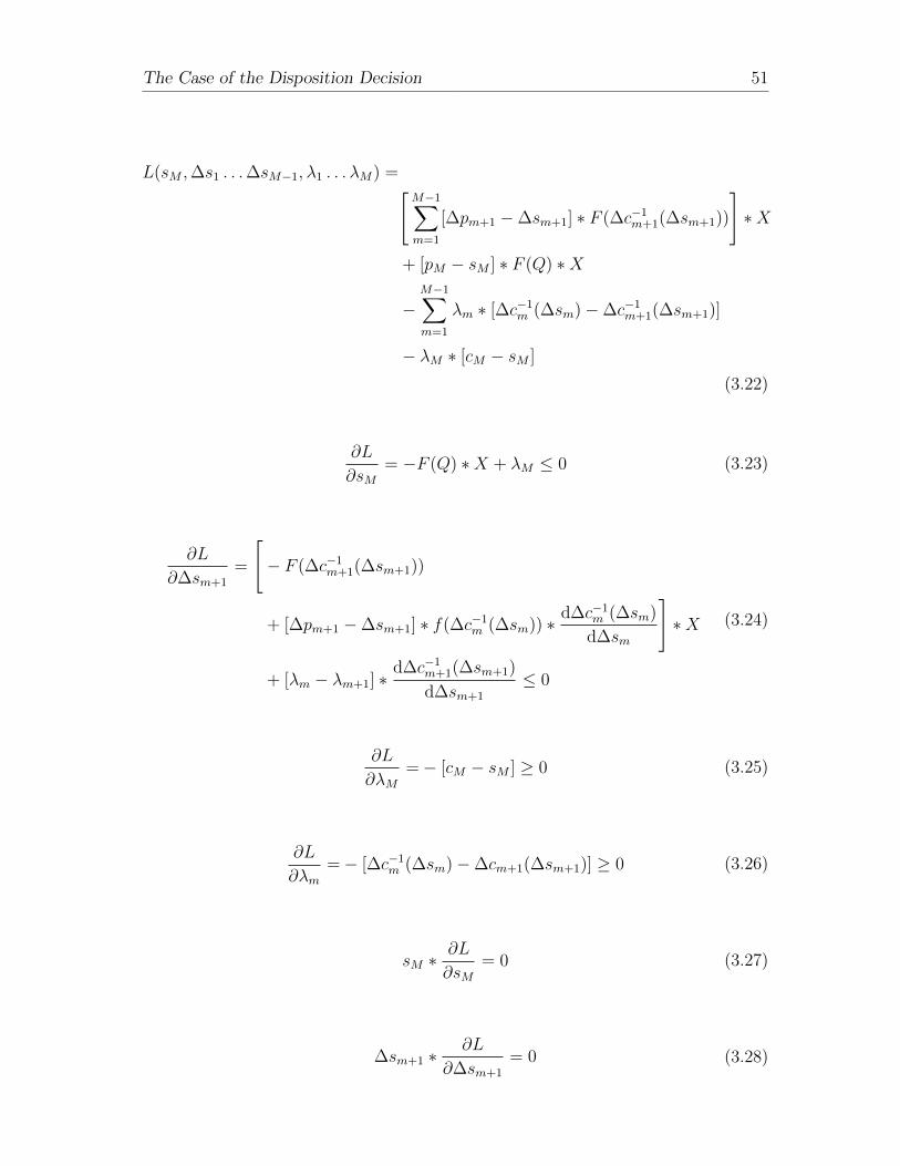
The Case of the Disposition Decision 51
L(sM ,∆s1 . . .∆sM−1, λ1 . . . λM) =[M−1∑m=1
[∆pm+1 −∆sm+1] ∗ F (∆c−1m+1(∆sm+1))
]∗X
+ [pM − sM ] ∗ F (Q) ∗X
−M−1∑m=1
λm ∗ [∆c−1m (∆sm)−∆c−1
m+1(∆sm+1)]
− λM ∗ [cM − sM ]
(3.22)
∂L
∂sM= −F (Q) ∗X + λM ≤ 0 (3.23)
∂L
∂∆sm+1
=
[− F (∆c−1
m+1(∆sm+1))
+ [∆pm+1 −∆sm+1] ∗ f(∆c−1m (∆sm)) ∗ d∆c−1
m (∆sm)
d∆sm
]∗X
+ [λm − λm+1] ∗d∆c−1
m+1(∆sm+1)
d∆sm+1
≤ 0
(3.24)
∂L
∂λM=− [cM − sM ] ≥ 0 (3.25)
∂L
∂λm=− [∆c−1
m (∆sm)−∆cm+1(∆sm+1)] ≥ 0 (3.26)
sM ∗∂L
∂sM= 0 (3.27)
∆sm+1 ∗∂L
∂∆sm+1
= 0 (3.28)
The Case of the Disposition Decision 52
λM ∗∂L
∂λM= 0 (3.29)
λm ∗∂L
∂λm= 0 (3.30)
sM ,∆s1 . . .∆sM−1, λ1 . . . λM ≥ 0 (3.31)
The goal of our further analysis is to check whether the decisions made in the
current business case setting are reverse SC optimal. Therefore, we compare the
profit function of a decentralized reverse SC (Equation (3.32)) and the reverse SC
profit function of a central decision maker (Equation (3.9)).
πBCRSC = πBCL + πBCSP
=M∑m=1
[pm − sm]
qBCm+1∫
qBCm
f(q) dq ∗X +M∑m=1
qBCm+1∫
qBCm
[sm − cm(q)] ∗ f(q) dq ∗X
=M∑m=1
qBCm+1∫
qBCm
[pm − cm(q)] ∗ f(q) dq ∗X
(3.32)
We see that profit functions πRSC and πBCRSC differ only in the borders of the
intervals, thus in the Clip Levels. In an integrated channel, all the input qualities
are reprocessed to the optimal output quality level m, meaning that each input
quality level is brought to that output quality level that achieves the highest margin
pm − cm(q). Considering the decentralized reverse SC’s profit, the margins are still
pm − cm(q), but the profit function differs with respect to the Clip Levels. In the
case of changed Clip Levels, not all input qualities are reprocessed to the reverse
SC optimal disposition option anymore. Hence, to gain a reverse SC optimal profit,
it is necessary to achieve the Clip Levels of our benchmark. qBCm+1 depends on the
chosen service payments sm (Equation 3.12), which makes a further analysis of these
service payments necessary.
Due to the structure of the service payments (and resulting from that profit func-
tion), it is possible to analyze the service payments sequentially. We first consider
L’s choice of sM .

The Case of the Disposition Decision 53
As L is a profit-maximizing actor, from Equation (3.23) it follows that λM > 0.
Hence, from Equation (3.29) we know that
∂L
∂λM
!= 0,
and we receive from Equation (3.25) that cM = sM . All subsequent payments sm
consist of this payment for recycling activities sM and the sum from m to (M − 1)
of ∆sm+1. The analysis of L’s choice of ∆sm+1 is separated into two parts. First,
we consider the case in which the lower bound = upper bound of an interval (i);
second, we turn to the case in which the lower bound < upper bound (ii).
In case (i), ∆c−1m (∆sm) = ∆c−1
m+1(∆sm+1). Thus, the interval is empty and a cer-
tain disposition option m is optimal for none of the input quality levels. Compared
with the integrated reverse SC, a previously optimal disposition option is no longer
achieved. Hence, without any further analysis, we know that the chosen service
payment cannot be reverse SC optimal.
In case (ii), ∆c−1m (∆sm) < ∆c−1
m+1(∆sm+1) ∀ m. Thus, all disposition options
m = 1 . . .M are optimal for some input quality levels q. In this case, ∂L∂λm
> 0
(Equation (3.26)) this results in λm!
= 0 (Equation (3.30)). Hence, Equation (3.24)
becomes
∂L
∂∆sm+1
=
[− F (∆c−1
m+1(∆sm+1))
+ [∆pm+1 −∆sm+1] ∗ f(∆c−1m (∆sm)) ∗ d∆c−1
m (∆sm)
d∆sm
]∗X ≤ 0
(3.33)
Without further knowledge of the properties of the density function, we are not
able to determine L’s optimal service payments explicitly. Nevertheless, it is possible
to show that L’s profit-optimizing choice of ∆sm+1 is not reverse SC optimal.
Comparing the two Clip Levels (Equation (3.7) and Equation (3.12)) one obtains
∆c−1m+1 (pm − pm+1)︸ ︷︷ ︸
:=∆pm+1
!= ∆c−1
m+1 (sm − sm+1)︸ ︷︷ ︸:=∆sm+1
(3.34)
which means that to achieve the central decision maker’s Clip Levels,
∆pm+1!
= ∆sm+1. (3.35)
If Equation (3.35) is fulfilled, Equation (3.33) < 0, thus from Equation (3.28) it

The Case of the Disposition Decision 54
follows that ∆sm+1!
= 0. No difference between two successive service payments
means that the lower and upper bounds of some intervals are equal to each other,
which - as argued before - is not reverse supply chain optimal.
To summarize, without knowledge of the probability distribution, it is not pos-
sible to specify the exact values of the service payments that L would choose to
optimize his profits. The specific solution depends on the shape of the probability
distribution function f(·) and needs to fulfill Equations (3.24), (3.28), and (3.31)
to maximize L’s profit function. However, a very interesting finding on the choice of
service payments needs to be emphasized. Even without any concrete information
on the probability distribution, we know that L’s choice is not reverse SC optimal.
Before we come to the discussion of this result, we make this analysis a little
more concrete. We analyze the decentralized SC for the specific case of linear cost
functions and uniformly distributed input qualities. These characteristics will be
used again in our numerical example in Section 3.4.
Consider the disposition options and corresponding profit margins bm with m =
1 . . . 3 introduced in the central setting. In Figure 3.7, we depict these disposi-
tion options, the corresponding profit margins, and the resulting Clip Levels qm+1.
Furthermore, we include the shift of profit margin functions and the resulting new
Clip Levels qBCm+1 in the case of decentralized decision making. While the reprocess-
ing costs are independent of the actor responsible for reprocessing activities, the
received payments vary from the centralized to the decentralized setting. Hence,
while the slope values cm of the profit margin functions remain, the intercept values
change from pm in the case of the central decision maker to sm in the case of de-
central decision making. This results in a parallel shift down of bm(q) by pm − sm.
In the example, L’s optimal choice of service payments sm is depicted. The profit
margin functions bBCm (q) relevant to SP’s choice of the Clip Levels qBCm+1 are given by
bBCm (q) = sm − cm ∗ q.To determine L’s choice of service payments, his profits need to be taken into
consideration. L’s profit resulting from SP’s disposition decision is shown as the
shaded areas in Figure 3.8. The shaded areas result from the following consideration:
per unit of a returned product of input quality q reprocessed to m, L receives pm
and has to pay sm. Thus, in the case of m = 1, L’s profit results from
(p1 − s1) ∗ (qBC2 − qBC1 )︸ ︷︷ ︸Interval of input qualities that is reprocessed to m=1
.

The Case of the Disposition Decision 55
Figure 3.7: Change of Profit Margins and Clip Levels Compared to the IntegratedSetting, Given Linear Costs and Uniformly Distributed Input Qualities
Figure 3.8: Resulting Profit of L, Given Linear Costs and Uniformly DistributedInput Qualities

The Case of the Disposition Decision 56
As a profit-maximizing actor, his objective is to maximize these areas by optimizing
his profit function:
πBCL =
[M−1∑m=1
[pm − sm] ∗ F
([sm − sm+1
cm − cm+1︸ ︷︷ ︸:=qBC
m+1
− sm−1 − smcm−1 − cm︸ ︷︷ ︸
:=qBCm
])
+ [pM − sM ] ∗ F
([Q− sM−1 − sM
cM−1 − cM︸ ︷︷ ︸:=qBC
M
])]∗X
=
[M−1∑m=1
[∆pm+1 −∆sm+1] ∗ F
(∆sm+1
∆cm+1
)
+ [pM − sM ] ∗ F (Q)
]∗X
(3.36)
subject to
∆sm∆cm
≤ ∆sm+1
∆cm+1
∀ m = 1 . . . (M − 1) (3.37)
cM ≤ sM (3.38)
Clip Levels are determined by comparing two successive profit margins bBCm and
bBCm+1:
sm − cm ∗ q!
= sm+1 − cm+1 ∗ q
qBCm+1 =∆sm+1
∆cm+1
Under the assumption of a concave objective function and linear constraints,
KKT is sufficient to determine L’s optimal choice of service payments.

The Case of the Disposition Decision 57
L(sM ,∆s1 . . .∆sM−1, λ1 . . . λM) =
[M−1∑m=1
[∆pm+1 −∆sm+1] ∗ F
(∆sm+1
∆cm+1
)]∗X
+ [pM − sM ] ∗ F (Q) ∗X
−M−1∑m=1
λm
[∆sm∆cm
− ∆sm+1
∆cm+1
]− λM ∗ [cM − sM ]
(3.39)
∂L
∂sM= −F (Q) ∗X + λM ≤ 0 (3.40)
∂L
∂∆sm+1
= [∆pm+1 − 2 ∗∆sm+1] ∗ 1
∆cm+1
∗ 1
Q∗X
+ [λm − λm+1] ∗ 1
∆cm+1
≤ 0
(3.41)
∂L
∂λM= −[cM − sM ] ≥ 0 (3.42)
∂L
∂λm= −
[∆sm∆cm
− ∆sm+1
∆cm+1
]≥ 0 (3.43)
sM ∗∂L
∂sM= 0 (3.44)
∆sm+1 ∗∂L
∂∆sm+1
= 0 (3.45)
λM ∗∂L
∂λM= 0 (3.46)

The Case of the Disposition Decision 58
λm ∗∂L
∂λm= 0 (3.47)
sM ,∆s1 . . .∆sM−1, λ1 . . . λM ≥ 0 (3.48)
Analogous to the general analysis we derive from Equations (3.40), (3.42), and
(3.46) that sM!
= cM . Analogous to case (ii) above, only if
∆sm∆cm
<∆sm+1
∆cm+1
(3.49)
it is assured that all not redundant output quality levels of a centralized case are
achieved. Thus Equation (3.43) > 0, which requires λm!
= 0 to fulfill Equation (3.47).
Hence Equation (3.41) becomes
∂L
∂∆sm+1
= [∆pm+1 − 2 ∗∆sm+1] ∗ 1
∆cm+1
∗ 1
Q∗X ≤ 0. (3.50)
Furthermore, as upper and lower bounds are not identical, it is given that
∆sm+1 > 0. Hence to fulfill Equation (3.45), Equation (3.50)!
= 0. Finally, we
receive from Equation (3.50) the following result for L’s choice of service payments:
∆sm+1 =∆pm+1
2(3.51)
Since in Equation (3.51) ∆sm+1 6= ∆pm+1 the service payments received under
the assumption of linear costs and uniformly distributed input qualities q, are not
equal to the reverse SC optimal choice of service payments.
Because L will not transfer ∆pm+1 completely, but ∆sm+1 = ∆pm+1
2, Clip Levels
of a decentralized decision maker (∆sm+1
∆cm+1) will be smaller than those of a central
decision maker (∆pm+1
∆cm+1). Compared with the integrated case, this results in smaller
intervals within which an output quality level m is most beneficial. This holds for
all intervals except for the “last” one, that is, the interval within which the input
qualities are brought to the worst achieved output quality level. For this interval,
two possibilities need to be distinguished: either it becomes larger or it becomes
smaller as well and - compared with the integrated SC - higher, that is, worse
output quality levels are achieved. Hence, compared with the integrated reverse
SC, fewer input quality levels are reprocessed to the output option achieving higher
market prices and more input quality levels are reprocessed to a worse output quality

The Case of the Disposition Decision 59
level, achieving lower market prices. Hence, depending on the actual batch structure
(with respect to quality), the reverse SC profit is affected.
Besides this negative impact on the reverse SC profit, there is a further important
aspect to mention. Smaller Clip Levels will result in the fact that returned products
of a certain input quality possibly are reprocessed to suboptimal output quality
levels. Accordingly, some input quality levels that are in fact reusable may be
recycled - thus, the inherent value is wasted. This factor is optimal neither with
respect to profit considerations nor with regard to environmental objectives. For all
the disposition options in between, the change in the interval size depends on the
characteristics of the situation considered.
In the following, we return to the general case. Without knowledge of the proba-
bility distribution of the input qualities, we cannot state L’s actual choice of service
payments. However, due to L’s preference to choose ∆sm+1 6= ∆pm+1, we know
that Clip Levels will not be optimal. We know that ∆sm+1 < ∆pm+1, resulting in
Clip Levels that are smaller than those of a central decision maker. In contrast to
the above special case, we cannot tell exactly how much smaller the Clip Levels are
compared with the integrated SC. However, it is still possible to make statements
on the effects on two of the intervals within which a certain disposition option m is
optimal:
1. The interval within which m = 1 is the most beneficial option becomes smaller
than in the integrated reverse SC, that is, compared with the central decision
maker, fewer input quality levels are reprocessed to m = 1.
2. Either the interval of the worst achieved output quality level becomes larger
than in the integrated reverse SC or worse disposition option becomes optimal
for some input quality levels.
The rationale behind this SC deficiency is that the achievable margin of pm −cm(q) is shared between the two actors involved:
pm − sm︸ ︷︷ ︸L
+ sm − cm(q)︸ ︷︷ ︸SP
. (3.52)
While a central decision maker receives market prices pm, in a decentralized
reverse SC, SP as the reprocessing actor receives sm from L. L’s optimal choice of
service payments sm < pm results in a lower incentive of the reprocessing actor,
SP, to incur higher reprocessing costs cm(q). Hence, compared with the integrated
reverse SC, only better input qualities q (which incur lower costs) are reprocessed
to m.

The Case of the Disposition Decision 60
3.3.3 Decentralized Decision Makers - The Service Provider
Acquires Product Returns
To overcome the reverse SC deficiency identified in the analysis of our business
case, we consider an alternative contract structure and show that it coordinates
the setting. The aim is to gain reverse SC optimal profits by achieving reverse SC
optimal Clip Levels. In Chapter 2, we provided an overview of the mechanisms
coordinating diverse forward SC settings. Some of these mechanisms have been
transferred successfully to a reverse SC setting. Based on our discussions with
ARC, we investigate the idea that the reprocessing company not only executes the
reprocessing activities but also assumes ownership of the returned products.
In this section, L sells all of his end-of-lease products to SP3 and receives a certain
acquisition price per unit. It is assumed that the same acquisition price is paid for
each return regardless of the future disposition decision. SP becomes the new owner
of the returned products, makes the disposition decision, and conducts the required
reprocessing activities. As the owner of the reprocessed products, SP receives the
achievable market prices and has to pay for the reprocessing costs as well as the
acquisition price. The corresponding financial flows are depicted in Figure 3.9. The
material flow remains as in the current business case setting (Figure 3.6).
In this setting, again two independent actors have to make a decision that influ-
ences the reverse SC’s profit. First, L decides on the acquisition price and second,
SP makes the disposition decision. This disposition decision is influenced by sev-
eral factors. As in the previous settings, the actual input quality of the returned
products and the resulting reprocessing costs are of relevance. Now, though, the SP
receives the market prices on the one hand and additionally has to take into account
acquisition price on the other hand. As SP’s profit is affected by the acquisition
price, L needs to consider the effects of his choice of the acquisition price in his
decision making.
SP’s Disposition Decision
In this setting, SP receives the market prices pm. Besides the reprocessing cost
cm(q), he has to pay the acquisition price pac per unit. pac is determined by L.
As L cannot control for the input qualities, pac is not determined for each input
quality individually but is based on an expected distribution of input qualities and
further considerations that we address below. Thus, unsorted batches are sold for a
3Although SP no longer acts as the service provider, we retain the naming of the actors of theprevious sections.
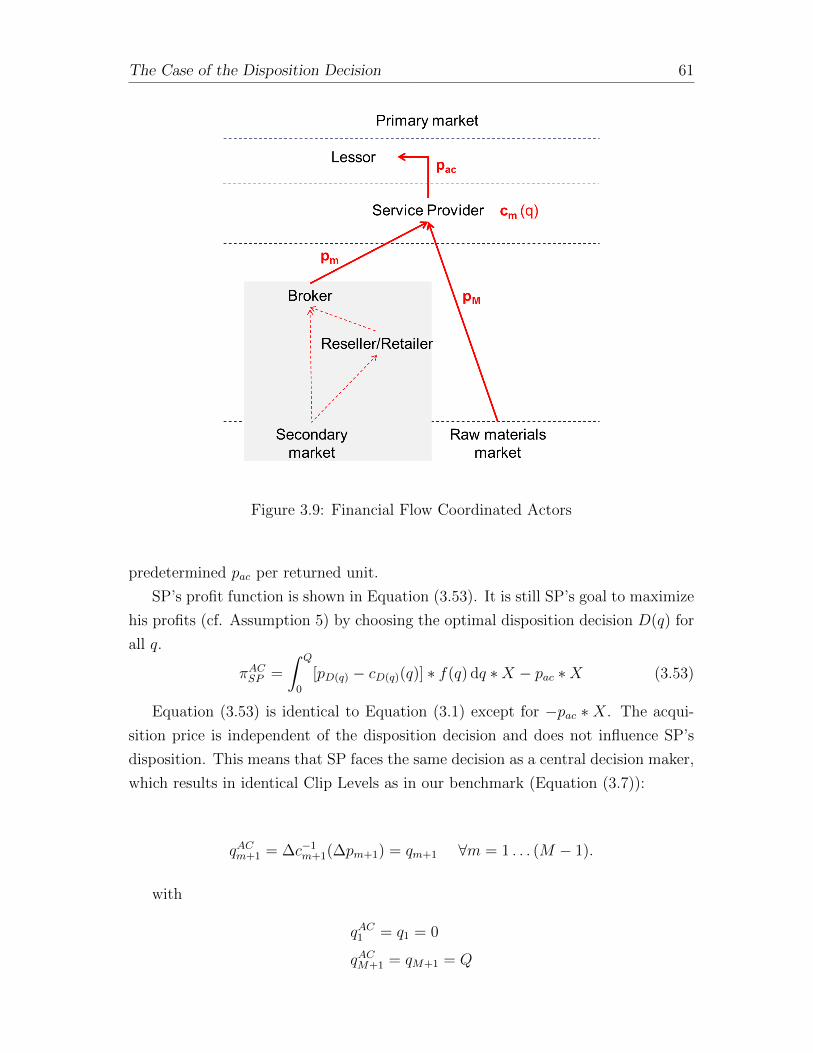
The Case of the Disposition Decision 61
Figure 3.9: Financial Flow Coordinated Actors
predetermined pac per returned unit.
SP’s profit function is shown in Equation (3.53). It is still SP’s goal to maximize
his profits (cf. Assumption 5) by choosing the optimal disposition decision D(q) for
all q.
πACSP =
∫ Q
0
[pD(q) − cD(q)(q)] ∗ f(q) dq ∗X − pac ∗X (3.53)
Equation (3.53) is identical to Equation (3.1) except for −pac ∗ X. The acqui-
sition price is independent of the disposition decision and does not influence SP’s
disposition. This means that SP faces the same decision as a central decision maker,
which results in identical Clip Levels as in our benchmark (Equation (3.7)):
qACm+1 = ∆c−1m+1(∆pm+1) = qm+1 ∀m = 1 . . . (M − 1).
with
qAC1 = q1 = 0
qACM+1 = qM+1 = Q

The Case of the Disposition Decision 62
Figure 3.10: Comparison of Clip Levels in the Benchmark and in Case of Acquisitionof Returned Products
Achieving the same Clip Levels means that under this contract type the same
disposition decision as in the centralized case is made. Hence, all the returned
products are reprocessed to the reverse SC optimal output quality level.
Using the simplified example of linear cost functions and uniformly distributed
input qualities, Figure 3.10 shows the Clip Levels in the case that the SP acquires
the returned products compared with our benchmark.
Having SP acquire the returns coordinates the disposition decision and results
in reverse SC optimal profits. Compared with the current business case setting, in
the coordinated case additional profits are gained in the CLSC. The question than
arises of how to share these additional benefits between L and SP, that is, how to
determine pac.
L’s Decision on the Acquisition Price
L offers returned end-of-lease units and decides on pac. This predetermined acquisi-
tion price pac per unit sold to SP is the only payment that L has to consider. Hence,

The Case of the Disposition Decision 63
his profit function is given by
πACL = pac ∗X (3.54)
L’s profit no longer depends on the disposition decision but only on the choice of
pac. To achieve his goal of profit maximization, L wants to maximize pac. However,
L has to consider SP’s reaction. As pac has a negative impact on SP’s profit, L has
to take into account whether SP has an incentive - by means of profit - to participate
in the contract or not. Based on the participation constraints of both actors, upper
and lower bounds for pac can be stated.
From L’s profit function, we can derive a lower bound of the acquisition price.
If L’s profit is lower than his current (business case) profit, L has no incentive to
change the setting. Hence, a lower bound can be stated (Equation (3.55)).
πACL ≥ πBCL
pac ∗X!
≥ πBCL
pac ≥πBCLX
(3.55)
An upper bound of pac can be stated from the argument that SP’s profit needs
to be positive (Equation (3.57)).
πACSP =M∑m=1
qm+1∫qm
[pm − cm(q)] ∗ f(q) dq ∗X
︸ ︷︷ ︸:=πC
RSC
−pac ∗X(3.56)
πACSP!> 0
pac <πCRSCX
(3.57)
Alternatively, one can argue that SP, as well, takes part only if πACSP ≥ πBCSP . This
results in a tighter upper bound:
πCRSC − pac ∗X ≥ πBCSP

The Case of the Disposition Decision 64
pac ≤πCRSC − πBCSP
X. (3.58)
We show that this rather simple strategy results in the same disposition deci-
sions as in the case of a central decision maker: all the returns are reprocessed to
the optimal output quality level from a reverse SC perspective. Consequently, the
reverse SC profit equals the optimal reverse SC profit achieved by a central decision
maker. The resulting reverse SC profit is split between L and SP depending on the
acquisition price. Thereby, the negotiations between SP and L on pac take place
within the upper and lower bounds introduced above.4
Summarizing, this contract does not only coordinate the decentralized reverse
SC, but furthermore it is a very flexible solution. While the aforementioned bounds
are based on pure profit considerations, the negotiation process itself may be influ-
enced by market power and certain risks. One major risk that needs to be considered
is the risk of uncertainty with regard to the actual input quality of the returned prod-
ucts. Above, we assume quality-independent acquisition prices. This assumption is
realistic in our case, as we observed long-term contracts between L and SP. In such
settings, this assumption is justified as the actual realization of the distribution of
input qualities within one batch may differ from the expected one, nevertheless, in
the long run, the deviations should be balanced.
However, a disposition independent pac bears some risk that needs to be consid-
ered in the case of interactions that take place only once. In such settings, it can be
expected that SP would renegotiate pac if the grading shows that the input qualities
within a batch are worse than announced. The possibility to renegotiate shifts the
risk to L, as the risk of the actual quality means for L that the determined pac might
be too low for certain batch structures, but on the other hand L needs to lower pac
in the case of lower qualities than announced. In such a setting, it may be assumed
that L has the incentive to choose an unreasonably high price at the beginning as
L knows that SP will claim a lower price for returns of low quality.
Taking one step further, such a renegotiation mechanism could also be introduced
by L to renegotiate with his primary customers in the case that the input quality
does not match the agreed return quality level. As we regard the interplay between
SP and L, this consideration is beyond our recent focus. However, it is certainly an
interesting idea for further research (cf. Chapter 3.5).
Besides SP’s profit-driven considerations regarding whether to take part or not,
for the implementation of the suggested contract it is also of interest whether L
4The range of the acquisition price negotiation is illustrated in the numerical example (Sec-tion 3.4, Figure 3.13).

The Case of the Disposition Decision 65
is interested in selling its end-of-lease returns to a reprocessing company at all.
Until now, we have considered lessors in general. When it comes to selling the
returned IT hardware, the kind of company that is acting as lessor probably becomes
relevant. Potentially, two kinds of companies need to be distinguished here: OEMs
and financial service providers. In the case of an OEM, protection of the brand image
is a relevant aspect (Ferguson, 2010). Many OEMs are afraid of losing control of
the reprocessing activities of products that are labeled with their brand. Thus, the
consideration of potential damage to the brand image needs to be taken into account
here as well. This aspect is not relevant in the case that a financial service provider
acts as the lessor.
3.4 Numerical Example
In the following, we illustrate our analysis on the basis of a short example. First,
the data used in this example are presented; then the decisions made in the afore-
mentioned settings are shown.
A batch consisting of X = 100 end-of lease units of an IBM notebook (Intel Core
2 Duo, 1.6 Ghz, and 14” screen) is considered in the following. These notebooks
can be of different, continuous input qualities q ∈ [0;Q]. Input quality q = 0
represents product returns in an “as new” condition. The other end of the input
quality spectrum is given by Q. Returns of input quality Q require severe repair
and have cosmetic issues. To allow for a variety of input qualities, we chose to scale
Q = 5.
In this example, m = 5 different output quality levels can be achieved. The
worst output quality level M = 5 is the recycling option. All the other options
represent recovery of the returned product. The possibility to upgrade a returned
unit to achieve higher market values is included in our example. We consider two
different components that can be upgraded: the random-access memory (RAM) and
the hard disk drive (HDD). The current version of returned notebooks includes a
HDD of 100 GB and a 2 GB RAM. Without any upgrading, output quality level
m = 4 can be achieved. Thus, depending on the input quality level, repair, cosmetic
rework, and exchange of defective parts need to be conducted. Better output quality
levels m < 4 are achieved by updating one of the two mentioned components or both
of them. An upgrade to a 200 GB hard disk (m = 3) is possible as well as additional
RAM of 2 GB (m = 2). The best standard (m = 1) is achieved in the case that
both components are updated.
The achievable market prices attached to certain product configurations are

The Case of the Disposition Decision 66
m RAM Hard disk Price1 4 GB 200 GB HDD 188 e2 4 GB 100 GB HDD 177 e3 2 GB 200 GB HDD 163 e4 2 GB 100 GB HDD 152 e5 Recycling 5 e
Table 3.5: Prices on Raw Materials Market and Secondary Market
taken from the so-called BFL IT Index.5 The index is provided by BFL Leas-
ing, which is part of Volksbanken Raiffeisenbanken Leasing Group. BFL Leasing
refers to itself as an IT specialist that can look back on more than thirty years of
experience in IT financing. This index is also used by ARC to forecast prices on
secondary markets. The achievable market prices depend on the technological stan-
dard of the components included. These output-quality-dependent prices are shown
in Table 3.5. The price achievable on the raw materials market is assumed to be
e 5 per notebook.6
An underlying aspect of the disposition decision is the cost cm(q) of reprocessing
a unit of input quality q to output quality m. Neither the BFL IT Index nor ARC
provides any information concerning reprocessing costs. Therefore, we need to refer
to literature evidence at this point. In a study on trade-in rebates for IT equipment,
Agrawal et al. (2008) provide information on remanufacturing costs as a fraction of
manufacturing costs. As we are studying the same industry, we assume this ratio
to be appropriate for the following example.
To achieve an output quality level m, input-quality-dependent and linear repro-
cessing costs cm(q) occur, with cm(q) = cost ratiom(q) ∗manufacturing cost. In our
example, manufacturing costs of e 375 are assumed. According to Agrawal et al.
(2008), for IT hardware, the cost ratio is between 0.04 and 0.20. There is no clear
statement in the paper, but as no upgrading is mentioned, it may be assumed that
this ratio is valid for reprocessing to a standard technological level, which corre-
sponds to m = 4 in our example. Besides the output quality level m, the input
quality q of returned products is a driver of the reprocessing costs. To have the
possibility to be within the suggested ratio range, we determine the cost ratio to
reprocess one return of input quality level q to m = 4 to be 0.04. Hence, depending
on the input quality q ∈ [0; 5], we receive cost ratios ∈ [0.04; 0.2].
5http://www.bfl-it-index.de6According to WDR / SWR / BR-alpha (2013), one ton of notebooks contains precious metals
that are worth about e 1700. Assuming a weight of 2.5 kilos per laptop,1700Euro
t
1000 kgt
∗ 2.5 kgnotebook ≈
5 Euronotebook are considered here as achievable price on the raw materials market.
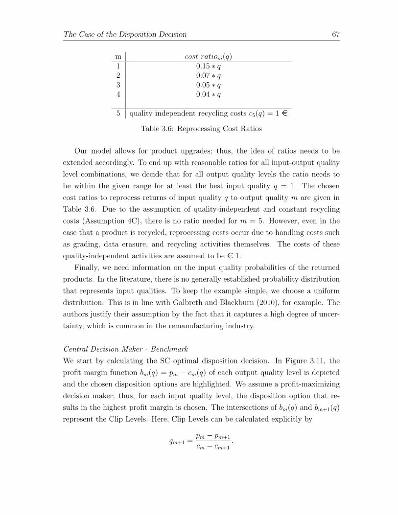
The Case of the Disposition Decision 67
m cost ratiom(q)1 0.15 ∗ q2 0.07 ∗ q3 0.05 ∗ q4 0.04 ∗ q
5 quality independent recycling costs c5(q) = 1 e
Table 3.6: Reprocessing Cost Ratios
Our model allows for product upgrades; thus, the idea of ratios needs to be
extended accordingly. To end up with reasonable ratios for all input-output quality
level combinations, we decide that for all output quality levels the ratio needs to
be within the given range for at least the best input quality q = 1. The chosen
cost ratios to reprocess returns of input quality q to output quality m are given in
Table 3.6. Due to the assumption of quality-independent and constant recycling
costs (Assumption 4C), there is no ratio needed for m = 5. However, even in the
case that a product is recycled, reprocessing costs occur due to handling costs such
as grading, data erasure, and recycling activities themselves. The costs of these
quality-independent activities are assumed to be e 1.
Finally, we need information on the input quality probabilities of the returned
products. In the literature, there is no generally established probability distribution
that represents input qualities. To keep the example simple, we choose a uniform
distribution. This is in line with Galbreth and Blackburn (2010), for example. The
authors justify their assumption by the fact that it captures a high degree of uncer-
tainty, which is common in the remanufacturing industry.
Central Decision Maker - Benchmark
We start by calculating the SC optimal disposition decision. In Figure 3.11, the
profit margin function bm(q) = pm − cm(q) of each output quality level is depicted
and the chosen disposition options are highlighted. We assume a profit-maximizing
decision maker; thus, for each input quality level, the disposition option that re-
sults in the highest profit margin is chosen. The intersections of bm(q) and bm+1(q)
represent the Clip Levels. Here, Clip Levels can be calculated explicitly by
qm+1 =pm − pm+1
cm − cm+1
.

The Case of the Disposition Decision 68
Figure 3.11: Profit Margins and Disposition Decision of a Central Decision Maker
Given the data introduced, the following disposition decisions are made in the
case of a central decision maker:
q D(q)q ∈ [0.00; 0.37) m = 1q ∈ [0.37; 1.87) m = 2q ∈ [1.87; 2.93) m = 3q ∈ [2.93; 5.00) m = 4
Table 3.7: Disposition Decision of a Central Decision Maker
This results in a profit of e 14,928 for a centralized reverse SC in our example.7
Decentralized Decision Makers - The Situation of the Business Case
We compare the outcome of the decentralized strategy observed in the business case
with the above centralized decisions and resulting reverse SC profit. L’s profit de-
pends on SP’s disposition decision, which depends on L’s choice of service payments.
Hence, anticipating SP’s disposition decision, L determines the service payments.
Due to an assumed uniform distribution function of input quality levels, we are
able to determine the optimal values for the service payments according to Equa-
7Remark: In this example, the recycling option (m = 5) is chosen for none of the input qualityclasses. However, cases like breakdowns of particularly expensive components, like the mother-board, are not covered by the exemplary cost structure.

The Case of the Disposition Decision 69
s1 92.50s2 87.00s3 80.00s4 74.50s5 1.00
Table 3.8: L’s Optimal Decision on Service Payments [in e]
tion (3.51). Analogous to the considerations in Chapter 3.3.2, the service payments
for recycling are fixed as equal to the recycling cost. L’s profit-optimizing choice of
service payments is given in Table 3.8.
Based on these service payments and the grading outcome, SP makes the dis-
position decision. SP’s profit margin functions bBCm (q) are depicted in Figure 3.12.
Again, the profit-optimizing actor SP chooses for each input quality level the dis-
position option that results in the highest profit margin. The chosen disposition
options are highlighted in Figure 3.12. Again, the intersection of successive profit
margin functions need to be determined and Clip Levels are given by
qBCm+1 =sm − sm+1
cm − cm+1
.
Given the data introduced, a decentralized decision maker makes the following
disposition decision:
q D(q)q ∈ [0.00; 0.18) m = 1q ∈ [0.18; 0.93) m = 2q ∈ [0.93; 1.47) m = 3q ∈ [1.47; 5.00) m = 4
Table 3.9: Disposition Decision of a Decentral Decision Maker
By comparing the chosen disposition options of the integrated and the decen-
tralized reverse SC, it can easily be seen that they differ from each other. In both
settings, the returned products are reprocessed to output quality levels m = 1 . . . 4
and none of the input quality levels q ∈ [0; 5] is reprocessed to m = M . However,
the disposition decisions differ with respect to the Clip Levels and thus which input
quality levels are reprocessed to which disposition option. The profits that result
from the decentralized decision maker’s disposition decision are shown in Table 3.10.
Taking the sum of both actors’ profit, we receive a reverse SC profit of e 13,732.
Thus, the reverse SC profit in the current decentralized setting is below the profit
that is achieved in the centralized setting. The uncoordinated strategy results in a

The Case of the Disposition Decision 70
Figure 3.12: Profit Margins for SP and Disposition Decision of a Decentral DecisionMaker
Lessor: 8062 eService Provider: 5670 eReverse Supply Chain: 13,732 e
Table 3.10: Profits Business Case
reverse SC profit decrease of 8% for the example data.
Decentralized Decision Makers - The Service Provider Acquires Product Returns
Making SP acquire all the returned products for a certain price pac was shown to co-
ordinate the introduced problem setting. According to this strategy, the disposition
decisions of a decentralized decision maker are made as they are made by a central-
ized decision maker. Therefore, the resulting reverse SC profit is equal to that of the
integrated reverse SC. The remaining question is how this (additional) reverse SC
profit is split between the two actors. As already explained in the analysis section,
different factors influence the determination of this acquisition price. Regardless
of the knowledge of the strength of different factors, we can state a lower and two
potential upper bounds of pac. According to these boundaries (Equations (3.55)
and (3.58), or (3.57)), in our example, the negotiation of the acquisition price takes
place in the range of e 80.62 to e 92.58 (e 149.28). In Figure 3.13, different actors’
profits are depicted depending on the various possible acquisition prices.

The Case of the Disposition Decision 71
Figure 3.13: Split of (Additional) Reverse Supply Chain Profit Depending on theAcquisition Price
3.5 Discussion
We introduced the ARC business case (Section 1.3) and highlighted the need to
coordinate the disposition decision (Section 1.4). The focus of our analysis is on two
actors, L and SP. As argued before, this is a reasonable limitation due to the leasing
context and long-term agreements with brokers. Furthermore, due to the ongoing
trend in the IT hardware industry to outsource production and focus on research
and development, the involvement of service providers as reprocessing actors can be
expected to be of increasing interest.
The decisions in the decentralized setting observed in the business case are shown
to be not reverse SC optimal (Section 3.3.2). To overcome this SC deficiency, we
introduced an alternative strategy in Section 3.3.3. The strategy suggests that
the current material flows remain, but the financial flows are changed, due to the
acquisition of product returns by SP. It was shown that reverse SC optimal profits
are achievable by this strategy. We found upper and lower bounds of the range
within which the negotiation on the acquisition price takes place. Furthermore, we
highlighted the considerations that influence this negotiation process.
Our analysis provides helpful results for the reverse SC setting considered and
provides an easy-to-implement strategy that coordinates the disposition decision in a
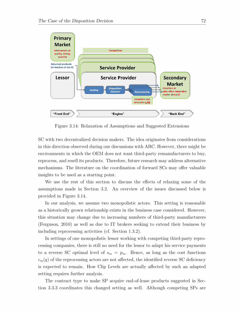
The Case of the Disposition Decision 72
Figure 3.14: Relaxation of Assumptions and Suggested Extensions
SC with two decentralized decision makers. The idea originates from considerations
in this direction observed during our discussions with ARC. However, there might be
environments in which the OEM does not want third-party remanufacturers to buy,
reprocess, and resell its products. Therefore, future research may address alternative
mechanisms. The literature on the coordination of forward SCs may offer valuable
insights to be used as a starting point.
We use the rest of this section to discuss the effects of relaxing some of the
assumptions made in Section 3.2. An overview of the issues discussed below is
provided in Figure 3.14.
In our analysis, we assume two monopolistic actors. This setting is reasonable
as a historically grown relationship exists in the business case considered. However,
this situation may change due to increasing numbers of third-party manufacturers
(Ferguson, 2010) as well as due to IT brokers seeking to extend their business by
including reprocessing activities (cf. Section 1.3.2).
In settings of one monopolistic lessor working with competing third-party repro-
cessing companies, there is still no need for the lessor to adapt his service payments
to a reverse SC optimal level of sm = pm. Hence, as long as the cost functions
cm(q) of the reprocessing actors are not affected, the identified reverse SC deficiency
is expected to remain. How Clip Levels are actually affected by such an adapted
setting requires further analysis.
The contract type to make SP acquire end-of-lease products suggested in Sec-
tion 3.3.3 coordinates this changed setting as well. Although competing SPs are
The Case of the Disposition Decision 73
considered, each SP makes the reverse SC optimal disposition decision, as the fi-
nancial flows between L and SP remain. However, in the case of our proposed co-
ordinating strategy, the competition between SPs possibly strengthens L’s position.
Using his stronger position, L can take advantage of the negotiation range of acqui-
sition prices, thus shifting the additional benefits, which result from a coordinated
disposition decision, to L.
Analogous to the standard SCM literature, we made the assumption that both
actors have knowledge of SP’s reprocessing cost structure (Assumption 4D). In our
analysis, we indicated that L’s decision on service payments relies on the knowledge
of SP’s corresponding Clip Level, namely the disposition decision. Hence, without
knowledge of SP’s cost structure, an additional level of uncertainty with regard to
SP’s disposition decision occurs.
Lack of knowledge of SP’s cost structure is not expected to make L transfer
∆pm+1 to SP completely. Hence, the situation in which SP chooses reverse SC
sub-optimal Clip Levels remains. This brings us to the question of whether the
relaxation of Assumption 4D affects the coordinating strategy. L’s profit does not
depend on the disposition of returns. This means that the lack of knowledge of SP’s
disposition decision is not damaging and the strategy still coordinates the setting.
However, to determine the acquisition price, among others, SP’s resulting profit is of
relevance to find the upper bounds of pac. Hence, the negotiation process concerning
pac may be affected by the relaxation.
Currently, long-term agreements with brokers exist. Relaxing the resulting as-
sumption of given, known, and unrestricted market demand incorporates the “back
end” into our analysis. We propose several research ideas in this direction.
If the assumption of unlimited market demand is relaxed, market saturation of
the total market or some brokers’ networks is an aspect that needs to be taken into
account in the analysis. As a consequence, the market prices are valid for certain
amounts reprocessed to a given output quality level only. Then, the disposition deci-
sion depends not only on the input quality of returns but also on the market demand
for certain output quality levels and previously sold amounts. Market saturation po-
tentially affects the disposition decision in all the settings considered. Thus, to be
able to make reliable conclusions, further analysis is required.
If the market demand is no longer given and known, the factors influencing the
demand of reprocessed products represent a further potential research focus. In
the traditional SCM literature, besides prices, sales effort represents one of these
factors. How does sales-effort-dependent demand affect our reverse SC setting? The
business case’s decentralized decision maker, SP, receives service payments from L

The Case of the Disposition Decision 74
and incurs reprocessing costs. In the case of sales-effort-dependent demand, SP
additionally incurs costs for sales effort. He does not directly benefit from this
effort, as L receives the market prices per unit sold to the secondary market. Hence,
besides the disposition decision, an additional coordination obstacle with regard to
the level of sales effort arises.
According to Cachon (2003), coordination of the sales-effort problem can be
achieved by simply sharing the costs of the sales effort if
1. the supplier can observe the retailer’s exerted effort,
2. the retailer’s effort is verifiable to the courts, and
3. the supplier directly benefits from the exerted effort.
Thus, it needs to be determined whether the above criteria are fulfilled. If they
are not fulfilled, besides the sub-optimal Clip-Levels, an additional coordination
requirement exists with respect to the choice of the sales effort: a setting that
provides potential for further research projects. However, even though the above
criteria are potentially fulfilled and reverse SC optimal sales effort is achieved, we still
face the problem of SP’s sub-optimal choice of Clip Levels as the service payments
for reprocessing activities are unchanged.
Does the suggested strategy to make the SP acquire the returned products co-
ordinate the extended setting as well? To be considered here is that it is no longer
given that all the reprocessed units can be sold. This probably results in the case
that SP no longer acquires all the returned units, which affects L’s profits. Hence,
L benefits from increased sales efforts resulting in higher demands. Given that the
above criteria hold, the sales effort costs can be split between the actors involved
and SP exerts the reverse SC optimal sales effort. What about SP’s Clip Level
decision under this strategy? Does the suggested strategy still result in the reverse
SC optimal disposition decision or does the sales-effort-dependent demand affect
SP’s decision? This depends on the characteristics of the sales effort costs. In the
case that these costs are independent from the output quality level, SP’s disposition
decision is still reverse SC optimal. Otherwise, further analysis is required.
The incorporation of the “front end” provides further alternatives to extend our
analysis. Uncertainty with respect to timing, quantity, and quality is commonly
mentioned as a complicating characteristic of reverse SC. Due the assumption of
starting the analysis at the moment that the products arrive at the reprocessing
facility, uncertainty with respect to timing and quantity can be excluded. The only
remaining uncertainty is the quality of returns. When starting our analysis earlier,

The Case of the Disposition Decision 75
questions regarding how to include the supply side in our disposition decision are of
interest for future projects, in our opinion. In the discussion concerning acquisition
price determination, we already mentioned one idea related to this: the idea to
include a renegotiation process step between L and his leasing customers. Further
ideas in this research direction include the question of how to incentivize customers
to provide information with regard to the timing, quantity, and quality of returns and
the probability that this information is correct. Therefore, customers as suppliers
of used products come into focus. Leasing offers control over the return process to
some extend, but the problem remains that it is not certain whether leased products
are returned at all, whether they are returned in time, and in which condition they
are returned.

Chapter 4
Coordination in Closed-Loop
Supply Chains - The Customer
Interface
4.1 Introduction
In this chapter, we address the supply side of CLSCs and focus on the customer
as valuable source of information. One intended contribution of this chapter is to
provide a description of how CLSC processes are affected by the use phase at the
customers. This may increase the awareness of the actors involved of the special
role that customers play in a CLSC context. Furthermore, we derive coordination
needs at the customer interface and suggest first ideas how to achieve coordination.
Matching supply with demand is the underlying objective of SCs, and it is a
challenging one. Compared with traditional SCs, supplies in a CLSC setting are
more uncertain, and the objective of matching supply with demand becomes even
more challenging. The increase in supply uncertainty originates from the customer’s
usage and return behavior. Thus, to achieve an efficient management of CLSC it is
necessary to include the customer into the considerations. However, customers have
not been addressed explicitly in previous literature; in many cases customers are a
kind of “black box” for the other actors of CLSCs.
Value of information
The value of information (VOI) on supply uncertainties is shown by several authors.
Given deterministic demand and return rates, Ferrer (2003) considers the disassem-
bly and new product procurement decisions of a remanufacturer. The underlying
76

The Customer Interface 77
trade-off is between investing in early yield information and establishing a responsive
supplier of new components. His analysis indicates that yield information outweighs
responsive suppliers of new components with respect to operating costs as long as
the yield variance is low. Ferrer and Ketzenberg (2004) consider the same trade-off.
Based on an assessment of 135 test instances, the authors conclude that earlier yield
information performs better than the establishment of a responsive supplier. In-
vesting in both capabilities results in only minor improvements compared with the
investing in earlier yield information. However, the value of a responsive supplier
increases with product complexity. Ketzenberg et al. (2006) evaluate the VOI in re-
ducing different types of uncertainties or combinations of uncertainties. According
to their analysis, return information and yield information are more valuable than
demand information, and it is beneficial to invest in multiple types of information
simultaneously. A further perspective on the VOI is provided by De Brito and Van
der Laan (2009), who analyze the impact of imperfect information on inventory-
related costs. They state that in the case of imperfect information on the return
process, “(. . . ) the method that uses the most information does not necessarily have
the best forecasting performance” (p.86). That result is even true for minor errors
in parameter estimates.
According to research on the VOI, it is beneficial for the reprocessing actor to
gather information in order to decrease the uncertainties. However, the focus of the
previous research, as well as the focus of the industry practice, is on the operational
aspects of CLSCs, which take the aforementioned uncertainties as exogenous. The
focus of these is to establish an efficient reverse SC with exogenously given return
flows.
Since 2001, a shift towards an actively managed return process has been ob-
served. In general, the literature covers three different concepts, which we introduce
in the following. While product acquisition management is assigned to tactical is-
sues in CLSC research, leasing and trade-in programs are assigned to the strategic
level (Souza, 2013).
Product Acquisition Management
Guide and Van Wassenhove (2001) represent the starting point of the research
stream on active product acquisition management. Returns are no longer passively
accepted; companies actively acquire products from the market. To do so, the repro-
cessing actor buys returned products from a consolidating facility such as a broker.
The literature is separated into two directions. In the first, the quality of prod-
ucts is uncertain a priori. Then, the decision is on the optimal acquisition quantity

The Customer Interface 78
of the used products (e.g. Galbreth and Blackburn, 2006, 2010). The more used
products are acquired, the more selective the reprocessing actor can be to lower his
reprocessing costs. The other direction assumes that the used products have been
graded already and that it is possible to influence the received quality by offering
quality-dependent prices (e.g. Guide et al., 2003).
Two recent publications in this second direction include direct customer inter-
action. In their paper on the value of acquisition price differentiation, Hahler and
Fleischmann (2013) focus on the interplay between return behavior, pricing strate-
gies, and reverse network design. Gonsch (2014) introduces bargaining as an alter-
native to the posted prices to obtain product returns from primary customers.
Leasing
Leasing is the strategy in place in our business case. As indicated, this mechanism
is beneficial for both parties involved. According to Souza (2013), leasing as a take-
back mechanism is considered by only two CLSC papers. Agrawal et al. (2012)
address the question of whether leasing or selling is the greener alternative. The
authors show that depending on a product’s inherent use impact and its durabil-
ity, leasing can be both greener and more profitable for the producer than selling.
Robotis et al. (2012) determine the optimal duration of leasing contracts and the
optimal pricing of such contracts. The analysis considers a monopolistic OEM that
leases its products and additionally offers a repair and maintenance service. Both
the production and the service capacity are limited. The aim of the OEM is to op-
timize its leasing profits jointly with service revenues and remanufacturing savings.
The results show that the optimal leasing duration and pricing decision depend on
two major factors: the remanufacturing savings and the product’s life cycle length.
Trade-In Programs
Trade-in rebates are offered to customers of durable products to induce product
owners to replace their current product with a new one. These so-called “replace-
ment customers” base their purchasing decision not only on the price but also on the
perceived value of the product that they currently use. Ray et al. (2005) analyze the
optimal pricing and trade-in rebate strategy for a profit-maximizing actor. Three
different pricing schemes are offered: a uniform price for all customers, meaning
that no trade-in rebates are offered, an age-independent trade-in rebate, that is, one
price for new customers and one price for replacement customers, and age-dependent
trade-in rebates. Furthermore, the authors discuss the effects of operational factors
(such as the durability, remanufacturability, and quality of products), the effect of
The Customer Interface 79
the efficiency of the returns handling process, as well as the effect of the market
condition (the age profile of products on the market and the size of the two cus-
tomer segments) on the optimal pricing and trade-in rebate decision. Li et al. (2011)
address the forecasting of trade-ins to enhance both the effectiveness and the effi-
ciency of trade-in programs. Their methodology is based on two pillars: customer
segmentation and customer signals.
Actively managing return flows is attracting increasing research interest. We
review three concepts for the take-back of used products discussed in the previous
literature. The realization of such concepts leads to a reduction of uncertainty,
especially with respect to the timing of returned products. However, the customer
remains a “black box” in these models. An efficient management of CLSCs requires
the consideration of all the actors involved. Thus, when thinking of coordination in a
CLSC, the customers as link between forward and reverse SC need to be considered,
too. When talking about coordination, first, we need to identify coordination needs.
This means, where do customers interact with the CLSC in a way that potentially is
not CLSC optimal? To answer this question, we describe the customers’ usage phase
via customers’ decisions during this phase. We use decisions for this description due
to two reasons. On the one hand, customers’ decisions have an effect on the usage
of the product and thus, on the potential future supplies and on the other hand,
and this is even more important, one can intervene at the instances at which other
decisions are possible and can be incentivized.
To the best of our knowledge, there is no research on customers and the effects of
their decisions on CLSC processes. Therefore, the first contribution of this chapter is
to bring light to the “black box” customer and to describe how CLSC processes are
affected by customer decisions. Based on these insights, we will answer our research
question:
Taking a holistic CLSC perspective, what are the needs for coordination
at the customer interface?
Furthermore, we will discuss whether the coordination mechanisms discussed in
the previous literature can be used to coordinate the identified coordination needs
at the customer interface as well.
The chapter is structured as follows. In Section 4.2, we introduce the customer
decisions and the effects on CLSC processes. The identified coordination needs at
the customer interface are derived in Section 4.3. The chapter is completed by
the discussion of potential coordination mechanisms (Section 4.4) and a concluding
discussion in Section 4.5.
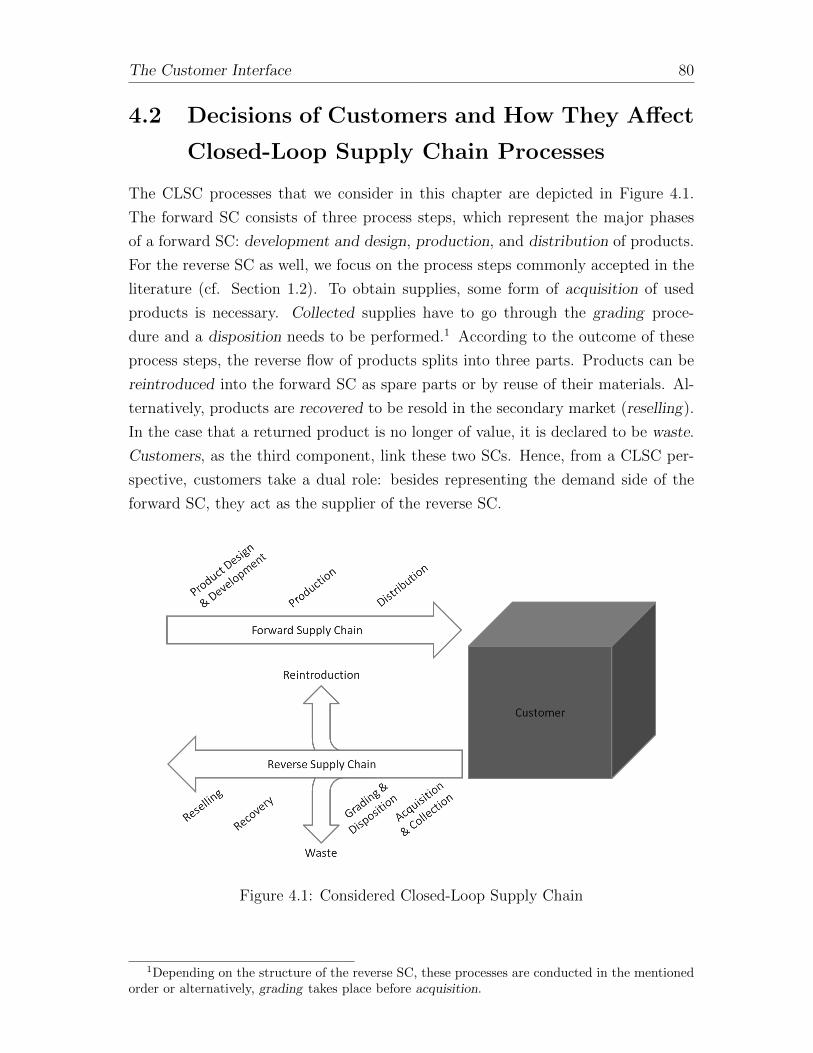
The Customer Interface 80
4.2 Decisions of Customers and How They Affect
Closed-Loop Supply Chain Processes
The CLSC processes that we consider in this chapter are depicted in Figure 4.1.
The forward SC consists of three process steps, which represent the major phases
of a forward SC: development and design, production, and distribution of products.
For the reverse SC as well, we focus on the process steps commonly accepted in the
literature (cf. Section 1.2). To obtain supplies, some form of acquisition of used
products is necessary. Collected supplies have to go through the grading proce-
dure and a disposition needs to be performed.1 According to the outcome of these
process steps, the reverse flow of products splits into three parts. Products can be
reintroduced into the forward SC as spare parts or by reuse of their materials. Al-
ternatively, products are recovered to be resold in the secondary market (reselling).
In the case that a returned product is no longer of value, it is declared to be waste.
Customers, as the third component, link these two SCs. Hence, from a CLSC per-
spective, customers take a dual role: besides representing the demand side of the
forward SC, they act as the supplier of the reverse SC.
Figure 4.1: Considered Closed-Loop Supply Chain
1Depending on the structure of the reverse SC, these processes are conducted in the mentionedorder or alternatively, grading takes place before acquisition.

The Customer Interface 81
Figure 4.2: Stages of The Customer Acquisition Decision (based on Homburg, 2012,p.104)
To achieve an efficient management of CLSCs, we need to know what happens
during the use phase at the customer. To bring light to this “black box”, we describe
a customer’s usage and return behavior via the decisions that a customer makes.
In the following subsections, we discuss how these customer decisions affect the
considered CLSC processes and identify coordination needs.
To be able to provide appropriate incentives to the customers, it is of relevance
to know how a customer benefits from a product, its usage and a potential return.
Based on literature evidence, we therefore also describe how a customer is expected
to benefit from these decisions, when we introduce customer decisions. We will
return to these customer benefits when addressing the mechanisms that can be used
to the facilitate identified coordination issues at the customer interface (Section 4.4).
First of all, a customer needs to decide to acquire the offered, new product. In
fact, the customer’s acquisition decision needs to be regarded as a process (Hom-
burg, 2012). In Figure 4.2, we depict the four stages of which this process consists.
After the decision to acquire any product (Stage 1) and the choice of a certain
product category (Stage 2), the customer chooses an actual product from the of-
fered alternatives on the market. Based on the assumption of customers as rational
decision makers, in the marketing literature microeconomic utility based selection
models are common to explain the customer’s product choice theoretically. Partic-
ularly important thereby is the model introduced by Lancaster (1966): based on its
utility function, the decision maker assesses characteristics of a product instead of
the product as a whole. Hence, in traditional forward SCs, the customer’s acquisi-
tion decision is influenced by the possibility (with respect to monetary limitation),
the need to use the product, and the characteristics of the offered product. In a
CLSC context, besides the characteristics influencing the value of using a product,
customers extent their valuation of a product to the characteristics that come into
play after the usage phase. This reselling value needs to be taken into account in a
customer’s acquisition decision (Debo et al., 2005; Oraiopoulos et al., 2012). Upon
the acquisition, the product is handed over to the customer and the usage phase
starts.
The Customer Interface 82
The end of the usage phase is represented by the - as we call it - customer’s
disposition decision. A customer decides whether to return a product or not, and
in the case of returning the product, to whom the product is given. Reverse SC
literature distinguishes between returning the product to the OEM or a third-party
reprocessor (e.g. Ferguson and Toktay, 2006). Trading activities between (private)
customers e.g. via internet platforms and donation represent two further customer
disposition options. Assuming the customer has no further interest in the product
in terms of usage, the customer’s different disposition options offer value to the cus-
tomer according to his individual characteristics, which can be seen as his individual
“mental book value” (Ray et al., 2005) or “willingness to sell” (Gonsch, 2014).
Related to the customer’s disposition decision is his decision how long to use the
acquired product. Following Fisher’s (1997) distinction of functional and innovative
products, depending on the product type, the benefits that a customer takes from a
product during the usage phase are either rather stable or slowly decreasing in the
case of functional products, decreasing quickly in the case of innovative products.
Furthermore, the usage of a product may vary from customer to customer in
several aspects, which usually cannot be observed by other actors than the customer
himself. First to mention, the intensity with which a product is used, which usually
affects the condition of the product. Hence, the more a customer benefits from
a product, the higher the usage intensity and the greater the wear and tear of the
product. Some customers may decide to use (maintenance) services during the usage
phase. This decision can affect the benefits in both ways. On the one hand, the
customer usually cannot use the product during the service; on the other hand, he
can benefit from an improved product with an increased reselling value (Oraiopoulos
et al., 2012). Thus, negative and positive impacts depend on the service type and
the way in which the product itself is affected. Another customer decision is related
to complementary products, like toner cartridges for printers. The usage of such
complementary products usually enables the further use of the original product and
thereby increases a customer’s benefits. However, the costs of such complementary
products need to be taken into account as well.
Summarizing, to bring light to the “black box”, we discuss the effects of the
following six decisions on the above CLSC processes:
• Customer acquires the product
• Customer’s disposition decision
• Duration of usage phase

The Customer Interface 83
• Intensity of usage
• Demand for (maintenance) services
• Demand for complementary products
This list is neither provided in a particular order nor presumed to be complete.
However, the chosen decisions provide a profound basis on which to derive coordi-
nation needs at the customer interface. Hence, at the end of this section, we will be
able to answer our research question.
4.2.1 Customer Acquires the Product
Customers’ acquisition decision determines the quantity of products delivered to
customers and therefore the generated profits of the forward SC. Extending the
setting to a CLSC, the acquisition quantity has an additional impact. The quantity
acquired in the first period represents the upper bound of the available supplies in
the future, after-usage period (Debo et al., 2005).
The value-generating usage of these supplies is twofold in our example. Either re-
turned products are recovered and generate profits on the secondary market or their
components and materials are reintroduced into the forward SC as inputs, which
usually results in production cost savings. Thus, taking for example a smartphone,
the phone can either be dismantled and included materials such as rare earth met-
als recycled and used in the production of new phones or be repaired or refurbished
and sold to customers with a lower willingness to pay. However, the question arises
of whether these recovered smartphones cannibalize the new product demand (e.g.
Ferguson, 2009; Guide and Li, 2010).
This results in a crucial trade-off (Figure 4.3): from a long-term CLSC perspec-
tive, on the one hand, the amount of available supplies should be sufficiently large to
fulfill the demand for recovered products and the producing actors want to benefit
from materials and components that are less expensive than new ones. On the other
hand, there might be the necessity to limit sales to the primary market artificially
and thereby limit the available supplies of the reverse SC to avoid the cannibaliza-
tion effect. It is therefore of interest to balance the profits of the primary and the
secondary market and thereby consider the customer’s acquisition decision, which
is affected by the product attributes.
The aim to balance the primary and the secondary market profits may be further
complicated due to independent reprocessing companies that potentially enter the

The Customer Interface 84
Figure 4.3: Effects of the Customers Product Acquisition Decision
market. This damages OEMs in two ways. First, reprocessed products sold by com-
petitors cannibalize the OEM’s new products sales, which additionally impacts on
the OEM’s profits. Second, the OEM cannot benefit from investments in reusability
attributes (Ferguson and Toktay, 2006).
Hence, as a first coordination need at the customer interface, we derive: Incen-
tivize the CLSC optimal acquisition quantities to balance the profits of the primary
and the secondary market.
4.2.2 Customer’s Disposition Decision
While the product acquisition decision represents the beginning of the usage, the
customer’s disposition decision represents its end. One disposition option is to keep
the product, which means that there is no reverse flow originating from this cus-
tomer. Given that a customer decides to return his product, we distinguish further
disposition options:
• Direct disposal by the customer
• Donation without any value-adding activity
• An interaction between customers takes place without any value-adding activ-
ity

The Customer Interface 85
Figure 4.4: Effects of the Customer’s Disposition Decision
• The product is provided as supply for the reverse SC. In this case, which actor
it is submitted to is of interest:
– OEM
– Third-party remanufacturer
Due to these multiple disposition options, there is uncertainty with respect to
the amounts of returned products that reach the reverse SC and to which actor they
are actually sent. In Figure 4.4, we indicate which CLSC processes are affected by
this customer decision.
One issue is that due to the quantity uncertainty, the capacity planning of re-
verse SC activities is complicated. Additionally, uncertain return volumes affect the
disposition decision and thus, the available amounts for reselling and reintroduction
into the forward SC are affected (Fleischmann et al., 2010). We take for example
the CLSC of a notebook and assume that our reverse SC faces some market demand
for recovered notebooks, which depends on the price as well as the offered quality.
To receive supplies, current users (= customers) need to be incentivized to return
their used notebook (Gonsch, 2014). By doing so, incentives + reprocessing cost ≤market price. Otherwise, reprocessing activities are not beneficial for the reprocess-
ing actor. However, current users need to be convinced to return their notebook to

The Customer Interface 86
Figure 4.5: Effects of the Customer’s Decision on the Duration of the Usage Phase
assure supplies to satisfy the demand. As long as the customer has multiple dispo-
sition options, he needs to be influenced to make the optimal disposition decision
from a CLSC perspective. When designing the incentive for the customer, both
sides therefore have to be considered, the customer (=supply) and the demand side,
meaning what can be gained on the secondary market or saved in the production of
new products. This means that a pricing decision is central.
The arising coordination need is to incentivize the customer to choose the CLSC
optimal disposition decision to match the supply quantities with the demand.
4.2.3 Duration of Usage
Highly related to the customer’s disposition decision is his decision on the duration
of the usage phase. However, the effects of the two decisions differ from each other.
Assuming that a customer returns his product to the SC under consideration, the
decision on the duration of the usage phase determines the timing of a return, while
the effects of the decision actually to return a product concern the quantity.
The effects of the customer’s decision on the duration of the usage phase are
summarized in Figure 4.5. Usually the customer’s decision is unknown to all the
other CLSC actors and therefore the timing of returns is uncertain a priori. This
uncertainty especially affects the planning of resources, both in the forward and in

The Customer Interface 87
the reverse SC. We identify four effects on the CLSC processes related to the uncer-
tain timing of returned products. First, the capacities for the reverse SC activities
are affected. As an example, we again consider the case of returned smartphones.
Due to the high depreciation rate, it is necessary to conduct the reverse processes in
a short period of time. However, as the timing is uncertain a priori, the reverse SC
needs to build up high capacities to be able to handle all the returned units even in
the case of return peaks. Second, reselling is affected due to uncertain availability
of the recovered products. Third, the planning of the required new supplies in the
forward SC is affected (Ketzenberg et al., 2006). Producers face a trade-off between
relatively cheap but uncertain materials and components that can be obtained from
used products and more expensive but rather reliable new supplies: an aspect that
is of special importance in the case of used components are used as spare parts. A
customer who wants, for example, his car repaired will not be willing to accept long
waiting times due to unavailable supply, but instead will go to another repair shop.
Fourth, the planning of transportation is affected. The joint delivery of products
and the collection of used products in a CLSC setting provides the opportunity to
save transportation costs (Fleischmann et al., 2009). However, the complexity of
the planning tasks increases due to the uncertainty regarding whether the event of
a product return coincidences with the necessity to deliver something.
Furthermore, the duration of the usage phase and thus the timing of the return of
a product (may) affect the attractiveness of return flows. This can be seen from two
perspectives. First, it depends on whether an actor has empty capacities for reverse
flows - this is related to the aforementioned planning issues. Second, there needs to
be a demand for recovered products and respectively used parts and materials.
On the one hand, there is the customer who requires and therefore benefits from
the usage of a product for some time. On the other hand, there are the other CLSC
parties involved in the reprocessing activities, who require supplies to fulfill their
demands at a given point in time. The effects on the CLSC processes introduced
above result in the coordination need to incentivize the CLSC optimal duration to
manage the timing of returns according to the available capacities and the required
supplies to satisfy the demand.
4.2.4 Intensity of Usage
Next, we consider the question of how CLSC processes are affected by the customer’s
decision on the intensity of usage (Figure 4.6). The intensity of usage impacts on the
quality of a product. The more intense the usage and the less carefully a product is
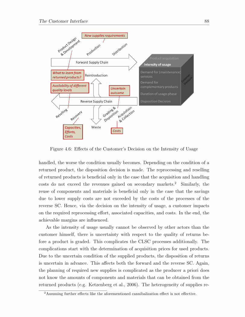
The Customer Interface 88
Figure 4.6: Effects of the Customer’s Decision on the Intensity of Usage
handled, the worse the condition usually becomes. Depending on the condition of a
returned product, the disposition decision is made. The reprocessing and reselling
of returned products is beneficial only in the case that the acquisition and handling
costs do not exceed the revenues gained on secondary markets.2 Similarly, the
reuse of components and materials is beneficial only in the case that the savings
due to lower supply costs are not exceeded by the costs of the processes of the
reverse SC. Hence, via the decision on the intensity of usage, a customer impacts
on the required reprocessing effort, associated capacities, and costs. In the end, the
achievable margins are influenced.
As the intensity of usage usually cannot be observed by other actors than the
customer himself, there is uncertainty with respect to the quality of returns be-
fore a product is graded. This complicates the CLSC processes additionally. The
complications start with the determination of acquisition prices for used products.
Due to the uncertain condition of the supplied products, the disposition of returns
is uncertain in advance. This affects both the forward and the reverse SC. Again,
the planning of required new supplies is complicated as the producer a priori does
not know the amounts of components and materials that can be obtained from the
returned products (e.g. Ketzenberg et al., 2006). The heterogeneity of supplies re-
2Assuming further effects like the aforementioned cannibalization effect is not effective.

The Customer Interface 89
sults in highly uncertain reprocessing efforts, which in turn complicate the capacity
planning (e.g. Fleischmann et al., 2010). Furthermore, due to the uncertain yield
of supplies, the reprocessing costs are uncertain a priori. This makes it difficult to
predict how many reprocessed products of which quality can be offered to secondary
customers.
These effects on the CLSC processes result in the coordination need to incentivize
the CLSC optimal intensity of usage to align the received and the required quality
of returned products.
Another effect occurs less due to the uncertain condition of returned products
but rather due to the unobservable handling causing this uncertainty. Once products
are returned to the OEM, one advantage of reverse flows can be seen in the chance
to gather additional information for new product development or the improvement
of the current product versions. However, OEMs are only able to draw conclusions
from the observed condition, in the case that they know how the product was used
by the customer. Hence, it is of importance to establish a relationship between the
reprocessing OEM and the customer to establish transparency with regard to the
handling of the product.
4.2.5 Demand for (Maintenance) Services
While the aforementioned decisions affect the physical flow or the product itself, the
following two decisions impact on the availability of information. This is less about
causing uncertainty, but rather about gathering information on other customer de-
cisions.
We start with a customer’s decision to demand (maintenance) services and show
which kind of information can be gathered in Figure 4.7. Let us take a copying
machine for example, which is currently used by a customer. During his usage
phase, the customer may request maintenance due to a problem that has occurred
or according to a predetermined inspection on a regular basis. This interaction with
the customer offers the opportunity to access information on both the way in which
the copying machine is used and the condition of the components, like hardware or
included technology. Furthermore, it may be possible to obtain additional informa-
tion, such as whether the customer intends to return the copying machine and if
so, when this will probably be. This means that the forecasting of returned prod-
ucts with respect to timing and quality becomes more accurate. Thus, it is possible
to decrease the aforementioned planning complexities and manage the CLSC more
efficiently.

The Customer Interface 90
Figure 4.7: Effects of the Customer’s Decision to Demand (Maintenance) Services
Moreover, customers can be asked whether the handling of the copying machine
is in accordance with their expectations, whether they have observed any problems,
and whether they have ideas for further improvements. Thus, due to the interaction
with customers, it is possible to identify problems and potentially adapt the current
product versions or to improve future versions of the product.
One aspect to add here is that information gathered during the service activi-
ties needs to be accessible by the actor responsible for the aforementioned CLSC
processes, namely on the one hand, the OEM for improvement of future design and
production processes and, on the other hand, the actor who is responsible for the
reverse flow activities. Otherwise, the actor responsible for the service activities can
take advantage of the information obtained either by selling the information or by
avoiding other parties entering the market.
4.2.6 Demand for Complementary Products
Similar to the aforementioned decision, the demand for complementary products
represents a decision that provides information on other decisions rather than caus-
ing uncertainty itself (Figure 4.8). As an illustrative example we choose a printer
with toner cartridges as complementary products. In the case that a reprocessing
actor can access the information on a specific customer buying toner cartridges, he
can learn two things. First, due to the frequency of the orders of toner cartridges, it

The Customer Interface 91
Figure 4.8: Effects of the Customer’s Decision to Demand Complementary Products
becomes more transparent how many printouts are being made; thus, information
on the intensity of the usage can be gathered. Second, buying a new toner cartridge
implies that a customer will most likely use the printer for a further length of time.
In combination with the information on the frequency of purchases, information on
the further minimum duration of the usage, and thus the timing of the return, is
provided.
Hence, similar to the service demand, the reprocessing actor is able to gather
information that enables him to manage the CLSC activities and resources more
efficiently. It is less the need for coordination, but rather the necessity to offer these
complementary products and make the relevant conclusions that can be derived
from the information that customers usually provide on a voluntary basis or that
are enabled due to information systems becoming more and more sophisticated.
Both the demand for maintenance services and the demand for complementary
products provide the opportunity to gather information; however, this information
should not be taken for granted. Thus, the uncertainty decreases but still exists.
In Table 4.1, we provide an overview of the effects of the customer decisions
discussed in previous sections.

The Customer Interface 92
Design
&Develop-
ment
Production
Distrib
ution
Collection
& Acquisition
Gradin
g&
Disposition
Recovery
Reintro-
duction
Rese
llin
g
Product
acquisi-
tion
pro
du
ctatt
rib
ute
sd
eman
dca
n-
nib
aliza
tion
max.
availab
leam
ou
nt
max.
availab
leam
ou
nt
Custom
er’s
disposi-
tion
decision
requ
ired
new
sup
plies
ince
nti
ves
,ca
paci
tyca
paci
tyca
paci
typ
rice
pri
ce
Duration
ofusa
ge
phase
requ
ired
new
sup
plies
tran
sport
ati
on
tran
sport
ati
on
,ca
paci
ty,
att
ract
iven
ess
of
retu
rnfl
ow
s
cap
aci
tyca
paci
tyavailab
ilit
yavailab
ilit
y
Inte
nsity
ofusa
ge
pro
du
ctim
pro
vem
ent
requ
ired
new
sup
plies
acq
uis
itio
nco
sts
un
cert
ain
ou
tcom
eeff
ort
s,ca
paci
ty,
cost
Tab
le4.
1:Sum
mar
yof
Eff
ects
ofC
ust
omer
Dec
isio
ns
The Customer Interface 93
4.3 Identified Coordination Needs at the Custom-
er Interface
In Figure 4.9, we cluster the customer decisions considered in the previous sections
according to two insights. First, the customer decisions can be divided into decisions
causing coordination needs at the customer interface and decisions that facilitate the
customer interface as they provide the opportunity to gather information on future
reverse product flows. Second, the effects of the decisions causing coordination
needs at the customer interface can be clustered into quantity-, quality-, and timing-
related. Each of the four decisions can be clearly assigned to one of these categories
and accordingly can be seen as their drivers:
• While a customer’s acquisition decision determines the total amount of poten-
tial future supplies, a customer’s disposition decision determines the amount
of supplies of a certain reverse channel. Therefore both decisions affect the
CLSC processes via the quantity.
• The decision on the intensity of usage affects several CLSC processes via the
quality of return flows.
• The decision on the duration of usage affects several CLSC processes via the
timing of return flows.
Concerning our research question, we can state that quantity-, quality-, and timing-
related coordination needs exist.
The decisions facilitating the customer interface are not assigned to further sub-
categories. Both the customer decision on maintenance services and the one on com-
plementary products help to gather information on the quality and on the timing of
the return flows. Furthermore, on an aggregated level, they provide information on
the quantities of reverse flows.
In Table 4.23, we indicate which CLSC processes are affected by the customer
decisions considered and state the identified coordination need for each decision. In
total, we identified five coordination needs at the customer interface:
• Incentivize the CLSC optimal acquisition quantities to balance the profits of
the primary and the secondary markets.
3This table represents an extension of Table 4.1. However, due to clarity reasons, we indicatewhich CLSC processes are affected by a customer decision with an “x” instead of stating the actualeffect.

The Customer Interface 94
Figure 4.9: Clustered Summary of Customer Decisions
• Incentivize the customer to choose the CLSC optimal disposition decision to
match the supply quantities with the demand.
• Incentivize the CLSC optimal duration of usage to align the end of usage phase
with the timing of the demand for reprocessed products.
• Incentivize the CLSC optimal intensity of usage to align the received and the
required quality of returned products.
• Incentivize transparency with regard to the intensity of usage to enable product
improvements.
In their acquisition decision, customers take into account the attributes of a
product. Hence, by the determination of these attributes, the first coordination
need to incentivize the CLSC optimal acquisition quantities to balance the profits
of the primary and the secondary markets can be addressed. Among others, a
product’s attributes determine whether a product is reusable at all. Thus, the
determination of the attributes of a product is of a strategic nature. We cover this
issue in Section 4.4.1.4
Turning to the remaining coordination needs, these are more about initiating
reverse flows in sufficient quantities, with the perfect timing, or of the CLSC op-
4When addressing the other coordination needs, the product’s attributes are assumed to be givenand the forward SC process design and development is excluded from the further consideration.

The Customer Interface 95
timal quality to satisfy the demand for reprocessed products (=reintroduction and
recovery). In the summary of effects of customer decisions (Table 4.1) we see that
the only identified effect of customer decisions on the forward SC process distribu-
tion concerns the joint transportation of new and returned products. Due to the
subordinated role of transportation in comparison to all other effects identified, we
exclude this effect for a moment.
Revisiting Table 4.2, we make an important observation. Except for the reintro-
duction, all the processes considered are affected by quantity, timing, and quality.
This implies that the underlying goal of matching supply and demand can therefore
only be achieved by mechanisms that take into account the three customer deci-
sions simultaneously. Otherwise, driver(s) of uncertainty are potentially neglected
and a full picture of real-world problems cannot be provided. Hence, the identified
coordination needs at the customer interface can be summarized as:
The initiation of reverse flows in sufficient quantity, of CLSC optimal quality, to
satisfy the demand for reprocessed products at a given time.
We discuss mechanisms that could potentially satisfy this coordination need in
Section 4.4.2.
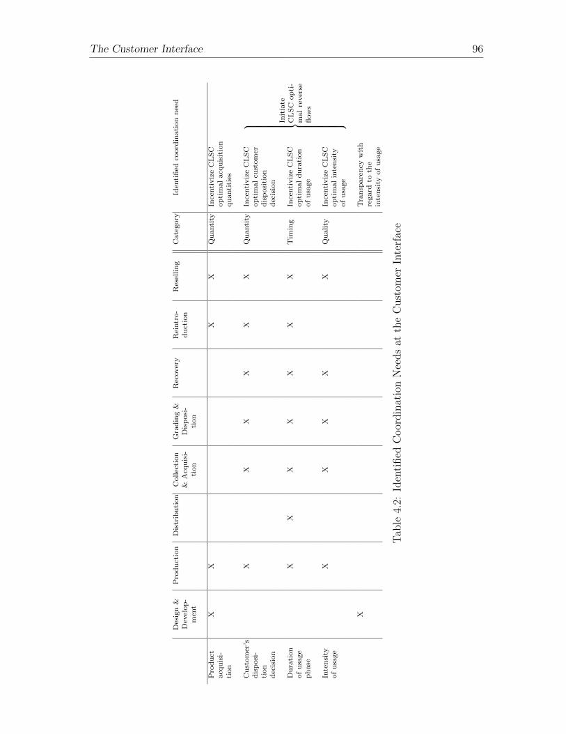
The Customer Interface 96
Des
ign
&D
evel
op
-m
ent
Pro
du
ctio
nD
istr
ibu
tion
Collec
tion
&A
cqu
isi-
tion
Gra
din
g&
Dis
posi
-ti
on
Rec
over
yR
eintr
o-
du
ctio
nR
esel
lin
gC
ate
gory
Iden
tified
coord
inati
on
nee
d
Pro
du
ctacq
uis
i-ti
on
XX
XX
Qu
anti
tyIn
centi
viz
eC
LS
Cop
tim
al
acq
uis
itio
nqu
anti
ties
Cu
stom
er’s
dis
posi
-ti
on
dec
isio
n
XX
XX
XX
Qu
anti
tyIn
centi
viz
eC
LS
Cop
tim
al
cust
om
erd
isp
osi
tion
dec
isio
n
Init
iate
CL
SC
op
ti-
mal
rever
sefl
ow
s
Du
rati
on
of
usa
ge
ph
ase
XX
XX
XX
XT
imin
gIn
centi
viz
eC
LS
Cop
tim
al
du
rati
on
of
usa
ge
Inte
nsi
tyof
usa
ge
XX
XX
XQ
uality
Ince
nti
viz
eC
LS
Cop
tim
al
inte
nsi
tyof
usa
ge
XT
ran
spare
ncy
wit
hre
gard
toth
ein
ten
sity
of
usa
ge
Tab
le4.
2:Id
enti
fied
Coor
din
atio
nN
eeds
atth
eC
ust
omer
Inte
rfac
e

The Customer Interface 97
4.4 Mechanisms to Coordinate the Coordination
Issues at the Customer Interface
We were able to identify two coordination needs at the customer interface originat-
ing from the customer decisions considered. In this section, we discuss how these
coordination needs can be addressed. In this regard, we provide an overview of the
potential sources of useful coordination mechanisms and discuss the most promising
ones. Due to coordination, the maximization of CLSC benefits will be achieved.
In this regard, we need to take into account both the customer benefits and the
profit-maximization objective of all the other actors involved.
4.4.1 Incentivize the Closed-Loop Supply Chain Optimal
Acquisition Quantities
A customer’s acquisition decision is influenced by the buying opportunity, the neces-
sity to use the product, and the attributes of an offered product (Homburg, 2012).
In a CLSC context, we need to consider the attributes that come into play after the
usage phase (Debo et al., 2005; Oraiopoulos et al., 2012).
Consider a customer decides to acquire a smartphone. In terms of the customer
acquisition decision process (Figure 4.2), the customer is on stage three “Product
Choice” and needs to choose a particular product. Among the offered products, the
customer chooses based on the his valuation of certain product attributes (Lancaster,
1966), such as features, performance, and price. In addition to these characteristics
affecting the customer valuation during the usage phase, customers potentially think
of what happens after their usage of the phone. Some customers may want to
sell their used smartphone when they acquire a new one. Thus, the quality and
durability of, for example, the battery become relevant to assure some reselling value.
Furthermore, a major product characteristic in a CLSC context is its reusability.
Reusability determines whether a product can be reprocessed in later periods at
all. Different degrees of reusability affect the ease of reverse flow activities. Besides
these considerations of an OEM, the environmental perspective of reusable products
is relevant to the acquisition decision of “green customers”.
Taking a CLSC perspective, diverse impacts need to be considered when deter-
mining a product’s attributes:
1. The customer’s acquisition decision itself; thus, the sales volumes of the new
product are affected.

The Customer Interface 98
2. Cannibalization of the new product demand due to reprocessed products.
3. Increased production costs due to enhanced product attributes.
4. Reusability simplifies the reverse flow of products and cost savings can be
achieved.
Thus, it comes down to the decision on the design of a product. The paper by
Debo et al. (2005) described in the general literature review (Section 2.2) addresses
the key managerial issue of whether it is profitable to produce a reusable product.
Besides the influence of cost structures, the authors explicitly address the issue
“How the optimal level of remanufacturability5 changes as a function of the customer
profile” (p.1199). In their model, customers are characterized in terms of willingness
to pay for new as well as willingness to pay for reprocessed products. Their results
show that the optimal choice of a product’s reusability depends on the market
structure. In case of a diverse market, a high reusability level is optimal, whereas in
case of “markets with high concentration of customers on either the high end or the
low end, the optimal remanufacturability level is low”(p.1200). These results offer
an excellent basis for the optimal choice of product attributes to balance the profits
of the primary and the secondary market depending on the customer structure.
In the following, we assume that the decision on the reusability of a product is
given and address the second coordination need.
4.4.2 Initiating Closed-Loop Supply Chain Optimal Reverse
Flows
From our analysis of the effects of customer decisions on CLSC processes, we de-
rived that there are interdependencies of the effects of the customer decision on the
disposition, duration, and intensity. These interdependencies require joint consid-
eration and the resulting coordination need can be summarized as the initiation of
reverse flows in sufficient quantity, of CLSC optimal quality, to satisfy the demand
for reprocessed products at a given time. Against the background of this coordina-
tion need, we briefly revisit the concepts of active product acquisition management,
leasing, and trade-in programs introduced in Section 4.1.
The aim of active product acquisition management is to receive products of the
right quality, in the right quantity, at the appropriate time to satisfy the demand -
which is equal to the identified coordination requirement. However, an underlying
assumption of these models is that the supply of returned products is restricted by
5This corresponds to our term “reusability”

The Customer Interface 99
the amount of products sold in previous period(s) only. The effects of customer
decisions on the availability of supplies are not included. This means that the
customer interface is not covered.
To the best of our knowledge, the recent publication by Gonsch (2014) is the
only work that includes direct customer interaction in a CLSC context. Assuming
that customers do not “(. . . ) simply want to get rid of their used products without
expecting any compensation for them (. . . )” (p.715), he addresses the benefits of
bargaining instead of posted prices. Product owners return their product if and
only if the price received is higher than their willingness to sell. A product owner’s
valuation is uniformly distributed in the interval [α∗ price paid, price paid] with
α ∈ [0,1]. The profit-maximizing OEM chooses his maximum bargaining price and
thereby manages the received quantities in the current period. The author covers the
customer’s disposition decision and, due to the formulation as a single-period model,
to some extent the customer’s decision on the duration of usage. However, as it is
assumed that all the products received have the same input quality, the heterogeneity
of customers’ decisions on the intensity of usage is not included. Furthermore, the
focus is on the maximization of an OEM’s profit and not on CLSC optimization.
Leasing is a popular take-back mechanism, especially in a B2B context, because
lessors as well as customers can take advantage of leasing. While customers benefit
from increased flexibility to update their equipment frequently, from a CLSC per-
spective, the advantage of decreased timing and quantity uncertainty needs to be
highlighted. Although a leasing duration is usually agreed, a customer is not forced
to return his product at the end of the leasing period. This results in a certain
level of uncertainty (Guide, 2000). This circumstance, in which a customer may not
return a product after a leasing period, is incorporated into the work neither by
Agrawal et al. (2012) nor Robotis et al. (2012). Agrawal et al. (2012) assume a fixed
usage phase of one period. After this period, the product is - depending on whether
the leasing or the selling strategy is followed - either returned to the leasing com-
pany or sold to other customers or respectively recycled by the primary customer.
Robotis et al. (2012) determine the optimal duration of leasing contracts. They also
do not consider the customer’s decision, but assume that the same leasing duration
is valid for all customers and that at the end of the leasing contract, the products
are collected by the OEM. Leasing is seen as an attractive mechanism to initiate
reverse flows (Souza, 2013). However, as the previous models do not incorporate
the customer interface, the effects of customer decisions have been neglected.
Finally, we introduced trade-in programs as a take-back mechanism found in the
previous literature. As mentioned, the idea is to offer a rebate to customers to induce

The Customer Interface 100
product owners to replace their current product with a new one. In a CLSC context,
two papers consider this mechanism. Ray et al. (2005) suggest optimal pricing and
trade-in rebates based on the age profile of the products in use. While this age-
structure-based rebate matches the customer’s willingness to sell quite well, both
return revenues and cost savings for reverse and forward SC actors usually rather
depend on the quality of a product - which is influenced by the customer’s decision on
the usage intensity. This customer decision (and its resulting effects) is not included
in their analysis. Li et al. (2011) suggest a customer segmentation method that
may be used by the OEM (the authors consider a company in the high-tech sector)
to offer segment-specific trade-in rebates. Customers are segmented according to
their reliability, which is derived from a comparison of previous customer signals
and actually returned products. The customer signals are observed via a so-called
return merchandise authorization form, which usually includes information on the
name of the product and the customer, as well as the quantity and condition of the
trade-in product. Due to the customer segmentation method, reprocessing actors
are able to forecast the quality of future returns. However, the timing as well as the
quantity remain unknown. This is because of the time windows that are commonly
offered to customers. Due to this period of up to 120 days, the timing of returns
remains uncertain to some extent. Furthermore, it is not given that the announced
products are returned at all. Hence, the amount actually received is uncertain as
well.
As summarized in Table 4.3, the previous developments towards an actively man-
aged return process cover some of the identified customer decisions but so far none
of the concepts provides an integrated mechanism. In contrast to the coordination
need at the customer interface covered in Section 4.4.1, the coordination of reverse
flows has not been covered in the previous literature. To clear the way for such a
mechanism jointly coordinating the quantity, quality, and timing of reverse flows,
we discuss potential “candidates” in the following. By coordination, the customer’s
benefits as well as the other actors’ profits will be optimized. We provide a summary
of the effects of customer decisions on the CLSC processes as well as the benefits
that a customer receives from his decisions in Figure 4.10.
Avoiding unnecessarily reinventing the wheel, we draw on the aforementioned
take-back mechanisms as well as on the coordination concepts introduced in the
forward SC literature. While we introduce ideas and focus on a conceptual level,
future projects may focus on how actually to choose contract parameters/design
mechanisms, depending on different context settings.

The Customer Interface 101
Figure 4.10: Customer Decisions - Summary of Effects on Closed-Loop Supply ChainProcesses and How Customers Benefit
Strategies Based on Take-Back Mechanisms
We discuss potential extensions/modifications of the two strategic take-back con-
cepts, leasing and trade-in, to take into account the customer interface, in the fol-
lowing.
The current leasing considerations do not incorporate the customer interface.
This results in a certain extent of uncertainty with respect to the quantity and
timing of return flows - both complicating the planning of CLSC activities and
capacities. Furthermore, the heterogeneity of returned products with respect to
the quality is not included, which increases the planning complexity further. To
establish a CLSC optimal reverse flow, these disadvantages need to be overcome.
In fact, the timing and the quality of the returned products should be stipulated
and in the case that a customer does not meet these agreed-on stipulations, penalties
are incurred. Taking this as an assumption, the heterogeneity of supplies is avoided
and the planning complexity is no longer greater than in a forward SC setting. How-
ever, to derive CLSC optimal stipulations with regard to the leasing duration and
the condition of end-of-lease products as well as to derive the associated penalties,
both the customer benefits and the profit maximization of all the other actors need
to be taken into account. The introduction of penalties represents a crucial change
of the current concept and its impact on customer’s acquisition decision has to be
taken into account.
In contrast to leasing, there are no contractual agreements between the actor

The Customer Interface 102
Dispositiondecision (Quantity)
Duration of usage(Timing)
Intensity of usage(Quality)
Productacquisitionmanagement
Gonsch (2014) affected by priceLeasing
Agrawal et al.(2012)
decreaseduncertainty
decreaseduncertainty
Robotis et al.(2012)
decreaseduncertainty
decreaseduncertainty
Trade-in
Ray et al.(2005)
affected by rebate age-dependent
Li et al.(2011)
time window time window forecasts based oncustomersegmentation
Table 4.3: Coverage of the Customer Interface by Previous Literature
offering a trade-in program and the product user. Hence, penalties are an ineligible
lever here. The customer segmentation method developed by Li et al. (2011) makes it
possible to forecast the quality of returns. However, timing and quantity uncertainty
is still an issue. Therefore, the customer’s disposition decision and his decision on
duration have to be considered.
Whether a product is handed in at all represents a customer’s disposition deci-
sion. A customer can choose between different alternatives (Section 4.2.2). Usually
a product owner will not keep, donate, or dispose of his current product if the price
that is offered is higher than his willingness to sell. This results in three remaining
disposition options, between which the customer can choose. He can return the
product to the OEM, sell it to a third-party reprocessor, or sell it to other cus-
tomers. Hence, competition for the used products needs to be taken into account
when determining the offered trade-in rebate.
Usually, if a customer accepts a concrete trade-in offer, he does not really use
the current product anymore and the timing decision is less affected by the bene-
fits from the product itself than by the “burden” actually to hand in the product.
Thus, to receive the product in a timely manner, bonus payments in addition to the
agreed on trade-in conditions may be an idea to decrease the timing uncertainty.

The Customer Interface 103
However, the trade-off between bonus payments and costs savings due to decreased
uncertainty needs to be taken into account.
Strategy Based on Forward Supply Chain Mechanisms
As an alternative to these take-back mechanisms, the coordination concepts intro-
duced in the forward SC literature may offer mechanisms that can be adapted to the
CLSC setting. While the mechanisms (introduced in Section 2.1) focus on demand
uncertainty (Arshinder et al., 2011) our coordination need mainly originates from
uncertainties with regard to the supply side. However, in line with the suggestion of
Debo et al. (2004), to use existing forward SC theory to address coordination issues
faced in reverse SCs, we use the existing coordination mechanisms as starting point.
We reviewed mechanisms that either coordinate settings of unaligned incentives
of decision makers or both unaligned incentives and information asymmetries. As
we have seen, customers acting as the demand as well as the supply side possess
exclusive information that results in supply uncertainties. Hence, a mechanism is
required that addresses both unaligned incentives and information asymmetries. In
this regard, we reviewed the agency literature and technology-driven joint decision-
making initiatives. While the first requires assumptions on and the analysis of cost
structures and distributions of preferences and so on, the latter can be discussed on
a higher, rather conceptual level - which is the matter considered in this section.
Our choice is further driven by the rapidly growing diffusion of ICT. This arouses
our interest in a concept using the opportunities that technological support provide.
Among the technology-enabled mechanisms, VMI is an accepted industry prac-
tice and one of the most discussed joint decision making initiative (Waller et al.,
1999; Pfohl, 2002). This raised our interest in adapting the idea of VMI to a CLSC
setting. In the following, we will suggest how to adapt the concept to coordinate
the customer interface with regard to the initiation of CLSC optimal reverse flows.
In the original setting, the retailer’s decision on timing and quantity is shifted
to the supplier. While the supplier benefits from avoidance of the bullwhip effect,
retailers benefit from reduced ordering and monitoring costs. Transferring the idea
to our setting, the decision to initiate reverse product flows needs to be shifted
from the customer to the reprocessor. Such a shift enables the reprocessing actor to
receive (based on his demand forecasts of new and recovered products) the required
amounts of returned products at the optimal quality at the perfect point in time.
This raises two questions:
1. How does a customer benefit from shifting his decisions and transferring his
private information to another actor?
The Customer Interface 104
2. Which information is required by the reprocessor?
We start with the latter question and discuss how to convince the customer to
transfer this information as well as shifting (some of) his decisions subsequently.
To begin with, the reprocessor requires demand information. Assuming that the
reprocessor sells directly to the primary and secondary markets, this information
is given by the reprocessor himself. Moreover, to fulfill the demands, supply and
information on supply is required. While for the production of new products supplies
are either in form of new parts and components or in the form of used products, the
single source of supply to fulfill the demand for recovered products is used products.
The planning of these supplies is complicated due to the heterogeneity of supplies
with respect to their condition and the available amount at a given point in time.
Depending on the reprocessing choice (reintroduction vs. recovery), distinct
planning issues arise. To achieve a profitable reintroduction of used products into the
new product production processes, the sum of the acquisition costs and reprocessing
costs needs to be lower than the costs of new supplies. Additionally, in order to plan
the required amount of new supplies, information on the available amount of used
materials and components is required.
Used products are the only supply for recovery. The condition of the products
is the major driver of the reprocessing costs. Together with the acquisition costs,
reprocessing costs determine the minimum reselling price to gain profits in the sec-
ondary market. The secondary demand is driven by these reselling prices and the
quantity of recovered products that is offered.
Planning is further complicated by the consideration of multiple periods. The
opportunity costs of initiating a reverse flow of a given quality now need to be taken
into account as well as the potential future condition of the product. The capacities
to conduct reprocessing activities now or in the future are a further driver of the
reprocessing costs.
To summarize, the reprocessor requires information on the current quality of a
product as well as information on the customer’s intended future intensity of usage.
In addition to this information, the reprocessor needs the power to initiate the
reverse flow of products of the required amount of products of a known quality at a
given point in time.
How does a customer benefit from shifting the decision to return his product
and transferring his information on intensity of usage to the reprocessor? While
the reprocessor facilitates his planning task due to the implementation of the idea of
VMI, the customer needs convincing arguments on the one hand to shift the decision
to return a product to the reprocessor and on the other hand to provide him with

The Customer Interface 105
quality information and in the case of multi-period considerations with his future
usage intensity intention.
Making a customer return his product at a given point in time obviously requires
some form of compensation, usually in form of a transfer payment or product ex-
change. With regard to information on quality, there are several possibilities. First,
the technological features of a product to track the usage come to mind. Thereby,
either the reprocessor is able to track the condition of a product continuously or the
stored data can be accessed during contact with the product during, for example,
maintenance servicing. The advantage of the integration of a data logger is that no
activity of the customer is required to transfer the information and the information
is not biased by the customer. On the other hand, adding technology increases the
production costs and customers potentially need to agree to their usage data being
accessed. Servicing represents a second possibility to gather quality information.
Either due to the possibly included data logger or via testing, the reprocessing actor
can gather information on the current condition. To gather this valuable infor-
mation, a reprocessing actor should encourage customers to request services on a
regular basis. How can this interaction with the customer be achieved? In general,
we distinguish two types of service requests: due to a problem or due to a service
arrangement, the latter being either enforced by law or voluntary. The reprocess-
ing actor does not need to incentivize the customers further to interact with him
in the case of a problem or if the service is enforced by law. However, incentives
are required if the service is voluntary. When designing the incentive scheme, the
reprocessing actor has to take into account that his benefits of decreased uncertainty
need to exceed the costs to incentivize the customers as well as the cost of provid-
ing the service. The incentives should therefore be based on the consideration that
customers take advantage of regular arrangements usually due to extended product
life, increased security, and a potentially increased reselling value due to documen-
tation of the services conducted. Nevertheless, they have to pay for the services and
hence need to be incentivized either due to the aforementioned aspect or due to the
incentives offered by the reprocessing actor. Another possibility to gather quality
information is the customer segmentation method suggested by Li et al. (2011). The
method is based on customer signals observed via return merchandise authorization
forms and allows for quality forecasts.
Taking a multi-period planning horizon, there is one remaining question con-
cerning how to gather information on the customer’s future decision on intensity of
usage. Here as well, one of the previously considered customer decisions can provide
insights. The customer’s decision on complementary products provides information

The Customer Interface 106
on the intensity of usage as well as on the intention to continue using the product.
We provided the example of toner and the insights with respect to intensity and
duration that one may obtain from the usage of complementary products such as
toner cartridges.
In this section, we discuss mechanisms to initiate CLSC optimal reverse flows.
We find that in previous modeling of take-back mechanisms, the customer’s disposi-
tion decision and his decisions on duration and intensity of usage are not considered
jointly. Furthermore, an OEM perspective is often taken. As a starting point to
overcome this weakness, we discuss strategies for including the customer in the con-
cept of leasing and trade-in programs. Additionally, we consider the coordination
concepts developed in the forward SC literature and suggest how the idea of VMI
can be transferred to our CLSC setting.
4.5 Discussion
The value of information on quality, quantity, and timing uncertainty is shown by
several authors (among others Ferrer, 2003 and Ketzenberg et al., 2006). However,
the customer as the origin of these supply uncertainties commonly remains disre-
garded, both in the literature and in the industry practice. The focus of this chapter
therefore was to bring light to the “black box” that customers often are.
In Section 4.2, we discussed the effects of six customer decisions on the diverse
CLSC processes shown in Figure 4.1. The first insight was that customer decisions
either cause coordination needs at the customer interface or facilitate the customer
interface. In Section 4.3, we answered our research question Taking a holistic, CLSC
perspective, what are the needs for coordination at the customer interface? and
formulated the following coordination needs at the customer interface:
• Incentivize the CLSC optimal acquisition quantities to balance the profits of
the primary and the secondary markets
• Initiation of reverse flows in sufficient quantity, of CLSC optimal quality, to
satisfy demand for reprocessed products at a given time
The first coordination need comes down to a product design decision, an issue
that is addressed by Debo et al. (2005). However, previous developments towards
an actively managed return process fail to take a CLSC perspective and customer
decisions are not covered jointly. Hence, so far there is no coordinating mechanism
for the second identified coordination need. As the first step in closing this gap,

The Customer Interface 107
we discussed the adaptability of three coordination mechanisms, namely leasing,
take-back programs, and VMI, to our setting (Section 4.4.2).
To summarize, the contributions of this chapter are:
• The description of the effects of customer decisions on the CLSC processes.
• The identification of two coordination needs at the customer interface.
Furthermore, we discussed the adaptability of existing coordination concepts to
achieve CLSC optimal reverse flows. This discussion is seen as a starting point for
future research.
This brings us to the question of future research directions, which we want to
point out in the following:
• Using our discussion as a starting point, the first aspect to mention is the
actual modeling of leasing, trade-in programs, and VMI.
• In our opinion, these three concepts are the most promising ones to coordinate
the initiation of CLSC reverse flows. However, future research may analyze
other alternatives as well. The choice of appropriate concepts may depend
on context attributes, like the customer structure (e.g. business vs. private
customers, “green” customers, etc.) as well as the product under consideration
(functional vs. innovative) and the industry.
• We study the effects of six different customer decisions. However, we do not
presume this list to be complete. Hence, further customer decisions may be
considered to identify further coordination needs at the customer interface.
• Beyond the pure “operations/SC perspective”, considerations at the intersec-
tion with other disciplines, such as marketing, seem to offer attractive research
opportunities when taking into account the customer interface.
Chapter 5
Conclusion
We started this thesis by highlighting that reverse product flows are no longer seen as
a threat but are perceived as an opportunity to gain additional benefits. This change
of perception originates from multiple aspects. Against the background of scarce
resources and increasing consumption worldwide, the materials and components
included in products in use become valuable supplies for future new production. On
the other hand, in the context of spreading popularity of e-commerce and shortened
product life cycles, returned products have increasing inherent value. However,
the known challenge of matching supply and demand is further complicated by the
involvement of multiple, independent decision makers and to a great extent by the
heterogeneity of supplies - the reverse product flows. Based on these developments,
we formulated the following underlying research questions of this thesis:
1. What are the potential coordination needs in a CLSC environment?
2. What are the appropriate coordination mechanisms?
We approached these questions by introducing the ARC business case. The usage
of a business case as a starting point on the one hand assured practical relevance
and on the other hand delivered an illustrative example for sometimes abstract
problems. Summarizing, this illustrative case contributed to the literature (i) by the
description of a new business case and (ii) by the introduction of a new reverse SC
setting. Furthermore, we were able to identify potential coordination requirements
with regard to the disposition decision (iii) and the customer interface (iv). These
two aspects are of special interest as they are CLSC-specific; thus, they open up the
possibility to provide new insights to the research on coordination in SCs. Following
our research objectives, we analyzed both aspects in more detail in Chapters 3 and 4.
In Chapter 3, we addressed the potential coordination requirement of the dispo-
sition decision. We compared the current business case setting with the benchmark
108

Conclusion 109
of a central decision maker and observed that the disposition decision made in the
business case is not CLSC optimal. Hence, with regard to our first research objec-
tive, we could state that under the given SC structure, there is a coordination need
with respect to the disposition decision.
We suggested an alternative strategy to overcome the identified SC deficiency.
The simple strategy to make the service provider acquire the end-of-lease returns
coordinates the disposition decision and SC optimal profits are achieved. Further-
more, we identified the upper and lower bounds of the acquisition price. Depending
on the negotiation on the acquisition price, the allocation of additional benefits takes
place.
To summarize, Chapter 3 made the following contributions:
• We revealed the coordination need with respect to the disposition decision
observed in industry practice.
• We developed an easy-to-implement strategy that results in the CLSC optimal
disposition decision, thus leading to an increase in the total profits.
• We discussed the factors influencing the negotiation process on the acquisition
price, which represents the basis of the allocation of additional benefits.
In Chapter 4, we focused on the coordination needs at the customer interface.
Remarkably, we observed that although the customer’s usage phase is the origin of
the increased uncertainties in CLSC settings compared with traditional SCs, the
customer is sill a “black box”. Therefore, an important contribution of this chapter
was to provide answers to the following questions:
1. What are relevant customer decisions?
2. How does a customer benefit from his decisions?
3. How are CLSC processes affected by customer decisions?
Based on the results of the last question, we identified two coordination needs
at the customer interface:
• Incentivize the CLSC optimal acquisition quantities to balance the profits of
the primary and the secondary markets.
• The initiation of reverse flows in sufficient quantity, of CLSC optimal quality,
to satisfy the demand for reprocessed products at a given time.

Conclusion 110
Finally, with respect to the objective to find appropriate coordination mech-
anism(s), we reviewed the previous coordination mechanisms and discussed the
adaptability of three concepts. Considering both the benefits of customers and
the profit-maximization objective of the other CLSC actors involved, we discussed
how to integrate the customer into leasing, trade-in programs, and the concept of
VMI to achieve CLSC optimal reverse flows.
To summarize, Chapter 4 made the following contributions:
• As the origin of supply uncertainties in CLSCs, customers are of crucial im-
portance. However, customers are hardly addressed by the previous literature.
We describe customer actions by six customer decisions.
• We discuss the effects of these customer decisions on CLSC processes.
• We are able to identify two coordination needs at the customer interface.
• We discuss the adaptability of existing mechanisms to the coordination needs
at the customer interface.
The practical relevance of considering coordination to ensure efficient CLSC man-
agement was shown in this thesis. Moreover, we observed the necessity to understand
that the customer’s role in CLSCs is of crucial relevance to enhance the theoreti-
cal understanding further. Due to the increasing importance of considering reverse
product flows motivating this thesis, future research on CLSCs and their inherent
coordination needs is necessary. Based on our observations, we subsequently discuss
potential directions for future research.
With respect to the coordination of individual CLSC processes, such as the dis-
position, the analysis of different CLSC structures is of interest. As indicated in our
discussion in Chapter 3, we observed increasing competition with regard to repro-
cessing activities. In consideration of the aforementioned shift in the perception of
reverse product flows, this development is most likely not peculiar to the considered
business case but shows a general development. Hence, the coordination of CLSC
settings with one OEM and multiple reprocessors is the first research direction to
mention.
Surprisingly, the customer as the origin of the uncertainties characterizing CLSCs
has largely been ignored. In Chapter 4, we identified the coordination needs arising
from several customer decisions. However, we see great research potential in this
direction: on the one hand the identification of further coordination requirements
potentially originating from other customer decisions and on the other hand the

Conclusion 111
determination of parameters to model coordination mechanisms. In this regard, the
incorporation of behavioral research seems promising.
In times of rapidly growing diffusion of ICT, the often-discussed obstacles with
respect to asymmetries in supply information may be overcome more easily than in
the past. We discussed the possibility of VMI as a technology enabled mechanism
to coordinate the customer interface with respect to the initiation of CLSC optimal
reverse flows. The usage of ICT and its impact on the efficiency of CLSC processes
represent an interesting opportunity and should not be neglected in future research.
In our discussion of the coordination of the customer interface, we already came
across the interdisciplinary aspect. The considerations of customers is usually as-
sociated with marketing. Hence, the intersection of research on operations and
marketing represents one extension of research on coordinating the customer inter-
face. Besides marketing, the intersection with finance needs to be mentioned when it
comes to the coordination of profit generation of forward and reverse SC activities.
Considering these research opportunities indicates that more interesting work is
to be expected in this area. Hopefully, the results, ideas, and thoughts developed in
this thesis will contribute to future research in the area.

Bibliography
Agrawal, V. V., M. E. Ferguson, and G. C. Souza (2008). Trade-in Rebates for Price
Discrimination or Product Recovery. Working Paper .
Agrawal, V. V., M. E. Ferguson, L. B. Toktay, and V. M. Thomas (2012). Is Leasing
Greener Than Selling? Management Science 58 (3), 523–533.
Aras, N., T. Boyac, and V. Verter (2010). Designing the Reverse Logistics Network.
In M. E. Ferguson and G. C. Souza (Eds.), Closed-Loop Supply Chains: New
Developments to Improve Sustainability of Business Practices, Chapter 5, pp. 67–
97. Boca Raton, FL: Auerbach Publications.
Arshinder, K., A. Kanda, and S. G. Deshmukh (2011). A Review on Supply Chain
Coordination: Coordination Mechanisms, Maganing Uncertainty and Research
Directions. In T.-M. Choi and T. E. Cheng (Eds.), Supply Chain Coordination
Under Uncertainty, Chapter 3, pp. 39–82. Berlin, Heidelberg: Springer Verlag.
Atasu, A., M. Sarvary, and L. N. Van Wassenhove (2008). Remanufacturing as a
Marketing Strategy. Management Science 54 (10), 1731–1746.
Atasu, A., L. B. Toktay, and L. N. Van Wassenhove (2013). How Collection Cost
Structure Drives a Manufacturer’s Reverse Channel Choice. Production and Op-
erations Management 22 (5), 1089–1102.
Aviv, Y. (2001). The Effect of Collaborative Forecasting on Supply Chain Perfor-
mance. Management Science 47 (10), 1326–1343.
Aviv, Y. (2007). On the Benefits of Collaborative Forecasting Partnerships Between
Retailers and Manufacturers. Management Science 53 (5), 777–794.
Aviv, Y. and A. Federgruen (1998). The Operational Benefits of Information Sharing
and Vendor Managed Inventory (VMI) Programs. Working Paper .
Baiman, S., P. E. Fischer, and M. V. Rajan (2000, June). Information, Contracting,
and Quality Costs. Management Science 46 (6), 776–789.
112
BIBLIOGRAPHY 113
Ballou, R. H., S. M. Gilbert, and A. Mukherjee (2000). New Managerial Challenges
from Supply Chain Opportunities. Industrial Marketing Management 29 (1), 7–18.
Bower, A. B. and J. G. I. Maxham (2012). Return Shipping Policies of Online
Retailers : Normative Assumptions and the Long-Term Consequences of Fee and
Free Returns. Journal of Marketing 76 (5), 110–124.
Bundesverband E-Commerce und Versandhandel Deutschland (2013). Bundesver-
band E-Commerce und Versandhandel Deutschland.
Cachon, G. P. (2003). Supply Chain Coordination. In S. Graves and A. De
Kok (Eds.), Handbooks in Operations Research and Management Science: Supply
Chain Management, Chapter 6, pp. 229–339. Elsevier Science & Technology.
Cachon, G. P. and A. G. Kok (2010). Competing Manufacturers in a Retail Supply
Chain: On Contractual Form and Coordination. Management Science 56 (3),
571–589.
Cachon, G. P. and M. A. Lariviere (2001). Contracting to Assure Supply: How to
Share Demand Forecasts in a Supply Chain. Management Science 47 (5), 629–646.
Chen, F. (2003). Information Sharing and Supply Chain Coordination. In S. Graves
and A. De Kok (Eds.), Handbooks in Operations Research and Management Sci-
ence: Supply Chain Management, Volume 11, Chapter 7, pp. 341–421. Elsevier
Science & Technology.
Chen, X., S. Shum, and D. Simchi-Levi (2014). Stable and Coordinating Contracts
for a Supply Chain with Multiple Risk-Averse Suppliers. Production and Opera-
tions Management 23 (3), 379–392.
Chu, W. (1992). Demand Signalling and Screening in Channels of Distribution.
Marketing Science 11 (4), 327–347.
Corbett, C. J. and X. De Groote (2000). A Supplier’s Optimal Quantity Discount
Policy under Asymmetric Information. Management Science 46 (3), 444–450.
Corbett, C. J., D. Zhou, and C. S. Tang (2004). Designing Supply Contracts:
Contract Type and Information Asymmetry. Management Science 50 (4), 550–
559.
De Brito, M. P. and E. A. Van der Laan (2009). Inventory Control With Product
Returns: The Impact of Imperfect Information. European Journal of Operational
Research 194 (1), 85–101.

BIBLIOGRAPHY 114
Debo, L. G., C. Savaskan, and L. N. Van Wassenhove (2004). Coordination in
Closed-Loop Supply Chains. In R. Dekker (Ed.), Reverse Logistics: Quantitative
Models for Closed-Loop Supply Chains (1 ed.)., Number December, Chapter 12,
pp. 295–313. Berlin, Heidelberg: Springer Verlag.
Debo, L. G., L. B. Toktay, and L. N. Van Wassenhove (2005). Market Segmentation
and Product Technology Selection for Remanufacturable Products. Management
Science 51 (8), 1193–1205.
Denizel, M., M. E. Ferguson, and G. C. Souza (2010). Multiperiod Remanufacturing
Planning With Uncertain Quality of Inputs. IEEE Transactions on Engineering
Management 57 (3), 394–404.
Desai, P. S. and K. Srinivasan (1995). Demand Signalling under Unobservable Ef-
fort in Franchising: Linear and Nonlinear Price Contracts. Management Sci-
ence 41 (10), 1608–1623.
Disney, S. M. and D. R. Towill (2003). The Effect of Vendor Managed Inventory
(VMI) Dynamics on the Bullwhip Effect in Supply Chains. International Journal
of Production Economics 85 (2), 199–215.
Donohue, K. L. (2000). Efficient Supply Contracts for Fashion Goods With Forecast
Updating and Two Production Modes. Management Science 46 (11), 1397–1411.
Elkington, J. (1997). Cannibals with Forks: The Triple Bottom Line of 21st cemtury.
Capstone Publishing Ltd, Oxford.
Feng, Q. and L. X. Lu (2013). Supply Chain Contracting Under Competition: Bilat-
eral Bargaining vs. Stackelberg. Production and Operations Management 22 (3),
661–675.
Ferguson, M. E. (2009). Strategic and Tactical Aspects of Closed-Loop Supply
Chains. Foundations and Trends in Technology, Information and Operations Man-
agement 3 (2), 101–200.
Ferguson, M. E. (2010). Strategic Issues in Closed-Loop Supply Chains with Reman-
ufacturing. In M. Ferguson and G. C. Souza (Eds.), Closed-Loop Supply Chains:
New Developments to Improve the Sustainability of Business Practices - Supply
Chain Integration Modeling, Optimization, and Applications, Chapter 2, pp. 9–22.
Boca Raton, FL: Auerbach Publications.

BIBLIOGRAPHY 115
Ferguson, M. E., M. Fleischmann, and G. C. Souza (2011). A Profit-Maximizing
Approach to Disposition Decisions for Product Returns. Decision Sciences 42 (3),
773–798.
Ferguson, M. E., V. D. R. Guide, and G. C. Souza (2006). Supply Chain Coordi-
nation for False Failure Returns. Manufacturing & Service Operations Manage-
ment 8 (4), 376–393.
Ferguson, M. E. and L. B. Toktay (2006). The Effect of Competition on Recovery
Strategies. Production and Operations Management 15 (3), 351–368.
Ferrer, G. (2003). Yield Information and Supplier Responsiveness in Remanufactur-
ing Operations. European Journal of Operational Research 149 (3), 540–556.
Ferrer, G. and M. Ketzenberg (2004). Value of Information in Remanufacturing
Complex Products. IIE Transactions 36 (3), 265–277.
Fisher, M. L. (1997). What is the Right Supply Chain for Your Product? Harvard
Business Review 75 (2), 105–116.
Fleischmann, M., P. Beullens, J. M. Bloemhof-Ruwaard, and L. N. Van Wassenhove
(2009). The Impact of Product Recovery on Logistics Network Design. Production
and Operations Management 10 (2), 156–173.
Fleischmann, M., J. M. Bloemhof-Ruwaard, R. Dekker, E. Van der Laan, J. A.
Van Nunen, and L. N. Van Wassenhove (1997). Quantitative Models for Reverse
Logistics: A Review. European Journal of Operational Research 103 (1), 1–17.
Fleischmann, M., M. R. Galbreth, and G. Tagaras (2010). Product Acquisition,
Grading, and Disposition Decisions. In M. E. Ferguson and G. C. Souza (Eds.),
Closed-Loop Supply Chains: New Developments to Improve the Sustainability of
Business Practices - Supply Chain Integration Modeling, Optimization, and Ap-
plications, Chapter 6, pp. 99–118. Boca Raton, FL: Auerbach Publications.
Fleischmann, M., H. R. Krikke, R. Dekker, and S. D. P. Flapper (2000). A Charac-
terisation of Logistics Networks for Product Recovery. Omega 28 (6), 653–666.
Galbreth, M. R. and J. D. Blackburn (2006). Optimal Acquisition and Sorting
Policies for Remanufacturing. Production and Operations Management 15 (3),
384 –392.

BIBLIOGRAPHY 116
Galbreth, M. R. and J. D. Blackburn (2010, January). Optimal Acquisition Quanti-
ties in Remanufacturing with Condition Uncertainty. Production and Operations
Management 19 (1), 61–69.
Galbreth, M. R., T. Boyac, and V. Verter (2013). Product Reuse in Innovative
Industries. Production and Operations Management 22 (4), 1011–1033.
Geyer, R. and T. Jackson (2004). Supply Loops and Their Constraints: The In-
dustrial Ecology of Recycling and Reuse. California Management Review 46 (2),
55–73.
Geyer, R., L. N. Van Wassenhove, and A. Atasu (2007). The Economics of Reman-
ufacturing Under Limited Component Durability and Finite Product Life Cycles.
Management Science 53 (1), 88–100.
Gonsch, J. (2014). Buying Used Products for Remanufacturing: Negotiating or
Posted Pricing. Journal of Business Economics 84 (5), 715–747.
Guide, V. D. R. (2000). Production Planning and Control for Remanufacturing:
Industry Practice and Research Needs. Journal of Operations Management 18 (4),
467–483.
Guide, V. D. R., E. D. Gunes, G. C. Souza, and L. N. Wassenhove (2008). The
Optimal Disposition Decision for Product Returns. Operations Management Re-
search 1 (1), 6–14.
Guide, V. D. R., V. Jayaraman, R. Srivastan, and W. C. Benton (2000). Supply
Chain management for recoverable manufactunng systems. Interfaces 30 (3), 125–
142.
Guide, V. D. R. and J. Li (2010). The Potential for Cannibalization of New Products
Sales by Remanufactured Products. Decision Sciences 41 (3), 547–572.
Guide, V. D. R., L. Muyldermans, and L. N. Van Wassenhove (2005). Hewlett-
Packard Company Unlocks the Value Potential from Time-Sensitive Returns. In-
terfaces 35 (4), 281–293.
Guide, V. D. R., G. C. Souza, L. N. Van Wassenhove, and J. D. Blackburn (2006).
Time Value of Commercial Product Returns. Management Science 52 (8), 1200–
1214.

BIBLIOGRAPHY 117
Guide, V. D. R., R. H. Teunter, and L. N. Van Wassenhove (2003). Matching
Demand and Supply to Maximize Profits from Remanufacturing. Manufacturing
& Service Operations Management 5 (4), 303–316.
Guide, V. D. R. and L. N. Van Wassenhove (2001). Managing Product Returns for
Remanufacturing. Production and Operations Management 10 (2), 142–155.
Guide, V. D. R. and L. N. Van Wassenhove (2009). The Evolution of Closed-Loop
Supply Chain Research. Operations Research 57 (1), 10–18.
Guo, S., G. Aydin, and G. C. Souza (2014). Dismantle or Remanufacture? European
Journal of Operational Research 233 (3), 580–583.
Ha, A. Y. (2001). Supplier-Buyer Contracting: Asymmetric Cost Information and
Cutoff Level Policy for Buyer Participation. Naval Research Logistics 48 (1), 41–
64.
Ha, A. Y. and S. Tong (2008). Contracting and Information Sharing Under Supply
Chain Competition. Management Science 54 (4), 701–715.
Hahler, S. and M. Fleischmann (2013). The Value of Acquisition Price Differentia-
tion in Reverse Logistics. Journal of Business Economics 83 (1), 1–28.
Homburg, C. (2012). Marketingmanagement: Strategien - Instrumente - Umsetzung
- Unternehmensfuhrung (4 ed.). Wiesbaden: Springer Gabler.
Inderfurth, K., A. De Kok, and S. D. P. Flapper (2001). Product Recovery in
Stochastic Remanufacturing Systems with Multiple Reuse Options. European
Journal of Operational Research 133 (1), 130–152.
Iyer, A. V. and M. E. Bergen (1997). Quick Response in Manufacturer - Retailer
Channels. Management Science 43 (4), 559–570.
Karaer, O. and H. L. Lee (2007). Managing the Reverse Channel with RFID-Enabled
Negative Demand Information. Production and Operations Management 16 (5),
625–645.
Karakayali, I., H. Emir-Farinas, and E. Akcali (2007). An Analysis of Decentral-
ized Collection and Processing of End-of-Life Products. Journal of Operations
Management 25 (6), 1161–1183.

BIBLIOGRAPHY 118
Ketzenberg, M. E., E. Van der Laan, and R. H. Teunter (2006). Value of Information
in Closed- Loop Supply Chains. Production and Operations Management 15 (3),
393–406.
Kleber, R., S. Minner, and G. Kiesmueller (2002). A Continuous Time Inventory
Model for a Product Recovery System with Multiple Options. International Jour-
nal of Production Economics 79 (2), 121–141.
Kouvelis, P. and M. A. Lariviere (2000). Decentralizing Cross-Functional Decisions:
Coordination Through Internal Markets. Management Science 46 (8), 1049–1058.
Kreps, D. M. (1990). Library Catalogue. New York, NY: Harvester Wheatsheaf.
Krikke, H. R., A. Van Harten, and P. C. Schuur (1998). Mixed Policies for Recovery
and Disposal of Multiple-Type Consumer Products. Journal of Environmental
Engenieering 124 (4), 368–379.
Lancaster, K. J. (1966). A New Approach to Consumer Theory. Journal of Political
Economy 74 (2), 132–157.
Lariviere, M. A. (2002). Inducing Forecast Revelation through Restricted Returns.
Working Paper .
Lariviere, M. A. and V. Padmanabhan (1997). Slotting New Allowances and New
Product Introductions. Marketing Science 16 (2), 112–128.
Li, B.-X., Y.-W. Zhou, J.-z. Li, and S.-p. Zhou (2013). Contract Choice Game of
Supply Chain Competition at Both Manufacturer and Retailer Levels. Interna-
tional Journal of Production Economics 143 (1), 188–197.
Li, K. J., D. K. H. Fong, and S. H. Xu (2011). Managing Trade-in Programs Based
on Product Characteristics and Customer Heterogeneity in Business-to-Business
Markets. Manufacturing & Service Operations Management 13 (1), 108–123.
Mishra, B. K., S. Raghunathan, and X. Yue (2009). Demand Forecast Sharing in
Supply Chains. Production and Operations Management 18 (2), 152–166.
Oraiopoulos, N., M. E. Ferguson, and L. B. Toktay (2012). Relicensing as a Sec-
ondary Market Strategy. Management Science 58 (5), 1022–1037.
Ozer, O. and W. Wei (2006). Strategic Commitments for an Optimal Capacity
Decision Under Asymmetric Forecast Information. Management Science 52 (8),
1238–1257.

BIBLIOGRAPHY 119
Pfohl, H.-C. (2002). Risiken und Chancen: Strategische Analyse in der Supply
Chain. In H.-C. Pfohl (Ed.), Risiko- und Chancenmanagement in der Supply
Chain, Chapter 1, pp. 1–58. Berlin: Erich Schmidt Verlag GmbH.
Porteus, E. L. and S. Whang (1991). On Manufacturing / Marketing Incentives.
Management Science 37 (9), 1166–1181.
Ray, S., T. Boyaci, and N. Aras (2005). Optimal Prices and Trade-in Rebates
for Durable, Remanufacturable Products. Manufacturing & Service Operations
Management 7 (3), 208–228.
Reyniers, D. J. and C. S. Tapiero (1995). The Delivery and Control of Quality in
Supplier-Producer Contracts. Management Science 41 (10), 1581–1589.
Robotis, A., S. Bhattacharya, and L. N. Van Wassenhove (2012). Lifecycle Pricing
for Installed Base Management with Constrained Capacity and Remanufacturing.
Production and Operations Management 21 (2), 236–252.
Rogers, D. S., D. M. Lambert, K. L. Croxton, and S. J. Garcia-Dastugue (2002).
The Returns Management Process. The International Journal of Logistics Man-
agement 13 (2), 1–18.
Rogers, D. S. and R. S. Tibben-Lembke (1998). Going Backwards: Reverse Logistics
Trends and Practices, Volume 2. Reverse Logistics Executive Council.
Savaskan, R. C., S. Bhattacharya, and L. N. Van Wassenhove (2004). Closed-
Loop Supply Chain Models with Product Remanufacturing. Management Sci-
ence 50 (2), 239–252.
Savaskan, R. C. and L. N. Van Wassenhove (2006). Reverse Channel Design: The
Case of Competing Retailers. Management Science 52 (1), 1–14.
Souza, G. C. (2012). Product Disposition Decision on Closed-Loop Supply Chains.
In T. Boone, V. Jayaraman, and R. Ganeshan (Eds.), Sustainable Supply Chains,
Volume 174 of International Series in Operations Research & Management Sci-
ence, Chapter 10, pp. 149–164. New York, NY: Springer.
Souza, G. C. (2013). Closed-Loop Supply Chains: A Critical Review, and Future
Research. Decision Sciences 44 (1), 7–38.
Spengler, J. J. (1950). Vertical Integration and Antitrust. Journal of Political
Economy 58 (4), 347–352.

BIBLIOGRAPHY 120
Tayur, S. R., R. Ganeshan, and M. J. Magazine (1998). Quantitative Models for
Supply Chain Management. Norwell, MA: Kluwer Academic Publishers.
Thierry, M., M. Salomon, J. Van Nunen, and L. N. Van Wassenhove (1995). Strategic
Issues in Product Recovery Management. California Management Review 37 (2),
114–135.
Tsay, A. A., S. Nahmias, and N. Agrawal (1999). Modeling Supply Chain Contracts:
A Review. In S. R. Tayur (Ed.), Quantitative Models for Supply Chain Manage-
ment, Chapter 10, pp. 300–336. Norwell, MA: Kluwer Academic Publishers.
Tschan, E. (2011). Optimierung der logistischen Prozesse in der Aufarbeitung ge-
brauchter IT Gerate in einem Asset Recovery Center unter Berucksichtigung der
Herausforderungen des IT Remarketing. Diploma Thesis .
Voluntary Interindustry Commerce Standard Association (1999). Roadmap to
CPFR: The case studies. www.vics.org.
Waller, M., M. E. Johnson, and T. Davis (1999). Vendor-Managed Inventories in
the Retail Supply Chain. Journal Business Logistics 20 (1), 183–203.
Wang, J. and H. Shin (2013). The Optimal Innovation Decision for an Innovative
Supplier in a Supply Chain. Working Paper .
WDR / SWR / BR-alpha (2013). Rohstoff Elektroschrott. www.planet-
wissen.de/alltag gesundheit/werkstoffe/metallrohstoffe/elektroschrott.jsp.

About the Author
Carolin Zuber was born in Heidelberg, Germany. She studied business administra-
tion at the University of Mannheim with majors in logistics, supply chain manage-
ment, and organizational research. During her studies, she spent a semester at the
Warsaw School of Economics, Poland. After her graduation in 2009, she became a
research assistant at the chair of Logistics and Supply Chain Management in fall
2009.
121