MPRAMunich Personal RePEc Archive

Learning, Expectations, and EndogenousBusiness Cycles

Artur Doshchyn and Nicola Giommetti

Copenhagen Business School

August 2013

Online at http://mpra.ub.uni-muenchen.de/49617/MPRA Paper No. 49617, posted 8. September 2013 23:39 UTC

brought to you by COREView metadata, citation and similar papers at core.ac.uk

provided by Munich RePEc Personal Archive

Master’s ThesisMSc in Advanced Economics and FinanceCopenhagen Business SchoolDepartment of EconomicsSupervisor: Prof. Chandler Lutz

Learning, Expectations, and EndogenousBusiness Cycles

Artur Doshchyn⇤

Nicola Giommetti†

August 2013

No. of Pages: 70Characters: 123,154

⇤E-mail: artur.doshchyn@gmail.com†E-mail: n.giommetti@email.com

Executive Summary

We show that business cycles can emerge and proliferate endogenouslyin the economy due to the way economic agents learn, form theirexpectations, and make decisions regarding savings and productionfor future periods. There are no exogenous shocks of any kind toproductivity or any other fundamental parameters of the economy, incontrast to Real Business Cycle models. To our knowledge this thesis isthe first attempt to formally introduce adaptive learning and expectationerrors as an autonomous source of endogenous business cycles.

We develop a simple, growth-less macroeconomic model, in whichagents do not have perfect foresight, learn adaptively to form expec-tations, and solve limited inter-temporal optimization models. Thetheoretical possibility of cycles largely arises from the nonlinearity ofthe actual law of motion of price, in particular from the fact that agentsalways overpredict (underpredict) future prices when they are higher(lower) than equilibrium level. Even though the main version of themodel is based on households having a simple logarithmic utility func-tion, we also show that the results hold when a more generic HyperbolicAbsolute Risk Aversion utility function is chosen. Money stock is neutralin the long run in either case.

We conduct simulations in models with agents having both simplelogarithmic and HARA utility functions. Following Thomas Sargent(1993), we assume agents to be “rational econometricians” using variouseconometric adaptive learning tools: Auto ARIMA, VAR and AR(2)models. In all simulations, output and other economic variables indeeddisplay cyclical fluctuations around their equilibrium levels.

Both converging and diverging cycles may be obtained in simula-

iii

iv

tions with Auto ARIMA models, while the VAR learning tool leads todiverging fluctuations in the majority of cases, suggesting that makingagents consider several variables increases instability, at least in oursetting. It is also observed that higher frequency of model switching isusually accompanied with increasing amplitude of cycles, suggestingthe hypothesis that economic crises may happen when agents makedrastic revisions of their beliefs about how the economy works. Onlyconverging cycles can be obtained with AR(2), however in this casethe economy may get trapped in a so called “false equilibrium”, withoutput way below or above the true equilibrium level. Even though thisis not formally an equilibrium, the convergence towards the true oneis so slow that exogenous shocks may be needed to move the economyback on track. This result is in line with the Keynesian view that theeconomy may remain in a depressed state for quite a long period oftime, and active government intervention may be required to speed upthe recovery.

Within the developed framework we analyze whether active mone-tary policy (i.e. changes in money stock) can be used for stabilizationpurposes. It turns out that in the simple case, when agents have loga-rithmic utility function, shifts in money supply can have real effects onthe economy only if they are unexpected by agents, or if future priceexpectations are not adjusted exactly proportionally to the announcedmonetary interventions. We also show that the second case is not sus-tainable within the adaptive learning environment, so that monetarypolicy may become ineffective in the long run when, and if, learning iscomplete.

We prove, however, that monetary interventions always have realeffects in the short run in the setting with a more generic HARA utilityfunction. Still, it is highly questionable whether the central bank is ableto accurately assess the consequences of its own actions, as that wouldrequire it knowing precisely the actual law of motion of the economy,current market’s expectations, and agents’ reaction to news about theupcoming monetary interventions, which, moreover, can change overtime.

Contents

1 INTRODUCTION 1

2 REVIEW OF BUSINESS CYCLE THEORIES 42.1 Theories from the 19th Century . . . . . . . . . . . . . . 42.2 Neoclassical Economics . . . . . . . . . . . . . . . . . . . 82.3 Keynesian Economics . . . . . . . . . . . . . . . . . . . . 112.4 New Classical Economics . . . . . . . . . . . . . . . . . . 132.5 Real Business Cycle Theory . . . . . . . . . . . . . . . . 152.6 Recent Developments . . . . . . . . . . . . . . . . . . . . 17

3 MODEL 203.1 Setup . . . . . . . . . . . . . . . . . . . . . . . . . . . . . 203.2 Firms and Economy Output . . . . . . . . . . . . . . . . 223.3 Households and Savings . . . . . . . . . . . . . . . . . . 243.4 Equilibrium Price Level and Output . . . . . . . . . . . . 263.5 Possibility of Fluctuations . . . . . . . . . . . . . . . . . 273.6 Model with Hyperbolic Utility Function . . . . . . . . . . 28

4 SIMULATION RESULTS 334.1 Economic Agents as Rational Econometricians . . . . . . 334.2 Auto ARIMA in the Simple Logarithmic Utility Case . . . 344.3 Unemployment . . . . . . . . . . . . . . . . . . . . . . . 384.4 Multivariate Models . . . . . . . . . . . . . . . . . . . . 404.5 Simulation with HARA Utility . . . . . . . . . . . . . . . 424.6 AR(2) and “False Equilibria” . . . . . . . . . . . . . . . . 42

5 EXPECTATIONAL STABILITY 475.1 Learning as a Recursive Algorithm . . . . . . . . . . . . . 47

v

vi CONTENTS

5.2 Theory of Stochastic Approximation . . . . . . . . . . . . 495.3 An Application to Our Setting . . . . . . . . . . . . . . . 505.4 Convergence for the Case of � = 0 . . . . . . . . . . . . 525.5 Notes on Convergence for P e

= P ⇤ > 0 . . . . . . . . . . 53

6 STABILIZING MONETARY POLICY 566.1 Monetary Policy with Simple Logarithmic Utility . . . . . 566.2 Stabilizing Policy in a General Setting . . . . . . . . . . . 59

7 DISCUSSION AND CONCLUDING REMARKS 61

Chapter 1

INTRODUCTION

“Prosperity ends in a crisis. The error of optimism dies in thecrisis, but in dying it gives birth to an error of pessimism. Thisnew error is born, not an infant, but a giant; for an industrialboom has necessarily been a period of strong emotional excite-ment, and an excited man passes from one form of excitementto another more rapidly than he passes to quiescence. Underthe new error, business is unduly depressed.”

Arthur Cecil Pigou1

Is the business cycle an optimal response to exogenous fluctuations offundamental parameters of the economy? Or is it the consequence of aseries of market imperfections, such as price or wage stickiness?

When it comes to explaining business cycles, even though it is rea-sonable to think that both approaches of current mainstream economicscarry some truth with them, still the above suggested interpretationsseem to leave us with a rather vague feeling of dissatisfaction, evenwhen presented in combination. In particular, while it is certainly truethat the structure of the economy has an effect on the fluctuation ofits own output, we argue not only that this is not the whole story, butmost importantly that it is not even the main story. In fact, the above

1Pigou, Arthur C. (1927) Industrial Fluctuations, Macmillan.

1

2 CHAPTER 1. INTRODUCTION

quotation describes very well the central idea behind this work: thebelief that it is the way people look at the future and learn from the pastthat shapes their decisions in such a way that allows cycles to emerge.

It is a general fact that the future consequences of our presentdecisions depend on a large set of factors; we all know it and this is whywe all try to predict the most likely future states while making presentchoices. However, in the last few decades, the literature in economicshas given increasing importance to the structural side of the economy,seemingly leaving behind the empirical study on how individuals formtheir expectations for the future, as well as the theoretical study on howthis factor affects the functioning of the economy. To a large extent, thiskind of problem was taken away in the sake of determinacy, particularlywith the aid of the so-called rational expectations revolution.

Taking away this problem has indeed solved major formal issues.However, we argue that it might have been a well-hidden source ofsubstantial difficulties, such as those contemporaneous scholars seem tohave in explaining and consequently predicting economic fluctuations.For this reason, the present work is our first attempt to renew theawareness about the fundamental role of expectations in our economicsystem, particularly concerning the business cycles.

The idea that expectations may play a central role in causing eco-nomic fluctuations is, of course, not new, and was probably first explicitlysuggested by Pigou (1927), later evolving into the notion of ‘animalspirits’ in Keynes’s General Theory. However, to our knowledge, thisidea remained exclusively qualitative during that period, and no formalmodel was built to describe how expectations are actually formed andevolve over time.

The rational expectations revolution, while causing the rapid ad-vancement of sophisticated models, guaranteed hard times to anybodywilling to study endogenous fluctuations, and eventually led to thedevelopment of the Real Business Cycles (RBC) theory. It seems thatafter the introduction of RBC, economists focused all their attention onextending Dynamic Stochastic General Equilibrium (DSGE) models toimprove their fit to the observed data, usually through implementing

3

various rigidities and imperfections. Most importantly, being busy withpolishing RBC models, economists seemed to forget the possibility thatthe economy may experience business cycles without any shocks tofundamentals, or, actually, without any shocks at all. Our motivation isto demonstrate exactly that.

The starting point of our journey is to diverge from DSGE modeling.Acknowledging that rational expectations are in fact an equilibriumcomputational concept (Evans and Honkapohja, 2001) that need notnecessarily correctly represent the dynamics of the real economy, weaimed, following Sargent (1993), to inhabit our theoretical model withhuman beings and switch off the ‘God mode’ explicitly present in everyDSGE model. We should also stress, however, that we did not end upin some kind of agent-based modeling, another extreme, and built asimple, compact and solvable macroeconomic model.

The remaining of this work is structured as follows: in chapter 2we review some of the most relevant contributions in the theory ofbusiness cycles, contextualizing our work within them; in chapter 3 wedescribe and solve our model; chapter 4 is reserved to the presentationof simulations, together with a discussion on their outcomes; in chapter5 we introduce and apply methods for the analysis of the limitingbehavior of the economy; in chapter 6 we develop a discussion on theeffectiveness of monetary policy within our setting; finally, chapter 7concludes.

Chapter 2

REVIEW OF BUSINESS CYCLETHEORIES

The aim of this chapter is to provide the reader with an overview ofthe history of business cycle theory; however, a comprehensive andexhaustive survey of the topic would easily require an entire book, andit is therefore outside of our purposes. Instead, we will introduce fewselected theories, reserving particular emphasis to the positioning ofour work within the literature, so to underline the relevance of ourcontribution.

2.1 Theories from the 19th Century

Business cycles did not receive particular attention from the classicaleconomists of the 19th century such as Smith, Say or Ricardo, who firmlybelieved in the ability of the capitalistic economy to naturally gravitatetowards a state of equilibrium and, in absence of exogenous shocks, toremain in such state once it has been reached. Mainstream economicsregarded fluctuations in the economy as a fact of secondary importance,bound to disappear in the long-run. Following this line of thought,classical economists focused their analysis on the long run behavior ofthe economy and on the identification of its so-called natural state ofequilibrium.

Say’s law of market is arguably one of the results that most closely

4

2.1. THEORIES FROM THE 19TH CENTURY 5

expresses the view of the mainstream of that time. According to Say(1803), there is no possibility of aggregate overproduction becauseagents use the income obtained from selling produced goods for con-sumption; or in other words, supply is the source of its own demand.As a direct implication, note that, since underconsumption is in princi-ple impossible, every theory of crises based on such a thing should beregarded as inexact.

In light of these considerations, it is perhaps not surprising that,to find the first theories of cycles, one has to look at the heterodoxeconomics of the period; more precisely, the very first and yet stillpartial and unstructured treatment of fluctuations can be found inSismondi (1819). In his book Nouveaux Principes d’Economie Politique,Sismondi suggests a crisis theory based on overproduction, where crisesare presented as a direct consequence of the complexity and the lack ofcentralized planning inherent to the capitalistic economy. As Mitchell(1927) effectively summarizes, Sismondi introduces at least four majorarguments in favor of the possibility of crises in the capitalistic economy.From our perspective, we should note that one of these arguments isbuilt on the belief in the presence of a economy-wide coordinationproblem. In particular, Sismondi observes that firms in the market facea complex and heterogenous mass of consumers, whose characteristicsquite often remain unknown to the firms themselves. In fact, firms areultimately left with market price as the only observable variable to useas a guide in their production decisions. According to Sismondi, this lackof information on the characteristics of consumers (and competitors) isa potential source of non-optimality in the production decisions, thatcan generate booms and crises over time.

It is important to stress the role of price expectations in Sismondi’sexplanation of crises. To use Richard Hyse’s words:

“Sismondi starts with the basic assumption that the ease ofconsumption this year - whether the output was sold at expectedprices - is the basis for production decisions for the next year inthe same way that ease of consumption last year determined

6 CHAPTER 2. REVIEW OF BUSINESS CYCLE THEORIES

the production decisions of this year.”1

In this sense, one could claim that arguments in the same spirit ofthe one on which our theory is built, have been suggested since thebeginnings of the 19th century. However, at the same time one shouldnote that, while Sismondi’s intuition on the effect of expectations oneconomic activity was certainly brilliant for his time, nonetheless hisanalysis remained purely qualitative, reducing most of the times to sim-ple postulations rather than logical or mathematical derivations, leavingspace to unclear dynamics between expectations and the occurrence ofcrises.

In spite of the theory in Sismondi (1819), this type of planning andcoordination problem was rather overlooked by the literature, whichinstead gave more space to purely underconsumptionist theories suchas that of Malthus (1836). At the same time, in the mainstream theconviction remained strong that crises could arise only in response toexogenous shocks. For instance, Ricardo (1817) recognizes the possi-bility of crises and overproduction in spite of the obvious contradictionwith the law of market. In fact, Ricardo overcomes this apparent incon-sistency by considering the possibility of exogenous events (e.g. wars),which could change the natural state of the economy, forcing it into aperiod of adaptation. During this period, whose length varies accord-ing to the level of capital and labor specialization in the country, theeconomy (or at least some sectors of it) is expected to face a crisis.

It is clear that Ricardo’s theory does not leave space for endogenouslygenerated crises in the capitalistic economy, but again this should notcome as a surprise. As long as we believe in the existence of a statein which the economic system is somehow naturally bound to remain,finding arguments in favor of endogenous fluctuations that do not comeat the expense of consistency is probably better described as an art,rather than a science. In fact, in this respect, one could argue thatRicardo laid out the fundamental idea on which, after more than a

1J. C. Sismonde Di Sismondi (1991) New Principles of Political Economy: Of Wealthand Its Relation to Population (R. Hyse, Trans. and Ed.) Transaction Publishers.(Original work published 1819.)

2.1. THEORIES FROM THE 19TH CENTURY 7

century, Kydland and Prescott (1982) build their Real Business CycleTheory, i.e. cycles are the result of optimal responses to exogenousshocks to economic fundamentals. However, let us leave a detailedtreatment of this theory and its extensions for section 2.5.

So far, we have reviewed theories of crisis elaborated at best underthe acknowledgement that the capitalistic economy can indeed experi-ence periods of severe recession over time. However, note that in theliterature there was little awareness of the so-called cyclical behavior ofthe economy. In fact, once we leave the domain of crisis theory, the firststructured treatise on the business cycle is found in Juglar (1862). Notonly Juglar is among the first to acknowledge the presence of irregularfluctuations in the economy, but he also tries to provide an endogenousexplanation of this phenomenon, in contrast to Ricardo’s position. Hesuggests a theory of cycles based on over-investment and excessive con-fidence, where he divides the cycle into three phases: prosperity, crisisand liquidation.

Juglar’s cycle theory is particularly relevant to the present workbecause of the central role of agents’ confidence in it; and even thoughthe way this confidence is built and destroyed seems to remain a ratherintuitive idea for Juglar, it is clear that expectations, seen as a powerfulinvestment driver, play a primary role in boosting the prosperity phaseof the economy and in triggering the fall of it once the crisis phase isapproached.

Most importantly, Juglar was probably the first, but not the last, totheorize on the presence of a structural relationship between individuals’confidence and aggregate investment. In fact, as we will see in section2.2 and 2.3, this concept was reiterated by distinguished authors suchas Pigou (1927) and Keynes (1936). Moreover, with this respect, eventhough the dynamics of capital markets are not fully treated in our theory,in section 3.3 we will observe how, under basic assumptions, savingsbehave as a function of agents’ confidence expressed as expectations onnext period prices.

However, let us now move to the 20th century and use the followingsections to examine some of the main business cycle theories developed

8 CHAPTER 2. REVIEW OF BUSINESS CYCLE THEORIES

by the major schools of the century.

2.2 Neoclassical Economics

A first broad classification of neoclassical business cycle theories can bedone by differentiating between monetary and real approaches. Whilethe former strive to attribute the presence of fluctuations in GDP topurely nominal factors (e.g. the elasticity of money supply), the latterfind explanations of cycles in the fundamental structure of the economyand in the dynamics of agents’ behavior. In this section, we are goingto review examples of each type, but let us start by introducing somecommon factors for most neoclassical theories.

Over-investment is one of the most commonly accepted theoreticalexplanations of the business cycle among neoclassical economists; atypical framework would be to consider an economy with two sectors,one producing capital goods and the other producing consumer goods.It is a well known empirical fact2 that the sensitivity of investment to thebusiness cycle is significantly higher than that of consumption; in otherwords, the capital goods sector tends to grow quickly during periodsof prosperity and to fall sharply during crises, while the activity of theconsumer goods sector follows a smoother path across the phases ofthe cycle. According to this neoclassical over-investment framework,this empirical fact is evidence of serious imbalances in the developmentof the two sectors over time. The general concept is that in periodsof prosperity the capital goods sector becomes over-developed relativeto the consumer goods sector; this imbalance is not sustainable overtime and the result is the beginning of a period of adjustment, causinga downturn in the economy. The disagreements usually come as tothe reason why such over-investment arises and whether it is a naturalfeature of the economy, perhaps even beneficial in the long-run, or not.

According to the Austrian Business Cycle Theory, particularly as ex-posed by Mises (1912) and Hayek (1931), the cause of over-investmenthas to be found in the central bank’s inflationary monetary policy. Indeed

2See e.g. Hansen (1985) and Prescott (1986) for empirical evidence.

2.2. NEOCLASSICAL ECONOMICS 9

such a policy, characterized by a high monetary base, generally tends toincrease the overall money supply, ultimately raising the availability ofcredit. As the supply of credit is high, ceteris paribus, the interest rate(i.e. the price of credit) is low and investment is incentivized. Moreover,because of the artificially low interest rate, entrepreneurs tend to under-take a relatively higher number of long-term projects, normally locatedinto the capital goods sector. In fact, as they now tend to discountthe future income stream from all projects with low interest rates, theapparent relative profitability of longer projects increases. That is, artifi-cially low interest rates modify the absolute and relative valuations ofprojects by entrepreneurs, causing an increase in investment particularlyin the capital goods sector. However, in the Austrians’ view, the equilib-rium interest rate is ultimately determined by people’s time preferences,i.e. by their current decision between consumption and savings. Suchpreferences are a fundamental of the economic system and they arenot altered by monetary policies. Thus, once the excessive supply ofmoney shifts from indebted firms to people (through wages, rent andinterests), the latter start to reestablish the equilibrium allocation oftheir income, decreasing savings and increasing consumption. This iswhen the unsustainability of the previous level of investment becomesclear and the economy experiences a downturn.

We shall note that the Austrian school’s explanation of the businesscycle has a marked flavor of exogeneity, as it is clear that this theoryis built upon the belief that the economy would stabilize in absence ofexternal shocks. Consistently with this point, the Austrians concludethat most of (if not all) external interventions should be avoided toensure the stability and the efficiency of the economy.

One can find a remarkably diverging theory of over-investment inSchumpeter (1912, 1939), who interprets the business cycle as a un-avoidable process that is intrinsically linked to economic growth. InSchumpeter’s approach, business cycles represent the necessary adjust-ments for the economy to move from one static equilibrium to a new one,characterized by higher output per capita. The engine of growth andthe trigger factor of fluctuations are both identified in the innovational

10 CHAPTER 2. REVIEW OF BUSINESS CYCLE THEORIES

activity of entrepreneurs, which is experienced in a wave-like form, asa few innovators are enough to prompt the herd behavior of followers.That is, innovations tend to come in clusters, laying the foundations forthe manifestation of cycles. In fact, they push the economic system faraway from the neighborhood of equilibrium, triggering the spontaneousreaction of agents, that drives the economy toward its new natural state.However, this adjustment is neither immediate nor immediately exact,as the economy is likely to overshoot, missing the new equilibrium inboth directions multiple times and experiencing several fluctuationsbefore reaching a new stability.

While it is evident that innovation represents the core of Schum-peter’s explanation of cycles, focusing on a more marginal aspect ofthis theory, the careful reader might even note similarities between theendogenous process of adjustment described above and the dynamicsof the model that will be introduced in chapter 3. Obviously, we do notintend to go as far as suggesting an expectations-based view of cycles inSchumpeter’s analysis, as that would simply be misleading. However,there seems to be an acknowledgement that as soon as the economy ismoved out of the equilibrium, the adjustment process that follows israther lengthy and complicated, leading to errors of both signs. In thisrespect, the main difference between the argument in Schumpeter andthe one in the present work is that, while the former claims that in ab-sence of ‘shocks’ (e.g. waves of innovation) the economy will eventuallyreach its equilibrium, we argue that in fact this is not necessarily thecase.

The fundamental idea upon which we build this latter assertion aswell as the core of our theoretical work is probably best identified inthe theory of the English neoclassical economist Arthur C. Pigou. Inparticular, the analysis of Pigou (1927) emphasizes for the first time therole of agents’ expectations as the main factor through which cycles aregenerated. The basic idea works as follows: businessmen (i.e. firms)need to form some expectations on the future state of the economy so totake decisions regarding both their short-run operations and long-terminvestments. The economic system is complex, the state of the market is

2.2. NEOCLASSICAL ECONOMICS 11

dynamically and discontinuously changing over time, and since firmshave only a limited amount of information, their predictions are likelyto be wrong. More precisely, according to Pigou, such predictions aregoing to be wrong systemically in the same direction because of thecontagious nature of business opinion and the strong interdependenciesamong firms; i.e. not only errors do not cancel out at the aggregatelevel, but the mistakes of a few agents can influence the predictions ofthe majority if, for instance, those agents are believed to possess thebest information.

Given the limited set of information available to agents, expectationsare likely to be driven by what Pigou calls impulses. One can seethese impulses as the discovery of new information or the occurrence ofparticular real, monetary, or even psychological circumstances. However,while they certainly play an important role in Pigou’s pluralistic businesscycle theory, it would be wrong to consider impulses as the essentialprerequisite for fluctuations. In fact, the interpretation of expectationsas an autonomously destabilizing process is characteristic of Pigou’sthought. The idea that the economy can easily and quickly move fromone period of great over-optimism to one of strong over-pessimism isclearly presented as a primary source of cycles.

Building on Pigou’s theoretical work, in chapter 3 we are going toformalize the role of expectations in a simple model. We will provideevidence in favor of the fact that the dynamics of expectations alone canindeed be a sufficient element for fluctuations to arise and proliferatein the economy. More precisely, as long as the agents do not knowexactly the structure and the dynamics of the system, the way theyform their expectations and make their decisions can generate persistentfluctuations even while keeping constant the fundamentals and theequilibrium level of a simple economy, i.e. without the introduction ofany impulse.

12 CHAPTER 2. REVIEW OF BUSINESS CYCLE THEORIES

2.3 Keynesian Economics

In The General Theory of Employment, Interest and Money, Keynes sug-gests a theory of the business cycle based both on psychology andshort-term economic analysis. According to Keynes, in the short-run,it is aggregate effective demand that determines the level of income,output and employment, and it is because of changes in aggregate de-mand that cycles occur. As aggregate demand consists of consumptionand investment, it is the latter that is considered the primary factorresponsible for the occurrence of fluctuations.

Investment is a function of the interest rate and the expected rateof return on capital, or, in Keynes’ words, ‘the marginal efficiency ofcapital’. Particular attention is reserved to this latter variable, which issupposed to be subject to cyclical and sudden variations.

The fundamental idea is that one cannot explain investment decisionsusing theories of rational choice. More specifically, there seems to be noreason to assume that agents will form their expectations on the rate ofreturn of capital in a rational way. The implication is that most of thetimes expectations will not be correct and will generate instability. InKeynes’ words:

“Even apart from the instability due to speculation, thereis the instability due to the characteristic of human naturethat a large proportion of our positive activities depend onspontaneous optimism rather than mathematical expectations,whether moral or hedonistic or economic. Most, probably, ofour decisions to do something positive, the full consequencesof which will be drawn out over many days to come, can onlybe taken as the result of animal spirits – a spontaneous urgeto action rather than inaction, and not as the outcome of aweighted average of quantitative benefits multiplied by quanti-tative probabilities.”3

That is, Keynes’s observation is that there is a set of psychological3Keynes, John M. (1936) The General Theory of Employment, Interest and Money,

Macmillan, London, pp.161-162

2.3. KEYNESIAN ECONOMICS 13

factors, what he calls ‘animal spirits’, that drives human behavior, re-sulting in systematic irrational decision-making. Most importantly weshall note that, even though it would probably be imprecise to reducethe whole concept of animal spirits to the only dynamics of expectationsformation, that is certainly one way through which it is supposed toinfluence the economic outcome.

Furthermore, it is interesting to observe that not only Keynes un-derlines the irrelevance of mathematical expectations in the dynamicsof agents’ behavior, but he also seems to suggest a rather unstructuredand instinctive approach characterizing the methods of expectationsformation. In comparison with this observation, our setup in chapter 4will introduce a compromising view, where agents are assumed to actas rational econometricians, being unaware of the exact structure ofthe economy they live in and yet trying to forecast future prices withrational approaches, given the limited set of information they disposeof.

While we shall avoid digging further into the technical details of theKeynesian cycle, it is important to mention that, building on The GeneralTheory, the so-called neo-Keynesian school suggested new explanationsof the business cycle for the most part using only crude theories ofinvestment. In particular, the interested reader can find illustriousexamples in several versions of the multiplier-accelerator model such asin Samuelson (1939) and Hicks (1950).

However, the peculiarity of the neo-Keynesian approach is that, whilepaying particular attention to the development of an effective neo-classical synthesis of Keynes’s theory, it seems to forget the psychologicalpart of it, which nonetheless plays a major role in the original approach.This, we argue, comes at a considerable loss of explanatory power.Fortunately, as we will have occasion to note in section 2.6, this gap hasrecently started to be filled by some authors from the new Keynesiancamp, as well as the behavioral field. In fact, the present work servesalso as our first effort in that direction.

14 CHAPTER 2. REVIEW OF BUSINESS CYCLE THEORIES

2.4 New Classical Economics

New classical economics was developed starting from the 1970s as analternative to the Keynesian approach. This theory is strongly character-ized by its insistence on the importance of providing solid microfoun-dations as the basis for macroeconomic results. To do so, new classicaleconomists introduce two fundamental assumptions in their models.First, all agents are optimizers; i.e. given a set of variables that theyobserve (e.g. prices, wages, interest rate, etc.), individuals make thebest possible decision for their own interest. Second, all agents forecastthe future using rational expectations.

From the technical point of view, the assumption of rational expec-tations, first introduced by Muth (1961), provides economic theoristswith a powerful modeling tool, bringing the art of making formal predic-tions to a whole new level. However, we shall note, the use of rationalexpectations cannot be reduced to a mere technical expedient. In fact,from a theoretical point of view, it consists of a strong assumption onthe behavior of individuals, which, as we know, is at the very basis ofany economic system. Thus, we argue, one should be extremely care-ful about the implications of such an assumption within each specificsettings, before claiming in favor of the generality of obtained results.4

However, this problematic has not stopped new classical authors fromapplying rational expectations to economic modeling, sometimes evenwith interesting and certainly famous results. An illustrious examplecan be found in Lucas (1976), whose critique undermines the validity ofpolicy advice derived from large-scale macroeconometric models, suchas those in the original Keynesian tradition. In fact, Lucas observes thatthe structure of an econometric model is the result of optimal decisionrules of economic agents, but such decision rules are a multivariatefunction of several variables, including those factors through whicheconomic policies are usually implemented, e.g. the money supply.Thus, if we change one or more of such variables, predictions based on

4The interested reader can refer to Sargent (1993) and Evans and Honkapohja(2001, 2009) for a thorough analysis on the possibility to justify rational expectationsas the limiting behavior of agents within an adaptive learning environment.

2.4. NEW CLASSICAL ECONOMICS 15

the assumption of constant decision rules, will reveal wrong.

Furthermore, following the well-known Lucas (1972)’s result on theneutrality of money, Sargent and Wallace (1975) develop the so-called‘policy ineffectiveness proposition’. According to this proposition, ifpublic authorities try to use deterministic economic policies aimed athaving countercyclical effects, the result will be an increased amountof noise in the economy without any effect on its average performance.That is to say, the central bank cannot systemically and effectively usemonetary policy to boost employment and output. Thus, note that ifthe policy ineffectiveness proposition actually did hold in reality, thenthe role of central banks as economic stabilizers would be extremelyreduced.

In fact, to provide further evidence on this matter, in chapter 6 weuse our model to investigate the validity of the money neutrality resultas in Lucas (1972). We will show that money neutrality holds onlyin the long run, while in the short term its validity is neither obviousnor general outside the rational expectations framework. This, in turn,seems to leave reasonable space for the exploitation of monetary policy.

In terms of pure cycle theory, the main new classical contribution hasbeen the development of the equilibrium business cycle theory (EBCT),whose key and innovative aspect is the interpretation of the businesscycle as an equilibrium phenomenon, rather than a disequilibrium event.Clearly, as it was already mentioned in section 2.1, there is at least anintuitive contrast between the concept of equilibrium and that of fluctu-ation, which makes the building of equilibrium models of endogenousbusiness cycles a rather difficult task, particularly in (almost) perfectforesight settings such as those characterized by rational expectations.

As a consequence of the technical difficulty to generating equilibriummodels of endogenous fluctuations, new classical economists have intro-duced different kinds of exogenous shocks into their artificial economies.Shocks to aggregate demand usually consist of unexpected changes inmonetary or fiscal policy such as those in Lucas (1973, 1975), Barro(1980) and Brunner et al. (1983). Shocks to the supply side typicallyconsist of exogenous variations in productivity and are at the base of

16 CHAPTER 2. REVIEW OF BUSINESS CYCLE THEORIES

the Real Business Cycle Theory (RBCT).

2.5 Real Business Cycle Theory

Real business cycle models, as first developed by Kydland and Prescott(1982), are characterized by the introduction of technological shocksas the main source of fluctuations within an otherwise stable dynamicgeneral equilibrium economy. Proponents of the RBCT5 oppose the viewthat monetary factors and eventual market failures have a decisive rolein the determination of the business cycle.

In particular, in its most striking result, RBCT implies that fluctua-tions are not caused by any kind of market failure; instead, they are theconsequence of optimal responses to exogenous shocks to real variables.That is, conditional on different realizations of the technology parame-ter, crises and booms become simply desirable events, during which theeconomy holds a constrained Pareto-efficient allocation of resources.

A direct implication of this result is that a policy of laissez-faireis in fact the optimal outcome in terms of the typical expected totalwelfare maximization problem. However, we shall note, not only thisconclusion seems highly counterintuitive, but it also appears ratherunsatisfying from the perspective of public authorities. This is the casein the sense that the government and the central bank are pronounced,at best, completely ineffective against the mighty power of randomshocks, especially in view of the extremely high level of sophisticationcharacterizing all the individuals in the economy.6

In fact, even if one was willing to blindly accept the belief thatthe fundamental source of fluctuations is indeed a series of exogenoustechnological shocks, we argue, it is the presence of such extremelysophisticated individuals, introduced through the rational expectations

5The seminal references include, among others, Black (1982); Long and Plosser(1983); and Prescott (1986).

6Let us clarify this point further for the skeptical reader. Given any empiricallyobserved state of the economy, ceteris paribus, the government and the central bankwould clearly prefer (i) that such a state was not pareto-optimal and (ii) that they wereable to affect it, so that a superior state could be achieved. In this sense the RBCT’sresult is highly unsatisfying for public authorities.

2.6. RECENT DEVELOPMENTS 17

hypothesis (REH), that remains the strongest, most controversial andyet probably the most tolerated feature of RBC models. Indeed, it isessentially only thanks to the REH that one can argue in favor of suchan outstanding efficiency of free markets, ruling out any possibility ofbeneficial external intervention.

Furthermore, we shall also note that, for RBC models to properlymatch empirical observations, they have to rely on large and persistentshocks, which in turn are not explainable on empirical grounds. Thisissue is clearly exposed in the analysis of Cogley and Nason (1995),who show that standard RBC models are characterized by weak internalpropagation mechanisms. In fact, they observe that the persistenceof fluctuations in this kind of models is almost exclusively due to theSolow residual, which is basically an exogenous component. However,in response to this kind of criticism, there have been several attemptsof finding better propagation mechanisms, for instance by introducinglabor market frictions such as in Mortensen and Pissarides (1994), Merz(1995) and Andolfatto (1996).

2.6 Recent Developments

Recent extensions of baseline RBC models have found an interestingsolution to the critique of Cogley and Nason (1995) by considering theintroduction of adaptive learning. In this kind of work, the empiricalfit of a standard RBC model with rational expectations is usually com-pared to that of an identical model with adaptive learning. Cellarier(2008) and Huang et al. (2009), among others, provide clear evidencein favor of a better fit for the latter case; that is to say, the introductionof a learning environment seems to strengthen the internal propaga-tion mechanisms of standard RBC models, significantly improving theirempirical performance.

It would appear that one can find similar results by moving evenfurther away from the REH, with the introduction of structural learning.In this case, the additional assumption is that agents have no more thanan incomplete model of the economy, and they try to estimate unknown

18 CHAPTER 2. REVIEW OF BUSINESS CYCLE THEORIES

structural features by using historical data. Williams (2003) and Eu-sepi and Preston (2011) follow this kind of approach, documenting aneven greater effect of adaptive learning as an endogenous source offluctuations, compared to more standard learning environments.7

From a somewhat different perspective, Milani (2011) makes use ofavailable survey data on economic expectations, together with a smallscale new Keynesian model, to provide empirical evidence on the roleof expectations as drivers of the business cycle. His analysis seems toconfirm the importance of unexplained expectation shocks, interpretedas waves of undue optimism and pessimism, in explaining economicfluctuations. Theoretically, a similar result is obtained by Jaimovichand Rebelo (2007), who examine behavioral theories within a standardgrowth model, finding that expectation shocks tend to increase thevolatility of cycles in their artificial economy.

Some have even tried to maintain the REH, while adding other ex-ogenous impulses to the traditional technological shock. For instance,Beaudry and Portier (2004) introduce exogenous imperfect informationsignals that allow their economy to experience recessions even in ab-sence of technological regress. Nonetheless, the unconvincing aspect ofthis approach remains its essential reliance on exogenous factors.

In the last few decades there have also been remarkable develop-ments in the literature on sunspot equilibria (cf. Woodford, 1990; Howittand McAfee, 1992; and Benhabib and Farmer, 1999) and in that on self-fulfilling expectations (cf. Grandmont, 1985; and Wen, 2001).8 Withrespect of their approach, these two strands of literature are somewhatsimilar in that they both attempt to explain business cycles by relyingon the existence of equilibria in which expectations drive individuals’behavior in a way that causes those same expectations to be fulfilled. Insome cases (e.g. Farmer and Guo, 1994) this kind of approach has evenbeen motivated in view of Pigou’s theory of over-optimism and over-pessimism, as well as the Keynesian concept of animal spirits. However,we argue, this interpretation is rather misleading as it misses the point

7Nonetheless, even in structural learning frameworks as those mentioned above,the technological shock is maintained as the fundamental source of instability.

8In fact it is not unusual to see these two literatures overlapping with each other.

2.6. RECENT DEVELOPMENTS 19

that it seems to be the erroneous nature of people’s expectations thatdrives business cycles according to both such theories.

Finally, we shall mention the presence of a rather young litera-ture making use of agent-based modeling (cf. Paul, 2003; Dosi et al.,2006; and Lengnick, 2011). Agent-based models allow the treatment ofextremely complex economies, generally with a large set of heteroge-nous agents and events that take place with different periodicity. Thiseconomies are usually claimed to be very realistic, and even thoughone cannot mathematically solve such complicated models, it is possibleto obtain interesting output by running simulations. On the one hand,these models seem to show that it is indeed possible for a real economyto experience purely endogenous business cycles; but on the other hand,agent-based models are so complicated that one cannot really identifythe dynamics behind their fluctuations.

In fact, in spite of the remarkable research effort in this area, to ourknowledge, so far, nobody has ever developed a model of disequilib-rium business cycles that is simple enough to be formally analyzed andproperly understood (i.e. diverging from the agent-based approach),and that can generate persistent fluctuations without having to resortto any exogenous element. This, in fact, is the purpose of the followingchapter.

Chapter 3

MODEL

3.1 Setup

Here we describe a very simple model of growth-less economy with N

identical firms and H identical households. Firms produce homogeneousoutput that is used both as consumer and capital good. There is constantmoney stock M in the economy, and velocity of money is 1, so it holdsthat YtPt = M . Firms use two production factors: capital and labor. Ineach period, capital, which equals real investments from the previousperiod, is being fully utilized. Firms plan their output and employmentat the beginning of every period, and then stick to their decisions.

Each period one household disposes of M/H in cash, which is thesum of its labor income and savings from the previous period, implying:

M = HSt�1 + wtNLt (3.1)

where wt is nominal wage and Lt is employment per firm in period t.Thus, because of this restriction, there is a negative relation betweenemployment and nominal wage. While seemingly counterintuitive, thisresult does not constitute a problem. Because of the minimal numberof moving parts in the model, correlations and dependencies betweenexisting variables are illustratively much higher than in real economy.Since higher employment leads to higher output and lower price, itmakes perfect sense for the nominal wage to go down, following the

20

3.1. SETUP 21

Firms decide onproduction Qt and

employment Lt givenP et and Kt; wage

wt is determined

Price Pt isdetermined

Agents observePt and form

expectation P et+1

Householdsdecide on savingsSt and consumerest of income

Firms invest whathouseholds save

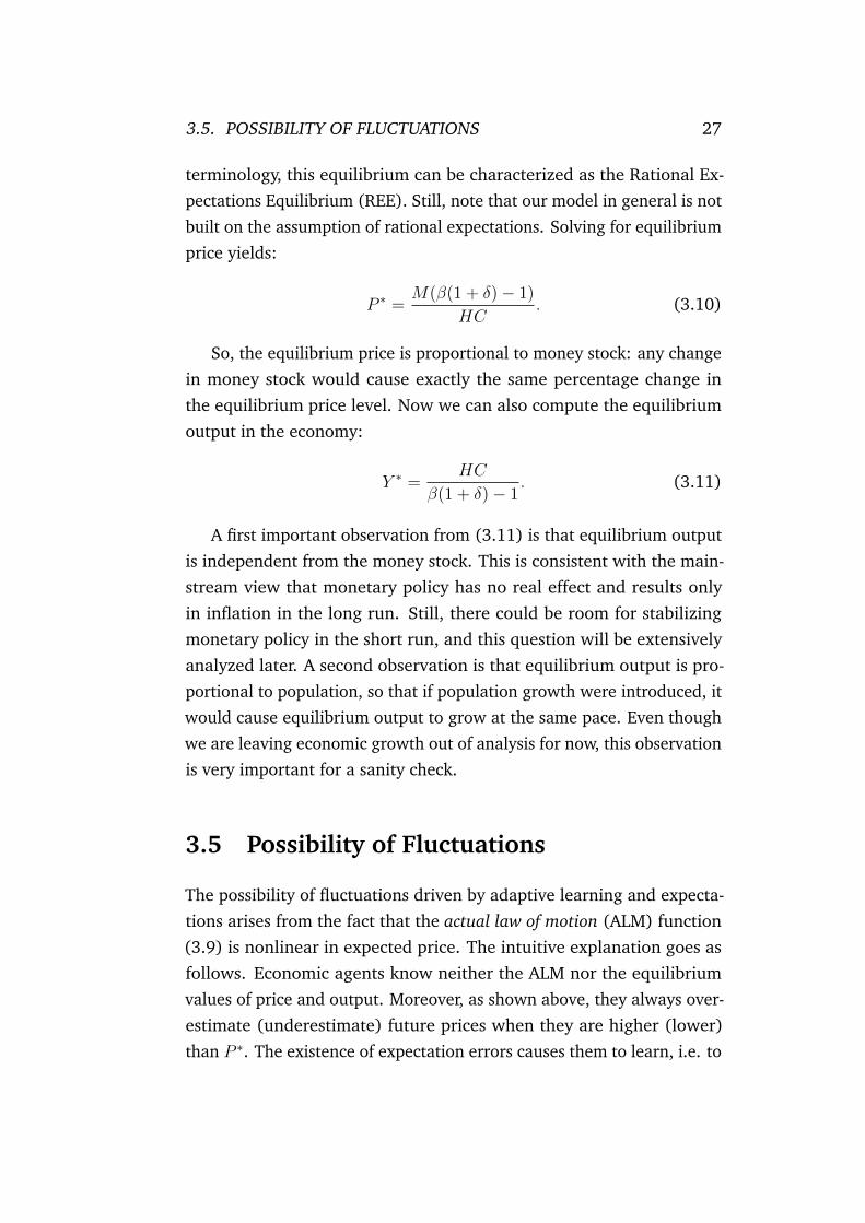
Figure 3.1: Timeline in Period t

price level.There is no nominal interest rate in the economy. Still, households

save part of their nominal income from various considerations, andeach period they are kind enough to borrow their savings for firms tomake investments. We assume that firms do not decide over capitaland passively invest what households save.1 This also ensures that theamount of money M is spent to purchase aggregate output. Since firms’cash inflow and outflow in each period equal exactly M , their retainedprofits are 0.

Figure 3.1 shows the timing of events in the model for each period t.First, each firm plans its production Qt and decides on how much laborLt it will employ given the available amount of capital (real savingsfrom previous period per firm: Kt =

HSt�1

NPt�1) and current wage (deter-

mined simultaneously). We assume that aggregate labor demand neverexceeds labor supply, so that firms can always hire the desired amountof labor. Next, price in period t is determined from the quantity equa-tion of money: Pt =

MYt

with Yt = NQt. Households and firms observePt and form their expectation of Pt+1.2 Having price expectations inplace, households decide on how to split their nominal income betweenconsumption and saving. Firms passively invest what households save,

1While this is obviously a strong assumption for any particular firm, it makes senseat the macro level, especially in a interest rate free environment.

2In this simple model we explicitly assume that households and firms have thesame expectations.

22 CHAPTER 3. MODEL

i.e. buy the good produced in the economy to use it as capital in thenext period.

Having described the timing, we proceed by expressing and solvingmathematically firms’ and households’ problems, assuming particularfunctional forms of the utility and production functions.

3.2 Firms and Economy Output

We assume that firms are price takers, i.e. they perceive themselves to betoo small to influence market price with output. Furthermore, firms areassumed to have Cobb-Douglas production function, with technology A

being constant over time.Therefore, each firm’s maximization problem at the beginning of

period t is:

max

Lt

n

P et AK

↵t L

�t � wtLt

o

. (3.2)

One important remark should be made regarding this maximizationproblem. In particular, note that firms are maximizing their nominalincome rather than the real one; moreover, expected price, which repre-sents also the expected aggregate price level, enters the same problemthat is solved to make decisions regarding real employment and output.Nonetheless, even though these properties may seem to contradict thewidespread view that an increase in the general price level should notstimulate firms to produce more, as their real profits do not change,the specification in (3.2) is not problematic in this sense. Think of afirm, that perceives itself to be too small to alter price or wage by itsdecisions, making plans for the next period. The only thing that this firmcan do is to maximize its nominal profit, as it automatically maximizesits real profit under given wage and expected price levels. To see that,divide (3.2) by P e

t to obtain the equivalent maximization problem inreal terms:

max

Lt

⇢

AK↵t L

�t �

wt

P et

Lt

�

,

3.2. FIRMS AND ECONOMY OUTPUT 23

where wtP et

is nothing else than expected real wage. The first ordercondition yields an expression for the firm’s decision Lt:

Lt =

✓

�P et AK

↵t

wt

◆

11��

. (3.3)

So, each firm would be willing to hire more when wage is lower,expected price is higher, and the firm has larger capital stock, whichincreases the marginal productivity of labor

Since the nominal constraint (3.1) should be satisfied, we can substi-tute (3.3) into (3.1) and solve for nominal wage:

wt =

✓

N

M �HSt�1

◆

1���

(�P et AK

↵t )

1� . (3.4)

Quite naturally, nominal wage positively depends on expected pricelevel and available capital. Combining (3.3) and (3.4) we can get anexpression for the actual amount of labor that each firm will hire:

Lt =

✓

M �HSt�1

N�P et AK

↵t

◆

1�

. (3.5)

Strikingly, after the elimination of nominal wage, hired amount labornow depends negatively on expected price and available capital! Thishas quite a straightforward explanation, however: when price expecta-tions and capital increase, the negative effect of wage on employmentobviously surpasses the expected revenue benefit. To clarify this pointeven further, note that obviously firms still make decisions using (3.3).Instead, equation (3.5) should be regarded as the macroeconomic result,coming from mechanisms that are not observable by any particular firm.

Substituting (3.5) into the production function, we obtain the actualproduction per firm:

Qt =M �HSt�1

N�P et

,

24 CHAPTER 3. MODEL

so that aggregate real output in the economy is:

Yt =M �HSt�1

�P et

. (3.6)

As in the case of employment, aggregate output negatively dependson expected price. Even though exaggerated due to the simplicity of themodel, this macroeconomic result is consistent with empirical evidencethat price in fact is countercyclical (Kydland and Prescott, 1982).

Another observation is that output in this simple model does notdepend on capital. The root of this result is the absence of interest rateand firms not deciding over investments. Treating available capital asconstant, firms choose the amount of labor that equates marginal laborproductivity with real wage. And since both marginal productivity andwage directly depend on capital, capital cancels out when computingactual output. This, however, is also consistent with the empiricalobservation that output has insignificant correlation with capital overthe business cycle (Kydland and Prescott, 1982).

Note that since St�1 is a function of past and expected prices asshown in the next section, price level is the only source of dynamics inthis model.

3.3 Households and Savings

We will ignore the labor supply decision for now3 and focus on theconsumption-savings decision. For simplicity, we assume that house-holds use logarithmic utility function to value current real consumptionand real savings expressed in expected purchasing power next period.As we show in section 3.6, this simplifying assumption does neitheraffect nor cause the main features and results of the model, whichare also valid under the most generic Hyperbolic Absolute Risk Aver-sion (HARA) utility function (algebra becomes cumbersome though).

3As we have already assumed, labor supply always exceeds demand. Since thewage is also determined through firms’ decisions and nominal constraint (3.1), weonly need labor supply to calculate the unemployment rate for illustrative purposes,and it does not have any effect on the dynamics of the economy in this model.

3.3. HOUSEHOLDS AND SAVINGS 25

Therefore, household’s maximization problem4 in period t becomes:

max

St

⇢

ln

✓

It � St

Pt

◆

+ � ln

✓

St

P et+1

+ C

◆�

. (3.7)

Here It and St are nominal income and savings of each householdin period t; 0 < � 1 is the weight of the savings part in the utility, sothat the weight on the consumption part is normalized to be 1; � canalso be seen as a subjective rate of time preference. C > 0 is a constantrequired to reduce marginal utility of savings; naturally, householdsexpect to earn some income next period, that would bring marginalutility of savings down, but for simplicity we avoid modeling incomeexpectations explicitly. Taking first order condition and solving for St,we obtain:

St =�

1 + �It �

C

1 + �P et+1. (3.8)

Nominal savings depend positively on current nominal income, butnegatively on expected price level next period. So, with simple loga-rithmic utility, only the substitution effect is at work, while the incomeeffect of expected relative price change is absent. Indeed, a householdsaves more as expected real interest rate5, i.e. Pt

P et+1

� 1, increases.6 Asshown in section 3.6, in case of HARA utility function, both effects areexplicitly present in the savings function, and the substitution effect

4It is further assumed that utility function is specified and being maximized atthe household level. While it is a rather unconventional approach, it may representreality better, since members of a household are expected to care about each otherand derive utility from making others feel better. For example, members that are ableto work, when deciding on their labor supply, will think not only about their owntrade-off between utility of higher consumption and disutility of effort, but also of thefact that they have to take care of other members of their households that are unableto work. Similarly, those who are staying at home obtain utility from other membersspending more time with them instead of working. Even though we have not proven itformally, we believe that one utility function may better represent this complicated setof synergies than the sum of individual utility functions.

5Remember that there is no contracted nominal interest rate in the model. Still,following Grandmont (1985), decrease in future price can be seen as real income, asif households were paid a real interest rate (which can, obviously, also be negative ifprice level increases).

6Some empirical evidence for this can be found, for example, in the overview byElmendorf (1996).

26 CHAPTER 3. MODEL

needs not necessarily dominate the income effect any more. However,as mentioned already, this does not affect the main findings of the paper.

3.4 Equilibrium Price Level and Output

In the model described above, expected price level determines output,which in turn determines actual price through the quantity equation ofmoney. Note that the nominal income of each household is predeter-mined to be It =

MH

. Substituting it in (3.8), putting the result in (3.6),and finally combining it with the quantity equation of money, we getthe actual law of motion for price:

Pt =M

Yt

=

�M

M �HSt�1P et

=

�M(1 + �)

M +HCP et

P et . (3.9)

Let us define equilibrium in the model as the state in which the pricelevel and output reach some fixed values P ⇤ and Y ⇤ and stay constantover time. Then it should also be the case that economic agents formcorrect expectations P e⇤

= P ⇤; if this was not the case, agents wouldadjust their expectations for the next period causing the price not beingconstant over time.

Call D(P et ) =

�M(1+�)M+HCP e

tthe price expectation multiplier, which itself

is a decreasing function of P et . It is straightforward to see that when

D is greater than 1, economic agents underpredict price; when D < 1,they overpredict the price; finally, when D = 1, economic agents formcorrect expectations of price.7

After substituting P ⇤ in (3.9) instead of all price variables, it isstraightforward to see that equilibrium price in the model would be thatsatisfying D(P ⇤

) = 1. Indeed, this condition guarantees that agents formcorrect expectations, and because of that, following a widely accepted

7The careful reader might have already noted that an economically less relevantcase of equilibrium is that with P e⇤ = P ⇤ = 0.

3.5. POSSIBILITY OF FLUCTUATIONS 27

terminology, this equilibrium can be characterized as the Rational Ex-pectations Equilibrium (REE). Still, note that our model in general is notbuilt on the assumption of rational expectations. Solving for equilibriumprice yields:

P ⇤=

M(�(1 + �)� 1)

HC. (3.10)

So, the equilibrium price is proportional to money stock: any changein money stock would cause exactly the same percentage change inthe equilibrium price level. Now we can also compute the equilibriumoutput in the economy:

Y ⇤=

HC

�(1 + �)� 1

. (3.11)

A first important observation from (3.11) is that equilibrium outputis independent from the money stock. This is consistent with the main-stream view that monetary policy has no real effect and results onlyin inflation in the long run. Still, there could be room for stabilizingmonetary policy in the short run, and this question will be extensivelyanalyzed later. A second observation is that equilibrium output is pro-portional to population, so that if population growth were introduced, itwould cause equilibrium output to grow at the same pace. Even thoughwe are leaving economic growth out of analysis for now, this observationis very important for a sanity check.

3.5 Possibility of Fluctuations

The possibility of fluctuations driven by adaptive learning and expecta-tions arises from the fact that the actual law of motion (ALM) function(3.9) is nonlinear in expected price. The intuitive explanation goes asfollows. Economic agents know neither the ALM nor the equilibriumvalues of price and output. Moreover, as shown above, they always over-estimate (underestimate) future prices when they are higher (lower)than P ⇤. The existence of expectation errors causes them to learn, i.e. to

28 CHAPTER 3. MODEL

update their tools used for forecasting to get more precise predictions.

If, for example, agents keep overpredicting price for a while, theywill eventually revise their forecasting tool to generate lower predictions,and vice versa. However, as they approach equilibrium from either side,not knowing what the equilibrium level is, they need not necessarily stopthere and may enter a zone where the sign of forecast errors reverses.After that, agents start to revise their expectation tool in the oppositedirection, and so on and so forth. Cycles that thereby arise remind thosein Pigou’s opening quotation: errors of optimism alternate with errorsof pessimism. Note that these cycles need not necessarily be decaying.Conducted simulations show that they may in fact diverge, dependingon the model fundamentals and learning rules, as shown in chapter 4.

It is also important to mention that it need not necessarily be thecase that agents do not know where the equilibrium is. It is sufficientthat they perceive themselves to be too small to affect market price andthat they are unable to cooperate to reach the equilibrium together. Ifthey realize that equilibrium is not going to happen, they simply wantto get the most precise forecast of future price to plan production andsavings.

3.6 Model with Hyperbolic Utility Function

In this section we show that the main results of the model preserve whenwe assume that households use the Hyperbolic Absolute Risk Aversion(HARA) utility function, and therefore do not rely on the simplifyingassumption of logarithmic utility. The uninterested reader may proceeddirectly to chapter 4.

Analyzing the model with HARA utility function is, in fact, just onestep short of a generic analysis, which is outside the scope of this thesisand left for future work. The HARA utility function presented in itsstandard form

U(W ) =

1� �

�

✓

↵W

1� �+ b

◆�

; ↵ > 0,↵W

1� �+ b > 0 (3.12)

3.6. MODEL WITH HYPERBOLIC UTILITY FUNCTION 29

nests almost all special cases used in the literature: linear utility when� = 1; quadratic utility when � = 2; constant absolute risk aversion(CARA) exponential utility function if b = 1 and � ! �1; and powerutility function if � < 1 and ↵ = 1 � �, which in turn nests constantrelative risk aversion (CRRA) utility function (b = 0) and logarithmicutility (� ! 0). 8

Preserving the assumptions from section 3.3 that households onlyoptimize over two periods and do not forecast their incomes, household’smaximization problem with HARA utility function becomes:

max

St

⇢

1� �

�

✓

↵(It � St)

(1� �)Pt

+ bc

◆�

+ �1� �

�

✓

↵St

(1� �)P et+1

+ bs

◆��

.

(3.13)

Analogously to the simple case with logarithmic utility, we claim thatit should be the case that bs > bc when � < 1, and bs < bc when � > 1,as, given all other parameters of utility items equal, we should accountfor the fact that households will receive income in period t+ 1, so thatmarginal utility from future consumption of current savings should beadjusted downwards. Taking the first order condition and solving forsavings, we obtain:

St =

�1

1�� It +(1��)↵

bc�1

1��Pt � bs

⇣

P et+1

Pt

⌘

�1��

P et+1

�

⇣

P et+1

Pt

⌘

�1��

+ �1

1��

. (3.14)

Let us have a close look at equation (3.14). It simplifies exactly to(3.8) when ↵ = 1 � �, � ! 0, and bc = 0. Next, we will eliminatethese specific parameter restrictions one by one and see what newcharacteristics each of them brings to the savings function.

First, if we make bc 6= 0, current price Pt will start having effect onsavings. So that savings now depend not only on expected inflation, butalso on observed one. If bs > bc > 0, then savings positively dependon current price level and negatively on expected inflation, i.e. the

8An overview of utility functions can be found in many textbooks on financialeconomics, e.g. in Cuthbertson and Nitzsche (2004)

30 CHAPTER 3. MODEL

substitution effect is at work. Indeed, in this case savings correlatepositively with expected real interest rate Pt

P et+1

� 1. If, on the other hand,bc < bs < 0, then only the income effect plays a role.

Secondly, eliminating the condition of � ! 0 leads to the savingsfunction becoming nonlinear in prices. Whether savings depend posi-tively or negatively on current and expected prices is now ambiguous.We postpone thorough analysis of this issue until we get to the ALM func-tion. Finally, easing ↵ = 1� � further adjusts the impact of prices in thenumerator of (3.14), even though it appears to be the least importanteffect.

As before, we obtain the actual law of motion of price by substituting(3.14) into (3.6), and combining the resulting equation for output withthe quantity equation of money:

Pt =

�M

✓

⇣

P et

Pt�1

⌘

�1��

+ �1

1��

◆

M⇣

P et

Pt�1

⌘

�1��

+H (1��)↵

bs

⇣

P et

Pt�1

⌘

�1��

P et � bc�

11��Pt�1

�P et , (3.15)

where the price expectation multiplier D(Pt�1, Pet ) can be defined as the

fraction in front of P et .

The derivation of equilibrium price and output is analogous to thatin section 3.4: for equilibrium price to be consistent with learning andexpectations formation, it should be the case that D(P ⇤, P ⇤

) = 1. Theobtained equations are:

P ⇤=

↵M⇣

� + ��1

1�� � 1

⌘

H(1� �)⇣

bs � bc�1

1��

⌘ , (3.16)

Y ⇤=

H(1� �)⇣

bs � bc�1

1��

⌘

↵⇣

� + ��1

1�� � 1

⌘ . (3.17)

Even though equations (3.16) and (3.17) are a bit more complicatedthan (3.10) and (3.11), they preserve the most important messagesof the latter. Firstly, equilibrium price is proportional to money stockM . And secondly, equilibrium output is proportional to population and

3.6. MODEL WITH HYPERBOLIC UTILITY FUNCTION 31

independent from the money stock, so that money stock is still neutralin the long run.

Having said that, it is now important to make several commentsabout the possibility of cycles in this setting. As discussed in section 3.5,cycles may emerge because of nonlinearity of the actual law of motion,particularly from the fact that agents always overestimate (underesti-mate) future prices when they are higher (lower) than P ⇤. So that, inPigou’s terms, errors of optimism will be forced to turn into errors ofpessimism, and vice versa.

Therefore, the necessary condition for fluctuations to emerge is thatthe price expectation multiplier D should be lower than 1 when pricesare higher than equilibrium level and greater than 1 when prices arebelow the equilibrium. In fact, this is also a sufficient condition forthe equilibrium to be stable, as if that was not the case, the economywould theoretically either shrink or diverge. Note, however, that thiscondition is not sufficient to observe cycles; whether fluctuations willactually emerge a great deal depends on how agents learn and formtheir expectations. We address this question in chapter 4.

However, what is not clear from the above paragraph is which pricesshould be compared with equilibrium level: expectation P e

t or previousrealization Pt�1? A somewhat inaccurate, but very simplifying andintuitive answer would be both. When what might be called the “generallevel of prices”, i.e. both realized and expected prices, is high, thenobviously D should be smaller than 1, and vice versa.

What complicates this simplistic view is that D(Pt�1, Pet ) is nonlinear

in both prices. It may well happen also that while realized price fromthe previous period is still above (below) P ⇤, expected price falls below(above) the equilibrium level. Moreover, the analysis is greatly compli-cated also by the fact that the ratio of prices matters: the sensitivityof D to P e

t , for example, will a great deal depend on Pt�1. A quicklook at the first derivatives D0

Pt�1and D0

P et

obtained in Mathematicaconfirms that further formal analysis would be an extremely challengingtask taking a lot of time and paper space, so we decided to leave itof out of the scope of this thesis. The rationale behind this decision

32 CHAPTER 3. MODEL

is best expressed by Willem Buiter’s words: “a privately and sociallycostly waste of time and other resources” (Buiter, 2009). Indeed, takinginto account the simplicity of the underlying assumptions of our model,there is no much value added, if any, from deriving very precise andcumbersome requirements for parameters in particular functional forms,except, maybe, demonstrating our strong mastery of algebra.

We proceed instead, just to give an example, with a fairly simpleand intuitive case, in which we can reduce the analysis of behavior ofthe function of two variables to a single-variable function. In particular,let us assume that agents have a very short memory and always expectthat currently observed price will be the same next period, i.e. P e

t =

Pt�1 = Pt. Then the “general level of prices” mentioned above becomesa single variable. However, we should bring the reader’s attention tothe fact that this simplification leads to the omission of the impact ofexpected real interest rate, or expected relative price change, on thesavings decision. Expected real interest rate under this assumption issimply always 0. Having said that, let us have a look at the resultingequation for the price expectation multiplier:

D(Pt) =

�M⇣

1 + �1

1��

⌘

M +H (1��)↵

⇣

bs � bc�1

1��

⌘

Pt

(3.18)

Since this function should be decreasing in Pt for equilibrium to bestable and to allow fluctuations to emerge theoretically,9 it should holdthat (1��)

↵

⇣

bs � bc�1

1��

⌘

> 0, which is equivalent to C > 0 in the simplecase with logarithmic utility. Given that ↵ > 0, it translates into therequirement that (i) bs > bc�

11�� when � < 1, and (ii) bs < bc�

11�� when

� > 1.

9In fact, as will be discussed in chapter 4, fluctuations will not emerge if expectationsare formed using an AR(1) model, which is exactly the case here.

Chapter 4

SIMULATION RESULTS

4.1 Economic Agents as Rational Econometri-

cians

In the previous chapter we have described the general setup of ourmodel, i.e. how the economy works and responds to actions of firmsand households, in particular to changes in their expectations. Now it istime to say something about how these expectations are formed.

One of our aims was to make agents behave more realistically thanin the DSGE models. On the other hand we did not want to engageinto incorporating various documented behavioral patterns in the modelsince (i) it is hard to distinguish which of them are the most importantfor economic fluctuations and (ii) there is also a risk of ending up witha very cumbersome model where it is not crystal clear how results areobtained. While acknowledging that the incorporation of findings frombehavioral economics could become a very powerful strand of researchand future work, we instead decided to maintain the assumption ofrational economic agents, but to make their rationality bounded.

Among the variety of possible ways to introduce bounded rational-ity, we found the approach described by Thomas Sargent in his bookBounded Rationality in Macroeconomics (1993) to be the most promising.Rather than knowing the whole underlying model of the economy, i.e.the actual law of motion, forming correct mathematical expectations of

33

34 CHAPTER 4. SIMULATION RESULTS

future outcomes which may not come true only because of exogenousshocks, and solving infinite horizon inter-temporal optimization prob-lems, as usually the inhabitants of DSGE models do, boundedly rationalagents instead are only left with the possibility to observe availableeconomic data, treat it rationally, produce forecasts over finite horizons,and, therefore, solve limited optimization problems. Based on this de-scription Sargent has developed a type of agents which he himself called‘rational econometricians’.

The idea is that agents should deal with available data as econome-tricians would: try to build and estimate as good an econometric modelas possible. While Sargent goes further in his book and discusses howe.g. AI could be used for this purpose, we stick to the simplest cases.Essentially, agents in our simulations estimate pre-specified econometricmodels using available data, make forecasts based on those models, andmake economic decisions as described in chapter 3. This approach isalso often referred to in the literature as adaptive learning, even thoughthe latter one is a broader concept.

It is important to notice that while Sargent and the bulk of literature1

on adaptive learning and expectations usually study models and attemptto find the conditions under which adaptive learning converges to ratio-nal expectations equilibrium (REE), we consider adaptive learning as asource of potential instability in our setting.

Let us now turn directly to the simulations.

4.2 Auto ARIMA in the Simple Logarithmic

Utility Case

In what follows we assume that economic agents try to model price asa time series without considering the possibility that other economicvariables may be useful in forecasting it. A short discussion is neededhere. On the one hand this assumption can be justified by the factthat, by design, all variables in the model are functions of realized and

1see e.g. Evans and Honkapohja (2001)

4.2. AUTO ARIMA IN THE SIMPLE LOGARITHMIC UTILITY CASE 35

expected price, and therefore there is no mechanical causality from e.g.unemployment rate to future price. On the other hand, if observedeconomic variables affect price expectations of economic agents, theyeffectively impact the actual price realizations. Moreover, observingthe co-movements in various economic variables may help firms andhouseholds to learn faster how the economy works, and make the systemmore stable. A larger number of variables can also cause confusion andbecome an additional source of instability. In short, the consequences ofrelaxing the above-mentioned assumption are ambiguous and dependon the particular learning tool that agents use.

We start with probably the most interesting and, at the same time,hardest to study formally learning tool: Auto ARIMA model. The ideais that every period agents select the best (according to some chosencriterion) ARIMA model based on the available price data and use it forforecasting. In this way we allow agents not only to update the coeffi-cients in their econometric model, but to change model specification aswell. Once again, this may either make the learning process faster andthe economy more stable, or become an additional source of instability.Also, switching models in favor of seemingly better ones may actuallynot be far from real life behavior.

To conduct the simulations we use R programming language. ForARIMA model selection the Bayesian information criterion (BIC) ischosen and auto.arima() function from package forecast is used. Eachperiod, after the price expectation is formed and aggregate output Y isdetermined, the latter is rounded to three digits after the decimal pointto prevent small and unobserved differences in the series to affect themodel selection. We take the logarithm of price data before feedingthem into auto.arima().2 The number of households and firms is 100

and 10 respectively, and money stock M equals 100. Technology A isunity and does not change over time. We assume constant return toscale so that ↵ + � = 1. Each simulation starts with the initial price

2There are two reasons for this: (i) taking the logarithm of prices prevents forecastsfrom being negative; (ii) if agents take the first difference of logged price data (whichauto.arima() can suggest), then they will be working with inflation rates, and it makeseconomic sense.

36 CHAPTER 4. SIMULATION RESULTS

expectation 1% above P ⇤, and then evolves as a purely deterministicprocess, without any kind of exogenous shocks. After the very firstperiod agents have only one observation of price, which is thereforetheir best guess for the second period, and which is exactly produced byauto.arima(). But as more price data becomes available, agents buildmore sophisticated ARIMA models.

A quite expectable question that may be asked by the careful readeris whether the fact that we start our simulations off the equilibrium canbe seen as an external shock. Our view is that there is absolutely noreason why agents should know and expect the equilibrium price levelat the “beginning of history.” If they are lucky enough to guess P ⇤ rightaway, then indeed no fluctuations will emerge. But this situation is nomore likely than them starting at 1.01 · P ⇤ or at any other level.

Figure 4.1a plots the output Y 3 from a simulation with labor pro-duction share � = 0.6 and subjective discount rate � = 0.7. All otherparameters are computed so that equilibrium output Y ⇤ equals 100 andP ⇤

= 1. The vertical grey lines indicate points where agents switchtheir models. The first and most important observation is that output in-deed fluctuates around its equilibrium level (horizontal line). Secondly,observed cycles are of varying length and amplitude: something thateconomists usually fail to achieve in standard RBC models.

The amplitude of output peaks roughly in the middle of the plot,when Y drops by around 4% of its equilibrium level. An interestingfact is that it is preceded by several drastic revisions of the models: inperiod 159 agents switch from ARMA(2,5) to AR(1); then, in period 160they switch to ARMA(2,2); and in period 163 they choose ARMA(3,1),which they maintain until the end of the simulation. This observationmay suggest an interesting hypothesis that major revisions of the agents’beliefs about how the economy functions may cause economic crises.

Figure 4.1b demonstrates that cycles can be also diverging. With� = 0.55 and � = 0.95, the amplitude of output fluctuations is constantlyincreasing. Note that the frequency of switching between model specifi-

3The plot of prices always mirrors that of output because of the quantity equationof money together with fixed M .

4.2. AUTO ARIMA IN THE SIMPLE LOGARITHMIC UTILITY CASE 37

(a) � = 0.6, � = 0.7

(b) � = 0.55, � = 0.95

Figure 4.1: Cycles in Simple Logarithmic Case

38 CHAPTER 4. SIMULATION RESULTS

cations is much higher here than on figure 4.1a. This supports the claimthat model switching may also be a serious source of instability.

It should be mentioned that in some cases of seemingly divergingsimulations, convergence towards equilibrium was observed in the longrun, while in other cases authors observed diverging oscillations withany simulation horizon.4 Formal analysis of this issue is needed, and inchapter 5 we will introduce a possible approach for future work on thisline.

4.3 Unemployment

It was assumed in the model setup that households’ labor supply does notmatter when employment, wage, production and prices are determined;firms are always able to hire the required amount of labor and wageis determined through labor demand and nominal constraint (3.1).However, if we wanted to show the behavior of unemployment in ourmodel, it would not be sufficient to just show the actual employment,as it reflects only firms decisions. It could well happen that households’labor supply is not constant and varies as economic conditions change.

To obtain labor supply in the economy, we modify the household’smaximization problem (3.7) to incorporate utility from leisure:5

max

St,lt

⇢

ln

✓

wtZlt + St�1 � St

Pt

◆

+ � ln

✓

St

P et+1

+ C

◆

+ µ ln (Z(1� lt))

�

.

(4.1)

Here Z is the size of one household, e.g. the number of people, ltis the fraction of employed individuals in each household,6 and µ is acoefficient representing the importance of leisure for households. In(4.1) households perceive that they can increase their nominal income

4Though it was not proved that these indeed diverge forever.5We continue with our assumption that utility being maximized at the household

level.6For example, it would be a normal situation when a household of Z = 7 people

consists of 4 elders, 2 working-age persons and one child. Then one would expectlt = 2/7 under normal economic conditions. lt can also be seen in a more traditionalway: as a fraction of the individual’s time allocated to work.

4.3. UNEMPLOYMENT 39

Figure 4.2: Umeployment Rate: µ = 2.65

by working more through wtZlt, even though in the end employment isdecided by firms and households only decide over savings as in (3.7).Taking first order conditions, solving for Zlt, and multiplying by thenumber of households H, we obtain total labor supply in the economy:

LSt =

H

1 + µ+ �

✓

Z(1 + �)� µSt�1 + CP e

t+1

wt

◆

. (4.2)

Labor supply (i) is proportional to the number of households; (ii)depends negatively on savings from the previous period, as householdshave less incentive to increase their nominal income; (iii) depends neg-atively on expected price next period, as it reflects the fact that house-holds will be able to buy less for the same amount of labor provided;(iv) depends positively on wage wt. Let us now turn to simulation.

Figure 4.2 plots the unemployment rate from the simulation with thesame parameters as on figure 4.1a in section 4.2. The black line showswhat the unemployment rate would be if households did not decide onhow much labor they would like to supply, i.e. LS is constant at its equi-

40 CHAPTER 4. SIMULATION RESULTS

librium level; while the red line shows the behavior of unemploymenttaking into account changes in labor supply. What we see on the plot,namely that the red line is more volatile than the black one, proves thehypothesis that changes in labor demand from firms tell only half ofthe story, and that the actual unemployment rate is more volatile, sincehouseholds are willing to work more during recessions and less duringeconomic booms.

It is worth mentioning also that the effect of labor supply may beunderstated in the above simulation due to the fact that we use loga-rithmic utility, which is usually associated with “myopish” behavior. Wesuspect that actual unemployment may be even more volatile in alter-native utility specifications, and studying unemployment under genericfunctional forms is worth effort in the future.

4.4 Multivariate Models

It was mentioned in section 4.2 that allowing agents to build multivariatemodels for predicting price has ambiguous consequences. In this sectionwe quickly sketch the preliminary results from simulations with agentsusing Vector Autoregressive (VAR) models.

In the following simulations we added wage as the additional vari-able. As estimating VAR models requires having some dataset already, inthe first half of the simulations data is generated with the auto.arima()function as in section 4.2, and then agents switch to VAR. We use thepackage vars in R. In every period, the function VARselect() is used tochoose the order of VAR model, and then the function VAR() is usedto estimate the value of the parameters of the model. As before, wetake the logarithm of price and wage data before feeding them into theVAR model to prevent the generation of negative forecasts in the case ofdiverging cycles. Figure 4.3 shows examples of obtained simulations.

Switching to VAR models turned out to be extremely destabilizingin our simulations. Even though there were cases when, following aquickly converging to equilibrium Auto ARIMA data generating process,the VAR part exhibited negligible fluctuations around the equilibrium,

4.4. MULTIVARIATE MODELS 41

(a) � = 0.55, � = 0.9

(b) � = 0.6, � = 0.95

Figure 4.3: Cycles with Agents Using VAR Models

42 CHAPTER 4. SIMULATION RESULTS

as shown on figure 4.3a, the overwhelming majority of simulationsresulted in rapidly diverging output once agents switch to VAR. Figure4.3b shows a typical simulation. The last few cycles have such a largeamplitude that all the previous fluctuations are hardly distinguishablefrom the equilibrium line; also, after period 300 the function VARselect()reported an error, as no suitable VAR model could be found any more.

Needless to say that the above result has to be treated with caution,however, as it is obtained with the simplest simulations imaginable. It isbased on the assumptions that agents know only reduced-form modeling,and are not able to develop “good” structural economic models.

4.5 Simulation with HARA Utility

It was shown in section 3.6 that the obtained results hold theoreticallywhen we switch from the simplifying assumption of logarithmic utilityto more generic utility functions, in particular Hyperbolic Absolute RiskAversion (HARA) utility.

Figure 4.4 shows that we can obtain both converging (figure 4.4a)and diverging (figure 4.4b) cycles when the parameters of the HARAutility function are selected so that it does not simplify to one of thepopular utility function types. As before, we assume that agents useAuto ARIMA. Constant return to scale is assumed, and the parameter bsis computed so that P ⇤

= 1 and Y ⇤= 100.

On both figure 4.4a and 4.4b we can see that the amplitude of fluctu-ations increases when the frequency of model switching increases. Thisis more evidence in support of the hypothesis that revisions by agents oftheir beliefs about how the economy works may trigger instability.

4.6 AR(2) and “False Equilibria”

All previous simulations were based on models with changing specifica-tions, and therefore are very hard to study formally. Here we consider asimpler case when agents have a pre-specified model and only update

4.6. AR(2) AND “FALSE EQUILIBRIA” 43

(a) � = 0.6, � = 0.85, bc = 0.03,� = �0.4, ↵ = 2

(b) � = 0.6, � = 0.8, bc = 0.2,� = �1, ↵ = 1

Figure 4.4: Cycles with Agents Having HARA Utility

44 CHAPTER 4. SIMULATION RESULTS

parameters over time. Two things motivate us for this exercise. Firstly,it is itself value-adding to show that cycles can emerge and proliferatein the economy even if agents do not switch model specification; modelswitching is then considered only as an additional source of instability.Secondly, sticking to one particular model specification opens the pos-sibility of formal analysis of how economy behaves in the long run, inparticular whether it diverges or not. More analysis of this question willfollow in chapter 5.

Our choice of the specification to study is the AR(2) model. It isfairly simple, yet yields business cycles and shows some unexpected andinteresting behavior. Also, it seems to be the case that for fluctuationsto emerge, one of the fundamental economic variables (most oftenoutput) should follow an autoregressive process at least of order 2.This is essentially achieved when agents use AR(2); all the simulationswith them using AR(1) resulted in price level and output smoothlyconverging to their equilibrium levels. It is very interesting and worthnoting that two of the most popular models of business cycles, theMultiplier-Accelerator model by P. Samuelson and the RBC model byKydland and Prescott, in different ways yield equations in which outputdepends on its values in the previous 2 periods, essentially following anAR(2) process.

Figure 4.5 shows the simulation with � = 0.7 and � = 0.45, in whichagents estimate the following AR(2) model:

Pt = �0 + �1Pt�1 + �2Pt�2, (4.3)

with the initial values of parameters �0 = 0.5, �1 = 1.6, and �2 = �1.These parameters are used in the first 5 periods, and after that, agentsstart to update them. Additionally, we introduce memory of length 300.This means that agents never use more than the 300 most recent priceobservations to estimate the parameters of their model.

Quite expectedly, output in the simulation exhibits cyclical fluctua-tions. However, as we can see, in the first 500 periods or so, it fluctuatesnot around its equilibrium level, but way below it, and only after cy-

4.6. AR(2) AND “FALSE EQUILIBRIA” 45

Figure 4.5: AR(2) Model with Memory and “False Equilibria”: � = 0.7,� = 0.45

cles almost die out, it starts to fluctuate once again, even with higheramplitude than before, this time around a value much closer to the equi-librium level. What happens here is that memory comes to play its role,and when instability at the beginning of the simulation is “forgotten”,agents suddenly realize that they are far off the equilibrium.

However, if memory was not introduced, this second wave of cycleswould never emerge, and output instead would follow the light-grayline, extremely slowly converging toward the equilibrium.7 The speedof convergence in this second case is so slow, that one can say thatthe economy is stuck in a “false equilibrium”.8 This notion very muchreminds of Keynes’s belief that the economy may end up being in adepressed state for a surprisingly long time, and therefore active gov-ernment intervention is needed to “cheer up” the animal spirits. In our

7This happens due to the fact that in this case the expectation multiplier D(P et ) is

only marginally different from unity.8Even though this is not an equilibrium technically speaking, and, of course, not an

exactly constant value over time.

46 CHAPTER 4. SIMULATION RESULTS

simulation the animal spirits were enlivened by short memory.

Chapter 5

EXPECTATIONAL STABILITY

In this chapter we present and attempt the application of some standardmethods for the analysis of the limiting behavior of stochastic systemswith adaptive learning.1 This is a highly technical part, the main purposeof which is to build a solid basis for future analysis; the uninterestedreader may proceed directly to chapter 6.

Instead, for further examination of the methods introduced in thischapter, the excited reader can refer to Sargent (1993), as well as toEvans and Honkapohja (2001, 2009).

5.1 Learning as a Recursive Algorithm

In the course of this chapter, unless otherwise specified, we only considerthe version of our model in which households have logarithmic utility.Moreover, we proceed by assuming that agents use an AR(2) model toforecast future prices based on past observations. This choice is justifiedby the fact that this model provides an effective trade-off betweensimplicity and usability.2 In other words, our assumption is that theperceived law of motion (PLM) is AR(2), so that agents form their

1Please note that in fact we are going to apply these methods to a deterministicsystem.

2On the one hand, the simplicity of an AR(1) model does not allow for the fluctua-tions to arise, making this case uninteresting from an economic perspective. On theother hand, auto ARIMA or VAR models have rather complex dynamics, making theirformal analysis an extremely challenging task.

47

48 CHAPTER 5. EXPECTATIONAL STABILITY

expectations fitting the following process:

Pt = �0 + �1Pt�1 + �2Pt�2 + "t,

where "t is an i.i.d. error term with zero mean. As an immediate result,we observe that

P et = �0 + �1Pt�1 + �2Pt�2.

Combining (3.9) with (5.1) we obtain the ALM as a function ofobserved prices:

Pt =�M(1 + �)(�0 + �1Pt�1 + �2Pt�2)

M +HC(�0 + �1Pt�1 + �2Pt�2). (5.1)

Given a set of starting values �0,�1,�2 and observations Pi withi = 1, 2, ..., t, it is possible to express the learning process (i.e. thedynamics of �0,�1,�2) over time by using the recursive least squares(RLS) algorithm. The result is the following system of two equations:

�t = �t�1 + t�1R

�1t pt�1(Pt � p

>t�1�t�1) (5.2)

Rt = Rt�1 + t�1(pt�1p

>t�1 �Rt�1) (5.3)

where pt := (1, Pt, Pt�1)>, �t := (�0t ,�1t ,�2t)

> and Rt is the momentmatrix for pt using observations Pi with i = 1, ..., t. From (5.1), notethat in fact Pt is a function of the previous period parameters �t�1

and observations pt�1; that is, Pt := f(�t�1,pt�1). Using this resultin (5.2), defining St�1 := Rt and moving (5.3) one period ahead, weobtain:

�t = �t�1 + t�1S

�1t�1pt�1(f(�t�1,pt�1)� p

>t�1�t�1) (5.4)

St = St�1 + t�1

✓

t

t+ 1

◆

(ptp>t � St�1). (5.5)

Formally, the system (5.4)-(5.5) is a recursive algorithm fully de-scribing agents’ learning dynamics at any time in the future, for giveninitial values. Our aim is now to investigate if and how it is possible to

5.2. THEORY OF STOCHASTIC APPROXIMATION 49

use this system to understand the asymptotic properties of our model.

5.2 Theory of Stochastic Approximation

Consider a (stochastic) recursive algorithm of the form

✓t = ✓t�1 + �tQ(t,✓t�1,xt(✓t�1)), (5.6)

where ✓t is the vector of parameter estimates, xt is the vector of obser-vations, and �t is a deterministic sequence of gains.

Following Evans and Honkapohja (2001), we know that it is possibleto study the limiting behavior of any recursive algorithm in the form of(5.6), by analyzing its associated ordinary differential equation (ODE).The latter is defined as

d✓

d⌧= h(✓(⌧)), (5.7)

where h(✓) is given by

h(✓) = limt!1

E [Q(t,✓, x̄(✓))] , (5.8)

with E[·] denoting the mathematical expectation operator and x̄(✓)

being the value of xt obtained by holding ✓t fixed at its limiting value,i.e. ✓t = ✓.

Most importantly, from stochastic approximation results,3 it is possi-ble to establish a direct correspondence between possible limiting pointsof the recursive algorithm, and locally stable equilibria of the ODE (5.7).

3cf. Marcet and Sargent (1989)

50 CHAPTER 5. EXPECTATIONAL STABILITY

5.3 An Application to Our Setting

Let us attempt an application of this result to our case. First of all, notethat the system (5.4)-(5.5) is indeed in the form of (5.6) with

✓t = vec(�t St)

xt = (1, Pt, Pt�1, Pt�2)>

�t = t�1.

Therefore, we can use (5.4)-(5.5) to retrieve the explicit form ofQ(·), so to study its properties. For simplicity we split the function intotwo components as follows:

Q�(t,✓, x̄) = S

�1p̄(f(�, p̄)� p̄

>�) (5.9)

QS(t,✓, x̄) =

✓

t

t+ 1

◆

(p̄p̄

> � S). (5.10)

We can now use (5.9) and (5.10) to find the ODEs associated to thesystem (5.4) - (5.5):

h�(�) = limt!1

E

S

�1p̄

✓

�M(1 + �)(p̄>�)

M +HC(p̄

>�)

� p̄

>�

◆�

(5.11)

hS(S) = limt!1

E

t

t+ 1

(p̄p̄

> � S)

�

. (5.12)

First, it is important to observe that in our case everything inside theexpectation operator is deterministic. That is, there is no stochastic partthat might prevent us from taking expectations of each single componentseparately.

Second, let us call p̂ := (1, ˆP , ˆP )

> the mathematical expectation ofp̄. Note that either p̂ = (1, P ⇤, P ⇤

)

> or p̂ = (1, 0, 0)> because for anyother value of p̂ a fixed � would not be sustainable, since the learningprocess would cause it to change. Therefore, it is not rational to expectany value of p̂ other than those two.

Furthermore, defining W := E[p̄p̄

>] = p̂p̂

>, it is easy to see that

5.3. AN APPLICATION TO OUR SETTING 51

(5.12) becomes

hS(S) = W � S,

implying the first condition for equilibria of the ODE to be W = S.Replacing this result in (5.11) and solving, we obtain

h�(�) = �

✓

�M(1 + �)

M +HC(p̂

>�)

� 1

◆

. (5.13)

This is the core ODE defining possible limiting points of our recursivealgorithm (5.4)-(5.5).

Even though formally we should speak of equilibria of the ODE interms of �, it is more illustrative to present them in terms of P e. In fact,we can see that (5.13) has two equilibria in terms of P e. The first onecorresponds to the solution of

�M(1 + �)

M +HC(p̂

>�)

� 1 = 0

and that is P e= P ⇤, while the second one corresponds to � = 0 and

implies P e= 0.4 Interestingly enough, we will see that the second equi-

librium can be disregarded since it is locally unstable for any meaningfulchoice of parameters.

However, before moving to the determination of local stability, it isinteresting to note that the analysis of (5.13) is indeed greatly compli-cated by the nonlinearity of the ALM.5 Intuitively, this seems to be afurther confirmation of the importance of this factor in our model forthe provision of adequate dynamics for the generation of cycles. Thatis, non-linearities seem to play an important role in the functioning ofthe economy, suggesting that heavy reliance on linear approximationsmight cause a loss of important features of the economic system.

To investigate the stability of these fixed points, we derive the Jaco-

4Note that indeed these equilibria correspond to the two points that were identifiedin chapter 3. Furthermore, please note also that technically there is an infinite numberof equilibria identifiable in terms of �.

5cf. Evans and Honkapohja (2001) for cases with linear ALM.

52 CHAPTER 5. EXPECTATIONAL STABILITY

bian matrix of the function on the right-hand side of (5.13). DefiningA :=

�M(1+�)M+HC(p̂>�) and B :=

�HCM+HC(p̂>�) , it is possible to express the

Jacobian as

J =

0

B

B

@

(A� 1) + (AB)�0 (AB ˆP )�0 (AB ˆP )�0

(AB)�1 (A� 1) + (AB ˆP )�1 (AB ˆP )�1

(AB)�2 (AB ˆP )�2 (A� 1) + (AB ˆP )�2

1

C

C

A

,

where either ˆP = P ⇤ or ˆP = 0.

From fundamental results on the stability of ODEs, we know that ifall the eigenvalues of J evaluated at a fixed point have negative realparts, then that fixed point is locally asymptotically stable. Instead, ifat least one eigenvalue of J evaluated at a fixed point has positive realpart, then that fixed point is locally asymptotically unstable.

Finally, let us define K := J � �I, where � is a 1⇥ 3 vector and I isthe 3 ⇥ 3 identity matrix. To obtain the eigenvalues of J , we need tosolve det(K) = 0.

5.4 Convergence for the Case of � = 0

We are now going to consider local stability of the equilibrium of (5.13)characterized by � = 0. As already mentioned, this case can also beexpressed as P e

= P = 0.

Other than a simple example, this analysis is relevant in that a credi-ble economic model can afford neither to allow its agents to expect azero price nor certainly to permit the economy to actually reach thatlevel; even more so considering that in the latter case production wouldbe infinite. That is to say, even if in reality it might be a desirable situa-tion, we certainly do not want to model an economy where productioncan be infinite and everything can be free of charge.

First of all, let us note that in this case the matrix K is greatlysimplified by the fact that �0 = �1 = �2 = 0. Let us call K0 the matrix

5.5. NOTES ON CONVERGENCE FOR PE= P ⇤ > 0 53

resulting from such a simplification of K. Then,

K0 =

0

B

B

@

[�(1 + �)� 1]� � 0 0

0 [�(1 + �)� 1]� � 0

0 0 [�(1 + �)� 1]� �

1

C

C

A

,

implying that J has only one eigenvalue with multiplicity 3, i.e. �1 =�2 = �3 = �(1 + �)� 1. Thus, the condition for P e

= P = 0 to be locallyasymptotically stable becomes:

�(1 + �)� 1 < 0

� <1

1 + �.

However, by looking at (3.10) it is easy to note that for this conditionto be verified, the equilibrium price P ⇤ has to be negative.6 This, inturn, implies that for any positive equilibrium price P ⇤, the economywill never converge to the fixed point with � = 0 and P e

= P = 0 unlessit starts from it, which is clearly never the case in our setting. That is,for any reasonable set of parameters, our economy will never convergeto an economically meaningless equilibrium solution.

One more conclusion that can be drawn from this result is thatp̂ = (1, P ⇤, P ⇤

)

> for all the relevant cases. In fact, if P ⇤ > 0 and theeconomy does not start with � = 0, then we have just proved that itwill never converge to a point with P e

= P = 0. Thus, one should notmathematically expect it to do so.

5.5 Notes on Convergence for Pe = P ⇤ > 0

Even though the equilibrium of (5.13) characterized by P e= P ⇤ > 0

is more cumbersome to treat analytically, we can at least simplify thematrix K in view of our latter result. In fact, by noting that we can use(3.10) to substitute for P ⇤, and that in this case:

1) p̂ = (1, P ⇤, P ⇤)

>,6This is the case because M , H and C must all be positive to make economic sense.

54 CHAPTER 5. EXPECTATIONAL STABILITY

2) P e= P ⇤,

3) P ⇤= �0 + �1P

⇤+ �2P

⇤,

one can obtain the following ‘simplified’ version of K:

KP ⇤=

0

B

B

B

B

B

B

B

@

(a� 1)(1� �1 � �2)� � (a�1)2

ba(1� �1 � �2)

(a�1)2

ba(1� �1 � �2)

(ba)�1 (a� 1)�1 � � (a� 1)�1

(ba)�2 (a� 1)�2 (a� 1)�2 � �

1

C

C

C

C

C

C

C

A

,

with a :=

1�(1+�) and b = �HC

M.7

Having obtained KP ⇤, with some tedious algebra it is possible toshow that in this context the eigenvalues of the Jacobian matrix aregiven by the solutions of

�3 � �2(a� 1) + �⇣

(a� 1)�1�2(a� 1� ba)⌘

�⇣

(a� 1)

2(1� �1 � �2)�1�2(a� 1� ba)

⌘

= 0.(5.14)

It is certainly possible to solve analytically (5.14) by using a standardcubic formula. However, in view of the complexity of the solution, itwould be hard to make economic sense out of it.

A smarter approach would be to consider the case in which P ⇤= 1,

exactly as we imposed in all simulations in chapter 4. Note that sinceP ⇤

=

a�1ba

= 1, equation (5.14) simplifies to

�3 � �2(a� 1) = 0, (5.15)

and it is now easy to see that the solutions of (5.15) are

�1 = (a� 1)

�2 = 0.

7Please note that this implies P ⇤ = a�1ba .

5.5. NOTES ON CONVERGENCE FOR PE= P ⇤ > 0 55

However, while �1 < 0 is indeed verified for all cases with P ⇤ > 0,8

the presence of a null eigenvalue complicates the analysis in the sensethat it would require us to consider at least terms of second-order (i.e.the Hessian matrix) of (5.13) to formally identify the exact conditionsfor stability, and therefore convergence.

In line with the exemplary and introductory role of this chapter wedecide not to follow that path. However, an interesting and powerfulapproach that could be taken in future research is the application ofnumerical methods in the attempt of shedding light on this kind ofmathematical problems.

8Obviously this is the case because we assume, as it should be done, that M , H andC are all positive.

Chapter 6

STABILIZING MONETARYPOLICY

A central banker comes into the caffe and orders a cake. Thewaiter asks:– Would you like it cut into 6 or 12 pieces?The central banker replies:– 6, please, I do not feel like eating 12.

In this chapter we will analyze the possibility of stabilizing monetarypolicy in our simple model. As already noted, this model is characterizedby long-run money neutrality; i.e. any permanent increase in M wouldlead to a proportional increase in the equilibrium price P ⇤ (see equations(3.10) and (3.16)), leaving the equilibrium level of output Y ⇤ unaffected(see equations (3.11) and (3.17)). Still, a possibility exists that shifts inthe money stock may affect output in the short-run, making stabilizingmonetary policy possible and the above joke not funny any more.

6.1 Monetary Policy with Simple Logarithmic

Utility

Let us first investigate whether monetary policy is effective in the settingwhere households have a simple logarithmic utility function. To conduct

56

6.1. MONETARY POLICY WITH SIMPLE LOGARITHMIC UTILITY 57

this formal analysis, we change the previously constant money stock M

into Mt. The actual law of motion of price from (3.9) becomes:

Pt =�Mt(1 + �)

Mt +HCP et

P et , (6.1)

while the ALM for output is:

Yt =Mt

�(1 + �)P et

+

HC

�(1 + �). (6.2)

Looking at equation (6.2) as a function of time, it is straightforwardto note that it contains a fixed part and a variable part, with the latterdepending positively on the money stock Mt and negatively on priceexpectation P e

t .

The immediate observation from equation (6.2) is that monetarypolicy does not have any real effect even in the short run if economicagents know exactly the upcoming change in the money stock and adjusttheir initial price expectation by the same proportion; i.e. if they knowthat the money stock is going to increase by x% next period and theyconsequently increase their price expectation by exactly x%. It is easyto see from (6.1) that in this case actual price will also increase by x%.Even without any formal proof, it is intuitive to see therefore that suchbehavior of agents is consistent with learning experience: if actual pricealways responds to change in the money stock exactly as agents expectit to, they have no reasons to change their beliefs.

In light of this result, there are only two cases in which short-termstabilizing monetary policy can actually work in this model: (i) themonetary policy is in part unexpected, i.e. agents do not know exactlywhat money supply will be in the next period; (ii) agents believe thatchanges in the money stock, for some reason, do not imply exactly thesame change in prices (at least in the short run). While the first casebelongs to a rather political discussion on transparency of central banksand not much on it can be said here, we will have a closer look at thesecond one.

Let us investigate what happens if agents believe that a x% change

58 CHAPTER 6. STABILIZING MONETARY POLICY

in the money stock does not cause a proportional shift in price level,resulting instead in a percentage change of price equal to · x%, > 0.This would imply that the derivative of price expectation with respectto the money stock equals: @P e

t@Mt

= P et

Mt. Furthermore, it is easy to verify

that the derivative of actual price with respect to the money stock is:

@Pt

@Mt

= �(1 + �)M2

t@P e

t@Mt

+HCP e2t

(M +HCP et )

2,

which, after substituting @P et

@Mt, becomes:

@Pt

@Mt

= �(1 + �) Mt +HCP e

t

(M +HCP et )

2P et . (6.3)

For the so called -belief to be sustainable within an adaptive learn-ing environment, it should be the case that actual price responds tochanges in the money stock also with the rate , implying @Pt

@Mt= Pt

Mt=

�(1 + �) M+HCP e

tP et . However, It is straightforward to see that if < 1

( > 1) the ‘responsiveness’ of actual price is greater (smaller) than .Therefore, any value of other than unity is not sustainable from thelearning perspective, because at some point agents would realize thattheir belief is not coming true and update it in the correct direction. Thequestion is, however, whether they will converge to = 1 or end upfluctuating around this value.

If they do converge, then the ultimate conclusion is that monetarypolicy may initially have short-term real effects, but it will become inef-fective in the longer perspective when (and if!) learning is completed.

On the other hand, as long as agents keep changing their beliefsregarding over time, stabilizing monetary policy will remain possible.However, as will be changing, the same will do the responsiveness ofprice and output to monetary shocks according to (6.3). Therefore, evenassuming that a central bank knows exactly how the economy functions,it would also need to know the market sentiment, i.e. what economicagents expect from monetary policy, to operate effectively. Same shifts inthe money stock may have very different effects depending on economic

6.2. STABILIZING POLICY IN A GENERAL SETTING 59

situation.

6.2 Stabilizing Policy in a General Setting

The conclusions made in the previous section change even further infavor of the effectiveness of monetary policy if we consider the actuallaw of motion of output when agents use a more generic HARA utilityfunction:

Yt =

Mt

⇣

P et

Pt�1

⌘

�1��

+H (1��)↵

bs

⇣

P et

Pt�1

⌘

�1��

P et � bc�

11��Pt�1

�

�P et

✓

⇣

P et

Pt�1

⌘

�1��

+ �1

1��

◆ (6.4)

Indeed, now even if agents knew exactly the upcoming shift in moneystock and adjusted their expectations proportionally, these adjustmentssimply would not cancel out as they did in (6.2). Therefore, monetaryinterventions will always have real effects on the economy!

However, central bankers should refrain from celebrating too early.In fact, only if they knew precisely how the economy works, knew theexact values of all the coefficients in the model, and, moreover, knewvery well agents’ price expectations and how these expectations reactto news about monetary policy; in other words, if they were some kindof economic gods, then indeed they would be able to conduct a veryeffective stabilizing monetary policy.

There is no reason to believe, however, that central bankers knowsignificantly much more about the economy than economists at researchdepartments of large private companies and banks. After all, theyusually go to the same schools and study the same economic theoriesand econometric methods. The hard truth is also that private institutionsusually offer higher salaries. To sum up, it is highly doubtful that centralbanks can assess accurately the consequences of their own actions, andtherefore they should not abuse the power they have.

Having said that, we should cheer up our disillusioned centralbankers and tell them that monetary policy is not going to be thrown

60 CHAPTER 6. STABILIZING MONETARY POLICY

away. As someone has said, it is better to do something imperfectly thando nothing perfectly. If the economy is obviously falling into a recession,or is already in a crisis, monetary intervention will have a real (andhopefully positive) effect, and therefore might be used. Not to mentionthe situation of “false equilibrium” shown in section 4.6, in which casemonetary policy is one of the instruments able to move the economyback on track.

Chapter 7

DISCUSSION ANDCONCLUDING REMARKS

In this concluding chapter we would like to quickly systemize our find-ings and point out the most interesting and relevant directions for futurework. The contributions of this thesis largely belong to two major fieldsof economics: business cycle theory and effectiveness of stabilizing mon-etary policy. We will shortly describe our findings in a consecutive order,discussing possible improvements and extensions on the way.

I.

With a simple, growth-less macroeconomic model, we show theo-retically that business cycles can emerge endogenously in the economywhen agents do not have perfect foresight, learn adaptively to form ex-pectations, and solve limited inter-temporal optimization models. Thispossibility largely arises from the nonlinearity of the actual law of mo-tion of price, in particular from the fact that agents always overpredict(underpredict) future prices when they are higher (lower) than equi-librium level. Even though the main version of the model is based onhouseholds having simple logarithmic utility function, we also show thatour results hold when a more generic Hyperbolic Absolute Risk Aversionutility function is chosen. Interestingly enough, Money stock is neutralin the long run in either case.

61

62 CHAPTER 7. DISCUSSION AND CONCLUDING REMARKS

We see three ways in which our model should be developed further.Firstly, we believe that the most important next step would be to aban-don the use of particular functional forms for the utility and productionfunctions, and move to the analysis of a fully generic setting. A greaterdegree of generality is preferable in that it would potentially allow thederivation of necessary and sufficient conditions on the shape1 of theutility and production functions for the emergence and proliferation ofcycles. This mighty task however, requires more time and maturity ofthe research, and will appear in future publications.

Secondly, the model can be extended to become more realistic. In-troducing growth, making agents forecast and optimize over longerhorizons, incorporating additional important economic variables suchas contracted interest rate, could all greatly enhance the usability of themodel, if done in a simple and elegant way.

The third thing that could be done is deriving the same results ina completely alternative setting. Developing a “more standard, moreIS-LM’y, with-Philips-Curve’y” model2 could bring this line of researchto a qualitatively new level, perhaps even making its message accessibleto a more general public.

II.

We conduct simulations in models with agents having both simplelogarithmic and HARA utility functions. Following Sargent (1993), weassume agents to be “rational econometricians” using various econo-metric adaptive learning tools: Auto ARIMA, VAR and AR(2) models.In all simulations, output and other economic variables indeed displaycyclical fluctuations around their equilibrium levels, without the intro-duction of any kind of exogenous shocks to productivity or any otherfundamental parameters of the economy, in contrast to RBC models.To our knowledge this thesis is the first attempt to formally introduce

1As opposed to deriving conditions on parameters, that often becomes cumbersomewhen parametrization rises.

2A very valuable advice given by Prof. George Akerlof at the ISEO Summer School2013, for which we are extremely grateful to him.

63

adaptive learning and expectation errors as an autonomous source ofendogenous business cycles.

Both converging and diverging cycles may be obtained in simula-tions with Auto ARIMA models, while the VAR learning tool leads todiverging fluctuations in the majority of cases, suggesting that makingagents consider several variables increases instability, at least in oursetting. It is also observed that higher frequency of model switching isusually accompanied with increasing amplitude of cycles, suggestingthe hypothesis that economic crises may happen when agents makedrastic revisions of their beliefs about how the economy works. Onlyconverging cycles could be obtained with AR(2), however in this casethe economy may get trapped in a so called “false equilibrium”, withoutput way below or above the true equilibrium level. Even though thisis not formally an equilibrium, the convergence towards the true oneis so slow that exogenous shocks may be needed to move the economyback on track. This result is in line with the Keynesian view that theeconomy may remain in a depressed state for quite a long period oftime, and active government intervention may be required to speed upthe recovery.

However, in conducted simulations, the behavior of the economy hasproved very sensitive to the specified learning tools, initial conditions,and parameters of the model. Therefore, more work should be donein order to achieve a better understanding of how the dynamics of theeconomy depend on all of these preconditions. Once again, genericanalysis would be of great help here.

A major extension would be to make agents build structural economicmodels instead of using simple reduced-form modeling. This wouldrequire developing AI and a “rational theorist” type of agents. Thisdirection for future research was also first outlined in Sargent (1993).A promising idea for economic historians would be to check if majoreconomic perturbations can indeed be explained by significant revisionsin economic theory.

We believe there to be a major step between running simulationsand calibrating a model in order to reproduce real-world economic

64 CHAPTER 7. DISCUSSION AND CONCLUDING REMARKS

dynamics. In fact, not only the possibility of calibration would allow abetter evaluation of the empirical fit of our model, but it could also openthe possibility of using it for economic forecasting and policy analysis.This, of course, can be done only when the above mentioned extensionsand improvements are already accomplished.

III.

Within the developed framework we analyze whether active mone-tary policy (i.e. changes in money stock) can be used for stabilizationpurposes. It turns out that in the simple case, when agents have loga-rithmic utility function, shifts in money supply can have real effects onthe economy only if they are unexpected by agents, or if future priceexpectations are not adjusted exactly proportionally to the announcedmonetary interventions. We also show that the second case is not sus-tainable within the adaptive learning environment, so that monetarypolicy may become ineffective in the long run when, and if, learning iscomplete.

We prove, however, that monetary interventions always have realeffects in the short run in the setting with a more generic HARA utilityfunction. Still, it is highly questionable whether the central bank is ableto accurately assess the consequences of its own actions, as that wouldrequire it knowing precisely the actual law of motion of the economy,current market’s expectations, and agents’ reaction to news about theupcoming monetary interventions, which, moreover, can change overtime. In fact, there are no reasons to believe that central bankers aresystematically smarter than economists at private institutions.

Nevertheless, monetary policy might be an effective instrument tomove the economy back on track when it is entering a recession or stuckin a crisis. Our point is rather that central banks should not abuse thepower they have and overdo what is required from them.

Furthermore, one might be worried whether monetary intervention,while initially having a positive effect on output, would not cause moreeconomic instability and higher amplitude of business cycles later, whenagents start to revise their forecasting models in view of an increased

65

difference between their expectations and actual outcomes. Simulationsof the consequences of shifts in money supply in a longer perspectivesmight become an important practical application of our model in thefuture. It would be an interesting exercise also to simulate a settingin which the central bank is trying to learn the actual law of motionand conduct stabilizing monetary policy, and compare the results withsimulations where the central bank is absent.

Bibliography

Andolfatto, D. (1996). Business cycles and labor-market search. Ameri-can Economic Review, 86(1):112–32.

Barro, R. J. (1980). A capital market in an equilibrium business cyclemodel. Econometrica, 48(6):1393–1417.

Beaudry, P. and Portier, F. (2004). An exploration into pigou’s theory ofcycles. Journal of Monetary Economics, 51(6):1183–1216.

Benhabib, J. and Farmer, R. E. (1999). Indeterminacy and sunspots inmacroeconomics. In Taylor, J. B. and Woodford, M., editors, Handbookof Macroeconomics, Handbook of Macroeconomics, chapter 6, pages387–448. Elsevier.

Black, F. (1982). General equilibrium and business cycles. NationalBureau of Economic Research, NBER Working Paper No. 950.

Brunner, K., Cukierman, A., and Meltzer, A. H. (1983). Money andeconomic activity, inventories and business cycles. Journal of MonetaryEconomics, 11(3):281–319.

Buiter, W. (2009). The unfortunate uselessness of most ‘state of theart’ academic monetary economics. Financial TImes. Willem Buier’sMaverecon.

Cellarier, L. L. (2008). Least squares learning and business cycles.Journal of Economic Behavior and Organization, 68(3-4):553–564.

Cogley, T. and Nason, J. M. (1995). Output dynamics in real-business-cycle models. American Economic Review, 85(3):492–511.

66

BIBLIOGRAPHY 67

Cuthbertson, K. and Nitzsche, D. (2004). Quantitative Financial Eco-nomics: Stocks, Bonds and Foreign Exchange. Wiley, 2nd edition.

Dosi, G., Fagiolo, G., and Andrea, R. (2006). An evolutionary model ofendogenous business cycles. Computational Economics, 27(1):3–34.

Elmendorf, D. W. (1996). The effect of interest-rate changes on house-hold saving and consumption: a survey. Board of Governors of theFederal Reserve System (U.S.), Finance and Economics DiscussionSeries: 96-27.

Eusepi, S. and Preston, B. (2011). Expectations, learning, and businesscycle fluctuations. American Economic Review, 101(6):2844–2872.

Evans, G. W. and Honkapohja, S. (2001). Learning and Expectations inMacroeconomics. Frontiers of Economic Research. Princeton UniversityPress.

Evans, G. W. and Honkapohja, S. (2009). Learning and macroeconomics.Annual Review of Economics, 1(5):421–451.

Farmer, R. E. A. and Guo, J.-T. (1994). Real business cycles and theanimal spirits hypothesis. Journal of Economic Theory, 63(1):42–72.

Grandmont, J.-M. (1985). On endogenous competitive business cycles.Econometrica, 53(5):995–1045.

Hansen, G. D. (1985). Indivisible labor and the business cycle. Journalof Monetary Economics, 16(3):309–327.

Hayek, F. (1931). Prices and Production. 2nd ed. Routledge, London.

Hicks, J. R. (1950). A Contribution to the Theory of the Trade Cycle.Clarendon Press, Oxford.

Howitt, P. and McAfee, R. P. (1992). Animal spirits. American EconomicReview, 82(3):493–507.

Huang, K. X., Liu, Z., and Zha, T. (2009). Learning, adaptive expecta-tions and technology shocks. Economic Journal, 119(536):377–405.

68 BIBLIOGRAPHY

Jaimovich, N. and Rebelo, S. (2007). Behavioral theories of the businesscycle. Journal of the European Economic Association, 5(2-3):361–368.

Juglar, C. (1862). Des Crises commerciales et leur retour periodique enFrance, en Angleterre, et aux Etats-Unis. Guillaunim, Paris.

Keynes, J. M. (1936). The General Theory of Employment, Interest andMoney. Macmillan, London.

Kydland, F. E. and Prescott, E. . (1982). Time to build and aggregatefluctuations. Econometrica, 50(6):1345–1370.

Lengnick, M. (2011). Agent-based macroeconomics - a baseline model.Economics Working Papers, Christian-Albrechts-University of Kiel,Department of Economics, No. 2011-04.

Long, J. B. and Plosser, C. L. (1983). Real business cycles. Journal ofPolitical Economy, 91(1):39–69.

Lucas, R. J. (1972). Expectations and the neutrality of money. Journalof Economic Theory, 4(2):103–124.

Lucas, R. J. (1973). Some international evidence on output-inflationtradeoffs. American Economic Review, 63(3):326–334.

Lucas, R. J. (1975). An equilibrium model of the business cycle. Journalof Political Economy, 83(5):1113–1144.

Lucas, R. J. (1976). Econometric policy evaluation: A critique. Carnegie-Rochester Conference Series on Public Policy, 1(1):19–46.

Malthus, T. R. (1836). Principles of Political Economy. 2rd ed. WilliamPickering, London.

Marcet, A. and Sargent, T. J. (1989). Convergence of least squares learn-ing mechanisms in self-referential linear stochastic models. Journal ofEconomic Theory, 48(2):337–368.

Merz, M. (1995). Search in the labor market and the real business cycle.Journal of Monetary Economics, 36(2):269–300.

BIBLIOGRAPHY 69

Milani, F. (2011). Expectation shocks and learning as drivers of thebusiness cycle. Economic Journal, 121(552):379–401.

Mises, L. (1912). The Theory of Money and Credit. (H.E. Batson, trans.)Liberty Fund, Indianapolis, 1981.

Mitchell, W. C. (1927). Business Cycles: The Problem and Its Setting.National Bureau of Economic Research.

Mortensen, D. T. and Pissarides, C. A. (1994). Job creation and jobdestruction in the theory of unemployment. Review of EconomicStudies, 61(3):397–415.

Muth, J. F. (1961). Rational expectations and the theory of price move-ments. Econometrica, 29(6):315–335.

Paul, O. (2003). The us business cycle: an agent-based model of het-erogenous firms operating under uncertainty. Society for Computa-tional Economics, Computing in Economics and Finance 2003, N.90.

Pigou, A. C. (1927). Industrial Fluctuations. Macmillan, London.

Prescott, E. C. (1986). Theory ahead of business cycle measurement.Carnegie-Rochester Conference Series on Public Policy.

Ricardo, D. (1817). On the Principles of Political Economy and Taxation.3rd ed. John Murray, London, 1821.

Samuelson, P. A. (1939). Interactions between the multiplier analy-sis and the principle of acceleration. The Review of Economics andStatistics, 25(Autumn):11–44.

Sargent, T. J. (1993). Bounded Rationality in Macroeconomics. OxfordUniversity Press, Oxford.

Sargent, T. J. and Wallace, N. (1975). ‘rational’ expectations, the optimalmonetary instrument, and the optimal money supply rule. Journal ofPolitical Economy, 85(1):163–190.

70 BIBLIOGRAPHY

Say, J.-B. (1803). A Treatise on Political Economy or the Production,Distribution and Consumption of Wealth. A.M. Kelley Publishers, NewYork, 1971.

Schumpeter, J. A. (1912). Theorie der wirtschaftlichen Entwicklung.Dunker & Humblot, Leipzig.

Schumpeter, J. A. (1939). Business Cycles: A Theoretical, Historical, andStatistical Analysis of the Capitalist Process. McGraw-Hill, New Yorkand London.

Sismondi, J. C. L. (1819). New Principles of Political Economy: Of Wealthand Its Relation to Population. (R. Hyse, trans. and ed.) TransactionPublishers, New Brunswick, 1991.

Wen, Y. (2001). Understanding self-fulfilling rational expectations equi-libria in real business cycle models. Journal of Economic Dynamics andControl, 25(8):1221–1240.

Williams, N. (2003). Adaptive learning and business cycles. Manuscript,Princeton University.

Woodford, M. (1990). Learning to believe in sunspots. Econometrica,58(2):277–307.