Embed Size (px)
Citation preview
Computational Economics (2005)
DOI: 10.1007/s10614-005-9014-2 C© Springer 2005
An Evolutionary Model of Endogenous
Business Cycles
GIOVANNI DOSI,1 GIORGIO FAGIOLO2 and ANDREA ROVENTINI3
1Sant’Anna School of Advanced Studies, Laboratory of Economics and Management, PiazzaMartiri della Liberta, I-56127 Pisa, Italy; E-mail: [email protected] of Verona, Italy and Sant’Anna School of Advanced Studies, Pisa, Italy3Sant’Anna School of Advanced Studies, Pisa, Italy and University of Modena and Reggio Emilia,Italy
Abstract. In this paper, we present an evolutionary model of industry dynamics yielding endogenous
business cycles with ‘Keynesian’ features. The model describes an economy composed of firms
and consumers/workers. Firms belong to two industries. The first one performs R&D and produces
heterogeneous machine tools. Firms in the second industry invest in new machines and produce a
homogenous consumption good. Consumers sell their labor and fully consume their income. In line
with the empirical literature on investment patterns, we assume that the investment decisions by firms
are lumpy and constrained by their financial structures. Moreover, drawing from behavioral theories
of the firm, we assume boundedly rational expectation formation. Simulation results show that the
model is able to deliver self-sustaining patterns of growth characterized by the presence of endogenous
business cycles. The model can also replicate the most important stylized facts concerning micro- and
macro-economic dynamics. Indeed, we find that investment is more volatile than GDP; consumption is
less volatile than GDP; investment, consumption and change in stocks are procyclical and coincident
variables; employment is procyclical; unemployment rate is anticyclical; firm size distributions are
skewed but depart from log-normality; firm growth distributions are tent-shaped.
Key words: evolutionary dynamics, agent-based computational economics, animal spirits, lumpy
investment, output fluctuations, endogenous business cycles
JEL Classifications: C15, C22, C49, E17, E22, E32.
1. Introduction
The existence of widespread and persistent fluctuations which permanently affectthe overall economic activity is an inherent feature of all modern economies. How-ever, despite the huge number of competing models providing a rationale for ex-pansions and recessions, we still lack a generally accepted explanation for businessfluctuations. Indeed, it still holds largely true that a good deal of research has beenmainly concerned with ‘theoretical possibilities, rather than with explanations ofwhat actually happens,’ with ‘little regard for how the pieces fit each other and thereal world’ (Zarnowitz, 1985, p. 570). Ultimately, the theory of business cycle ap-pears to be ‘long of both good and poor questions and short of persuasive answers’(Zarnowitz, 1997, p. 2).
G. DOSI, G. FAGIOLO AND A. ROVENTINI
A primary example of such a mismatching might be found in the ways eco-nomic theory deals with the stylized facts concerning microeconomic investmentdynamics and business cycle properties. A robust macroeconomic empirical lit-erature has indeed shown that, at the aggregate level, investment is consider-ably more volatile than output and consumption less volatile. Moreover, fluctu-ations of both output and its main components (i.e. investment, consumption andchanges in inventories) tend to be synchronized. Finally, at the microeconomic level,firms’ investments appear to be lumpy and strongly affected by firms’ financialstructures.
Needless to say, one does indeed find huge streams of work on business cyclesmostly belonging either to the Real Business Cycle (RBC) perspective or to theNew-Keynesian (NK) one. This is not the place to undertake a review of the litera-ture (on RBC, cf. King and Rebelo (1999) and Stadler (1994); on NK theories, seeMankiw and Romer (1991) and Greenwald and Stiglitz (1993)). Let us just mentionhere the basic mechanisms generating cycles in the two perspectives. Real-businesscycles are ultimately driven by exogenous and unpredictable technological shocks,which generate fluctuating dynamics in a stochastic general-equilibrium world,grounded upon a fully-rational, forward-looking representative agent. Conversely,the basic story of NK models finds the roots of economic fluctuations in product-,labor- and financial-market imperfections (including in primis informational asym-metries). At the same time, these models do allow for some heterogeneity, at leastin the functional roles of the agents (the economy is in fact populated by financialinvestors, firms, consumers, etc.), even if under the disguise of ‘representative’,fully rational types.
Certainly, one finds very hard to believe the existence of macroscopic tech-nological shocks (including negative ones) necessary for the RBC story to hold.1
And, conversely, while the informational setting of NK models is much more rea-sonable, we still feel uneasy about the almost exclusive emphasis upon monetaryand price shocks as drivers of the fluctuations, while neglecting all technologicalfactors.
Moreover, in our view, a major weakness – shared to different degrees by bothstreams of literature – is the persistent clash between the microeconomics thatone finds in the models and the regularities in microeconomic behaviors that oneempirically observes. So, for example, notwithstanding the proliferation of modelsseparately trying to account for micro and macro stylized facts, almost no attemptshave been made in the literature to explain the properties of business cycles onthe basis of multiple individual entities embodying the observed microeconomicregularities about firms’ investment and pricing behaviors.
In this paper, we try to bridge such a gap by proposing a model whereboth output and investment dynamics are grounded upon lumpy investmentdecisions undertaken by boundedly-rational firms constrained by their finan-cial structure, but, at the same time, always able to discover new productiontechnologies.
AN EVOLUTIONARY MODEL OF ENDOGENOUS BUSINESS CYCLES
First, we fully take on board the critique to the ‘representative agent fallacies’(Kirman, 1989, 1992) and describe an economy with heterogeneous agents thatinteract in explicitly modeled markets.
Second, well in line with Keynesian intuitions, we assume pervasive marketuncertainty, so that investment and pricing decisions are taken on the grounds ofboundedly-rational rules, most often involving adaptive expectations. In turn, suchdecisions bear permanent aggregate demand effects.
Conversely, third, the ‘Schumpeterian’ feature of the model regards the persistentarrival of technological innovations, entailing multiple endogenously generatedmicro-shocks on productivity.
The model depicts an economy composed by firms (operating in two vertically-linked industries), consumers/workers and a (unmodeled) non-market sector. Firmsin the ‘upstream’ industry perform R&D and produce technologically heteroge-neous machines. The latter are used in the ‘downstream’ industry to produce aconsumption good bought by workers with their wages and by recipients of in-comes in the non-market sector.
The work belongs to the evolutionary, ‘agent-based computational economics’(ACE), family.2 In each period t , firms and workers carry out their production,investment, and consumption decisions on the basis of routinized behavioral rulesand (adaptive) expectations. The dynamics of microeconomic variables (i.e. indi-vidual production, investment, consumption, etc.) thus induces the macroeconomicdynamics for aggregate variables (e.g. aggregate output, investment, consumption,etc.), whose statistical properties are then studied and compared with empiricallyobserved ones.
Simulation results show that the model is able to deliver self-sustaining growthpatterns characterized by endogenous business cycles. Moreover, we show that themodel is able to replicate those business cycle stylized facts (e.g. volatility, auto-and cross-correlation patterns) actually observed. Finally, the micro-structure of thesimulated economy is quite in tune with the evidence on e.g. persistent heterogeneityin firm efficiencies, size and growth rate distributions.
The rest of the paper is organized as follows. Section 2 provides a short overviewof micro and macro empirical evidence. In Section 3, we discuss the antecedents andtheoretical roots of our model, which we formally present in Section 4. Qualitativeand quantitative results of simulation exercises are discussed in Section 5. Section 6concludes.
2. Aggregate Fluctuations and Micro Regularities: Some Evidence
To repeat, a good check of the robustness of any model claiming to be able to‘explain’ business cycles ought to rest in its ability to account together for morethan one macroeconomic ‘stylized fact’ and ought to do it in ways which arecoherent with the observed microeconomics of business decisions and innovationpatterns. Let us thus consider the most relevant empirical regularities.
G. DOSI, G. FAGIOLO AND A. ROVENTINI
2.1. MACRO STYLIZED FACTS
A key issue in the empirical business cycle literature concerns the properties ofaggregate output and of its main components (i.e. investment, consumption andinventories).
All available statistical evidence suggests that recurrent fluctuations have char-acterized the whole history of industrial economies. This applies also to the periodafter WWII, when aggregate output and its main components have experienced animpressive long term growth in the U.S. as well as in other developed countries.Even then, however, time-series display growth together with persistent ‘cyclical’turbulences. This can be seen also if the dynamics of output and its components isanalyzed at the business cycle frequencies: there, the series display a typical ‘rollercoaster’ shape, implying the repeated interchange of expansions and recessionswhich are part of the very definition of the business cycle.3
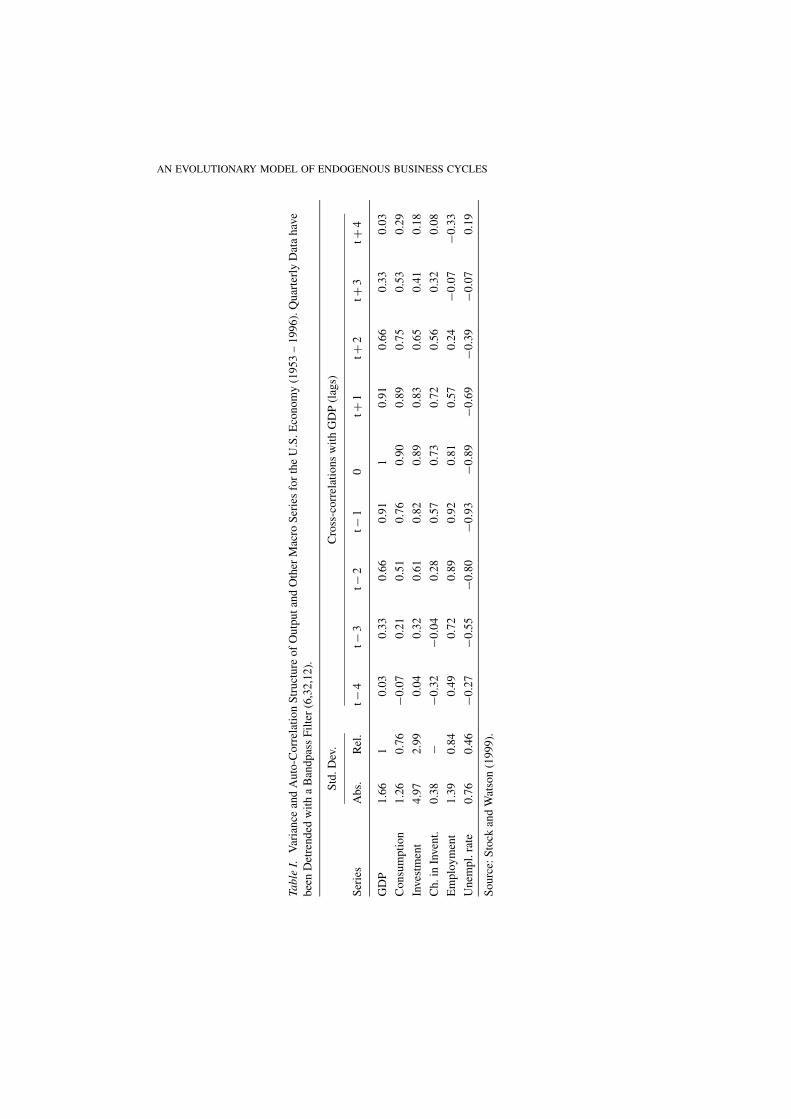
Thus, the evidence pre- and post-WWII – which we summarize in Table I-corroborates the seminal observations dating back to Kuznets (1930) and Burnsand Mitchell (1946), suggesting the following stylized facts:4
SF1 Investment is considerably more volatile than output.SF2 Consumption is less volatile that output.SF3 Investment, consumption and change in inventories tend to be procyclical and
coincident variables.5
SF4 Aggregate employment and unemployment rate tend to be lagging variables.The former is procyclical, whereas the latter is anticyclical.
2.2. MICRO STYLIZED FACTS
Over the last couple of decades, the empirical literature on industrial dynamics andtechnological change has singled out an impressive number of robust statisticalregularities concerning the microeconomic properties of firm behavioral patterns.Let us begin here with a telegraphical account of those stylized facts pertaining tofirms’ investment decisions.
SF5 Investment is lumpy.SF6 Investment is influenced by firms’ financial structure.
Consider first SF5. As shown by the important work of Doms and Dunne (1998)based on U.S. plant level data, lumpiness is an intrinsic feature of firm investmentdecisions: in a given year, 51.9% of all plants increase their capital stock by lessthan 2.5%, while the 11% of them raise it by more than 20%. Moreover, within-plant investment patterns show that plants typically invest in every single year, butthey concentrate half of their total investment in just three years out of the sixteenunder analysis.
Moreover, the microeconomic lumpiness of investment does not appear tobe completely filtered away at the macroeconomic level. Aggregate investment
AN EVOLUTIONARY MODEL OF ENDOGENOUS BUSINESS CYCLES
Tabl
eI.
Var
ian
cean
dA
uto
-Co
rrel
atio
nS
tru
ctu
reo
fO
utp
ut
and
Oth
erM
acro
Ser
ies
for
the
U.S
.E
con
om
y(1
95
3–
19
96
).Q
uar
terl
yD
ata
hav
e
bee
nD
etre
nd
edw
ith
aB
and
pas
sF
ilte
r(6
,32
,12
).
Std
.D
ev.
Cro
ss-c
orr
elat
ion
sw
ith
GD
P(l
ags)
Ser
ies
Ab
s.R
el.
t−4
t−3
t−2
t−1
0t+
1t+
2t+
3t+
4
GD
P1
.66
10
.03
0.3
30
.66
0.9
11
0.9
10
.66
0.3
30
.03
Co
nsu
mp
tio
n1
.26
0.7
6−0
.07
0.2
10
.51
0.7
60
.90
0.8
90
.75
0.5
30
.29
Inves
tmen
t4
.97
2.9
90
.04
0.3
20
.61
0.8
20
.89
0.8
30
.65
0.4
10
.18
Ch
.in
Inven
t.0
.38
−−0
.32
−0.0
40
.28
0.5
70
.73
0.7
20
.56
0.3
20
.08
Em
plo
ym
ent
1.3
90
.84
0.4
90
.72
0.8
90
.92
0.8
10
.57
0.2
4−0
.07
−0.3
3
Un
emp
l.ra
te0
.76
0.4
6−0
.27
−0.5
5−0
.80
−0.9
3−0
.89
−0.6
9−0
.39
−0.0
70
.19
So
urc
e:S
tock
and
Wat
son
(19
99
).
G. DOSI, G. FAGIOLO AND A. ROVENTINI
fluctuations are indeed influenced by the number of plants incurring huge investmentepisodes: the correlation between aggregate investment and the number of plantsexperiencing their maximum investment share is 0.59.
As far SF6 is concerned, the evidence is even more impressive. Since the influ-ential work of Fazzari, Hubbard, and Petersen (1988), a huge stream of empiricalliterature6 has been providing evidence against the Modigliani and Miller (1958)theorem. Indeed, if capital markets are imperfect (e.g. because of information asym-metries), the financial structure of the firm is likely to affect its investment decisions.First, the cost of external financing is typically higher than that of internal financ-ing: the larger information costs born by each firm, the higher the gap between thecost of internal and external financing. Second, information asymmetries may leadlenders to ration credit to the riskiest firms. These propositions are supported bythe evidence provided by the so-called ‘financial constraints’ literature: ceteribusparibus, firm investment is significantly correlated with cash flows (a proxy for networth variations) and the correlation magnitude is higher for those firms that suffermore from information asymmetries plaguing capital market (e.g. young and smallfirms).7
Regarding the drivers of growth, a growing number of contributions has robustlyhighlighted the central role of technological learning, innovation and diffusioncarried out by business firms (see Dosi, Freeman, and Fabiani (1994) for a criticaloverview; more detailed discussions are in Rosenberg (1982, 1994), Freeman (1982)and Dosi (1988)).
The idea that aggregate growth can be traced back to business history findsquantitative roots in a series of robust stylized facts put forth by the literature onthe microeconomics of innovation. In a synthesis:
SF7 Firms are the main locus where technological accumulation takes place.Technological learning - as well as its directions and rates – is carried outby firms in ways which are strongly shaped by: (a) firm-specific abilities;(b) richness of perceived unexploited opportunities. As a consequence,technological learning and accumulation tends to be mostly local: tech-nical advances typically occur in a neighborhood of currently-masteredtechnologies. This cumulative learning pattern is ‘punctuated’ by major,low-probability advances which generate jumps in the technological space(i.e. changes in the technological paradigms).
SF8 Innovations take time to diffuse. Technological diffusion is slowed down byinformation asymmetries and, even more important, by the fact that firmsrequire time to learn how to master new technologies and develop new skills.
SF9 Most innovations are industry-specific. Therefore, the overall pattern ofbusiness fluctuations cannot be fully explained by economy-wide innovativeshocks.
In turn, the foregoing regularities concerning innovation and technological diffu-sion map onto the intersectoral patterns of realized performances and productivities.
AN EVOLUTIONARY MODEL OF ENDOGENOUS BUSINESS CYCLES
Extensive studies on longitudinal micro-level data sets – ranging from the seminalwork of Nelson (1981) to the survey in Bartelsman and Doms (2000) – confirm thatproductivity dynamics is characterized by a few robust regularities, namely:
SF10 Productivity dispersion among firms is considerably large.SF11 Inter-firm productivity differentials are quite persistent over time.
Moreover, heterogeneity concerns firm size distributions, both among firmsbelonging to the same industrial sector and across different industrial sectors (see,among a vast literature, and Bottazzi and Secchi (2003b,a)).
SF12 Firm size distributions tend to be considerably right skewed, with upper-tailsmade of few large firms. These patterns vary significantly across differentsectors.
As discussed at more length in e.g. Bottazzi, Cefis, and Dosi (2002), the forego-ing regularity obviously supports the view that real-world markets strongly departfrom perfect competition. Moreover, a growing evidence highlights microeconomicprocesses of growth entailing some underlying correlation structure and lumpiness.More precisely:
SF13 Firm growth-rate distributions are not Gaussian and can be well proxied byfat-tailed, tent-shaped densities.
According to SF13, firm growth patterns tend to display relatively frequent‘big’ – negative or positive – growth events.
In the model presented below, we take explicitly on board micro-regularitiespertaining to firm investment and innovating behaviors (SF5 – 9) in the way wedesign the agents populating our economy, with the aim of building a model that,at the same time, is able to replicate and explain the stylized facts concerning thebusiness cycle (SF1 – 4) on the basis of micro-dynamics patterns which replicatethe statistical regularities displayed by the evolution of firm productivity, size andgrowth over time (SF10 – 13).
3. Theoretical Roots and Antecedents
We have already mentioned that the model which follows belongs to the evolu-tionary family. The seminal reference here is Nelson and Winter (1982). The workshows, among other things, the straightforward possibility of generating patterns ofmacroeconomic growth akin those observed in reality, on the grounds of a microe-conomic structure made of heterogeneous agents that continuously try to innovateand imitate new techniques of production. There, however, any ‘Keynesian’ de-mand propagation effect is censored by construction, and so it is in many othermodels of evolutionary inspiration.8
The first attempts to explore the properties of evolutionary models with‘Keynesian’ demand propagation effects can be found in Chiaromonte and Dosi
G. DOSI, G. FAGIOLO AND A. ROVENTINI
(1993) and in the simpler but multi-economy framework studied in Dosi, Fabiani,Aversi, and Meacci (1994). In the former, one describes a two-sector economy withmachine-embodied innovations, imperfect competition and two fundamental feed-backs running from investment to wages to aggregate demand (the ‘multiplier’),and, the other way round, from aggregate demand to investment (the ‘accelerator’).
The present model refines upon this early templates and, for the first time,analyzes the fine statistical properties of the ensuing dynamics. Moreover, the modelbelow tries to explicitly capture in its behavioral assumptions some of the microregularities mentioned above.
Consider, for instance, investment lumpiness (cf. SF5). It is well-known that thelatter can be in principle interpreted as the outcome of some optimizing behavior ofa perfectly-rational firm. This is indeed what the so-called (S,s) investment modelsdo.9 In that framework, firms face the problem of choosing the level of capitalmaximizing their flow of profits. If their desired capital is larger than the actualone, firms want to invest as long as they are able to recover capital adjustmentcosts. However, if the latter present some non-convexities, firms will invest up tosome optimal target level (S) only if their capital imbalance is lower than a givenoptimal trigger threshold (s). Therefore, investment lumpiness straightforwardlyderives from non-convexity of adjustment costs.
Notwithstanding the awareness that investment lumpiness may have significantconsequences at the macro level, almost no attempts have been made to embed theobserved microeconomic investment behavior into a business cycle model.10 Morespecifically, a surprisingly little attention has been paid so far to the interpretationof the stylized facts concerning the business cycle discussed above on the basis ofthe microeconomic evidence on firm investment behavior (cf. SF5 and SF6).
In this paper, we take a preliminary step in this direction. In our model, invest-ment can be either employed to increase the capital stock or to replace existingcapital goods. Consumption-good firms plan their expansion investment accordingto a (S,s) pattern. However, we depart from the standard lumpy investment litera-ture in modeling firms as boundedly-rational agents. In particular, we assume thatfirms employ routinized behavioral investment rules instead of fully-rational, profit-maximizing behaviors cum non-convex adjustment costs (on routinized behaviors,see – within an enormous literature – Nelson and Winter (1982), Dosi (1988), Cyertand March (1989) and, much earlier, Katona and Morgan (1952)).
We interpret the target and trigger levels of an (S,s)-type of investment behaviorin terms of a routinized investment rule, rather than as the outcome of some opti-mization procedure. Indeed, firms operating in ‘evolutionary environments’ (Dosi,Marengo, and Fagiolo, 2005) typically face strong uncertainty and cannot attachany probability measure to future outcomes (more on that in Dosi and Egidi (1991)).Hence, the adoption of a (S,s) rule fulfills the goals of a prudent, risk-averse, firmwhich is not able to fully anticipate its future level of demand and forms its ex-pectations in an adaptive fashion. Firms will then decide to expand their stock ofcapital only if they expect a significant demand growth. As a result, they will invest
AN EVOLUTIONARY MODEL OF ENDOGENOUS BUSINESS CYCLES
to reach their target level of capital only if the fulfillment of their expected demandrequires a capital stock at least equal to their trigger level.
Similarly to what happens for expansion investment, firms employ routinizedbehaviors to decide their replacement investment.11 In particular, we introduceheterogenous capital goods and we assume that firms implement their replacementpolicy through a payback-period routine. In this way, technical change and capitalgood prices enter in the replacement decisions of consumption-good firms.
Finally, the financial structure of the firm does affect in our model its investmentpolicies (cf. SF6). Indeed, the presence of financial constraints implies that firmspay a premium if they rely on external sources of funds (i.e. credit). Therefore, thefinancial structure of firms might not be neutral: firms may turn to external creditwhen their stock of liquid assets is not enough to fully finance their investmentplans.
4. The Model
We model an economy populated by F firms and L workers/consumers. Firmsare split in two industries: there are F1 consumption-good firms (labeled by j inwhat follows) and F2 machine-tool firms (labeled by i). Of course, F = F1 +F2. Consumption-good firms invest in machine-tools and produce a homogeneousproduct for consumers. Machine-tool firms produce heterogenous capital goods andperform R&D. Workers inelastically sell labor to firms in both sectors and fullyconsume the income they receive. Investment choices of consumption-good firmsdetermine the level of income, consumption and employment in the economy.
In the next subsection, we shall firstly describe in a telegraphic way the dynamicsof events in a representative time-period. Next, we shall provide a more detailedaccount of each event separately.
4.1. THE DYNAMICS OF MICROECONOMIC DECISIONS
In any discrete time period t = 1, 2, . . . , the timeline of events runs as follows:12
1. Consumption-good firms take their production and investment decisions. Ac-cording to their expected demand, firms fix their desired production and, if nec-essary, invest to expand their capital stock. A payback period rule is employedto set replacement investment. Credit-rationed firms finance their investment,first with their stock of liquid assets, and next, if necessary, with debt.
2. Capital-good market opens. Market shares and their changes depend on the‘competitiveness’ of each machine-producing firm.
3. Consumption-good market opens. Consumption-good production takes place.Unemployment rates and monetary wage emerge as the collective outcome ofmicro-decisions. The size of the consumption-good demand depends on thenumber of workers employed by firms. Consumption-good firms facing imper-fectly informed consumers receive a fraction of the total demand as a functionof their price competitiveness.
4. Exit, technical change and entry. Firms facing negative net liquid assets and/or a
G. DOSI, G. FAGIOLO AND A. ROVENTINI
non-positive market-share exit and they are replaced by new firms. Capital-goodfirms stochastically search for new machines.
Finally, total consumption, investment, change in inventories, and total productare obtained by aggregating individual time-t quantities.
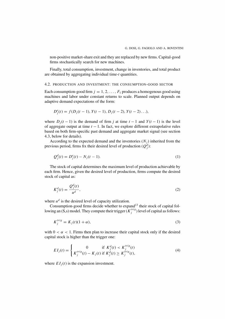
4.2. PRODUCTION AND INVESTMENT: THE CONSUMPTION-GOOD SECTOR
Each consumption-good firm j = 1, 2, . . . , F1 produces a homogenous good usingmachines and labor under constant returns to scale. Planned output depends onadaptive demand expectations of the form:
Dej (t) = f (D j (t − 1), Y (t − 1), D j (t − 2), Y (t − 2) . . .),
where D j (t − 1) is the demand of firm j at time t − 1 and Y (t − 1) is the levelof aggregate output at time t − 1. In fact, we explore different extrapolative rulesbased on both firm-specific past demand and aggregate market signal (see section4.3, below for details).
According to the expected demand and the inventories (N j ) inherited from theprevious period, firms fix their desired level of production (Qd
j ):
Qdj (t) = De
j (t) − N j (t − 1). (1)
The stock of capital determines the maximum level of production achievable byeach firm. Hence, given the desired level of production, firms compute the desiredstock of capital as:
K dj (t) = Qd
j (t)
ud, (2)
where ud is the desired level of capacity utilization.Consumption-good firms decide whether to expand13 their stock of capital fol-
lowing an (S,s) model. They compute their trigger (K trigj ) level of capital as follows:
K trigj = K j (t)(1 + α), (3)
with 0 < α < 1. Firms then plan to increase their capital stock only if the desiredcapital stock is higher than the trigger one:
E I j (t) ={
0 if K dj (t) < K trig
j (t)
K trigj (t) − K j (t) if K d
j (t) ≥ K trigj (t),
(4)
where E I j (t) is the expansion investment.
AN EVOLUTIONARY MODEL OF ENDOGENOUS BUSINESS CYCLES
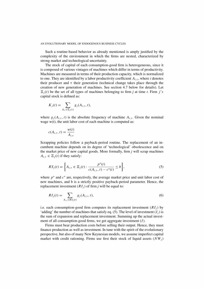
Such a routine-based behavior as already mentioned is amply justified by thecomplexity of the environment in which the firms are nested, characterized bystrong market and technological uncertainty.
The stock of capital of each consumption-good firm is heterogeneous, since itis composed of various vintages of machines which differ in terms of productivity.Machines are measured in terms of their production capacity, which is normalizedto one. They are identified by a labor productivity coefficient Ai,τ , where i denotestheir producer and τ their generation (technical change takes place through thecreation of new generation of machines. See section 4.7 below for details). Let� j (t) be the set of all types of machines belonging to firm j at time t. Firm j’scapital stock is defined as:
K j (t) =∑
Aiτ ∈� j (τ )
g j (Ai,τ , t),
where g j (Ai,τ , t) is the absolute frequency of machine Ai,τ . Given the nominalwage w(t), the unit labor cost of each machine is computed as:
c(Ai,τ , t) = w(t)
Ai,τ
Scrapping policies follow a payback-period routine. The replacement of an in-cumbent machine depends on its degree of ‘technological’ obsolescence and onthe market price of new capital goods. More formally, firm j will scrap machinesAi,τ ∈ � j (t) if they satisfy:
RSj (t) ={
Ai,τ ∈ � j (t) :p∗(t)
c(Ai,τ , t) − c∗(t)≤ b
}, (5)
where p∗ and c∗ are, respectively, the average market price and unit labor cost ofnew machines, and b is a strictly positive payback-period parameter. Hence, thereplacement investment (RI j ) of firm j will be equal to:
RI j (t) =∑
Ai,τ ∈RSj (t)
g j (Ai,τ , t), (6)
i.e. each consumption-good firm computes its replacement investment (RI j ) by‘adding’ the number of machines that satisfy eq. (5). The level of investment (I j ) isthe sum of expansion and replacement investment. Summing up the actual invest-ment of all consumption-good firms, we get aggregate investment (I ).
Firms must bear production costs before selling their output. Hence, they mustfinance production as well as investment. In tune with the spirit of the evolutionaryperspective, but also of many New Keynesian models, we assume imperfect capitalmarket with credit rationing. Firms use first their stock of liquid assets (N W j )
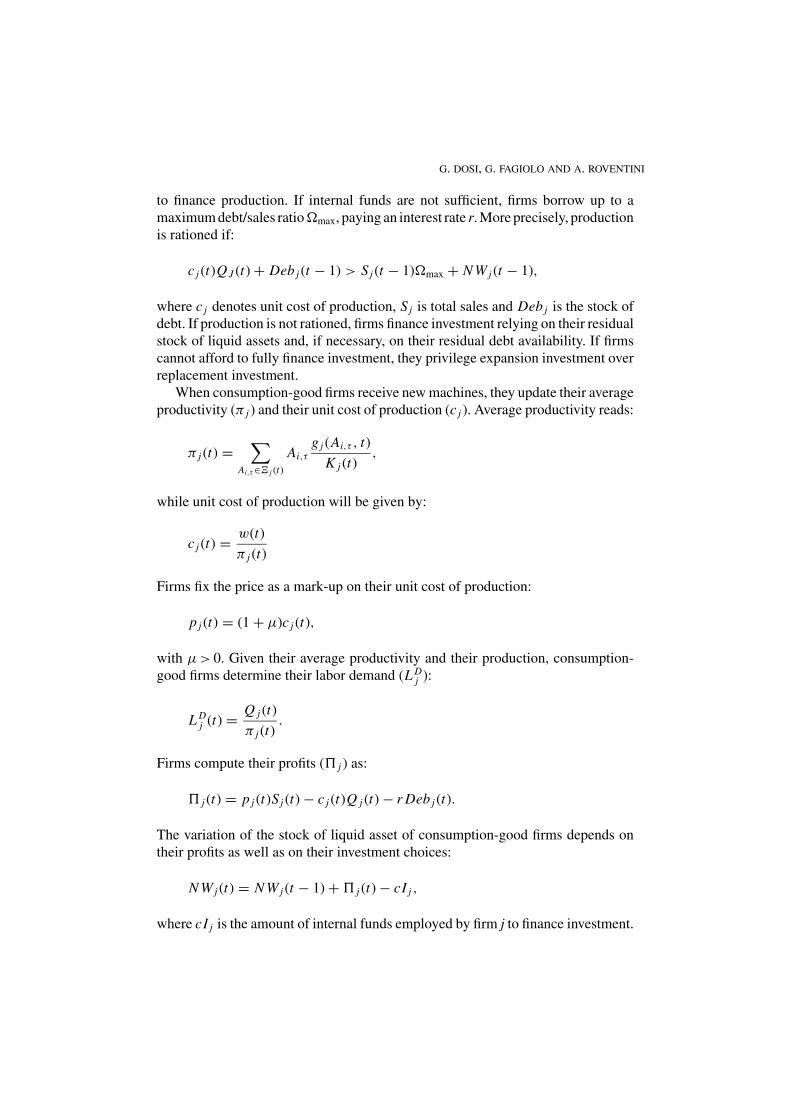
G. DOSI, G. FAGIOLO AND A. ROVENTINI
to finance production. If internal funds are not sufficient, firms borrow up to amaximum debt/sales ratio�max, paying an interest rate r. More precisely, productionis rationed if:
c j (t)Q J (t) + Deb j (t − 1) > Sj (t − 1)�max + N W j (t − 1),
where c j denotes unit cost of production, Sj is total sales and Deb j is the stock ofdebt. If production is not rationed, firms finance investment relying on their residualstock of liquid assets and, if necessary, on their residual debt availability. If firmscannot afford to fully finance investment, they privilege expansion investment overreplacement investment.
When consumption-good firms receive new machines, they update their averageproductivity (π j ) and their unit cost of production (c j ). Average productivity reads:
π j (t) =∑
Ai,τ ∈� j (t)
Ai,τg j (Ai,τ , t)
K j (t),
while unit cost of production will be given by:
c j (t) = w(t)
π j (t)
Firms fix the price as a mark-up on their unit cost of production:
p j (t) = (1 + μ)c j (t),
with μ > 0. Given their average productivity and their production, consumption-good firms determine their labor demand (L D
j ):
L Dj (t) = Q j (t)
π j (t).
Firms compute their profits (� j ) as:
� j (t) = p j (t)Sj (t) − c j (t)Q j (t) − r Deb j (t).
The variation of the stock of liquid asset of consumption-good firms depends ontheir profits as well as on their investment choices:
N W j (t) = N W j (t − 1) + � j (t) − cI j ,
where cI j is the amount of internal funds employed by firm j to finance investment.
AN EVOLUTIONARY MODEL OF ENDOGENOUS BUSINESS CYCLES
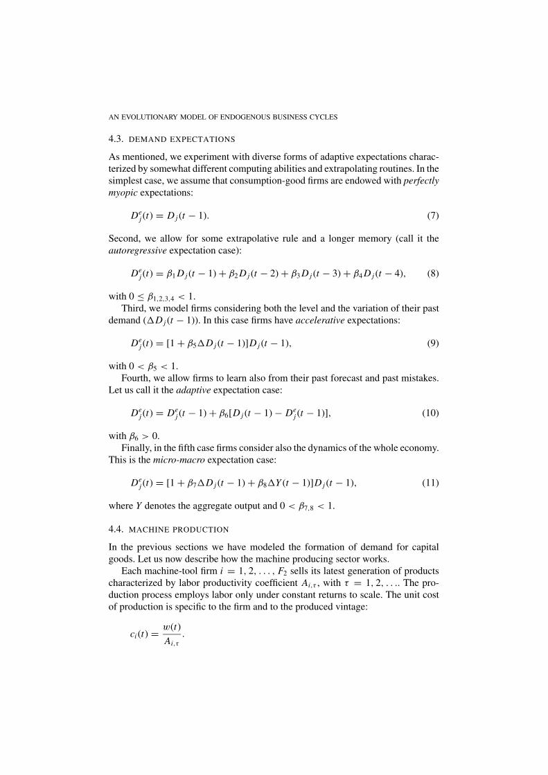
4.3. DEMAND EXPECTATIONS
As mentioned, we experiment with diverse forms of adaptive expectations charac-terized by somewhat different computing abilities and extrapolating routines. In thesimplest case, we assume that consumption-good firms are endowed with perfectlymyopic expectations:
Dej (t) = D j (t − 1). (7)
Second, we allow for some extrapolative rule and a longer memory (call it theautoregressive expectation case):
Dej (t) = β1 D j (t − 1) + β2 D j (t − 2) + β3 D j (t − 3) + β4 D j (t − 4), (8)
with 0 ≤ β1,2,3,4 < 1.Third, we model firms considering both the level and the variation of their past
demand (D j (t − 1)). In this case firms have accelerative expectations:
Dej (t) = [1 + β5D j (t − 1)]D j (t − 1), (9)
with 0 < β5 < 1.Fourth, we allow firms to learn also from their past forecast and past mistakes.
Let us call it the adaptive expectation case:
Dej (t) = De
j (t − 1) + β6[D j (t − 1) − Dej (t − 1)], (10)
with β6 > 0.Finally, in the fifth case firms consider also the dynamics of the whole economy.
This is the micro-macro expectation case:
Dej (t) = [1 + β7D j (t − 1) + β8Y (t − 1)]D j (t − 1), (11)
where Y denotes the aggregate output and 0 < β7,8 < 1.
4.4. MACHINE PRODUCTION
In the previous sections we have modeled the formation of demand for capitalgoods. Let us now describe how the machine producing sector works.
Each machine-tool firm i = 1, 2, . . . , F2 sells its latest generation of productscharacterized by labor productivity coefficient Ai,τ , with τ = 1, 2, . . .. The pro-duction process employs labor only under constant returns to scale. The unit costof production is specific to the firm and to the produced vintage:
ci (t) = w(t)
Ai,τ.
G. DOSI, G. FAGIOLO AND A. ROVENTINI
Firms set the price according to a mark-up (μ) rule:
pi (t) = (1 + μ)ci (t),
where μ ≥ 0.As it happens in the consumption-good industry, machine-tool firms bear the
costs of production before receiving the revenues. They finance production withtheir stock of liquid assets (N Wi ) and if necessary with external funds. Once thelevel of production is determined, firms can hire workers according to:
L Di (t) = Qi (t)
Ai,τ,
where L Di is the labor demand of firm i.
Firm i’s profits (�i ) will be then given by:
�i (t) = [pi (t) − ci (t)]Qi (t) − r Debi (t).
The stock of liquid assets changes according to:
N Wi (t) = N Wi (t − 1) + �i (t).
4.5. THE CONSUMPTION-GOOD MARKET
In this and in the next section we present how the markets for producer- andconsumer goods work. We first consider the consumption-good market.
Since consumption-good firms take their production decisions according totheir demand expectations, they can obviously make mistakes which are revealedby variations in inventories. If in the previous period they produced too much(Q j (t − 1) > D j (t − 1)), they accumulate stocks. On the contrary, if they werenot able to fully satisfy their past demand, their ‘competitiveness’ (E j ) at time t isreduced:
E j (t) = −ω1 p j (t) − ω2l j (t) , (12)
where l j is the level of unfilled demand inherited from the previous period andω1,2 are non-negative parameters. The average sectorial competitiveness (E
j) is
obtained by weighting the competitiveness of each firm with its past market share( f j (t − 1)):
Ej(t) =
F1∑j=1
E j (t) f j (t − 1) .
AN EVOLUTIONARY MODEL OF ENDOGENOUS BUSINESS CYCLES
Under condition of imperfect information, consumers take time to imperfectlyadjust to relative consumption-good prices. Thus, market shares evolve accord-ing to a replicator dynamics. More specifically, the market share of each firmwill grow (shrink) if its competitiveness is above (below) the industry-averagecompetitiveness:
f j (t) = f j (t − 1)
(1 + χ1
E j (t) − Ej(t)
Ej(t)
), (13)
with χ1 ≥ 0.14
Aggregate consumption (cf. section 4.8) shapes the demand-side of the marketand it is allocated to consumption-good firms according to their market share:
D j (t) = C(t) f j (t). (14)
4.6. THE CAPITAL-GOOD MARKET
Let us now turn to the capital-good market. Capital-good firms produce on demand.Hence, since they are always able to fully satisfy their demand, their ‘competitive-ness’ depends on the price they charge and on the productivity of the machines theyoffer:
Ei (t) = −ω3 pi (t) + ω4 Ai,τ , (15)
where ω3 and ω4 are non-negative parameters. As in the consumption-good industry,
average sectoral competitiveness (Ei) and market shares ( fi ) read:
Ei(t) =
F2∑i=1
Ei (t) fi (t − 1)
fi (t) = fi (t − 1)
(1 + χ2
Ei (t) − Ei(t)
Ei(t)
), (16)
with χ2 ≥ 0. Also in this case, since the market is characterized by imperfectinformation, there is inertia in the adjustment process of the market shares.
The demand side of the capital-good market depends on the investment choicesof consumption-good firms. More specifically, final-good firm orders determinethe size of the investment ‘cake’, whose slices (Di ) are allocated according to themarket share of each producers:
Di (t) = I (t) fi (t). (17)
G. DOSI, G. FAGIOLO AND A. ROVENTINI
4.7. ENTRY, EXIT, AND TECHNICAL CHANGE
At the end of every period, firms with zero market shares and/or negative net assetsdie and are replaced by new firms. Hence, the number of firms in both sectorsremain constant across time. In order not to bias the overall dynamics, we startby assuming that each entrant is a random copy of a survived firm (see, however,Section 5 for a discussion on more empirically-plausible entry rules).
As mentioned, our economy is fuelled by a never-ending process of technicalchange. At the end of each period, machine-tool firms try to develop the next gen-eration of their product (i.e. discovering machines with a higher labor productivitycoefficient). The result of their efforts is strongly uncertain: firms develop a proto-type whose labor productivity (Ai,new) may be higher or lower than the one of thecurrently manufactured machine. More formally, we let:
Ai,new = Ai,t (1 + ε), (18)
where ε ∼ U [ι1, ι2]. We also posit that firm i will release the next generation ma-chine only if the latter entails a labor productivity improvement (i.e. Ai,new > Ai,τ ).Finally, if the firm decides to produce the new machine, the index τ is accordinglyincremented by one unit.
4.8. MACRO DYNAMICS
The dynamics generated at the micro-level by individual decisions and interactionmechanisms induces, at the macroeconomic level, a stochastic dynamics for all ag-gregate variables of interest (e.g. output, investment, consumption, unemployment,etc.).
Labor market is not cleared by real wage movements. As a consequence, in-voluntary unemployment may arise. The aggregate supply of labor is exogenous,inelastic and grows at a constant rate (η):
L(t) = L(t − 1)(1 + η).
The aggregate demand of labor is the sum of machine- and consumption-goodfirms’ labor demands:
L D(t) =F1∑
j=1
L Dj +
F2∑i=1
L Di (t).
Hence, aggregate employment (Emp) reads:
Emp(t) = min(L D(t), L(t)). (19)
AN EVOLUTIONARY MODEL OF ENDOGENOUS BUSINESS CYCLES
The wage rate is determined by both institutional and market factors, with bothindexation mechanisms upon consumption prices and average productivity, on theone hand, and, adjustments to unemployment rates, on the others:
w(t) = w(t − 1) +(
1 + ψ1
cpi(t) − cpi(t − 1)
cpi(t − 1)
+ ψ2
A(t) − A(t − 1)
A(t − 1)+ ψ3
U (t) − U (t − 1)
U (t − 1)
), (20)
where cpi is the consumer price index, A is average labor productivity and U is theunemployment rate. The system parameters ψ1,2,3 allow one to characterize variousinstitutional regimes for the labor market.
In addition to the industries producing consumption goods and machines – callthem the tradable sector of the economy – it is reasonable to assume a parallelsource of aggregate demand associated with a non-market sector – including ofcourse in its empirical counterpart government services. In the model, its admittedlyblack-boxed representation is through a contribution to aggregate consumptionproportional to the whole labor force and the aggregate wage bill:
C(t) = w(t)Emp(t) + ϕw(t)L , (21)
with 0 < ϕ < 1.Our model straightforwardly belongs to the evolutionary/ACE class. Since in
general, analytical, closed-form, solutions can hardly be obtained, one must resortto computer simulations to analyze the properties of the (stochastic) processesgoverning the coevolution of micro and macro variables.15
To do so, one should in principle address an extensive Monte Carlo analysisin order to understand how the statistics of interests change together with initialconditions and system parameters. Notice, in any case, that in our model the onlystochastic component affecting the underlying dynamics is given by technologicalimprovements in machine efficiencies. In fact, sensitivity exercises show that theacross-simulation stochastic variability is quite low and no chaotic pattern is de-tected. Hence, we can confidently present below results concerning averages overa limited number of replications (typically M = 50) as a robust proxy for thebehavior of all time-series of interest.
5. Simulation Results
How does the model fare in terms of its ability to account for the empirical regulari-ties presented in sections 2.1 and 2.2? Here we shall present in detail the simulationresults under the ‘perfectly myopic’ scenario and compare them with the results
G. DOSI, G. FAGIOLO AND A. ROVENTINI
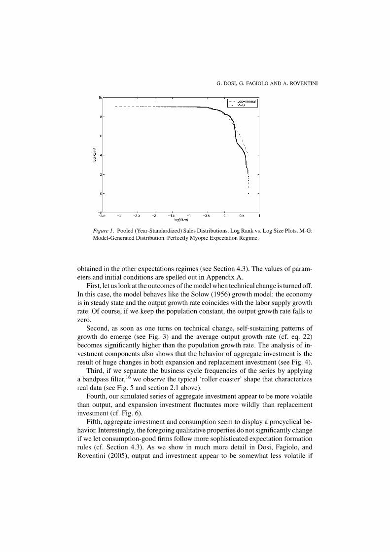
Figure 1. Pooled (Year-Standardized) Sales Distributions. Log Rank vs. Log Size Plots. M-G:
Model-Generated Distribution. Perfectly Myopic Expectation Regime.
obtained in the other expectations regimes (see Section 4.3). The values of param-eters and initial conditions are spelled out in Appendix A.
First, let us look at the outcomes of the model when technical change is turned off.In this case, the model behaves like the Solow (1956) growth model: the economyis in steady state and the output growth rate coincides with the labor supply growthrate. Of course, if we keep the population constant, the output growth rate falls tozero.
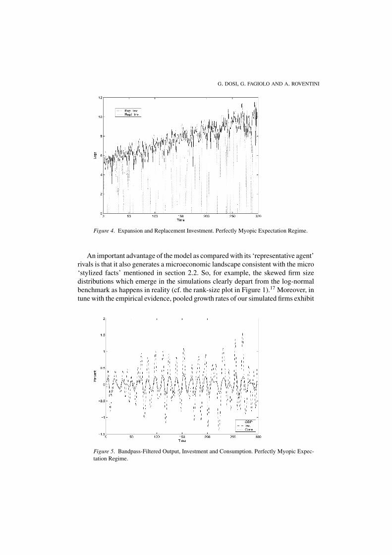
Second, as soon as one turns on technical change, self-sustaining patterns ofgrowth do emerge (see Fig. 3) and the average output growth rate (cf. eq. 22)becomes significantly higher than the population growth rate. The analysis of in-vestment components also shows that the behavior of aggregate investment is theresult of huge changes in both expansion and replacement investment (see Fig. 4).
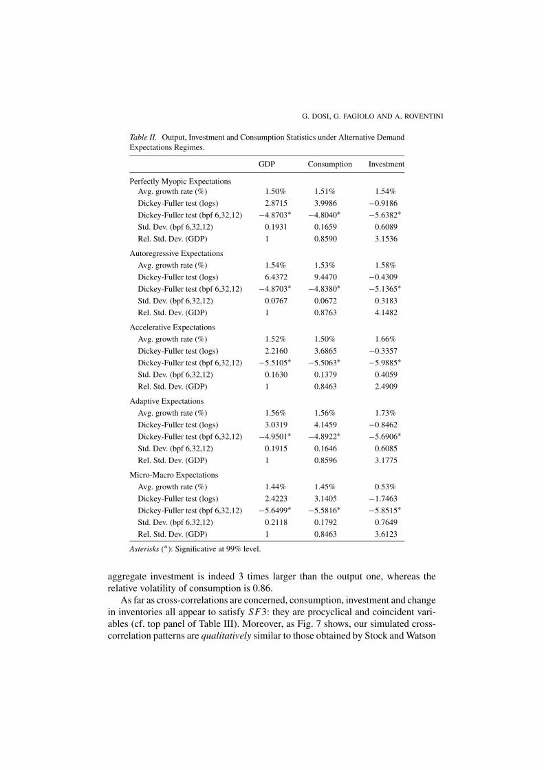
Third, if we separate the business cycle frequencies of the series by applyinga bandpass filter,16 we observe the typical ‘roller coaster’ shape that characterizesreal data (see Fig. 5 and section 2.1 above).
Fourth, our simulated series of aggregate investment appear to be more volatilethan output, and expansion investment fluctuates more wildly than replacementinvestment (cf. Fig. 6).
Fifth, aggregate investment and consumption seem to display a procyclical be-havior. Interestingly, the foregoing qualitative properties do not significantly changeif we let consumption-good firms follow more sophisticated expectation formationrules (cf. Section 4.3). As we show in much more detail in Dosi, Fagiolo, andRoventini (2005), output and investment appear to be somewhat less volatile if
AN EVOLUTIONARY MODEL OF ENDOGENOUS BUSINESS CYCLES
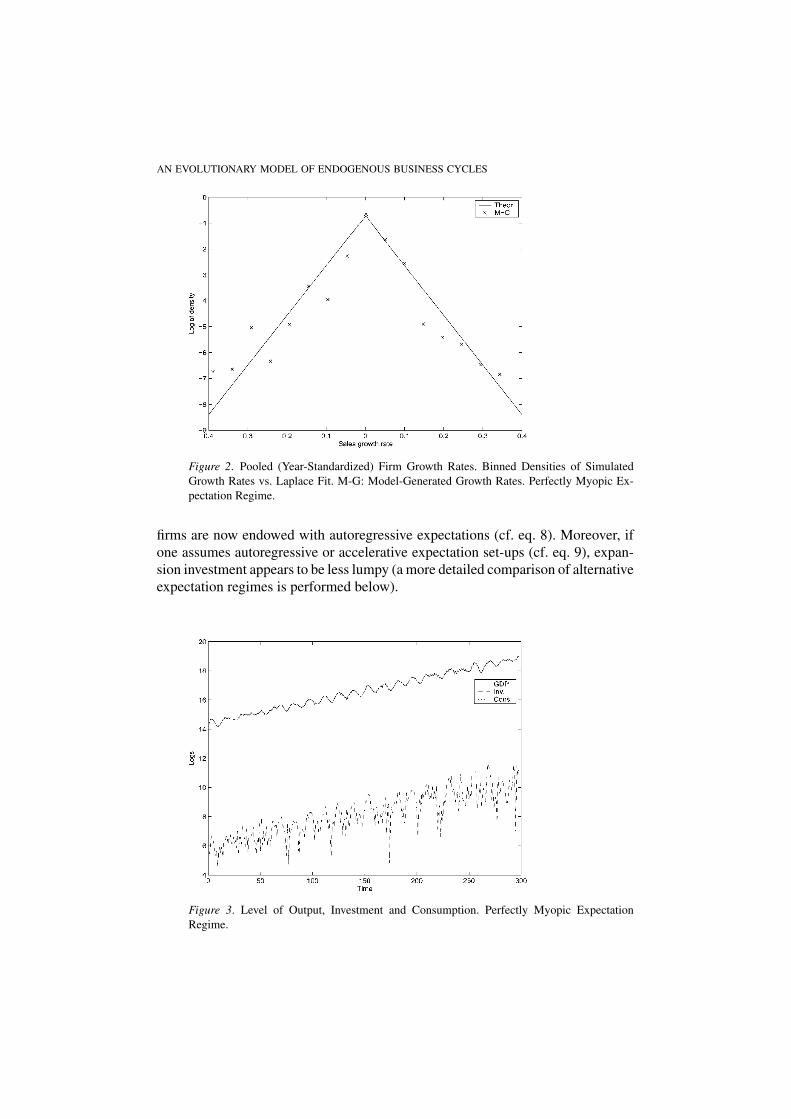
Figure 2. Pooled (Year-Standardized) Firm Growth Rates. Binned Densities of Simulated
Growth Rates vs. Laplace Fit. M-G: Model-Generated Growth Rates. Perfectly Myopic Ex-
pectation Regime.
firms are now endowed with autoregressive expectations (cf. eq. 8). Moreover, ifone assumes autoregressive or accelerative expectation set-ups (cf. eq. 9), expan-sion investment appears to be less lumpy (a more detailed comparison of alternativeexpectation regimes is performed below).
Figure 3. Level of Output, Investment and Consumption. Perfectly Myopic Expectation
Regime.
G. DOSI, G. FAGIOLO AND A. ROVENTINI
Figure 4. Expansion and Replacement Investment. Perfectly Myopic Expectation Regime.
An important advantage of the model as compared with its ‘representative agent’rivals is that it also generates a microeconomic landscape consistent with the micro‘stylized facts’ mentioned in section 2.2. So, for example, the skewed firm sizedistributions which emerge in the simulations clearly depart from the log-normalbenchmark as happens in reality (cf. the rank-size plot in Figure 1).17 Moreover, intune with the empirical evidence, pooled growth rates of our simulated firms exhibit
Figure 5. Bandpass-Filtered Output, Investment and Consumption. Perfectly Myopic Expec-
tation Regime.

AN EVOLUTIONARY MODEL OF ENDOGENOUS BUSINESS CYCLES
Figure 6. Bandpass-Filtered Expansion and Replacement Investment. Perfectly Myopic Ex-
pectation Regime.
the typical ‘tent-shaped’ patterns, characterized by tails fatter than the Gaussianbenchmark (cf. Fig. 2). What is more, if one fits simulated distributions with thefamily of Subbotin densities, the estimated shape-parameter turns out to be veryclose to the one obtained in empirical studies.18
Let us now turn to a more detailed study of our simulated time-series. Morespecifically, let us address the issue whether simulated series of aggregate outputgrowth, investment, consumption, etc. display statistical properties similar to theempirically observed ones (as summarized in SF1 − 4).
We begin by focusing on the average growth rate (AGR) of the economy:
AG RT = log Y (T ) − log Y (0)
T + 1, (22)
where Y denotes aggregate output and compute Dickey-Fuller (DF) tests on output,consumption and investment in order to detect the presence of unit roots in the series.All results refer to averages computed across M = 50 independent simulations.
The average growth rate of output, consumption and investment are strictlypositive (≈1.5%, see top panel of Table II) and DF tests suggest that output, con-sumption, and investment are non-stationary.
We then detrend the time series obtained from simulations with a bandpassfilter (6,32,12) and we compute standard deviations and cross-correlations betweenoutput and the other series.19 Relative standard deviation levels suggest that themodel is able to match SF1 (i.e. investment is considerably more volatile thanoutput) and SF2 (i.e. consumption is less volatile than output). The volatility of
G. DOSI, G. FAGIOLO AND A. ROVENTINI
Table II. Output, Investment and Consumption Statistics under Alternative Demand
Expectations Regimes.
GDP Consumption Investment
Perfectly Myopic Expectations
Avg. growth rate (%) 1.50% 1.51% 1.54%
Dickey-Fuller test (logs) 2.8715 3.9986 −0.9186
Dickey-Fuller test (bpf 6,32,12) −4.8703∗ −4.8040∗ −5.6382∗Std. Dev. (bpf 6,32,12) 0.1931 0.1659 0.6089
Rel. Std. Dev. (GDP) 1 0.8590 3.1536
Autoregressive Expectations
Avg. growth rate (%) 1.54% 1.53% 1.58%
Dickey-Fuller test (logs) 6.4372 9.4470 −0.4309
Dickey-Fuller test (bpf 6,32,12) −4.8703∗ −4.8380∗ −5.1365∗Std. Dev. (bpf 6,32,12) 0.0767 0.0672 0.3183
Rel. Std. Dev. (GDP) 1 0.8763 4.1482
Accelerative Expectations
Avg. growth rate (%) 1.52% 1.50% 1.66%
Dickey-Fuller test (logs) 2.2160 3.6865 −0.3357
Dickey-Fuller test (bpf 6,32,12) −5.5105∗ −5.5063∗ −5.9885∗Std. Dev. (bpf 6,32,12) 0.1630 0.1379 0.4059
Rel. Std. Dev. (GDP) 1 0.8463 2.4909
Adaptive Expectations
Avg. growth rate (%) 1.56% 1.56% 1.73%
Dickey-Fuller test (logs) 3.0319 4.1459 −0.8462
Dickey-Fuller test (bpf 6,32,12) −4.9501∗ −4.8922∗ −5.6906∗Std. Dev. (bpf 6,32,12) 0.1915 0.1646 0.6085
Rel. Std. Dev. (GDP) 1 0.8596 3.1775
Micro-Macro Expectations
Avg. growth rate (%) 1.44% 1.45% 0.53%
Dickey-Fuller test (logs) 2.4223 3.1405 −1.7463
Dickey-Fuller test (bpf 6,32,12) −5.6499∗ −5.5816∗ −5.8515∗Std. Dev. (bpf 6,32,12) 0.2118 0.1792 0.7649
Rel. Std. Dev. (GDP) 1 0.8463 3.6123
Asterisks (∗): Significative at 99% level.
aggregate investment is indeed 3 times larger than the output one, whereas therelative volatility of consumption is 0.86.
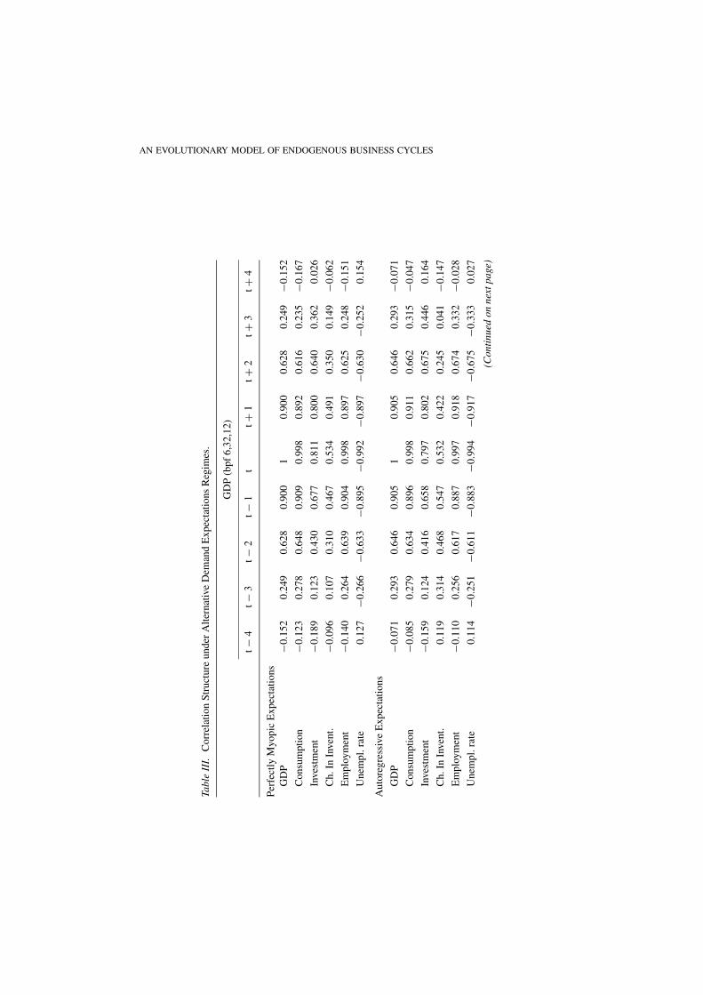
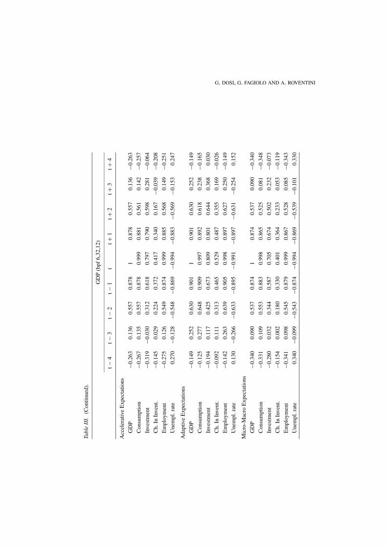
As far as cross-correlations are concerned, consumption, investment and changein inventories all appear to satisfy SF3: they are procyclical and coincident vari-ables (cf. top panel of Table III). Moreover, as Fig. 7 shows, our simulated cross-correlation patterns are qualitatively similar to those obtained by Stock and Watson
AN EVOLUTIONARY MODEL OF ENDOGENOUS BUSINESS CYCLES
Tabl
eII
I.C
orr
elat
ion
Str
uct
ure
un
der
Alt
ern
ativ
eD
eman
dE
xp
ecta
tio
ns
Reg
imes
.
GD
P(b
pf
6,3
2,1
2)
t−
4t−
3t−
2t−
1t
t+
1t+
2t+
3t+
4
Per
fect
lyM
yo
pic
Ex
pec
tati
on
s
GD
P−0
.15
20
.24
90
.62
80
.90
01
0.9
00
0.6
28
0.2
49
−0.1
52
Co
nsu
mp
tio
n−0
.12
30
.27
80
.64
80
.90
90
.99
80
.89
20
.61
60
.23
5−0
.16
7
Inves
tmen
t−0
.18
90
.12
30
.43
00
.67
70
.81
10
.80
00
.64
00
.36
20
.02
6
Ch
.In
Inven
t.−0
.09
60
.10
70
.31
00
.46
70
.53
40
.49
10
.35
00
.14
9−0
.06
2
Em
plo
ym
ent
−0.1
40
0.2
64
0.6
39
0.9
04
0.9
98
0.8
97
0.6
25
0.2
48
−0.1
51
Un
emp
l.ra
te0
.12
7−0
.26
6−0
.63
3−0
.89
5−0
.99
2−0
.89
7−0
.63
0−0
.25
20
.15
4
Au
tore
gre
ssiv
eE
xp
ecta
tio
ns
GD
P−0
.07
10
.29
30
.64
60
.90
51
0.9
05
0.6
46
0.2
93
−0.0
71
Co
nsu
mp
tio
n−0
.08
50
.27
90
.63
40
.89
60
.99
80
.91
10
.66
20
.31
5−0
.04
7
Inves
tmen
t−0
.15
90
.12
40
.41
60
.65
80
.79
70
.80
20
.67
50
.44
60
.16
4
Ch
.In
Inven
t.0
.11
90
.31
40
.46
80
.54
70
.53
20
.42
20
.24
50
.04
1−0
.14
7
Em
plo
ym
ent
−0.1
10
0.2
56
0.6
17
0.8
87
0.9
97
0.9
18
0.6
74
0.3
32
−0.0
28
Un
emp
l.ra
te0
.11
4−0
.25
1−0
.61
1−0
.88
3−0
.99
4−0
.91
7−0
.67
5−0
.33
30
.02
7
(Con
tinu
edon
next
page
)
G. DOSI, G. FAGIOLO AND A. ROVENTINITa
ble
III.
(Co
nti
nu
ed).
GD
P(b
pf
6,3
2,1
2)
t−
4t−
3t−
2t−
1t
t+
1t+
2t+
3t+
4
Acc
eler
ativ
eE
xp
ecta
tio
ns
GD
P−0
.26
30
.13
60
.55
70
.87
81
0.8
78
0.5
57
0.1
36
−0.2
63
Co
nsu
mp
tio
n−0
.26
70
.13
50
.55
70
.87
80
.99
90
.88
10
.56
10
.14
2−0
.25
7
Inves
tmen
t−0
.31
9−0
.03
00
.31
20
.61
80
.79
70
.79
00
.59
80
.28
1−0
.06
4
Ch
.In
Inven
t.−0
.14
50
.02
90
.22
40
.37
20
.41
70
.34
00
.16
7−0
.03
9−0
.20
8
Em
plo
ym
ent
−0.2
75
0.1
26
0.5
49
0.8
74
0.9
99
0.8
85
0.5
68
0.1
49
−0.2
51
Un
emp
l.ra
te0
.27
0−0
.12
8−0
.54
8−0
.86
9−0
.99
4−0
.88
3−0
.56
9−0
.15
30
.24
7
Ad
apti
ve
Ex
pec
tati
on
s
GD
P−0
.14
90
.25
20
.63
00
.90
11
0.9
01
0.6
30
0.2
52
−0.1
49
Co
nsu
mp
tio
n−0
.12
50
.27
70
.64
80
.90
90
.99
70
.89
20
.61
80
.23
8−0
.16
5
Inves
tmen
t−0
.19
40
.11
70
.42
50
.67
30
.80
90
.80
10
.64
40
.36
80
.03
0
Ch
.In
Inven
t.−0
.09
20
.11
10
.31
30
.46
50
.52
90
.48
70
.35
50
.16
9−0
.02
6
Em
plo
ym
ent
−0.1
42
0.2
63
0.6
39
0.9
05
0.9
98
0.8
97
0.6
27
0.2
50
−0.1
49
Un
emp
l.ra
te0
.13
0−0
.26
6−0
.63
3−0
.89
5−0
.99
1−0
.89
7−0
.63
1−0
.25
40
.15
2
Mic
ro-M
acro
Ex
pec
tati
on
s
GD
P−0
.34
00
.09
00
.53
70
.87
41
0.8
74
0.5
37
0.0
90
−0.3
40
Co
nsu
mp
tio
n−0
.33
10
.10
90
.55
30
.88
30
.99
80
.86
50
.52
50
.08
1−0
.34
8
Inves
tmen
t−0
.28
00
.03
20
.34
40
.58
70
.70
50
.67
40
.50
20
.23
2−0
.07
3
Ch
.In
Inven
t.−0
.15
40
.00
20
.18
00
.33
00
.40
10
.36
40
.23
30
.05
3−0
.11
9
Em
plo
ym
ent
−0.3
41
0.0
98
0.5
45
0.8
79
0.9
99
0.8
67
0.5
28
0.0
85
−0.3
43
Un
emp
l.ra
te0
.34
0−0
.09
9−0
.54
3−0
.87
4−0
.99
4−0
.86
9−0
.53
9−0
.10
10
.33
0
AN EVOLUTIONARY MODEL OF ENDOGENOUS BUSINESS CYCLES
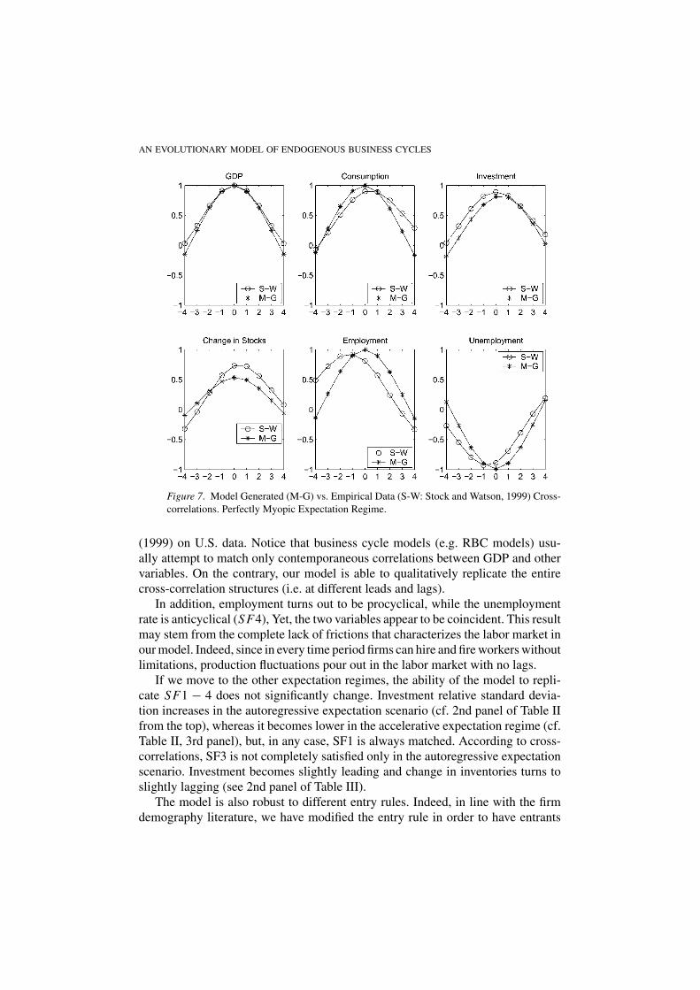
Figure 7. Model Generated (M-G) vs. Empirical Data (S-W: Stock and Watson, 1999) Cross-
correlations. Perfectly Myopic Expectation Regime.
(1999) on U.S. data. Notice that business cycle models (e.g. RBC models) usu-ally attempt to match only contemporaneous correlations between GDP and othervariables. On the contrary, our model is able to qualitatively replicate the entirecross-correlation structures (i.e. at different leads and lags).
In addition, employment turns out to be procyclical, while the unemploymentrate is anticyclical (SF4), Yet, the two variables appear to be coincident. This resultmay stem from the complete lack of frictions that characterizes the labor market inour model. Indeed, since in every time period firms can hire and fire workers withoutlimitations, production fluctuations pour out in the labor market with no lags.
If we move to the other expectation regimes, the ability of the model to repli-cate SF1 − 4 does not significantly change. Investment relative standard devia-tion increases in the autoregressive expectation scenario (cf. 2nd panel of Table IIfrom the top), whereas it becomes lower in the accelerative expectation regime (cf.Table II, 3rd panel), but, in any case, SF1 is always matched. According to cross-correlations, SF3 is not completely satisfied only in the autoregressive expectationscenario. Investment becomes slightly leading and change in inventories turns toslightly lagging (see 2nd panel of Table III).
The model is also robust to different entry rules. Indeed, in line with the firmdemography literature, we have modified the entry rule in order to have entrants
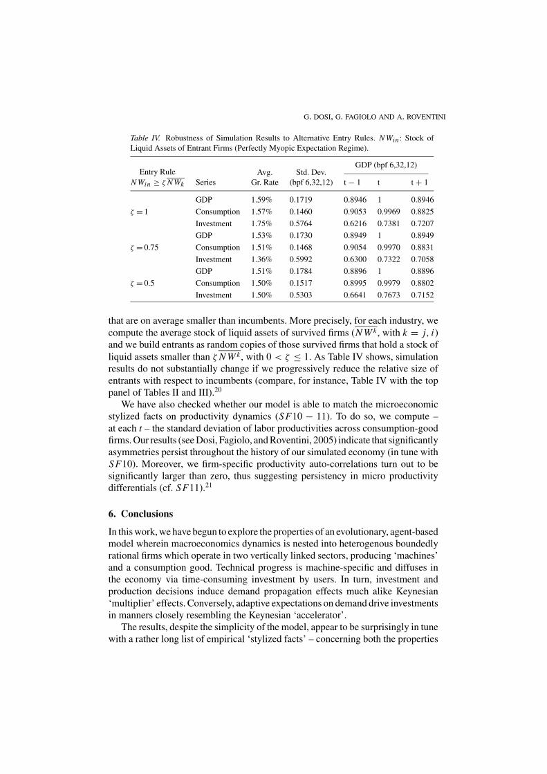
G. DOSI, G. FAGIOLO AND A. ROVENTINI
Table IV. Robustness of Simulation Results to Alternative Entry Rules. N Win : Stock of
Liquid Assets of Entrant Firms (Perfectly Myopic Expectation Regime).
GDP (bpf 6,32,12)Entry Rule
N Win ≥ ζ N Wk Series
Avg.
Gr. Rate
Std. Dev.
(bpf 6,32,12) t − 1 t t + 1
GDP 1.59% 0.1719 0.8946 1 0.8946
ζ = 1 Consumption 1.57% 0.1460 0.9053 0.9969 0.8825
Investment 1.75% 0.5764 0.6216 0.7381 0.7207
GDP 1.53% 0.1730 0.8949 1 0.8949
ζ = 0.75 Consumption 1.51% 0.1468 0.9054 0.9970 0.8831
Investment 1.36% 0.5992 0.6300 0.7322 0.7058
GDP 1.51% 0.1784 0.8896 1 0.8896
ζ = 0.5 Consumption 1.50% 0.1517 0.8995 0.9979 0.8802
Investment 1.50% 0.5303 0.6641 0.7673 0.7152
that are on average smaller than incumbents. More precisely, for each industry, we
compute the average stock of liquid assets of survived firms (N W k , with k = j, i)and we build entrants as random copies of those survived firms that hold a stock of
liquid assets smaller than ζ N W k , with 0 < ζ ≤ 1. As Table IV shows, simulationresults do not substantially change if we progressively reduce the relative size ofentrants with respect to incumbents (compare, for instance, Table IV with the toppanel of Tables II and III).20
We have also checked whether our model is able to match the microeconomicstylized facts on productivity dynamics (SF10 − 11). To do so, we compute –at each t – the standard deviation of labor productivities across consumption-goodfirms. Our results (see Dosi, Fagiolo, and Roventini, 2005) indicate that significantlyasymmetries persist throughout the history of our simulated economy (in tune withSF10). Moreover, we firm-specific productivity auto-correlations turn out to besignificantly larger than zero, thus suggesting persistency in micro productivitydifferentials (cf. SF11).21
6. Conclusions
In this work, we have begun to explore the properties of an evolutionary, agent-basedmodel wherein macroeconomics dynamics is nested into heterogenous boundedlyrational firms which operate in two vertically linked sectors, producing ‘machines’and a consumption good. Technical progress is machine-specific and diffuses inthe economy via time-consuming investment by users. In turn, investment andproduction decisions induce demand propagation effects much alike Keynesian‘multiplier’ effects. Conversely, adaptive expectations on demand drive investmentsin manners closely resembling the Keynesian ‘accelerator’.
The results, despite the simplicity of the model, appear to be surprisingly in tunewith a rather long list of empirical ‘stylized facts’ – concerning both the properties
AN EVOLUTIONARY MODEL OF ENDOGENOUS BUSINESS CYCLES
of aggregate variables and the underlying microeconomics. The overall picturestemming from the simulation results is one where self-sustaining, fluctuating pat-terns of growth emerge out of the interactions among firms operating in marketregimes that strongly depart from perfect competition. Firms undergo a permanentprocess of selection and try to cope – albeit imperfectly – with a turbulent envi-ronment characterized by endogenous demand waves and technological shocks.This in turn induces lumpiness in individual firm growth patterns, with relativelyfrequent episodes of larger- or smaller-than-average growth.
Self-sustained growth comes together with fluctuations in macroeconomic vari-ables characterized by statistical properties similar to the empirically observed one.Interestingly, preliminary investigations appear to suggest that such properties arerelatively independent from the specification of expectation formation. Rather, it isthe heterogeneity among the agents which is crucial to generate dynamic propertiesof the model.
Evolutionary microfoundations – in the form of multiple agents, who are im-perfectly adaptive in their behavior but also able to innovate – are shown to supportmacrodynamics with strong Keynesian features.
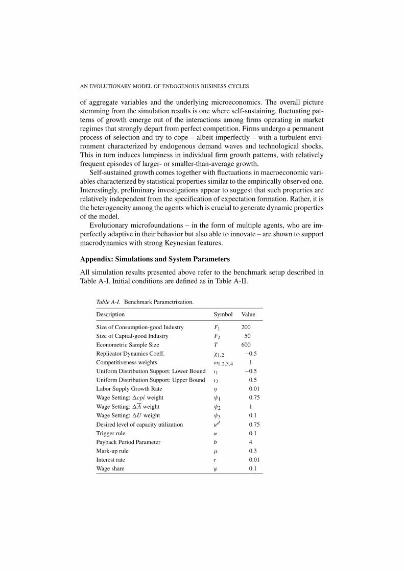
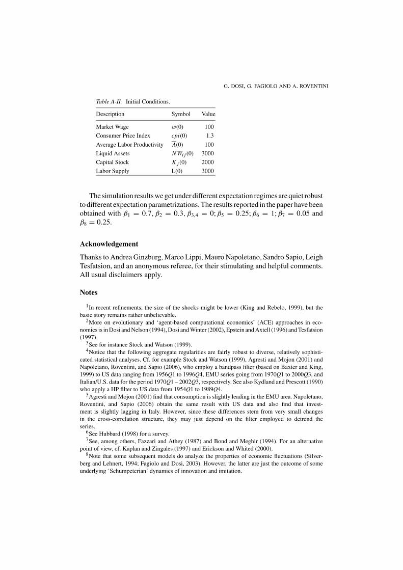
Appendix: Simulations and System Parameters
All simulation results presented above refer to the benchmark setup described inTable A-I. Initial conditions are defined as in Table A-II.
Table A-I. Benchmark Parametrization.
Description Symbol Value
Size of Consumption-good Industry F1 200
Size of Capital-good Industry F2 50
Econometric Sample Size T 600
Replicator Dynamics Coeff. χ1,2 −0.5
Competitiveness weights ω1,2,3,4 1
Uniform Distribution Support: Lower Bound ι1 −0.5
Uniform Distribution Support: Upper Bound ι2 0.5
Labor Supply Growth Rate η 0.01
Wage Setting: cpi weight ψ1 0.75
Wage Setting: A weight ψ2 1
Wage Setting: U weight ψ3 0.1
Desired level of capacity utilization ud 0.75
Trigger rule α 0.1
Payback Period Parameter b 4
Mark-up rule μ 0.3
Interest rate r 0.01
Wage share ϕ 0.1
G. DOSI, G. FAGIOLO AND A. ROVENTINI
Table A-II. Initial Conditions.
Description Symbol Value
Market Wage w(0) 100
Consumer Price Index cpi(0) 1.3
Average Labor Productivity A(0) 100
Liquid Assets N Wi j (0) 3000
Capital Stock K j (0) 2000
Labor Supply L(0) 3000
The simulation results we get under different expectation regimes are quiet robustto different expectation parametrizations. The results reported in the paper have beenobtained with β1 = 0.7, β2 = 0.3, β3,4 = 0; β5 = 0.25; β6 = 1; β7 = 0.05 andβ8 = 0.25.
Acknowledgement
Thanks to Andrea Ginzburg, Marco Lippi, Mauro Napoletano, Sandro Sapio, LeighTesfatsion, and an anonymous referee, for their stimulating and helpful comments.All usual disclaimers apply.
Notes
1In recent refinements, the size of the shocks might be lower (King and Rebelo, 1999), but the
basic story remains rather unbelievable.2More on evolutionary and ‘agent-based computational economics’ (ACE) approaches in eco-
nomics is in Dosi and Nelson (1994), Dosi and Winter (2002), Epstein and Axtell (1996) and Tesfatsion
(1997).3See for instance Stock and Watson (1999).4Notice that the following aggregate regularities are fairly robust to diverse, relatively sophisti-
cated statistical analyses. Cf. for example Stock and Watson (1999), Agresti and Mojon (2001) and
Napoletano, Roventini, and Sapio (2006), who employ a bandpass filter (based on Baxter and King,
1999) to US data ranging from 1956Q1 to 1996Q4, EMU series going from 1970Q1 to 2000Q3, and
Italian/U.S. data for the period 1970Q1 – 2002Q3, respectively. See also Kydland and Prescott (1990)
who apply a HP filter to US data from 1954Q1 to 1989Q4.5Agresti and Mojon (2001) find that consumption is slightly leading in the EMU area. Napoletano,
Roventini, and Sapio (2006) obtain the same result with US data and also find that invest-
ment is slightly lagging in Italy. However, since these differences stem from very small changes
in the cross-correlation structure, they may just depend on the filter employed to detrend the
series.6See Hubbard (1998) for a survey.7See, among others, Fazzari and Athey (1987) and Bond and Meghir (1994). For an alternative
point of view, cf. Kaplan and Zingales (1997) and Erickson and Whited (2000).8Note that some subsequent models do analyze the properties of economic fluctuations (Silver-
berg and Lehnert, 1994; Fagiolo and Dosi, 2003). However, the latter are just the outcome of some
underlying ‘Schumpeterian’ dynamics of innovation and imitation.
AN EVOLUTIONARY MODEL OF ENDOGENOUS BUSINESS CYCLES
9See Caballero (1999) for a discussion. Cf. also Blinder and Maccini (1991) for a survey of (S,s)
inventory behavior models.10An exception is in Thomas (2002). She develops a real business cycle model where firms take their
investment decisions according to a (S,s) rule. However, in this model, lumpy investment does not have
any significant impact at the macro level, because households preferences for smooth consumption
paths sterilize investment lumpiness through price movements (i.e. real wage and interest rate).11This in line with empirical evidence discussed in Feldstein and Foot (1971), Eisner (1972),
Goolsbee (1998), who show that replacement investment is typically not proportional to the capital
stock.12All updating steps are carried out using a ‘parallel updating scheme’. More specifically, all firms
have simultaneously access to the updating step and base their decisions on the most recent observation
of the variables affecting their updating decision.13We assume that there are no secondary markets for capital goods. Hence, firms have no incentives
to reduce their capital stock.14In both consumption- and capital-good markets, a firm dies if its market share ceases to be positive
and market shares of the remaining firms are correspondingly re-adjusted (cf. Dosi et al., 1995).15On the ‘methodology’ of evolutionary/ACE models, see Nelson and Winter (1982), Lane
(1993a,b), Kwasnicki (1998), Dosi and Winter (2002), Pyka and Fagiolo (2005).16See Dosi, Fagiolo, and Roventini (2005) for a discussion of the properties of alternative filtering
techniques.17We employ consumption-good firm sales (S) as a proxy of firm size and we normalize each
observation by the year-average of firm size in order to remove any time trends in our data. This
allows one to get stationary size and growth distributions across years and to safely pool normalized
size distributions. For a similar approach see, among others, Bottazzi, Cefis, and Dosi (2002).18On the theory and empirics of Subbotin fits of firm growth rate distributions, see Bottazzi and
Secchi (2003a,b).19All results refer to the choice of T = 600, cf. Appendix A. This econometric sample size is
sufficient to allow for convergence of recursive moments of all statistics of interest.20Since the net entry rate is zero by definition, an increasing labor supply should force either the
unemployment rate or the average firm size to growth. We find instead that the unemployment rate is
always smaller than one and follows a stationary process, whereas the average firm size grows over
time. Note that the normalization of firm sizes in all our estimates prevent the latter property to bias
firm size distributions.21More precisely, in the last 100 periods of the simulations, we consider the normalized productivity
of firms that survived for at least 40 periods and we compute auto-correlations until lag 6.
References
Agresti, A. and Mojon, B. (2001). Some stylized facts on the euro area business cycle, Working Paper
95, European Central Bank.
Bartelsman, E. and Doms, M. (2000). Understanding productivity: Lessons from longitudinal micro-
data. Journal of Economic Literature, 38, 569–594.
Baxter, M. and King, R. (1999). Measuring business cycle: Approximate band-pass filter for economic
time series. Review of Economics and Statistics, 81, 575–593.
Blinder, A. and Maccini, L. (1991). Taking stock: A critical assessment of recent research on inven-
tories. Journal of Economic Perspectives, 5, 73–96.
Bond, S. and Meghir, C. (1994). Dynamic investment models and the firms financial policy. Reviewof Economic Studies, 61, 197–222.
Bottazzi, G., Cefis, E. and Dosi, G. (2002). Corporate growth and industrial structures: Some evidence
from the Italian manufacturing industry. Industrial and Corporate Change, 11, 705–723.
G. DOSI, G. FAGIOLO AND A. ROVENTINI
Bottazzi, G. and Secchi, A. (2003a). Common properties and sectoral specificities in the dynamics of
U.S. manufacturign firms. Review of Industrial Organization, 23, 217–232.
Bottazzi, G. and Secchi, A. (2003b). Why are distribution of firm growth rates tent-shaped? EconomicLetters, 80, 415–420.
Burns, A.F. and Mitchell, W.C. (1946). Measuring Business Cycles. New York, NBER.
Caballero, R. (1999). Aggregate investment in Taylor, J. and M. Woodford (eds.). Handbook ofMacroeconomics. Amsterdam, Elsevier Science.
Chiaromonte, F. and Dosi, G. (1993). Heterogeneity competition and macroeconomic dynamics.
Structural Change and Economic Dynamics, 4, 39–63.
Cyert, R. and March, J. (1989). A Behavioral Theory of the Firm. 2nd edition, Cambridge, Basil
Blackwell.
Doms, M. and Dunne, T. (1998). Capital adjustment patterns in manufacturing plants. Review Eco-nomic Dynamics, 1, 409–429.
Dosi, G. (1988). Sources procedures and microeconomic effects of innovation. Journal of EconomicLiterature, 26, 126–171.
Dosi, G. and Egidi, M. (1991). Substantive and procedural uncertainty: An exploration of economic
behaviours in changing environments. Journal of Evolutionary Economics, 1, 145–168.
Dosi, G., Fabiani, S., Aversi, R. and Meacci, M. (1994). The Dynamics of international differentiation:
a multi-country evolutionary model. Industrial and Corporate Change, 3, 225–242.
Dosi, G., Fagiolo, G. and Roventini, A. (2005). Animal spirits, lumpy investment and Endogenous
Business Cycles”, Working Paper 2005/04, Laboratory of Economics and Management (LEM),
Sant’Anna School of Advanced Studies, Pisa, Italy.
Dosi, G., Freeman, C. and Fabiani, S. (1994). The process of economic development: Introducing
some stylized facts and theories on technologies, firms and institutions. Industrial and CorporateChange, 3, 1–45.
Dosi, G., Marengo, L. and Fagiolo, G. (2005). Learning in evolutionary environment. in Dopfer, K.
(ed.), Evolutionary Principles of Economics. Cambridge, Cambridge University Press.
Dosi, G., Marsili, O., Orsenigo, L. and Salvatore, R. (1995). Learning, market selection and the
evolution of industrial structures. Small Business Economics, 7, 411–36.
Dosi, G. and Nelson, R. (1994). An introduction to evolutionary theories in economics. Journal ofEvolutionary Economics, 4, 153–172.
Dosi, G. and Winter, S. (2002). Interpreting economic change: Evolution, structures and games
in Augier, M. and J. March (eds.). The Economics of Choice, Change, and Organizations.
Cheltenham, Edward Elgar Publishers.
Eisner, R. (1972). Components of capital expenditures: Replacement and modernization versus ex-
pansion. Review of Economics and Statistics, 54, 297–305.
Epstein, J. and Axtell, R. (1996). Growing Artificial Societies: Social Science from the Bottom-Up.
Washington D.C., MIT Press.
Erickson, T. and Whited, T. (2000). Measurement error and the relationship between investment and
q. Journal of Political Economy, 108, 1027–1057.
Fagiolo, G. and Dosi, G. (2003). Exploitation, exploration and innovation in a model of endogenous
growth with locally interacting agents. Structural Change and Economic Dynamics, 14, 237–
273.
Fazzari, S. and Athey, M. (1987). Asymmetric information, financing constraints, and investments.
Review of Economics and Statistics, 69, 481–487.
Fazzari, S., Hubbard, R. and Petersen, B. (1988). Financing constraints and corporate investment.
Brookings Papers on Economic Activity, 1, 141–195.
Feldstein, M. and Foot, D. (1971). The other half of gross investment: Replacement and modernization
expenditures. Review of Economics and Statistics, 53, 49–58.
Freeman, C. (1982). The Economics of Industrial Innovation. London, Francis Pinter.
AN EVOLUTIONARY MODEL OF ENDOGENOUS BUSINESS CYCLES
Goolsbee, A. (1998). The business cycle, financial performance, and the retirement of capital goods”,
Working Paper 6392, NBER.
Greenwald, B. and Stiglitz, S. (1993). Financial market imperfections and business cycles. QuarterlyJournal of Economics, 108, 77–114.
Hubbard, R. (1998). Capital-market imperfections and investment. Journal of Economic Literature,
36, 193–225.
Kaplan, S. and Zingales, L. (1997). Do investment-cashflow sensitivities provide useful measures of
financing constraints?. Quarterly Journal of Economics, 112, 169–215.
Katona, G. and Morgan, J.N. (1952). The quantitative study of factors determining business decisions.
Quarterly Journal of Economics, 66, 67–90.
King, R. and Rebelo, S. (1999). Resuscitating real business cycles. in Taylor, J. and M. Woodford
(eds.), Handbook of Macroeoconomics. Amsterdam, Elsevier Science.
Kirman, A. (1989). The intrinsic limits of modern economic theory: the emperor has no clothes.
Economic Journal, 99, 126–139.
Kirman, A. (1992). Whom or what does the representative individual represent? Journal of EconomicPerspectives, 6, 117–136.
Kuznets, S. (1930). Secular Movements in Production and Prices. Boston, Houghton Mifflin.
Kwasnicki, W. (1998). Simulation methodology in evolutionary economics. in Schweitzer, F.
and G. Silverberg (eds.), Evolution and Self-Organization in Economics. Berlin, Duncker &
Humbold.
Kydland, F. and Prescott, E. (1990). Business cycles: Real facts and a monetary myth. Federal Reserveof Minneapolis Quarterly Review, Spring 1990, 3–18.
Lane, D.A. (1993a). Artificial worlds and economics, part I. Journal of Evolutionary Economics, 3,
89–107.
Lane, D.A. (1993b). Artificial worlds and economics, Part II. Journal of Evolutionary Economics, 3,
177–97.
Mankiw, G.N. and Romer, D. (eds.) (1991). New Keynesian Economics, Cambridge MA, MIT
Press.
Modigliani, F. and Miller, M. (1958). The cost of capital, corporation finance and the theory of
investment. American Economic Review, 48, 261–297.
Napoletano, M., Roventini, A. and Sapio, S. (2006). Are business cycles all alike? a bandpass filter
analysis of the Italian and US cycles. Rivista Italiana degli Economisti, Forthcoming.
Nelson, R. (1981). Research on productivity growth and productivity difference: Dead ends and new
departures. Journal of Economic Literature, 19, 1029–1064.
Nelson, R. and Winter, S. (1982). An Evolutionary Theory of Economic Change. Cambridge, The
Belknap Press of Harvard University Press.
Pyka, A. and Fagiolo, G. (2005). Agent-based modelling: A methodology for neo-schumpeterian
economics. in Hanusch, H. and A. Pyka (eds.), The Elgar Companion to Neo-SchumpeterianEconomics. Cheltenham, Edward Elgar Publishers.
Rosenberg, N. (1982). Inside the Blackbox. Cambridge, Cambridge University Press.
Rosenberg, N. (1994). Exploring the Black Box : Technology, Economics and History. Cambridge,
Cambridge University Press.
Silverberg, G. and Lehnert, D. (1994). Growth fluctuations in an evolutionary model of creative
destruction. in Silverberg, G. and L. Soete (eds.), The economics of growth and technical change.
Cheltenham, Edward Elgar.
Solow, R.M. (1956). A contribution to the theory of economic growth. Quarterly Journal of Eco-nomics, 70: 65–94.
Stadler, G.W. (1994). Real business cycles. Journal of Economic Literature, 32 (4), 1750–1783.
Stock, J. and Watson, M. (1999). Business cycle fluctuations in U.S. macroeconomic time series. in
Taylor, J. and M. Woodford (eds.), Handbook of Macroeconomics. Amsterdam, Elsevier Science.
G. DOSI, G. FAGIOLO AND A. ROVENTINI
Tesfatsion, L. (1997). How economists can get ALife. in Arthur, W., S. Durlauf and D. Lane (eds.),
The Economy as an Evolving Complex System II. Santa Fe Institute, Santa Fe and Reading, MA,
Addison-Wesley.
Thomas, L. (2002). Is lumpy investment relevant for business cycle? Journal of Political Economy,
110, 508–534.
Zarnowitz, V. (1985). Recent works on business cycles in historical perspectives: A review of theories
and evidence. Journal of Economic Literature, 23, 523–580.
Zarnowitz, V. (1997). Business cycles observed and assessed: Why and how they matter. Working
Paper 6230, NBER.