LANDSAT IMAGE PROCESSING USING ENVI 4.7

Example datasets used in the document are:

1. Pre-Katrina: February 11th 2005. LT50220392005042EDC00/L5022039_03920050211_MTL.txt 2. Post-Katrina: October 25th 2005. LT50220392005298EDC00/L5022039_03920051025_MTL.txt

For convenience purpose we will call pre-katrina data as ‘Dataset-A’ and post-katrina as ‘Dataset-B’. We will be looking into ‘Maximum Likelihood Classification’ algorithm to indentify wetland. For this purpose we will use ‘Dataset-A’ as example below. You can apply the same steps for ‘Dataset-B’ later. There are two methods of atmospheric correction (Dark subtraction & QUAC) as well as two methods for Region of interest selection (polygon method & scatter plot method) have been explained below. -sachin.

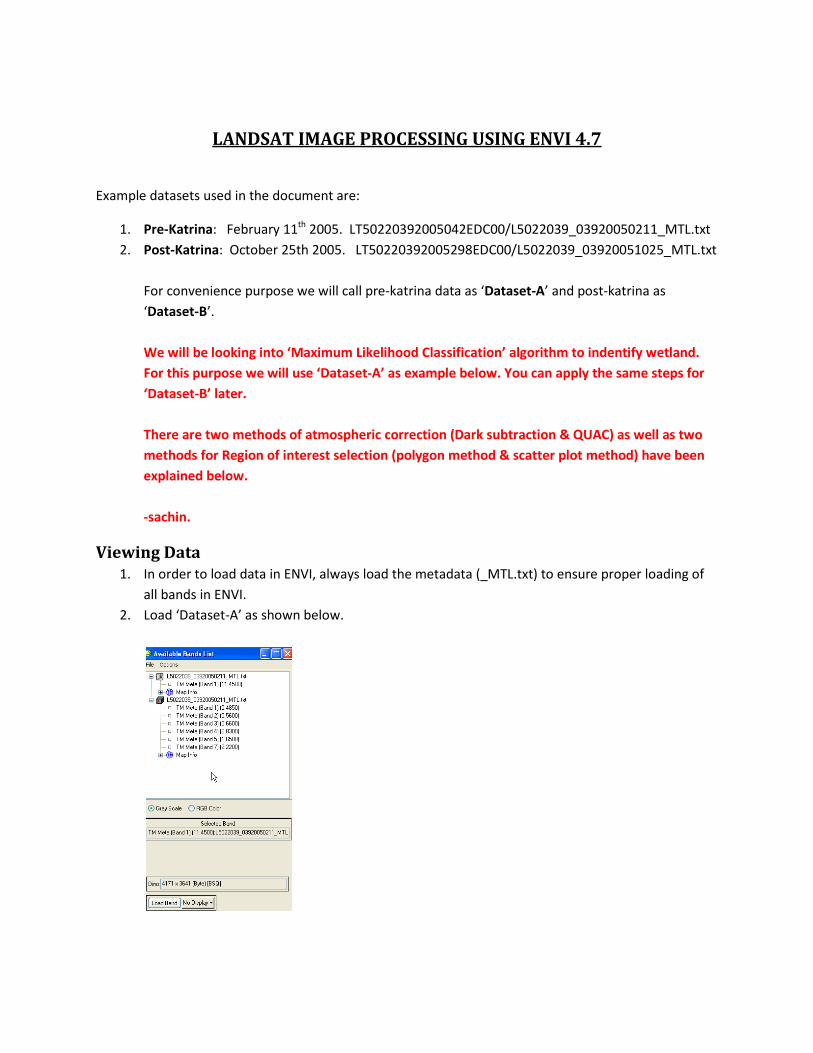
Viewing Data 1. In order to load data in ENVI, always load the metadata (_MTL.txt) to ensure proper loading of

all bands in ENVI. 2. Load ‘Dataset-A’ as shown below.

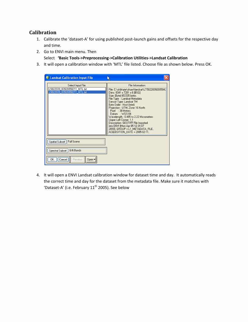
Calibration 1. Calibrate the ‘dataset-A’ for using published post-launch gains and offsets for the respective day

and time. 2. Go to ENVI main menu. Then

Select ‘Basic Tools->Preprocessing->Calibration Utilities->Landsat Calibration 3. It will open a calibration window with ‘MTL’ file listed. Choose file as shown below. Press OK.

4. It will open a ENVI Landsat calibration window for dataset time and day. It automatically reads the correct time and day for the dataset from the metadata file. Make sure it matches with ‘Dataset-A’ (i.e. February 11th 2005). See below

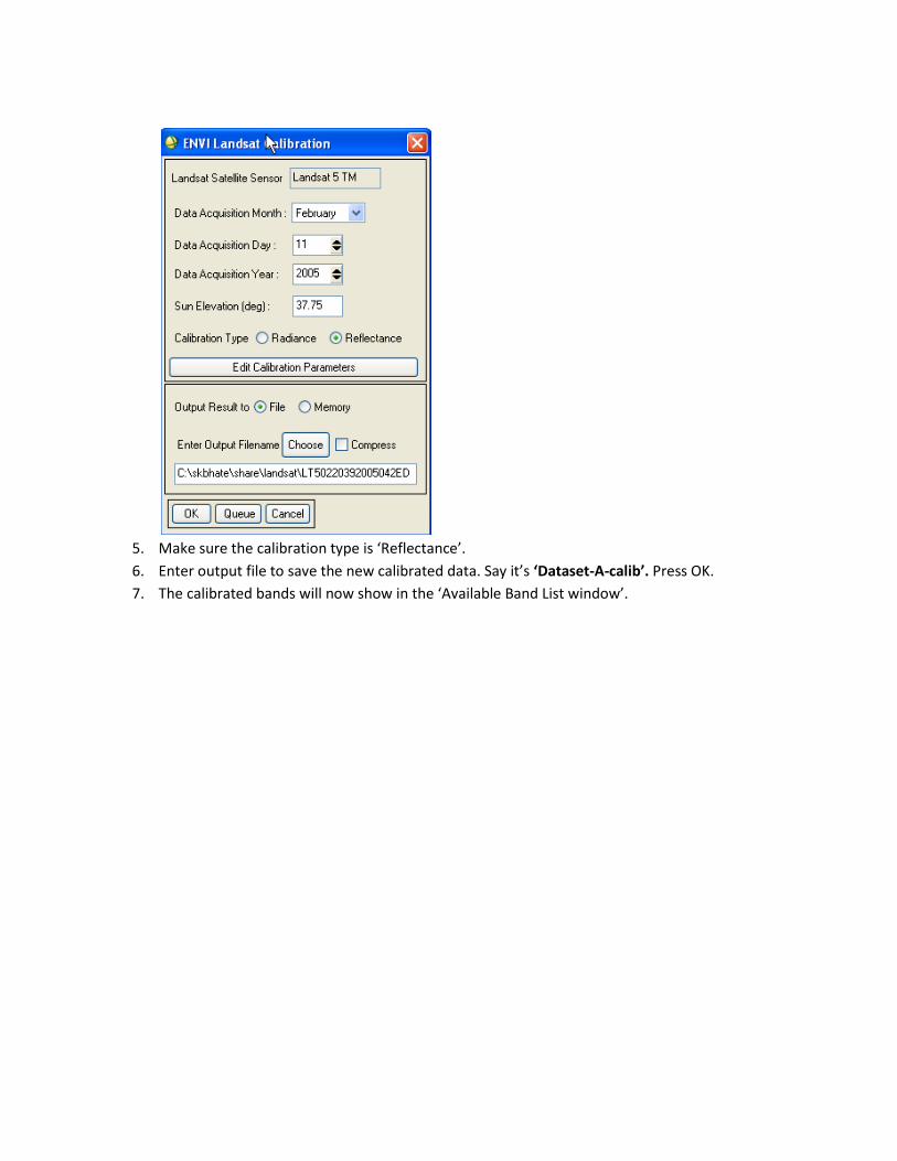
5. Make sure the calibration type is ‘Reflectance’. 6. Enter output file to save the new calibrated data. Say it’s ‘Dataset-A-calib’. Press OK. 7. The calibrated bands will now show in the ‘Available Band List window’.

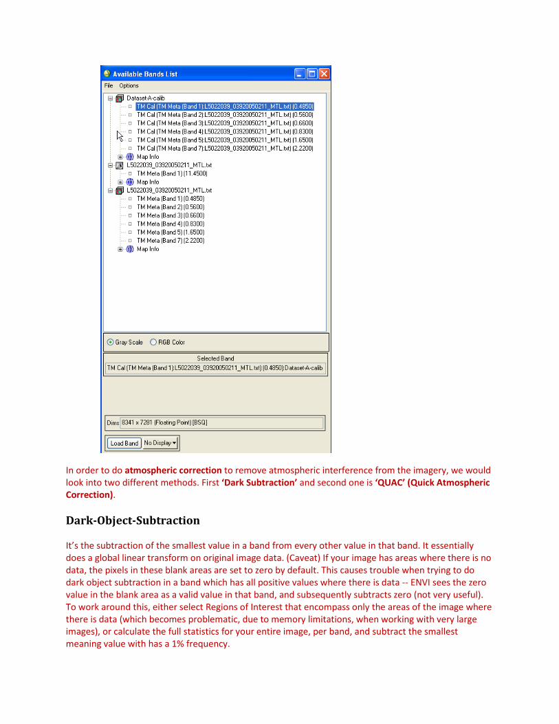
In order to do atmospheric correction to remove atmospheric interference from the imagery, we would look into two different methods. First ‘Dark Subtraction’ and second one is ‘QUAC’ (Quick Atmospheric Correction). Dark-Object-Subtraction It’s the subtraction of the smallest value in a band from every other value in that band. It essentially does a global linear transform on original image data. (Caveat) If your image has areas where there is no data, the pixels in these blank areas are set to zero by default. This causes trouble when trying to do dark object subtraction in a band which has all positive values where there is data -- ENVI sees the zero value in the blank area as a valid value in that band, and subsequently subtracts zero (not very useful). To work around this, either select Regions of Interest that encompass only the areas of the image where there is data (which becomes problematic, due to memory limitations, when working with very large images), or calculate the full statistics for your entire image, per band, and subtract the smallest meaning value with has a 1% frequency.

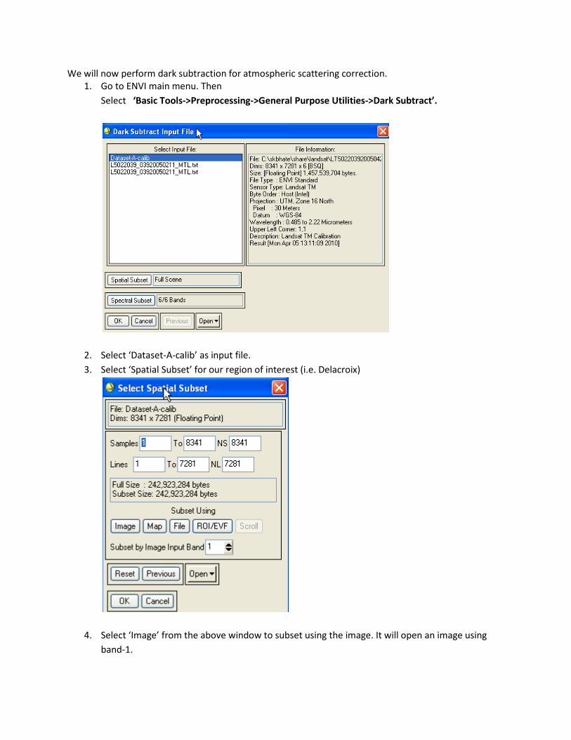
We will now perform dark subtraction for atmospheric scattering correction. 1. Go to ENVI main menu. Then

Select ‘Basic Tools->Preprocessing->General Purpose Utilities->Dark Subtract’.

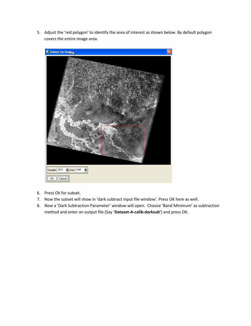
2. Select ‘Dataset-A-calib’ as input file. 3. Select ‘Spatial Subset’ for our region of interest (i.e. Delacroix)

4. Select ‘Image’ from the above window to subset using the image. It will open an image using band-1.

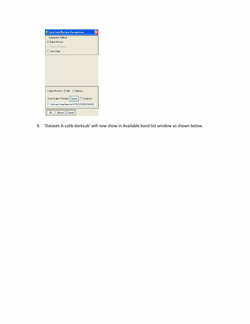
5. Adjust the ‘red polygon’ to identify the area of interest as shown below. By default polygon covers the entire image area.

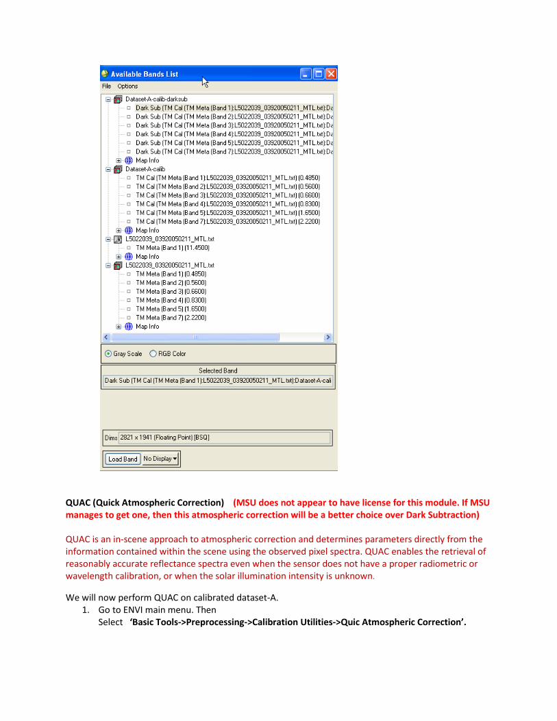
6. Press Ok for subset. 7. Now the subset will show in ‘dark subtract input file window’. Press OK here as well. 8. Now a ‘Dark Subtraction Parameter’ window will open. Choose ‘Band Minimum’ as subtraction

method and enter an output file (Say ‘Dataset-A-calib-darksub’) and press OK.

9. ‘Dataset-A-calib-darksub’ will now show in Available band list window as shown below.

QUAC (Quick Atmospheric Correction) (MSU does not appear to have license for this module. If MSU manages to get one, then this atmospheric correction will be a better choice over Dark Subtraction) QUAC is an in-scene approach to atmospheric correction and determines parameters directly from the information contained within the scene using the observed pixel spectra. QUAC enables the retrieval of reasonably accurate reflectance spectra even when the sensor does not have a proper radiometric or wavelength calibration, or when the solar illumination intensity is unknown. We will now perform QUAC on calibrated dataset-A.

1. Go to ENVI main menu. Then Select ‘Basic Tools->Preprocessing->Calibration Utilities->Quic Atmospheric Correction’.

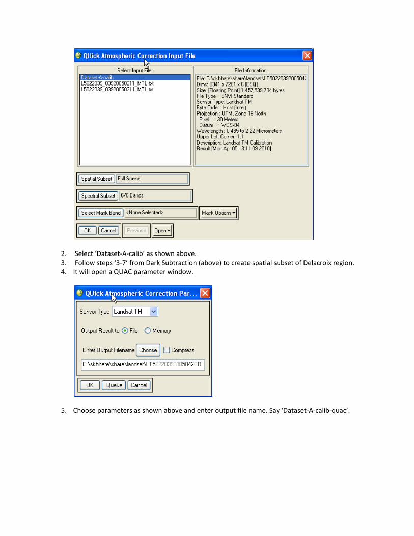
2. Select ‘Dataset-A-calib’ as shown above. 3. Follow steps ‘3-7’ from Dark Subtraction (above) to create spatial subset of Delacroix region. 4. It will open a QUAC parameter window.

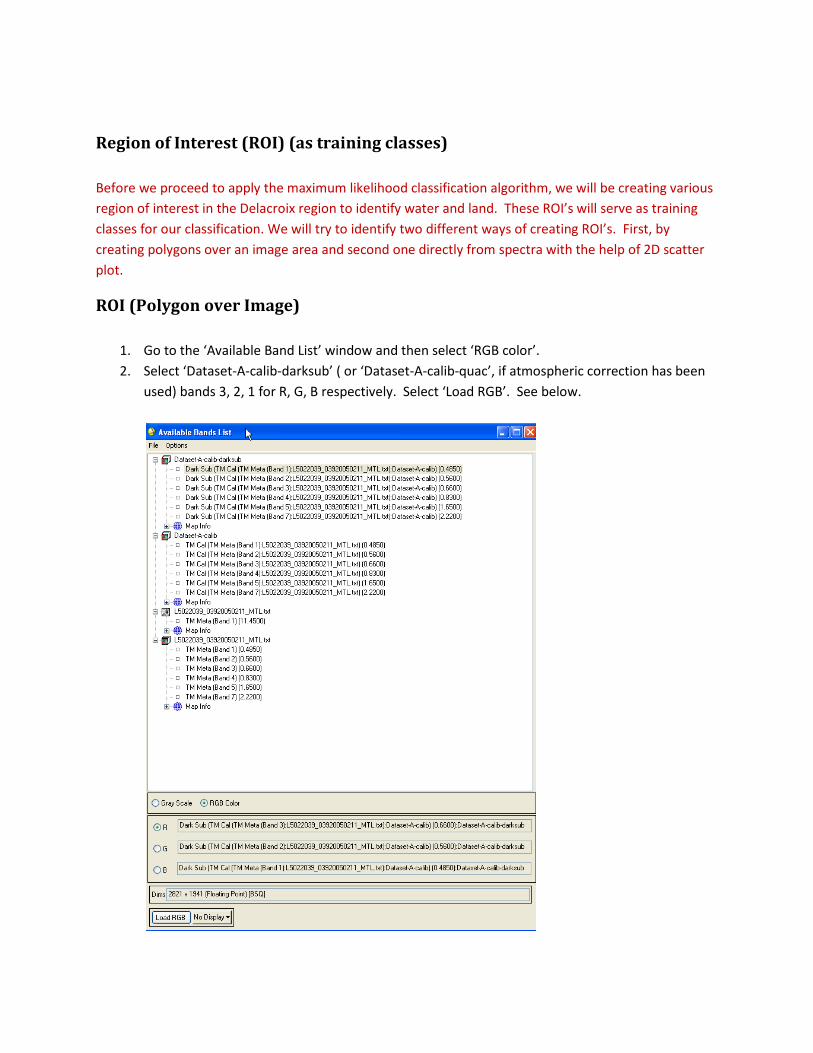
5. Choose parameters as shown above and enter output file name. Say ‘Dataset-A-calib-quac’.

Region of Interest (ROI) (as training classes) Before we proceed to apply the maximum likelihood classification algorithm, we will be creating various region of interest in the Delacroix region to identify water and land. These ROI’s will serve as training classes for our classification. We will try to identify two different ways of creating ROI’s. First, by creating polygons over an image area and second one directly from spectra with the help of 2D scatter plot.

ROI (Polygon over Image)

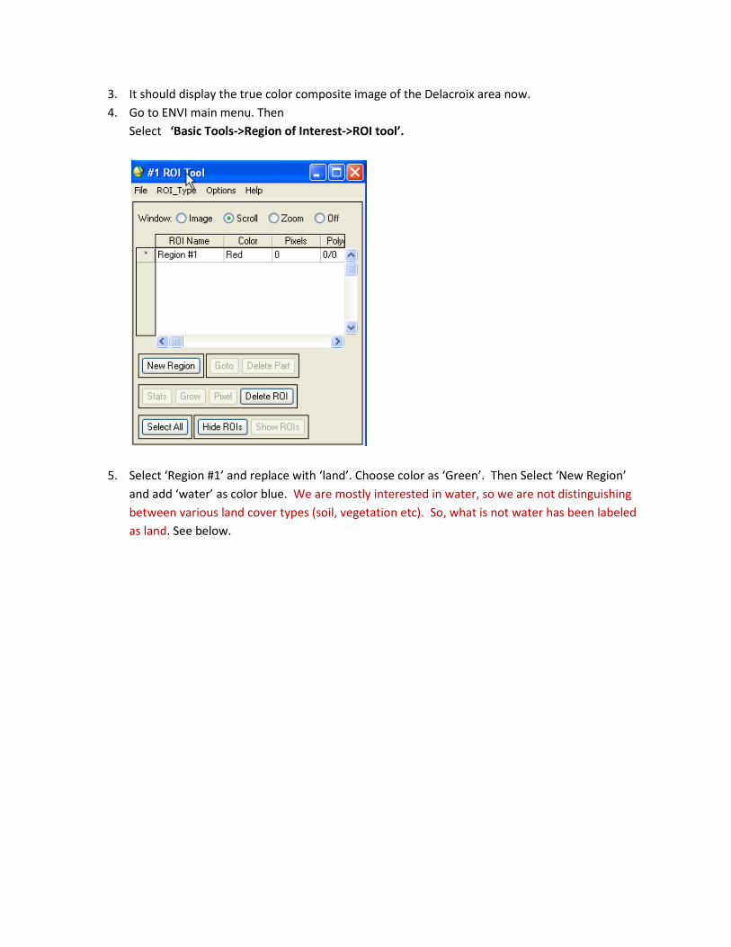
1. Go to the ‘Available Band List’ window and then select ‘RGB color’. 2. Select ‘Dataset-A-calib-darksub’ ( or ‘Dataset-A-calib-quac’, if atmospheric correction has been

used) bands 3, 2, 1 for R, G, B respectively. Select ‘Load RGB’. See below.

3. It should display the true color composite image of the Delacroix area now. 4. Go to ENVI main menu. Then

Select ‘Basic Tools->Region of Interest->ROI tool’.

5. Select ‘Region #1’ and replace with ‘land’. Choose color as ‘Green’. Then Select ‘New Region’ and add ‘water’ as color blue. We are mostly interested in water, so we are not distinguishing between various land cover types (soil, vegetation etc). So, what is not water has been labeled as land. See below.

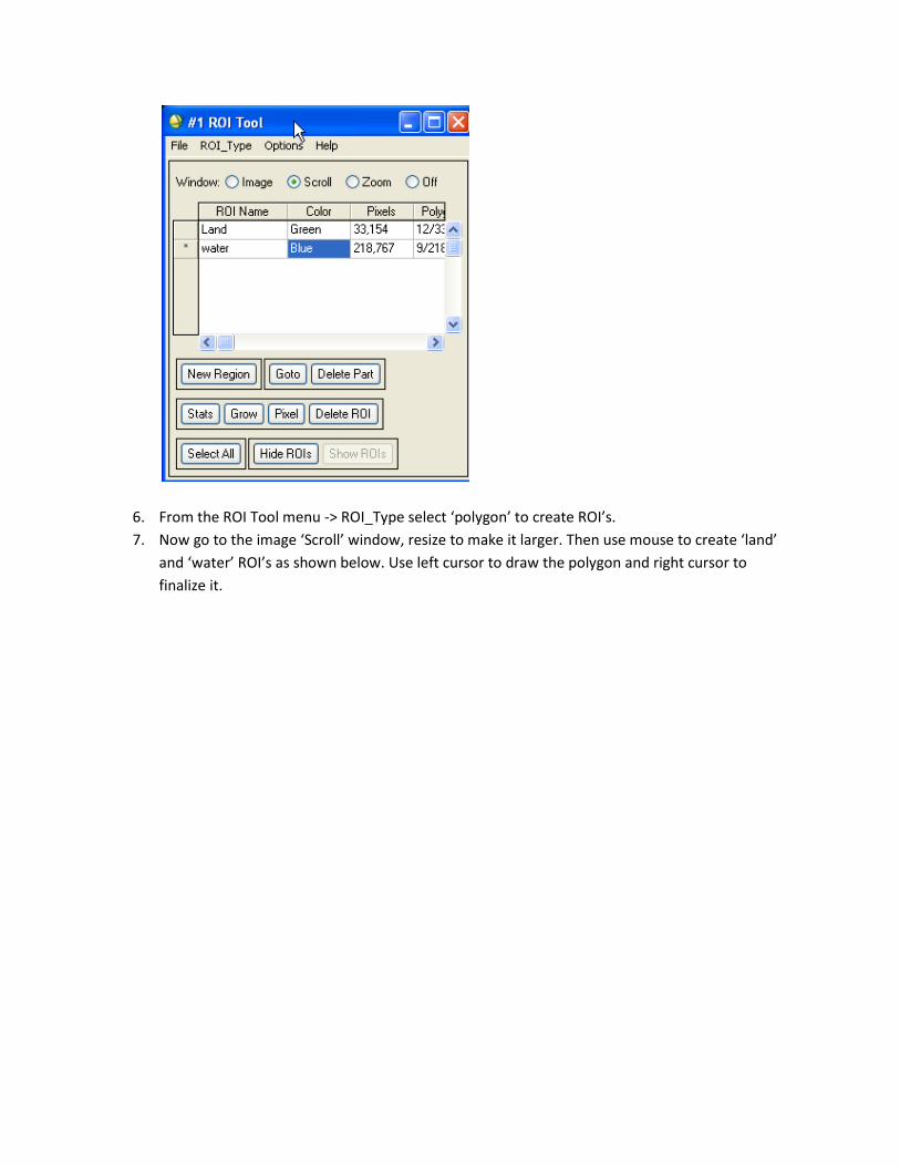
6. From the ROI Tool menu -> ROI_Type select ‘polygon’ to create ROI’s. 7. Now go to the image ‘Scroll’ window, resize to make it larger. Then use mouse to create ‘land’

and ‘water’ ROI’s as shown below. Use left cursor to draw the polygon and right cursor to finalize it.

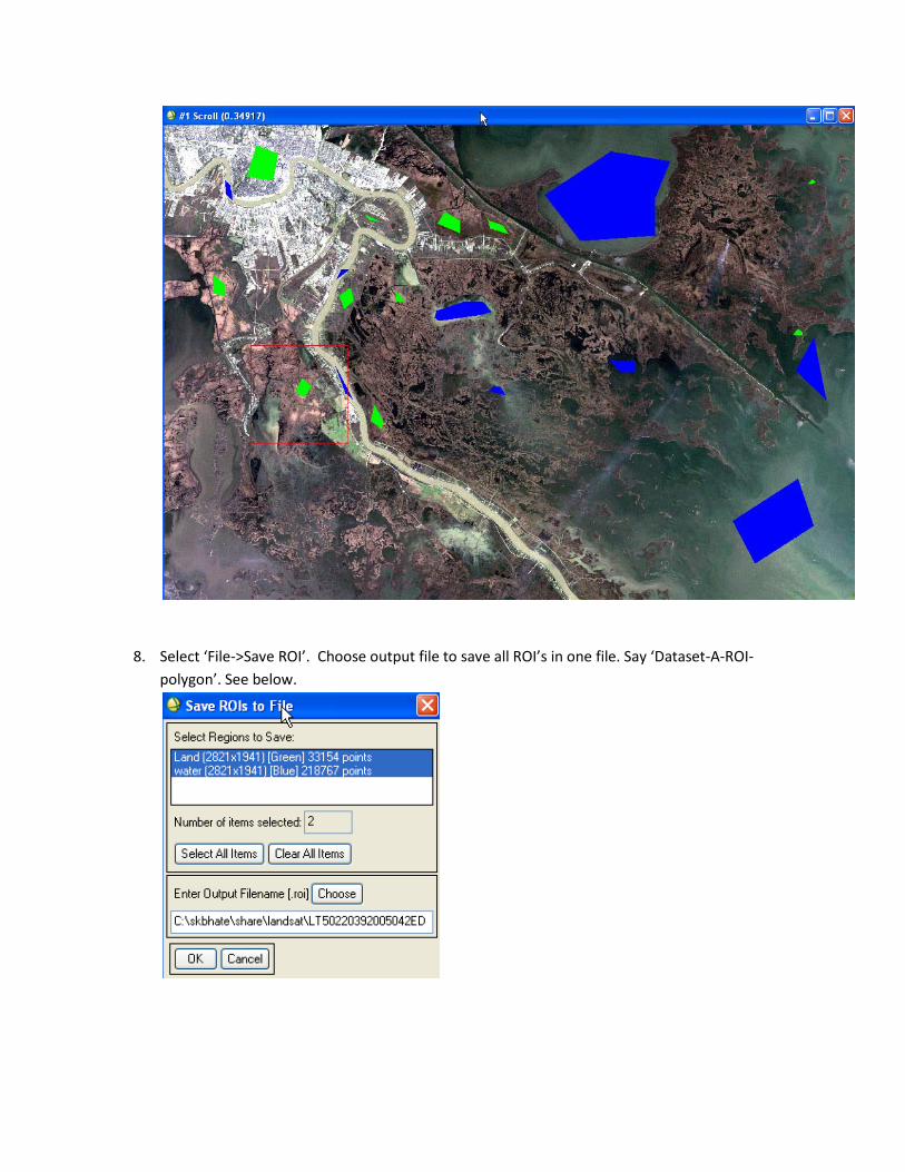
8. Select ‘File->Save ROI’. Choose output file to save all ROI’s in one file. Say ‘Dataset-A-ROI-polygon’. See below.

ROI (using 2D scatter plot)

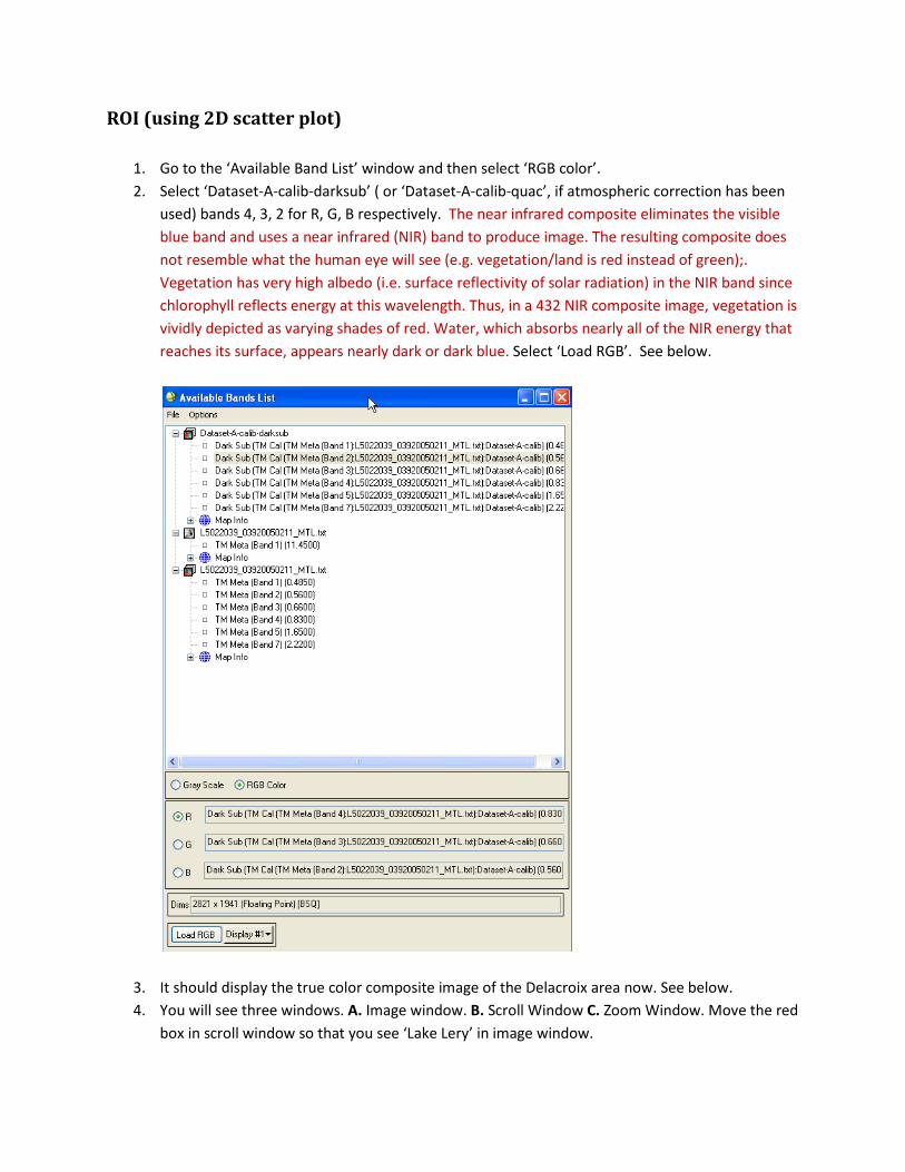
1. Go to the ‘Available Band List’ window and then select ‘RGB color’. 2. Select ‘Dataset-A-calib-darksub’ ( or ‘Dataset-A-calib-quac’, if atmospheric correction has been

used) bands 4, 3, 2 for R, G, B respectively. The near infrared composite eliminates the visible blue band and uses a near infrared (NIR) band to produce image. The resulting composite does not resemble what the human eye will see (e.g. vegetation/land is red instead of green);. Vegetation has very high albedo (i.e. surface reflectivity of solar radiation) in the NIR band since chlorophyll reflects energy at this wavelength. Thus, in a 432 NIR composite image, vegetation is vividly depicted as varying shades of red. Water, which absorbs nearly all of the NIR energy that reaches its surface, appears nearly dark or dark blue. Select ‘Load RGB’. See below.

3. It should display the true color composite image of the Delacroix area now. See below. 4. You will see three windows. A. Image window. B. Scroll Window C. Zoom Window. Move the red

box in scroll window so that you see ‘Lake Lery’ in image window.

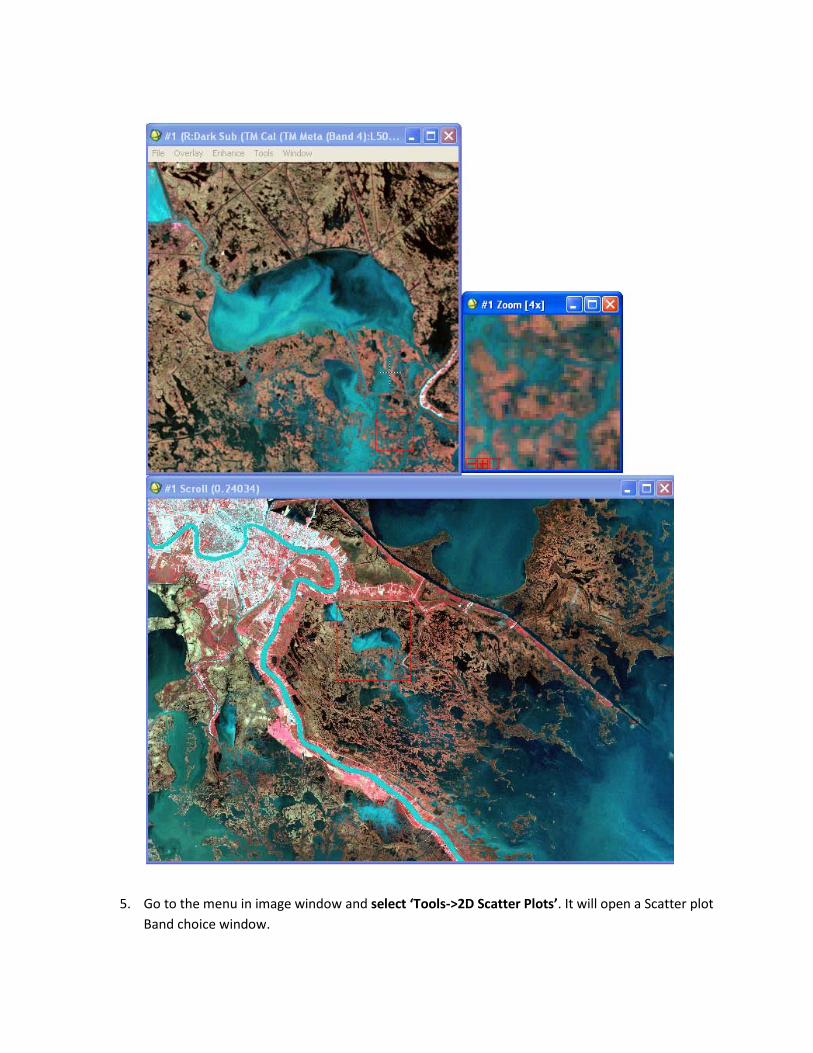
5. Go to the menu in image window and select ‘Tools->2D Scatter Plots’. It will open a Scatter plot Band choice window.

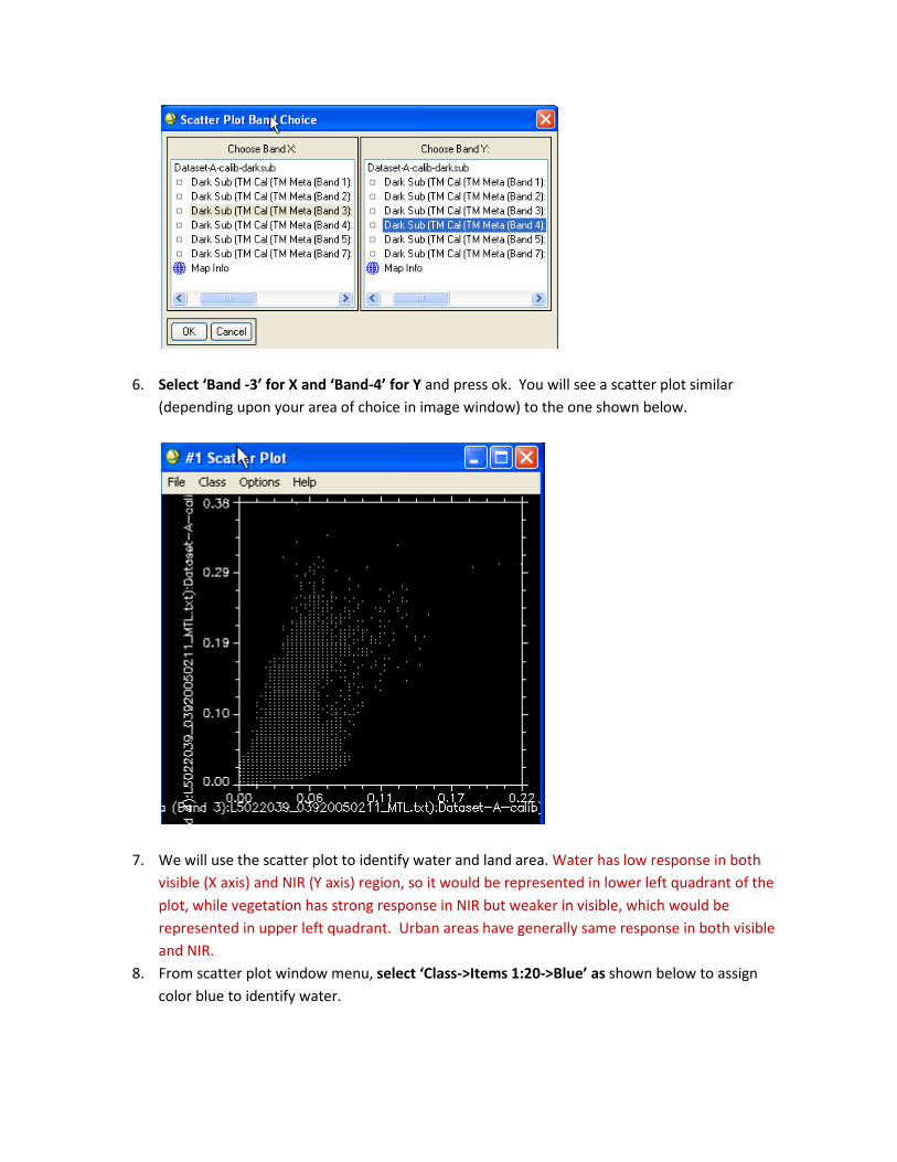
6. Select ‘Band -3’ for X and ‘Band-4’ for Y and press ok. You will see a scatter plot similar (depending upon your area of choice in image window) to the one shown below.

7. We will use the scatter plot to identify water and land area. Water has low response in both visible (X axis) and NIR (Y axis) region, so it would be represented in lower left quadrant of the plot, while vegetation has strong response in NIR but weaker in visible, which would be represented in upper left quadrant. Urban areas have generally same response in both visible and NIR.

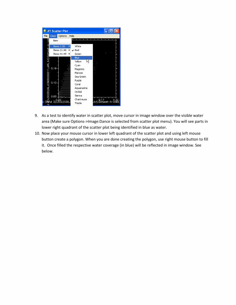
8. From scatter plot window menu, select ‘Class->Items 1:20->Blue’ as shown below to assign color blue to identify water.

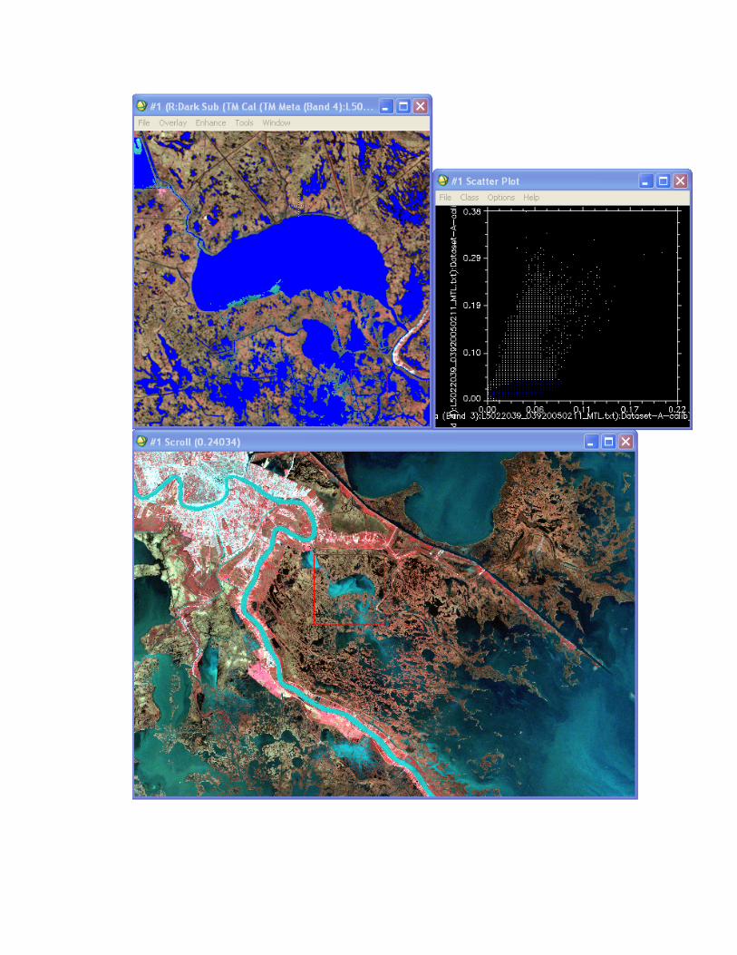
9. As a test to identify water in scatter plot, move cursor in image window over the visible water area (Make sure Options->Image:Dance is selected from scatter plot menu). You will see parts in lower right quadrant of the scatter plot being identified in blue as water.

10. Now place your mouse cursor in lower left quadrant of the scatter plot and using left mouse button create a polygon. When you are done creating the polygon, use right mouse button to fill it. Once filled the respective water coverage (in blue) will be reflected in image window. See below.

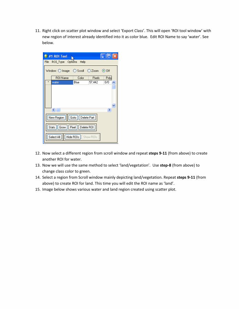
11. Right click on scatter plot window and select ‘Export Class’. This will open ‘ROI tool window’ with new region of interest already identified into it as color blue. Edit ROI Name to say ‘water’. See below.

12. Now select a different region from scroll window and repeat steps 9-11 (from above) to create another ROI for water.

13. Now we will use the same method to select ‘land/vegetation’. Use step-8 (from above) to change class color to green.

14. Select a region from Scroll window mainly depicting land/vegetation. Repeat steps 9-11 (from above) to create ROI for land. This time you will edit the ROI name as ‘land’.

15. Image below shows various water and land region created using scatter plot.

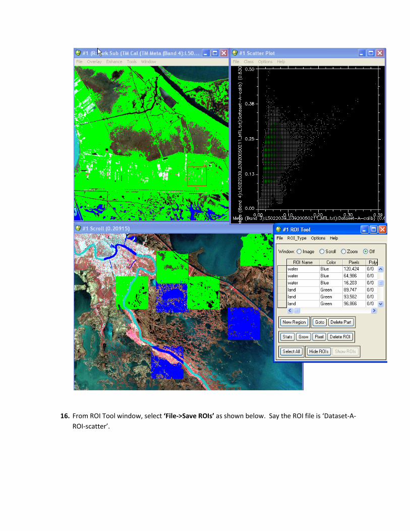
16. From ROI Tool window, select ‘File->Save ROIs’ as shown below. Say the ROI file is ‘Dataset-A-ROI-scatter’.

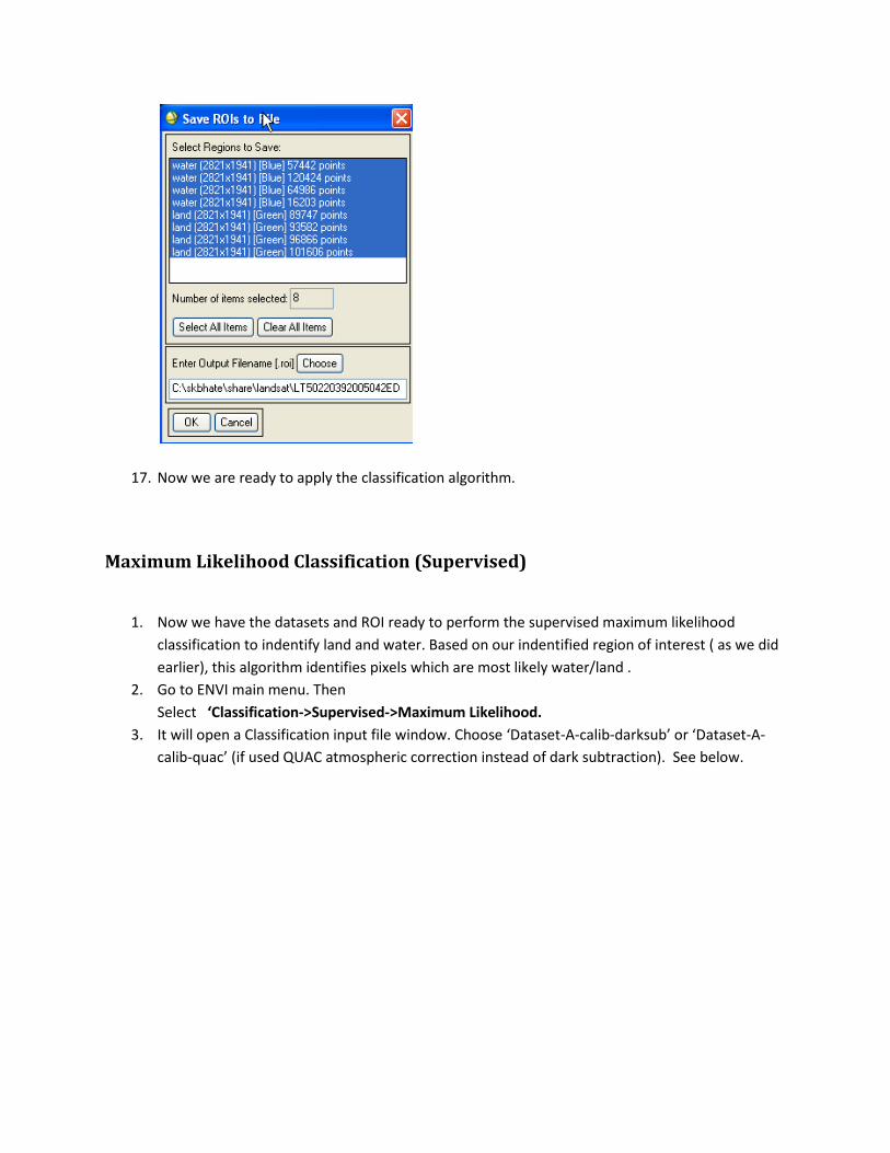
17. Now we are ready to apply the classification algorithm.

Maximum Likelihood Classification (Supervised)

1. Now we have the datasets and ROI ready to perform the supervised maximum likelihood classification to indentify land and water. Based on our indentified region of interest ( as we did earlier), this algorithm identifies pixels which are most likely water/land .

2. Go to ENVI main menu. Then Select ‘Classification->Supervised->Maximum Likelihood.

3. It will open a Classification input file window. Choose ‘Dataset-A-calib-darksub’ or ‘Dataset-A-calib-quac’ (if used QUAC atmospheric correction instead of dark subtraction). See below.

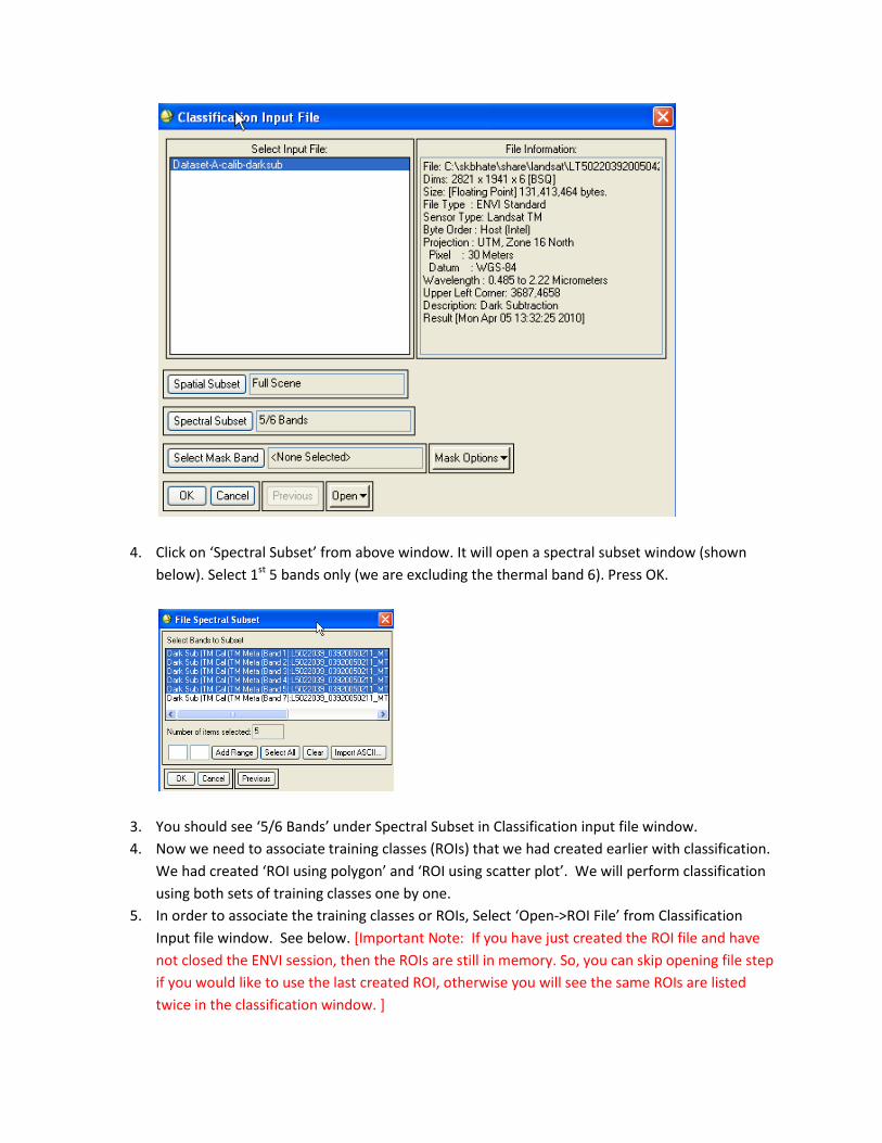
4. Click on ‘Spectral Subset’ from above window. It will open a spectral subset window (shown below). Select 1st 5 bands only (we are excluding the thermal band 6). Press OK.

3. You should see ‘5/6 Bands’ under Spectral Subset in Classification input file window. 4. Now we need to associate training classes (ROIs) that we had created earlier with classification.

We had created ‘ROI using polygon’ and ‘ROI using scatter plot’. We will perform classification using both sets of training classes one by one.

5. In order to associate the training classes or ROIs, Select ‘Open->ROI File’ from Classification Input file window. See below. [Important Note: If you have just created the ROI file and have not closed the ENVI session, then the ROIs are still in memory. So, you can skip opening file step if you would like to use the last created ROI, otherwise you will see the same ROIs are listed twice in the classification window. ]

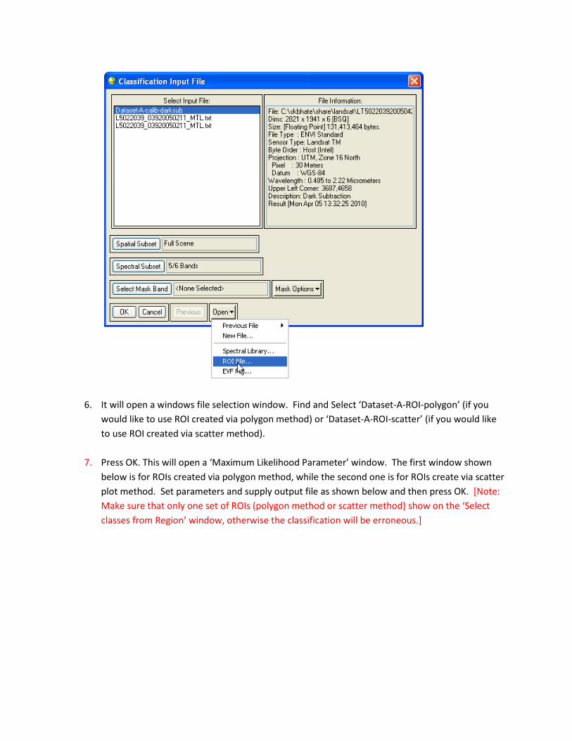
6. It will open a windows file selection window. Find and Select ‘Dataset-A-ROI-polygon’ (if you would like to use ROI created via polygon method) or ‘Dataset-A-ROI-scatter’ (if you would like to use ROI created via scatter method).

7. Press OK. This will open a ‘Maximum Likelihood Parameter’ window. The first window shown below is for ROIs created via polygon method, while the second one is for ROIs create via scatter plot method. Set parameters and supply output file as shown below and then press OK. [Note: Make sure that only one set of ROIs (polygon method or scatter method) show on the ‘Select classes from Region’ window, otherwise the classification will be erroneous.]

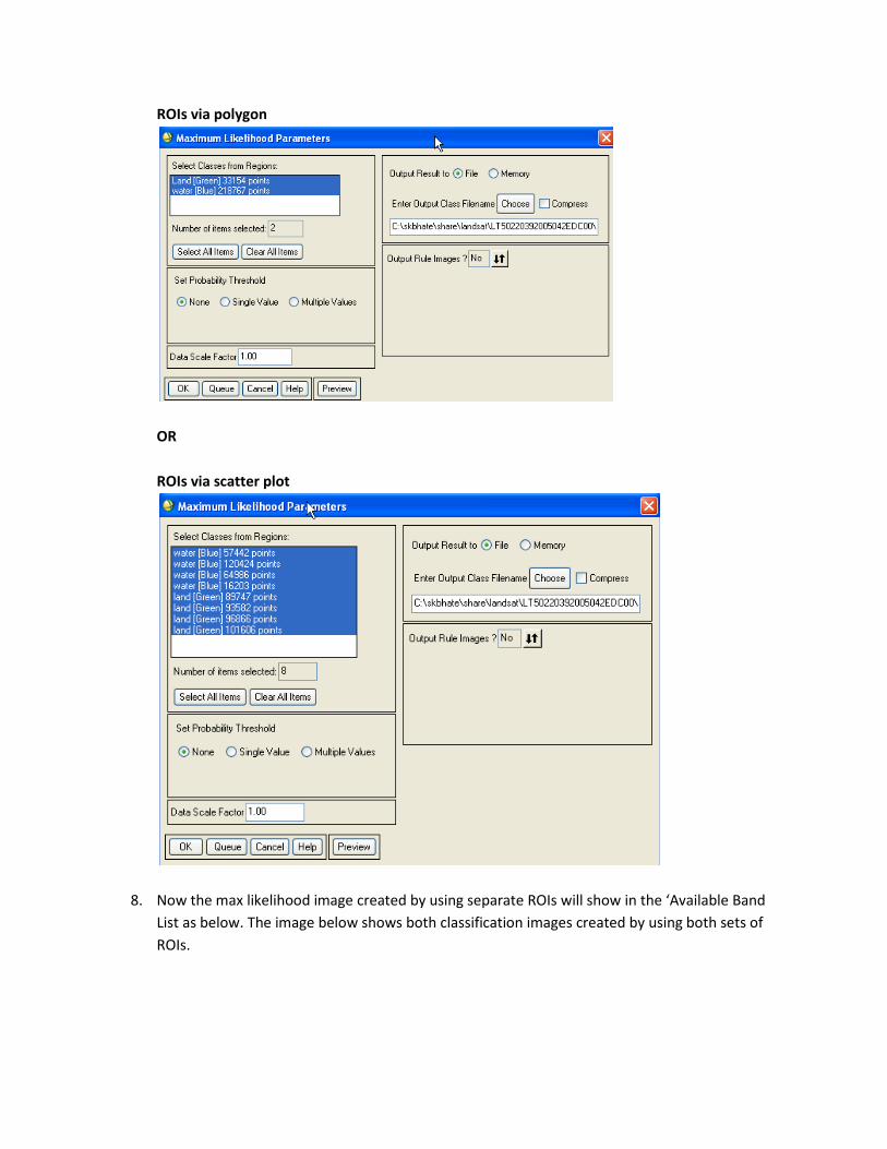
ROIs via polygon

OR ROIs via scatter plot

8. Now the max likelihood image created by using separate ROIs will show in the ‘Available Band List as below. The image below shows both classification images created by using both sets of ROIs.

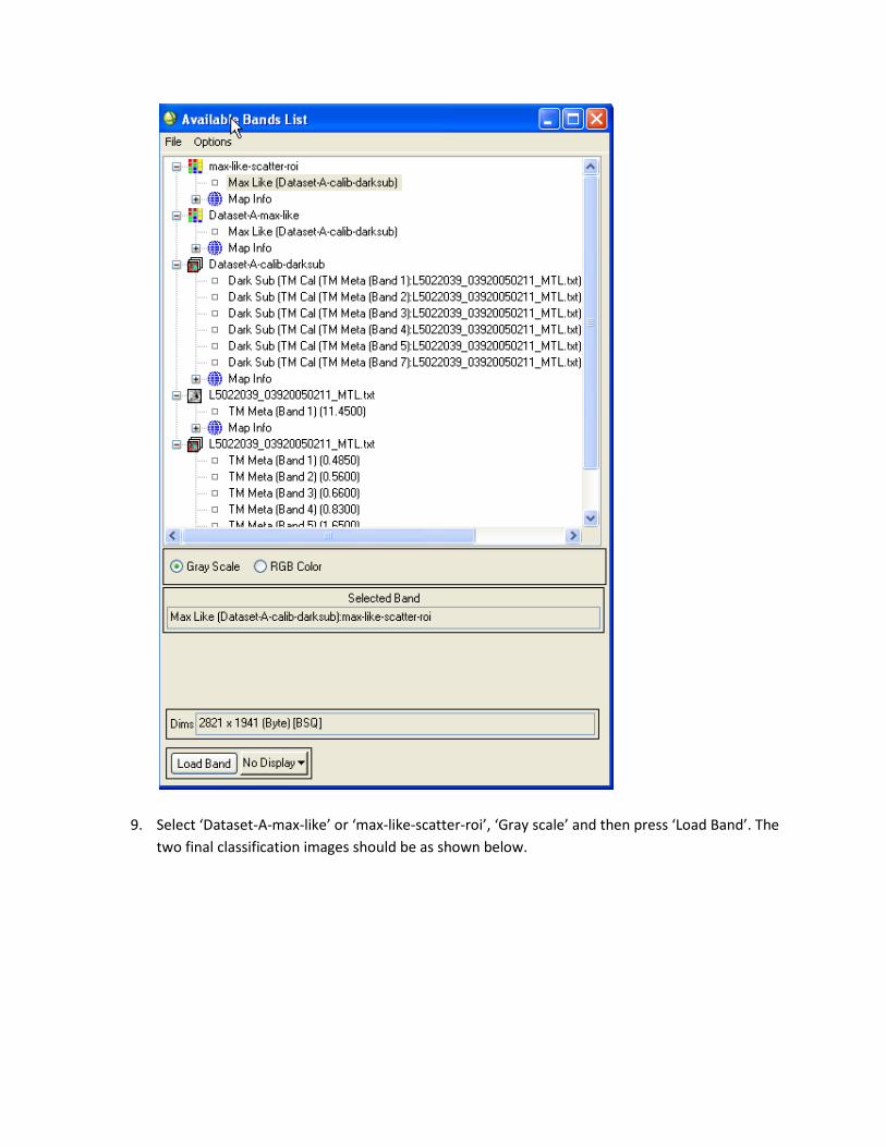
9. Select ‘Dataset-A-max-like’ or ‘max-like-scatter-roi’, ‘Gray scale’ and then press ‘Load Band’. The two final classification images should be as shown below.

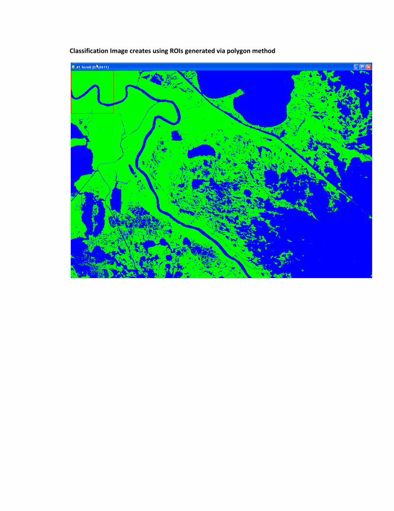
Classification Image creates using ROIs generated via polygon method

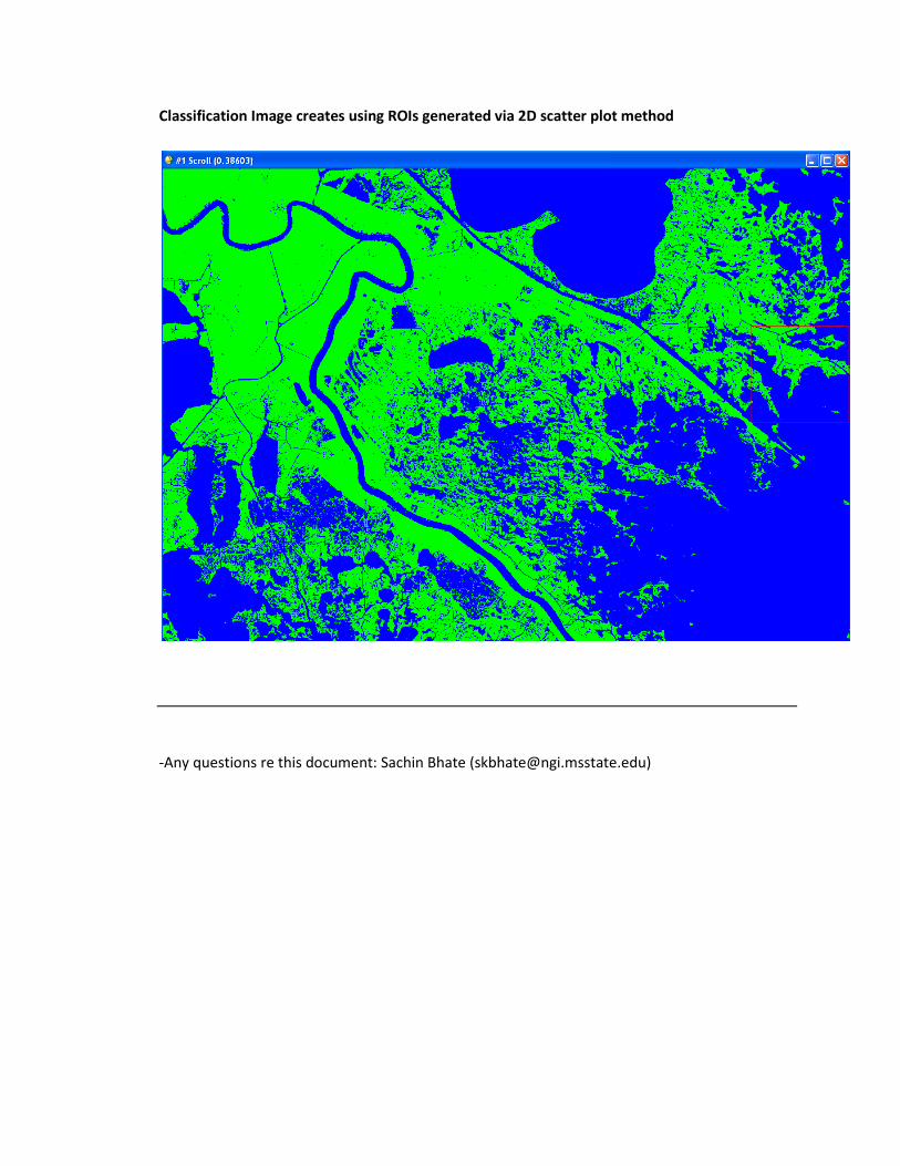
Classification Image creates using ROIs generated via 2D scatter plot method

-Any questions re this document: Sachin Bhate (skbhate@ngi.msstate.edu)