LANDSAT 8 (L8) DATA USERS HANDBOOK - WordPress.com · The Landsat 8 observatory offers these features: Data Continuity: Landsat 8 is the latest in a continuous series of land remote

LSDS-1574 Version 1.0

Department of the Interior U.S. Geological Survey

LANDSAT 8 (L8) DATA USERS HANDBOOK Version 1.0 June 2015 Any use of trade, firm, or product names is for descriptive purposes only and does not imply endorsement by the U.S. Government.

- ii - LSDS-1574 Version 1.0

LANDSAT 8 (L8)

DATA USERS HANDBOOK

June 2015

Approved By: ______________________________ K. Zanter Date LSDS CCB Chair USGS

EROS Sioux Falls, South Dakota

- iii - LSDS-1574 Version 1.0

Executive Summary

The Landsat 8 Data User’s Handbook is a living document prepared by the U.S. Geological Survey Landsat Project Science Office at the Earth Resources Observation and Science (EROS) Center in Sioux Falls, SD and the NASA Landsat Project Science Office at NASA's Goddard Space Flight Center in Greenbelt, Maryland. Its purpose is to provide a basic understanding and associated reference material for the Landsat 8 observatory and its science data products. In doing so, this document does not include a detailed description of all technical details of the Landsat 8 mission, but focuses on the information needed by the users to gain an understanding of the science data products. The Landsat 8 Data User’s Handbook includes various sections that provide an overview of reference material and a more detailed description of applicable data user and product information. This document describes the background for the Landsat 8 mission as well as previous Landsat missions (Section 1) before providing a comprehensive overview of the current Landsat 8 observatory, including the spacecraft, both the OLI and TIRS instruments and the Landsat 8 concept of operations (Section 2). The document then includes an overview of radiometric and geometric instrument calibration as well as a description of the observatory component reference systems and the calibration parameter file (Section 3), followed by a comprehensive description of Level 1 Products and product generation (Section 4). Addressed next is the conversion of DNS to physical units (Section 5) and finally, an overview of data search and access using the various on-line tools (Section 6). The applicable reference materials are included at the along with the list of known issues associated with Landsat 8 data (Appendix A) and an example of the Level-1 product metadata (Appendix B). This document is controlled by the LSDS Configuration Control Board (CCB). Please submit changes to this document, as well as supportive material justifying the proposed changes, via a Change Request (CR) to the Process and Change Management Tool.

- iv - LSDS-1574 Version 1.0

Document History

Document Number

Document Version

Publication Date

Change Number

LSDS-1574 Version 1.0 June 2015 CR 12286

- v - LSDS-1574 Version 1.0

Contents

Executive Summary ..................................................................................................... iii

Document History ........................................................................................................ iv

Contents ......................................................................................................................... v

List of Figures ............................................................................................................. vii

List of Tables .............................................................................................................. viii

Section 1 Introduction .............................................................................................. 1

1.1 Foreword ........................................................................................................... 1 1.2 Background ....................................................................................................... 2

1.2.1 Previous Missions ...................................................................................... 2 1.2.2 Operations & Management ........................................................................ 3

1.3 Landsat 8 Mission ............................................................................................. 4

1.3.1 Overall Mission Objectives ......................................................................... 4

1.3.2 System Capabilities ................................................................................... 4 1.3.3 Global Survey Mission ............................................................................... 5

1.3.4 Rapid Data Availability ............................................................................... 5 1.3.5 International Ground Stations .................................................................... 6

1.4 Document Purpose ........................................................................................... 6

1.5 Document Organization .................................................................................... 6 Section 2 Observatory Overview ............................................................................. 7

2.1 Concept of Operations ...................................................................................... 7 2.2 Operational Land Imager (OLI) ......................................................................... 8 2.3 Thermal Infrared Sensor (TIRS) ...................................................................... 12

2.4 Spacecraft Overview ....................................................................................... 14

2.4.1 Spacecraft Data Flow Operations ............................................................ 15 Section 3 Instrument Calibration ........................................................................... 17

3.1 Radiometric Characterization and Calibration Overview ................................. 17

3.1.1 Instrument Characterization and Calibration ............................................ 19 3.1.2 Pre-Launch .............................................................................................. 21

3.1.3 Post-Launch ............................................................................................. 23 3.1.4 Operational Radiometric Tasks ................................................................ 24

3.2 Geometric Calibration Overview ..................................................................... 26 3.2.1 Collection Types ...................................................................................... 29 3.2.2 Pre-Launch .............................................................................................. 29

3.2.3 OLI Geodetic Accuracy Assessment........................................................ 30

3.2.4 Sensor Alignment Calibration .................................................................. 31

3.2.5 Geometric Accuracy Assessment ............................................................ 31 3.2.6 OLI Internal Geometric Characterization and Calibration......................... 31 3.2.7 TIRS Internal Geometric Characterization and Calibration ...................... 33 3.2.8 OLI Spatial Performance Characterization ............................................... 34 3.2.9 OLI Bridge Target MTF Estimation .......................................................... 34 3.2.10 Geometric Calibration Data Requirements .............................................. 35

3.3 Calibration Parameters ................................................................................... 38

- vi - LSDS-1574 Version 1.0

3.3.1 Calibration Parameter File ....................................................................... 39

3.3.2 Bias Parameter Files................................................................................ 41 3.3.3 Response Linearization Lookup Table File .............................................. 42

Section 4 Level 1 Products .................................................................................... 43

4.1 Level 1 Product Generation ............................................................................ 43 4.1.1 Overview .................................................................................................. 43 4.1.2 Level 1 Processing System ...................................................................... 43 4.1.3 Ancillary Data ........................................................................................... 45

4.1.4 Data Products .......................................................................................... 46 4.1.5 Calculation of Scene Quality .................................................................... 55

4.2 Level 1 Product Description ............................................................................ 56 4.2.1 Science Data Content and Format ........................................................... 56 4.2.2 Metadata Content and Format ................................................................. 59

4.2.3 Quality Assurance Band .......................................................................... 59 Section 5 Conversion of DNs to Physical Units ................................................... 61

5.1 OLI and TIRS at Sensor Spectral Radiance.................................................... 61

5.2 OLI Top of Atmosphere Reflectance ............................................................... 61 5.3 TIRS Top of Atmosphere Brightness Temperature ......................................... 62 5.4 Unpacking Quality Assurance Band Bits ......................................................... 62

5.5 LandsatLook Quality Image (.png) .................................................................. 64 Section 6 Data Search and Access ....................................................................... 66

6.1 Earth Explorer (EE) ......................................................................................... 66 6.2 Global Visualization Viewer (GloVis) ............................................................... 69 6.3 LandsatLook Viewer ....................................................................................... 70

Appendix A Known Issues ..................................................................................... 72

A.1 TIRS Stray Light .............................................................................................. 72

A.2 Striping and Banding ....................................................................................... 75 A.3 SCA Overlaps ................................................................................................. 79

A.4 Oversaturation ................................................................................................ 80 A.5 Single Event Upsets ........................................................................................ 81

A.5.1 Observatory Component Reference Systems .......................................... 82

A.6 OLI Instrument Line-of-Sight (LOS) Coordinate System ................................. 82 A.7 TIRS Instrument Coordinate System .............................................................. 83 A.8 Spacecraft Coordinate System ....................................................................... 84 A.9 Navigation Reference Coordinate System ...................................................... 84 A.10 SIRU Coordinate System ................................................................................ 85

A.11 Orbital Coordinate System .............................................................................. 85

A.12 ECI J2000 Coordinate System ........................................................................ 86 A.13 ECEF Coordinate System ............................................................................... 87 A.14 Geodetic Coordinate System .......................................................................... 88

A.15 Map Projection Coordinate System ................................................................. 89 Appendix B Metadata File (MTL.txt) ...................................................................... 90

References ................................................................................................................... 95

- vii - LSDS-1574 Version 1.0

List of Figures

Figure 1-1. Continuity of Multispectral Data Coverage Provided by Landsat Missions ... 3 Figure 2-1. Illustration of Landsat 8 Observatory ............................................................ 7 Figure 2-2. OLI Instrument .............................................................................................. 8

Figure 2-3. OLI Signal-To-Noise (SNR) Performance at Ltypical .................................. 10 Figure 2-4. OLI Focal Plane .......................................................................................... 11 Figure 2-5. Odd/Even SCA Band Arrangement ............................................................. 11 Figure 2-6. TIRS Instrument with Earthshield Deployed................................................ 12 Figure 2-7. TIRS Focal Plane ........................................................................................ 13

Figure 2-8. TIRS Optical Sensor Unit ............................................................................ 14 Figure 3-1. Simulated OLI Image of the Lake Pontchartrain Causeway (left) and

Interstate-10 Bridge (right) Targets in WRS 022/039 ............................................. 35

Figure 4-1. LPGS Standard Product Data Flow ............................................................ 44 Figure 4-2. Level 1 Product Ground Swatch and Scene Size ....................................... 46 Figure 4-3. A Diagram of the First Pass ACCA Algorithm ............................................. 52

Figure 4-4. A Temperate Region Affected by Cirrus ..................................................... 54 Figure 4-5. Landsat 8 Spectral Bands and Wavelengths compared to Landsat 7 ETM+

............................................................................................................................... 57

Figure 4-6. Quality Band (BQA.TIF) displayed for Landsat 8 Sample Data (Path 45 Row 30) Acquired April 23, 2013 .................................................................................... 60

Figure 5-1. Landsat Look "Quality" Image (QA.png) displayed as .jpg for reference only Landsat 8 sample data Path 45 Row 30 Acquired April 23, 2013 .......................... 65

Figure 6-1. EarthExplorer Interface ............................................................................... 67

Figure 6-2. EarthExplorer Landsat Data Sets ................................................................ 67

Figure 6-3. EarthExplorer Results - Browse Image Display .......................................... 68 Figure 6-4. EarthExplorer Results Controls ................................................................... 68 Figure 6-5. Global Visualization Viewer (GloVis) Interface ............................................ 69

Figure 6-6. The LandsatLook Viewer ............................................................................ 70 Figure 6-7. Display of Landsat Imagery ......................................................................... 71

Figure 6-8. LandsatLook Viewer screen display. ........................................................... 71 Figure A-1. TIRS Image of Lake Superior Showing Apparent Time-Varying Errors ...... 73 Figure A-2. TIRS Special Lunar Scan to Characterize the Stray Light Issue ................. 74 Figure A-3. Thermal Band Errors (left group) Prior to Calibration Adjustment and (right

group) After Calibration Adjustment ....................................................................... 75 Figure A-4. Striping and Banding Observed in Band 1 (CA Band) ................................ 76 Figure A-5. Striping and Banding observed in Band 2 (Blue) ........................................ 77

Figure A-6. Striping and Banding observed in TIRS Band 10 ....................................... 78 Figure A-7. SCA Overlap Visible in Band 9 (Cirrus Band) ............................................. 79 Figure A-8. SCA Overlap Visible in TIRS Band 10 ........................................................ 80 Figure A-9. Oversaturation Example in OLI SWIR Bands 6 & 7 .................................... 81

Figure A-10. Example of SEU Event Measured by OLI – SEU Manifests as a Line of Single-Frame Bright Spots ..................................................................................... 82

Figure A-11. OLI Line-of-Sight Coordinate System ....................................................... 83

Figure A-12. TIRS Line-of-Sight Coordinates ................................................................ 84

- viii - LSDS-1574 Version 1.0

Figure A-13. Orbital Coordinate System ........................................................................ 86

Figure A-14. Earth-Centered Inertial (ECI) Coordinate System ..................................... 87 Figure A-15. Earth-Centered Earth Fixed (ECEF) Coordinate Systems ........................ 88

Figure A-16. Geodetic Coordinate System .................................................................... 89

List of Tables

Table 1-1. Comparison of Landsat 7 and Landsat 8 Observatory Capabilities ................ 5 Table 2-1. OLI and TIRS Spectral Bands Compared to ETM+ Spectral Bands .............. 9 Table 2-2. OLI Specified and Performance Signal-to-Noise (SNR) Ratios Compared to

ETM+ Performance ................................................................................................ 10 Table 2-4. TIRS Noise-Equivalent-Change-in Temperature (NEΔT) ............................. 13 Table 3-1. Summary of Calibration Activities, Their Purpose, and How Measurements

are Used in Building the Calibration Parameter Files ............................................. 19 Table 3-2. Summary of Geometric Characterization and Calibration Activities ............. 29 Table 4-1. Standard: Ls8ppprrrYYYYDDDGGGVV_FT.ext .......................................... 58

Table 4-2. Compressed: Ls8ppprrrYYYYDDDGGGVV.FT.ext ..................................... 58 Table 5-1. Bits Populated in the Level 1 QA Band ........................................................ 62 Table 5-2. A Summary of Some Regularly Occurring QA Bit Settings .......................... 64

Table 5-3. Bits and Colors Associated with LandsatLook Quality Image....................... 65 Table A-1. TIRS Band Variability ................................................................................... 75

- 1 - LSDS-1574 Version 1.0

Section 1 Introduction

1.1 Foreword

The Landsat Program has provided over 42 years of calibrated high spatial resolution data of the Earth's surface to a broad and varied user community, including agribusiness, global change researchers, academia, state and local governments, commercial users, national security agencies, the international community, decision-makers, and the general public. Landsat images provide information meeting the broad and diverse needs of business, science, education, government, and national security. The mission of the Landsat Program is to provide repetitive acquisition of moderate-resolution multispectral data of the Earth's surface on a global basis. Landsat represents the only source of global, calibrated, moderate spatial resolution measurements of the Earth's surface that are preserved in a national archive and freely available to the

public. The data from the Landsat spacecraft constitute the longest record of the Earth's continental surfaces as seen from space. It is a record unmatched in quality, detail, coverage, and value. The Landsat 8 observatory offers these features:

Data Continuity: Landsat 8 is the latest in a continuous series of land remote

sensing satellites that began in 1972.

Global Survey Mission: Landsat 8 data systematically builds and periodically

refreshes a global archive of sun-lit, substantially cloud-free images of the Earth's

landmass.

Free Standard Data Products: Landsat 8 data products are available through the

USGS EROS Center at no charge.

Radiometric and Geometric Calibration: Data from the two sensors, the

Operational Land Imager (OLI) and the Thermal Infrared Sensor (TIRS), are

calibrated to better than 5% uncertainty in terms of top-of-atmosphere reflectance

or absolute spectral radiance, and having an absolute geodetic accuracy better

than 65 meters circular error at 90% confidence (CE 90).

Responsive Delivery: Automated request processing systems provide products

electronically within 48 hours of order (nominally much faster).

The continuation of the Landsat Program is an integral component of the U.S. Global Change Research Program and will be used to address a number of science priorities, such as land cover change and land use dynamics. Landsat 8 is part of a global


research program known as NASA’s Science Mission Directorate, a long-term program that is studying changes in Earth's global environment. In the Landsat Program tradition, Landsat 8 continues to provide critical information to those who characterize, monitor, manage, explore, and observe the land surfaces of Earth over time. The U.S. Geological Survey has a long history as a national leader in land cover and land use mapping and monitoring. Landsat data, including Landsat 8 and archive holdings, are essential for USGS efforts to document the rates and causes of land cover and land use change, and to address the linkages between land cover and use dynamics on water quality and quantity, biodiversity, energy development, and many other environmental topics. In addition, the USGS is working toward the provision of long-term environmental records that describe ecosystem disturbances and conditions.

1.2 Background

The Land Remote Sensing Policy Act of 1992 (U.S. Code Title 15, Chapter 82) directed the federal agencies involved in the Landsat program to study options for a successor mission to Landsat 7, ultimately launched in 1999 with a five-year design life, that maintained data continuity with the Landsat system. The Act further expressed a preference for the development of this successor system by the private sector as long as such a development met the goals of data continuity. The Landsat 8 project suffered several setbacks in its attempt to meet these data continuity goals. Beginning in 2002, three distinct acquisition and implementation strategies were pursued: (1) purchase of observatory imagery from a commercially owned and operated satellite system partner (commonly referred to as a government “data buy”), (2) flying a Landsat instrument on NOAA’s NPOESS series of satellites, and (3) finally selection of a “free-flying” Landsat satellite. Considerable delays to Landsat 8 implementation were incurred as a result. The matter wasn’t resolved until 2007 when it was determined that NASA would procure the next mission space segment and the USGS would develop the ground system and operate the mission after launch. The basic Landsat 8 requirements remained consistent through this extended strategic formulation phase of mission development. The 1992 Land Remote Sensing Policy Act (U.S. Code Title 15, Chapter 82) established data continuity as a fundamental goal and defined continuity as providing data “sufficiently consistent (in terms of acquisition geometry, coverage characteristics, and spectral characteristics) with previous Landsat data to allow comparisons for global and regional change detection and characterization.” This direction has provided the guiding principal for specifying Landsat 8 requirements from the beginning with the most recently launched Landsat satellite, Landsat 7, serving as a technical minimum standard for system performance and data quality.

1.2.1 Previous Missions

Landsat satellites have been providing multispectral images of the Earth continuously since the early 1970's. A unique 42+ year data record of the Earth's land surface now exists. This unique retrospective portrait of the Earth's surface has been used across


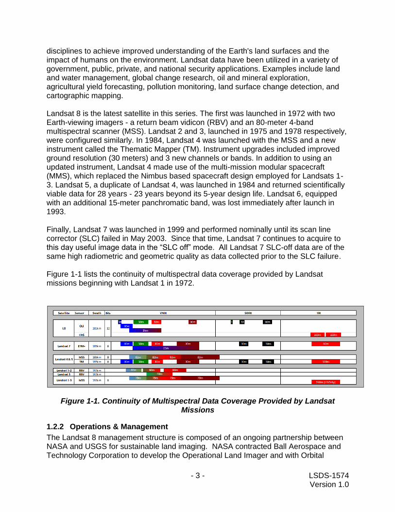
disciplines to achieve improved understanding of the Earth's land surfaces and the impact of humans on the environment. Landsat data have been utilized in a variety of government, public, private, and national security applications. Examples include land and water management, global change research, oil and mineral exploration, agricultural yield forecasting, pollution monitoring, land surface change detection, and cartographic mapping. Landsat 8 is the latest satellite in this series. The first was launched in 1972 with two Earth-viewing imagers - a return beam vidicon (RBV) and an 80-meter 4-band multispectral scanner (MSS). Landsat 2 and 3, launched in 1975 and 1978 respectively, were configured similarly. In 1984, Landsat 4 was launched with the MSS and a new instrument called the Thematic Mapper (TM). Instrument upgrades included improved ground resolution (30 meters) and 3 new channels or bands. In addition to using an updated instrument, Landsat 4 made use of the multi-mission modular spacecraft (MMS), which replaced the Nimbus based spacecraft design employed for Landsats 1-3. Landsat 5, a duplicate of Landsat 4, was launched in 1984 and returned scientifically viable data for 28 years - 23 years beyond its 5-year design life. Landsat 6, equipped with an additional 15-meter panchromatic band, was lost immediately after launch in 1993. Finally, Landsat 7 was launched in 1999 and performed nominally until its scan line corrector (SLC) failed in May 2003. Since that time, Landsat 7 continues to acquire to this day useful image data in the “SLC off” mode. All Landsat 7 SLC-off data are of the same high radiometric and geometric quality as data collected prior to the SLC failure. Figure 1-1 lists the continuity of multispectral data coverage provided by Landsat missions beginning with Landsat 1 in 1972.

Figure 1-1. Continuity of Multispectral Data Coverage Provided by Landsat Missions

1.2.2 Operations & Management

The Landsat 8 management structure is composed of an ongoing partnership between NASA and USGS for sustainable land imaging. NASA contracted Ball Aerospace and Technology Corporation to develop the Operational Land Imager and with Orbital


Sciences Corporation to build the spacecraft. The Thermal Infrared Sensor was built by NASA Goddard Space Flight Center. NASA was also responsible for the satellite launch and completion of a 90-day on-orbit check out before handing operations to the USGS. The USGS was responsible for the development of the ground system and is responsible for operation and maintenance of the observatory and the ground system for the life of the mission. In this role, the USGS captures, processes, and distributes Landsat 8 data and is responsible for maintaining the Landsat 8 data archive. The Landsat Project at the USGS Earth Resources Observation and Science (EROS) Center manages the overall Landsat 8 Mission Operations. In this capacity, USGS EROS directs on-orbit flight operations, implements mission policies, directs acquisition strategy, and interacts with International Ground Stations. USGS EROS captures Landsat 8 data and performs pre-processing, archiving, product generation, and distribution functions. USGS EROS also provides a public interface into the archive for data search and ordering.

1.3 Landsat 8 Mission

The Landsat 8 mission objective is to provide timely, high quality visible and infrared images of all landmass and near-coastal areas on the Earth, continually refreshing an existing Landsat database. Data input into the system is sufficiently consistent with currently archived data in terms of acquisition geometry, calibration, coverage and spectral characteristics to allow for comparison of global and regional change detection and characterization.

1.3.1 Overall Mission Objectives

Landsat 8 has a design lifetime of five years and carries 10 years of fuel consumables. The overall objectives of the Landsat 8 mission are:

Provide data continuity with Landsats 4, 5, and 7.

Offer 16-day repetitive Earth coverage, an 8-day repeat with a Landsat 7 offset.

Build and periodically refresh a global archive of sun-lit, substantially cloud-free,

land images.

1.3.2 System Capabilities

The Landsat 8 system is robust, high performing, and of extremely high data quality. System capabilities include:

Provides for a systematic collection of global, high resolution, multispectral data.

Provides for a high volume of data collection. Unlike previous missions, Landsat 8 far surpasses the average collection of 400 scenes per day. Landsat 8 routinely surpasses 650 scenes per day imaged and collected in the USGS archive.

Uses cloud cover predicts to avoid acquiring less useful data.

Ensures all data imaged are collected by a U.S. ground station.


The Landsat 8 observatory offers many improvements over its predecessor, Landsat 7. See Table 1-1 for a high level comparison of Landsat 7 and Landsat 8 observatory capabilities. These will be discussed further in the following sections.

Table 1-1. Comparison of Landsat 7 and Landsat 8 Observatory Capabilities

1.3.3 Global Survey Mission

An important operational strategy of the Landsat 8 mission is to establish and maintain a global survey data archive. Landsat 8 follows the same "Worldwide Reference System" used for Landsats 4, 5, and 7 bringing the entire world within view of its sensors once every 16 days. Also, similar to Landsat 7, Landsat 8 operations endeavor to systematically capture sun-lit, substantially cloud-free images of the Earth’s entire land surface. Initially developed for Landsat 7, the Long Term Acquisition Plan (LTAP) for Landsat 8 defines the acquisition pattern for the mission in order to create and update the global archive to ensure global continuity.

1.3.4 Rapid Data Availability

Landsat 8 data are downlinked and processed into standard products within 24 hours of acquisition. Level 0R, Level 1Gt, Level 1T, and LandsatLook products are available through the User Portal. All users are required to register through Earth Explorer at http://earthexplorer.usgs.gov. All products are accessible via the internet for download via HTTP; there are no product media options. As with all Landsat data, products are available at no cost to the user. Available data can be viewed through a number of interfaces:

1. Earth Explorer: http://earthexplorere.usgs.gov

2. Global Visualization Viewer: http://glovis.usgs.gov

3. LandsatLook Viewer: http://landsatlook.usgs.gov

Scenes/Day

SSR Size

Sensor Type

Compression

Image D/L

Data Rate

Encoding

Ranging

Orbit

Crossing Time ~ 10:00 AM ~ 10:11 AM

L7 L8

not fully CCSDS compliant CCSDS, LDPC FEC

S-Band 2-Way Doppler GPS

705 Km Sun-Sync 98.2° inclination (WRS2) 705 Km Sun-Sync 98.2° inclination (WRS2)

No ~2:1 Variable Rice Compression

X-Band GXA×3 X-Band Earth Coverage

150 Mbits/sec × 3 Channels/Frequencies 384 Mbits/sec, CCSDS Virtual Channels

~450 ~650

378 Gbits, block-based 3.14 Terabit, file-based

ETM+, Whisk-Broom Pushbroom (both OLI and TIRS)

http://earthexplorer.usgs.gov/

http://earthexplorere.usgs.gov/

http://glovis.usgs.gov/

http://landsatlook.usgs.gov/


1.3.5 International Ground Stations

Landsat has worked cooperatively with international ground stations for decades. For the first time in the history of the Landsat mission, all data downlinked to international ground stations are written to the Solid State Recorder and downlinked to USGS EROS for inclusion in the USGS Landsat archive. There are no unique data held at international ground stations. Updated information and a map displaying international ground stations can be found at: http://landsat.usgs.gov/about_ground_stations.php.

1.4 Document Purpose

The Landsat 8 Data Users Handbook is a living document prepared by the U.S. Geological Survey Landsat Project Science Office at the Earth Resources Observation and Science (EROS) Center in Sioux Falls, SD and the NASA Landsat Project Science Office at NASA's Goddard Space Flight Center in Greenbelt, Maryland. Its purpose is to provide a basic understanding and associated reference material for the Landsat 8 observatory and its science data products.

1.5 Document Organization

This document contains the following sections:

Section 1 provides a Landsat program foreword and introduction

Section 2 provides an overview of the Landsat 8 observatory

Section 3 provides an overview of instrument calibration

Section 4 discusses Level 1 Products

Section 5 addresses the conversion of product DNs to physical units

Section 6 identifies data search and access portals

Appendix A addresses known issues associated with Landsat 8 data

Appendix B displays the metadata file.

The References section contains a list of applicable documents

http://landsat.usgs.gov/about_ground_stations.php


Section 2 Observatory Overview

The Landsat 8 observatory is designed for a 705 km, sun-synchronous orbit, with a 16-day repeat cycle, completely orbiting the Earth every 98.9 minutes. S-Band is used for commanding and housekeeping telemetry operations while X-Band is used for instrument data downlink. A 3.14 terabit Solid State Recorder (SSR) brings back an unprecedented number of images to the USGS EROS Center archive. Landsat 8 carries a two-sensor payload: the Operational Land Imager (OLI), built by the Ball Aerospace & Technologies Corporation; and the Thermal Infrared Sensor (TIRS), built by the NASA Goddard Space Flight Center (GSFC). Both the OLI and TIRS sensors simultaneously image every scene, but are capable of independent use should a problem in either sensor arise. In normal operation the sensors view the Earth at nadir on the sun synchronous WRS-2 orbital path, but special collections may be scheduled off-nadir. Both sensors offer technical advancements over earlier Landsat instruments. The spacecraft with its two integrated sensors is referred to as the Landsat 8 observatory.

2.1 Concept of Operations

The fundamental Landsat 8 operations concept is to collect, archive, process, and distribute science data in a manner consistent with the operation of the Landsat 7 satellite system. To that end, the Landsat 8 observatory operates in a near-circular, near-polar, sun-synchronous orbit with a 705 km altitude at the equator. The observatory has a 16-day ground track repeat cycle with an equatorial crossing at 10:11 a.m. (+/−15 min) mean local time during the descending node. In this orbit, the Landsat 8 observatory follows a sequence of fixed ground tracks (also known as paths) defined by the second Worldwide Reference System (WRS-2). WRS-2 is a path/row coordinate system used to catalog all the science image data acquired from the Landsat 4 - 8 satellites. The Landsat 8 launch and initial orbit adjustments placed the observatory in an orbit to ensure an eight-day offset between Landsat 7 and Landsat 8 coverage of each WRS-2 path. The Mission Operation Center (MOC) sends commands to the satellite once every 24 hours via S-band communications from the ground system to schedule daily data collections. A Long Term Acquisition Plan (LTAP-8) sets priorities for collecting data along the WRS-2 ground paths covered in a particular 24-hour period. LTAP-8 is

OLI

TIRS

Spacecraft Bus Solar

Panel

Figure 2-1. Illustration of Landsat 8 Observatory


modeled on the systematic data acquisition plan developed for Landsat 7 (Arvidson et al., 2006). OLI and TIRS collect data jointly to provide coincident images of the same surface areas. The MOC nominally schedules the collection of 400 OLI and TIRS scenes per day where each scene covers a 190-by-180 km surface area. The objective of scheduling and data collection is to provide near cloud-free coverage of the global landmass for each season of the year. Since the 2014 growing season, however, the Landsat 8 mission has been routinely acquiring approximately 725 scenes/day. The Landsat 8 observatory initially stores OLI and TIRS data on board in a solid-state recorder. The MOC commands the observatory to transmit the stored data to the ground via an X-band data stream from an all-earth omni antenna. The Landsat 8 ground network receives the data at several stations and these stations forward the data to the EROS Center. The ground network includes international stations operated under the sponsorship of foreign governments referred to as International Cooperators (ICs). Data management and distribution by the ICs is in accordance with bilateral agreements between each IC and the U.S. Government. The data received from the ground network are stored and archived at the EROS Center where also Landsat 8 data products are generated. The OLI and TIRS data for each WRS-2 scene are merged to create a single product containing the data from both sensors. The data from both sensors are radiometrically corrected and co-registered to a cartographic projection with corrections for terrain displacement resulting in a standard orthorectified digital image called the Level 1T product. The interface to the Landsat 8 data archive is called the User Portal and it allows anyone to search the archive, view browse images, and request data products that are distributed electronically through the internet at no charge (see Section 6).

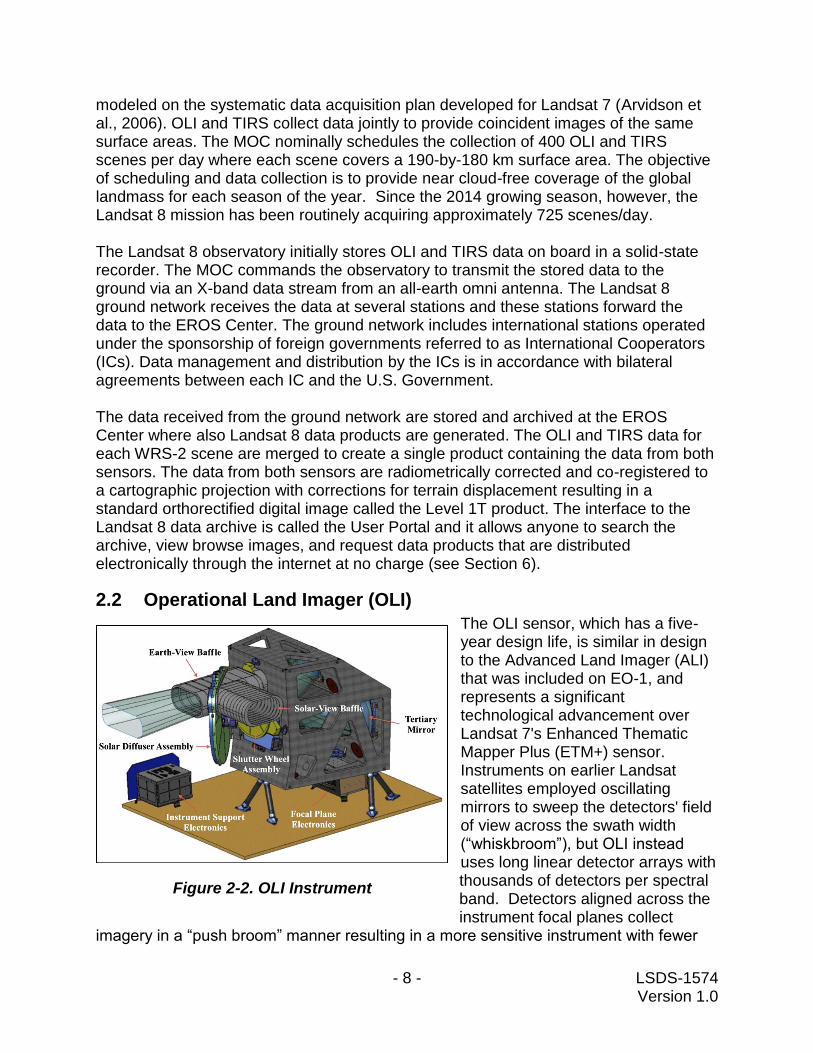
2.2 Operational Land Imager (OLI)

The OLI sensor, which has a five-year design life, is similar in design to the Advanced Land Imager (ALI) that was included on EO-1, and represents a significant technological advancement over Landsat 7's Enhanced Thematic Mapper Plus (ETM+) sensor. Instruments on earlier Landsat satellites employed oscillating mirrors to sweep the detectors' field of view across the swath width (“whiskbroom”), but OLI instead uses long linear detector arrays with thousands of detectors per spectral band. Detectors aligned across the instrument focal planes collect

imagery in a “push broom” manner resulting in a more sensitive instrument with fewer

Figure 2-2. OLI Instrument


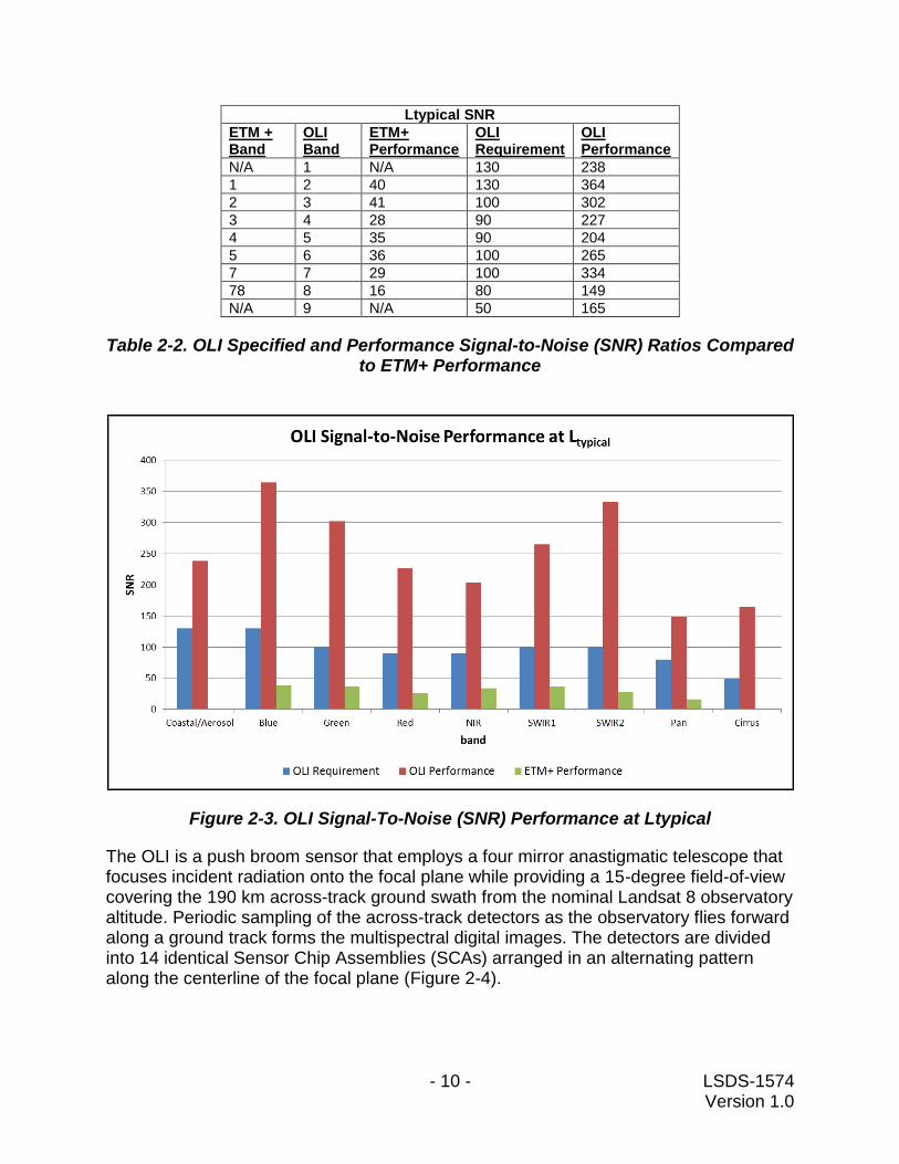
moving parts. OLI has a four-mirror telescope and data generated by OLI are quantized to 12 bits, compared to the 8-bit data produced by the TM & ETM+ sensor. The OLI sensor collects image data for nine shortwave spectral bands over a 190 km swath with a 30 m spatial resolution for all bands except the 15 m panchromatic band. The widths of several OLI bands are refined to avoid atmospheric absorption features within ETM+ bands. The biggest change occurs in OLI band 5 (0.845–0.885 μm) to exclude a water vapor absorption feature at 0.825 μm in the middle of the ETM+ near infrared band (band 4; 0.775–0.900 μm). The OLI panchromatic band, band 8, is also narrower relative to the ETM+ panchromatic band to create greater contrast between vegetated areas and land without vegetation cover. OLI also has two new bands in addition to the legacy Landsat bands (1-5, 7, and Pan). The Coastal /Aerosol band (band 1; 0.435-0.451 μm), principally for ocean color observations, is similar to ALI's band 1', and the new Cirrus band (band 9; 1.36-1.38 μm) aids in detection of thin clouds comprised of ice crystals (cirrus clouds will appear bright while most land surfaces will appear dark through an otherwise cloud-free atmospheres containing water vapor). OLI has stringent radiometric performance requirements and is required to produce data calibrated to an uncertainty of less than 5% in terms of absolute, at-aperture spectral radiance and to an uncertainty of less than 3% in terms of top-of-atmosphere spectral reflectance for each of the spectral bands in Table 2-1. These values are comparable to the uncertainties achieved by ETM+ calibration. The OLI signal-to-noise ratio (SNR) specifications, however, were set higher than ETM+ performance based on results from the ALI. Table 2-2 and Figure 2-3 show the OLI specifications and performance compared to ETM+ performance for signal-to-noise ratios at specified levels of typical spectral radiance (Ltypical) for each spectral band.

Table 2-1. OLI and TIRS Spectral Bands Compared to ETM+ Spectral Bands

- 10 - LSDS-1574 Version 1.0

Ltypical SNR

ETM + Band

OLI Band

ETM+ Performance

OLI Requirement

OLI Performance

N/A 1 N/A 130 238

1 2 40 130 364

2 3 41 100 302

3 4 28 90 227

4 5 35 90 204

5 6 36 100 265

7 7 29 100 334

78 8 16 80 149

N/A 9 N/A 50 165

Table 2-2. OLI Specified and Performance Signal-to-Noise (SNR) Ratios Compared to ETM+ Performance

Figure 2-3. OLI Signal-To-Noise (SNR) Performance at Ltypical

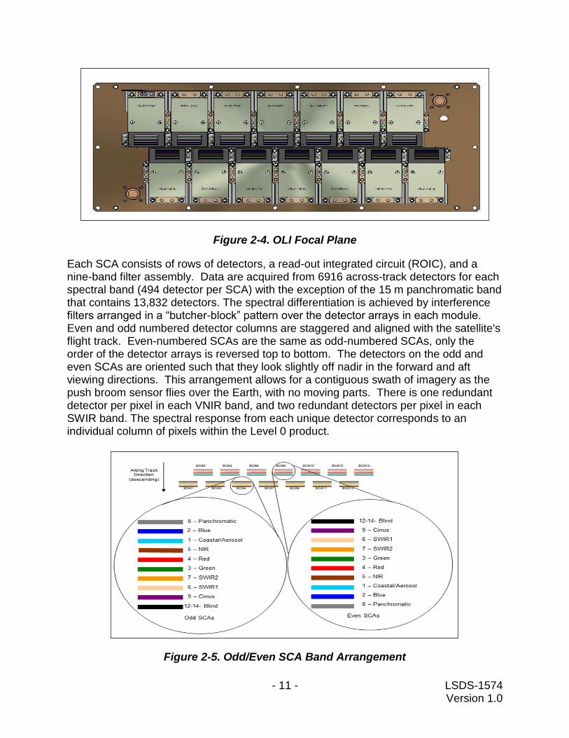
The OLI is a push broom sensor that employs a four mirror anastigmatic telescope that focuses incident radiation onto the focal plane while providing a 15-degree field-of-view covering the 190 km across-track ground swath from the nominal Landsat 8 observatory altitude. Periodic sampling of the across-track detectors as the observatory flies forward along a ground track forms the multispectral digital images. The detectors are divided into 14 identical Sensor Chip Assemblies (SCAs) arranged in an alternating pattern along the centerline of the focal plane (Figure 2-4).

- 11 - LSDS-1574 Version 1.0

Figure 2-4. OLI Focal Plane

Each SCA consists of rows of detectors, a read-out integrated circuit (ROIC), and a nine-band filter assembly. Data are acquired from 6916 across-track detectors for each spectral band (494 detector per SCA) with the exception of the 15 m panchromatic band that contains 13,832 detectors. The spectral differentiation is achieved by interference filters arranged in a “butcher-block” pattern over the detector arrays in each module. Even and odd numbered detector columns are staggered and aligned with the satellite's flight track. Even-numbered SCAs are the same as odd-numbered SCAs, only the order of the detector arrays is reversed top to bottom. The detectors on the odd and even SCAs are oriented such that they look slightly off nadir in the forward and aft viewing directions. This arrangement allows for a contiguous swath of imagery as the push broom sensor flies over the Earth, with no moving parts. There is one redundant detector per pixel in each VNIR band, and two redundant detectors per pixel in each SWIR band. The spectral response from each unique detector corresponds to an individual column of pixels within the Level 0 product.

Figure 2-5. Odd/Even SCA Band Arrangement

- 12 - LSDS-1574 Version 1.0

Silicon PIN (SiPIN) detectors collect the data for the visible and near-infrared spectral bands (Bands 1 to 4 and 8) while Mercury–Cadmium–Telluride (MgCdTe) detectors are used for the shortwave infrared bands (Bands 6, 7, and 9). There is an additional 'blind' band that is shielded from incoming light and used to track small electronic drifts. There are 494 illuminated detectors per SCA, per band (988 for the PAN band); that is a total of 70,672 operating detectors that must be characterized and calibrated during nominal operations.

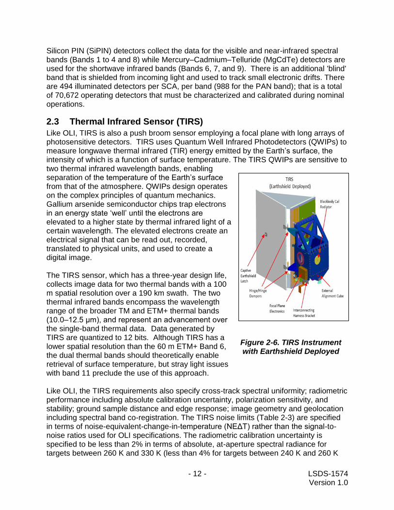
2.3 Thermal Infrared Sensor (TIRS)

Like OLI, TIRS is also a push broom sensor employing a focal plane with long arrays of photosensitive detectors. TIRS uses Quantum Well Infrared Photodetectors (QWIPs) to measure longwave thermal infrared (TIR) energy emitted by the Earth’s surface, the intensity of which is a function of surface temperature. The TIRS QWIPs are sensitive to two thermal infrared wavelength bands, enabling separation of the temperature of the Earth’s surface from that of the atmosphere. QWIPs design operates on the complex principles of quantum mechanics. Gallium arsenide semiconductor chips trap electrons in an energy state ‘well’ until the electrons are elevated to a higher state by thermal infrared light of a certain wavelength. The elevated electrons create an electrical signal that can be read out, recorded, translated to physical units, and used to create a digital image. The TIRS sensor, which has a three-year design life, collects image data for two thermal bands with a 100 m spatial resolution over a 190 km swath. The two thermal infrared bands encompass the wavelength range of the broader TM and ETM+ thermal bands (10.0–12.5 μm), and represent an advancement over the single-band thermal data. Data generated by TIRS are quantized to 12 bits. Although TIRS has a lower spatial resolution than the 60 m ETM+ Band 6, the dual thermal bands should theoretically enable retrieval of surface temperature, but stray light issues with band 11 preclude the use of this approach. Like OLI, the TIRS requirements also specify cross-track spectral uniformity; radiometric performance including absolute calibration uncertainty, polarization sensitivity, and stability; ground sample distance and edge response; image geometry and geolocation including spectral band co-registration. The TIRS noise limits (Table 2-3) are specified in terms of noise-equivalent-change-in-temperature (NEΔT) rather than the signal-to-noise ratios used for OLI specifications. The radiometric calibration uncertainty is specified to be less than 2% in terms of absolute, at-aperture spectral radiance for targets between 260 K and 330 K (less than 4% for targets between 240 K and 260 K

Figure 2-6. TIRS Instrument with Earthshield Deployed

- 13 - LSDS-1574 Version 1.0

and for targets between 330 K and 360 K), which is much lower than ETM+ measurements between 272 K and 285 K. Currently the performance of TIRS band 11 is slightly out of specification because of stray light entering the optical path.

TIRS Noise-Equivalent-Change-in-Temperature (NEΔT)

Band NEDT@240 NEDT@280 NEDT@320 NEDT@360

TIRS 10 0.069 0.053 0.046 0.043

TIRS 11 0.079 0.059 0.049 0.045

ETM+ 0.22

Table 2-3. TIRS Noise-Equivalent-Change-in Temperature (NEΔT)

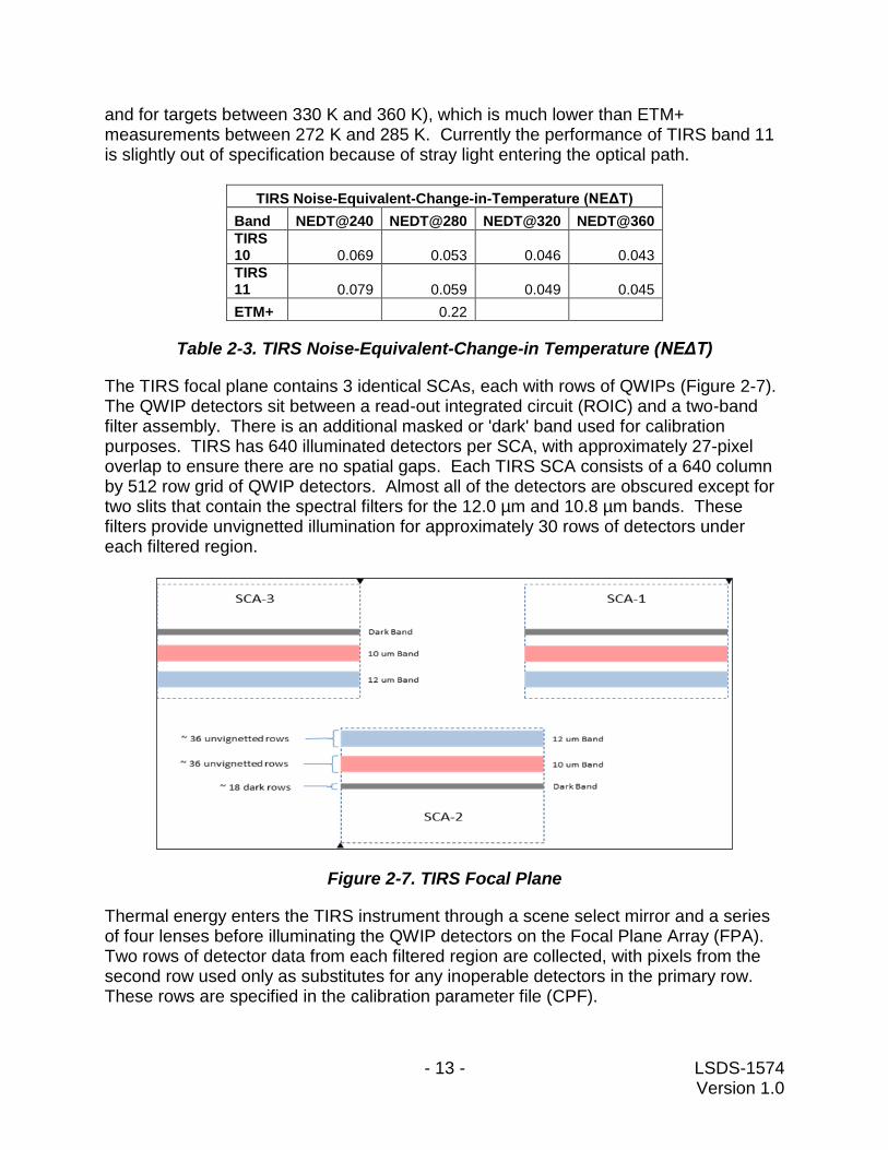
The TIRS focal plane contains 3 identical SCAs, each with rows of QWIPs (Figure 2-7). The QWIP detectors sit between a read-out integrated circuit (ROIC) and a two-band filter assembly. There is an additional masked or 'dark' band used for calibration purposes. TIRS has 640 illuminated detectors per SCA, with approximately 27-pixel overlap to ensure there are no spatial gaps. Each TIRS SCA consists of a 640 column by 512 row grid of QWIP detectors. Almost all of the detectors are obscured except for two slits that contain the spectral filters for the 12.0 µm and 10.8 µm bands. These filters provide unvignetted illumination for approximately 30 rows of detectors under each filtered region.

Figure 2-7. TIRS Focal Plane

Thermal energy enters the TIRS instrument through a scene select mirror and a series of four lenses before illuminating the QWIP detectors on the Focal Plane Array (FPA). Two rows of detector data from each filtered region are collected, with pixels from the second row used only as substitutes for any inoperable detectors in the primary row. These rows are specified in the calibration parameter file (CPF).

- 14 - LSDS-1574 Version 1.0

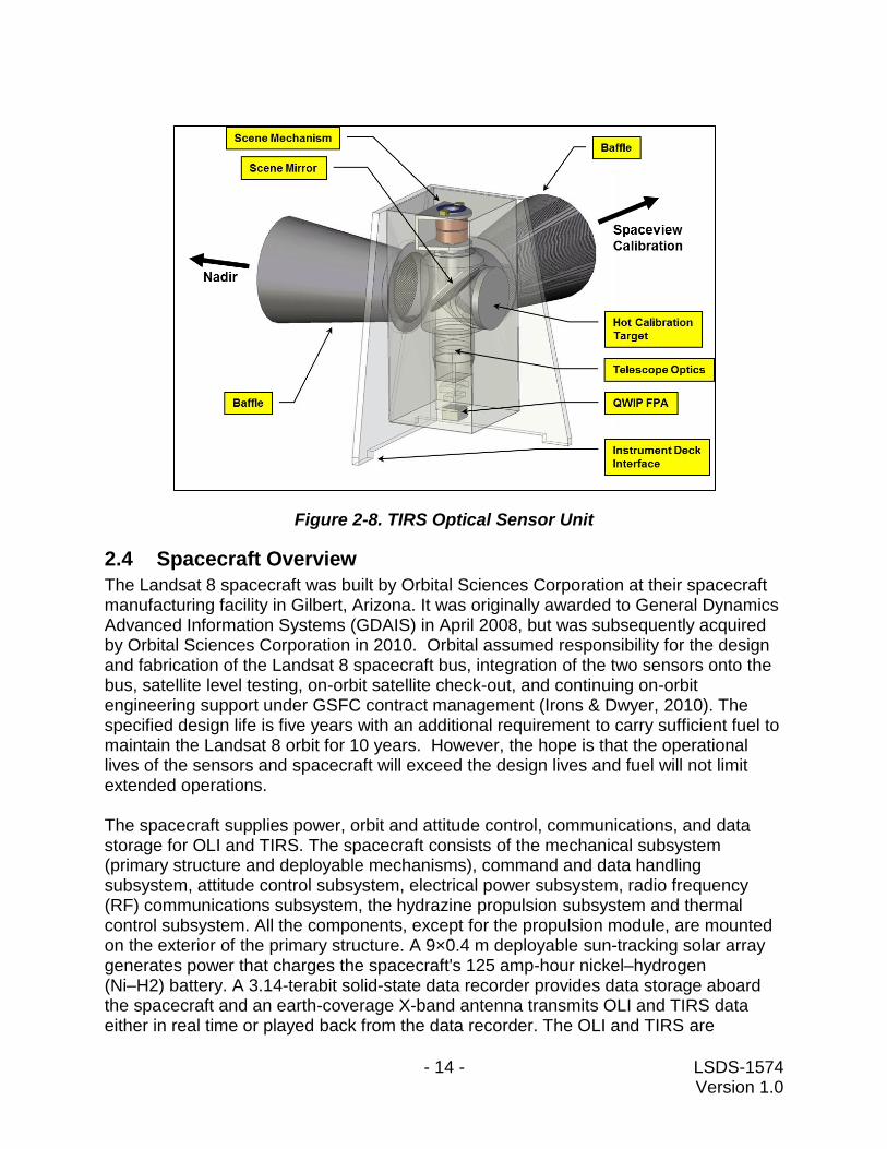
Figure 2-8. TIRS Optical Sensor Unit

2.4 Spacecraft Overview

The Landsat 8 spacecraft was built by Orbital Sciences Corporation at their spacecraft manufacturing facility in Gilbert, Arizona. It was originally awarded to General Dynamics Advanced Information Systems (GDAIS) in April 2008, but was subsequently acquired by Orbital Sciences Corporation in 2010. Orbital assumed responsibility for the design and fabrication of the Landsat 8 spacecraft bus, integration of the two sensors onto the bus, satellite level testing, on-orbit satellite check-out, and continuing on-orbit engineering support under GSFC contract management (Irons & Dwyer, 2010). The specified design life is five years with an additional requirement to carry sufficient fuel to maintain the Landsat 8 orbit for 10 years. However, the hope is that the operational lives of the sensors and spacecraft will exceed the design lives and fuel will not limit extended operations. The spacecraft supplies power, orbit and attitude control, communications, and data storage for OLI and TIRS. The spacecraft consists of the mechanical subsystem (primary structure and deployable mechanisms), command and data handling subsystem, attitude control subsystem, electrical power subsystem, radio frequency (RF) communications subsystem, the hydrazine propulsion subsystem and thermal control subsystem. All the components, except for the propulsion module, are mounted on the exterior of the primary structure. A 9×0.4 m deployable sun-tracking solar array generates power that charges the spacecraft's 125 amp-hour nickel–hydrogen (Ni–H2) battery. A 3.14-terabit solid-state data recorder provides data storage aboard the spacecraft and an earth-coverage X-band antenna transmits OLI and TIRS data either in real time or played back from the data recorder. The OLI and TIRS are

- 15 - LSDS-1574 Version 1.0

mounted on an optical bench at the forward end of the spacecraft. Fully assembled, the spacecraft without the instruments is approximately 3 m high and 2.4×2.4 m across with a mass of 2071 kg fully loaded with fuel.

2.4.1 Spacecraft Data Flow Operations

The Landsat 8 observatory receives a daily load of software commands transmitted from the ground. These command loads tell the observatory when to capture, store, and transmit image data from the OLI and TIRS. The daily command load covers the subsequent 72 hours of operations with the commands for the overlapping 48 hours overwritten each day. This precaution is taken to ensure that sensor and spacecraft operations continue in the event of a one or two day failure to successfully transmit or receive commands. The observatory's Payload Interface Electronics (PIE) ensures that image intervals are captured in accordance with the daily command loads. The OLI and TIRS are powered on continuously during nominal operations to maintain the thermal balance of the two instruments. The two sensors' detectors continuously produce signals that are digitized and sent to the PIE at an average rate of 265 megabits per second (Mbps) for the OLI and 26.2 Mbps for TIRS. Ancillary data such as sensor and select spacecraft housekeeping telemetry, calibration data, and other data necessary for image processing are also sent to the PIE. The PIE receives the OLI, TIRS, and ancillary data, merges these data into a mission data stream, identifies the mission data intervals scheduled for collection, performs a lossless compression of the OLI data (TIRS data are not compressed) using the Rice algorithm (Rice et al., 1993), and then sends the compressed OLI data and the uncompressed TIRS data to the 3.14 terabit SSR. The PIE also identifies those image intervals scheduled for real time transmission and sends those data directly to the observatory's X-band transmitter. The International Cooperator receiving stations only receive real time transmissions and the PIE also sends a copy of these data to the on-board SSR for playback and transmission to the Landsat 8 GNE receiving stations (USGS captures all of the data transmitted to International Cooperators). Recall that OLI and TIRS collect data coincidently and therefore the mission data streams from the PIE contain both OLI and TIRS data as well as ancillary data. The observatory broadcasts mission data files from its X-band, Earth-coverage antenna. The transmitter sends data to the antenna on multiple virtual channels providing for a total data rate of 384 Mbps. The observatory transmits real time data, SSR playback data, or both real-time data and SSR data depending on the time of day and the ground stations within view of the satellite. Transmissions from the Earth coverage antenna allow a ground station to receive mission data as long as the observatory is within view of the station antenna. OLI and TIRS collect the Landsat 8 science data. The spacecraft bus stores the OLI and TIRS data on an onboard solid-state recorder and then transmits the data to ground receiving stations. The ground system provides the capabilities necessary for planning and scheduling the operations of the Landsat 8 observatory and the capabilities necessary to manage the science data following transmission from the spacecraft. The real-time command and

- 16 - LSDS-1574 Version 1.0

control sub-system for observatory operations is known as the Mission Operations Element (MOE). A primary and back-up Mission Operations Center (MOC) houses the MOE with the primary MOC residing at NASA GSFC. The Data Processing and Archiving System (DPAS) at the EROS Center ingests, processes, and archives all Landsat 8 science and mission data returned from the observatory. The DPAS also provides a public interface to allow users to search for and receive data products over the internet (see Section 6).

- 17 - LSDS-1574 Version 1.0

Section 3 Instrument Calibration

3.1 Radiometric Characterization and Calibration Overview

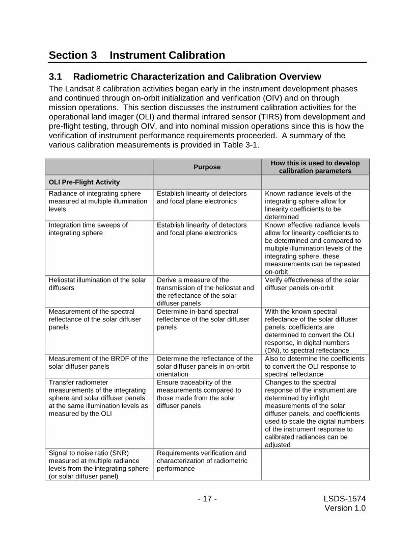
The Landsat 8 calibration activities began early in the instrument development phases and continued through on-orbit initialization and verification (OIV) and on through mission operations. This section discusses the instrument calibration activities for the operational land imager (OLI) and thermal infrared sensor (TIRS) from development and pre-flight testing, through OIV, and into nominal mission operations since this is how the verification of instrument performance requirements proceeded. A summary of the various calibration measurements is provided in Table 3-1.

Purpose How this is used to develop

calibration parameters

OLI Pre-Flight Activity

Radiance of integrating sphere measured at multiple illumination levels

Establish linearity of detectors and focal plane electronics

Known radiance levels of the integrating sphere allow for linearity coefficients to be determined

Integration time sweeps of integrating sphere


Known effective radiance levels allow for linearity coefficients to be determined and compared to multiple illumination levels of the integrating sphere, these measurements can be repeated on-orbit

Heliostat illumination of the solar diffusers

Derive a measure of the transmission of the heliostat and the reflectance of the solar diffuser panels

Verify effectiveness of the solar diffuser panels on-orbit

Measurement of the spectral reflectance of the solar diffuser panels

Determine in-band spectral reflectance of the solar diffuser panels

With the known spectral reflectance of the solar diffuser panels, coefficients are determined to convert the OLI response, in digital numbers (DN), to spectral reflectance

Measurement of the BRDF of the solar diffuser panels

Determine the reflectance of the solar diffuser panels in on-orbit orientation

Also to determine the coefficients to convert the OLI response to spectral reflectance

Transfer radiometer measurements of the integrating sphere and solar diffuser panels at the same illumination levels as measured by the OLI

Ensure traceability of the measurements compared to those made from the solar diffuser panels

Changes to the spectral response of the instrument are determined by inflight measurements of the solar diffuser panels, and coefficients used to scale the digital numbers of the instrument response to calibrated radiances can be adjusted

Signal to noise ratio (SNR) measured at multiple radiance levels from the integrating sphere (or solar diffuser panel)

Requirements verification and characterization of radiometric performance

- 18 - LSDS-1574 Version 1.0



Wide-field collimator measurements of fixed geometric test patterns

To build an optical map of the detectors

Enables construction of a line of sight (LOS) model from the focal plane to the Earth

Wide-field collimator measurements of fixed geometric test patterns with different reticle plates

To derive line spread functions, edge response, and modulation transfer function

TIRS Pre-Flight Activity

Flood source controlled heating of louvered plate

Temperatures across the surface of the plate are analyzed to characterize the uniformity of the radiometric response across the detectors within the focal plane and across the multiple SCAs

Known radiance levels of the flood source at different temperatures allow for linearity coefficients to be determined

Integration time sweeps of flood source


Known effective radiance levels allow for linearity coefficient to be determined and compared to multiple flood source temperatures, these can be repeated on-orbit

A wide-field collimator and a set of fixed geometric patterns are scanned across the focal plane

To build an optical map of the detectors

Enables construction of a line of sight (LOS) model from the focal plane to the Earth

A wide-field collimator and a set of fixed geometric patterns are scanned across the focal plane at multiple temperature settings

To derive line spread functions, edge response, and modulation transfer function

OLI On-Orbit Activities

Integration time sweeps of solar diffuser

Characterize detector linearity Potentially update linearization coefficients

Solar diffuser collects Noise characterization including SNR, absolute radiometric accuracy characterization, uniformity characterization, radiometric stability characterization, relative gain calibration, absolute calibration (both radiance and reflectance)

The known reflectance of the diffuser panel is used to derive updated relative and absolute calibration coefficients

Long dark collects Radiometric stability and noise (impulse noise, white noise, coherent noise and 1/f noise) characterization

Extended solar diffuser collects Monitor the detector stability (within-scene)

Stimulation lamps data collects Monitor the detector stability over days

Side-slither maneuver Characterize detector relative gains, in order to improve uniformity by reducing striping

Scanning the same target with detectors in line enable updated relative gains to be calculated

FPM overlap statistics Normalize the gain of all the SCAs, to improve uniformity

Relative gain characterization

- 19 - LSDS-1574 Version 1.0



Cumulative histograms Characterize striping in imagery Relative gain characterization

Lunar data collection Characterize stray light and characterize the absolute radiometric accuracy

Characterization of Pseudo-Invariant Calibration Sites

Monitoring of temporal stability of OLI and TIRS instruments

Monitoring trends in PICS responses indicates a need for absolute radiometric calibration updates

TIRS On-Orbit Activities

Integration time sweeps with black body and deep space

Monitor linearity of detectors and focal plane electronics

Determine calibration need to update linearity coefficients

Varying black body temperature over multiple orbits

Characterize detector linearity

Black body and deep space collects

Noise (NEdL) Relative gain characterization

Long collects (over ocean?) Coherent noise, 1/f Relative gain characterization

Vicarious calibration Absolute radiometric calibration

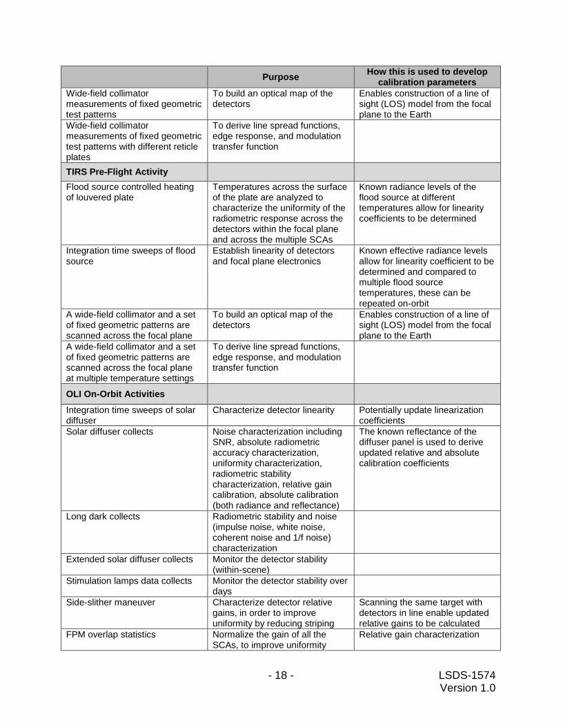
Table 3-1. Summary of Calibration Activities, Their Purpose, and How Measurements are Used in Building the Calibration Parameter Files

3.1.1 Instrument Characterization and Calibration

3.1.1.1 Description of Calibration Data Collections

A distinction is made between the calibration activities that measure, characterize, and evaluate instrument and system radiometric performance, and those which are used to derive improved radiometric processing parameters contained in the Landsat 8 Calibration Parameter File (CPF) for use by the Level 1 Product Generation System (LPGS). The measurement and evaluation activities are referred to as characterization operations, while the parameter estimation activities are referred to as calibration. Although both types of activities contribute to the “radiometric calibration” of the Landsat 8 OLI and TIRS instruments, the remainder of this document will use the term characterization to refer to radiometric assessment and evaluation operations and the term calibration to refer those associated with estimating radiometric processing parameters. Shutter Collects Shutter collects provide the individual detector dark levels or biases, which are subtracted during ground processing from each detector's response in Earth images. This removes variations in detector dark current levels reducing striping and other detector-to-detector uniformity issues in the imagery. These normal shutter collects are acquired before daylight imaging begins and after daylight imaging ends. An extended shutter collect is acquired about every three months and is about 36 minutes in duration. These longer shutter collects provide a measure of stability over typical Earth imaging intervals.

- 20 - LSDS-1574 Version 1.0

Stimulation Lamp Collects The stimulation lamps are used to monitor the detector stability over days. While incandescent lamps tend to be poor absolute calibration sources, they excel at showing changes in detector response over relatively short periods of time. There are three sets of stimulation lamps that get used at three different frequencies: daily; bi-monthly; and every six months. These different usages enable differentiation between detector changes and lamp changes. Solar Diffuser Collects The solar diffuser panels provide reflective references that were characterized prior to launch. Their regular use of the primary diffuser enables detector stability to be monitored and potential changes in calibration to be fed back into the ground processing system to maintain accuracy of the Earth imagery products. The second solar diffuser panel is used every six months as a check on stability of the primary (working) diffuser. Longer, 60 second collects of the working solar diffuser are used to monitor the within scene detector response stability. Diffuser collects are also used to characterize the system noise and SNR performance, absolute radiometric accuracy, uniformity and relative detector gains. In an additional solar diffuser data collect , the integration time sweep, a series of collects at different detector integration times is performed at a constant signal level. These collects allow an on-orbit assessment of the OLI detector electronics linearity. In an attempt to better characterize the OLI’s full detector-electronic chain linearity, two extended (60 second) diffuser collects were performed during solar eclipses (November 3, 2013 and April 29, 2014). Here, the uniform diffuser signal was obtained at a significantly lower radiance level than normal (about 40% and 10%), to allow evaluating and updating relative non-linearities between detectors. Lunar Collects Imaging the moon approximately every 28 days enables an independent measure of the OLI radiometric stability as the moon is an extremely stable source \cite{ref:moon_stability}. While the lunar surface is very stable, the viewing geometry can vary dramatically, so the lunar irradiance based model, Robotic Lunar Observatory, is used to take the viewing geometry into account. The lunar collects are also used to evaluate stray light effects and to find any other artifacts that might be visible. The moon is a good source for these artifacts since it's bright compared to the surrounding space. Side Slither Collects During a side slither data collect the spacecraft is yawed 90°, so that the normally cross track direction of the focal plane is turned along track. Here each detector in an SCA tracks over nearly identical spots on the ground. By performing these side slither maneuvers over uniform regions of the Earth, individual detector calibration coefficients can be generated to improve the pixel-to-pixel uniformity. These maneuvers are performed over desert or snow/ice regions about every three months to monitor and potentially improve the pixel-to-pixel uniformity.

- 21 - LSDS-1574 Version 1.0

Examples of characterization activities include assessments of:

the detector response to the solar diffusers, to radiometric accuracy and calibrating detector response;

the 60-second radiometric stability, to evaluate the absolute radiometric uncertainty and detect changes in detector response;

the detector response to stimulation lamp , to evaluate and detect changes in gain;

radiometric uniformity (Full field of view, banding 1, banding 2, and streaking as defined in the OLI RD) and all artifacts affecting the radiometric accuracy of the data, and SCA discontinuity differences characterized by gathering statistics information in the overlap areas between the SCAs;

deep space data and blackbody data to evaluate the absolute radiometric uncertainty of the TIRS instrument and detecting changes in gains and biases to determine radiometric stability;

dropped frames per interval, for trending the total number detected, and excluding flagged dropped frames in all characterization algorithms.

Examples of calibration activities include derivation of:

bias model parameters for each detector. The bias model for OLI is constructed using data from associated shutter images, video reference pixels, dark (masked) detectors, and associated telemetry (e.g., temperatures). The bias model for TIRS uses data from deep space images, dark (masked) detectors, and associated telemetry (e.g., temperatures). These bias model coefficients are used to derive the bias that needs to be subtracted from detector during product generation.

the relative gains for all active detectors, to correct the detector responses for "striping" artifacts;

gain determination to enable conversion from DN to radiance and determine the accuracy of the radiometric product;

the TIRS background response determination.

3.1.2 Pre-Launch

Operational Land Imager Preflight instrument performance and data characterization proceeded from subsystem level (e.g. focal plane module and electronics) to fully integrated instrument and observatory testing and analysis. Instrument testing and performance requirements verification were performed at multiple stages of development to ensure the integrity of performance at the component, subsystem, and system levels For radiometric calibration of the OLI, an integrating sphere was used as the National Institute of Standards (NIST) traceable radiance source. The OLI was connected to the integrating sphere in a configuration that enables the instrument to measure the output radiances from a prescribed set of illumination levels from xenon and halogen lamps. In

- 22 - LSDS-1574 Version 1.0

addition, integration time sweeps of full illumination at successively shorter detector exposure times were used to establish the linearity of the detectors and focal plane module electronics. Measurements of the integrating sphere at various radiance levels were also used to characterize the linearity. These and the integration time sweeps are used to determine the reciprocity between the two. Ball Aerospace and Technology Corporation (BATC), the manufacturer of the OLI, used a heliostat to facilitate the sun as a calibration source for prelaunch testing. The heliostat captured and directed sunlight from the rooftop of the BATC facility to the solar diffuser panels of the instrument placed in a thermal vacuum chamber inside the facility. The spectral reflectance and bidirectional reflectance distribution function (BRDF) of the panels were characterized at the University of Arizona. A transfer spectroradiometer was used to measure the radiances from the integrating sphere and the solar diffuser panels at the same illumination levels as measured by the OLI to ensure traceability of the measurements compared to those made from the solar diffuser panels. On orbit, any changes to the spectral response of the instrument are determined by inflight measurements of the solar diffuser panels, and coefficients used to scale the digital numbers of the instrument response to calibrated radiances can be adjusted. The signal-to-noise ratio (SNR) for each of the OLI spectral bands is characterized at a prescribed radiance level, referred to as Ltypical. The SNR is defined as the mean of the measured radiances divided by their standard deviation. A curve is fit to the SNR at the measured radiance levels and is evaluated at the prescribed Ltypical. The SNR is measured at multiple stages of the instrument build, culminating the testing of the fully integrated instrument. The high SNR combined with the 12-bit quantization of the OLI radiometric response provides data that enhance our ability to measure and monitor subtle changes in the state and condition of the Earth’s surface. The pre-launch verification of instrument and spacecraft radiometric performance specifications was carried out as part of the instrument and spacecraft manufacturers’ development, integration, and test programs. The radiometric characteristics of the OLI instrument were measured during instrument fabrication and testing at Ball Aerospace and Technologies Corporation (BATC) facility. Since the TIRS instrument is a NASA in-house development, pre-launch characterization and testing was carried out at the NASA Goddard Space Flight Center. Additional measurements and tests are being performed at Orbital Sciences Corporation (OSC) as the Landsat 8 spacecraft was being fabricated and integrated with the OLI and TIRS payloads. A Horizontal Collimator Assembly (HCA) and a set of fixed geometric patterns are scanned across the focal plane to build an optical map of the detectors which enables construction of a line of sight (LOS) model from the focal plane to the Earth. A similar process is used with a different reticle plate to derive line spread functions. These measurements assist with characterizing the alignment of detectors within a given sensor chip assembly (SCA) as well as with aligning adjacent SCAs. These are

- 23 - LSDS-1574 Version 1.0

fundamental parameters required for constructing the geometric models to achieve many of the geometric requirements. Thermal Infrared Sensor A louvered plate with stringently controlled heating wss used as a flood source and placed within the TIRS field of view so that temperatures across the surface of the plate could be analyzed to characterize the uniformity of the radiometric response across the detectors within the focal plane and across the multiple SCAs. The flood source was measured at multiple temperature levels and at multiple integration time sweeps, in order to characterize the linearity of the detector responses. A blackbody of known temperature was used as a calibration source to provide radiance to the detectors from which output voltages were converted to DNs. TIRS also measured a space-view port with a cold plate set at 170 K mounted on it, and the DNs output from the instrument were converted to radiance. The blackbody radiances were scaled by a “view factor” that was determined by viewing through the Earth-view (nadir) port. Earth view measurements were made at several temperature settings in order to establish a relationship between the temperature, DN levels, and radiance. These measurements were then combined with the blackbody and space-view measurements to derive a final set of coefficients for scaling DNs to radiances. Detector linearization is performed prior to the bias removal for TIRS because temperature contributions from instrument components are also being captured. Similar to the approach taken with OLI, a wide-field collimator and a set of fixed geometric patterns are scanned across the focal plane to build an optical map of the detectors which enables construction of a line of sight (LOS) model from the focal plane to the Earth. Instead of these targets being viewed under fixed illumination settings, these targets are presented and contrasted by controlled temperature settings. These measurements assist with characterizing the alignment of detectors within a given sensor chip assembly (SCA) as well as with aligning adjacent SCAs. These are fundamental parameters required for constructing the geometric models to achieve many of the geometric requirements.

3.1.3 Post-Launch

Radiometric characterization and calibration will be performed over the life of the mission using the software tools developed as part of the Landsat 8 Image Assessment System (IAS) and the Calibration Validation Toolkit (CVTK). The IAS provides the capability to routinely perform radiometric characterization, to verify and monitor system radiometric performance and to estimate improved values for key radiometric calibration coefficients. On-orbit activities include those that occur during the On-Orbit Initialization and Verification (OIV) period characterization and calibration and post-OIV nominal operations. Characterization activities include:

- 24 - LSDS-1574 Version 1.0

Noise – characterizing the OLI response to shutter, lamp, diffuser and lunar acquisitions, and the TIRS response to deep space views, On-Board Calibrator (OBC) collects and lunar acquisitions are used to assess various detector noise characteristics including coherent, impulse, signal-to-noise ratio (SNR), and noise equivalent delta radiance (NEDL), and ghosting.

Stability - characterizing the response of OLI to the solar diffusers, stim lamps, and lunar acquisition;, and TIRS to the (OBC) for assessing the transfer-to-orbit response, the short term (within-orbit) and long-term stability, diffuser and lunar acquisition reproducibility for OLI and post-maneuver recovery reproducibility for TIRS.

Calibration activities include:

Absolute Radiometric Response – characterizing the OLI solar diffuser, lunar irradiance, Pseudo Invariant Calibration Sites (PICS), underfly acquisitions with Landsat 7, and TIRS OBC, PICS and underfly acquisitions with Landsat 7, to assess the absolute radiometric response and deriving the initial on-orbit absolute gain CPF values.

Relative Radiometric Response - characterizing the OLI diffuser, yaw, and PICS;, and TIRS OBC, yaw and PICS sites for assessing the SCA to SCA and pixel to pixel relative response/uniformity. Special OLI diffuser and TIRS OBC integration time sweep collects are characterized to assess detector linearity, and possible updates to the CPF linearity calibration coefficients.

Key radiometric CPF parameters that may need updates are: absolute gains; relative gains, bias (default values), linearity lookup tables (LUTs), diffuser radiances (OLI), lamp radiances (OLI), OBC LUTs (TIRS), diffuser non-uniformity (OLI), OBC non-uniformity (TIRS), inoperable detectors, out-of-spec detectors, and detector select mask.

3.1.4 Operational Radiometric Tasks

The goals of these tasks are:

To demonstrate that the Landsat 8 mission meets or exceeds all radiometric requirements, particularly those that were deferred for formal verification on-orbit;

To perform an initial on-orbit radiometric calibration (relative and absolute) that makes it possible to achieve the previous goal, and that prepares the mission for routine operations;

To initialize and continue the process through nominal operations of evaluating OLI Key Performance Requirements (KPRs) by establishing an initial on-orbit performance baseline;

To trend radiometric characterization parameters throughout the mission.

- 25 - LSDS-1574 Version 1.0

3.1.4.1 OLI Characterization Tasks

A number of OLI characterizations and requirements verifications relate strictly to whether the instrument performance meets specifications, and therefore are not strongly tied to the coefficients stored in the CPF that require on-orbit updates. These requirements include: stability (60-second, 16-day), noise (overall, impulse, coherent, 1/f), stray light, ghosting, bright target recovery, detector operability, and detectors out-of-specification. Three lunar calibration acquisitions were made during the commissioning period; each acquisition comprises 15 individual image scans, performed over two consecutive orbits. Each OLI and TIRS SCA is scanned across the Moon, with one scan repeated in both orbits to provide a check on continuity of the observations. Lunar acquisitions are performed when the Earth-Sun-Moon configuration provides lunar phase angles in the -9 to -5 degree or the +5 to +9 degree ranges. The Moon traverses each phase angle range once per month, with the positive and negative angle ranges occurring approximately one day apart. In routine operations, one phase angle range is selected for all lunar acquisitions but during commissioning, both cases were collected. The timing of the commissioning period leads to three pairs of nominal lunar acquisition opportunities: one in late March 2013 just before the under-fly of Landsat 7, one in late April, 2013 after achieving the operational orbit, and one in late May 2013.

3.1.4.2 OLI Calibration Tasks

The OLI instrument was radiometrically calibrated prior to launch. The OLI viewed an integrating sphere monitored by a spectrometer that had been calibrated relative to a source that is traceable to a reference in the National Institute of Standards (NIST) Facility for Spectroradiometric Calibrations (FASCAL) facility. The gains (DN/radiance) from this calibration are stored in the CPF. The OLI’s response to the diffuser panels was measured using the sun as the source through a heliostat. Using the OLI gains, the radiance of the diffuser was measured and was corrected for the heliostat and the atmospheric transmittance to obtain a “predicted” top-of-atmosphere (TOA) radiance for the diffuser. Additionally, the OLI diffuser’s directional reflectance factors for the on-orbit illumination and view geometries were measured in the laboratory, prior to launch, giving the diffuser a reflectance calibration. These data were used to derive “prelaunch” TOA radiance calibration coefficients. The first on orbit measurements of the solar diffuser panel were compared to the “predicted” and “prelaunch” values to perform the transfer to orbit analysis. A fundamental requirement of the Landsat program is to provide a record of consistently calibrated image data. Thus OLI data need to be consistent with data from the previous Landsat sensors. Although the instruments are calibrated consistently prior to launch and monitored prior to launch through on-orbit commissioning, there is still a need to check the calibration relative to previous Landsat instruments and update the calibration parameters as necessary. Procedures were developed to characterize any shift in calibration that may occur through launch and into orbit. Two methods of validating the absolute radiometric

- 26 - LSDS-1574 Version 1.0

calibration: cross calibration with Landsat-7 ETM+ via simultaneous observations and using the pseudo-invariant calibration sites (PICS). Although generating OLI images as free of striping and banding as is practicable is one of the goals of the ground system, it cannot be expected that OLI images over uniform areas will be completely free of banding or striping, especially when extreme contrast stretches are applied. There are a number of contributors to banding and striping: inadequately characterized differential non-linear responses among detectors; inadequately characterized relative gain and bias parameters; instability in gain, bias or non-linearity; and spectral differences across or between SCAs.

3.1.4.3 TIRS Characterization Tasks

A number of TIRS characterizations and requirements verifications relate strictly to whether the instrument meets performance specifications, and therefore are not strongly tied to the coefficients stored in the CPF that require on-orbit updates. These requirements include: stability (60 second, 16-day); noise (overall, impulse, coherent, 1/f); stray light; ghosting; bright target recovery; detector operability; and detectors out-of-specification. Three lunar acquisitions were performed during the commissioning period. Each acquisition comprises 15 individual image scans, performed over two consecutive orbits. Each TIRS SCA is scanned across the Moon, with one scan repeated in both orbits to provide a check on continuity of the observations. As with OLI, the TIRS lunar acquisitions are performed when the Earth-Sun-Moon configuration provides lunar phase angles in the -9 to -5 degree or the +5 to +9 degree ranges.). During the operational mission lifetime lunar acquisitions will be performed monthly as defined for the OLI.

3.1.4.4 TIRS Calibration Tasks

Thus TIRS data need to be consistent with data from the previous sensors, so by extension, Landsat 8 TIRS data needs to be cross-calibrated with Landsat-7 ETM+ data. At least two techniques will be used for this comparison and calibration i.e. simultaneous data acquisitions collected during the under-fly of Landsat 7, and non-simultaneous observation of well-characterized targets. TIRS was carefully characterized and calibrated prior to launch and procedures were developed to be able to characterize any shift in calibration that may occur during launch and insertion into orbit. TIRS Relative Response - Uniformity Evaluation As with the OLI, there are a number of factors that may contribute to banding and striping in TIRS imagery: inadequately characterized differential non-linearity among detectors; inadequately characterized relative gain and bias; instability in gain, bias or non-linearity; and spectral differences across or between SCAs.

3.2 Geometric Calibration Overview

This section describes the geometric characterization and calibration activities that are performed over the life of the Landsat 8 mission using the software tools developed as

- 27 - LSDS-1574 Version 1.0

part of the Landsat 8 Image Assessment System (IAS). The IAS provides the capability to routinely perform four types of geometric characterization to verify and monitor system geometric performance, and four types of geometric calibration to estimate improved values for key system geometric parameters. These are the parameters contained in the Calibration Parameter File (CPF) for use in the level 1 product generation. The measurement and evaluation activities are referred to as characterization operations, while the parameter estimation activities are referred to as calibration. The geometric characterizations include:

1. Assessment of the absolute and relative geodetic accuracy of Level 1G data (Geodetic Characterization);

2. Assessment of the geometric accuracy of Level 1T products (Geometric Characterization);

3. Assessment of the accuracy of multi-temporal OLI image-to-image registration (Image-to-Image Registration Characterization);

4. Assessment the accuracy of OLI and TIRS band-to-band registration (Band-to-Band Registration Characterization).

A fifth characterization algorithm will be used to evaluate OLI spatial performance on-orbit. This modulation transfer function (MTF) bridge characterization algorithm uses images of selected ground targets (e.g., the Lake Pontchartrain Causeway) to estimate the OLI sensor edge response. The characterizations performed during the commissioning period were used to establish an OLI performance baseline to serve as a basis for comparison in evaluating the OLI key performance requirements (KPRs) throughout the life of the mission. The characterizations of primary interest as KPRs are OLI band registration accuracy and spatial performance. The geometric calibrations include:

1. Determination of the alignment between the spacecraft navigation reference frame and the OLI payload line of sight (Sensor Alignment Calibration);

2. Determination of corrections to the pre-launch OLI panchromatic band lines of sight, including relative alignment of the OLI sensor chip assemblies (OLI Focal Plane Calibration);

3. Determination of the alignment between the TIRS and OLI sensors, including the relative alignment of the TIRS sensor chip assemblies (TIRS Alignment Calibration).

4. Determination of corrections to the band location field angles for both OLI and TIRS (Band Alignment Calibration).

The most critical geometric calibration activities are to measure and verify the Landsat 8 spacecraft, OLI, and TIRS system performance using the geodetic, geometric, band-to-band, image-to-image, and spatial characterization capabilities; to monitor the OLI sensor to spacecraft attitude control system alignment calibration; and to monitor the

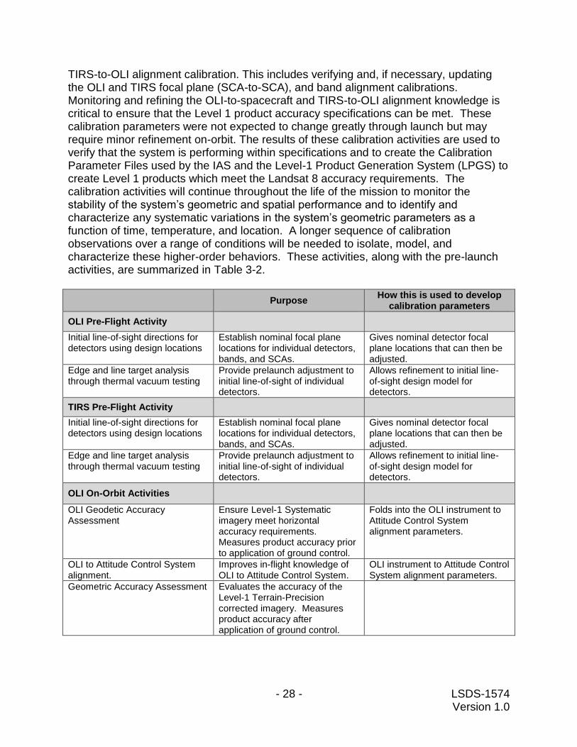
- 28 - LSDS-1574 Version 1.0

TIRS-to-OLI alignment calibration. This includes verifying and, if necessary, updating the OLI and TIRS focal plane (SCA-to-SCA), and band alignment calibrations. Monitoring and refining the OLI-to-spacecraft and TIRS-to-OLI alignment knowledge is critical to ensure that the Level 1 product accuracy specifications can be met. These calibration parameters were not expected to change greatly through launch but may require minor refinement on-orbit. The results of these calibration activities are used to verify that the system is performing within specifications and to create the Calibration Parameter Files used by the IAS and the Level-1 Product Generation System (LPGS) to create Level 1 products which meet the Landsat 8 accuracy requirements. The calibration activities will continue throughout the life of the mission to monitor the stability of the system’s geometric and spatial performance and to identify and characterize any systematic variations in the system’s geometric parameters as a function of time, temperature, and location. A longer sequence of calibration observations over a range of conditions will be needed to isolate, model, and characterize these higher-order behaviors. These activities, along with the pre-launch activities, are summarized in Table 3-2.



OLI Pre-Flight Activity

Initial line-of-sight directions for detectors using design locations

Establish nominal focal plane locations for individual detectors, bands, and SCAs.

Gives nominal detector focal plane locations that can then be adjusted.

Edge and line target analysis through thermal vacuum testing

Provide prelaunch adjustment to initial line-of-sight of individual detectors.

Allows refinement to initial line-of-sight design model for detectors.

TIRS Pre-Flight Activity

Initial line-of-sight directions for detectors using design locations

Establish nominal focal plane locations for individual detectors, bands, and SCAs.

Gives nominal detector focal plane locations that can then be adjusted.

Edge and line target analysis through thermal vacuum testing

Provide prelaunch adjustment to initial line-of-sight of individual detectors.

Allows refinement to initial line-of-sight design model for detectors.

OLI On-Orbit Activities

OLI Geodetic Accuracy Assessment

Ensure Level-1 Systematic imagery meet horizontal accuracy requirements. Measures product accuracy prior to application of ground control.

Folds into the OLI instrument to Attitude Control System alignment parameters.

OLI to Attitude Control System alignment.

Improves in-flight knowledge of OLI to Attitude Control System.

OLI instrument to Attitude Control System alignment parameters.

Geometric Accuracy Assessment Evaluates the accuracy of the Level-1 Terrain-Precision corrected imagery. Measures product accuracy after application of ground control.

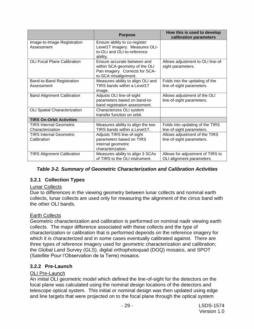
- 29 - LSDS-1574 Version 1.0



Image-to-Image Registration Assessment

Ensure ability to co-register Level1T imagery. Measures OLI-to-OLI and OLI-to-reference ability.

OLI Focal Plane Calibration Ensure accurate between and within SCA geometry of the OLI Pan imagery. Corrects for SCA-to-SCA misalignment.

Allows adjustment to OLI line-of-sight parameters.

Band-to-Band Registration Assessment

Measures ability to align OLI and TIRS bands within a Level1T image.

Folds into the updating of the line-of-sight parameters.

Band Alignment Calibration Adjusts OLI line-of-sight parameters based on band-to-band registration assessment.

Allows adjustment of the OLI line-of-sight parameters.

OLI Spatial Characterization Characterizes OLI system transfer function on orbit.

TIRS On-Orbit Activities

TIRS Internal Geometric Characterization

Measures ability to align the two TIRS bands within a Level1T.

Folds into updating of the TIRS line-of-sight parameters.

TIRS Internal Geometric Calibration

Adjusts TIRS line-of-sight parameters based on TIRS internal geometric characterization.

Allows adjustment of the TIRS line-of-sight parameters.

TIRS Alignment Calibration Measures ability to align 3 SCAs of TIRS to the OLI instrument.

Allows for adjustment of TIRS to OLI alignment parameters.

Table 3-2. Summary of Geometric Characterization and Calibration Activities

3.2.1 Collection Types

Lunar Collects Due to differences in the viewing geometry between lunar collects and nominal earth collects, lunar collects are used only for measuring the alignment of the cirrus band with the other OLI bands. Earth Collects Geometric characterization and calibration is performed on nominal nadir viewing earth collects. The major difference associated with these collects and the type of characterization or calibration that is performed depends on the reference imagery for which it is characterized and in some cases eventually calibrated against. There are three types of reference imagery used for geometric characterization and calibration; the Global Land Survey (GLS), digital orthophotoquad (DOQ) mosaics, and SPOT (Satellite Pour l’Observation de la Terre) mosaics.

3.2.2 Pre-Launch

OLI Pre-Launch An initial OLI geometric model which defined the line-of-sight for the detectors on the focal plane was calculated using the nominal design locations of the detectors and telescope optical system. This initial or nominal design was then updated using edge and line targets that were projected on to the focal plane through the optical system

- 30 - LSDS-1574 Version 1.0

during prelaunch thermal vacuum testing. This model was then considered an as-built prelaunch set of line of sights for each detector for which each band for each SCA could be adjusted post launch using the IAS geometric characterization and calibration processes. TIRS Pre-Launch An initial TIRS geometric model, consisting of detector and sensor chip assembly within the focal plane along with the optics of the telescope, was determined based upon its’ assembly through instrument and component design and final integration to the spacecraft. This included the focal plane and detector placement, the telescope and optical components, and the TIRS-to-spacecraft alignment measurements. These components were then updated during prelaunch using measurements taking during thermal vacuum testing. Targets were projected into the TIRS field of view at operator selectable locations allowing for careful identification of both the target within the focal plane and the origination of the target itself. This model was then considered an as-built prelaunch set of line of sights for each detector for which each band for each SCA could be adjusted post launch using the IAS geometric characterization and calibration processes.

3.2.3 OLI Geodetic Accuracy Assessment

The purpose of the geodetic accuracy assessment is to ensure that the Landsat 8 Level 0R data can be successfully processed into Level 1 systematic products that meet the system requirement of 65 meters at a circular error with 90% confidence (CE90) horizontal accuracy. Pre-defined ground control points (consisting of image chips with known geodetic positions are automatically correlated with data from the OLI SWIR1 (for Global Land Survey 2000-based (GLS2000) control) or panchromatic bands (for digital orhtophotoquad (DOQ) control) to measure the discrepancy between the known ground location and the position predicted by the OLI geometric model. The results of the control point mensuration are used for analysis by the IAS geodetic characterization software. The precision correction software also combines the estimated attitude error from the precision solution with the current best estimate of OLI-to-spacecraft alignment from the CPF, to compute the adjusted alignment that would make the resulting attitude error zero. This apparent alignment is stored in the geometric trending database for subsequent use by the sensor alignment calibration procedures. The geodetic accuracy characterization software processes the control point residuals (deleting those identified as outliers) to generate summary statistics and a geodetic accuracy analysis report each time the precision correction solution process is successfully completed. The geodetic accuracy results are stored in the geometric characterization trending database with a flag to indicate the control type used (GLS or DOQ).

- 31 - LSDS-1574 Version 1.0

3.2.4 Sensor Alignment Calibration

The goal of the sensor alignment calibration is to improve the in-flight knowledge of the relationship between the OLI instrument and the spacecraft attitude control system reference frame. Sensor alignment calibration uses the results of the ground control point processing conducted both as part of routine L1T product generation (using GLS2000 control) and as part of calibration/validation analysis activities over geometric calibration sites (using DOQ control). The end-to-end OLI geolocation accuracy error budget assumes that the IAS is able to estimate this alignment to an accuracy of 33 microradians (3-sigma) over periods as short as one 16-day WRS-2 cycle. The potential need for a sensor alignment calibration updates will be identified by monitoring the geodetic accuracy characterization results. If persistent geolocation accuracy biases are observed, then that would suggest the need for generating an updated sensor alignment matrix for inclusion in the Calibration Parameter File. Automated software tools are used to detect the existence of a new alignment calibration solution and to perform automated testing of the new and old calibration solutions against a set of test scenes extracted from the list of retrieved alignment calibration scenes. A new alignment matrix will be generated whenever a new version of the CPF is scheduled for release, nominally on a quarterly basis, therefore any slowly varying seasonal alignment variations will be accounted for.

3.2.5 Geometric Accuracy Assessment

The purpose of the geometric accuracy assessment is to evaluate the accuracy of Level 1T image products using an independent set of ground control points. Although the geodetic accuracy characterization results report both the pre- and post-GCP correction scene accuracy statistics, the post-fit statistics are not an unbiased estimate of the actual accuracy of the corrected scene. An independent geometric accuracy assessment is performed by correlating the final L1T product with a separate set of GCPs that were withheld from the original precision correction solution. Scenes for which the number of available GCPs was too small to permit withholding some from the precision correction process do not have validation points. The geometric accuracy assessment procedure is run as a part of the standard L1T product generation flow.

3.2.6 OLI Internal Geometric Characterization and Calibration

OLI internal geometric accuracy refers to internal geometric distortions within the OLI images due to errors in the relative alignment of the 14 sensor chip assemblies (SCAs), also known as focal plane modules (FPMs), on the OLI focal plane. If the OLI line-of-sight model knowledge of the pointing for each SCA is slightly inaccurate, this will result in internal geometric distortions in the L1T products and, potentially, visible image discontinuities at SCA boundaries. Although the OLI LOS model is carefully characterized pre-launch, tools are available to detect and, if necessary, correct any SCA-to-SCA misalignment that may be observed by updating the OLI LOS model calibration. These tools are implemented in the IAS as the image-to-image registration accuracy characterization and the OLI focal plane calibration algorithms.

- 32 - LSDS-1574 Version 1.0

The OLI panchromatic band is used as the geometric reference for the entire instrument. The image-to-image registration accuracy and the pattern of registration errors may indicate the presence of unwanted internal distortions in the OLI image that could be addressed by refining the OLI focal plane calibration. The following subsections describe the details of the image-to-image registration assessment and OLI focal plane calibration procedures individually.

3.2.6.1 Image-to-Image Registration Assessment

The goal of the image-to-image registration assessment is to verify the Landsat 8 requirement that multi-temporal images of the same WRS scene can be successfully co-registered to an accuracy of 0.4 (LE90) multispectral pixels (i.e., 12 meters). The image-to-image assessment procedure uses ground control points that have either been extracted from a previously generated L1T image, or that match the points used to correct the pre-existing L1T product, to perform precision and terrain correction of a new acquisition to Level 1T. It then performs a point-by-point comparison of the two images using automated image correlation. Image-to-image registration assessment using the panchromatic band demonstrates the accuracy of the overall precision correction solution as well as the internal geometric fidelity of the images.

3.2.6.2 OLI Focal Plane Calibration

The OLI focal plane calibration is intended to detect and measure systematic deviations of the OLI lines-of-sight for each SCA from the model measured during pre-launch characterization. Any significant deviations detected will be folded back into the Calibration Parameter file as updates to the LOS model Legendre polynomial coefficients.

3.2.6.3 Band-to-Band Registration Assessment

The band-to-band registration assessment measures the relative alignment of the nine OLI and two TIRS spectral bands after processing to L1T to verify that the 4.5 meter (LE90) OLI, 18 meter (LE90) TIRS, and 30 meter (LE90) OLI-to-TIRS band-to-band registration requirements are met.

3.2.6.4 Band Alignment Calibration

The purpose of band placement calibration is to estimate improved values for the locations of the spectral bands on the OLI and TIRS focal planes for inclusion in the Calibration Parameter File. The band locations are embodied in the LOS model Legendre coefficients for each OLI and TIRS band/SCA. OLI and TIRS band alignment use essentially the same algorithm but would be processed separately. The panchromatic band is used as the reference for the OLI solution since it is the band used to perform the (sensor alignment and focal plane calibrations. TIRS band 10 is

- 33 - LSDS-1574 Version 1.0

used as the reference for TIRS band alignment since it is also used in TIRS alignment calibration The OLI cirrus band is only used for lunar and high altitude terrestrial targets.

3.2.7 TIRS Internal Geometric Characterization and Calibration

The TIRS geometric alignment calibration procedure accomplishes both internal and external geometric alignment calibration for the TIRS instrument. TIRS internal geometric accuracy can be degraded by internal geometric distortions within the TIRS images due to errors in the relative alignment of the 3 sensor chip assemblies (SCAs) on the TIRS focal plane. If the TIRS line-of-sight model knowledge of the pointing for each SCA is slightly inaccurate, this will result in internal geometric distortions in the L1T product images and, potentially, visible image discontinuities at SCA boundaries. TIRS external geometric accuracy refers to the accuracy with which TIRS data can be registered to corresponding OLI data and to an absolute ground coordinate system. This accuracy is primarily dependent on accurate knowledge of the alignment between the OLI and TIRS instruments. The alignments of both the OLI and TIRS instruments relative to the spacecraft ACS frame were measured during observatory integration, but due to the accuracy limitations of these measurements and the likelihood of launch shift and zero-G release altering these alignments, on-orbit TIRS alignment estimation was updated to achieve the TIRS geometric accuracy requirements. Although the TIRS LOS model was also carefully characterized pre-launch, TIRS alignment calibration provides the tools needed to detect and, if necessary, correct any SCA-to-SCA misalignment that may be observed while updating the TIRS LOS model calibration. The TIRS 10.8 micron band (band 10) is used as the geometric reference for aligning the TIRS instrument to the OLI. Band 10 is also used as the reference band in TIRS band alignment calibration, as noted above. As the TIRS geometric reference, internal SCA-to-SCA focal plane alignment is also performed using band 10. The following subsection describes the details of the TIRS alignment calibration procedure.

3.2.7.1 TIRS Alignment Calibration

The TIRS alignment calibration measures systematic deviations of the TIRS lines-of-sight for each SCA from the model measured during pre-launch characterization while simultaneously measuring the global misalignment of all three TIRS SCAs relative to the OLI. These measurements are used to compute updates to the TIRS-to-OLI and, indirectly, TIRS-to-ACS alignment matrices as well as updates to the TIRS LOS model Legendre polynomial coefficients, with the results being folded back into the Calibration Parameter file. A control reference image of coincident OLI SWIR bands with good emissive-to-reflective band correlation is used for calibration. The TIRS alignment calibration procedure compares a precision and terrain corrected TIRS band 10 SCA-separated

- 34 - LSDS-1574 Version 1.0

image with a coincident OLI SWIR1 band SCA-combined reference image processed with the same spacecraft geometric model and scene framing parameters. This enables measurement of the overall TIRS-to-OLI alignment, as well as the relative alignment of the individual TIRS SCAs.

3.2.8 OLI Spatial Performance Characterization

OLI spatial performance, expressed as the slope and width of the instrument’s response to a unit edge/step function, was carefully characterized during pre-launch testing. The experience of the Landsat 7 ETM+, which suffered from gradually degrading spatial fidelity over the first several years of on-orbit operations, led to the development of an algorithm to measure and track on-orbit spatial performance. This was done by using long bridge targets to characterize the ETM+ modulation transfer function (MTF), which is the frequency domain representation of the instrument’s spatial response. This algorithm was subsequently adapted for use with push-broom sensors using Advanced Land Imager (ALI) data and it is a variant of this adapted algorithm that will be used for OLI spatial characterization. A method for using lunar scans to characterize ALI spatial performance was also developed but the results were not sufficiently reliable for use in operational performance characterization There are no calibration activities associated with spatial performance, although the OLI does have ground-commandable focus mechanisms and TIRS focus can be adjusted by changing telescope temperatures. To support on-orbit focus verification, additional focus test sites have been identified to provide qualitative information about the state of OLI and TIRS focus during the commissioning period. These sites are listed in Appendix A and were selected to contain distinct targets that could be used for visual assessment as well as additional sites for quantitative analysis using the enhanced version of the spatial performance characterization algorithm. Combined with the quantitative results of the spatial performance characterization algorithm, visual inspection of the focus sites adds confidence that the OLI and TIRS are in proper focus. The derivation of any adjustments to the focus mechanism positions or TIRS telescope temperatures that may be required to improve on-orbit spatial performance would require additional analysis that is beyond the scope of this algorithm. Spatial edge slope performance in all OLI bands (other than the cirrus band) is a Key Performance Requirement (KPR) for OLI on-orbit performance. The derived spatial performance parameters can then be compared to the thresholds specified in the corresponding KPR to evaluate on-orbit performance. The precision of the on-orbit spatial performance estimates is such that repeated measurements are required to establish the validity that the standard performance level of any requirement is not met.

3.2.9 OLI Bridge Target MTF Estimation

The purpose of the OLI bridge target MTF estimation procedure is to use OLI acquisitions of prescribed bridge targets to derive on-orbit estimates of the OLI system transfer function for each OLI spectral band other than the cirrus band. The system transfer function (STF) estimates are then used to compute the corresponding point spread function and edge response slope performance for each spectral band. The OLI

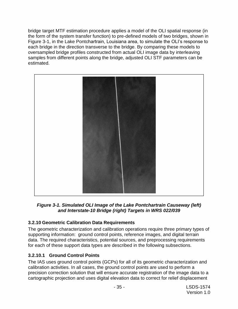
- 35 - LSDS-1574 Version 1.0

bridge target MTF estimation procedure applies a model of the OLI spatial response (in the form of the system transfer function) to pre-defined models of two bridges, shown in Figure 3-1, in the Lake Pontchartrain, Louisiana area, to simulate the OLI’s response to each bridge in the direction transverse to the bridge. By comparing these models to oversampled bridge profiles constructed from actual OLI image data by interleaving samples from different points along the bridge, adjusted OLI STF parameters can be estimated.

3.2.10 Geometric Calibration Data Requirements

The geometric characterization and calibration operations require three primary types of supporting information: ground control points, reference images, and digital terrain data. The required characteristics, potential sources, and preprocessing requirements for each of these support data types are described in the following subsections.

3.2.10.1 Ground Control Points

The IAS uses ground control points (GCPs) for all of its geometric characterization and calibration activities. In all cases, the ground control points are used to perform a precision correction solution that will ensure accurate registration of the image data to a cartographic projection and uses digital elevation data to correct for relief displacement

Figure 3-1. Simulated OLI Image of the Lake Pontchartrain Causeway (left) and Interstate-10 Bridge (right) Targets in WRS 022/039

- 36 - LSDS-1574 Version 1.0

in the process. The IAS and LPGS both access a database of GCPs. These points were adopted from the Landsat 7 mission and include both the global GCP set extracted from the Global Land Survey (GLS) data and the higher precision control points extracted from geometric calibration reference data (e.g., digital orthophotoquad (DOQ) mosaics, SPOT data). GCPs from either or both control sets can be extracted by control type: GLS or DOQ (DOQ is used as a generic type indicator for all GCPs extracted from geometric calibration sources). The GLS control database covers essentially every land scene observed from the WRS-2 orbit. The control derived from the GLS is accurate to approximately 20 meters root mean square error (RMSEr) absolute, but since the goal is to make Landsat 8 products that are consistent with the other products generated from the archive of historical data. GLS GCPs include image chips extracted from the ETM+ band 5 at 30 meter GSD and have also been automatically subdivided into separate CONTROL and VALIDATION subsets in scenes where a sufficient number of points were available. The DOQ control database only covers scenes designated as geometric calibration sites. There are two main clusters of these sites. The first set is in the United States, and was selected to provide at least one acquisition opportunity on every WRS-2 cycle day, including a group in the south-western U.S. that are at approximately the same latitude to provide consistent acquisition conditions (position in orbit, ETM+ time-on). These contain control extracted from reduced resolution DOQ data (panchromatic, 15 meter GSD). A second group of control scenes are in the eastern half of Australia. This control set is based upon mosaics of SPOT panchromatic data provided by GeoScience Australia’s National Earth Observation Group (NEOG). Being in the southern hemisphere, this set provides somewhat different orbital geometry and thermal conditions than the U.S. set. One of the primary purposes of the DOQ control set is to ensure accurate registration between Landsat 8 L1T products and the DOQ- and SPOT-derived reference imagery (discussed below) used for focal plane calibration. The GLS control points were extracted from the GLS 2000 ETM+ images using an automated interest operator technique that selected points based on a local spatial operator that identified “interesting” points, and a spatial distribution test that decided which points provided the best distribution of control across the scene. A subsequent test was added to weed out points that contained only water. The GLS control has been in routine operational use for generating Landsat 5 and Landsat 7 standard L1T data products. An important note is that the GLS images themselves were generated based upon a global block triangulation of Landsat 7 scenes with a sparse set of ground control provide by the National Geospatial-Intelligence Agency (NGA). The scenes that contained NGA control are more accurate than those that were positioned solely through triangulation. The NGA-controlled scene subset will therefore be given special attention when mining the geodetic accuracy and sensor alignment data for systematic within-orbit effects. The DOQ control points were extracted from the DOQ mosaic reference images (U.S. set) and the SPOT mosaic reference image (Australia) and therefore inherit the

- 37 - LSDS-1574 Version 1.0

accuracy of those products. Since the primary purpose of these points is to ensure good OLI to reference image registration, the absolute accuracy of these points, though believed to be better than the GLS control, is of less interest. The list of geodetic characterization sites where DOQ control points are available is included in Appendix A.

3.2.10.2 Reference Images

Two types of reference images are used by the geometric super-site calibration operations described above. The first type are previously generated Landsat 8 L1T products used in the image-to-image registration assessment process. These reference images were generated by processing L0R data through the IAS Level 1 processing software after launch, and are not discussed further here. The second type of reference images were constructed pre-launch using a high resolution image source. These images are used to provide the reference for OLI focal plane calibration as described above. These reference images are the subject of the remainder of this section. The key characteristics of the focal plane calibration reference images are: 1) high absolute geodetic accuracy (including removal of any terrain displacement effects); 2) internal geometric integrity (no systematic internal distortions which could be confounded with OLI focal plane alignment effects); 3) spectral similarity to the OLI panchromatic band; 4) resolution as good or better than the OLI panchromatic band; and 5) availability in areas of minimal seasonal change and low average cloud cover. Geodetic accuracy of one-half of a panchromatic pixel (7.5 meters) should be sufficient although higher accuracy is desirable. The internal geometric accuracy requirement disqualifies ETM+ data as a source of reference imagery, though in an emergency ETM+ reference data (e.g., GLS) would be better than nothing. High resolution panchromatic imagery from aerial photographs which meet the geodetic accuracy requirement have been available for years. Panchromatic satellite imagery is available from SPOT and a number of high resolution commercial missions, but the cost associated with acquiring the volume of data required to cover a Landsat scene has limited the application of these sources to a set of sites in Australia where GeoScience Australia’s National Earth Observation Group (NEOG) have provided full WRS-2 scene SPOT data coverage. The preferred source of high resolution reference imagery based upon availability and cost are the Digital Orthophoto Quadrangles (DOQ) produced under contract to the USGS. The DOQs are created by digitizing and orthorectifying panchromatic aerial photography. The DOQ products are distributed as 3.75 arc-minute quarter quads at 1-meter resolution. The DOQ geodetic accuracy is specified to meet National Map Accuracy Standards (NMAS) for 1:24,000-scale maps. This standard calls for a circular error (CE) of 40 feet at the 90% confidence level, which converts to approximately 6 meters CE one sigma, and meets the one-half OLI pixel requirement. DOQ data coverage has improved since the launch of Landsat 7, to the point where it is now possible to generate a DOQ reference image nearly everywhere in the conterminous U.S. Though still time consuming to construct, this has made it possible to assemble

- 38 - LSDS-1574 Version 1.0

sufficient DOQ reference sites to provide at least one acquisition opportunity on every WRS-2 cycle day. SPOT data, though not quite as accurate as the DOQ data, are available globally. The primary drawback of using SPOT data is the cost. Fortunately, our colleagues at GeoScience Austratlia were good enough to provide several Landsat scene-sized mosaics of SPOT data in Australia for use in Landsat 5 and 7 bumper-mode calibration. These reference images will continue to be used for OLI focal plane calibration, though they can be expected to become less useful over time as the imagery become outdated.

3.2.10.3 Terrain Data

Digital terrain data are needed to provide the elevation information used by the IAS (and LPGS) Level 1 terrain correction process. Terrain corrected images are used in all of the geometric calibration operations described above. The elevation information must completely cover the geometric calibration sites to support the terrain correction process. The height values must be referenced to the WGS84 ellipsoid rather than mean sea level to be consistent with the ground control height values. Vertical accuracy better than 15 meters (one sigma) is desirable. This keeps terrain-induced errors below 0.1 panchromatic pixels at the edges of the OLI field of view. An accuracy of 30 meters (one sigma) is acceptable. For product generation purposes it is also desirable that the elevation data used be consistent with the GLS 2000 reference data set. The digital elevation model (DEM) data used to generate the GLS datasets meets these requirements. Assembling a global elevation data set suitable for generating a global Landsat image base was a primary objective of the GeoCover (which evolved into the Global Land Survey) project . This resulted in a global DEM constructed from the best available source data, including the USGS National Elevation Dataset (NED) DEM data, the Canadian Digital Elevation Dataset (CDED), the NASA/NGA Shuttle Radar Topography Mission (SRTM) data, and NGA Digital Terrain Elevation Data (DTED) products. The GLS DEM provides a globally (mostly) consistent elevation dataset that corresponds to the GLS imagery that defines the Landsat 8 geometric reference. Tools were developed to retrieve any specified land area from the global DEM, so the elevation data sets required to process any given scene (nadir-viewing or off-nadir) are extracted and assembled on demand from the GLS archive. The digital terrain data for the desired output product area are extracted from the GLS DEM archive, as noted above, and then be preprocessed into the output space used for the calibration test scene. This DEM resampling step is part of the normal Level 1 processing sequence.

3.3 Calibration Parameters

The Calibration and Validation Team (CVT) is responsible for the sustained radiometric and geometric calibration of the Landsat 8 satellite and the TIRS and OLI sensors. This is achieved by assessing new imagery on a daily basis, performing both radiometric and geometric calibration when needed, and developing new processing parameters for creating Level 1 (L1) products. Processing parameters are stored in the Calibration Parameter File (CPF), the Response Linearity Look-Up Table (RLUT) and the Bias

- 39 - LSDS-1574 Version 1.0

Parameter File (BPF), which are stamped with effectivity dates and bundled with Level 0R (L0R) products.

3.3.1 Calibration Parameter File

The CVT updates the CPF at least every three months. Updates will likely be more frequent during early orbit checkout and will also occur between the regular three month cycles whenever necessary. Irregular updates will not affect the regular schedule. The timed release of a new CPF must be maintained because of the UT1 time corrections and pole wander predictions included in the file. These parameters span a 180 days and includes approximately 45 days before and 45 days after the effective start date of each CPF. The IAS maintains an archive of CPFs, which can be accessed at: http://landsat.usgs.gov/calibration_notices.php. The CPF is time-stamped with an effective date range. The parameters in the file—Effective_Date_Begin and Effective_Date_End—designate the range of valid acquisition dates and are in YYYY-MM-DDThh:mm:ss format (ISO 8601). The parameter file used in processing an image requires an effective date range that includes the acquisition date of the ordered image. Through the course of the mission, a serial collection of CPFs is generated and made available for download. Calibration Parameter Files are replaced when improved calibration parameters for a given period are developed. The need for unique file sequence numbers becomes necessary as file contents change. Version numbers for all effective date ranges after the launch begin with 01. The following is an example of the file naming procedure:

L8CPFyyyy1mm

1dd

1_yyyy

2mm

2 dd

2.nn

L Constant for Landsat

8 Satellite numerical representation

CPF Three-letter CPF designator

yyyy1 Four-digit effective starting year

mm1 Two-digit effective starting month

dd1 Two-digit effective starting day

_ Effective starting/ending date separator

yyyy2 Four-digit effective ending year

mm2 Two-digit effective ending month

dd2 Two-digit effective ending day

. Ending day/version number separator

nn Version number for this file

As an example, suppose four calibration files were created on 90-day intervals, the first file updated twice, and the second and third files updated once since 2012; the assigned file names would be as follows: File 1 L8CPF20120101_20120331.01 L8CPF20120101_20120331.02 L8CPF20120101_20120331.03

http://landsat.usgs.gov/calibration_notices.php

- 40 - LSDS-1574 Version 1.0

File 2 L8CPF20120401_20120630.01 L8CPF20120401_20120630.02 File 3 L8CPF20120701_20120930.01 L8CPF20120701_20120930.02 File 4 L8CPF20121001_20121231.01 The reserved sequence number 00 uniquely identifies the pre-launch CPF. Sequence numbers for subsequent time periods all begin with 01. New versions or updates are incremented by one. This example assumes the effectivity dates do not change. The effectivity date range for a file can change if an instrument change event is discovered within the nominal three month effectivity range. Assuming this scenario, two CPFs with new names and effective dates are spawned for the time period under consideration. The effective_date_end for a new pre-event CPF would change to the day before the problem occurred. The effective_date_begin remains unchanged. A post-event CPF with a new file name would be created with an effective_date_begin corresponding to the imaging date the problem occurred. The effective_date_end would be set to the original effective_date_end for the time period under consideration. New versions of all other CPFs affected by the parameter change also would be created. The version numbers continue to increment from the original unsplit CPF. Using this example, suppose a dead detector is discovered to have occurred on July 25, 2012. Two new CPFs are created that supersede the time period represented by file number three, version 2, and a new version of file number four is created. The new file names and sequence numbers become: File 3 L8CPF20120701_20120930.01 L8CPF20120701_20120930.02 L8CPF20120701_20120724.03 L8CPF20120725_20120930.03 File 4 L8CPF20121001_20121231.01 L8CPF20121001_20121231.02

3.3.1.1 File Structure

All calibration parameters are stored as American Standard Code for Information Interchange (ASCII) text using the Object Definition Language (ODL) syntax developed by the NASA JPL. ODL is a tagged keyword language developed to provide a human-readable data structure to encode data for simplified interchange. The body of the file is composed of two statement types:

1. Attribute assignment statement used to assign values to parameters. 2. Group statements used to aid in file organization and enhance parsing

granularity of parameter sets. To illustrate consider the first nine parameters in the file, these nine parameters form their own group, which is called FILE_ATTRIBUTES. The syntax employed for this collection of parameters in the CPF appears as:

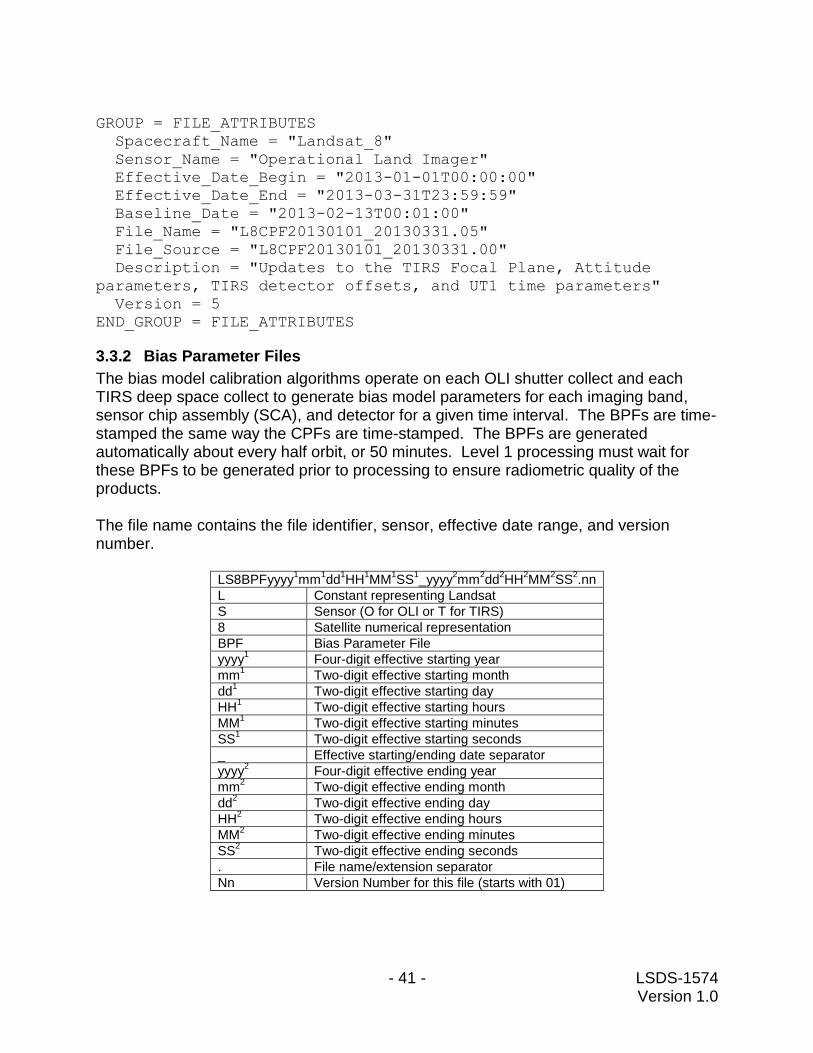
- 41 - LSDS-1574 Version 1.0

GROUP = FILE_ATTRIBUTES

Spacecraft_Name = "Landsat_8"

Sensor_Name = "Operational Land Imager"

Effective_Date_Begin = "2013-01-01T00:00:00"

Effective_Date_End = "2013-03-31T23:59:59"

Baseline_Date = "2013-02-13T00:01:00"

File_Name = "L8CPF20130101_20130331.05"

File_Source = "L8CPF20130101_20130331.00"

Description = "Updates to the TIRS Focal Plane, Attitude

parameters, TIRS detector offsets, and UT1 time parameters"

Version = 5

END_GROUP = FILE_ATTRIBUTES

3.3.2 Bias Parameter Files

The bias model calibration algorithms operate on each OLI shutter collect and each TIRS deep space collect to generate bias model parameters for each imaging band, sensor chip assembly (SCA), and detector for a given time interval. The BPFs are time-stamped the same way the CPFs are time-stamped. The BPFs are generated automatically about every half orbit, or 50 minutes. Level 1 processing must wait for these BPFs to be generated prior to processing to ensure radiometric quality of the products. The file name contains the file identifier, sensor, effective date range, and version number.

LS8BPFyyyy1mm

1dd

1HH

1MM

1SS

1_yyyy

2mm

2dd

2HH

2MM

2SS

2.nn

L Constant representing Landsat

S Sensor (O for OLI or T for TIRS)


BPF Bias Parameter File




HH1 Two-digit effective starting hours

MM1 Two-digit effective starting minutes

SS1 Two-digit effective starting seconds





HH2 Two-digit effective ending hours

MM2 Two-digit effective ending minutes

SS2 Two-digit effective ending seconds

. File name/extension separator

Nn Version Number for this file (starts with 01)

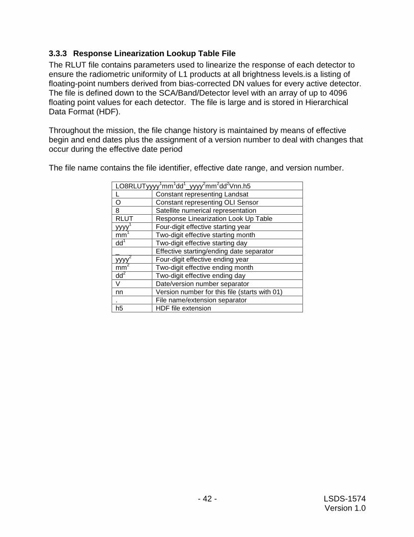
- 42 - LSDS-1574 Version 1.0

3.3.3 Response Linearization Lookup Table File

The RLUT file contains parameters used to linearize the response of each detector to ensure the radiometric uniformity of L1 products at all brightness levels.is a listing of floating-point numbers derived from bias-corrected DN values for every active detector. The file is defined down to the SCA/Band/Detector level with an array of up to 4096 floating point values for each detector. The file is large and is stored in Hierarchical Data Format (HDF). Throughout the mission, the file change history is maintained by means of effective begin and end dates plus the assignment of a version number to deal with changes that occur during the effective date period The file name contains the file identifier, effective date range, and version number.

LO8RLUTyyyy1mm

1dd

1_yyyy

2mm

2dd

2Vnn.h5

L Constant representing Landsat

O Constant representing OLI Sensor


RLUT Response Linearization Look Up Table








V Date/version number separator

nn Version number for this file (starts with 01)

. File name/extension separator

h5 HDF file extension

- 43 - LSDS-1574 Version 1.0

Section 4 Level 1 Products

4.1 Level 1 Product Generation

4.1.1 Overview

The geometric algorithms used by Level-1 Product Generation System (LPGS) at EROS were originally developed for the Landsat 8 Image Assessment System (IAS). The overall purpose of the IAS geometric algorithms is to use Earth ellipsoid and terrain surface information in conjunction with spacecraft ephemeris and attitude data, and knowledge of the Operational Land Imager (OLI) and Thermal InfraRed Sensor (TIRS) instruments and Landsat 8 satellite geometry to relate locations in image space (band, detector, sample) to geodetic object space (latitude, longitude, and elevation). These algorithms are used for purposes of creating accurate L1 output products, characterizing the OLI and TIRS absolute and relative geometric accuracy, and deriving improved estimates of geometric calibration parameters such as the sensor to spacecraft alignment.

4.1.2 Level 1 Processing System

The Level 1 processing algorithms include:

1. Ancillary data processing 2. Landsat 8 sensor/platform geometric model creation 3. Sensor line of sight generation and projection 4. Output space/input space correction grid generation 5. Systematic, terrain-corrected image resampling 6. Geometric model precision correction using ground control 7. Precision, terrain-corrected image resampling

The following diagram describes the LPGS Standard Product Data Flow, which includes radiometric and geometric processing.

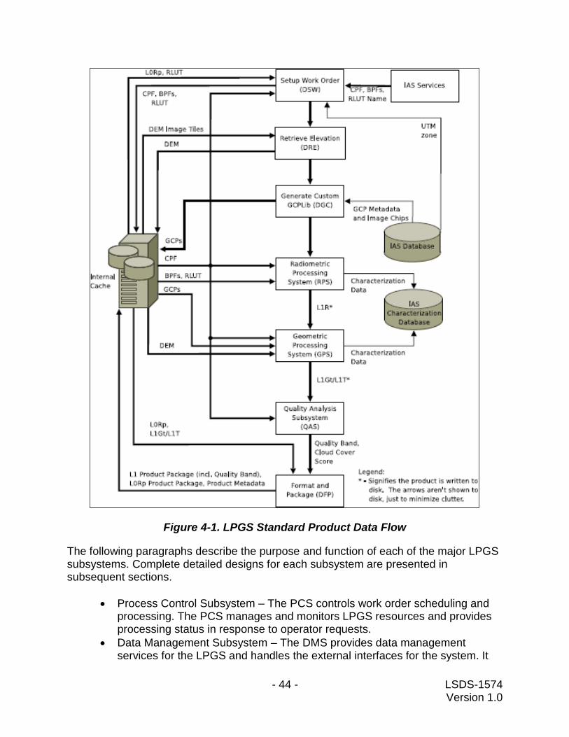
- 44 - LSDS-1574 Version 1.0

Figure 4-1. LPGS Standard Product Data Flow

The following paragraphs describe the purpose and function of each of the major LPGS subsystems. Complete detailed designs for each subsystem are presented in subsequent sections.

Process Control Subsystem – The PCS controls work order scheduling and processing. The PCS manages and monitors LPGS resources and provides processing status in response to operator requests.

Data Management Subsystem – The DMS provides data management services for the LPGS and handles the external interfaces for the system. It

- 45 - LSDS-1574 Version 1.0

provides tools for formatting and packaging products. The DMS also maintains LPGS disk space and populates temporary storage with data from ingested files.

Radiometric Processing Subsystem – The RPS converts the brightness of the L0R image pixels to absolute radiance in preparation for geometric correction. The RPS performs radiometric characterization of L0R images by locating radiometric artifacts in images. The RPS provides the results of characterizations performed to the IAS characterization database. The RPS corrects radiometric artifacts and converts the image to radiance.

Geometric Processing Subsystem – The GPS creates L1 geometrically corrected imagery (L1G) from L1R products. The geometrically corrected products can be systematic terrain corrected (L1Gt) or precision terrain corrected products (L1T). The GPS provides the results of characterizations performed to the IAS characterization database. The GPS generates a satellite model, prepares a resampling grid, and resamples the data to create a L1Gt or L1T product. The GPS performs sophisticated satellite geometric correction to create the image according the map projection and orientation specified for the L1 standard product.

Quality Assessment Subsystem – The QAS performs cloud cover assessment and generates the product quality band. The QAS provides tools for visual inspection of images where a problem has been encountered creating the product.

User Interface – The UI provides the Graphical User Interface (GUI) for the LPGS operator and the Anomaly Analysis Subsystem (AAS). It allows the operator to monitor the status of work orders and track processing anomalies.

4.1.3 Ancillary Data

The Landsat 8 OLI and TIRS geometric correction algorithms are applied to the wideband (data contained in Level 0R (raw) or 1R (radiometrically corrected) products. Some of these algorithms also require additional ancillary input data sets. These include:

1. Ancillary data from spacecraft & Space Inertial Reference Unit (SIRU: provides attitude information for the spacecraft)

2. Ground control/reference images for geometric test sites - used in precision correction, geodetic accuracy assessment, and geometric calibration algorithms.

3. Digital elevation data for geometric test sites - used in terrain correction and geometric calibration.

4. Pre-launch ground calibration results including band/detector placement and timing, and attitude sensor data transfer functions (gyro and ADS), to be used in the generation of the initial Calibration Parameter File.

5. Earth parameters including: static Earth model parameters (e.g., ellipsoid axes, gravity constants) and dynamic Earth model parameters (e.g., polar wander offsets, UT1-UTC time corrections) - used in systematic model creation and incorporated into the Calibration Parameter File.

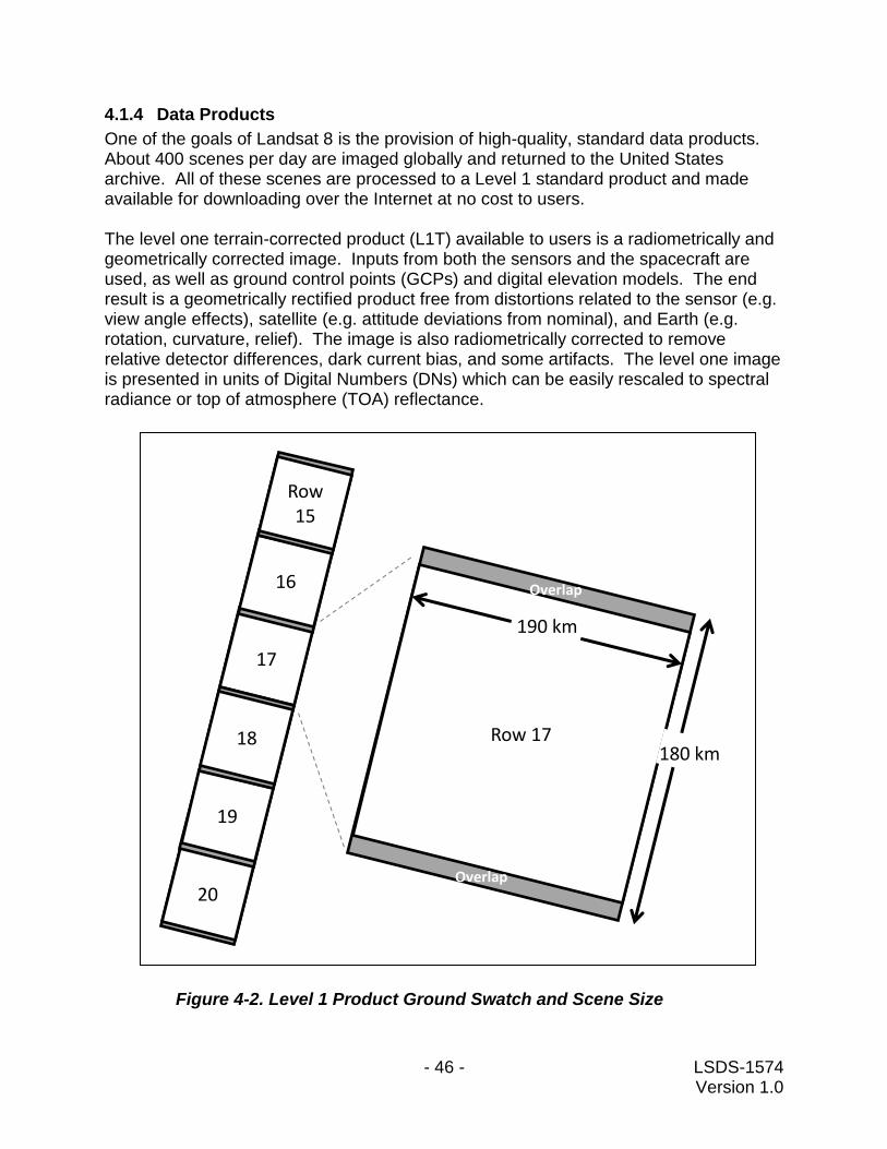
- 46 - LSDS-1574 Version 1.0

4.1.4 Data Products

One of the goals of Landsat 8 is the provision of high-quality, standard data products. About 400 scenes per day are imaged globally and returned to the United States archive. All of these scenes are processed to a Level 1 standard product and made available for downloading over the Internet at no cost to users. The level one terrain-corrected product (L1T) available to users is a radiometrically and geometrically corrected image. Inputs from both the sensors and the spacecraft are used, as well as ground control points (GCPs) and digital elevation models. The end result is a geometrically rectified product free from distortions related to the sensor (e.g. view angle effects), satellite (e.g. attitude deviations from nominal), and Earth (e.g. rotation, curvature, relief). The image is also radiometrically corrected to remove relative detector differences, dark current bias, and some artifacts. The level one image is presented in units of Digital Numbers (DNs) which can be easily rescaled to spectral radiance or top of atmosphere (TOA) reflectance.

Row 17

190 km

180 km

17

16

Row

15

20

19

18

Overlap

Overlap

Figure 4-2. Level 1 Product Ground Swatch and Scene Size

- 47 - LSDS-1574 Version 1.0

4.1.4.1 Product Components

A complete level 1 product consists of 13 files: The 11 band images, a product specific metadata file, and a Quality Assessment (QA) image. The image files are all 16-bit GeoTIFF images. The OLI bands are bands 1-9. The TIRS bands are designated as bands 10 and 11. The QA image is a 16-bit mask, which marks clouds, fill data, and some land cover types. A full description of the Landsat 8 QA mask is given in Section 5.4. The metadata (MTL) file contains identifying parameters for the scene along with the spatial extent of the scene and the processing parameters used to generate the level 1 product. It is a human-readable text file in Object Definition Language (ODL) format.

4.1.4.2 Product Format

The product delivered to Landsat 8 data users is packaged as Geographic tagged image file format (GeoTIFF), a standard, public-domain image format based on Adobe's TIFF, is a self-describing format developed to exchange raster images. The GeoTIFF format includes geographic or cartographic information embedded within the imagery that can be used to position the image in a geographic information display. Each Landsat 8 band is presented as a 16-bit grayscale image. Specifically, GeoTIFF defines a set of TIFF tags, which describe cartographic and geodetic information associated with geographic TIFF imagery. GeoTIFF is a means for tying a raster image to a known model space or map projection and for describing those projections. A metadata format provides geographic information to associate with the image data. However, the TIFF file structure allows both the metadata and the image data to be encoded into the same file. For details on GeoTIFF format, please download the GeoTIFF Format Specification (PDF) or visit this web site: http://trac.osgeo.org/geotiff/.

4.1.4.3 Cloud Cover Assessment

The Landsat 8 Cloud Cover Assessment (CCA) system uses multiple algorithms to detect clouds in scene data. Each CCA algorithm creates its own pixel mask that labels clouds, cirrus, and other classification types. The separate pixel masks are then merged together into the final level 1 quality band. The separate masks are merged together via a weighted voting mechanism. Each algorithm is assigned weights for every class (cloud, cirrus, water, and snow/ice), which indicates how accurate that algorithm is expected to be when classifying that type of target. These weights are defined in the CPF. Then for each pixel, the confidence value in each mask is used to sum the algorithm weights together:

N

j

kj

k

Whigh

1

,

0 otherwise

0.65 C if kj,

http://trac.osgeo.org/geotiff/

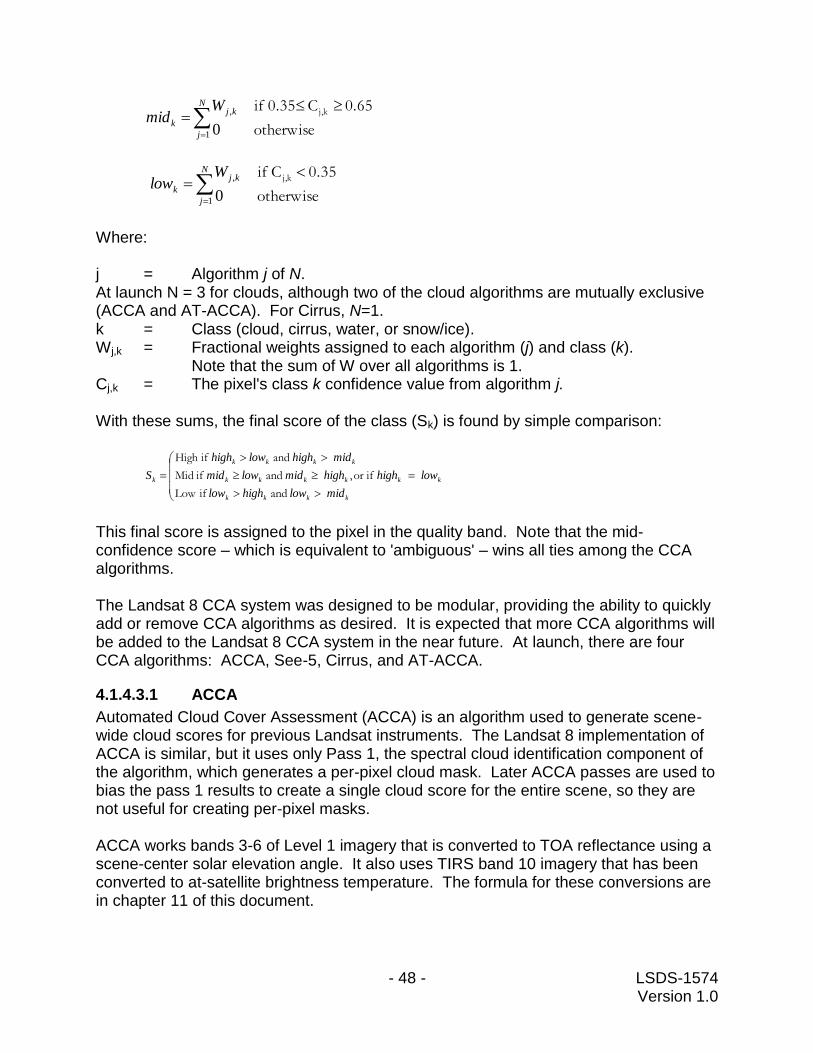
- 48 - LSDS-1574 Version 1.0

Where: j = Algorithm j of N. At launch N = 3 for clouds, although two of the cloud algorithms are mutually exclusive (ACCA and AT-ACCA). For Cirrus, N=1. k = Class (cloud, cirrus, water, or snow/ice). Wj,k = Fractional weights assigned to each algorithm (j) and class (k). Note that the sum of W over all algorithms is 1. Cj,k = The pixel's class k confidence value from algorithm j. With these sums, the final score of the class (Sk) is found by simple comparison:

This final score is assigned to the pixel in the quality band. Note that the mid-confidence score – which is equivalent to 'ambiguous' – wins all ties among the CCA algorithms. The Landsat 8 CCA system was designed to be modular, providing the ability to quickly add or remove CCA algorithms as desired. It is expected that more CCA algorithms will be added to the Landsat 8 CCA system in the near future. At launch, there are four CCA algorithms: ACCA, See-5, Cirrus, and AT-ACCA.

4.1.4.3.1 ACCA

Automated Cloud Cover Assessment (ACCA) is an algorithm used to generate scene-wide cloud scores for previous Landsat instruments. The Landsat 8 implementation of ACCA is similar, but it uses only Pass 1, the spectral cloud identification component of the algorithm, which generates a per-pixel cloud mask. Later ACCA passes are used to bias the pass 1 results to create a single cloud score for the entire scene, so they are not useful for creating per-pixel masks. ACCA works bands 3-6 of Level 1 imagery that is converted to TOA reflectance using a scene-center solar elevation angle. It also uses TIRS band 10 imagery that has been converted to at-satellite brightness temperature. The formula for these conversions are in chapter 11 of this document.

N

j

kj

k

Wmid

1

,

0 otherwise

0.65 C 0.35 if kj,

N

j

kj

k

Wlow

1

,

0 otherwise

0.35 C if kj,

kkkk

kkkkkk

kkkk

k

midlowhighlow

low high highmidlowmid

midhighlowhigh

S

and Low if

or if, and ifMid

and ifHigh

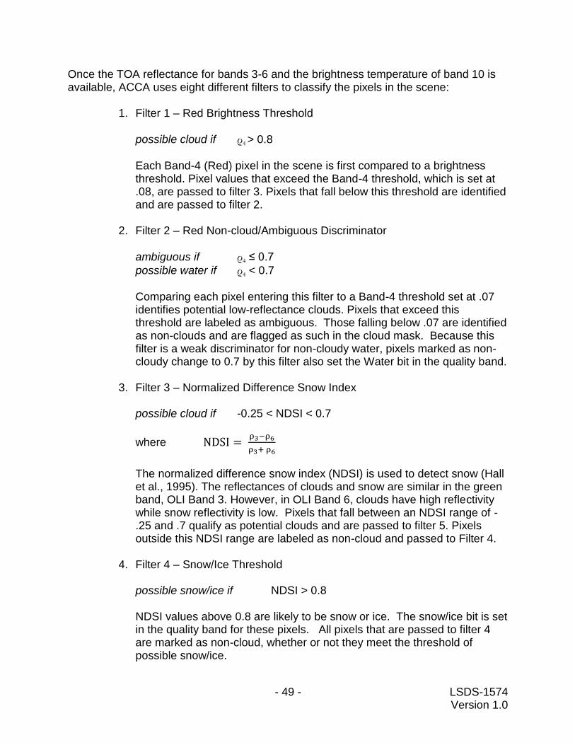
- 49 - LSDS-1574 Version 1.0

Once the TOA reflectance for bands 3-6 and the brightness temperature of band 10 is available, ACCA uses eight different filters to classify the pixels in the scene:

1. Filter 1 – Red Brightness Threshold

possible cloud if ρ4 > 0.8

Each Band-4 (Red) pixel in the scene is first compared to a brightness threshold. Pixel values that exceed the Band-4 threshold, which is set at .08, are passed to filter 3. Pixels that fall below this threshold are identified and are passed to filter 2.

2. Filter 2 – Red Non-cloud/Ambiguous Discriminator

ambiguous if ρ4 ≤ 0.7

possible water if ρ4 < 0.7

Comparing each pixel entering this filter to a Band-4 threshold set at .07 identifies potential low-reflectance clouds. Pixels that exceed this threshold are labeled as ambiguous. Those falling below .07 are identified as non-clouds and are flagged as such in the cloud mask. Because this filter is a weak discriminator for non-cloudy water, pixels marked as non-cloudy change to 0.7 by this filter also set the Water bit in the quality band.

3. Filter 3 – Normalized Difference Snow Index

possible cloud if -0.25 < NDSI < 0.7

where NDSI = ρ3−ρ6

ρ3+ ρ6

The normalized difference snow index (NDSI) is used to detect snow (Hall et al., 1995). The reflectances of clouds and snow are similar in the green band, OLI Band 3. However, in OLI Band 6, clouds have high reflectivity while snow reflectivity is low. Pixels that fall between an NDSI range of -.25 and .7 qualify as potential clouds and are passed to filter 5. Pixels outside this NDSI range are labeled as non-cloud and passed to Filter 4.

4. Filter 4 – Snow/Ice Threshold

possible snow/ice if NDSI > 0.8

NDSI values above 0.8 are likely to be snow or ice. The snow/ice bit is set in the quality band for these pixels. All pixels that are passed to filter 4 are marked as non-cloud, whether or not they meet the threshold of possible snow/ice.

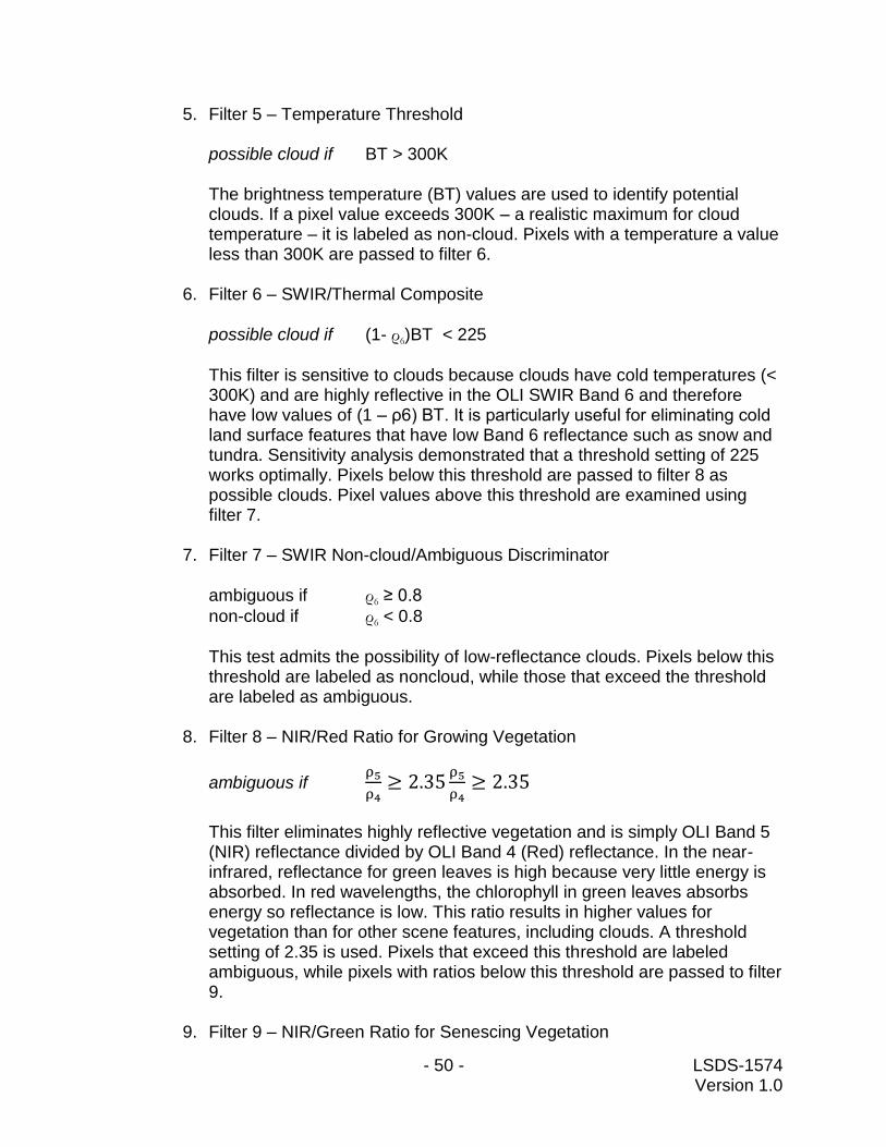
- 50 - LSDS-1574 Version 1.0

5. Filter 5 – Temperature Threshold

possible cloud if BT > 300K

The brightness temperature (BT) values are used to identify potential clouds. If a pixel value exceeds 300K – a realistic maximum for cloud temperature – it is labeled as non-cloud. Pixels with a temperature a value less than 300K are passed to filter 6.

6. Filter 6 – SWIR/Thermal Composite

possible cloud if (1- ρ6)BT < 225

This filter is sensitive to clouds because clouds have cold temperatures (< 300K) and are highly reflective in the OLI SWIR Band 6 and therefore have low values of (1 – ρ6) BT. It is particularly useful for eliminating cold land surface features that have low Band 6 reflectance such as snow and tundra. Sensitivity analysis demonstrated that a threshold setting of 225 works optimally. Pixels below this threshold are passed to filter 8 as possible clouds. Pixel values above this threshold are examined using filter 7.

7. Filter 7 – SWIR Non-cloud/Ambiguous Discriminator

ambiguous if ρ6 ≥ 0.8

non-cloud if ρ6 < 0.8

This test admits the possibility of low-reflectance clouds. Pixels below this threshold are labeled as noncloud, while those that exceed the threshold are labeled as ambiguous.

8. Filter 8 – NIR/Red Ratio for Growing Vegetation

ambiguous if ρ5

ρ4≥ 2.35

ρ5

ρ4≥ 2.35

This filter eliminates highly reflective vegetation and is simply OLI Band 5 (NIR) reflectance divided by OLI Band 4 (Red) reflectance. In the near-infrared, reflectance for green leaves is high because very little energy is absorbed. In red wavelengths, the chlorophyll in green leaves absorbs energy so reflectance is low. This ratio results in higher values for vegetation than for other scene features, including clouds. A threshold setting of 2.35 is used. Pixels that exceed this threshold are labeled ambiguous, while pixels with ratios below this threshold are passed to filter 9.

9. Filter 9 – NIR/Green Ratio for Senescing Vegetation

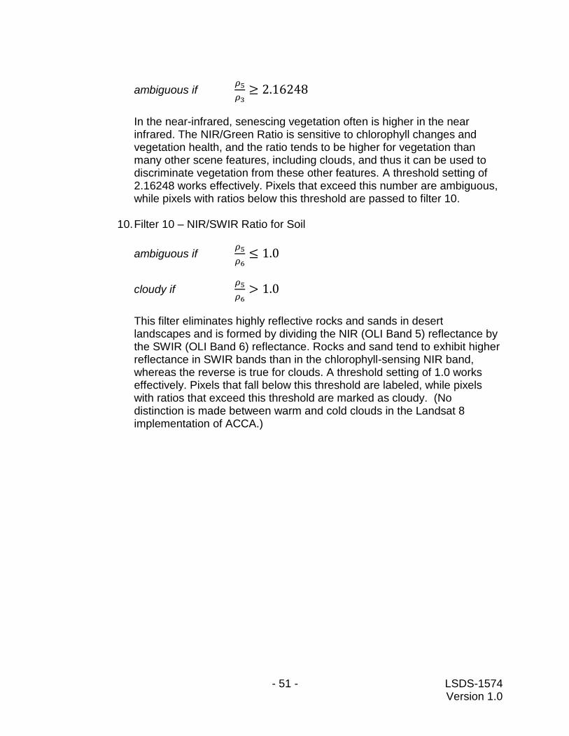
- 51 - LSDS-1574 Version 1.0

ambiguous if 𝜌5

𝜌3≥ 2.16248

In the near-infrared, senescing vegetation often is higher in the near infrared. The NIR/Green Ratio is sensitive to chlorophyll changes and vegetation health, and the ratio tends to be higher for vegetation than many other scene features, including clouds, and thus it can be used to discriminate vegetation from these other features. A threshold setting of 2.16248 works effectively. Pixels that exceed this number are ambiguous, while pixels with ratios below this threshold are passed to filter 10.

10. Filter 10 – NIR/SWIR Ratio for Soil

ambiguous if 𝜌5

𝜌6≤ 1.0

cloudy if 𝜌5

𝜌6> 1.0

This filter eliminates highly reflective rocks and sands in desert landscapes and is formed by dividing the NIR (OLI Band 5) reflectance by the SWIR (OLI Band 6) reflectance. Rocks and sand tend to exhibit higher reflectance in SWIR bands than in the chlorophyll-sensing NIR band, whereas the reverse is true for clouds. A threshold setting of 1.0 works effectively. Pixels that fall below this threshold are labeled, while pixels with ratios that exceed this threshold are marked as cloudy. (No distinction is made between warm and cold clouds in the Landsat 8 implementation of ACCA.)

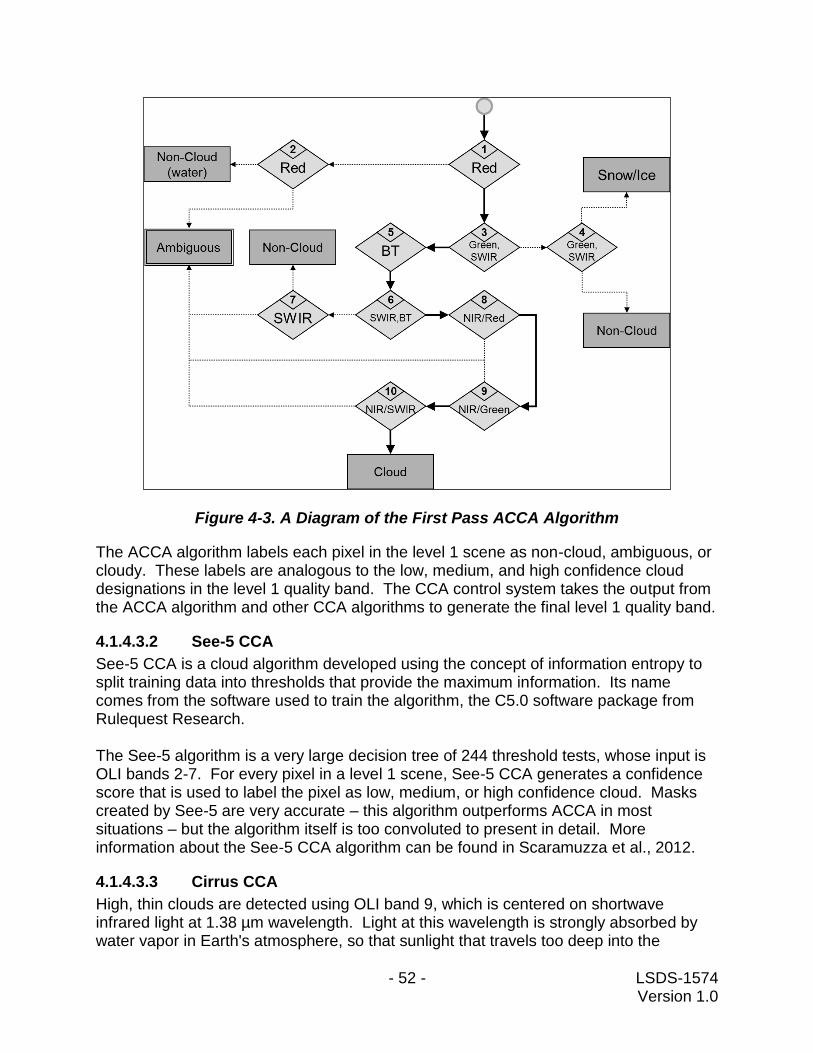
- 52 - LSDS-1574 Version 1.0

Figure 4-3. A Diagram of the First Pass ACCA Algorithm

The ACCA algorithm labels each pixel in the level 1 scene as non-cloud, ambiguous, or cloudy. These labels are analogous to the low, medium, and high confidence cloud designations in the level 1 quality band. The CCA control system takes the output from the ACCA algorithm and other CCA algorithms to generate the final level 1 quality band.

4.1.4.3.2 See-5 CCA

See-5 CCA is a cloud algorithm developed using the concept of information entropy to split training data into thresholds that provide the maximum information. Its name comes from the software used to train the algorithm, the C5.0 software package from Rulequest Research. The See-5 algorithm is a very large decision tree of 244 threshold tests, whose input is OLI bands 2-7. For every pixel in a level 1 scene, See-5 CCA generates a confidence score that is used to label the pixel as low, medium, or high confidence cloud. Masks created by See-5 are very accurate – this algorithm outperforms ACCA in most situations – but the algorithm itself is too convoluted to present in detail. More information about the See-5 CCA algorithm can be found in Scaramuzza et al., 2012.

4.1.4.3.3 Cirrus CCA

High, thin clouds are detected using OLI band 9, which is centered on shortwave infrared light at 1.38 µm wavelength. Light at this wavelength is strongly absorbed by water vapor in Earth's atmosphere, so that sunlight that travels too deep into the

- 53 - LSDS-1574 Version 1.0

atmosphere cannot reflect back to the satellite. Cirrus clouds are high in the atmosphere and thus above most of the water vapor, so they are strong reflectors of this 1.38 µm radiation. The Landsat 8 Cirrus CCA algorithm is a simple threshold test for reflectance in OLI band 9. The threshold is set in the CPF; the at-launch threshold is 2% reflectance. Any object with greater reflectance in band 9 is marked as possible cirrus. Cirrus if: ρ9 > Tcirrus where: ρ9 = TOA reflectance in OLI band 9.

(Note that this is calculated from the level 1G product using a scene-center solar elevation angle.)

Tcirrus = Cirrus threshold from the CPF. (0.02 at launch) This test is very permissive, and it detects false positives over high-altitude arid regions and over the poles, where the air is very cold and dry. The cirrus test is very accurate over low to moderate elevation areas in non-polar regions.

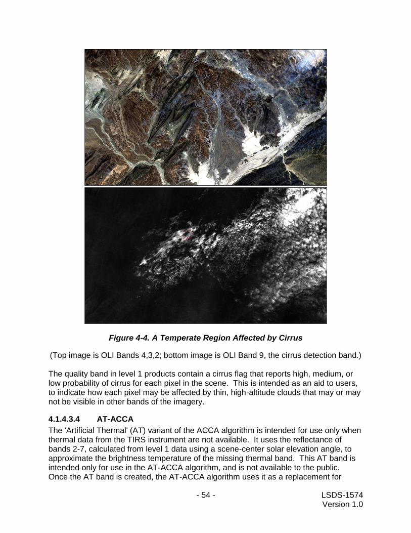
- 54 - LSDS-1574 Version 1.0

Figure 4-4. A Temperate Region Affected by Cirrus

(Top image is OLI Bands 4,3,2; bottom image is OLI Band 9, the cirrus detection band.) The quality band in level 1 products contain a cirrus flag that reports high, medium, or low probability of cirrus for each pixel in the scene. This is intended as an aid to users, to indicate how each pixel may be affected by thin, high-altitude clouds that may or may not be visible in other bands of the imagery.

4.1.4.3.4 AT-ACCA

The 'Artificial Thermal' (AT) variant of the ACCA algorithm is intended for use only when thermal data from the TIRS instrument are not available. It uses the reflectance of bands 2-7, calculated from level 1 data using a scene-center solar elevation angle, to approximate the brightness temperature of the missing thermal band. This AT band is intended only for use in the AT-ACCA algorithm, and is not available to the public. Once the AT band is created, the AT-ACCA algorithm uses it as a replacement for

- 55 - LSDS-1574 Version 1.0

brightness temperature (BT) in the same threshold filters as the normal ACCA algorithm. Note that ACCA and AT-ACCA are never run together; if a thermal band exists, ACCA is run, if no thermal band exists then AT-ACCA is used. A large number of pixels are labeled ambiguous by the filters in the AT-ACCA algorithm. To reduce the number of ambiguous pixels, a second pass is made using an additional suite of disambiguation threshold tests. These disambiguation tests are only applied to pixels labeled ambiguous by the AT-ACCA. The tests are simple thresholds that are statistically unlikely to indicate clouds among data normally marked as ambiguous by ACCA. If a pixel passes any two of these tests, it is labeled as non-cloud. Pixels that pass only one or zero tests remain ambiguous. Similar to the ACCA algorithm, the AT-ACCA's labels of non-cloud, ambiguous, and cloud pixels are analogous to the low, medium, and high confidence cloud designations in the level 1 quality band. Full details on the AT band, the AT-ACCA algorithm, and the AT-ACCA disambiguation tests can be found in Scaramuzza et al., 2012.

4.1.5 Calculation of Scene Quality

The quality algorithm is calculated by the following two formulas: SIQS = 9 - [ SNF/ANF * ( NDF / DFBP + NCF / CFBP)] IIQS = 9 - [(NDF/DFBP + NCF/CFBP) Where: SIQS = Scene Image Quality Score IIQS = Interval Image Quality Score SNF = Standard number of video frames in a scene [7001 for OLI, 2621 for TIRS] ANF = Actual number of frames in the scene / interval NDF = Number of dropped frames in the scene / interval DFBP = Dropped Frame Break Point: dropped frame count at which the quality score

drops by one point. [2] NCF = Number of video frame CRC failures in the scene / interval CFBP = CRC Failures Break Point: Video frame CRC failure count at which the quality

score drops by one point. [100] Numbers in brackets are configurable. If changed, the quality algorithm version is updated and the new values documented Image_Quality_OLI Values: 0–9, where 9 = Best. 0 = Worst -1 = quality not calculated or assessed.

- 56 - LSDS-1574 Version 1.0

Image_Quality_TIRS Values: 0–9, where 9 = Best. 0 = Worst. -1 = quality not calculated or assessed.

4.2 Level 1 Product Description

4.2.1 Science Data Content and Format

The Landsat 8 instruments, OLI and TIRS, represent an evolutionary advance in technology. OLI builds upon Landsat heritage and technologies demonstrated by the Advanced Land Imager (ALI). As such, OLI is a push-broom sensor with a four mirror telescope and uses 12-bit quantization. The OLI collects 30 meter data for visible, near infrared, and short wave infrared spectral bands as well as provides for a 15 meter panchromatic band. New with OLI is the addition of a 30 meter deep blue Coastal Aerosol band (Band 1) for coastal water and aerosol studies and a 30 meter Cirrus band (Band 9) for cirrus cloud detection. Additionally, the bandwidth has been refined (narrowed) for six of the heritage bands. The TIRS instrument collects data for two narrow spectral bands in the thermal region, formerly covered on previous Landsat instruments by one wide spectral band. Although TIRS is a separate instrument, the 100 meter TIRS data are registered to the OLI data in order to create radiometrically, geometrically, and terrain-corrected 12-bit data products. These sensors both provide improved signal-to-noise (SNR) radiometric performance quantized over a 12-bit dynamic range. This translates into 4096 potential grey levels in an image compared with only 256 grey levels in previous 8-bit instruments. Additionally, improved signal-to-noise performance enables better characterization of land cover state and condition.

4.2.1.1 Science Data Content

In addition to the Table 2-1 in Section 2, the following graphic compares Landast-8 spectral bands and wavelength to that of Landsat-7 ETM+.

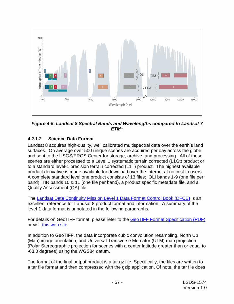
- 57 - LSDS-1574 Version 1.0

Figure 4-5. Landsat 8 Spectral Bands and Wavelengths compared to Landsat 7 ETM+

4.2.1.2 Science Data Format

Landsat 8 acquires high-quality, well calibrated multispectral data over the earth’s land surfaces. On average over 500 unique scenes are acquired per day across the globe and sent to the USGS/EROS Center for storage, archive, and processing. All of these scenes are either processed to a Level 1 systematic terrain corrected (L1Gt) product or to a standard level-1 precision terrain corrected (L1T) product. The highest available product derivative is made available for download over the Internet at no cost to users. A complete standard level one product consists of 13 files: OLI bands 1-9 (one file per band), TIR bands 10 & 11 (one file per band), a product specific metadata file, and a Quality Assessment (QA) file. The Landsat Data Continuity Mission Level 1 Data Format Control Book (DFCB) is an excellent reference for Landsat 8 product format and information. A summary of the level-1 data format is annotated in the following paragraphs. For details on GeoTIFF format, please refer to the GeoTIFF Format Specification (PDF) or visit this web site. In addition to GeoTIFF, the data incorporate cubic convolution resampling, North Up (Map) image orientation, and Universal Transverse Mercator (UTM) map projection (Polar Stereographic projection for scenes with a center latitude greater than or equal to -63.0 degrees) using the WGS84 datum. The format of the final output product is a tar.gz file. Specifically, the files are written to a tar file format and then compressed with the gzip application. Of note, the tar file does

http://landsat.usgs.gov/documents/LDCM-DFCB-004.pdf

http://landsathandbook.gsfc.nasa.gov/pdfs/geotiff_spec.pdf

http://trac.osgeo.org/geotiff/

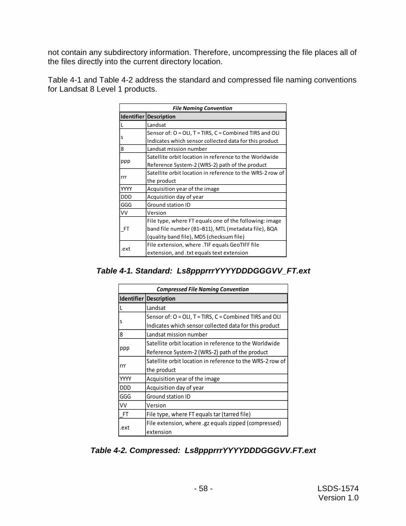
- 58 - LSDS-1574 Version 1.0

not contain any subdirectory information. Therefore, uncompressing the file places all of the files directly into the current directory location. Table 4-1 and Table 4-2 address the standard and compressed file naming conventions for Landsat 8 Level 1 products.

Table 4-1. Standard: Ls8ppprrrYYYYDDDGGGVV_FT.ext

Table 4-2. Compressed: Ls8ppprrrYYYYDDDGGGVV.FT.ext

Identifier Description

L Landsat

s Sensor of: O = OLI, T = TIRS, C = Combined TIRS and OLI

Indicates which sensor collected data for this product

8 Landsat mission number

ppp Satellite orbit location in reference to the Worldwide

Reference System-2 (WRS-2) path of the product

rrr Satellite orbit location in reference to the WRS-2 row of

the product

YYYY Acquisition year of the image

DDD Acquisition day of year

GGG Ground station ID

VV Version

_FT

File type, where FT equals one of the following: image

band file number (B1–B11), MTL (metadata file), BQA

(quality band file), MD5 (checksum file)

.ext File extension, where .TIF equals GeoTIFF file

extension, and .txt equals text extension

File Naming Convention

Identifier Description

L Landsat

s Sensor of: O = OLI, T = TIRS, C = Combined TIRS and OLI

Indicates which sensor collected data for this product

8 Landsat mission number

ppp Satellite orbit location in reference to the Worldwide

Reference System-2 (WRS-2) path of the product

rrr Satellite orbit location in reference to the WRS-2 row of

the product

YYYY Acquisition year of the image

DDD Acquisition day of year

GGG Ground station ID

VV Version

_FT File type, where FT equals tar (tarred file)

.ext File extension, where .gz equals zipped (compressed)

extension

Compressed File Naming Convention

- 59 - LSDS-1574 Version 1.0

4.2.2 Metadata Content and Format

The metadata (MTL) file is created during product generation and contains information specific to the level one product ordered. The MTL file contains identifying parameters for the scene along with the spatial extent of the scene and the processing parameters used to generate the level 1 product. It is a human-readable text file in Object Definition Language (ODL) format. The complete description of the metadata file is provided in the Landsat Data Continuity Mission Level 1 Data Format Control Book (DFCB). In general, the MTL file includes the following parameters:

Unique Landsat scene identifier

WRS path and row information

Scene Center Time of the date the image was acquired

Corner longitude and latitude in degrees and map projection values in meters

Reflective, thermal, and panchromatic band lines and samples

File names included

Image attributes including cloud cover, sun azimuth & elevation, number of ground control points used

Band minimum and maximum reflectance and radiance rescaling

4.2.3 Quality Assurance Band

The Quality Assessment (QA) Band file contains quality statistics gathered from the image data and cloud mask information for the scene. The QA file is a 16-bit image with the same dimensions as the standard L1T scene. Bits are allocated for some artifacts that are distinguishable after systematic correction (Level-1G) stage of processing. The first bit (bit 0) is the least significant. A full description of the Landsat 8 QA band is given in Section 5.4. Used effectively, QA bits improve the integrity of science investigations by indicating which pixels might be affected by instrument artifacts or subject to cloud contamination. For example, NDVI calculated over pixels containing clouds will show anomalous values. If such pixels were included in a phenology study, the results might not show the true characteristics of seasonal vegetation growth. Cloud contaminated pixels will lower NDVI values, and measures like the timing of ‘green up’ or peak maturity would appear later than they actually occurred. A worse consequence would be that the reported reduction of vegetation growth would be taken as an indicator of environmental change, potentially prompting unnecessary land management policies or practices. Rigorous science applications seeking to optimize the value of pixels used in a study will find QA bits useful as a first level indicator of certain conditions. Otherwise, users are advised that this file contains information that can be easily misinterpreted and it is not recommended for general use. Robust image processing software capable of handling 16-bit data is necessary to compute statistics of the number of pixels containing each of the designated bits.


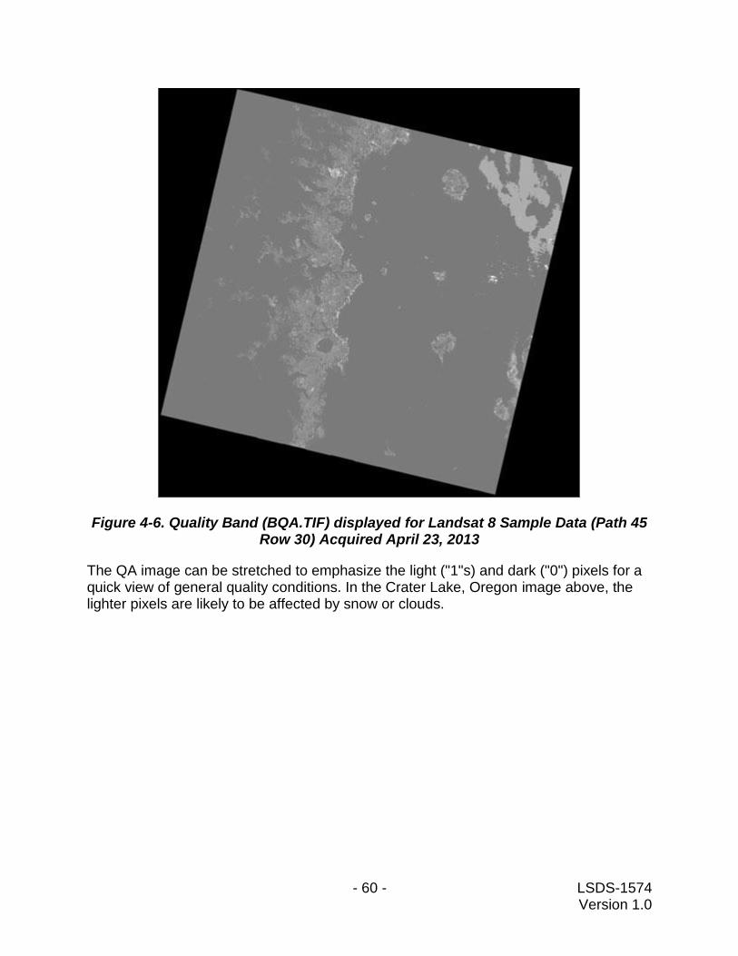
- 60 - LSDS-1574 Version 1.0

Figure 4-6. Quality Band (BQA.TIF) displayed for Landsat 8 Sample Data (Path 45 Row 30) Acquired April 23, 2013

The QA image can be stretched to emphasize the light ("1"s) and dark ("0") pixels for a quick view of general quality conditions. In the Crater Lake, Oregon image above, the lighter pixels are likely to be affected by snow or clouds.

- 61 - LSDS-1574 Version 1.0

Section 5 Conversion of DNs to Physical Units

5.1 OLI and TIRS at Sensor Spectral Radiance

Images are processed in units of absolute radiance using 32-bit floating point calculations. These values are then converted to 16-bit integer values in the finished level 1 product. These values can then be converted to spectral radiance using the radiance scaling factors provided in the metadata file:

Lλ = ML*Qcal + AL where: Lλ = Spectral radiance (W/(m2 * sr * μm)) ML = Radiance multiplicative scaling factor for the band (RADIANCE_MULT_BAND_n from the metadata). AL = Radiance additive scaling factor for the band (RADIANCE_ADD_BAND_n from the metadata). Qcal = Level 1 pixel value in DN

5.2 OLI Top of Atmosphere Reflectance

Similar to the conversion to radiance, the 16-bit integer values in the level 1 product can also be converted to Top of Atmosphere (TOA) reflectance. The following equation is used to convert level 1 DN values to TOA reflectance:

ρλ' = M*Qcal + A where: ρλ' = Top-of-Atmosphere Planetary Spectral Reflectance, without correction for solar angle. (Unitless)

M = Reflectance multiplicative scaling factor for the band (REFLECTANCEW_MULT_BAND_n from the metadata).

A = Reflectance additive scaling factor for the band (REFLECTANCE_ADD_BAND_N from the metadata). Qcal = Level 1 pixel value in DN Note that ρλ' is not true TOA Reflectance, because it does not contain a correction for the solar elevation angle. This correction factor is left out of the level 1 scaling at the users' request; some users are content with the scene-center solar elevation angle in the metadata, while others prefer to calculate their own per-pixel solar elevation angle across the entire scene. Once a solar elevation angle is chosen, the conversion to true TOA Reflectance is:

ρλ=

ρλ'

sin(θ)

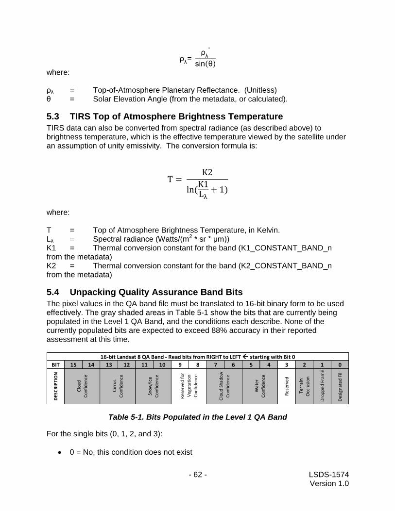
- 62 - LSDS-1574 Version 1.0

ρλ=

ρλ'

sin(θ)

where: ρλ = Top-of-Atmosphere Planetary Reflectance. (Unitless) θ = Solar Elevation Angle (from the metadata, or calculated).

5.3 TIRS Top of Atmosphere Brightness Temperature

TIRS data can also be converted from spectral radiance (as described above) to brightness temperature, which is the effective temperature viewed by the satellite under an assumption of unity emissivity. The conversion formula is:

T = K2

ln (K1Lλ

+ 1)

where: T = Top of Atmosphere Brightness Temperature, in Kelvin. Lλ = Spectral radiance (Watts/(m2 * sr * μm)) K1 = Thermal conversion constant for the band (K1_CONSTANT_BAND_n from the metadata) K2 = Thermal conversion constant for the band (K2_CONSTANT_BAND_n from the metadata)

5.4 Unpacking Quality Assurance Band Bits

The pixel values in the QA band file must be translated to 16-bit binary form to be used effectively. The gray shaded areas in Table 5-1 show the bits that are currently being populated in the Level 1 QA Band, and the conditions each describe. None of the currently populated bits are expected to exceed 88% accuracy in their reported assessment at this time.

Table 5-1. Bits Populated in the Level 1 QA Band

For the single bits (0, 1, 2, and 3):

0 = No, this condition does not exist

BIT 15 14 13 12 11 10 9 8 7 6 5 4 3 2 1 0

DES

CR

IPTI

ON

Res

erve

d

Terr

ain

Occ

lusi

on

Dro

pped

Fra

me

Des

igna

ted

Fill

16-bit Landsat 8 QA Band - Read bits from RIGHT to LEFT starting with Bit 0

Clo

ud

Con

fide

nce

Cir

rus

Con

fide

nce

Snow

/Ice

Con

fide

nce

Res

erve

d fo

r

Veg

etat

ion

Con

fide

nce

Clo

ud S

hado

w

Con

fide

nce

Wat

er

Con

fide

nce

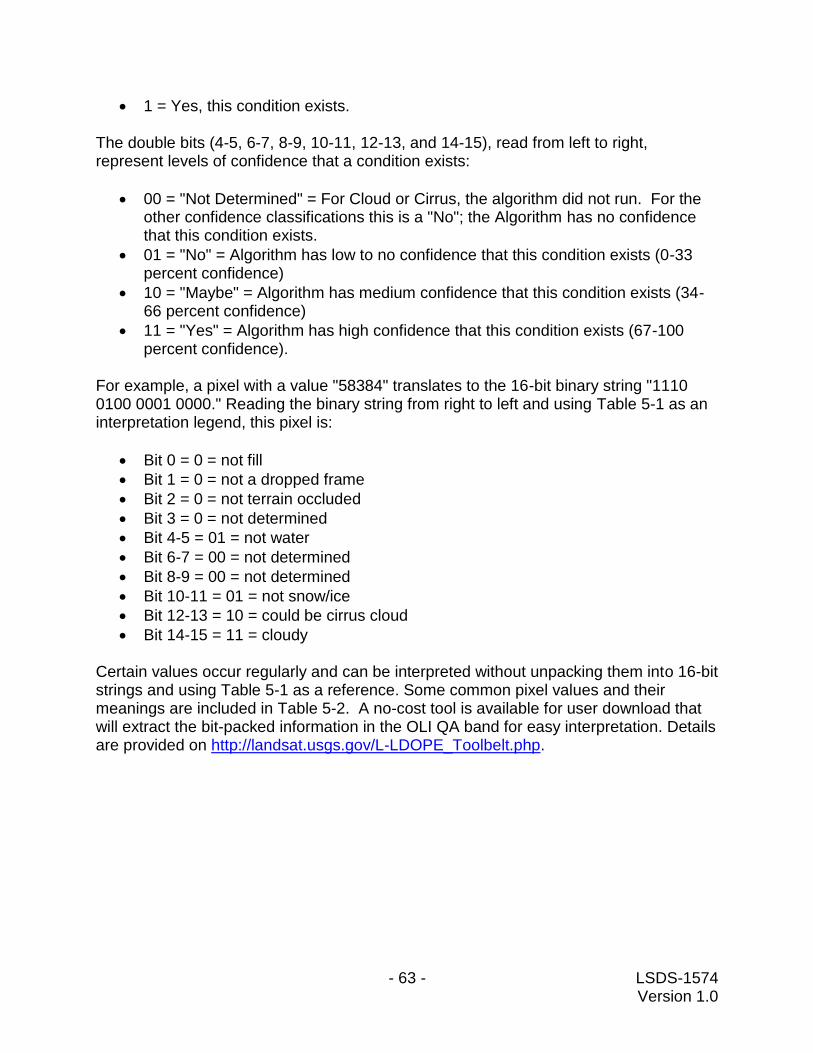
- 63 - LSDS-1574 Version 1.0

1 = Yes, this condition exists. The double bits (4-5, 6-7, 8-9, 10-11, 12-13, and 14-15), read from left to right, represent levels of confidence that a condition exists:

00 = "Not Determined" = For Cloud or Cirrus, the algorithm did not run. For the other confidence classifications this is a "No"; the Algorithm has no confidence that this condition exists.

01 = "No" = Algorithm has low to no confidence that this condition exists (0-33 percent confidence)

10 = "Maybe" = Algorithm has medium confidence that this condition exists (34-66 percent confidence)

11 = "Yes" = Algorithm has high confidence that this condition exists (67-100 percent confidence).

For example, a pixel with a value "58384" translates to the 16-bit binary string "1110 0100 0001 0000." Reading the binary string from right to left and using Table 5-1 as an interpretation legend, this pixel is:

Bit 0 = 0 = not fill

Bit 1 = 0 = not a dropped frame

Bit 2 = 0 = not terrain occluded

Bit 3 = 0 = not determined

Bit 4-5 = 01 = not water

Bit 6-7 = 00 = not determined

Bit 8-9 = 00 = not determined

Bit 10-11 = 01 = not snow/ice

Bit 12-13 = 10 = could be cirrus cloud

Bit 14-15 = 11 = cloudy Certain values occur regularly and can be interpreted without unpacking them into 16-bit strings and using Table 5-1 as a reference. Some common pixel values and their meanings are included in Table 5-2. A no-cost tool is available for user download that will extract the bit-packed information in the OLI QA band for easy interpretation. Details are provided on http://landsat.usgs.gov/L-LDOPE_Toolbelt.php.

http://landsat.usgs.gov/L-LDOPE_Toolbelt.php

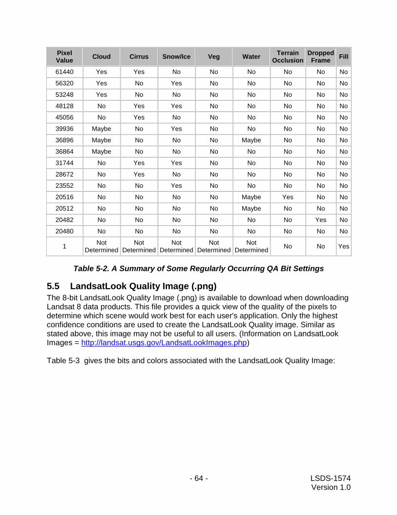
- 64 - LSDS-1574 Version 1.0

Pixel Value

Cloud Cirrus Snow/Ice Veg Water Terrain

Occlusion Dropped Frame

Fill

61440 Yes Yes No No No No No No

56320 Yes No Yes No No No No No

53248 Yes No No No No No No No

48128 No Yes Yes No No No No No

45056 No Yes No No No No No No

39936 Maybe No Yes No No No No No

36896 Maybe No No No Maybe No No No

36864 Maybe No No No No No No No

31744 No Yes Yes No No No No No

28672 No Yes No No No No No No

23552 No No Yes No No No No No

20516 No No No No Maybe Yes No No

20512 No No No No Maybe No No No

20482 No No No No No No Yes No

20480 No No No No No No No No

1 Not

Determined Not

Determined Not

Determined Not

Determined Not

Determined No No Yes

Table 5-2. A Summary of Some Regularly Occurring QA Bit Settings

5.5 LandsatLook Quality Image (.png)

The 8-bit LandsatLook Quality Image (.png) is available to download when downloading Landsat 8 data products. This file provides a quick view of the quality of the pixels to determine which scene would work best for each user's application. Only the highest confidence conditions are used to create the LandsatLook Quality image. Similar as stated above, this image may not be useful to all users. (Information on LandsatLook Images = http://landsat.usgs.gov/LandsatLookImages.php) Table 5-3 gives the bits and colors associated with the LandsatLook Quality Image:

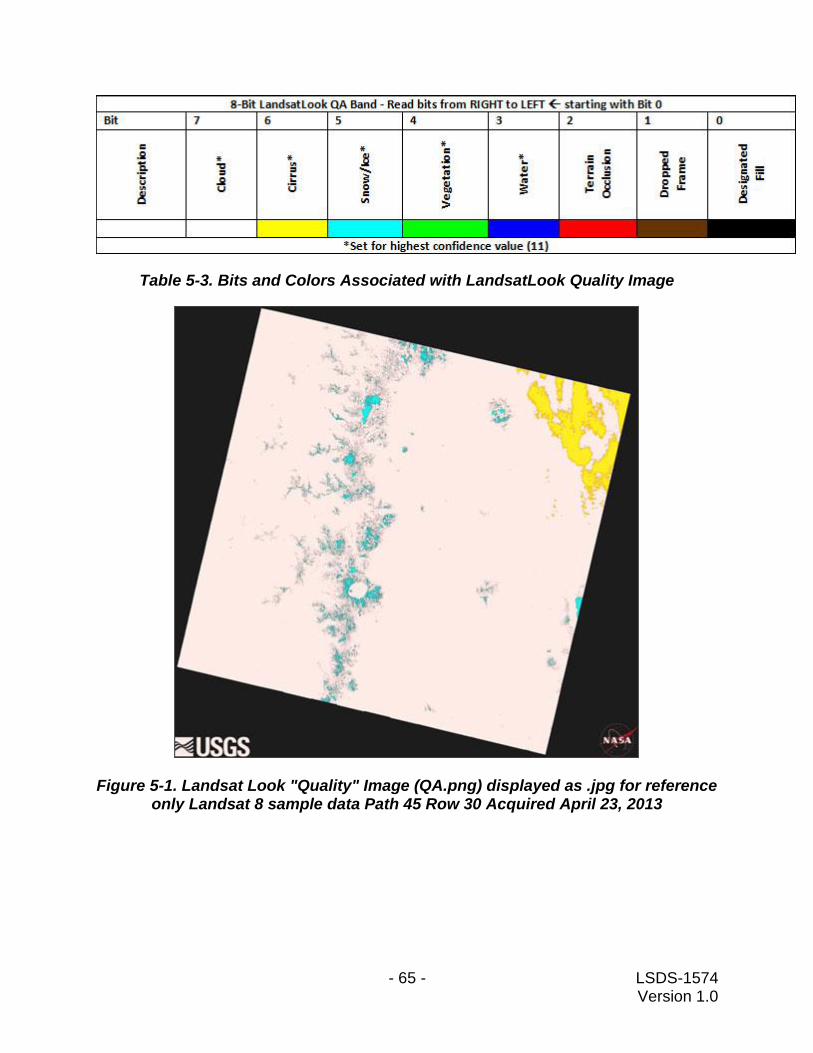
http://landsat.usgs.gov/LandsatLookImages.php

- 65 - LSDS-1574 Version 1.0

Table 5-3. Bits and Colors Associated with LandsatLook Quality Image

Figure 5-1. Landsat Look "Quality" Image (QA.png) displayed as .jpg for reference only Landsat 8 sample data Path 45 Row 30 Acquired April 23, 2013

- 66 - LSDS-1574 Version 1.0

Section 6 Data Search and Access

The USGS archive holds data collected by the Landsat suite of satellites, beginning with Landsat 1 in 1972. Over 500 Landsat 8 scenes are added to the USGS archives each day, and become available to all users for download at no charge using the sites described in this section. All Landsat data products are distributed via HTTPS access. Current Landsat 8 products available include:

LandsatLook “Natural Color” Image - a full-resolution, 3-band .jpg image (approximate size: 4.5 MB)

LandsatLook “Thermal” Image - a full-a resolution, thermal band 10 .jpg image (approximate size: 2.5 MB)

LandsatLook “Quality” Image - a full-resolution Quality Assessment band .png image (Approximate size: 2.5 MB)

LandsatLook Images with Geographic Reference - a bundle including the “Natural”, “Thermal”, and “Quality” full-resolution images, along with .wld and .xml files with geographic reference information (Approximate size: 9.0 MB)

Level 1 Data Product - a compressed file including all individual multispectral and/or thermal band and metadata files (Approximate size: 950 MB)

Details about Landsat 8 data products can be found on http://landsat.usgs.gov/landsat8.php. The following interfaces allow searching and downloading of Landsat 8 data held in the USGS Archives. The functionality of each differs; however, the data products are all delivered from the same location. Each interface includes a Help section to provide more details about step-by-step processes.

6.1 Earth Explorer (EE)

Earth Explorer (EE) is the primary search interface accessing aerial, mapping, elevation, and satellite data held in the USGS archives, including Landsat data products. A USGS Registered Login name is required to download data products. Some functions of the website will work only after a successful login. New users can register at https://earthexplorer.usgs.gov/register/. http://earthexplorer.usgs.gov

http://landsat.usgs.gov/about_mission_history.php

http://landsat.usgs.gov/landsat8.php

https://earthexplorer.usgs.gov/register/

http://earthexplorer.usgs.gov/

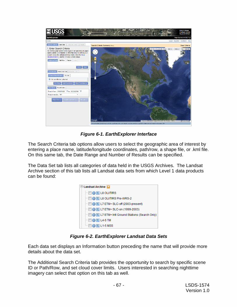
- 67 - LSDS-1574 Version 1.0

Figure 6-1. EarthExplorer Interface

The Search Criteria tab options allow users to select the geographic area of interest by entering a place name, latitude/longitude coordinates, path/row, a shape file, or .kml file. On this same tab, the Date Range and Number of Results can be specified. The Data Set tab lists all categories of data held in the USGS Archives. The Landsat Archive section of this tab lists all Landsat data sets from which Level 1 data products can be found:

Figure 6-2. EarthExplorer Landsat Data Sets

Each data set displays an Information button preceding the name that will provide more details about the data set. The Additional Search Criteria tab provides the opportunity to search by specific scene ID or Path/Row, and set cloud cover limits. Users interested in searching nighttime imagery can select that option on this tab as well.

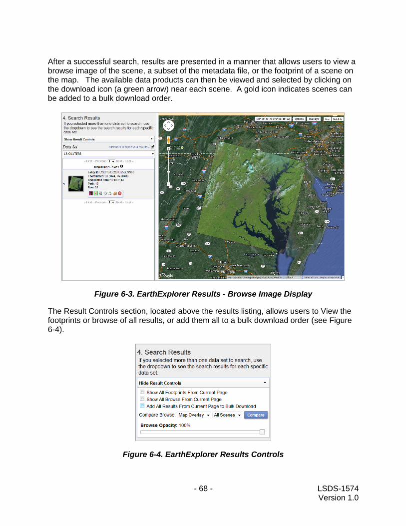
- 68 - LSDS-1574 Version 1.0

After a successful search, results are presented in a manner that allows users to view a browse image of the scene, a subset of the metadata file, or the footprint of a scene on the map. The available data products can then be viewed and selected by clicking on the download icon (a green arrow) near each scene. A gold icon indicates scenes can be added to a bulk download order.

Figure 6-3. EarthExplorer Results - Browse Image Display

The Result Controls section, located above the results listing, allows users to View the footprints or browse of all results, or add them all to a bulk download order (see Figure 6-4).

Figure 6-4. EarthExplorer Results Controls

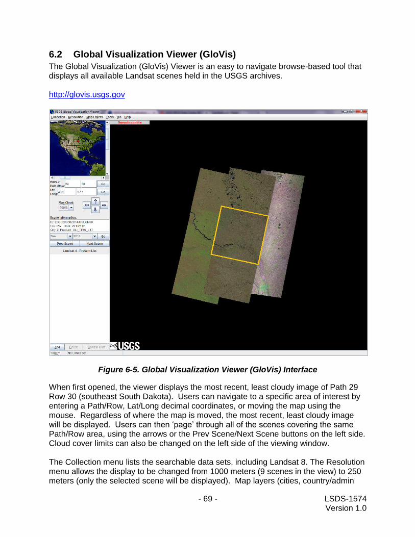
- 69 - LSDS-1574 Version 1.0

6.2 Global Visualization Viewer (GloVis)

The Global Visualization (GloVis) Viewer is an easy to navigate browse-based tool that displays all available Landsat scenes held in the USGS archives. http://glovis.usgs.gov

Figure 6-5. Global Visualization Viewer (GloVis) Interface

When first opened, the viewer displays the most recent, least cloudy image of Path 29 Row 30 (southeast South Dakota). Users can navigate to a specific area of interest by entering a Path/Row, Lat/Long decimal coordinates, or moving the map using the mouse. Regardless of where the map is moved, the most recent, least cloudy image will be displayed. Users can then ‘page’ through all of the scenes covering the same Path/Row area, using the arrows or the Prev Scene/Next Scene buttons on the left side. Cloud cover limits can also be changed on the left side of the viewing window. The Collection menu lists the searchable data sets, including Landsat 8. The Resolution menu allows the display to be changed from 1000 meters (9 scenes in the view) to 250 meters (only the selected scene will be displayed). Map layers (cities, country/admin

http://glovis.usgs.gov/

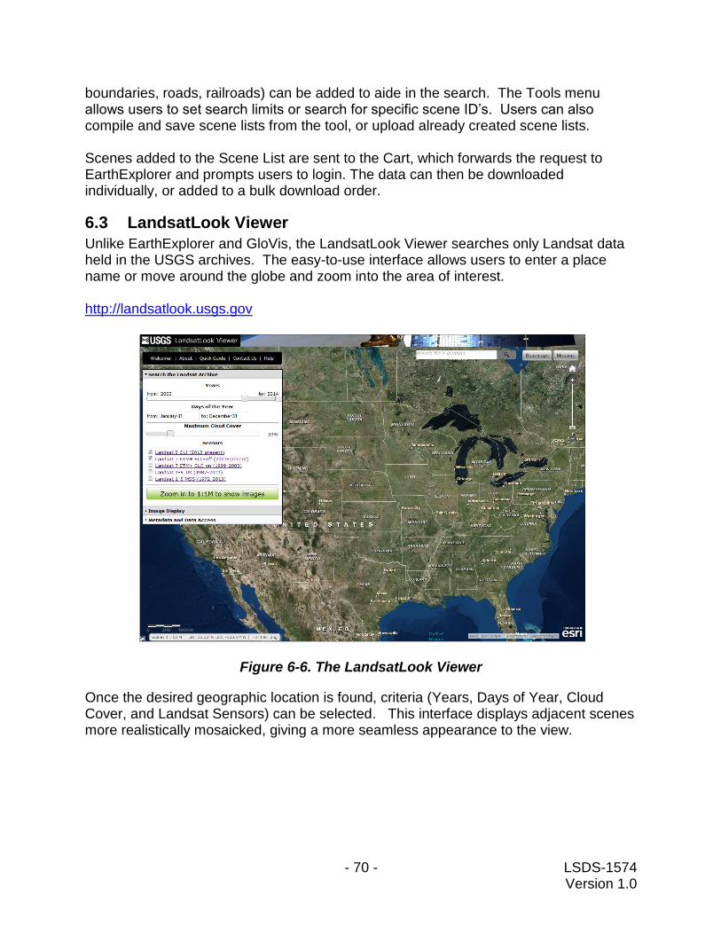
- 70 - LSDS-1574 Version 1.0

boundaries, roads, railroads) can be added to aide in the search. The Tools menu allows users to set search limits or search for specific scene ID’s. Users can also compile and save scene lists from the tool, or upload already created scene lists. Scenes added to the Scene List are sent to the Cart, which forwards the request to EarthExplorer and prompts users to login. The data can then be downloaded individually, or added to a bulk download order.

6.3 LandsatLook Viewer

Unlike EarthExplorer and GloVis, the LandsatLook Viewer searches only Landsat data held in the USGS archives. The easy-to-use interface allows users to enter a place name or move around the globe and zoom into the area of interest. http://landsatlook.usgs.gov

Figure 6-6. The LandsatLook Viewer

Once the desired geographic location is found, criteria (Years, Days of Year, Cloud Cover, and Landsat Sensors) can be selected. This interface displays adjacent scenes more realistically mosaicked, giving a more seamless appearance to the view.

http://landsatlook.usgs.gov/

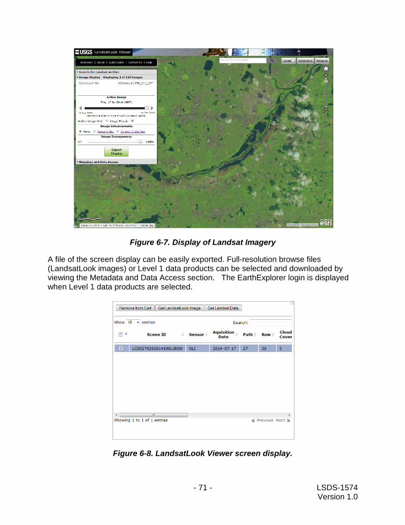
- 71 - LSDS-1574 Version 1.0

Figure 6-7. Display of Landsat Imagery

A file of the screen display can be easily exported. Full-resolution browse files (LandsatLook images) or Level 1 data products can be selected and downloaded by viewing the Metadata and Data Access section. The EarthExplorer login is displayed when Level 1 data products are selected.

Figure 6-8. LandsatLook Viewer screen display.

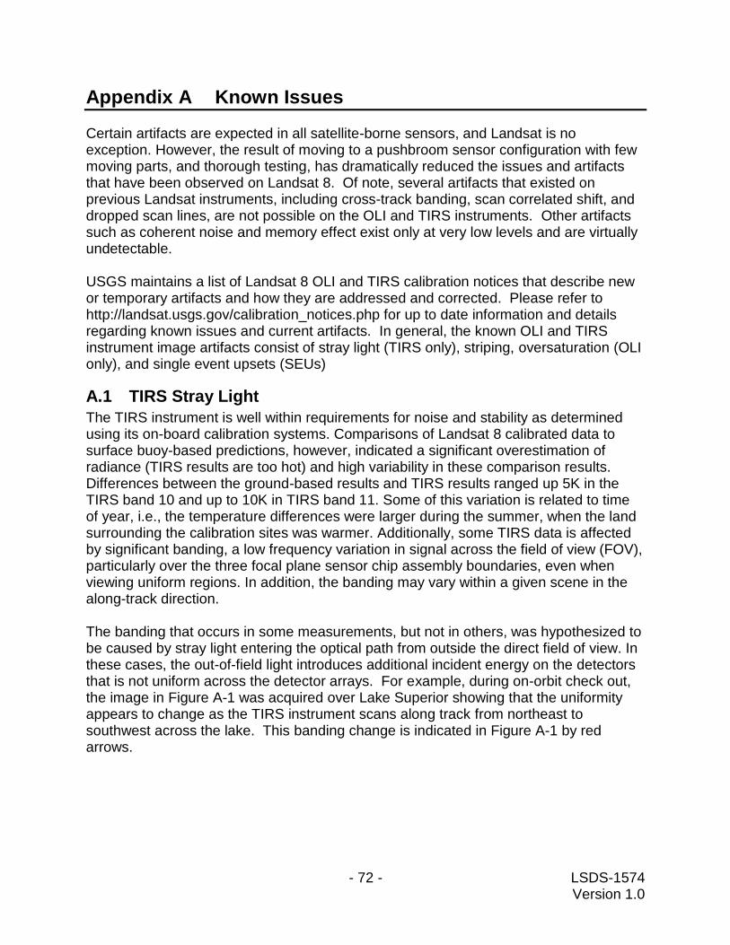
- 72 - LSDS-1574 Version 1.0

Appendix A Known Issues

Certain artifacts are expected in all satellite-borne sensors, and Landsat is no exception. However, the result of moving to a pushbroom sensor configuration with few moving parts, and thorough testing, has dramatically reduced the issues and artifacts that have been observed on Landsat 8. Of note, several artifacts that existed on previous Landsat instruments, including cross-track banding, scan correlated shift, and dropped scan lines, are not possible on the OLI and TIRS instruments. Other artifacts such as coherent noise and memory effect exist only at very low levels and are virtually undetectable. USGS maintains a list of Landsat 8 OLI and TIRS calibration notices that describe new or temporary artifacts and how they are addressed and corrected. Please refer to http://landsat.usgs.gov/calibration_notices.php for up to date information and details regarding known issues and current artifacts. In general, the known OLI and TIRS instrument image artifacts consist of stray light (TIRS only), striping, oversaturation (OLI only), and single event upsets (SEUs)

A.1 TIRS Stray Light

The TIRS instrument is well within requirements for noise and stability as determined using its on-board calibration systems. Comparisons of Landsat 8 calibrated data to surface buoy-based predictions, however, indicated a significant overestimation of radiance (TIRS results are too hot) and high variability in these comparison results. Differences between the ground-based results and TIRS results ranged up 5K in the TIRS band 10 and up to 10K in TIRS band 11. Some of this variation is related to time of year, i.e., the temperature differences were larger during the summer, when the land surrounding the calibration sites was warmer. Additionally, some TIRS data is affected by significant banding, a low frequency variation in signal across the field of view (FOV), particularly over the three focal plane sensor chip assembly boundaries, even when viewing uniform regions. In addition, the banding may vary within a given scene in the along-track direction. The banding that occurs in some measurements, but not in others, was hypothesized to be caused by stray light entering the optical path from outside the direct field of view. In these cases, the out-of-field light introduces additional incident energy on the detectors that is not uniform across the detector arrays. For example, during on-orbit check out, the image in Figure A-1 was acquired over Lake Superior showing that the uniformity appears to change as the TIRS instrument scans along track from northeast to southwest across the lake. This banding change is indicated in Figure A-1 by red arrows.

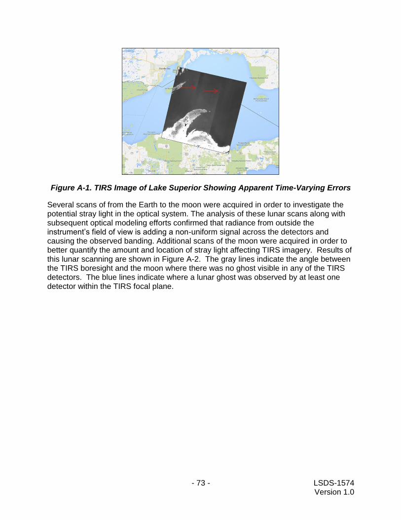
- 73 - LSDS-1574 Version 1.0

Figure A-1. TIRS Image of Lake Superior Showing Apparent Time-Varying Errors

Several scans of from the Earth to the moon were acquired in order to investigate the potential stray light in the optical system. The analysis of these lunar scans along with subsequent optical modeling efforts confirmed that radiance from outside the instrument’s field of view is adding a non-uniform signal across the detectors and causing the observed banding. Additional scans of the moon were acquired in order to better quantify the amount and location of stray light affecting TIRS imagery. Results of this lunar scanning are shown in Figure A-2. The gray lines indicate the angle between the TIRS boresight and the moon where there was no ghost visible in any of the TIRS detectors. The blue lines indicate where a lunar ghost was observed by at least one detector within the TIRS focal plane.

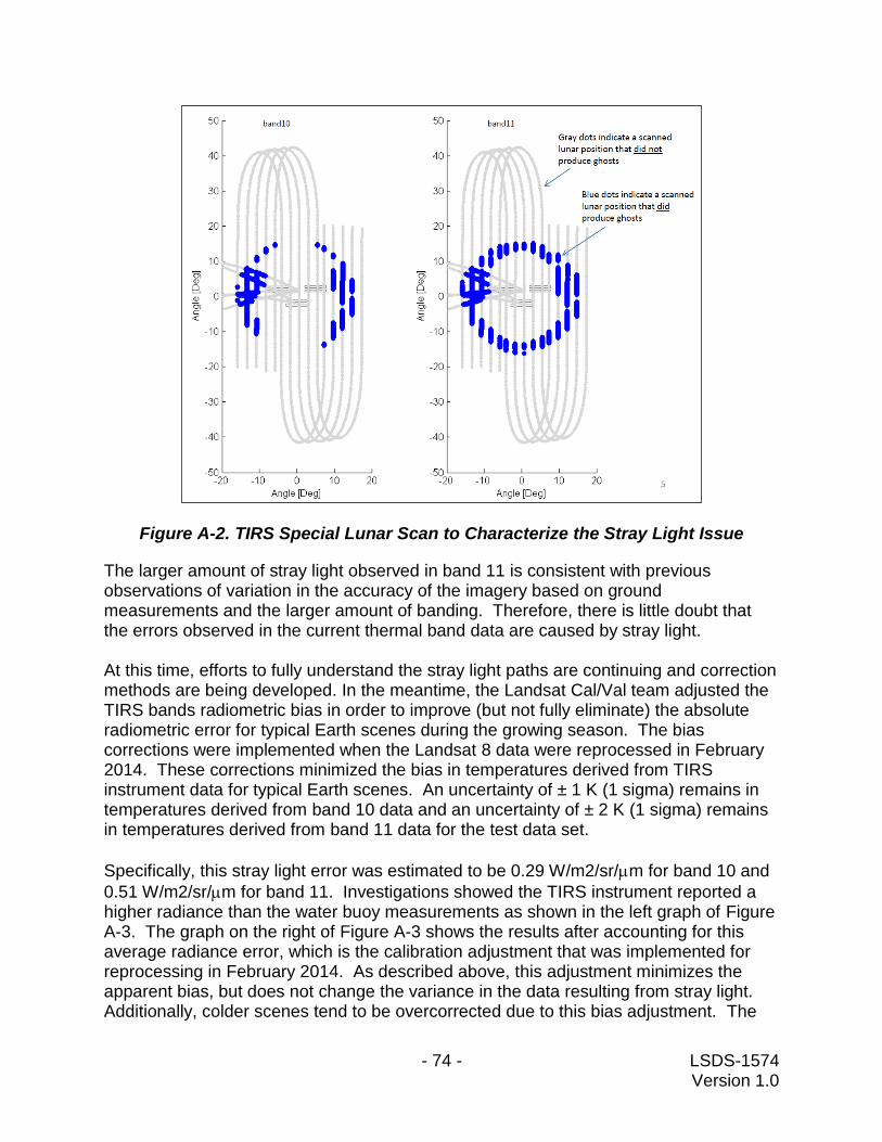
- 74 - LSDS-1574 Version 1.0

Figure A-2. TIRS Special Lunar Scan to Characterize the Stray Light Issue

The larger amount of stray light observed in band 11 is consistent with previous observations of variation in the accuracy of the imagery based on ground measurements and the larger amount of banding. Therefore, there is little doubt that the errors observed in the current thermal band data are caused by stray light. At this time, efforts to fully understand the stray light paths are continuing and correction methods are being developed. In the meantime, the Landsat Cal/Val team adjusted the TIRS bands radiometric bias in order to improve (but not fully eliminate) the absolute radiometric error for typical Earth scenes during the growing season. The bias corrections were implemented when the Landsat 8 data were reprocessed in February 2014. These corrections minimized the bias in temperatures derived from TIRS instrument data for typical Earth scenes. An uncertainty of ± 1 K (1 sigma) remains in temperatures derived from band 10 data and an uncertainty of ± 2 K (1 sigma) remains in temperatures derived from band 11 data for the test data set.

Specifically, this stray light error was estimated to be 0.29 W/m2/sr/m for band 10 and

0.51 W/m2/sr/m for band 11. Investigations showed the TIRS instrument reported a higher radiance than the water buoy measurements as shown in the left graph of Figure A-3. The graph on the right of Figure A-3 shows the results after accounting for this average radiance error, which is the calibration adjustment that was implemented for reprocessing in February 2014. As described above, this adjustment minimizes the apparent bias, but does not change the variance in the data resulting from stray light. Additionally, colder scenes tend to be overcorrected due to this bias adjustment. The

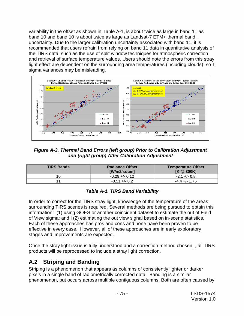
- 75 - LSDS-1574 Version 1.0

variability in the offset as shown in Table A-1, is about twice as large in band 11 as band 10 and band 10 is about twice as large as Landsat-7 ETM+ thermal band uncertainty. Due to the larger calibration uncertainty associated with band 11, it is recommended that users refrain from relying on band 11 data in quantitative analysis of the TIRS data, such as the use of split window techniques for atmospheric correction and retrieval of surface temperature values. Users should note the errors from this stray light effect are dependent on the surrounding area temperatures (including clouds), so 1 sigma variances may be misleading.

TIRS Bands Radiance Offset [W/m2/sr/um]

Temperature Offset [K @ 300K]

10 -0.29 +/- 0.12 -2.1 +/- 0.8

11 -0.51 +/- 0.2 -4.4 +/- 1.75

Table A-1. TIRS Band Variability

In order to correct for the TIRS stray light, knowledge of the temperature of the areas surrounding TIRS scenes is required. Several methods are being pursued to obtain this information: (1) using GOES or another coincident dataset to estimate the out of Field of View sigma; and l (2) estimating the out view signal based on in-scene statistics. Each of these approaches has pros and cons and none have been proven to be effective in every case. However, all of these approaches are in early exploratory stages and improvements are expected. Once the stray light issue is fully understood and a correction method chosen, , all TIRS products will be reprocessed to include a stray light correction.

A.2 Striping and Banding

Striping is a phenomenon that appears as columns of consistently lighter or darker pixels in a single band of radiometrically corrected data. Banding is a similar phenomenon, but occurs across multiple contiguous columns. Both are often caused by

Figure A-3. Thermal Band Errors (left group) Prior to Calibration Adjustment and (right group) After Calibration Adjustment

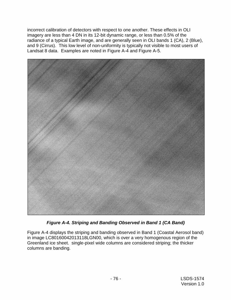
- 76 - LSDS-1574 Version 1.0

incorrect calibration of detectors with respect to one another. These effects in OLI imagery are less than 4 DN in its 12-bit dynamic range, or less than 0.5% of the radiance of a typical Earth image, and are generally seen in OLI bands 1 (CA), 2 (Blue), and 9 (Cirrus). This low level of non-uniformity is typically not visible to most users of Landsat 8 data. Examples are noted in Figure A-4 and Figure A-5.

Figure A-4. Striping and Banding Observed in Band 1 (CA Band)

Figure A-4 displays the striping and banding observed in Band 1 (Coastal Aerosol band) in image LC80160042013118LGN00, which is over a very homogenous region of the Greenland ice sheet. single-pixel wide columns are considered striping; the thicker columns are banding.

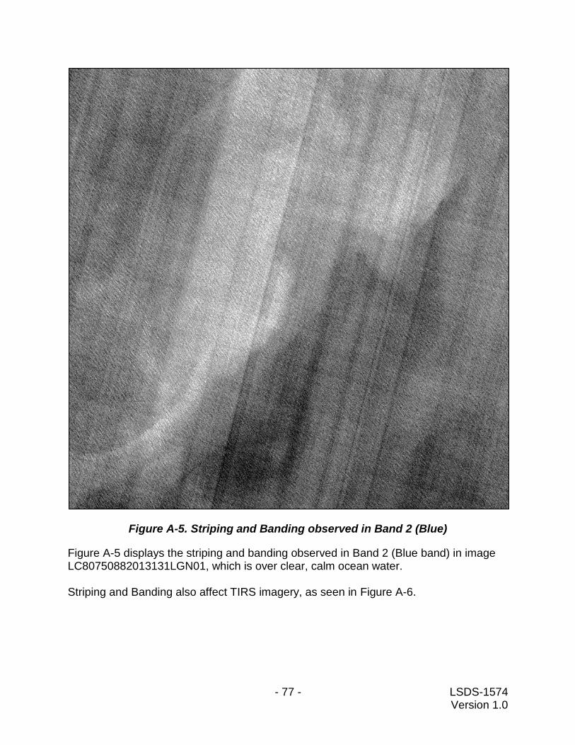
- 77 - LSDS-1574 Version 1.0

Figure A-5. Striping and Banding observed in Band 2 (Blue)

Figure A-5 displays the striping and banding observed in Band 2 (Blue band) in image LC80750882013131LGN01, which is over clear, calm ocean water. Striping and Banding also affect TIRS imagery, as seen in Figure A-6.

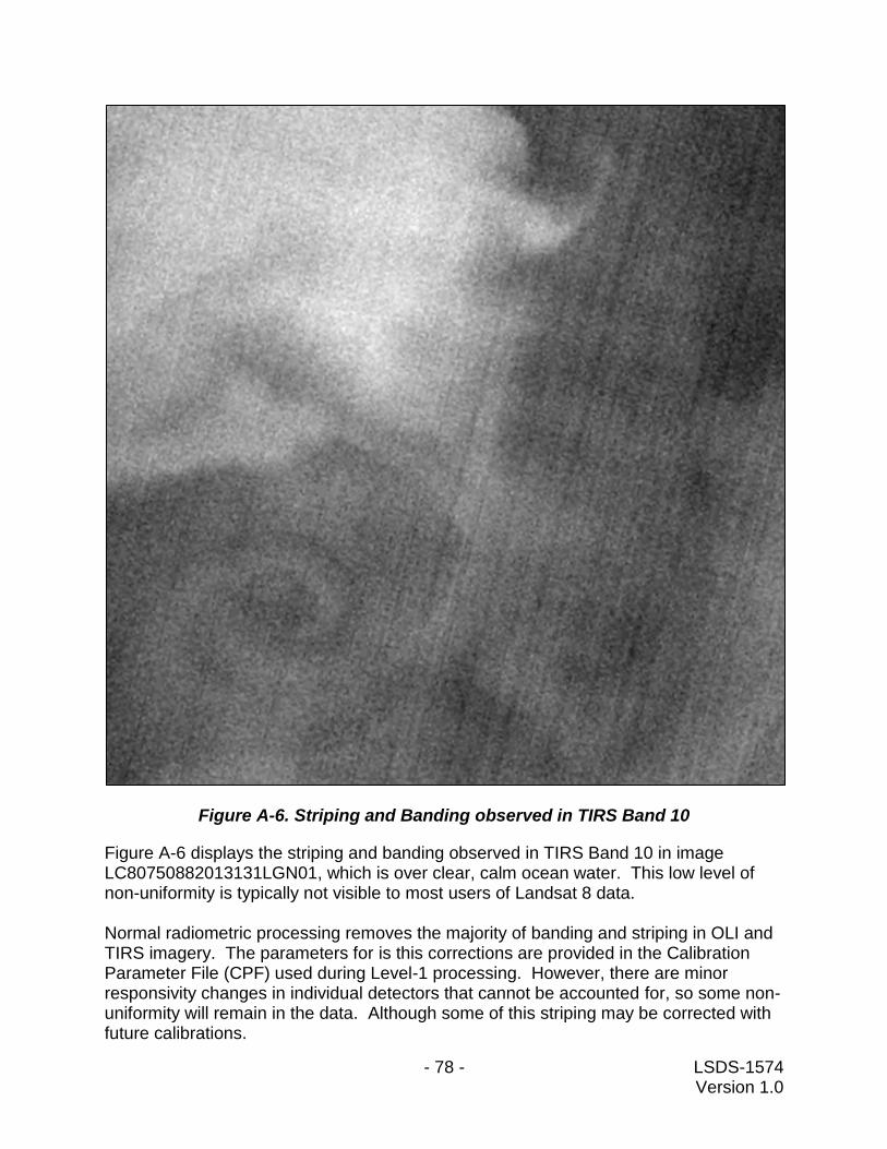
- 78 - LSDS-1574 Version 1.0

Figure A-6. Striping and Banding observed in TIRS Band 10

Figure A-6 displays the striping and banding observed in TIRS Band 10 in image LC80750882013131LGN01, which is over clear, calm ocean water. This low level of non-uniformity is typically not visible to most users of Landsat 8 data. Normal radiometric processing removes the majority of banding and striping in OLI and TIRS imagery. The parameters for is this corrections are provided in the Calibration Parameter File (CPF) used during Level-1 processing. However, there are minor responsivity changes in individual detectors that cannot be accounted for, so some non-uniformity will remain in the data. Although some of this striping may be corrected with future calibrations.

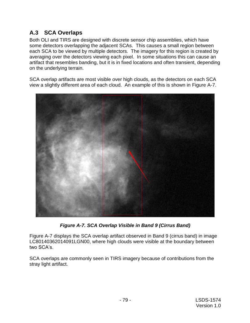
- 79 - LSDS-1574 Version 1.0

A.3 SCA Overlaps

Both OLI and TIRS are designed with discrete sensor chip assemblies, which have some detectors overlapping the adjacent SCAs. This causes a small region between each SCA to be viewed by multiple detectors. The imagery for this region is created by averaging over the detectors viewing each pixel. In some situations this can cause an artifact that resembles banding, but it is in fixed locations and often transient, depending on the underlying terrain. SCA overlap artifacts are most visible over high clouds, as the detectors on each SCA view a slightly different area of each cloud. An example of this is shown in Figure A-7.

Figure A-7. SCA Overlap Visible in Band 9 (Cirrus Band)

Figure A-7 displays the SCA overlap artifact observed in Band 9 (cirrus band) in image LC80140362014091LGN00, where high clouds were visible at the boundary between two SCA’s. SCA overlaps are commonly seen in TIRS imagery because of contributions from the stray light artifact.

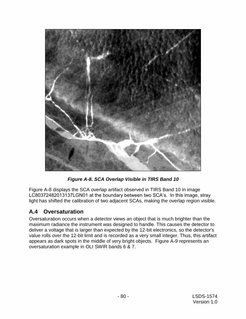
- 80 - LSDS-1574 Version 1.0

Figure A-8. SCA Overlap Visible in TIRS Band 10

Figure A-8 displays the SCA overlap artifact observed in TIRS Band 10 in image LC80372482013137LGN01 at the boundary between two SCA’s. In this image, stray light has shifted the calibration of two adjacent SCAs, making the overlap region visible.

A.4 Oversaturation

Oversaturation occurs when a detector views an object that is much brighter than the maximum radiance the instrument was designed to handle. This causes the detector to deliver a voltage that is larger than expected by the 12-bit electronics, so the detector's value rolls over the 12-bit limit and is recorded as a very small integer. Thus, this artifact appears as dark spots in the middle of very bright objects. Figure A-9 represents an oversaturation example in OLI SWIR bands 6 & 7.

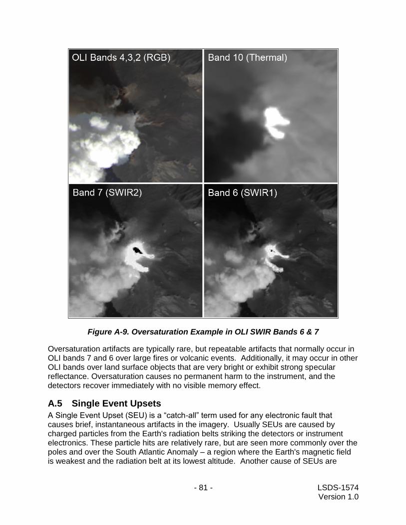
- 81 - LSDS-1574 Version 1.0

Figure A-9. Oversaturation Example in OLI SWIR Bands 6 & 7

Oversaturation artifacts are typically rare, but repeatable artifacts that normally occur in OLI bands 7 and 6 over large fires or volcanic events. Additionally, it may occur in other OLI bands over land surface objects that are very bright or exhibit strong specular reflectance. Oversaturation causes no permanent harm to the instrument, and the detectors recover immediately with no visible memory effect.

A.5 Single Event Upsets

A Single Event Upset (SEU) is a “catch-all” term used for any electronic fault that causes brief, instantaneous artifacts in the imagery. Usually SEUs are caused by charged particles from the Earth's radiation belts striking the detectors or instrument electronics. These particle hits are relatively rare, but are seen more commonly over the poles and over the South Atlantic Anomaly – a region where the Earth's magnetic field is weakest and the radiation belt at its lowest altitude. Another cause of SEUs are

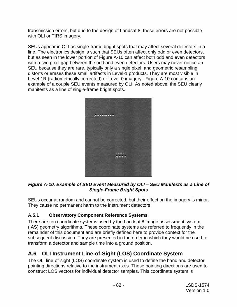
- 82 - LSDS-1574 Version 1.0

transmission errors, but due to the design of Landsat 8, these errors are not possible with OLI or TIRS imagery. SEUs appear in OLI as single-frame bright spots that may affect several detectors in a line. The electronics design is such that SEUs often affect only odd or even detectors, but as seen in the lower portion of Figure A-10 can affect both odd and even detectors with a two pixel gap between the odd and even detectors. Users may never notice an SEU because they are rare, typically only a single pixel, and geometric resampling distorts or erases these small artifacts in Level-1 products. They are most visible in Level-1R (radiometrically corrected) or Level-0 imagery. Figure A-10 contains an example of a couple SEU events measured by OLI. As noted above, the SEU clearly manifests as a line of single-frame bright spots.

Figure A-10. Example of SEU Event Measured by OLI – SEU Manifests as a Line of Single-Frame Bright Spots

SEUs occur at random and cannot be corrected, but their effect on the imagery is minor. They cause no permanent harm to the instrument detectors

A.5.1 Observatory Component Reference Systems

There are ten coordinate systems used by the Landsat 8 image assessment system (IAS) geometry algorithms. These coordinate systems are referred to frequently in the remainder of this document and are briefly defined here to provide context for the subsequent discussion. They are presented in the order in which they would be used to transform a detector and sample time into a ground position.

A.6 OLI Instrument Line-of-Sight (LOS) Coordinate System

The OLI line-of-sight (LOS) coordinate system is used to define the band and detector pointing directions relative to the instrument axes. These pointing directions are used to construct LOS vectors for individual detector samples. This coordinate system is

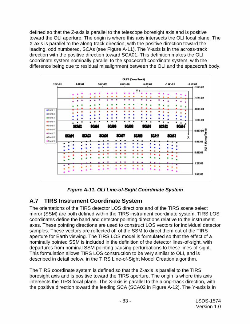
- 83 - LSDS-1574 Version 1.0

defined so that the Z-axis is parallel to the telescope boresight axis and is positive toward the OLI aperture. The origin is where this axis intersects the OLI focal plane. The X-axis is parallel to the along-track direction, with the positive direction toward the leading, odd numbered, SCAs (see Figure A-11). The Y-axis is in the across-track direction with the positive direction toward SCA01. This definition makes the OLI coordinate system nominally parallel to the spacecraft coordinate system, with the difference being due to residual misalignment between the OLI and the spacecraft body.

Figure A-11. OLI Line-of-Sight Coordinate System

A.7 TIRS Instrument Coordinate System

The orientations of the TIRS detector LOS directions and of the TIRS scene select mirror (SSM) are both defined within the TIRS instrument coordinate system. TIRS LOS coordinates define the band and detector pointing directions relative to the instrument axes. These pointing directions are used to construct LOS vectors for individual detector samples. These vectors are reflected off of the SSM to direct them out of the TIRS aperture for Earth viewing. The TIRS LOS model is formulated so that the effect of a nominally pointed SSM is included in the definition of the detector lines-of-sight, with departures from nominal SSM pointing causing perturbations to these lines-of-sight. This formulation allows TIRS LOS construction to be very similar to OLI, and is described in detail below, in the TIRS Line-of-Sight Model Creation algorithm. The TIRS coordinate system is defined so that the Z-axis is parallel to the TIRS boresight axis and is positive toward the TIRS aperture. The origin is where this axis intersects the TIRS focal plane. The X-axis is parallel to the along-track direction, with the positive direction toward the leading SCA (SCA02 in Figure A-12). The Y-axis is in

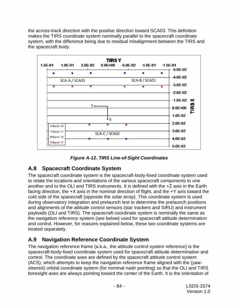
- 84 - LSDS-1574 Version 1.0

the across-track direction with the positive direction toward SCA03. This definition makes the TIRS coordinate system nominally parallel to the spacecraft coordinate system, with the difference being due to residual misalignment between the TIRS and the spacecraft body.

Figure A-12. TIRS Line-of-Sight Coordinates

A.8 Spacecraft Coordinate System

The spacecraft coordinate system is the spacecraft-body-fixed coordinate system used to relate the locations and orientations of the various spacecraft components to one another and to the OLI and TIRS instruments. It is defined with the +Z axis in the Earth facing direction, the +X axis in the nominal direction of flight, and the +Y axis toward the cold side of the spacecraft (opposite the solar array). This coordinate system is used during observatory integration and prelaunch test to determine the prelaunch positions and alignments of the attitude control sensors (star trackers and SIRU) and instrument payloads (OLI and TIRS). The spacecraft coordinate system is nominally the same as the navigation reference system (see below) used for spacecraft attitude determination and control. However, for reasons explained below, these two coordinate systems are treated separately.

A.9 Navigation Reference Coordinate System

The navigation reference frame (a.k.a., the attitude control system reference) is the spacecraft-body-fixed coordinate system used for spacecraft attitude determination and control. The coordinate axes are defined by the spacecraft attitude control system (ACS), which attempts to keep the navigation reference frame aligned with the (yaw-steered) orbital coordinate system (for nominal nadir pointing) so that the OLI and TIRS boresight axes are always pointing toward the center of the Earth. It is the orientation of

- 85 - LSDS-1574 Version 1.0

this coordinate system relative to the inertial coordinate system that is captured in spacecraft attitude data. Ideally, the navigation reference frame is the same as the spacecraft coordinate system. In practice, the navigation frame is based on the orientation of the absolute attitude sensor (i.e., star tracker) being used for attitude determination. Any errors in the orientation knowledge for this tracker with respect to the spacecraft body frame will lead to differences between the spacecraft and navigation coordinate systems. This becomes important if the absolute attitude sensor is changed, for example by switching from the primary to the redundant star tracker during on-orbit operations. Such an event would effectively redefine the navigation frame to be based on the redundant tracker with the difference between the spacecraft and navigation frames now resulting from redundant tracker alignment knowledge errors, rather than from primary tracker alignment knowledge errors. This redefinition would require updates to the on-orbit instrument-to-ACS alignment calibrations. Therefore, the spacecraft and navigation reference coordinate systems are different because the spacecraft coordinate system is fixed but the navigation reference can change.

A.10 SIRU Coordinate System

The spacecraft orientation rate data provided by the spacecraft attitude control system’s inertial measurement unit are referenced to the Space Inertial Reference Unit (SIRU) coordinate system. The SIRU consists of four rotation-sensitive axes. This configuration provides redundancy to protect against the failure of any one axis. The four SIRU axis directions are determined relative to the SIRU coordinate system, the orientation of which is itself measured relative to the spacecraft coordinate system both prelaunch and on-orbit, as part of the ACS calibration procedure. This alignment transformation is used by the IAS to convert the SIRU data contained in the Landsat 8 spacecraft ancillary data to the navigation reference coordinate system for blending with the ACS quaternions.

A.11 Orbital Coordinate System

The orbital coordinate system is centered at the spacecraft, and its orientation is based on the spacecraft position in inertial space (see Figure A-13). The origin is the spacecraft’s center of mass, with the Z-axis pointing from the spacecraft’s center of mass to the Earth’s center of mass. The Y-axis is the normalized cross product of the Z-axis and the instantaneous (inertial) velocity vector and corresponds to the negative of the instantaneous angular momentum vector direction. The X-axis is the cross product of the Y and Z-axes. The orbital coordinate system is used to convert spacecraft attitude, expressed as Earth-Centered Inertial (ECI) quaternions, to roll-pitch-yaw Euler angles.

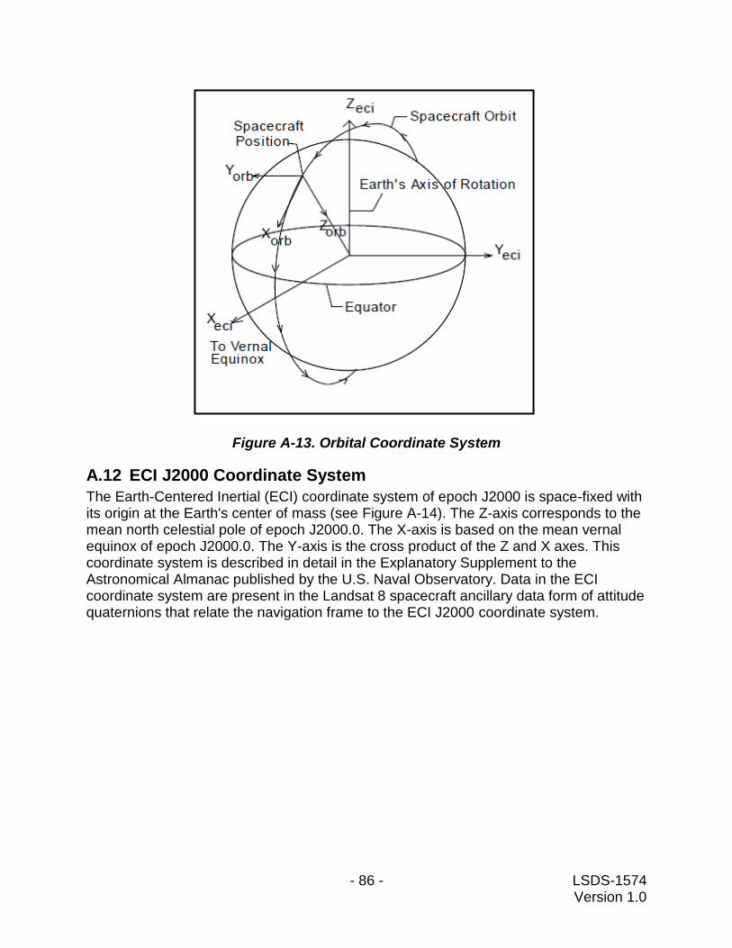
- 86 - LSDS-1574 Version 1.0

Figure A-13. Orbital Coordinate System

A.12 ECI J2000 Coordinate System

The Earth-Centered Inertial (ECI) coordinate system of epoch J2000 is space-fixed with its origin at the Earth's center of mass (see Figure A-14). The Z-axis corresponds to the mean north celestial pole of epoch J2000.0. The X-axis is based on the mean vernal equinox of epoch J2000.0. The Y-axis is the cross product of the Z and X axes. This coordinate system is described in detail in the Explanatory Supplement to the Astronomical Almanac published by the U.S. Naval Observatory. Data in the ECI coordinate system are present in the Landsat 8 spacecraft ancillary data form of attitude quaternions that relate the navigation frame to the ECI J2000 coordinate system.

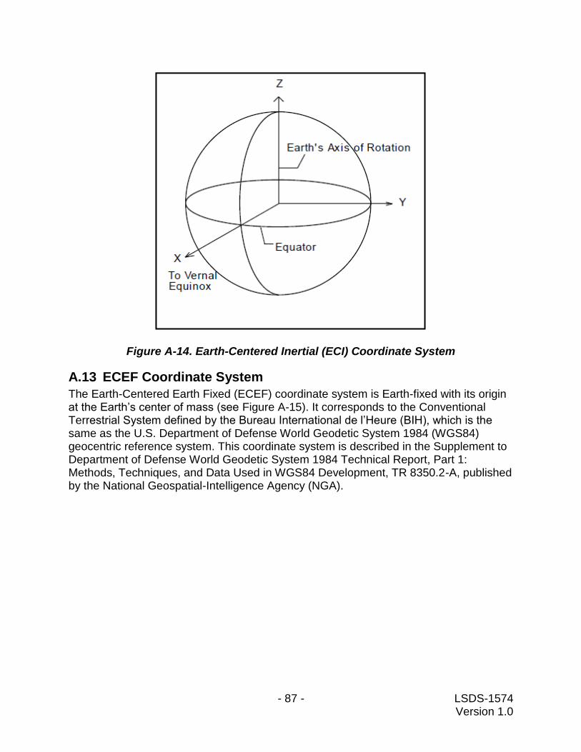
- 87 - LSDS-1574 Version 1.0

Figure A-14. Earth-Centered Inertial (ECI) Coordinate System

A.13 ECEF Coordinate System

The Earth-Centered Earth Fixed (ECEF) coordinate system is Earth-fixed with its origin at the Earth’s center of mass (see Figure A-15). It corresponds to the Conventional Terrestrial System defined by the Bureau International de l’Heure (BIH), which is the same as the U.S. Department of Defense World Geodetic System 1984 (WGS84) geocentric reference system. This coordinate system is described in the Supplement to Department of Defense World Geodetic System 1984 Technical Report, Part 1: Methods, Techniques, and Data Used in WGS84 Development, TR 8350.2-A, published by the National Geospatial-Intelligence Agency (NGA).

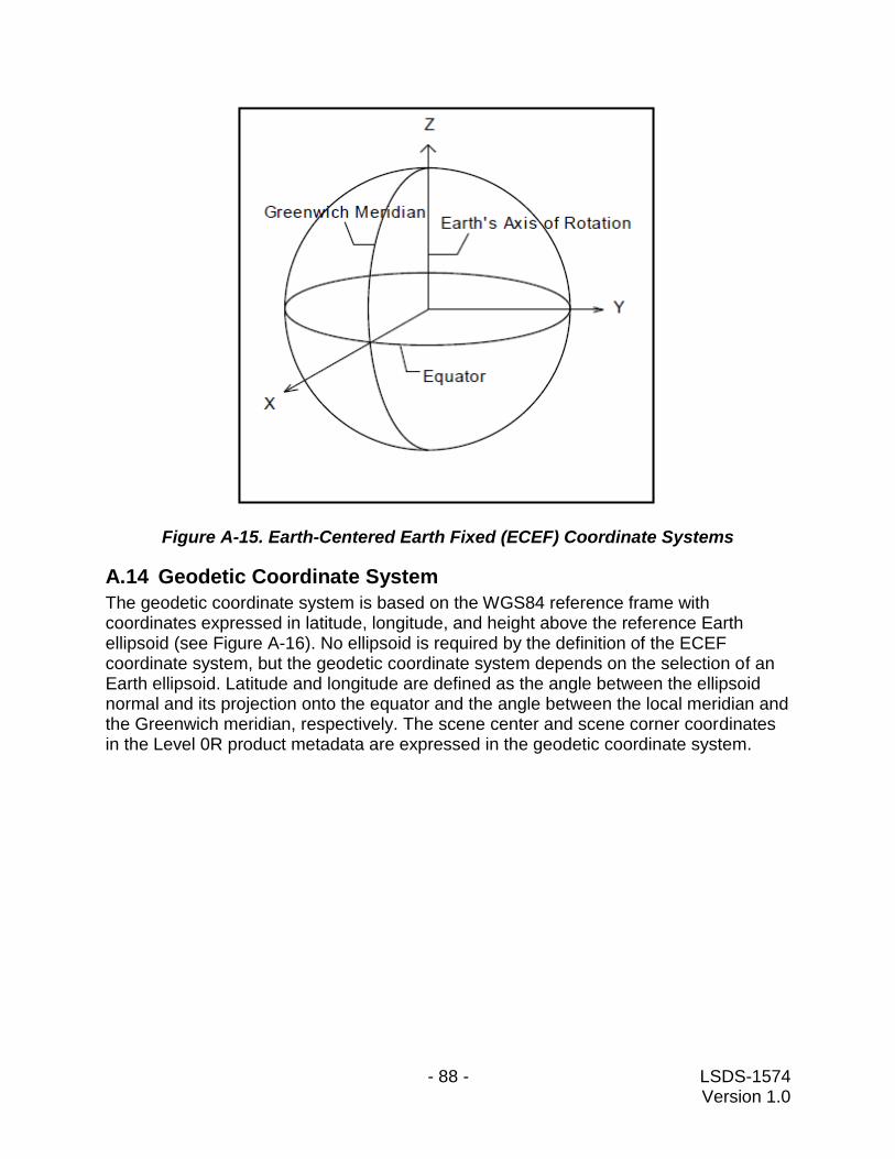
- 88 - LSDS-1574 Version 1.0

Figure A-15. Earth-Centered Earth Fixed (ECEF) Coordinate Systems

A.14 Geodetic Coordinate System

The geodetic coordinate system is based on the WGS84 reference frame with coordinates expressed in latitude, longitude, and height above the reference Earth ellipsoid (see Figure A-16). No ellipsoid is required by the definition of the ECEF coordinate system, but the geodetic coordinate system depends on the selection of an Earth ellipsoid. Latitude and longitude are defined as the angle between the ellipsoid normal and its projection onto the equator and the angle between the local meridian and the Greenwich meridian, respectively. The scene center and scene corner coordinates in the Level 0R product metadata are expressed in the geodetic coordinate system.

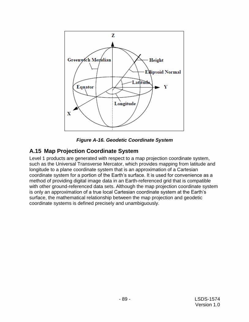
- 89 - LSDS-1574 Version 1.0

Figure A-16. Geodetic Coordinate System

A.15 Map Projection Coordinate System

Level 1 products are generated with respect to a map projection coordinate system, such as the Universal Transverse Mercator, which provides mapping from latitude and longitude to a plane coordinate system that is an approximation of a Cartesian coordinate system for a portion of the Earth’s surface. It is used for convenience as a method of providing digital image data in an Earth-referenced grid that is compatible with other ground-referenced data sets. Although the map projection coordinate system is only an approximation of a true local Cartesian coordinate system at the Earth’s surface, the mathematical relationship between the map projection and geodetic coordinate systems is defined precisely and unambiguously.

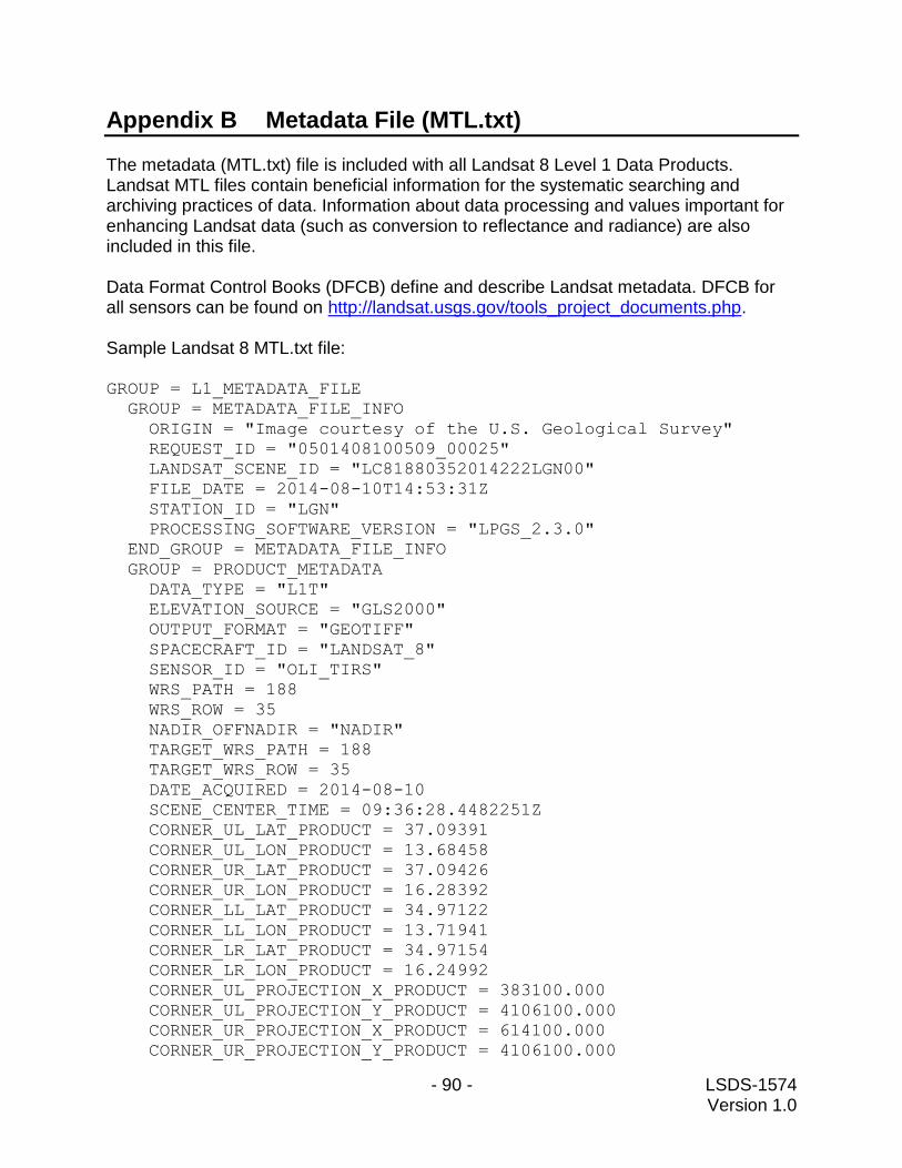
- 90 - LSDS-1574 Version 1.0

Appendix B Metadata File (MTL.txt)

The metadata (MTL.txt) file is included with all Landsat 8 Level 1 Data Products. Landsat MTL files contain beneficial information for the systematic searching and archiving practices of data. Information about data processing and values important for enhancing Landsat data (such as conversion to reflectance and radiance) are also included in this file. Data Format Control Books (DFCB) define and describe Landsat metadata. DFCB for all sensors can be found on http://landsat.usgs.gov/tools_project_documents.php. Sample Landsat 8 MTL.txt file: GROUP = L1_METADATA_FILE

GROUP = METADATA_FILE_INFO

ORIGIN = "Image courtesy of the U.S. Geological Survey"

REQUEST_ID = "0501408100509_00025"

LANDSAT_SCENE_ID = "LC81880352014222LGN00"

FILE_DATE = 2014-08-10T14:53:31Z

STATION_ID = "LGN"

PROCESSING_SOFTWARE_VERSION = "LPGS_2.3.0"

END_GROUP = METADATA_FILE_INFO

GROUP = PRODUCT_METADATA

DATA_TYPE = "L1T"

ELEVATION_SOURCE = "GLS2000"

OUTPUT_FORMAT = "GEOTIFF"

SPACECRAFT_ID = "LANDSAT_8"

SENSOR_ID = "OLI_TIRS"

WRS_PATH = 188

WRS_ROW = 35

NADIR_OFFNADIR = "NADIR"

TARGET_WRS_PATH = 188

TARGET_WRS_ROW = 35

DATE_ACQUIRED = 2014-08-10

SCENE_CENTER_TIME = 09:36:28.4482251Z

CORNER_UL_LAT_PRODUCT = 37.09391

CORNER_UL_LON_PRODUCT = 13.68458

CORNER_UR_LAT_PRODUCT = 37.09426

CORNER_UR_LON_PRODUCT = 16.28392

CORNER_LL_LAT_PRODUCT = 34.97122

CORNER_LL_LON_PRODUCT = 13.71941

CORNER_LR_LAT_PRODUCT = 34.97154

CORNER_LR_LON_PRODUCT = 16.24992

CORNER_UL_PROJECTION_X_PRODUCT = 383100.000

CORNER_UL_PROJECTION_Y_PRODUCT = 4106100.000

CORNER_UR_PROJECTION_X_PRODUCT = 614100.000

CORNER_UR_PROJECTION_Y_PRODUCT = 4106100.000

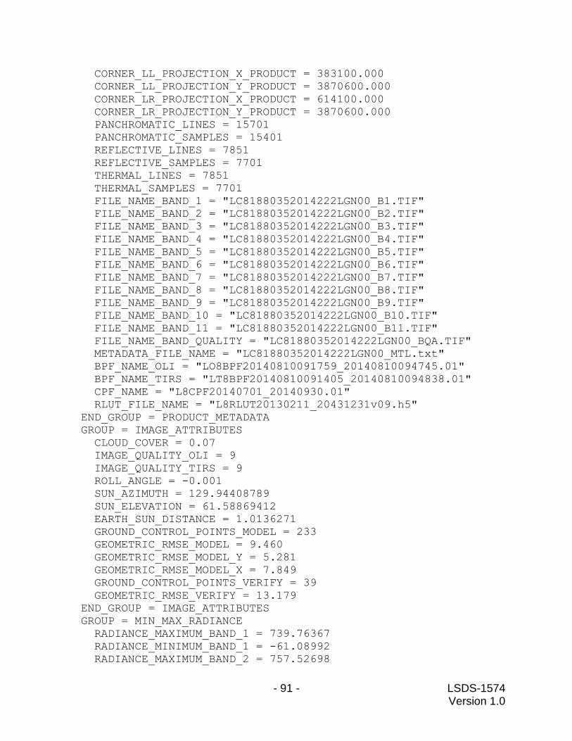
http://landsat.usgs.gov/tools_project_documents.php

- 91 - LSDS-1574 Version 1.0

CORNER_LL_PROJECTION_X_PRODUCT = 383100.000

CORNER_LL_PROJECTION_Y_PRODUCT = 3870600.000

CORNER_LR_PROJECTION_X_PRODUCT = 614100.000

CORNER_LR_PROJECTION_Y_PRODUCT = 3870600.000

PANCHROMATIC_LINES = 15701

PANCHROMATIC_SAMPLES = 15401

REFLECTIVE_LINES = 7851

REFLECTIVE_SAMPLES = 7701

THERMAL_LINES = 7851

THERMAL_SAMPLES = 7701

FILE_NAME_BAND_1 = "LC81880352014222LGN00_B1.TIF"











FILE_NAME_BAND_QUALITY = "LC81880352014222LGN00_BQA.TIF"

METADATA_FILE_NAME = "LC81880352014222LGN00_MTL.txt"

BPF_NAME_OLI = "LO8BPF20140810091759_20140810094745.01"

BPF_NAME_TIRS = "LT8BPF20140810091405_20140810094838.01"

CPF_NAME = "L8CPF20140701_20140930.01"

RLUT_FILE_NAME = "L8RLUT20130211_20431231v09.h5"

END_GROUP = PRODUCT_METADATA

GROUP = IMAGE_ATTRIBUTES

CLOUD_COVER = 0.07

IMAGE_QUALITY_OLI = 9

IMAGE_QUALITY_TIRS = 9

ROLL_ANGLE = -0.001

SUN_AZIMUTH = 129.94408789

SUN_ELEVATION = 61.58869412

EARTH_SUN_DISTANCE = 1.0136271

GROUND_CONTROL_POINTS_MODEL = 233

GEOMETRIC_RMSE_MODEL = 9.460

GEOMETRIC_RMSE_MODEL_Y = 5.281

GEOMETRIC_RMSE_MODEL_X = 7.849

GROUND_CONTROL_POINTS_VERIFY = 39

GEOMETRIC_RMSE_VERIFY = 13.179

END_GROUP = IMAGE_ATTRIBUTES

GROUP = MIN_MAX_RADIANCE

RADIANCE_MAXIMUM_BAND_1 = 739.76367

RADIANCE_MINIMUM_BAND_1 = -61.08992


- 92 - LSDS-1574 Version 1.0

















RADIANCE_MINIMUM_BAND_10 = 0.10033


RADIANCE_MINIMUM_BAND_11 = 0.10033

END_GROUP = MIN_MAX_RADIANCE

GROUP = MIN_MAX_REFLECTANCE

REFLECTANCE_MAXIMUM_BAND_1 = 1.210700

REFLECTANCE_MINIMUM_BAND_1 = -0.099980

















END_GROUP = MIN_MAX_REFLECTANCE

GROUP = MIN_MAX_PIXEL_VALUE

QUANTIZE_CAL_MAX_BAND_1 = 65535

QUANTIZE_CAL_MIN_BAND_1 = 1





- 93 - LSDS-1574 Version 1.0

















END_GROUP = MIN_MAX_PIXEL_VALUE

GROUP = RADIOMETRIC_RESCALING

RADIANCE_MULT_BAND_1 = 1.2220E-02











RADIANCE_ADD_BAND_1 = -61.10214









RADIANCE_ADD_BAND_10 = 0.10000

RADIANCE_ADD_BAND_11 = 0.10000

REFLECTANCE_MULT_BAND_1 = 2.0000E-05







- 94 - LSDS-1574 Version 1.0



REFLECTANCE_ADD_BAND_1 = -0.100000









END_GROUP = RADIOMETRIC_RESCALING

GROUP = TIRS_THERMAL_CONSTANTS

K1_CONSTANT_BAND_10 = 774.89




END_GROUP = TIRS_THERMAL_CONSTANTS

GROUP = PROJECTION_PARAMETERS

MAP_PROJECTION = "UTM"

DATUM = "WGS84"

ELLIPSOID = "WGS84"

UTM_ZONE = 33

GRID_CELL_SIZE_PANCHROMATIC = 15.00

GRID_CELL_SIZE_REFLECTIVE = 30.00

GRID_CELL_SIZE_THERMAL = 30.00

ORIENTATION = "NORTH_UP"

RESAMPLING_OPTION = "CUBIC_CONVOLUTION"

END_GROUP = PROJECTION_PARAMETERS

END_GROUP = L1_METADATA_FILE

END

- 95 - LSDS-1574 Version 1.0

References

Please see http://landsat.usgs.gov/tools_acronyms_ALL.php for a list of acronyms. Storey, James, Michael Choate, and Kenton Lee. "Landsat 8 Operational Land Imager On-Orbit Geometric Calibration and Performance." Remote Sensing 6, no. 11 (2014): 11127-11152. Storey, James, Michael Choate, and Donald Moe. "Landsat 8 thermal infrared sensor geometric characterization and calibration." Remote Sensing 6, no. 11 (2014): 11153-11181. Markham, Brian, Julia Barsi, Geir Kvaran, Lawrence Ong, Edward Kaita, Stuart Biggar, Jeffrey Czapla-Myers, Nischal Mishra, and Dennis Helder. "Landsat-8 Operational Land Imager radiometric calibration and stability." Remote Sensing 6, no. 12 (2014): 12275-12308. Montanaro, Matthew, Raviv Levy, and Brian Markham. "On-orbit radiometric performance of the Landsat 8 Thermal Infrared Sensor." Remote Sensing 6, no. 12 (2014): 11753-11769. Barsi, Julia A., John R. Schott, Simon J. Hook, Nina G. Raqueno, Brian L. Markham, and Robert G. Radocinski. "Landsat-8 Thermal Infrared Sensor (TIRS) Vicarious Radiometric Calibration." Remote Sensing 6, no. 11 (2014): 11607-11626. Cook, Monica, John R. Schott, John Mandel, and Nina Raqueno. "Development of an Operational Calibration Methodology for the Landsat Thermal Data Archive and Initial Testing of the Atmospheric Compensation Component of a Land Surface Temperature (LST) Product from the Archive." Remote Sensing 6, no. 11 (2014): 11244-11266. Gerace, Aaron, John Schott, Michael Gartley, and Matthew Montanaro. "An Analysis of the Side Slither On-Orbit Calibration Technique Using the DIRSIG Model." Remote Sensing 6, no. 11 (2014): 10523-10545. Montanaro, Matthew, Aaron Gerace, Allen Lunsford, and Dennis Reuter. "Stray light artifacts in imagery from the Landsat 8 Thermal Infrared Sensor." Remote Sensing 6, no. 11 (2014): 10435-10456. Knight, Edward J., and Geir Kvaran. "Landsat-8 operational land imager design, characterization and performance." Remote Sensing 6, no. 11 (2014): 10286-10305. Barsi, Julia A., Kenton Lee, Geir Kvaran, Brian L. Markham, and Jeffrey A. Pedelty. "The spectral response of the Landsat-8 operational land imager." Remote Sensing 6, no. 10 (2014): 10232-10251.

http://landsat.usgs.gov/tools_acronyms_ALL.php

- 96 - LSDS-1574 Version 1.0

Montanaro, Matthew, Allen Lunsford, Zelalem Tesfaye, Brian Wenny, and Dennis Reuter. "Radiometric calibration methodology of the Landsat 8 Thermal Infrared Sensor." Remote Sensing 6, no. 9 (2014): 8803-8821. Morfitt, Ron, Julia Barsi, Raviv Levy, Brian Markham, Esad Micijevic, Lawrence Ong, Pat Scaramuzza, and Kelly Vanderwerff. "Landsat-8 Operational Land Imager (OLI) radiometric performance on-orbit." Remote Sensing 7, no. 2 (2015): 2208-2237. Mishra, Nischal, Md Obaidul Haque, Larry Leigh, David Aaron, Dennis Helder, and Brian Markham. "Radiometric Cross Calibration of Landsat 8 Operational Land Imager (OLI) and Landsat 7 Enhanced Thematic Mapper Plus (ETM+)." Remote Sensing 6, no. 12 (2014): 12619-12638. Wenny, Brian N., Dennis Helder, Jungseok Hong, Larry Leigh, Kurtis J. Thome, and Dennis Reuter. "Pre-and post-launch spatial quality of the Landsat 8 Thermal Infrared Sensor." Remote Sensing 7, no. 2 (2015): 1962-1980. Irons, James R., John L. Dwyer, and Julia A. Barsi. "The next Landsat satellite: The Landsat data continuity mission." Remote Sensing of Environment 122 (2012): 11-21. Irons, James R., and John L. Dwyer. "An overview of the Landsat Data Continuity Mission." In SPIE Defense, Security, and Sensing, pp. 769508-769508. International Society for Optics and Photonics, 2010. Arvidson, Terry, Samuel Goward, John Gasch, and Darrel Williams. "Landsat-7 Long-Term Acquisition Plan." Photogrammetric Engineering & Remote Sensing 72, no. 10 (2006): 1137-1146. Rice, Robert F., Pen-Shu Yeh, and Warner H. Miller. "Algorithms for high speed universal noiseless coding." In Proceedings of the AIAA Computing in Aerospace 9 Conference, pp. 19-21. 1993. EarthExplorer Tutorial. <https://lta.cr.usgs.gov/ee_help> EarthExplorer Registration. <https://earthexplorer.usgs.gov/register/> GloVis Quick Start Guide. <http://glovis.usgs.gov/QuickStart.shtml> LandsatLook Viewer User Documentation. <http://landsat.usgs.gov/LandsatLook_Viewer.php> Landsat Data Products. <http://landsat.usgs.gov> Landsat 8 Mission Data Format Control Book. <http://landsat.usgs.gov/documents/LDCM-DFCB-001.pdf>

https://lta.cr.usgs.gov/ee_help

https://earthexplorer.usgs.gov/register/

http://glovis.usgs.gov/QuickStart.shtml

http://landsat.usgs.gov/LandsatLook_Viewer.php

http://landsat.usgs.gov/


- 97 - LSDS-1574 Version 1.0

Landsat 8 Level 0 Reformatted Data Format Control Book. <http://landsat.usgs.gov/documents/LDCM-DFCB-002.pdf> Landsat 8 Level 1 Data Format Control Book. <http://landsat.usgs.gov/documents/Landsat8_Level1_Data_Format_Control_Book_LSDS-809.pdf> Landsat 8 Cal/Val Algorithm Description Document. <http://landsat.usgs.gov/documents/LDCM_CVT_ADD.pdf> Note: The above listed files are located at http://landsat.usgs.gov/tools_project_documents.php Landsat 8 Fact Sheet. <http://pubs.usgs.gov/fs/2013/3060/pdf/fs2013-3060.pdf> (linked from http://landsat.usgs.gov/about_project_descriptions.php)

Landsat 8 (L8) Operational Land Imager (OLI) and Thermal Infrared Sensor (TIRS) Calibration Notices. <http://landsat.usgs.gov/calibration_notices.php> Landsat 8 Overview. <http://landsat.usgs.gov/landsat8.php> LandsatLook Images. <http://landsat.usgs.gov/LandsatLookImages.php> USGS Landsat User Services Contact USGS Landsat User Services with any questions regarding these interfaces or Landsat data products, M-F 8:00 am to 4:00 p.m. CT: [email protected] 1-605-594-6151 1-800-252-4547


http://landsat.usgs.gov/documents/Landsat8_Level1_Data_Format_Control_Book_LSDS-809.pdf

http://landsat.usgs.gov/documents/Landsat8_Level1_Data_Format_Control_Book_LSDS-809.pdf

http://landsat.usgs.gov/documents/LDCM_CVT_ADD.pdf

http://landsat.usgs.gov/tools_project_documents.php

http://pubs.usgs.gov/fs/2013/3060/pdf/fs2013-3060.pdf

http://landsat.usgs.gov/about_project_descriptions.php

http://landsat.usgs.gov/calibration_notices.php

http://landsat.usgs.gov/landsat8.php

http://landsat.usgs.gov/LandsatLookImages.php

Documents

LANDSAT 8 (L8) DATA USERS HANDBOOK - WordPress.com · The Landsat 8 observatory offers these features: Data Continuity: Landsat 8 is the latest in a continuous series of land remote