Land Use Mix and Pedestrian Travel Behavior: Advancements

Portland State University Portland State University

PDXScholar PDXScholar

Dissertations and Theses Dissertations and Theses

Winter 3-7-2017

Land Use Mix and Pedestrian Travel Behavior: Land Use Mix and Pedestrian Travel Behavior:

Advancements in Conceptualization and Advancements in Conceptualization and

Measurement Measurement

Steven Robert Gehrke Portland State University

Follow this and additional works at: https://pdxscholar.library.pdx.edu/open_access_etds

Part of the Civil and Environmental Engineering Commons, and the Transportation Commons

Let us know how access to this document benefits you.

Recommended Citation Recommended Citation Gehrke, Steven Robert, "Land Use Mix and Pedestrian Travel Behavior: Advancements in Conceptualization and Measurement" (2017). Dissertations and Theses. Paper 3477. https://doi.org/10.15760/etd.5361

This Dissertation is brought to you for free and open access. It has been accepted for inclusion in Dissertations and Theses by an authorized administrator of PDXScholar. Please contact us if we can make this document more accessible: [email protected].

https://pdxscholar.library.pdx.edu/

https://pdxscholar.library.pdx.edu/open_access_etds

https://pdxscholar.library.pdx.edu/etds

https://pdxscholar.library.pdx.edu/open_access_etds?utm_source=pdxscholar.library.pdx.edu%2Fopen_access_etds%2F3477&utm_medium=PDF&utm_campaign=PDFCoverPages

http://network.bepress.com/hgg/discipline/251?utm_source=pdxscholar.library.pdx.edu%2Fopen_access_etds%2F3477&utm_medium=PDF&utm_campaign=PDFCoverPages

http://network.bepress.com/hgg/discipline/1068?utm_source=pdxscholar.library.pdx.edu%2Fopen_access_etds%2F3477&utm_medium=PDF&utm_campaign=PDFCoverPages

http://library.pdx.edu/services/pdxscholar-services/pdxscholar-feedback/

https://doi.org/10.15760/etd.5361

mailto:[email protected]

Land Use Mix and Pedestrian Travel Behavior:

Advancements in Conceptualization and Measurement

by

Steven Robert Gehrke

A dissertation submitted in partial fulfillment of the requirements for the degree of

Doctor of Philosophy in

Civil and Environmental Engineering

Dissertation Committee: Kelly J. Clifton, Chair

Christopher M. Monsere Liming Wang Jennifer Dill

Portland State University 2017

© 2017 Steven Robert Gehrke

i

Abstract

Smart growth policies have often emphasized the importance of land use mix as

an intervention beholding of lasting urban planning and public health benefits. Past

transportation-land use research has identified potential efficiency gains achieved by

mixed-use neighborhoods and the subsequent shortening of trip lengths; whereas,

public health research has accredited increased land use mixing as an effective policy for

facilitating greater physical activity. However, despite the celebrated transportation,

land use, and health benefits of improved land use mixing and the extent of topical

attention, no consensus has been reached regarding the conceptualization and

measurement of this key smart growth principle or the magnitude of its link to walking.

This dissertation, comprised of three empirical studies, explores this topic in detail.

In the first study, activity-based transportation and landscape ecology theory

contributed to the introduction of a multifaceted land use mix construct reflected by a

set of composition and configuration indicators. This activity-related land use mix

construct, and not the commonly used entropy index, was a significant built

environmental determinant of walk mode choice and home-based walk trip frequency.

In the second study, structural equation modeling was used to establish a connection

between residing in a smart growth neighborhood and home-based pedestrian travel.

This study discovered a multidimensional depiction of the traveler’s residential

environment that was reflective of local land use mix, employment concentration, and

pedestrian-oriented design. The second-order factor, which described a smart growth

ii

neighborhood, had a strong and positive effect on the household-level decision to walk

for transportation-related and discretionary travel when assessed in a multidirectional

conceptual framework.

In the final study, the influence of geographic scale selection on the connection

between the built environment and active and auto-related travel was explored.

Informed by this sensitivity analysis, which underlined the existence of scaling and

zoning effects, mode choice for both work and nonwork travel as a function of

individual, household, transportation, and built environment features at the home

location and destination was modeled. These discrete choice analysis results found that

measures of land use mix and density at each trip end had the strongest effect on the

decision to walk rather drive or ride in a vehicle for nonwork trips. In all, the findings

from this dissertation provide policymakers and practitioners greater specificity in the

measurement of land use mix and its connection to pedestrian travel behavior.

iii

Acknowledgments

Completion of this dissertation would not have been imaginable without the

lasting contributions, advice, and support of many colleagues, friends, and family

members. Receipt of a National Institute for Transportation and Communities (NITC)

Dissertation Fellowship and the Regional Science Association International’s Stan

Czamanski Prize provided the financial support to conduct this research. I was also

fortunate to begin my PhD program as data collection for the Oregon Household Activity

Survey by the Oregon Modeling Steering Committee was wrapping up. These travel data

and the land use information generously shared by Portland Metro, Mid-Willamette

Valley Council of Governments, and Lane Council of Governments were invaluable to this

dissertation research.

I am thankful for the guidance of my advisor, Kelly Clifton. During the past half-

decade, she has helped to shape my thinking on many transportation-land use issues,

delivered mentorship on applied research projects, exhibited patience as I advanced my

technical proficiencies, and presented me with the independence to pursue this

dissertation research agenda. Our discussions at conferences and coffee shops were

instrumental toward establishing the theoretical basis and research design for my

dissertation proposal and first two empirical studies. As an incoming doctoral student

with limited civil engineering training, Chris Monsere had the undesirable task of

introducing me to the R programming language. For this early instruction and his tacit

pressure to better situate my work within the profession of transportation engineering, I

iv

am very appreciative. I am also indebted to the teaching and direction of Liming Wang.

As a professor and dissertation committee member, he has continuously challenged me

to strengthen my analytic strategies, and provided useful and critical feedback on the

design of my third empirical study. Further, I would like to sincerely thank Jennifer Dill for

imparting her valued expertise on transportation planning to this dissertation. Her testing

of the theoretical underpinnings and practical implications of this work has, in my opinion,

helped to fashion a stronger and more important study.

The accomplishment of a finished dissertation is wrought with trials and

tribulations, which I could not have navigated without the camaraderie of my fellow

classmates and peers at PSU. I met Patrick Singleton at our new graduate student

orientation in spring 2011. We have since shared many inspiring conversations and

toasted many tasty microbrews. Since this time, he has always selflessly offered his

assistance in resolving a number of my more vexing methodologic challenges. I am further

grateful for the companionship of my fellow cubicle compatriots, Kristi Currans and Alex

Bigazzi, and other friends from our PhT collaborative, including Joe Broach, who were

always eager to exchange ideas and offer comical respite during this collective academic

experience.

I am eternally thankful for the heartfelt compassion and limitless support of my

wife, Olivia Lindly. She, time and again, listened to me proclaim the overwhelming

insecurity and high anxiety that I felt at various points on this journey, and always kept

me grounded by articulating her unwavering confidence that I would one day finish and

v

reminding me that I embarked on said journey under my own volition. Olivia is incredibly

thoughtful and the perfect confidant. I would also like to express my gratitude to my

parents, Debbie and Steve, and sister, Jackie, who have offered endless encouragement.

Finally, I am blessed by the unconditional love of my son, Eliot. He may never be

interested in this research, but his birth motivated me to defend my dissertation before

his first birthday. I did so with two days to spare.

vi

Table of Contents Abstract ................................................................................................................................. i Acknowledgments ............................................................................................................... iii List of Tables ..................................................................................................................... viii List of Figures ...................................................................................................................... ix Chapter 1: Introduction ...................................................................................................... 1

1.1 Context .................................................................................................................... 1 1.2 Motivation ............................................................................................................... 3 1.3 Objectives ................................................................................................................ 7 1.4 Overview ................................................................................................................. 8

Chapter 2: Toward a Spatial-Temporal Measure of Land Use Mix ................................... 11 2.1 Land Use Mix and Active Travel ............................................................................ 11

2.1.1 Land use mix and active travel by trip purpose ........................................... 13 2.1.2 Land use mix at the trip end and active travel ............................................ 17 2.1.3 Land use mix components ........................................................................... 19

2.2 Land Use Interaction ............................................................................................. 20 2.2.1 Measuring land use interaction ................................................................... 22 2.2.2 Concerns in measuring land use interaction ............................................... 28

2.3 Geographic Scale ................................................................................................... 33 2.3.1 Operationalizing land use interaction.......................................................... 35 2.3.2 Concerns with operationalizing land use interaction .................................. 41

2.4 Temporal Availability ............................................................................................ 47 2.4.1 Representing temporal availability .............................................................. 50 2.4.2 Benefits of representing temporal availability ............................................ 56

2.5 Synthesis ............................................................................................................... 59 Chapter 3: An Activity-Related Land Use Mix Construct and its Connection to Pedestrian Travel ................................................................................................................................. 61

3.1 Introduction .......................................................................................................... 61 3.2 Land Use Mix Measurement and Pedestrian Travel ............................................. 63

3.2.1 Distance measures ....................................................................................... 64 3.2.2 Intensity measures ....................................................................................... 65 3.2.3 Pattern measures ......................................................................................... 67

3.3 Land Use Composition and Configuration ............................................................ 69 3.4 Study Area and Land Use Data .............................................................................. 71 3.5 Land Use Mix Indicators and Construct Measurement ........................................ 73

3.5.1 Land use mix indicators ............................................................................... 73 3.5.2 Land use mix measurement ......................................................................... 77

3.6 Connecting Land Use Mix to Pedestrian Travel .................................................... 80 3.6.1 Walk mode choice ........................................................................................ 81 3.6.2 Walk trip frequency ..................................................................................... 84

3.7 Limitations ............................................................................................................. 86

vii

3.8 Conclusions ........................................................................................................... 87 Chapter 4: A Pathway Linking Smart Growth Neighborhood to Home-Based Pedestrian Travel ................................................................................................................................. 89

4.1 Introduction .......................................................................................................... 89 4.2 Literature Review .................................................................................................. 92

4.2.1 Structural Equation Models of the Transportation-Land Use Connection .. 92 4.2.2 Conceptual Framework ................................................................................ 95

4.3 Data and Methods ................................................................................................ 96 4.3.1 Study area and sample ................................................................................. 97 4.3.2 Built environment measurement ................................................................ 98 4.3.3 Structural equation modeling .................................................................... 105

4.4 Discussion of Results ........................................................................................... 107 4.4.1 Smart growth neighborhood indicators .................................................... 109 4.4.2 Path analysis of home-based pedestrian travel ........................................ 112

4.5 Conclusions ......................................................................................................... 115 Chapter 5: Operationalizing the Neighborhood Effects of the Built Environment on Travel Behavior ............................................................................................................... 119

5.1 Introduction ........................................................................................................ 119 5.2 Geographic Scale Variation in Transportation-Land Use Research .................... 121

5.2.1 Fixed geographic scales ............................................................................. 122 5.2.2 Sliding geographic scales ........................................................................... 125

5.3 Data and Methods .............................................................................................. 128 5.3.1 Travel behavior data and study area ......................................................... 128 5.3.2 Built environment data and measurement ............................................... 130 5.3.3 Analytic strategy ........................................................................................ 135

5.4 Results ................................................................................................................. 138 5.4.1 Scale and zoning effects ............................................................................. 138 5.4.2 Travel mode choice .................................................................................... 144

5.5 Conclusions and Discussion ................................................................................ 151 Chapter 6: Conclusions ................................................................................................... 157

6.1 Contributions and Findings ................................................................................. 157 6.2 Practical Implications .......................................................................................... 162 6.3 Limitations ........................................................................................................... 164 6.4 Future Directions ................................................................................................ 165

References ...................................................................................................................... 168

viii

List of Tables Table 1: Classification and Definition of Strategies for Measuring Land Use Interaction 29

Table 2: Classification and Definition of Strategies for Operationalizing Land Use

Interaction ............................................................................................................. 41

Table 3: Classification and Definition of Strategies for Representing Temporal Availability

in Accessibility Measures ...................................................................................... 55

Table 4: Conceptual and Operational Complexity of Representing the Strategies for each

Land Use Mix Component ..................................................................................... 60

Table 5: Distribution of Parcels Categorized with the Land-Based Classification Standard

(LBCS) .................................................................................................................... 72

Table 6: Descriptive Statistics and Zero-Order Correlation Matrix of Indicators at Three

Geographic Scales ................................................................................................. 77

Table 7: Confirmatory Factor Analyses of Land Use Mix Operationalized at Three

Geographic Scales ................................................................................................. 78

Table 8: Binary Logistic Model Estimation Results of Trip-Level Walk Mode Choice (N =

29,198) .................................................................................................................. 81

Table 9: Negative Binomial Model Estimation Results of Individual-Level Home-Based

Trip Counts (N = 13,386) ....................................................................................... 84

Table 10: Household-Level Descriptive Statistics of Study Sample .................................. 97

Table 11: Descriptive Statistics of Built Environment Indicators at Home Location ........ 99

Table 12: Exploratory Factor Analysis of Built Environment Characteristics ................. 104

Table 13: Structural Equation Modeling Results with Unstandardized (B) and

Standardized (β) Coefficients .............................................................................. 107

Table 14: Standardized Direct, Indirect, and Total Effects of the Structural Equation

Model .................................................................................................................. 113

Table 15: Descriptive Statistics of the Study Sample ...................................................... 129

Table 16: Description of Built Environment Indicators ................................................... 133

Table 17: Descriptive Statistics of Built Environment at Sampled Trip-Ends ................. 145

Table 18: Base Multinomial Logistic Regression Model Results for Home-Based Work

Travel ................................................................................................................... 147

Table 19: Final Multinomial Logistic Regression Model Results for Home-Based Work

Travel ................................................................................................................... 148

Table 20: Base Multinomial Logistic Regression Model Results for Home-Based Nonwork

Travel ................................................................................................................... 150

Table 21: Final Multinomial Logistic Regression Model Results for Home-Based Nonwork

Travel ................................................................................................................... 151

ix

List of Figures Figure 1: Illustration of Site- and Neighborhood-Level Temporal Availability of Mixing

Land Use Types ..................................................................................................... 57

Figure 2: Landscape Representations of Complexity in the Pattern Aspects of Land Use

Composition and Configuration ............................................................................ 70

Figure 3: Map of Predicted Scores of Land Use Mix Construct at One-Quarter Mile Grid

Cells for Sample of Metropolitan Regions in Oregon Willamette River Valley .... 80

Figure 4: Proposed Conceptual Framework Linking the Built Environment to Travel

Behaviors and Patterns ......................................................................................... 96

Figure 5: Second-Order Latent Construct Reflecting a Smart Growth Neighborhood ... 111

Figure 6: Classification of Zonal Systems for Representing the Neighborhood Effects of

the Built Environment ......................................................................................... 127

Figure 7: Zero-Order Correlation between Walking and Built Environment at Trip Origin

(N = 1,912) ........................................................................................................... 142

Figure 8: Zero-Order Correlation between Walking and Built Environment at Trip

Destination (N = 4,745) ....................................................................................... 143

1

Chapter 1: Introduction

1.1 Context

Urban policies encouraging active travel behavior and reducing auto dependence

are often rooted in smart growth management strategies promoting improved

efficiencies of the built environment. Plans informed by these policies have envisioned

mixed-use neighborhoods with an assortment of residential options surrounded by

diverse out-of-home activity locations. This land development strategy maximizes the

ability of the built environment to offer residents quick and efficient travel connections.

Consequently, an improvement in the local accessibility to employment, retail, and

recreational opportunities for residents of these compact and mixed-use environments

has been the subject of rewarding examination for urban planning researchers studying

the travel behavior outcomes associated with smart growth policies.

Study of the linkages between human travel behavior and the built environment

have been of particular interest to transportation (Handy, et al., 2002) and land use

planners, who have long supported myriad benefits associated with providing a mixture

of land use types at the neighborhood scale (Reilly & Landis, 2003). To transportation

planners, an effort to increase the mixing of land use types in an urban neighborhood

holds promise as a lever that policymakers may pull to increase active travel mode

shares and lower nonwork vehicle miles traveled (VMT) (Hong, et al., 2013). To land use

planners, the provision of a mix of activity opportunities guides growth management

2

policies seeking to achieve compact urban development, revitalize aging neighborhoods,

and reduce rural land consumption (Downs, 2005).

In accordance, urban planning researchers have established a variety of land use

mix indicators to investigate the effectiveness of mixed-use policies in achieving their

anticipated transportation outcomes. Such metrics have been widely accepted within

the formal processes of transportation-land use planning (Zhang & Kukadia, 2005).

When employed by urban planners, these land use mix measures have sought to both

examine the degree to which land use mixing can encourage active travel (Manaugh &

Kreider, 2013) and identify the extent of urban sprawl (Zhang & Kukadia, 2005). Findings

from this line of research have adopted land use mix metrics to support continued calls

for decision makers to direct land development efforts that increase the diversity of

land use types within new and existing neighborhoods (Rodriguez, et al., 2009).

Land use mixing and travel behavior research, traditionally an urban planning

interest, has more recently received greater topical attention from the public health

field. To public health researchers and practitioners, the integration of different land

uses in a neighborhood reflects an enhancement to the pedestrian orientation of the

given neighborhood and an improved feasibility and attractiveness for active travel by

reducing physical and psychological barriers (Handy, et al., 2002). The promotion of

policies aimed at improving the viability and appeal of walking holds potential as a cost-

effective approach for increasing physical activity, limiting the adverse impacts of

transportation-related pollution, and fostering the development of neighborhood sense

3

of place (Manaugh & Kreider, 2013). As such, a focus on the impact of environmental

determinants (e.g., land use mixing) on physical activity in public health research has

helped inform policy and programmatic recommendations related to the creation of

active communities and mitigation of prevalent chronic disease risk factors (Duncan, et

al., 2010).

A major impetus behind the resulting policies is that the built environment—not

only social factors—has an effect on whether or not individuals partake in higher levels

of physical activity, which in turn has public health-related implications vis-à-vis obesity,

blood pressure, and mental health (Forsyth, et al., 2008). Public concerns over rising

obesity prevalence and the related adverse impacts of chronic diseases associated with

low physical activity levels has directed public health research and initiatives to consider

land use policies as population health promotion strategies (Brownson, et al., 2009). In

response, recent research has helped to refine guidelines centered on the promotion of

increased local land use mixing as an urban policy intervention beholding of long lasting

public health benefits (Frank, et al., 2005).

1.2 Motivation

Urban planning and public health policies promoting the mix of heterogeneous

land use types have been predicated on a chief suggestion in many transportation

theories: individuals move between different land uses to conduct the activities offered

at these locations and if those land uses are located close enough to make pedestrian

4

travel reasonable, then individuals will walk to perform their activities (Forsyth, et al.,

2008). Presented with this conceptualization, a neighborhood primarily characterized by

residential land uses will regularly necessitate auto travel to reach employment, retail,

and recreational opportunities; whereas, a neighborhood providing a mix of land use

types will increase the practicality of active transportation for local residents (Manaugh

& Kreider, 2013). Hence, the adoption of urban policies seeking to increase the mixing,

intensity, and balance of residential locations in conjunction with the land use types that

host the out-of-home opportunities sought after by residents should help produce those

transportation and public health benefits related to reduced trip lengths and ensuing

active travel viability (Kockelman, 1997).

The transportation-related benefits of increasing the land use mix within a

neighborhood are detailed throughout the urban planning literature. One predominant

and overarching finding has been that individuals residing in an environment with a

balanced mix of land use types have generally experienced a reduction in auto travel

(Cervero, 1988; Song, et al., 2013a) when compared to residents of less mixed and

compact areas (Fan & Khattak, 2008). Beyond simply reducing motorized travel, land

use mixing has also been emphasized as an urban policy tool for inducing rideshare

opportunities and enhancing the prospects of shared parking arrangements (Cervero,

1988). Mixed-use neighborhoods have also been associated with lower auto ownership

rates (Song & Rodriguez, 2005) since areas with better local land use mixing offer more

opportunities within a walkable distance (Kuzmyak, et al., 2006). A reduction in trip

5

distances that results from increased land use mixing also carries the potential to better

distribute travel demand across the day and week (Cervero, 1988). In all, increased

neighborhood accessibility via better land use integration has been linked to declines in

vehicle and personal miles traveled (Krizek, 2003a) in addition to auto trip generation

(Buehler, 2011). Consequently, planning research has highlighted these benefits of

increased land use mix in promoting viable nonautomotive transportation alternatives

including transit use (Cervero & Kockelman ,1997; Cervero, 2002) and, more recently,

active travel (Buehler, 2011; Song, et al., 2013a).

Similarly, public health research investigating the link between chronic disease

risk factors and the built environment has continued to exude the related benefits of

increased land use mixing (Christian, et al., 2011). Heightened land use mixing has been

associated with an increased propensity for individuals to walk and thus be more

physically active (Song & Rodriguez, 2005). Mixing different land uses within a

neighborhood provides a diverse set of destinations viewed as a vital component to

supporting individual active travel and the maintaining of a healthy weight (Brown, et

al., 2009). Aside from locating a variety of opportunities in close proximity, improved

land use mixing has been associated with the development of a more visibly interesting

built environment conducive to walking (Reilly & Landis, 2003; Forsyth, et al., 2008).

Given these health-related benefits of increased physical activity, policies such as the

Centers for Disease Control and Prevention’s Healthy Community Design Initiative have

recommended mixed-use developments as an active living strategy for creating places

6

where individuals can live, work, and play within a single neighborhood (U.S.

Department of Health and Human Services, 2011). A further bridging of the two fields

has resulted from research lauding the benefit of increased land use mixing toward

reducing the negative externalities associated with automobile use such as vehicle

emissions production (Frank, et al., 2008; Song, et al., 2013a). Taken together, land use

mix may be viewed beyond its sole value as a research instrument for examining its

environmental influence on physical activity. Land use mixing may also function as a

valid planning tool that both policymakers and practitioners may use to inform the

development of neighborhoods favorable to active and healthy lifestyles (Duncan, et al.,

2010).

Despite the identified transportation, land use, and health-related benefits

associated with better land use mixing and the increased topical attention given by

researchers, current practice has remained guided by limited theory and empirical

evidence supporting land use mix as a transportation performance measure. Mixed-use

zoning and the development of neighborhood centers has been directed under the

pretext of transportation efficiencies gained by increased land use mixing; however,

academic research has offered unsubstantiated support of this fundamental connection

by establishing uninformed metrics resulting in poor constructs. To provide policy and

practice with an improved understanding of the ways in which land use mix influences

pedestrian travel behaviors and patterns, research must offer better guidance on the

7

conceptualization and measurement of land use mixing and the geographic scale at

which to analyze any prospective relationship this construct may have with active travel.

1.3 Objectives

In response, this dissertation aims to introduce an improved theoretical and

empirical measure of land use mix and systematically explore its connection to

pedestrian travel within a comprehensive and behaviorally sensitive conceptual

framework. To realize this goal and provide transportation planners and engineers with

greater insight into the relative impact of land development patterns on pedestrian

travel, these primary research questions were addressed:

1. What is the relationship between pedestrian travel and land use mix when the

complementarity, composition, and configuration of local land use types is

considered?

2. What is the impact of land use mix and other related smart growth features on

pedestrian travel for transportation-related and discretionary trip purposes?

3. How, if at all, does operationalizing land use mix and other built environment

features at varying geographic scales influence their hypothesized connection to

individual travel behavior?

8

By providing insight into these unresolved issues, among others, this dissertation

intends to clarify land use mix as a multifaceted environmental construct with clear and

beneficial pedestrian travel implications instead of allowing this important smart growth

principle to remain “an elusive, intangible concept” (Manaugh & Kreider, 2013, p. 63).

1.4 Overview

This dissertation is divided into five remaining chapters. The next chapter

reviews relevant urban planning and public health literature that has investigated the

interactions between land use mixing and travel behavior. In this review, attention is

directed to present strategies for reflecting land use mix in an attempt to identify three

land use mix components (land use interaction, geographic scale, and temporal

availability) comprising this built environment concept. Chapter 2 then sets forth an

ambitious research agenda for establishing a spatial-temporal land use mix metric by (a)

identifying the conceptual and methodological faults inherent to current land use

interaction and geographic scale representations and (b) describing the strategies and

practical benefits of representing the temporal availability in future mix measures.

The next three chapters represent standalone studies, which subsequently

address each research question. Chapter 3 presents a land use mix measure reflecting a

conceptually valid set of environmental indicators that are well founded in activity-

based transportation planning and landscape ecology theory. This multifaceted

construct, which was indicative of the paired landscape pattern aspects of composition

9

and configuration, was tested within a confirmatory factor analysis framework. The

introduced activity-related land use mix construct, and not the frequently used land use

entropy index, was a significant environmental determinant of walk mode choice and

home-based walk trip frequency when operationalized at three fixed geographic scales

spanning across the Oregon Willamette River Valley study area.

In Chapter 4, additional environmental features describing the land development

pattern, urban design, and transportation system near a traveler’s residence are

investigated in order to understand the relative contribution of various smart growth

factors on home-based pedestrian travel behavior. Using structural equation modeling,

this study identified a multidimensional latent construct of the residential environment

that was defined by three factors: land use mix, employment concentration, and

pedestrian-oriented design. This second-order construct describing a smart growth

neighborhood was found to have both a strong direct and total effect on the household-

level decision to walk for transportation-related and discretionary travel when assessed

in a multidirectional conceptual framework.

Chapter 5 explores the influence of geographic scale selection in operationalizing

these built environment features at each trip end and their possible connection to

individual-level travel behaviors. The modifiable areal unit problem, which details the

scaling and zoning effects that arise from the use of subjective boundary definitions to

report contextual influences, was tested by measuring the association between walking

and dozens of built environment features operationalized at fixed and sliding geographic

10

scales. Informed by this sensitivity analysis, mode choice for work and nonwork travel as

a function of individual, household, transportation, and built environment features near

the residence and destination was modeled. Land development patterns, designated by

land use mix and density measures, at each trip end had the strongest influence on the

decision to walk rather drive or ride in a vehicle for nonwork trips.

Conclusions from this dissertation work are provided in Chapter 6. This final

section summarizes the primary findings from the studies described in Chapters 3-5,

describes several implications for practice and policy, notes the main limitations of this

work, and discusses promising areas for future research.

11

Chapter 2: Toward a Spatial-Temporal Measure of Land Use Mix

2.1 Land Use Mix and Active Travel

A general assumption emerging from the existing evidence base has been that a

built environment characterized by a greater land use mix will be better for active travel

(Boer, et al., 2007). Empirically, this hypothesis has been supported by meta-analyses,

which have proclaimed nonmotorized mode choices and the likelihood to perform a

walking trip as being most strongly associated with local land use patterns (Ewing &

Cervero, 2001; Ewing & Cervero, 2010). In fact, past research has argued that the degree

of land use mixing in a neighborhood may matter more than density when determining

what built environment alteration has a stronger potential to significantly induce active

transportation (Cervero & Duncan, 2003). Yet, despite such assertions, the

transportation-land use planning profession still must enhance present metrics to more

accurately and efficiently measure the impact of increased local land use mix for explicit

travel outcomes, trip purposes, and activity settings (Manaugh & Kreider, 2013).

To support active travel behavior, a number of ongoing policy efforts have

professed an uptick in mixed-use developments as a winning strategy for supporting this

travel outcome for both utilitarian and recreational travel (Voorhees, et al., 2010).

However, when past studies have examined these distinctive trip purposes on the

aggregate, inconsistent findings regarding the significance of local land use mix on

walking have been reported. Examining walking behavior in the 10 largest US

12

metropolitan regions, Boer et al. (2007) revealed that an increased intensity of

heterogeneous land use types around an individual’s residence increased the likelihood

of performing a walk trip. Similarly, Lee and Moudon (2006a) found an intensification of

retail and education services located in proximity to an individual’s residence increased

his/her likelihood to walk for transport. Frank et al. (2005) found improved balance in

residential, office, retail, and entertainment land uses had a significant association with

an individual’s prospect to undertake moderate-to-intense physical activity for 30

minutes per day.

In contrast, Cerin et al. (2007) found an improved balance in residential,

commercial, industrial, recreational, and other land use types had no significant link to

increased minutes spent walking per day. Studying the same active travel outcome,

Forsyth et al. (2008) echoed this finding by noting that an increased proportion of 11

various social land use types had no significant connection to walking when aggregating

trip purpose. Clark and Scott (2014) largely found a non-significant relationship between

the decision to walk or bicycle for travel and a more equitable balance of residential,

commercial, office, institutional, recreational, and industrial land uses when mix was

measured at varying geographic scales. Investigating walk trips per day, Targa and

Clifton (2005) revealed an increased proportion of commercial or park space within a US

Census block had no significant influence on active travel.

13

2.1.1 Land use mix and active travel by trip purpose

While contrary findings have arisen from an examination of land use mix and

increased active travel without any distinction of trip purpose, the pattern of results has

been more pronounced when assessing this hypothesized link for utilitarian travel. As

the thinking goes, an individual will be more likely to walk for transport in a

neighborhood characterized by a variety of facilities and services located within a short

travel distance of one another (Turrell, et al., 2013). The theoretical connection between

increased land use mix and active travel has been generally confirmed by past studies

focused on utilitarian travel, but not walking or bicycling for recreation or leisure

purposes (McCormack, et al., 2008). In a review of built environment correlates to

walking, Saelens and Handy (2008) noted urban planning and public health studies have

found consistent and positive associations between increased local land use mix and

walking for transportation purposes, whether the activity was mandatory or not.

Conceptually, a neighborhood with strong accessibility to, intensity of, and

diversity in compatible land uses should be accompanied by a higher frequency of

nonwork walk trips exhibited by its residents. Past research has anticipated an increased

likelihood of selecting an active mode for discretionary travel when bolstering the mix of

land use types in a neighborhood since shopping and other nonwork trips tend to be

more elastic than commute trips (Cervero & Radisch, 1996; Targa & Clifton, 2005).

Relatedly, urban policies centered on improved co-location of residential and

commercial land uses have proven beneficial as a strategy for reducing nonwork VMT

14

rates and overall demand for new automobile capacity (Kuzmyak, et al., 2006). Other

studies have suggested flexible zoning ordinances as an urban planning tool with the

prospective to ease auto dependence after finding a significant relationship between

increased land use mixing and active travel mode choice (Rajamani, et al., 2003).

Research into the link between increased land use mix and active travel for

discretionary activities has supported these calls to create activity-friendly

neighborhoods. Using national household survey data, Buehler (2011) found a more

balanced mix of residences and employment locations to be associated with an

increased likelihood of walking for a shopping trip. Cervero and Duncan (2003) similarly

modeled an increased probability for an individual to walk for nonwork travel if residing

in a US Census tract marked by a strong mixture of residential and commercial or retail

land uses. In another Northern California study, Handy et al. (2006) discovered

individuals walked more for shopping trips when the intensity of unique establishment

types within one-half mile of his/her residence increased. In terms of active travel mode

choice, Rajamani et al. (2003) noted a more balanced mix of residential, commercial,

industrial, and open space land uses increased the likelihood of a Portland-area resident

to perform a nonwork trip by walking instead of driving.

A positive and significant relationship has also commonly arose in studies linking

land use mix to increased active travel for mandatory activities, which tend to be more

spatially and temporally fixed. In their seminal study, Frank and Pivo (1994) introduced

an entropy-based metric measuring the association between an increased balance in

15

residential, retail, office, entertainment, institutional, and industrial land use types and

commute mode choice. Findings from this study revealed that land use mix, when

measured independently at the residence and employment site, was positively and

significantly correlated with the decision to walk as opposed to drive-alone for work-

related travel. In support of this finding, a more recent Seattle-based study by Frank et

al. (2008) discovered an increase of land use mix in a similarly constructed metric

significantly improved an individual’s likelihood to walk rather than drive-alone for

home-based work travel. Zhang and Kukadia (2005) specified a similar mode choice

model and found an improved balance of varying land uses types located between one-

half and two miles of a residence to be associated with an increased likelihood for an

individual to walk rather than drive-alone for home-based commute trips. Extending this

active travel outcome to also include bicycling, Manaugh and Kreider (2013) revealed a

heightened balance of residential, commercial, and recreational land use types was

significantly related to an increased percentage of individuals commuting via active

travel. Although the general trend has pointed to increased neighborhood land use

mixing as a significant environmental determinant associated with the encouragement

of active commuting, past research has also modeled an inconclusive association for

work trips (e.g., Srinivasan, 2002; Ewing, et al., 2003).

In all, existing evidence has substantiated that neighborhoods characterized by a

higher diversity in land use types are associated with increased rates of walking and

bicycling for utilitarian travel among adults (Larsen, et al., 2009); yet, this connection

16

has been less recognized when assessing the association of land use mixing on children’s

active travel (Kerr, et al., 2006). Akin to commute trips among adults, a neighborhood

characterized by a strong blend of diverse land uses may be surmised to be an

environment conducive to auto independence and thus a neighborhood where children

in zero-vehicle households may actively travel to school (Ewing, et al., 2004). However, a

built environment exhibiting a high level of land use mixing may also be perceived as

being more disorganized, and an environment in which parents feel uncomfortable

having their children walk or bicycle within. Accordingly, an increase in neighborhood

land use mixing could also signify an impediment to active travel for school trips (Su, et

al., 2013).

Provided these potentially competing effects of increased land use mixing on

children’s active travel, inconclusive evidence may be found throughout the literature

studying school-related trips. Larsen et al. (2009) found an improved balance of

residential, institutional, commercial, recreational, industrial, and agricultural land uses

within one mile of a school was significantly related to an increased likelihood for a child

to walk, bicycle, or skateboard to school. Panter et al. (2010) discovered an increased

balance of 17 land use types surrounding a child’s residence and along his/her route to

both be significantly related to an increased likelihood to bicycle, but not walk, for

school-related travel. While these studies support the hypothesis that increased land

use mix promotes active travel among children, other studies have pointed to the

contrary. Ewing et al. (2004) estimated a nested multinomial logit model of school trips

17

among Gainesville, Florida students and found an increased mixing of commercial,

industrial, and service land uses within a traffic analysis zone had no significant

relationship with the decision to walk or bicycle versus drive. Modeling a binary

outcome, Kerr et al. (2006) discovered an improved balance of residential, institutional,

office, retail, and entertainment land uses was not related to whether or not a child

walked or bicycled to school. Voorhees et al. (2010) similarly found an increased

diversity of land uses around a child’s home to have a non-significant effect on his/her

revealed behavior to walk to or from school.

2.1.2 Land use mix at the trip end and active travel

Beyond the study of how the transportation-land use connection varies in

relation to trip purpose, research must also better understand the sensitivity of

measuring the built environment at either trip end (Handy & Niemeir, 1997). A debate

pertaining to whether or not the effect of land use mix on active travel behavior is best

measured at the trip’s origin or destination will carry on until research has adequately

and independently investigated the effect of land use mixing at each trip end. Statistical

evidence has revealed substantial variation in the effect size and significance of land use

mix on travel depending on whether the accessibility to, intensity of, or pattern among

heterogeneous land uses was measured at the trip origin or destination (Zhang, 2004).

Much of the variation in results has been attributed to the fact that previous

studies have largely only measured land use mix at a single trip end. Yet, of those

18

studies that have accounted for mix at each trip end, the findings have varied. In an

early comparison of travel behavior within pedestrian- and auto-oriented

neighborhoods, Cervero and Radisch (1996) concluded the home-end of a nonwork trip

within a pedestrian-oriented neighborhood was a stronger predictor of nonmotorized

travel mode shares than the environment surrounding the trip destination. Measuring

land use mix at both the origin and destination, Cervero and Duncan (2003) found

greater land use mixing to only significantly increase the likelihood of an individual to

walk rather than drive for his/her commute when the factor was operationalized at the

trip origin. Similarly, Panter et al. (2010) found a greater land use balance was only

significantly related to increased school travel when measured around a child’s

residence, not his/her school location. This latter finding also highlighted the

aforementioned importance of measuring land use mix based on trip purpose since a

school- or work-related activity perceivably has less flexibility.

However, Frank et al. (2008), who measured land use mix at each trip end for

commute tours, found an increase in the balance of diverse land use types measured at

both trip ends was a significant predictor of the likelihood to walk rather than drive-

alone for home-based work, home-based nonwork, and work-based other trips. While

past studies have typically stressed the importance of measuring land use mix at the trip

origin, others have proclaimed that land use pattern surrounding the trip destination

matters more for active travel modes (Zhang, 2004). Given this assertion and the

inadequacy in previous active transportation studies to provide comparable

19

measurements of mix at each trip end, future active travel behavior research must

aspire to provide an undivided attention to the neighborhood effect of land use mix

found at each trip end.

2.1.3 Land use mix components

Despite the attention given by researchers to studying the interactions between

land use mix and active travel, no consensus has been reached regarding the magnitude

or significance of this hypothesized connection. Moreover, the absence of a

comprehensive assessment accounting for different trip purposes and trip end effects

has likely resulted in an incomplete portrayal of the relationship between land use mix

and active travel behavior. As with other unsettled transportation planning debates,

investigations into this connection have been obscured by data limitations and

methodological distinctions (Badoe & Miller, 2000). The questionable basis for

conceptualizing and measuring land use mix has also hindered advancements into the

study of this interdisciplinary topic. In response, future research should provide a

greater theoretic and methodologic focus on the three following interrelated

components of land use mix:

• Land Use Interaction: the quantification of complementary land use types.

• Geographic Scale: the zonal class and spatial extent chosen to operationalize

land use mix.

20

• Temporal Availability: the opportunity to access land use types at a specific time.

Recognizing the need for additional research into each component, the following

sections of this literature review will describe how past transportation research has

quantified land use mix and spatially bounded the concept to establish a spatial

measure. Within the overview of these first two components, a discussion of the

conceptual and methodological concerns inherent to past efforts will be presented. The

previously unexplored component of temporal availability is then introduced—through

the lens of recent accessibility studies—as a time-based advancement to understanding

how increased land use mix influences active travel behaviors. This literature review

concludes with a synthesis of the complexity in the described strategies for representing

each of these three components of land use mix.

2.2 Land Use Interaction

At the center of any built environment depiction is the choice of measurement,

where the selected measure must reflect a clear construct of the built environment

feature being conveyed and quantified. In defining this first component, Handy et al.

(2002) described land use mix as the relative proximity of different land uses within a

given area. Ewing and Cervero (2010) defined diversity of the built environment, or land

use mix, as being the number of unique land use types in an area and the relative size of

each land use type. This depiction has differed from the definition provided by Saelens

21

et al. (2003), who offered a more nuanced description of land use mix that defined the

measure as the level of integration among different land use types within an area. While

seemingly trivial differences, the first depiction defines a distance-based accessibility

measure of land use mix; whereas, the second definition suggests a measure of intensity

or pattern in heterogeneity land use types. Conversely, the last account more accurately

reflects the construct by suggesting that a land use mix metric should quantify the

functional complementarity of diverse land use types.

The spatial integration of synergistic land uses is likely to produce the travel

outcomes desired by smart growth policy advocates favoring mixed-use developments

as a strategy for improving the viability of active transportation options (Handy, 2005).

Yet, discrepancies in defining land use mix as a construct have produced a set of

complications regarding how past research has viewed its relationship with active travel.

Foremost, variety in land use mix definitions has led to a construct without a

standardized depiction (Handy, et al., 2002). Prior studies have quantified land use mix

as an accessibility, intensity, or pattern measure (Song & Rodriguez, 2005). An

unstandardized depiction has caused an imprecise comprehension of which land use

mix measures yield the strongest associations with the active travel outcomes revealed

by individuals (Brownson, et al., 2009). Furthermore, internal measurement

inconsistencies have led to unreliable reports of the land use mix and active travel

connection, and reduction in the transferability of the empirical findings required as the

basis for urban policymaking (Zhang & Kukadia, 2005).

22

Complications brought about by subtleties in defining land use mix as a construct

and measuring its effect on active travel behavior have contributed to contradictive

findings within the literature. These intricacies in specifying a standardized land use mix

metric represent a chief and complex topic within the literature that, although

previously studied, warrants greater scholarly attention (Manaugh & Kreider, 2013). In

the end, the linkages between increased land use mix and active travel behavior must

be informed by the depiction of a land use mix measure fitting of the policy questions

being asked.

2.2.1 Measuring land use interaction

In reviewing studies on the association between the built environment and

active transportation, Brownson et al. (2009) adopted a classification scheme proposed

by Song and Rodriguez (2005) that segmented land use mix measures into three

categories: accessibility, intensity, and pattern. Although the described typology has

likely embodied an imperfect sorting of all mix measures, the distinction of three

measurement types will provide a structure for unraveling the complicated nature of

quantifying land use mix. A related acknowledgement of an unsettled boundary for

classifying various built environment measures has been noted in similar reviews (Ewing

& Cervero, 2010).

23

2.2.1.1 Accessibility measures

While often not explicitly regarded by transportation researchers as a land use

mix measure, the concept of accessibility has often been quantified as a distance-based

measure capturing the spatial proximity of separate activity locations. Distance-based

accessibility measures have arisen from defining accessibility as the ease of reaching an

urban opportunity from a given activity location or by individuals at that particular

location (Kwan & Weber, 2008) through the use of one or more modes of transportation

(Chen, et al., 2011). Thus, the physical separation of any two activity locations has been

treated as an accessibility measure in which far apart (distance, time, or cost) locations

are mutually less accessible than those close to one another (Pirie, 1979). In this

context, an activity found at the urban opportunity of interest has a direct link to the

land use type found at each location (Yoon & Goulias, 2010). At the foundation of this

interpretation has been the influential definition put forward by Hansen (1959) in which

the notion of intensity was detached from prior accessibility measures in favor of a

stricter version only pertaining to the potential of opportunity interaction. Convention

to parse intensity from accessibility supports the identification of accessibility and

intensity as unique strategies for measuring land use mix.

Kitamura et al. (2001) noted land use as an important determinant of

accessibility. This assertion supported a division of accessibility measures by Geurs and

van Wee (2004), who stated a comprehensive accessibility measure must possess the

four interrelated components of land use, transport, time, and the individual. The

24

distribution of various activities (land uses) has the potential to inform travel demand

and introduce temporal constraints affecting the availability of urban opportunities to

an individual. Advancing this logic, increased land use mixing within an area will increase

the potential to shorten trip lengths and improve the feasibility of individuals to conduct

their desired activities either by walking or bicycling.

Connections such as the above description have made accessibility measures

conceptually easy to understand and increased their attractiveness to studies focused

on individual travel outcomes (Song & Rodriguez, 2005). Cervero (1996), adopting a

distance-based accessibility measure, found the presence of a commercial or other non-

residential building within 300 feet of an individual’s residence increased his/her

probability of commuting via walking or bicycling. For all utilitarian travel, McConnville

et al. (2010) found increased distance to a grocery store and other disaggregate activity

locations such as restaurants and recreational facilities was negatively associated with

walking. In contrast, Kitamura et al. (1997) found land use mix to be a non-significant

predictor of nonmotorized trip count; however, the authors express concern with

quantifying land use mix as a measure of distance to the nearest grocery store, gas

station, or park.

2.2.1.2 Intensity measures

A second category of land use mix measures found in the literature has

quantified the intensity of a land use type in an area; described as a count or percent. A

25

count-based land use mix measure may be quantified by simply tallying the number of

opportunities related to a land use type within in an area (Brownson, et al., 2009).

Conceptually, an increase in the count of the nearby destinations an individual needs to

attend in order to meet their daily needs should be associated with a higher level of

utilitarian travel (McConnville, et al., 2010). Remaining intensity measures have been

quantified as the percent of land within a defined area dedicated to a particular land use

type (Song, et al., 2013a). As with count-based land use mix measures, these percent-

based spatial measures may easily be computed to offer practical information related to

the intensity of a land use in an area. If a land use type under examination is relatively

scarce, a percent-based measure alone can yield meaningful results (Song, et al., 2013a).

In contrast, the choice of a count-based metric for linking a recreational land use (e.g.,

park) to an active travel outcome likely underestimates the relative importance of that

land use in an area, which may be more suitably quantified as a percent-based measure

accounting for the expanse of a recreational land use. Consequently, the land use type

under investigation should inform the researcher of the appropriate intensity measure

to select (Song & Rodriguez, 2005).

In an analysis of utilitarian walking, McCormack et al. (2008) found an increase in

the number of utilitarian destinations within one-quarter mile of an individual’s

residence to be significantly associated with an increased level of physical activity.

Similarly, Lee and Moudon (2006a) modeled a higher count of retail or service activity

locations within one kilometer to be associated with an increased propensity to walk.

26

Yet, other studies employing a count-based measure have failed to discover such clear

connections. Looking at discretionary travel, Handy et al. (2006) found a higher number

of unique business types within 800 meters of a residence was significantly related to

walking to a store at least once per month, but no significant relationship when unique

business intensity was measured within 400 meters of a residence. An inconsistent

finding was also reported by Boer et al. (2007), who found having four unique business

types within one-quarter mile of a residence was significantly related to an increased

propensity to perform a walk trip, but that any more business types was a non-

significant predictor of active travel.

Additional active travel behavior studies have used a percent-based land use mix

measure only to also find inconclusive evidence. Forsyth et al. (2008) studied utilitarian

walking and discovered a greater percent of social land use types was significantly

related to increased minutes of walking per day. Rodriguez et al. (2009) noted a higher

percent of retail land use types within a 200 meter areal buffer was significantly

associated with walking more minutes per week to a retail location. Targa and Clifton

(2005), in contrast, revealed an increase in the percent of commercial or park land uses

within a US Census block had no significant influence on the number of walking trips per

day.

27

2.2.1.3 Pattern measures

Pattern measures quantifying the spatial composition and configuration of land

use types within an area represent the final category of land use mix measures. In

ecological research, spatial composition has been defined as the variety and abundance

of land uses in an area without any consideration of their spatial character (Van Eck &

Koomen, 2008). When adopted in urban planning research, composition has been

defined as the number of different land use types in a given area and degree to which

they are represented in land area, floor area, or employment (Ewing & Cervero, 2010).

As for spatial configuration, Gustafson (1998) defined the paired ecological concept as

the quantification of the spatial characteristics of individual patches and the spatial

relationship among multiple patches. Simply put, spatial composition describes what the

land use types are and how many are present; whereas, spatial configuration measures

how those land use types are spatially organized (Turner, 2005). An application of the

spatial configuration measures developed by landscape ecologists has practical benefits

toward better understanding both the functional complementarity and spatial

distribution of heterogeneous land use types in an area (Hess, et al., 2001). However,

past built environment research has been inhibited by disciplinary boundaries (Clifton,

et al., 2008), which have hindered an improved understanding in the urban planning and

public health fields of how spatial configuration measures adopted from landscape

ecology may help explain active travel behavior.

28

In turn, spatial composition measures have been commonplace in active travel

research, but with contrasting findings. Duncan et al. (2010) found a more balanced

composition of residential, commercial, and industrial or institutional land use types

measured at a census collection district was associated with increased time spent and

trips taken for utilitarian walking. In an analysis of four land uses located within a

kilometer of a residence, Frank et al. (2008) revealed a more balanced composition of

residential, office, retail, and entertainment land use types was associated with

increased walking for transport. In contrast, Rajamani et al. (2003) found an increased

mix of residential, commercial, industrial, and open space land use types within a block

group was not related to walking for transport. Measuring the spatial composition of

five land use types within a one mile areal buffer, Christian et al. (2011) revealed an

improved balance of residential, retail, office, community, and recreational land use

types was associated with increased utilitarian walking. Meanwhile, in another study of

five land use types, Cerin et al. (2007) discovered an improved balance of residential,

commercial, industrial, recreational, and other land use types had no significant

influence on an individual’s active travel behavior.

2.2.2 Concerns in measuring land use interaction

While mixed-use development may be viewed as a desirable objective for active

travel promotion, the successful implementation of a policy must be mindful of the

assumptions and limitations inherent to the strategies for measuring land use

29

interaction (Table 1). Inconsistencies in the reported association between accessibility,

intensity, and pattern measures of land use mix and active travel behavior can often be

attributed to the conceptual and methodological limitations within past studies. These

concerns with conventional land use mix measures have arisen from the fact that they

are often imperfect conceptual and methodological realizations of the construct, which

have been adopted from different contexts and disciplines (Clifton, et al., 2008).

Table 1: Classification and Definition of Strategies for Measuring Land Use Interaction

Classification of Land Use Mix

Measurement Strategy Definition

Accessibility Distance-based Ease of reaching an urban opportunity from a given activity location or by individuals at that particular location

Intensity Count-based

Number of locations related to a land use type in an area

Percent-based Percent of area related to a specific land use type in an area

Pattern Composition Spatial allocation of land use types in an area

Configuration Spatial organization of land use types in an area

2.2.2.1 Conceptual concerns

Foremost, no conceptual agreement has been achieved on the number or

combinations of land use types to be included in a land use mix measure. Attention to

the land use types being interacted must be a central consideration since the selected

land use types are proxies for trip origins and destinations (Hess, et al., 2001). However,

a wide variation in the pattern measures used to study travel behavior has underlined a

lack of critical attention by researchers to the functional complementarity of certain

30

land use types when constructing a mix measure (Krizek, 2003b). Future research must

better advise policy as to how a variation in the composition of selected land uses

impacts metric construction and subsequently influences the described association

between a neighborhood’s land use mix and the increased active travel behavior of its

residents (Christian, et al., 2011).

A second conceptual limitation of past studies has centered on the inadequate

attention given to how the composition of land uses in a selected mix metric pair with

the trip purpose being analyzed. At the heart of this critique is the aforementioned

trend that increased local accessibility may not have a significant effect on all trip

purposes (Krizek, 2003c). Although increased land use mix has an apparently strong

association to discretionary travel, empirical evidence supporting the same conviction

for work- or school-related active travel has been unclear. Therefore, future research

must assess how a land use mix parameter’s specification varies by trip purpose (Crane,

1996) and apply these results to determine the most appropriate land use types for

analyzing the impact of mix on a particular trip purpose.

Another conceptual limitation related to the choice of land uses has been the

central assumption of most composition metrics that an equal distribution of land use

types represents an ideal mixing level. Yet, the literature has lacked any theoretical

underpinning to support a balanced land use allocation as a superior composition when

connecting this built environment effect to active travel behavior (Manaugh & Kreider,

2013). Case in point, while a neighborhood with an equal distribution of residential,

31

office, and retail land uses will likely generate active travel opportunities, the

substitution of an industrial use for the residential land use type will almost certainly

produce a completely different set of active travel outcomes despite generating an

identical composition measurement. An unintended consequence of the common use of

an atheoretical land use mix measure has been the adoption of an untested proxy for

land use mix that measures land use heterogeneity rather than land use interaction

(Hess, et al., 2001).

2.2.2.2 Methodological concerns

In addition to the listed conceptual concerns, methodological issues related to

the creation of a measure, data used to produce the measure, and analytical approach

applying the measure have troubled present land use mix measures. For pattern-related

measures, active travel behavior studies have typically examined land use composition,

but have rarely considered the corresponding concept of configuration when measuring

land use mixing. Measurement strategies developed by landscape ecologists may be

easily adapted to analyze mix and active travel behavior (Hess, et al., 2001); however,

past mix measures have almost exclusively examined only spatial composition. These

composition measures are not sensitive to the spatial pattern or arrangement of land

use types in or surrounding a geographic area (Kockelman, 1997; Song, et al., 2013a).

The failure of conventional land use mix measures to quantify aspects of land use

configuration such shape and patch size has led to an incomplete understanding of how

32

the construct may influence the decision to use active travel (Su, et al., 2013). A

formation of future land use mix indicators for spatial composition and configuration

will enable researchers to quantify the extent to which land use patterns differ between

neighborhoods and better assess what land use patterns best accomplish the

transportation, land use, and public health objectives of active travel policies (Van Eck &

Koomen, 2008).

The inconsistencies and irregularities found across datasets have further

confounded the creation of a robust land use mix measure. Poor quality and the

unreliable nature of built environment data has been well established as a weakness

constraining past travel behavior studies (Krizek, 2003b; Zhang, 2004). Discrepancies in

the way parcel-level land use data have been aggregated to general typologies has also

constrained the strategies in which researchers may specify land use mix measures.

Additionally, past research has been mired by an unavailability of built environment

data that spatially and temporally matches the travel data being analyzed (Handy, et al.,

2002). Even in instances of data compatibility, past studies have chosen to create

unconventional or sophisticated land use mix measures without any strict protocol to

permit replication in other contexts (Lee & Moudon, 2006b).

As for the analysis of land use mix in active travel studies, past research has

largely examined its influence at the trip-level instead of the complete tour. By analyzing

active travel by trip segments instead of the more complicated nature of a tour,

researchers have likely been inaccurately representing the real forces generating the act

33

of travel and impact of the local built environment (Krizek, 2003a). Analysis of the link

between land use mix and active travel for a commute trip on a tour with a complex

structure will not allow a full understanding of the implications of nonwork

establishments on the varying trips along the tour (Hanson, 1980). A second and

arguably larger methodological issue with analyzing the impact of land use mix on active

travel has been related to the inherent dependence of a measure on the selection of a

geographic scale. The following section will discuss the second land use mix component

of geographic scale and how the choice of a scale to operationalize any land use mix

measure has greatly informed how research has pronounced any synergy between land

use mix and active travel behavior.

2.3 Geographic Scale

Explicit consideration must be given to the concept of scale, because of its

pervasiveness in all measures of space and time (Hess, et al., 2001). Unfortunately, past

transportation research quantifying the neighborhood effect of land use mix has

provided insufficient attention to the intrinsic bond between land use mixing and

geographic scale selection when measuring the construct. A consequence of this

inadequate attention in the literature has been an investigation into the neighborhood

effect of mix on active travel utilizing a wide variety of geographic scales (Mitra &

Buliung, 2012). Although the choice of scale to operationalize a mix measure has often

approximated a pedestrian environment, few empirical studies have tested the effect of

34

scale variation (Boarnet, 2011). Without insight, the choice of geographic scale will

remain one of the most perplexing complications confounding an accurate assessment

of the association between active travel and accessibility, intensity, and pattern

measures of land use mix (Kwan & Weber, 2008).

In the end, research has implicitly shown that choice of geographic scale

matters, but insufficient attention to the effect of scale variation has limited an

identification of what built environment features have the greatest influence on travel

behavior (Crane, 2000). Brownson et al. (2009) noted a large degree of variability in the

operationalization of land use mix measures has made the comparison of results across

different studies more difficult. Boarnet and Sarmiento (1998) previously noted that

inconsistencies in the literature regarding modeled travel behavior and land use

relationships were partly based on an absence of consideration for scale variation.

Furthermore, the lack of scale variation within a study has led to the questioning of past

empirical findings and a call for future research to focus on different geographic scales

of analysis (Frank & Pivo, 1994). In fact, Kwan and Weber (2008) have suggested that

without satisfactory attention to scale variation, a significant association between the

built environment and travel behavior may simply be the result of the chosen scale and

the connection between land use and sociodemographic measures at that chosen

geographic scale.

Given these concerns and others related to insufficient scale attention, there is

some surprise that few studies have empirically tested the importance of geographic

35

scale in studying the link between the built environment and travel behavior (Zhang &

Kukadia, 2005; Mitra & Buliung, 2012; Clark & Scott, 2014). In terms of active travel

research, the suitable geographic scale for measuring land use mix has remained

uncertain and may only be determined with the empirical testing of different strategies

and spatial extents within the same study to better understand any variations in

significance or explanatory power (Papas, et al., 2007). Establishment of a standardized

strategy for comparing statistical variations attributed to geographic scale choice will

ultimately improve study comparability and advise policymakers as to the scale of

greatest relevance to increased active travel when advising the creation of pedestrian-

friendly, mixed-use neighborhoods (Learnihan, et al., 2011).

2.3.1 Operationalizing land use interaction

Operationalization of a land use mix measure at a selected geographic scale has

generally been determined by analytical convenience or restrictions in data availability,

which have prohibited a richer understanding of the scale at which land use mixing most

affects active travel. In the urban planning and public health literature, various

strategies have been used to delineate a physical landscape and characterize the built

environment elements found within its boundary. These strategies for geographic scale

definition may be classified as the adoption of a fixed, sliding, or perceptive scale.

36

2.3.1.1 Fixed geographic scale

The selection of a geographic scale based on a predefined set of non-overlapping

boundaries represents the application of a fixed geographic scale to operationalize land

use mix. Fixed geographic scales reflect the measurement of land use mix within a

discrete boundary that may be nested into a hierarchical spatial representation (Guo &

Bhat, 2007). This attractive characteristic of fixed zonal schemes may permit a more

comprehensive analysis of how the influence of mix on active travel differs across a set

of nested spatial extents (Kwan & Weber, 2008).

A common adoption of a fixed geographic scale has been the depiction of the

built environment within an administrative boundary. Measuring land use mix at a fixed

geographic scale delineated by a community- or government-based entity to achieve

specific organizational objectives has exemplified the use of an administrative boundary.

While no theoretical support has linked the adoption of this scale for active travel

research, decisions to use an administrative scale has often been supported by an

anticipated availability of sociodemographic, housing, and other land use characteristics

also found at this scale (Kwan & Weber, 2008) since these territories are usually

characterized by an explicit set of rules dictating their geographic delineation (Gauvin, et

al., 2007).

Use of a statistical boundary to operationalize land use mix has been a second

fixed geographic scale ubiquitous in active travel research. A statistical boundary like a

census geography is usually smaller in area than an administrative boundary, which has

37

bolstered their adoption to active travel study. In fact, statistical boundaries have been

described in the literature as neighborhood approximations, thus viewing their adoption

apt for capturing the local variation of land use mix within a larger administrative

boundary (Manaugh & Kreider, 2013). Also, akin to the measurement of mix at an

administrative boundary, the use of a statistical fixed scale intended to delineate

territories for the collection of census-related data has the added benefit of offering a

wealth of data pertaining to the population residing within the bounded area (Gauvin,

et al., 2007).

The creation of an artificial boundary has represented a final category of fixed

geographic scale choice. The portrayal of a fixed scale geography through the

generation of a uniformed, synthetic zoning system to assess the neighborhood effect of

mix has represented the adoption of this category of fixed geographic scales. These

zonal schemes may be created at a scale smaller than a statistical boundary to enable a

more localized analysis of neighborhood effects on active travel behavior (Krizek,

2003b). Past studies employing an artificial boundary to measure the built environments

association with active travel have casted a net of grid cells over the study area in

question. With this strategy, a grid cell with a size of one quarter or one mile has

exemplified a rough approximation for the area of a census block or tract, respectively

(Zhang & Kukadia, 2005).

38

2.3.1.2 Sliding geographic scale

In contrast, the choice of a sliding geographic scale has embodied an attempt to

more accurately explain those built environment features that matter most to travel

behavior by placing an individual at the center of his/her surrounding built environment

(Guo & Bhat, 2007). Beyond the individual-centric depiction of scale that allows for

overlying geographic boundaries, a sliding geographic scale delineation has also offered

a conceptual advancement to its fixed scale counterpart by attempting to allow for

individual variation in neighborhood definition. Methodologically, by measuring land

use mix at a sliding geographic scale, past studies have removed some statistical bias

introduced by analyzing the effect of the built environment for an individual located at

the perimeter, rather than center, of a fixed geographic scale (Oliver, et al., 2007).

Arguably, the most common sliding geographic scale found in the active travel

literature has been the use of a straight-line areal buffer to enclose a land use mix

measure. The adoption of an areal buffer has been described as a more representative

scale than most fixed geographies for assessing those built environment features that

most influence pedestrian travel (Oliver, et al., 2007). However, the choice of a straight-

line distance to extend from a particular activity location to create the outer boundary

of an areal buffer has differed from study to study. Yet, the decision to measure mix at a

one-mile areal buffer has become commonplace because of the view that one mile

approximates a 15-minute walk (Christian, et al., 2011). Other applications of a sliding

geographic scale have varied based on a decision of whether or not to further constrain

39

the use of a straight-line walking distance or account for additional activity locations

when operationalizing a land use mix measure.

A choice to measure the built environment with a network buffer has arisen

from the judgment of a researcher to further constrain the straight-line pedestrian

environment. In active travel research, a network buffer has marked a conceptual and

methodological improvement to the areal buffer strategy that naïvely implies the built

environment surrounding a central location to be equally accessible by active travel in

all directions without confinement to any natural or artificial barrier (Guo & Bhat, 2007).

While comparative studies have confirmed the benefit of using a network buffer to

operationalize land use mix, future research must carefully consider the distance used

to define a network buffer when examining the association between land use mix and

active travel (Oliver, et al., 2007).

The decision to account for multiple activity locations, demonstrated in the

creation of an activity space, has led to the development of a final class of sliding

geographic scale. The concept of an activity space, which originated in the field of time

geography, has reflected an attempt to recognize the actual and potential engagement

of an individual in an activity provided at a surrounding land use (Fan & Khattak, 2008).

Hence, the delineation of an activity space has reflected the spatial area in which the

movements of an individual are confined (Lenntorp, 1976), which restricts any

neighborhood effect to only include the environment actually used by an individual

(Harvey, 2005). As such, the use of an activity space to measure the relationship

40

between land use mix and active travel behavior has the ability to represent individual-

based restrictions outside street network impedance.

2.3.1.3 Perceptive geographic scale

Beyond an objective measurement of land use mix represented by an

individual’s activity space, there exists a subjective quality of the built environment

related to an individual’s perception of what may be physically reached or factors in

his/her decision for activity engagement (Horton & Reynolds, 1971). Attention to the

subjective utility of the built environment may be objectively captured through the

creation of a perceptive geographic scale in the form of a mental or cognitive map. In his

seminal work into the topic, Lynch (1960) described these perceptive geographic scales

as being the generalized picture of the exterior physical world held by an individual

comprised of countless paths, edges, districts, nodes, and landmarks. Provided with this

understanding, the ability to objectively define any built environment feature at a

perceptive scale has represented a grim endeavor to travel behavior researchers since

mental maps dynamically change over time based on the built environment qualities

observed by an individual during the execution of an activity or trip (Arentze &

Timmermans, 2005).

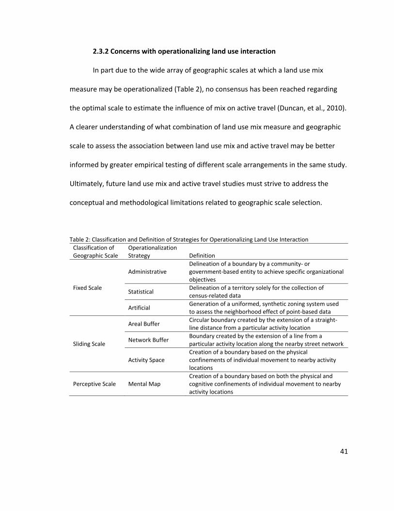
41

2.3.2 Concerns with operationalizing land use interaction

In part due to the wide array of geographic scales at which a land use mix

measure may be operationalized (Table 2), no consensus has been reached regarding

the optimal scale to estimate the influence of mix on active travel (Duncan, et al., 2010).

A clearer understanding of what combination of land use mix measure and geographic

scale to assess the association between land use mix and active travel may be better

informed by greater empirical testing of different scale arrangements in the same study.

Ultimately, future land use mix and active travel studies must strive to address the

conceptual and methodological limitations related to geographic scale selection.

Table 2: Classification and Definition of Strategies for Operationalizing Land Use Interaction

Classification of Geographic Scale

Operationalization Strategy Definition

Fixed Scale

Administrative Delineation of a boundary by a community- or government-based entity to achieve specific organizational objectives

Statistical Delineation of a territory solely for the collection of census-related data

Artificial Generation of a uniformed, synthetic zoning system used to assess the neighborhood effect of point-based data

Sliding Scale

Areal Buffer Circular boundary created by the extension of a straight-line distance from a particular activity location

Network Buffer Boundary created by the extension of a line from a particular activity location along the nearby street network

Activity Space Creation of a boundary based on the physical confinements of individual movement to nearby activity locations

Perceptive Scale Mental Map Creation of a boundary based on both the physical and cognitive confinements of individual movement to nearby activity locations

42

2.3.2.1 Conceptual concerns

A predominant theme in past studies into the association between land use mix

and active travel has been the absence of strong conceptual deliberation to inform the

choice of a geographic scale to operationalize any measure. Past adoptions of a fixed

geographic scale to study the neighborhood effect of land use mix on active travel have

likely been the result of analytical convenience or the availability of relatable

information on the sociodemographic and housing attributes at the selected scale.

Nevertheless, the choice of a fixed geographic scale as an operational unit to measure

land use mix must be accepted as a decision without any theoretical connection to

travel behavior (Guo & Bhat, 2007). As for the use of a sliding scale to operationalize

land use mix, the practice of using a quarter-, half-, or one-mile buffer distance has been

the standard for defining a feasible pedestrian environment. However, the continued

use of these spatial extents has been done so with little acknowledgement to the idea

that an active travel trip may differ by purpose and context (Schlossberg, 2006). Another

conceptual concern with the use of a sliding geographic scale has been the assumption

of an individual placed at the center of the scale having directionally invariant and

complete knowledge of the built environment influence surrounding their activity

locations or travel routes (Mitra & Buliung, 2012). In all, the conceptualization of a

neighborhood boundary with the selection of a geographic scale has remained a

conceptual dilemma facing researchers who study the association between local built

environment effects and active travel outcomes (Gauvin, et al., 2007).

43

A second and related conceptual shortcoming ubiquitous in present travel

behavior studies has involved the measurement of local land use mix or any

neighborhood effect of the built environment at a single scale and spatial extent for all

travel modes and purposes. Given the fact that any built environment measure will be

sensitive to the selected geographic scale, a possibility exists that different strategies for

operationalizing the built environment will only be relevant for certain trip contexts (Fan

& Khattak, 2008). For instance, the choice of a certain combination of scale category and

size may not represent the best strategy for measuring the effect of all built

environment measures (Lee & Moudon, 2006b). In turn, the selection of the most

relevant scale for operationalizing the built environment will likely depend on the travel

aspect under examination. The travel time budget of an individual conducting a

discretionary trip may be greater than that of an individual commuting, which may lead

the former individual to potentially be influenced by a wider set of land use types within

a larger activity space. As such, an administrative boundary may be more appropriate to

measure the influence of land use mixing on commuting. Work-related travel may more

likely be linked to the influences of a metropolitan region than a local geographic scale

describing the activities of a neighborhood; whereas, a nonwork trip may be heavily

influenced by the local land use patterns that induce active travel behaviors (Hong, et

al., 2013). Moreover, the use of a larger geographic scale or spatial extent in the latter

context may be too large to distinguish a pedestrian-oriented neighborhood from those

neighborhoods that are not (Ewing, et al., 2003).

44

2.3.2.2 Methodological concerns

The last point has also underscored a methodological limitation pertaining to

past efforts of measuring the association between land use mix and active travel

behavior. The geographic scale at which land use mix or other built environment

information are available to a researcher has typically determined the unit of analysis.

Past studies have simply relied on the best available data, which may be compiled from

a variety of unrelated sources and aggregated to a geographic scale inconsistent with

the study’s context (Ewing, et al., 2003). In considering the measurement of only the

built environment elements that matter to a traveler, the operationalization of land use

mix at a large fixed geographic scale will likely dilute the importance of land use mix on

active travel by averaging out influential land use patterns with surrounding land use

types not factoring into an individual’s travel decision (Guo & Bhat, 2007). Along the

same lines, past sliding geographic scale applications, which have sought to only

measure land uses in close proximity to the traveler, have failed to consider any

impedance aside from network distance. In actuality, additional objective factors related

to the physical environment, modal travel time, and traffic safety should also be

considered as constraints on the land use types that factor into an individual’s travel

decision.

The modifiable areal unit problem (MAUP) has been a well-established

methodological concern impacting the choice to use a fixed or sliding geographic scale

to analyze the land use mix and active travel connection. Fotheringham and Wong

45

(1991) described the MAUP as being the sensitivity of analytical results to the definition

of a geographic scale at which any spatial data are collected. Built environment data

have been collected to understand their association with another non-modifiable entity

such as an individual traveler, but the built environment effect has been reported at an

arbitrary and modifiable scale without any intrinsic spatial meaning to the individual or

land use. As such, geographic scale selection has reflected a subjective exercise of the

researcher seeking to aggregate non-modifiable entities (Openshaw, 1983). Since the

MAUP has been defined as a dilemma related to the selection of geographic scale and

analytical unit, any evaluation of travel behavior must give careful consideration to

these facets (Horner & Murray, 2002). However, disparity in the geographic scales

previously used within the literature have complicated the debate of how best to

operationalize land use mix for active travel research (Clark & Scott, 2014). This is

because such variation in geographic scale selection has increased the likelihood that

the MAUP has impacted the findings of previous studies using conventional land use mix

measures (Hess, et al., 2001).

Evaluating the impact of the MAUP on active travel behavior may be divided into

scale and zoning effects. The level of aggregation used to measure the built

environment has defined the former effect, while the configuration of a geographic

scale system has defined the latter (Fotheringham & Wong, 1991). Variations in the size

of geographic scale have resulted in a scale effect on analytical results (Mitra & Buliung,

2012) in which inconsistent findings are attributed to the operationalization of land use

46

mix at different scales for the same travel outcome (Hong, et al., 2013). Additionally,

alterations to the geographic scale that built environment data were originally collected,

which is considered the basic spatial unit for measuring the spatial phenomena, have

produced inconsistent results related to the representation of mix with an unintended

zonal arrangement (Mitra & Buliung, 2012). Despite a long-standing recognition of the

scale and zoning effect in the geography literature, the MAUP has received far less

attention in research examining the built environment and active travel relationship.

Future research would benefit from the use of multiple geographic scales to

operationalize land use mix and a reporting of the estimation results assessing the

association between active travel behavior and land use mix measured at varying

geographic scales (Mitra & Buliung, 2012).

The uncertain geographic context problem (UGCP) has more recently been

presented as a concern for operationalizing the built environment with implications for

future active travel research. As previously described, the identification of a suitable

geographic scale or spatial context for measuring the importance of land use mix or any

exposure measure has been an essential task for studying its effect on active travel

behavior (Kwan, 2013). The UGCP has stated that empirical results from studies using

area-based measures such as land use mix have been impacted by deviations in the

choice of geographic scale from the true geographic context of the phenomenon’s

influence on a studied travel behavior (Kwan, 2012). The past operationalization of land

use mix at a fixed or sliding geographic scale has introduced some spatial and temporal

47

uncertainty to any empirical finding, which may be methodologically addressed by the

adoption of a perceptive geographic scale. Spatial uncertainty has arisen from the belief

that little is known about the actual geographic scale that exerts a contextual influence

on the individual traveler, while the lack of knowledge about the timing and duration of

these contextual influences on travel has resulted in temporal uncertainty regarding the

application of fixed or sliding scale to operationalize land use mix (Kwan, 2012).

2.4 Temporal Availability

Time is a fundamental concept to the study of the transportation-land use

connection since an individual’s ability to both access and participate in an activity at a

given location is shaped by the temporal availability of that opportunity (Kwan, 2013).

Since travel demand derives from the requirement of an individual to partake in an out-

of-home activity, any variation in the surrounding land use supply (e.g., temporal

availability) will to some extent impact an individual’s revealed travel behavior (McNally

& Kulkarni, 1997). Accordingly, the failure to account for the temporal availability of a

land use (e.g., facility opening hours), a proxy for activity opportunity supply (Yoon &

Goulias, 2010), has embodied a clear conceptual and methodological omission of past

measures created to estimate the neighborhood effect of land use mixing on active

travel decisions. An addition of temporal availability to a spatial land use mix measure

specified with consideration to the other components of land use mix and geographic

48

scale carries considerable promise as an innovative policy instrument to help guide the

adoption of new and established urban policies aimed toward encouraging active travel.

A proposal to include the temporal availability component in future land use mix

measures has drawn heavily from the study of time geography. An adoption of concepts

introduced by this geography subfield, which has informed recent activity-based travel

demand modeling approaches, has provided an adaptable framework for a systematic

description of the spatial-temporal nature of behavioral constraints faced by an

individual (Burns, 1979). Behavioral restrictions characteristic of this time geography

strategy for understanding activity participation have been summarized as the

capability, coupling, and authority constraints faced by a traveler (Hagerstrand, 1970). In

this framework, the consideration of the temporal availability of an activity or land use

represents a potential authority constraint to the behavior exhibited by a traveler, who

cannot feasibly access a temporally unavailable opportunity. In thinking about shopping

activity participation, an individual may only feasibly conduct this activity during the

opening hours of the establishment (Neutens, et al., 2007). Extending this illustration to

a land use mix metric, a land use serving as a proxy for this shopping activity would also

only influence travel behavior if temporally available to the individual; therefore, a

temporally unavailable land use should likewise not be considered in a metric evaluating

the impact of land use mixing on travel behavior.

Unfortunately, exposure measures such as land use mix have tended to ignore

the authoritative role of temporal availability when examining the influence of

49

environmental determinants on individual travel behavior (Kwan, 2013). As such,

empirical evidence reflecting any discrepancies in the temporal availability of different

activity opportunities has been extremely scarce to date (Neutens, et al., 2011).

Unsatisfactory consideration to the temporal availability of different opportunities,

identified as the varying patterns of opening hours exhibited by different activity or land

use types, has led to a static, timeless representation of the built environment’s effect

on travel (Kwan & Weber, 2003). Pioneering research into the creation of an

accessibility measure sensitive to the opening hours of an urban activity has highlighted

that past accessibility measures without a temporal availability component have likely

produced inflated findings by assuming all activities to be available at all times of the

day (Weber & Kwan, 2002). As such, research supporting the creation of spatial-

temporal built environment measures has been described as being sorely needed;

especially, empirical study into the effect of spatial-temporal measures on active travel

behavior (Kim & Kwan, 2003). A statement for future analyses to identify the temporal

patterns and spatial complementarity of different activity types was previously stressed

by Goodchild & Janelle (1984).

An extension of this constraint-based time geography approach to measuring

activity accessibility holds considerable promise in providing a more thorough

understanding of the association between land use mix and active travel behavior.

Recent studies have adopted a spatial-temporal accessibility approach because of its

sensitivity to temporal behavioral constraints such as the opening hours of an

50

opportunity (Neutens, et al., 2011). Yet, to-date, the limited application of these spatial-

temporal strategies has almost exclusively focused on activity participation demand and

would greatly benefit from a greater descriptive understanding of the temporal supply

of land use patterns around an activity opportunity (Yoon & Goulias, 2010; Yoon, et al.,

2014). Increased availability of disaggregate built environment data coupled with recent

computational advancements has enabled the introduction of a spatial-temporal

measure capable of representing complexities related to the temporal availability of

certain land uses (Kwan & Weber, 2003).

2.4.1 Representing temporal availability

Recalling the typology of land use mix measures, the temporal availability

component has only been studied in measures of accessibility. Explicit attention to the

temporal availability of an activity location to an individual traveler in an accessibility

measure has the potential to provide a higher quality time-space representation of the

feasible opportunities available to an individual and, therefore, benefit the predictions

of his/her travel behavior (Chen, et al., 2011). Traditionally, access to an activity location

has been treated as a static temporal assumption with minimal acknowledgment to the

diurnal variability of service provisions (Neutens, et al., 2012). However, the persistent

application of accessibility measures with this static time assumption have marginalized

the reality that these activity locations have specific temporal schedules or opening

hours rendering them unavailable to a traveler at certain hours of the day (Landau, et

51

al., 1982; Kwan, 2013). A failure to accommodate these temporal schedules in an

accessibility measure has additionally led to overestimations of an individual’s activity

space (Schwanen & Jong, 2008). A comprehensive understanding of the spatial and

temporal arrangement of activities related to the feasibility for individual travel

between available opportunities in addition to an individual’s response to the built

environment constraints has symbolized two key facets to any accessibility metric (Pirie,

1979). Accordingly, formation of an accessibility measure capturing the spatial-temporal

availability of activity opportunities and the constraints shaping individual behaviors has

the capability for advancing present understandings of how the built environment

influences travel behavior (Yoon, et al., 2014).

2.4.1.1 Known temporal availability in accessibility measures

Intuitively, the most direct strategy for accurately representing temporal

availability within an accessibility measure has been to collect and incorporate data

pertaining to the opening hours of an establishment. However, the collection of high-

quality temporal availability data has remained costly and time consuming (Kwan,

2013); thus, hindering the adoption of this strategy. Applying a constraint-based

approach to analyzing joint trip making, Neutens et al. (2007) proposed the creation of a

spatial-temporal accessibility measure in which the analysis concentrated on the

facilities in which opening hours were identified. The temporal availability of these

52

facilities may then be aggregated into any time interval to establish the area of an

individual’s activity landscape for a specified time period (Neutens, et al., 2012).

While an encouraging strategy for incorporating temporal availability into future

measures, the limitation of data availability has confined past analyses to only explore a

select set of facilities. Schwanen and Jong (2008) integrated the known temporal

availability of daycare centers in Utrecht, the Netherlands to examine the impact of

opening hours on the commuting behavior of one exemplar mother. Meanwhile,

Delafontaine et al. (2011) collected information on the opening hours of 16 libraries in

Ghent, Belgium to create a spatial-temporal measure of individual accessibility for use in

an equity context. Until data on the known temporal availability of more business types

become more readily available, future accessibility studies will be limited in the diversity

of businesses they may analyze. A potential strategy for improving the variety of

business with known temporal availability would be to collect complementary land use

and business data when designing and conducting new activity-travel household surveys

(Chen, et al., 2011). The collection of these data would further enable the creation of a

temporal availability taxonomy for different activity or land use types (Yoon, et al.,

2014).

2.4.1.2 Assumed temporal availability in accessibility measures

A second strategy for reflecting temporal availability in a spatial-temporal

accessibility measure has been to fix an assumed opening hour schedule on all facilities.

53

In the assumed temporal availability strategy, all facilities or those providing a similar

service are assigned identical opening hours (Neutens, et al., 2011). In exploring the

effect of geographic scale variability on individual accessibility, Kwan and Weber (2008)

utilized a spatial-temporal accessibility measure based on the assumption of a prior

study (Weber & Kwan, 2002) that all commercial and industrial opportunities were only

temporally available from 6:00 am to 9:00 pm. In the latter study, an accessibility

measure sensitive to temporal availability displayed significant variation across several

fixed geographic scales. Refinements to this assumption have been made in other

studies (Kim & Kwan, 2003), where an industrial opportunity was assumed to only be

temporally available from 9:00 am to 5:00 pm, but a commercial opportunity was

available from 9:00 am to 9:00 pm. While an assumed temporal availability

representation in an accessibility measure marks an improvement over no account of

temporal variability, Delafontaine et al. (2011) noted their use of known temporal

availability highlighted significant differences in the distribution of opening hours among

facilities of the same regime in both times of the day and days of the week.

2.4.1.3 Activity-related temporal availability in accessibility measures

Recent research has presented a strategy for measuring temporal availability

acknowledging the difficulty of collecting existing opening hour data as well as the

shortcomings of an assumed temporal availability strategy for measuring accessibility.

Chen et al. (2011) introduced an activity-related strategy in which the revealed activity

54

arrival and departure times of an individual were used to assign a weighted percent of

reachable workers per time interval for various establishments. In this activity-related

strategy, a certain business type has been considered temporally available to an

individual traveler if any employee for that specific industry was observed to be

performing a work-related activity during that time period. By using revealed household

travel survey data, an intensity of different opportunity types has been determined

through the imputation of temporal availability data based on individual activity

participation (Yoon, et al., 2014). Initial analyses using this strategy have discovered the

arrival time of an individual to a facility may be a more accurate reflection of activity

temporal availability than the departure time of an individual from his/her last activity

(Yoon, et al., 2012).

While an exciting prospect for generating a temporally-sensitive dataset when

the collection of known temporal availability data is unachievable, an adoption of an

activity-related strategy for measuring accessibility has several limitations. Dependence

on a standardized system of business classifications may be insufficient as a proxy of the

actual land use of an establishment, which could potentially have several functions

(Yoon, et al., 2014). Similarly, the use of revealed activity arrival and departure times

from survey respondents may be an inadequate proxy for deriving the temporal

availability of an establishment that should be compared to external data sources when

known temporal availability data become available (Chen, et al., 2011). Moreover,

future accessibility research should consider advancements to the realism of an activity-

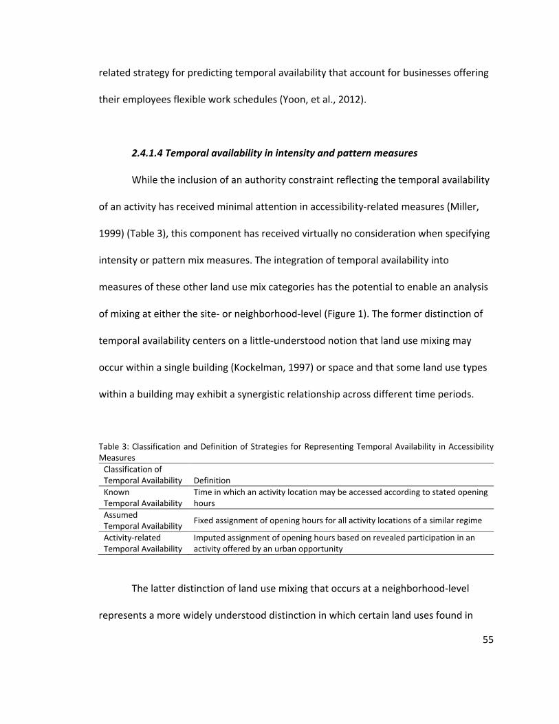
55

related strategy for predicting temporal availability that account for businesses offering

their employees flexible work schedules (Yoon, et al., 2012).

2.4.1.4 Temporal availability in intensity and pattern measures

While the inclusion of an authority constraint reflecting the temporal availability

of an activity has received minimal attention in accessibility-related measures (Miller,

1999) (Table 3), this component has received virtually no consideration when specifying

intensity or pattern mix measures. The integration of temporal availability into

measures of these other land use mix categories has the potential to enable an analysis

of mixing at either the site- or neighborhood-level (Figure 1). The former distinction of

temporal availability centers on a little-understood notion that land use mixing may

occur within a single building (Kockelman, 1997) or space and that some land use types

within a building may exhibit a synergistic relationship across different time periods.

Table 3: Classification and Definition of Strategies for Representing Temporal Availability in Accessibility Measures

Classification of Temporal Availability Definition

Known Temporal Availability

Time in which an activity location may be accessed according to stated opening hours

Assumed Temporal Availability

Fixed assignment of opening hours for all activity locations of a similar regime

Activity-related Temporal Availability

Imputed assignment of opening hours based on revealed participation in an activity offered by an urban opportunity

The latter distinction of land use mixing that occurs at a neighborhood-level

represents a more widely understood distinction in which certain land uses found in

56

close proximity may exhibit a synergistic relationship within the same time period. This

representation of land use mix reflects the established ideal of smart growth supporters

in which certain land uses (e.g., residence, market) may be integrated more

harmoniously than other blends if the intention is to induce active travel outcomes.

Current intensity and pattern measures inflate the neighborhood-level of land use

mixing by not accounting for the temporal availability of activity locations. For instance,

a grocery store located in close proximity to an individual’s residence may not be

accessible to that individual if his/her out-of-home activity schedule excludes them from

accessing the market during its opening hours (Kwan, 2013).

2.4.2 Benefits of representing temporal availability

Beyond its clear conceptual contribution, the incorporation of temporal

availability in future land use mix measures may be translated into practical benefits

related to the support of transportation-land use policies, identification of social

inequities in spatial-temporal accessibility, and improvement of travel demand behavior

modeling. Built environment measures representing temporal availability have direct

implications on transportation policies affecting local communities (Neutens, et al.,

2011). Portland Metro has proposed an activity level hierarchy (14-hour, 18-hour, and

24-hour) for select neighborhoods based on residential population, business activity, the

built environment, and transportation options (Metro, 2011); however, the activity

spectrum has not been supported by any empirical-based measure with sensitivity to

57

temporal availability. A measure sensitive to the temporal availability of land use types

may help direct active travel initiatives seeking to bring functional origin and destination

pairings closer to one another. Relatedly, an identification of the precise blend of land

use types needed for an efficient spatial-temporal distribution of activity locations

informed by a spatial-temporal land use mix measure may help guide infill or new

development projects and more precisely model the active travel implications.

Figure 1: Illustration of Site- and Neighborhood-Level Temporal Availability of Mixing Land Use Types

In addition to an improvement in neighborhood design efficiency, adoption of a

spatial-temporal measure holds potential toward informing the management of

businesses considering an extension of opening and closing hours (Yoon, et al., 2014).

The liberalization of opening hours may enable individuals to conduct activities outside

58

standard business hours; subsequently, providing individuals with an ability to combine

out-of-home activities and improve their prospects for trip chaining (Neutens, et al.,

2011). Also, an inclusion of the temporal availability component in future measures will

improve the instruction of shared-parking arrangements in which a parking structure

used by the employees of an office building during the day may be used in the evening

by drivers accessing entertainment opportunities (Cervero, 1996). For each application,

research is needed to enhance the capability of temporally sensitive measures to inform

transportation planning and practice (Neutens, et al., 2011).

Another exciting prospect from the standpoint of active travel research is the

consideration of the spatial-temporal accessibility inequities faced by individuals who

rely on active travel modes (Neutens, et al., 2012). An account of the temporal

availability of urban opportunities offers significant insight into the ways that certain

individuals or market segments may be affected by variations in the opening hours of

facilities found within a neighborhood (Weber & Kwan, 2002). Thus, the creation of a

land use mix metric accounting for temporal availability has an ability to evaluate how

different opening hour configurations for certain types of services may benefit or hinder

those individual disparities that exist in a metropolitan region for accessing basic human

services (Delafontaine, et al., 2011). Without consideration for temporal constraints

such as opening hours, conventional mix measures have remained insensitive to

fluctuations in the availability of certain activities over the course of a day or week. A

59

consequence of this mismatch between the need for activity engagement and temporal

availability of the activity may be social exclusion (Neutens, et al., 2011).

Finally, specification of a land use mix measure incorporating an authority

constraint will improve activity-based travel demand models, which have to-date largely

concentrated on the coupling constraint of individuals within a household interacting

with one another (Yoon & Goulias, 2010). By disregarding the temporal availability of

certain activities or land uses, present models may underestimate the demand for

conducting certain activities and in turn distort future travel demand patterns by poorly

allocating where activities may occur in the future (Kwan, 2013). For that reason and

others, the representation of spatial-temporal travel decisions and the built

environment factors influencing activity participation must be better understood within

future activity-based travel research (Yoon, et al., 2014). The creation of a

comprehensive land use mix measure accounting for the temporal availability of specific

land use types helps to fulfill this request.

2.5 Synthesis

Future measures must improve how the land use mix and geographic scale

components of the construct are represented, while introducing the temporal

availability component. The prior sections of this literature review have identified each

component and discussed the conceptual and methodological concerns hampering

these three interrelated components of a spatial-temporal land use mix measure. As

60

detailed disaggregate data and improved technologies become increasingly available to

researchers, the importance to advance constructs related to each of these land use mix

components will become ever more important to understanding the true association

between land use mix and active travel behavior. Urban planning and public health

researchers interested in the adoption of land use mix policies must continue to

challenge the adoption of flawed measures in order to provide decision makers with a

more astute assessment of how increased local land use mixing relates to active travel.

Table 4 synthesizes the strategies for representing each component of a spatial-

temporal land use mix measure and rates the conceptual and operational complexity of

adopting each strategy.

Table 4: Conceptual and Operational Complexity of Representing the Strategies for each Land Use Mix Component

Land Use Mix Component Strategy for Representing Land Use Mix Component

Land Use Interaction Accessibility Intensity Pattern Geographic Scale Fixed Sliding Perceptive Temporal Availability Known Assumed Activity-related

Complexity Level Low Moderate High

61

Chapter 3: An Activity-Related Land Use Mix Construct and its Connection to

Pedestrian Travel

3.1 Introduction

The sustained popularity for transportation-land use interactions investigation

over the past three decades has fundamentally shaped modern planning scholarship

(Boarnet, 2011). Attraction for research in this sub-discipline emerges from a prospect

for planners to moderate travel behavior by physically altering the urban landscape

(Ewing & Cervero, 2010). Studies into this central principle of the transportation-land

use connection generally accept that a compact neighborhood characterized by a

diversity of activity destinations and traditional street network design supports

pedestrian travel (Cervero & Kockelman, 1997). A recognition evidenced by the growing

adoption of transportation-land use strategies by local, regional, and state agencies;

whose guiding visions and programs emphasize the many purported transportation,

land use, and public health benefits related to neighborhood land use mixing.

From a transportation perspective, smart growth policies intended to increase

local land use mixing bring functional origins and destinations closer; therefore,

decreasing trip distances and making walking competitive with faster travel modes

(Clifton, et al., 2008). Land use mixing is also viewed as a strategy for balancing travel

demand uniformly across the day (Cervero, 1996), promoting trip chaining (Maat &

Timmermans, 2006), and reducing vehicle distance traveled, mode selection, and

62

ownership (Cervero, 1989; Kockelman, 1997). Viewed through a land use planning lens,

policies aimed at siting diverse land uses in a compact setting provide a visibly

interesting built environment conducive to walking (Reilly & Landis, 2003; Forsyth, et al.,

2008). Stimulating mixed-use development also provides a policy instrument to

encourage urban revitalization and slow rural land consumption (Downs, 2005).

Public health researchers investigating the link between chronic disease risk

factors and the built environment also exude the benefits of smart growth policies

(Christian, et al., 2011; Wineman, et al., 2014). An intermixing of complementary land

use types provides neighborhood residents and visitors a diversity in destination types

that facilitates walking and physical activity (Forsyth, et al., 2008; Brownson, et al.,

2009). Other physical health benefits such as reduced vehicle emissions exposure

through congestion mitigation (Frank, et al., 2008) and mental health-related benefits

such as increased neighborly communication or an improved sense of place (Manaugh &

Kreider, 2013; Song, et al., 2013a) are also attributed to mixed-use landscapes.

Ultimately, multidisciplinary research has heralded land use mix as a planning

goal that policymakers must realize to form neighborhoods favorable to active, healthy

lifestyles (Duncan, et al., 2010). However, this connection between land use mix and

pedestrian travel remains complicated by the many measures chosen by researchers to

objectively illustrate this intangible environmental construct (Manaugh & Kreider,

2013). A division between research and practice resulting in the provision of measures

63

with imperfect theoretical foundations, which likely hinders the implementation of land

use mix as a performance metric in practice (Gehrke & Clifton, 2016).

This paper critiques current practice and introduces a land use mix measure

reflecting the composition and configuration of local land uses. Specifically, this study

depicts mix as a latent construct in which the ideal composition of local land use types is

guided by observed activity distributions and their spatial arrangement is explicitly

expressed. Statistically significant associations are found between the proposed land

use mix construct and pedestrian travel behaviors. Planners who wish to promote

walking may benefit from this conceptualization of land use mix.

3.2 Land Use Mix Measurement and Pedestrian Travel

Land use mix is aptly defined as the level of integration among different land use

types in a neighborhood (Saelens, et al., 2003). A succinct description that presents a

challenging array of choices to quantify the mixing of neighborhood land uses (Brown, et

al., 2009). Given this challenge and a recognition that mixed-use settings improve active

transport viability (Handy, 2005), land use mix has become the most frequently

evaluated built environment determinant of physical activity (Brownson, et al., 2009).

With this in mind, planners must be cognizant of how this environmental phenomenon

is operationalized to ensure that policy and practice are guided by empirical evidence

originating from proposed theory (Frank, 2000).

64

The theory supporting land use mix and the measurement of an ideal level of

integration among different land use types will likely vary based on the outcome of

interest. In this study of pedestrian travel outcomes, I was interested in operationalizing

land use mix as a construct grounded in travel behavior theory. The following

subsections, organized by the quantification of land use mix as a distance, intensity, or

pattern measure (Song & Rodriguez, 2005), offer a transportation-related conceptual

basis for adopting a measurement type and a review of pedestrian travel studies

exploring each dimension.

3.2.1 Distance measures

Accessibility is the ease of an individual to reach an opportunity from a given

activity location (Kwan & Weber, 2008). Operationalized as a mix measure, the

opportunity and activity locations are presented function-related land use designations,

while the ease of travel between locations is customarily conveyed as distance. A

resulting metric quantifies the spatial arrangement of two land uses as the relative

burden of traveling between them (Clifton, et al., 2008). By reducing the distance

between locations, walking’s feasibility increases and the competitive edge of faster

travel modes diminishes.

Studying this connection between distance-based accessibility and walking,

Krizek and Johnson (2006) found individuals living within 200 meters of a retail

establishment were more likely to walk than residents living at least three times farther

65

from a similar land use. Conversely, Lee and Moudon (2006a) modeled a negative

association between proximity of mixed-use neighborhood centers and the likelihood to

walk; whereas, Reilly and Landis (2003) found a positive link between access to

commercial uses and this outcome. In a study of walk frequency, Shay et al. (2006)

discovered a shortened distance to a commercial center positively impacted utilitarian

travel. Other studies have noted the positive connection between grocery store

proximity and walk trip frequency (Handy & Clifton, 2001; Cao, et al., 2006; Handy, et

al., 2006).

In general, studies of distance-based accessibility and walking support the

hypothesized transportation-land use connection. However, while quantifying mix as a

distance-based measure is conceptually simple, its adoption as an area-based summary

is empirically limited (Brownson, et al., 2009). Distance measures provide insufficient

detail by only measuring the spatial proximity of two activity locations, solely providing

a summary calculation for the origin, and failing to quantify the quality of the described

link.

3.2.2 Intensity measures

Intensity measures quantify the frequency or percent of activity locations in a

landscape dedicated to a specific land use type (Brownson, et al., 2009; Song, et al.,

2013a). A count of land use types is a proxy for how many potential trip origins or

destinations exist within a neighborhood (Hess, et al., 2001), while a percent explains

66

the scarcity or dominance of an activity type (Song, et al., 2013a). Both the frequency

and size of activity locations, or land uses, contribute to neighborhood accessibility and

the increased willingness of an individual to walk for activity fulfillment (Handy, 1993).

Studying the environmental determinants of physical activity, Hoehner et al.

(2005) discovered that residents with a high intensity of nonresidential destinations

within a quarter-mile of their home had an increased propensity for walking. Specifying

a single activity type, Frank et al. (2007) and Boarnet et al. (2011) found an increased

intensity in recreational spaces and retail stores, respectively, increased this likelihood

to walk. Kerr et al. (2007) noted the nearby presence of a recreational or commercial

land use impacted youth walk mode choice. Exploring its connection to time spent

walking, past studies found an increased intensity of grocery stores, offices, retail shops,

and schools (Lee & Moudon, 2006a; McConnville, et al., 2010) and commercial

establishments (Nagel, et al., 2008) increased pedestrian travel. In a study of ten metro

regions, Boer et al. (2007) operationalized mix as the count of unique business types

within a neighborhood and discovered a positive relationship with distance walked.

Meanwhile, Forsyth et al. (2008) found the percent of area devoted to a social land use

positively predicted distance and time spent walking for subsistence and maintenance

trips.

Despite variation in the nonresidential land uses analyzed, a higher intensity of

out-of-home activity locations was commonly connected to increased pedestrian travel.

The conceptual link is straightforward: a greater intensity of nonresidential land uses

67

near an individual’s residence enhances the practicality of walking to daily life activities

by reducing travel distance (Handy, et al., 2002). However, mix as an intensity measure

is limited by its inability to summarize the count or percentage of multiple land uses as a

single value and sensitivity to spatial scale selection (Song, et al., 2013a).

3.2.3 Pattern measures

A final measurement category quantifies mix as the composition and

configuration of local land use types. In transportation-land use study, land use mix as a

pattern measure has exclusively been measured as the composition, or distribution, of

different land use types in a neighborhood (Frank & Pivo, 1994). A neighborhood with a

mixture of both residential and nonresidential land uses influences travel demand by

inducing internal walk trips that substitute for prospective out-of-neighborhood

motorized trips (Cervero & Kockelman, 1997). Regularly, a version of the land use

entropy index, introduced to planning research by Cervero (1989), has summarized the

degree of mixing in an area.

Analyzing the built environment determinants of travel in 15 regions, Ewing et al.

(2015) found an increase in the entropy score of three land use types (residential,

commercial, and public) within a quarter-mile of the traveler’s residence positively

predicted walk mode choice. Earlier, Zhang and Kukadia (2005) discovered the balance

of residential, commercial, and industrial land uses near a residence became a stronger

predictor of walking as the spatial extent of operationalization increased. Summarizing

68

the evenness amongst these same three land uses, Wineman et al. (2014) discovered a

negative link with time spent walking; whereas, Rajamani et al. (2003) modeled a

positive link with walk mode choice for nonwork travel when a fourth class reflecting all

other land uses was incorporated. Frank et al. (2008) echoed this latter finding in a

Seattle-based study associating the entropy score of residential, office, retail, and

entertainment land uses with walk mode choice. A previous study (Frank, et al., 2004)

summarizing the balance of residential, office, commercial, and institutional land uses in

Atlanta neighborhoods found increased evenness predicted distance walked. Studying

active travel in San Francisco, Cervero and Duncan (2003) generated a land use diversity

factor indicated by residential, office, retail, and industrial balance at the trip origin and

found the factor positively predicted the decision to walk.

This evidence and prior reviews (Saelens & Handy, 2008; Brownson, et al., 2009)

mostly support a positive relationship between entropy-based indices and pedestrian

travel. However, evenness is often depicted as land use mix despite only summarizing a

landscape’s composition of land use types and not their spatial arrangement. As a

result, neighborhoods with considerably different configurations of land use types can

produce identical entropy scores (Hess, et al., 2001; Manaugh & Kreider, 2013). Further,

a neighborhood with an entropy score of one is assumed to embody an ideal level of

land use mixing for travel; yet, no theoretical foundation links an equal balance of all

land use types with demand (Rodriguez, et al., 2009, Song, et al., 2013a). Since land use

mix is intrinsically a spatial phenomenon, an apt depiction must not only measure the

69

diversity of land use types in a neighborhood, but also convey the configuration of these

parcels. Relatedly, entropy indices typically fail to consider the functional

complementarity amongst the assessed land use types. A consequence of these

oversights has been the adoption of theoretically flawed measures of composition and

inattention to the pattern aspect of configuration. By measuring land use mix based on

composition and configuration, a more robust investigation of this environmental

phenomenon and its theorized link to pedestrian travel will be achieved (Hess, et al.,

2001).

3.3 Land Use Composition and Configuration

Spatial heterogeneity describes the complexity in composition and configuration

of landscape patches. In landscape ecology, composition is the number of land use

patches or proportion of each type, while configuration reflects the spatial

arrangement, shape, and dissimilarity of landscape patches (Li & Reynolds, 1994;

Turner, 2005). The field is founded on the notion that these paired pattern aspects

comprise landscape structure, which in turn strongly impact behavioral processes

(McGarigal & McComb, 1995). Rather than defining urban development patterns, the

motivation of landscape ecology research has centered on understanding how these

aspects inform environmental protection and resource conservation (Clifton, et al.,

2008). Consequently, interest in the quantification of spatial heterogeneity has

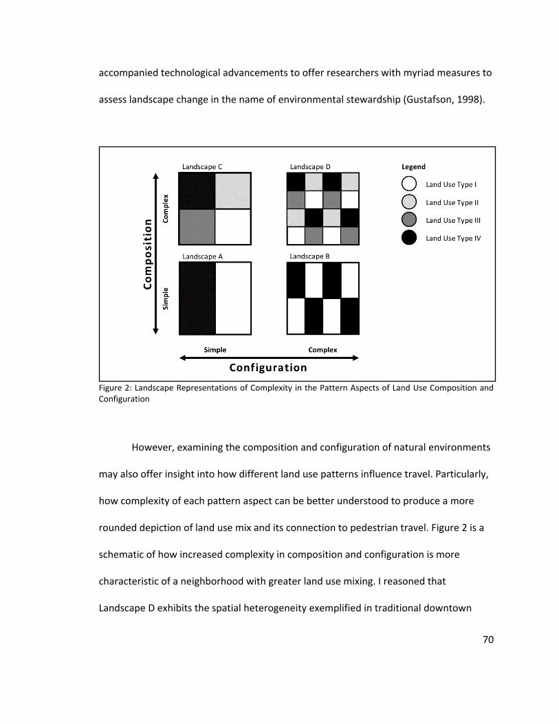
70

accompanied technological advancements to offer researchers with myriad measures to

assess landscape change in the name of environmental stewardship (Gustafson, 1998).

Figure 2: Landscape Representations of Complexity in the Pattern Aspects of Land Use Composition and Configuration

However, examining the composition and configuration of natural environments

may also offer insight into how different land use patterns influence travel. Particularly,

how complexity of each pattern aspect can be better understood to produce a more

rounded depiction of land use mix and its connection to pedestrian travel. Figure 2 is a

schematic of how increased complexity in composition and configuration is more

characteristic of a neighborhood with greater land use mixing. I reasoned that

Landscape D exhibits the spatial heterogeneity exemplified in traditional downtown

71

settings celebrated for their intermingling of diverse activity locations (Cervero, 1989),

which best supports walking.

To date, planning research has almost entirely studied the travel outcomes of

mixed-use development patterns by employing measures insensitive to spatial

arrangement. An unintended result has been the implementation of mix measures that

imperfectly reflect the increased intensity, diversity, and integration of land use types

described by urban form theory as sustainable land development (Grant, 2002). In

response, this study aims to (a) provide planners with a land use mix measure

quantifying land use composition and configuration, and (b) demonstrate the link

between this multifaceted construct and pedestrian travel.

3.4 Study Area and Land Use Data

This study examines the interactions between landscape pattern and walking

within six counties located in Oregon’s Willamette River Valley. An expansive area was

chosen to capture variations in landscape and travel patterns found across the three

metro regions of Portland, Salem, and Eugene. Portland is the population and economic

hub of the study area with a metro region reaching into Multnomah, Washington, and

Clackamas counties. Salem is the state capitol located in Marion and Polk counties, and

Eugene is located entirely in Lane County. Each urbanized area is enclosed by a state

mandated growth boundary controlling expansion and promoting efficient development

patterns.

72

Table 5: Distribution of Parcels Categorized with the Land-Based Classification Standard (LBCS)

LBCS Code Land Use Function Parcels Area (Sq. Miles)

1000 Residence or accommodation

694,752 (76.82%)

306.48 (3.24%)

2000 General sales or services

35,418 (3.92%)

63.80 (0.68%)

3000 Manufacturing and wholesale trade

11,339 (1.25%)

94.83 (1.00%)

4000 Transportation, communication, information, and utilities

2,425 (0.27%)

69.17 (0.73%)

5000 Arts, entertainment, and recreation

8,740 (0.97%)

317.02 (3.35%)

6000 Education, public administration, health care, and other institutions

14,630 (1.62%)

273.73 (2.90%)

7000 Construction-related businesses

1,211 (0.13%)

1.39 (0.01%)

8000 Mining and extraction establishments

194 (0.02%)

15.89 (0.17%)

9000 Agriculture, forestry, fishing and hunting

125,065 (13.83%)

7,606.96 (80.48%)

undefined N/A

10,624 (1.17%)

702.18 (7.43%)

904,398 9,451.45

To measure land use type composition and configuration in landscapes across

the six counties, collection of a universal parcel dataset and adoption of a standardized

classification scheme was paramount. Parcel-level data with linked property attributes

were provided by the metropolitan planning organizations, who maintained these

spatial data sources shared by county assessment and taxation offices. Data were

amassed in a Geographic Information System and discrepancies in land use type

assignment were reconciled using the property classification established for each tax lot

by the Oregon Department of Revenue. After property code identification, all parcels

were assigned one of nine land use function codes in accordance to the American

Planning Association’s Land-Based Classification Standards (Table 5). Finally, the study

area was delineated into 65,312,000 66-foot grid cells, which standardized the unit of

73

analysis to approximate the smallest land parcels. Each artificial grid cell was assigned a

land use classification based on the underlying tax lot information.

3.5 Land Use Mix Indicators and Construct Measurement

A set of land use mix indicators centered on the aforementioned theoretic principles

of composition and configuration were calculated using these land use data. Each

indicator was operationalized at a one-quarter, one-half, and one-mile grid cell extent to

help understand variation in the neighborhood effects of land use mixing. A land use

mix construct was then measured using the resulting indicators.

3.5.1 Land use mix indicators

3.5.1.1 Land use composition

A core set of composition metrics assess the number of land use categories,

relative proportion of each category, and diversity amongst chosen categories

(Gustafson, 1998). Translated to a planning context, the first two sets of metrics assess

the count or percent of parcels in a neighborhood dedicated to a particular land use

type; whereas, diversity is a function of both the intensity and distribution of land use

types in a landscape. To ensure composition was reflected in the land use mix construct,

two indicators of diversity, grounded in planning theory, were calculated.

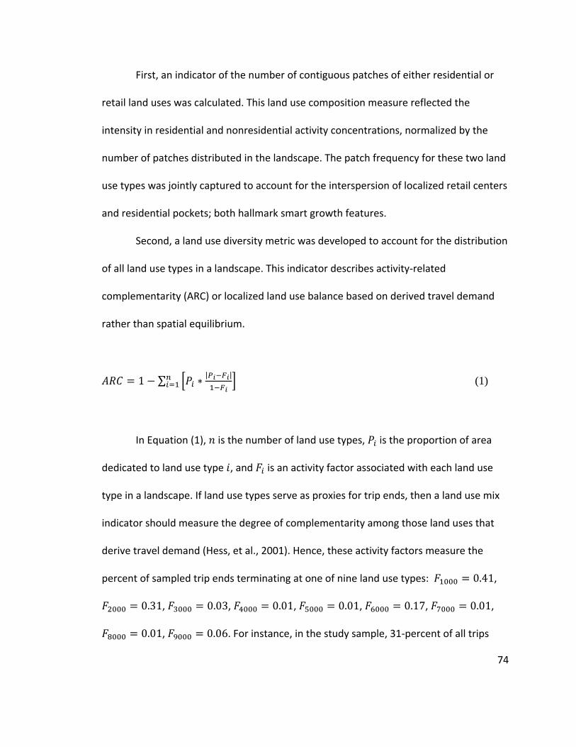
74

First, an indicator of the number of contiguous patches of either residential or

retail land uses was calculated. This land use composition measure reflected the

intensity in residential and nonresidential activity concentrations, normalized by the

number of patches distributed in the landscape. The patch frequency for these two land

use types was jointly captured to account for the interspersion of localized retail centers

and residential pockets; both hallmark smart growth features.

Second, a land use diversity metric was developed to account for the distribution

of all land use types in a landscape. This indicator describes activity-related

complementarity (ARC) or localized land use balance based on derived travel demand

rather than spatial equilibrium.

𝐴𝑅𝐶 = 1 − ∑ [𝑃𝑖 ∗|𝑃𝑖−𝐹𝑖|

1−𝐹𝑖]𝑛

𝑖=1 (1)

In Equation (1), 𝑛 is the number of land use types, 𝑃𝑖 is the proportion of area

dedicated to land use type 𝑖, and 𝐹𝑖 is an activity factor associated with each land use

type in a landscape. If land use types serve as proxies for trip ends, then a land use mix

indicator should measure the degree of complementarity among those land uses that

derive travel demand (Hess, et al., 2001). Hence, these activity factors measure the

percent of sampled trip ends terminating at one of nine land use types: 𝐹1000 = 0.41,

𝐹2000 = 0.31, 𝐹3000 = 0.03, 𝐹4000 = 0.01, 𝐹5000 = 0.01, 𝐹6000 = 0.17, 𝐹7000 = 0.01,

𝐹8000 = 0.01, 𝐹9000 = 0.06. For instance, in the study sample, 31-percent of all trips

75

terminated at a location providing general sales or services. The term |𝑃𝑖 − 𝐹𝑖| defines

the absolute difference between the landscape area dedicated to land use type 𝑖 and

the observed trip attraction for activities located at land use type 𝑖. Further dividing the

absolute difference by 1 − 𝐹𝑖 produces a ratio emphasizing land use types with higher

observed levels of travel demand and deemphasizing those with less. The resulting ratio

is then multiplied by 𝑃𝑖 to adjust it by the observed spatial proportion of the land use

type.

Akin to an entropy index score, this pattern metric ranges in value from zero to

one. A score of zero indicates a landscape dominated by a single land use type; whereas,

a score of one indicates a landscape where the spatial allocation of all land use types

perfectly matches the observed attraction for activities. As such, a landscape with a high

proportion of residences and retail stores scores higher than a landscape with a high

proportion of land dedicated to agriculture or manufacturing.

3.5.1.2 Land use configuration

In complement to these composition measures are those spatial heterogeneity

measures of a landscape using patch- or pixel-based land use configuration indices

(Gustafson, 1998). A maximum patch size measure was calculated by determining the

largest area of adjoining parcels of a single land use and then normalizing this

calculation by overall landscape area. This indicator identified landscapes with high

patch aggregation or isolation, independent of the land use types in a landscape.

76

Finally, a pixel-based metric of patch disaggregation and interspersion specific to all land

use types was calculated. Landscape ecologists commonly apply a contagion index

(O'Neill, et al., 1988; Li & Reynolds, 1994) to differentiate landscapes with a small

number of contiguous patches from those with an intermixing of dissimilar patch types,

which characterizes a landscape with a high level of land use integration. (Clifton, et al.,

2008).

𝐶𝑜𝑛𝑡𝑎𝑔𝑖𝑜𝑛 𝐼𝑛𝑑𝑒𝑥 = 1 +∑ ∑ [(𝑃𝑖𝑗) ln(𝑃𝑖𝑗)]𝑛

𝑗𝑛𝑖

2 ln(𝑛) (2)

The numerator in Equation (2) is the entropy index adopted from information

sciences (Shannon & Weaver, 1949), where 𝑃𝑖𝑗 is the probability that two randomly

selected adjacent 66-foot grid cells in a landscape belong to patch type 𝑖 and 𝑗. As the

pixels in a landscape become more fragmented, the contagion index score nears a value

of zero. Although contagion index calculation is complicated by the construction of a

spatial dissimilarity matrix, this configuration metric provides a unique representation of

the neighboring land use contrasts in a landscape (Li & Reynolds, 1994).

Together, these four metrics reflect a parsimonious collection of independent

land use mix indicators. However, while landscape pattern may sufficiently be quantified

using a handful of chosen metrics, planners must be aware that indicators chosen to

reflect these unique aspects may be correlated (Leitao, et al., 2006). Table 6 provides a

77

summary for each land use mix indicator, operationalized at the three artificial grid

extents.

Table 6: Descriptive Statistics and Zero-Order Correlation Matrix of Indicators at Three Geographic Scales

Land Use Mix Indicator

Land Use Mix Indicator Mean SD Min Max 1 2 3 4

One-Quarter Mile Grid 1: Residential and Retail Patch Richness

0.032 0.116 0.000 1.000 ---

2: Activity-related Complementarity 0.049 0.151 0.000 0.941 0.769 --- 3: Maximum Patch Size 0.941 0.154 0.039 1.000 0.662 0.806 --- 4: Contagion Index 0.953 0.096 0.359 1.000 0.588 0.699 0.831 --- One-Half Mile Grid 1: Residential and Retail Patch Richness

0.036 0.112 0.000 1.000 ---

2: Activity-related Complementarity 0.070 0.179 0.000 0.924 0.756 --- 3: Maximum Patch Size 0.917 0.184 0.027 1.000 0.649 0.830 --- 4: Contagion Index 0.941 0.105 0.397 1.000 0.583 0.729 0.820 --- One Mile Grid 1: Residential and Retail Patch Richness

0.037 0.103 0.000 0.941 ---

2: Activity-related Complementarity 0.092 0.200 0.000 0.913 0.718 --- 3: Maximum Patch Size 0.891 0.211 0.028 1.000 0.638 0.853 --- 4: Contagion Index 0.926 0.112 0.398 1.000 0.590 0.763 0.816 ---

Note: An italicized value indicates a negative Spearman correlation value.

3.5.2 Land use mix measurement

Confirmatory factor analysis (CFA) was used to identify a latent construct

reflective of the paired pattern aspects of composition and configuration. The adoption

of a CFA framework provided a hypothesis-driven process for measuring relationships

between a set of observed indicators supported by a priori theory and evidenced to

reflect an underlying construct (Brown, 2006). Accordingly, informed by planning and

landscape ecology theory, a latent variable model was specified to identify a land use

mix construct supporting the interrelationships among four objective composition and

78

configuration indicators within a landscape. A landscape with high land use mixing is

hypothesized to reflect complexity in not only land use composition, but also spatial

configuration. Table 7 provides results of three CFA models, which were estimated at

varying spatial scales.

Table 7: Confirmatory Factor Analyses of Land Use Mix Operationalized at Three Geographic Scales

Land Use Mix Indicator B SE (B) β p

CFA Model 1: One-Quarter Mile Grid Residential and Retail Patch Richness 0.542 0.003 0.665 0.000 Activity-related Complementarity 0.909 0.004 0.850 0.000 Maximum Patch Size * 1.000 --- 0.921 --- Contagion Index * 0.645 0.001 0.955 0.000 CFA Model 2: One-Half Mile Grid Residential and Retail Patch Richness 0.416 0.005 0.631 0.000 Activity-related Complementarity 0.922 0.006 0.873 0.000 Maximum Patch Size * 1.000 --- 0.922 --- Contagion Index * 0.592 0.002 0.960 0.000 CFA Model 3: One Mile Grid Residential and Retail Patch Richness 0.326 0.008 0.617 0.000 Activity-related Complementarity 0.911 0.009 0.887 0.000 Maximum Patch Size * 1.000 --- 0.922 --- Contagion Index * 0.551 0.004 0.955 0.000

Note: Dashes (---) indicate standard error was not estimated. One star (*) indicates measure was reverse-coded. Model 1: χ2 (2) = 139.621, p = 0.000. CFI = 0.999, TLI = 0.996, RMSEA = 0.021, and n = 163,280. Model 2: χ2 (2) = 282.127, p = 0.000. CFI = 0.993, TLI = 0.979, RMSEA = 0.059, and n = 40,820. Model 3: χ2 (2) = 149.182, p = 0.000. CFI = 0.987, TLI = 0.960, RMSEA = 0.085, and n = 10,205.

Findings from the CFA models provided compelling evidence of convergent

validity since the latent construct was indicated by four strongly correlated metrics of

land use composition and configuration. Although each model chi-square was significant

and the root mean square error of approximation (RMSEA) for the one-mile

measurement model was above 0.06; both the comparative fit (CFI) and Tucker-Lewis

indices (TLI) were above 0.95, supporting acceptable model fit to the sampled datasets.

79

Measurement at three spatial extents had the twofold benefit of describing the

variation of the spatial phenomenon and confirming that the construct was predictive of

the chosen indicators. The four land use mix indicators for each common factor model

had strong standardized loadings (β≥0.60), with the two configuration indicator loadings

being strongest and negatively correlated with the two composition indicators.

Bartlett factor scores representing linear combinations of the observed

indicators were then predicted for landscapes at each grid size. Prediction of factor

scores permitted the estimation of the mix construct in behavioral models of pedestrian

travel. The mean centered scores denoted land use mixing levels across the Oregon

Willamette River Valley, where positive factor scores described an above-average

complexity in land use composition and configuration. These predicted scores ranged in

value from -0.07 to 0.86 for landscapes measured with one-quarter mile grid cells, -0.09

to 0.90 for one-half mile landscapes, and -0.12 to 0.88 for those at one mile. Figure 3

provides a map of these predicted factor scores at the smallest grid cell extent for the

three metropolitan regions within the study area. Land use mix tended to be greater in

the city centers with lower mixing levels found near the urban growth boundaries.

80

Figure 3: Map of Predicted Scores of Land Use Mix Construct at One-Quarter Mile Grid Cells for Sample of Metropolitan Regions in Oregon Willamette River Valley

3.6 Connecting Land Use Mix to Pedestrian Travel

A second study objective was to establish a direct connection between the land

use mix construct and pedestrian travel. Data from the Oregon Household Activity

Survey, a statewide household survey noting weekday travel and activity patterns of

46,414 individuals from 19,932 randomly sampled households between 2009 and 2012,

were analyzed. All participants completed a one-day travel diary providing information

about their activity locations, trip purposes, trip distances, and modal decisions as well

as self-reported sociodemographic and economic information about themselves and

household members. A subsample of 14,264 adults from 8,725 households residing in

81

the study area was used to estimate the impact of the latent land use mix construct on

walk mode choice and home-based walk trip frequency.

3.6.1 Walk mode choice

The binary logistic estimation of six models compared the predictive power of

the land use mix construct and entropy index on walk mode choice at the trip origin

(Table 8). Each final model explored the modal contribution of the respective land use

mix measures, operationalized at three spatial scales, to a reduced model accounting for

both household and individual socioeconomic determinants as well as trip distance.

These relationships were explored for all travel conducted within two miles of the trip

origin, which reduced the sample to only encompass those trips in which walking was a

feasible transportation decision. The choice of a two-mile threshold was a sample-based

judgement based on the 99th percentile of the observed walking trips in the subsample

of 64,060 trips and embodied a behaviorally defensible distance of mode availability.

Table 8: Binary Logistic Model Estimation Results of Trip-Level Walk Mode Choice (N = 29,198)

One-Quarter Mile Grid One-Half Mile Grid One Mile Grid

Model 1A Model 1B Model 2A Model 2B Model 3A Model 3B

B (SE) B (SE) B (SE) B (SE) B (SE) B (SE)

Intercept 1.173 1.812 0.916 1.781 0.596 1.658 (0.114)*** (0.098)*** (0.127)*** (0.105)*** (0.139)*** (0.112)*** Age 18 to 34 years 0.803 0.808 0.796 0.808 0.798 0.807 (0.072)*** (0.072)*** (0.072)*** (0.072)*** (0.072)*** (0.072)*** 35 to 44 years 0.432 0.445 0.420 0.444 0.429 0.443 (0.070)*** (0.070)*** (0.070)*** (0.070)*** (0.070)*** (0.070)*** 55 to 64 years 0.151 0.156 0.144 0.156 0.149 0.156 (0.061)* (0.061)* (0.061)* (0.061)* (0.061)* (0.061)** 65 years and older -0.392 -0.405 -0.396 -0.405 -0.380 -0.402

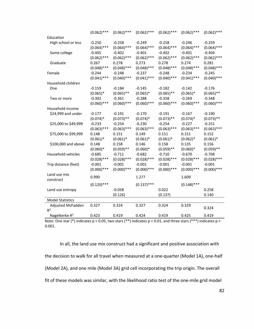
82

(0.062)*** (0.062)*** (0.062)*** (0.062)*** (0.062)*** (0.062)*** Education High school or less -0.250 -0.258 -0.249 -0.258 -0.246 -0.259 (0.064)*** (0.064)*** (0.064)*** (0.064)*** (0.064)*** (0.064)*** Some college -0.405 -0.402 -0.401 -0.402 -0.401 -0.404 (0.062)*** (0.062)*** (0.062)*** (0.062)*** (0.062)*** (0.062)*** Graduate 0.267 0.278 0.273 0.278 0.274 0.281 (0.048)*** (0.048)*** (0.048)*** (0.048)*** (0.048)*** (0.048)*** Female -0.244 -0.248 -0.237 -0.248 -0.234 -0.245 (0.041)*** (0.040)*** (0.041)*** (0.040)*** (0.041)*** (0.040)*** Household children One -0.159 -0.184 -0.145 -0.182 -0.142 -0.176 (0.065)* (0.065)** (0.065)* (0.065)** (0.065)* (0.065)** Two or more -0.302 -0.361 -0.288 -0.358 -0.269 -0.348 (0.060)*** (0.060)*** (0.060)*** (0.060)*** (0.060)*** (0.060)*** Household income $24,999 and under -0.177 -0.191 -0.170 -0.191 -0.167 -0.190 (0.074)* (0.073)** (0.074)* (0.073)** (0.074)* (0.073)** $25,000 to $49,999 -0.233 -0.254 -0.230 -0.254 -0.227 -0.251 (0.063)*** (0.063)*** (0.063)*** (0.063)*** (0.063)*** (0.063)*** $75,000 to $99,999 0.148 0.151 0.149 0.151 0.151 0.152 (0.061)* (0.061)* (0.061)* (0.061)* (0.062)* (0.061)* $100,000 and above 0.148 0.158 0.146 0.158 0.135 0.156 (0.060)* (0.059)** (0.060)* (0.059)** (0.060)* (0.059)** Household vehicles -0.685 -0.711 -0.682 -0.710 -0.670 -0.708 (0.028)*** (0.028)*** (0.028)*** (0.028)*** (0.028)*** (0.028)*** Trip distance (feet) -0.001 -0.001 -0.001 -0.001 -0.001 -0.001 (0.000)*** (0.000)*** (0.000)*** (0.000)*** (0.000)*** (0.000)*** Land use mix construct

0.990 1.277 1.609

(0.120)*** (0.137)*** (0.148)*** Land use entropy -0.058 0.022 0.258 (0.126) (0.137) 0.140

Model Statistics

Adjusted McFadden R2

0.327 0.324 0.327 0.324 0.329 0.324

Nagelkerke R2 0.423 0.419 0.424 0.419 0.425 0.419

Note: One star (*) indicates p < 0.05, two stars (**) indicates p < 0.01, and three stars (***) indicates p < 0.001.

In all, the land use mix construct had a significant and positive association with

the decision to walk for all travel when measured at a one-quarter (Model 1A), one-half

(Model 2A), and one mile (Model 3A) grid cell incorporating the trip origin. The overall

fit of these models was similar, with the likelihood ratio test of the one-mile grid model

83

(χ^2(1) = 125.79, p<0.001) revealing the greatest improvement in goodness of fit over

the reduced model. An increase in land use mix measured at this one-mile scale was

positively associated with pedestrian travel, with a one standard deviation increase in

the mean land use mix score translating to a fivefold increase in the odds of walking (B =

1.609, SE = 0.148, p<0.001, odds ratio [OR] = 5.00, confidence interval [CI] = 3.75 – 6.69).

Although the magnitude of this link declined as the scale of measurement decreased, a

one standard deviation increase in land use mixing within a quarter-mile of the origin

resulted in a person being over two times as likely to walk (B = 0.990, SE = 0.120,

p<0.001, OR = 2.69, CI = 2.13 – 3.40). Accordingly, travelers originating from a landscape

with a heightened complexity in the composition and configuration of local land uses

are more likely to walk than individuals traveling from a less mixed landscape.

In contrast, while past studies have concluded that an increase in the evenness

of land use types has a strong positive connection to pedestrian activity (see Brownson,

et al., 2009), study findings show otherwise. The addition of a land use entropy

measure, operationalized at any of three scales incorporating the trip origin, to the

reduced specification produced no significant contribution to the modeled decision to

walk. In fact, land use diversity measured at the most localized neighborhood scale

(Model 1B) had a counterintuitive, but non-significant, association with the likelihood to

walk. Increasing the geographic extent corrected this theoretical mismatch; however, an

increased land use entropy at a one-mile landscape (Model 3B) had only a marginally

significant relationship with an individual’s likelihood to walk (B = 0.258, SE = 0.140, p =

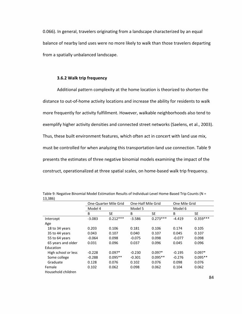
84

0.066). In general, travelers originating from a landscape characterized by an equal

balance of nearby land uses were no more likely to walk than those travelers departing

from a spatially unbalanced landscape.

3.6.2 Walk trip frequency

Additional pattern complexity at the home location is theorized to shorten the

distance to out-of-home activity locations and increase the ability for residents to walk

more frequently for activity fulfillment. However, walkable neighborhoods also tend to

exemplify higher activity densities and connected street networks (Saelens, et al., 2003).

Thus, these built environment features, which often act in concert with land use mix,

must be controlled for when analyzing this transportation-land use connection. Table 9

presents the estimates of three negative binomial models examining the impact of the

construct, operationalized at three spatial scales, on home-based walk trip frequency.

Table 9: Negative Binomial Model Estimation Results of Individual-Level Home-Based Trip Counts (N = 13,386)

One-Quarter Mile Grid One-Half Mile Grid One Mile Grid

Model 4 Model 5 Model 6

B SE B SE B SE

Intercept -3.083 0.212*** -3.586 0.273*** -4.419 0.359*** Age 18 to 34 years 0.203 0.106 0.181 0.106 0.174 0.105 35 to 44 years 0.043 0.107 0.040 0.107 0.045 0.107 55 to 64 years -0.064 0.098 -0.075 0.098 -0.077 0.098 65 years and older 0.031 0.096 0.037 0.096 0.045 0.096 Education High school or less -0.228 0.097* -0.230 0.097* -0.195 0.097* Some college -0.288 0.095** -0.301 0.095** -0.276 0.095** Graduate 0.128 0.076 0.102 0.076 0.098 0.076 Female 0.102 0.062 0.098 0.062 0.104 0.062 Household children

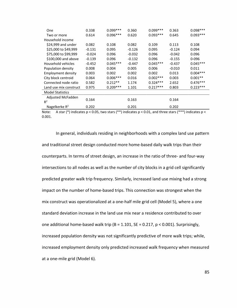
85

One 0.338 0.099*** 0.360 0.099*** 0.363 0.098*** Two or more 0.614 0.096*** 0.620 0.093*** 0.645 0.093*** Household income $24,999 and under 0.082 0.108 0.082 0.109 0.113 0.108 $25,000 to $49,999 -0.131 0.095 -0.126 0.095 -0.124 0.094 $75,000 to $99,999 -0.024 0.096 -0.032 0.096 -0.042 0.096 $100,000 and above -0.139 0.096 -0.132 0.096 -0.155 0-096 Household vehicles -0.452 0.045*** -0.447 0.045*** -0.437 0.045*** Population density 0.008 0.004 0.005 0.006 -0.010 0.011 Employment density 0.003 0.002 0.002 0.002 0.013 0.004*** City block centroid 0.064 0.006*** 0.016 0.002*** 0.003 0.001** Connected node ratio 0.582 0.212** 1.174 0.324*** 2.652 0.476*** Land use mix construct 0.975 0.209*** 1.101 0.217*** 0.803 0.223***

Model Statistics

Adjusted McFadden R2 0.164 0.163 0.164

Nagelkerke R2 0.202 0.201 0.202

Note: A star (*) indicates p < 0.05, two stars (**) indicates p < 0.01, and three stars (***) indicates p < 0.001.

In general, individuals residing in neighborhoods with a complex land use pattern

and traditional street design conducted more home-based daily walk trips than their

counterparts. In terms of street design, an increase in the ratio of three- and four-way

intersections to all nodes as well as the number of city blocks in a grid cell significantly

predicted greater walk trip frequency. Similarly, increased land use mixing had a strong

impact on the number of home-based trips. This connection was strongest when the

mix construct was operationalized at a one-half mile grid cell (Model 5), where a one

standard deviation increase in the land use mix near a residence contributed to over

one additional home-based walk trip (B = 1.101, SE = 0.217, p < 0.001). Surprisingly,

increased population density was not significantly predictive of more walk trips; while,

increased employment density only predicted increased walk frequency when measured

at a one-mile grid (Model 6).

86

3.7 Limitations

Future extensions of this study should address its limitations. A full structural

equation framework would allow retention of the latent construct in the measurement

model and offer a more complete behavioral depiction of the transportation-land use

connection. Adoption of a CFA measurement strategy aided the creation of a

multifaceted land use mix construct with composition and configuration indicators;

however, the value of a single measure of each pattern aspect warrants further

investigation. The specification of separate configuration and composition measures,

while likely to be interrelated, may produce different statistical associations with the

tested behaviors since one aspect may be a stronger determinant of walking than the

other. Also, while the ARC composition measure is a novel way to provide theoretical

support for quantifying land use balance, other possibilities for relating functional

complementarity to travel behavior remain.

Moreover, the inherent relationship between spatial scale choice and built

environment measurement merits closer attention. In this study, each indicator was

operationalized at three grid cell sizes to offer insight into the sensitivity of scale choice

on land use mix measurement. CFA results support construct stability across multiple

spatial scales; yet, further work is needed to examine the impact of capturing land use

mix with areal or network buffers. Finally, the validity of this measure should be studied

in other contexts to identify its transferability to settings with weaker growth

management policies.

87

3.8 Conclusions

Planning research has long pointed to the transportation benefits of land use

mixing; however, this link has been commonly analyzed using insufficient measures. This

study introduces a land use mix measurement of the composition and configuration of

local land use types and demonstrates the construct’s link to pedestrian travel. Planning

literature has portrayed land use mix as an environmental phenomenon describing the

access to diverse activity locations, intensity of these opportunities, and spatial

integration of those land use types affiliated with these activities. Accordingly, the

findings suggest that complexity in this spatial construct is best expressed as a set of

indicators portraying these multiple aspects.

Study contributions are both conceptual and methodological. Presenting a mix

indicator based on the activity-related complementarity of land use types may help

redirect how ideal compositional balance is measured. By evaluating the area-based

balance of all land use types, entropy indices offer limited guidance for directing smart

growth policies. This application of a land use mix indicator based on the observed

compatibility of activity-related travel may better direct policies intended to produce

greater transportation efficiencies by closely locating synergistic land uses. The

introduced construct also reflects the spatial heterogeneity of land use types by

accounting for the overall maximum patch size and intermixing of dissimilar landscape

patches. By not explicitly measuring configuration, commonly adopted pattern

measures (e.g., entropy index) are insensitive to any spatial integration. Attention to

88

configuration, while nascent, may provide planners further understanding into the

development patterns that best achieve land use efficiencies. The use of a CFA modeling

framework enabled the construction of an activity-related mix measure that accounts

for both composition and configuration.

If adopted by planning researchers and practitioners, a refined measure of land

use mix incorporating these unique theoretical components of landscape pattern may

also reveal richer insight into the influence of local land use mixing on pedestrian trip-

making. In this study, the proposed latent construct had a stronger association with

walk mode choice than the atheoretical entropy index. Additionally, the construct was

significantly linked to the frequency of home-based walk trips when tested in a

behavioral model controlling for other features of the traveler’s home built

environment. Of particular interest, population and employment density had no

significant impact at the more localized scales when controlling for the mix construct as

a co-determinant of walking. Such findings may shift future land development

discussions away from contentious debates on neighborhood densification and toward a

dialogue of how development may be spatially configured to promote local accessibility

and physical activity. Overall, the authors believe this work provides valuable insight

into the measurement of land use mix as a multifaceted construct with clear positive

connections to pedestrian travel.

89

Chapter 4: A Pathway Linking Smart Growth Neighborhood to Home-Based Pedestrian

Travel

4.1 Introduction

Urban planners and transportation experts have pointed to smart growth

development as a response to a pressing need for improving transportation-related

physical activity levels and environmental quality (Saelens, et al., 2003). The prevailing

rationale is that land development patterns and urban design, which are impacted by

transportation policies and investments, are inextricably linked to travel behaviors and

outcomes (Handy, 2005). This connection underscores a desirability for smart growth

communities, which bring residents closer to out-of-home activity destinations and

improve their feasibility of reaching those locations by walking (Handy, et al., 2002).

Accordingly, smart growth and other integrated transportation-land use investment

strategies must continue to be pursued in order to develop activity friendly, walkable

environments that support increased physical activity (Frank & Kavage, 2009).

Smart growth neighborhoods exhibit compact development patterns with higher

densities, land use diversity, and a pedestrian-friendly design aimed at minimizing

automobile use for short trips (Downs, 2005). The formation of these sustainable

communities was a policy goal in the 2014-2018 strategic plan of the US Environmental

Protection Agency and previously envisioned within a suite of livability principles guiding

its 2009 Interagency Partnership for Sustainable Communities with the US Departments

90

of Transportation and Housing and Urban Development. However, questions regarding

the identification of a set of built environment indicators and creation of commonly

accepted standards for what constitutes a walkable, smart growth neighborhood largely

continue to be unanswered (Clifton, et al., 2007). An unlikely circumstance that exists

despite a popularity in transportation-land use research rising from the potential to

moderate travel behaviors and patterns by altering the physical environment in

accordance with smart growth policy (Ewing & Cervero, 2010).

This policy discussion remains because past active travel behavior studies have

adopted imperfect measures to reflect the interrelated dimensions characterizing the

built environment (Handy, et al., 2002). Although recent studies have used more

sophisticated statistical methods to estimate the effects of more environmental factors

(Ewing & Cervero, 2010), these studies tend to depict the built environment as a series

of isolated measures rather than a comprehensive collection of synergistic indicators

reflecting its multidimensionality. Factor analysis has gained approval as one method to

derive generalized dimensions of neighborhood character from isolated measures that

may display conceptual or empirical redundancy (Song & Knaap, 2007). The use of this

method to recognize the built environment as a multidimensional concept can offer

insight into measurement selection and the cumulative impact of altering interrelated

land development pattern, urban design, and transportation system factors comprising

this higher-order construct on travel behavior.

91

The impact of residing in a smart growth neighborhood on walking may also not

be fully realized because the indirect effects of the various explanatory factors

influencing one another and travel behavior have been inadequately examined (Van

Acker, et al., 2007). A host of individual, societal, and contextual factors is hypothesized

to predict walking for both transportation and recreational purposes (Pikora, et al.,

2003). However, by not accounting for the indirect effects of these characteristics,

which may diminish or confound the total effect of the built environment on pedestrian

travel, studies may offer an incomplete picture of this transportation-land use

connection. In all, the precise nature of residing in a smart growth community on travel

behavior cannot be entirely understood without a conceptual and methodological

framework specifying the many pathways to and determinants of travel (Bagley &

Mokhtarian, 2002).

The objectives of this study are twofold. First, this study introduces a

multidimensional concept of the physical environment reflecting several heralded

tenets of smart growth policy. Second, this paper proposes a framework linking this

second-order environmental construct and sociodemographic aspects to pedestrian

travel and tests these complex interactions using structural equation modeling (SEM).

By doing so, this paper offers a novel and robust measure of what constitutes a smart

growth neighborhood and extended understanding of how this multidimensional

concept influences household-level pedestrian travel.

92

4.2 Literature Review

Of the existing studies linking a built environment construct to travel behavior

using SEM techniques, the measurement of identified indicators has been either

objective, perceived, or some combination (Ma, et al., 2014). Further, once a construct

has been confirmed, a number of travel outcomes and behaviors have been explored by

using pathways illustrated in a variety of proposed conceptual frameworks. The

following subsections review the SEM evidence base linking built environment

constructs to travel and recommend a conceptual framework to guide this study’s

analysis of household-level pedestrian travel.

4.2.1 Structural equation models of the transportation-land use connection

While most transportation-land use studies focus on objective built environment

measurement, several SEM applications have identified built environment constructs

based on individual perceptions. These studies have explored themes of neighborhood

accessibility (Cao, et al., 2007, Cao, 2016), arrangement and aesthetic (Aditjandra, et al.,

2012; Aditjandra & Mulley, 2016; Banerjee & Hine, 2016) and sense of place (Deutsch,

et al., 2013) to recognize their influence on automobile ownership and travel mode

choice. Other studies have identified residential environments as single constructs

containing both perceived and objective indicators (Bagley & Mokhtarian, 2002) or as

distinct constructs reflecting an individual’s objective and perceived residential

environment (Ma, et al., 2014).

93

In a San Francisco Bay Area study, Bagley and Mokhtarian (2002) identified

separate constructs for traditional and suburban environments to estimate the impact

of neighborhood types, lifestyles, and attitudes on miles traveled via automobile, public

transit, and active transport. The objectively measured indicators of the traditional

environment included population density, grid-like street design, and speed limit of the

road (Bagley, et al., 2002). In a Portland-based study examining the effect of objective

and perceived environments on monthly cycling rates, Ma et al. (2014) described an

objective environment with built environment indicators including the number of

business establishments, percent of connected streets, and miles of bike infrastructure

near an individual’s home. Consequently, the construct better represented an objective

bicycling environment rather than a residential environment; underscoring the

importance in selecting measurement variables that reflect a residence’s overall built

environment (de Abreau e Silva, et al., 2012b).

In the European context, several studies have examined the impact of land

development patterns on travel behavior. Van Acker et al. (2007) examined this path

with a land use factor reflecting the distance to public transit and two categorical

indicators of the residential environment in Flanders. Their results indicated land use

had a positive direct effect on a travel behavior construct reflecting the total distance,

duration, and number of trips originating from the home location. A second study by

Van Acker and Witlox (2010) examined the mediating effect of auto ownership on the

path connecting the built environment to automobile use. While this latter study had

94

additional variables related to land development and patterns, the SEM application does

not describe the residential environment as a multidimensional construct. Eboli et al.

(2012) explored the land use-travel behavior link with latent factors for each, in

southern Italy. Land use was indicated by only two objective measures: housing unit

surface area and residential environment.

Using a more comprehensive set of built environment indicators, a series of

papers addressed the impact of land patterns on short- and long-term travel behavior

decisions in Lisbon (de Abreu e Silva, et al., 2006), Seattle (de Abreu e Silva & Goulias,

2009), Montreal (de Abreu e Silva, et al., 2012b), and Los Angeles (de Abreu e Silva, et

al., 2012a). In the first paper, a traditional urban land use factor largely driven by

population density and public transit supply at the residence predicted an increase in

distance traveled and trip frequency for nonmotorized travel modes. The authors then

identified a residential environment construct with Montreal data reflective of land use

entropy and automobile accessibility as well as a pair of home- and job-based constructs

described as a central, denser, and accessible area. In the American context, this

multidimensional construct describing a dense and centrally-located residential

environment indicated by population, building, and intersection density as well as

distance to the central business district was identified in Seattle. Finally, the Los Angeles

study examined the link to trip scheduling from a residential land use construct with

indicators representing the activity participation opportunity.

95

Overall, only a handful of studies have exclusively represented the built

environment as a set of objectively measured indicators describing a multidimensional

latent construct. In contrary to perceived environmental measures, a construct

composed of objective measurements is not subjected to reporting bias that may inflate

the effect of residing in a smart growth community on pedestrian travel (Aditjandra &

Mulley, 2016). Further, those SEM studies detailing a construct with objective indicators

have tended to examine its influence on auto-related outcomes rather than pedestrian

travel patterns and behaviors. While smart growth communities provide an alternative

to auto-oriented neighborhoods, policies related to improving community livability via

increased transportation-related physical activity levels are provided limited insight by

past studies focused solely on auto travel (Handy, 2005).

4.2.2 Conceptual framework

A framework describing the built environment and transportation connection is

provided in Figure 4. The built environment is comprised of land development patterns,

urban design, and transportation system features (Frank & Engelke, 2001; Handy, 2005).

Land development patterns describe the land use mix (distance-based accessibility,

intensity, and pattern) as well as the intensity or density of features in a defined spatial

extent, while urban design features detail the arrangement and aesthetics of the built

environment (Handy, et al., 2002). The transportation system refers to both the physical

infrastructure available to an individual and the performance or quality of any provision.

96

Figure 4: Proposed Conceptual Framework Linking the Built Environment to Travel Behaviors and Patterns

In the proposed framework, the built environment features are determined by

sociodemographic attributes of an individual, household, and his/her neighborhood

(Van Acker, et al., 2007), which in turn have a direct effect on travel outcomes such as

walk mode choice (Saelens, et al., 2003). Sociodemographic and economic features may

include, but are not limited to, a person’s age, income, education, gender, or access to

private transport options (Ma, et al., 2014) in addition to the sociodemographic and

economic composition of his/her household and neighbors. Contextual factors such as

government policy and the natural environment also impact travel behaviors and

patterns, but are considered to be external to the built environment and

sociodemographic influences (Panter, et al., 2008).

4.3 Data and Methods

This section describes a methodology for adopting this framework to (a) provide

a multidimensional construct reflecting three distinct built environment facets and (b)

97

estimate the impact of a second-order construct representing a smart growth

neighborhood on household-level, home-based pedestrian travel.

4.3.1 Study area and sample

This study examined the travel behaviors of residents in the three Oregon

counties spanning the Portland metro region: Multnomah, Clackamas, and Washington.

The decision to broaden the study area beyond the region’s state mandated growth

boundary enabled measurement of the transportation-land use connection in

neighborhoods both impacted and not by the enactment of regional growth controls.

Respondents of the Oregon Household Activity Survey (OHAS), a statewide

transportation survey detailing weekday activity and travel patterns of randomly

sampled households, completed a one-day travel diary for themselves and each

member of their household. Survey participants also reported information about their

activity locations, trip purposes, trip distances, and travel mode choices as well as

sociodemographic and economic characteristics of each household member. Table 10

summarizes the descriptive statistics for the study sample of 4,416 households surveyed

in the three-county study area during 2011.

Table 10: Household-Level Descriptive Statistics of Study Sample

Indicator Name n % Mean St. Dev. Min Max

Sociodemographic and Economic Characteristics

Number of children under 6 years --- --- 0.14 0.45 0.00 4.00 Number of children 6 years or older --- --- 0.32 0.71 0.00 5.00 Number of adults --- --- 1.95 0.79 1.00 7.00

98

Non-related household 129 0.03 --- --- 0.00 1.00 Annual income: Under $25,000 505 0.12 --- --- 0.00 1.00 Annual income: $25,000 to $49,999 823 0.20 --- --- 0.00 1.00 Annual income: $50,000 to $99,999 1,675 0.41 --- --- 0.00 1.00 Annual income: $100,000 or more 1,080 0.26 --- --- 0.00 1.00 Household workers: 0 864 0.20 --- --- 0.00 1.00 Household workers: 1 1,800 0.41 --- --- 0.00 1.00 Household workers: 2 1,557 0.35 --- --- 0.00 1.00 Household workers: 3 or more 195 0.04 --- --- 0.00 1.00 Oldest adult: Under 30 years 127 0.03 --- --- 0.00 1.00 Oldest adult: 30 to 44 years 892 0.21 --- --- 0.00 1.00 Oldest adult: 45 to 64 years 2,198 0.51 --- --- 0.00 1.00 Oldest adult: 65 years or more 1,131 0.26 --- --- 0.00 1.00 Education: High school diploma or less 358 0.08 --- --- 0.00 1.00 Education: Associate’s degree or credits 982 0.22 --- --- 0.00 1.00 Education: Bachelor’s degree 1,434 0.33 --- --- 0.00 1.00 Education: Graduate degree 1,635 0.37 --- --- 0.00 1.00

Transportation Characteristics

Vehicles per licensed driver --- --- 1.05 0.56 0.00 8.00 Transit passes per adult --- --- 0.16 0.31 0.00 1.00 Bikes per person 6 years or older --- --- 0.55 0.71 0.00 13.00

Home-based Travel Behaviors and Patterns

Average trip distance (miles) --- --- 4.33 3.87 0.01 29.63 Walked for transportation purposes 541 0.12 --- --- 0.00 1.00 Walked for discretionary purposes 232 0.05 --- --- 0.00 1.00

Notes: Dashes (---) indicate frequencies (n) were not provided for continuous measures. A star (*) indicates a binary measure of the household-level decision to make 0 vs. ≥1 walk trips.

4.3.2 Built environment measurement

A one-mile areal buffer centered on the home location, which approximates the

distance that an individual may travel on a 20-minute walk originating from his/her

home, was selected to delineate the residential neighborhood of sampled OHAS

respondents. To understand the multidimensionality of the built environment measured

at the home location and its connection to household-level pedestrian travel, an

extensive set of 62 built environment indicators related to land development patterns,

urban design features, and transportation infrastructure was assessed in both urban and

non-urban contexts. Table 11 details this list of built environment measures from

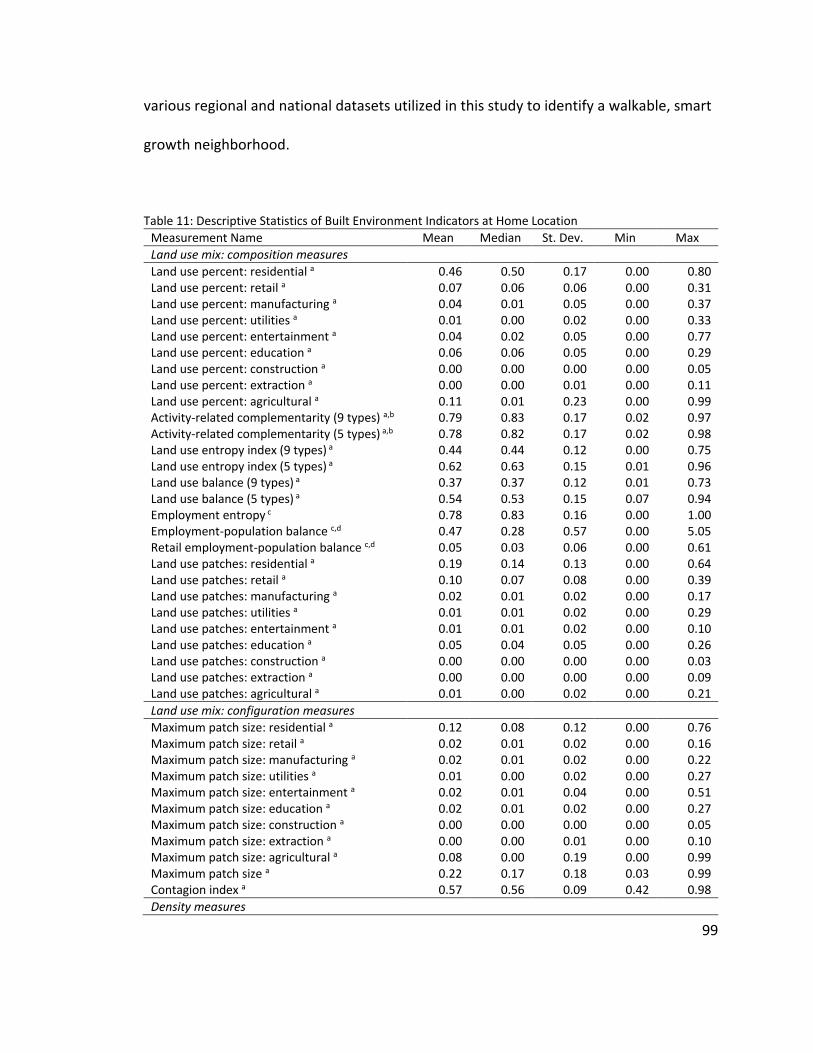
99

various regional and national datasets utilized in this study to identify a walkable, smart

growth neighborhood.

Table 11: Descriptive Statistics of Built Environment Indicators at Home Location

Measurement Name Mean Median St. Dev. Min Max

Land use mix: composition measures

Land use percent: residential a 0.46 0.50 0.17 0.00 0.80 Land use percent: retail a 0.07 0.06 0.06 0.00 0.31 Land use percent: manufacturing a 0.04 0.01 0.05 0.00 0.37 Land use percent: utilities a 0.01 0.00 0.02 0.00 0.33 Land use percent: entertainment a 0.04 0.02 0.05 0.00 0.77 Land use percent: education a 0.06 0.06 0.05 0.00 0.29 Land use percent: construction a 0.00 0.00 0.00 0.00 0.05 Land use percent: extraction a 0.00 0.00 0.01 0.00 0.11 Land use percent: agricultural a 0.11 0.01 0.23 0.00 0.99 Activity-related complementarity (9 types) a,b 0.79 0.83 0.17 0.02 0.97 Activity-related complementarity (5 types) a,b 0.78 0.82 0.17 0.02 0.98 Land use entropy index (9 types) a 0.44 0.44 0.12 0.00 0.75 Land use entropy index (5 types) a 0.62 0.63 0.15 0.01 0.96 Land use balance (9 types) a 0.37 0.37 0.12 0.01 0.73 Land use balance (5 types) a 0.54 0.53 0.15 0.07 0.94 Employment entropy c 0.78 0.83 0.16 0.00 1.00 Employment-population balance c,d 0.47 0.28 0.57 0.00 5.05 Retail employment-population balance c,d 0.05 0.03 0.06 0.00 0.61 Land use patches: residential a 0.19 0.14 0.13 0.00 0.64 Land use patches: retail a 0.10 0.07 0.08 0.00 0.39 Land use patches: manufacturing a 0.02 0.01 0.02 0.00 0.17 Land use patches: utilities a 0.01 0.01 0.02 0.00 0.29 Land use patches: entertainment a 0.01 0.01 0.02 0.00 0.10 Land use patches: education a 0.05 0.04 0.05 0.00 0.26 Land use patches: construction a 0.00 0.00 0.00 0.00 0.03 Land use patches: extraction a 0.00 0.00 0.00 0.00 0.09 Land use patches: agricultural a 0.01 0.00 0.02 0.00 0.21

Land use mix: configuration measures

Maximum patch size: residential a 0.12 0.08 0.12 0.00 0.76 Maximum patch size: retail a 0.02 0.01 0.02 0.00 0.16 Maximum patch size: manufacturing a 0.02 0.01 0.02 0.00 0.22 Maximum patch size: utilities a 0.01 0.00 0.02 0.00 0.27 Maximum patch size: entertainment a 0.02 0.01 0.04 0.00 0.51 Maximum patch size: education a 0.02 0.01 0.02 0.00 0.27 Maximum patch size: construction a 0.00 0.00 0.00 0.00 0.05 Maximum patch size: extraction a 0.00 0.00 0.01 0.00 0.10 Maximum patch size: agricultural a 0.08 0.00 0.19 0.00 0.99 Maximum patch size a 0.22 0.17 0.18 0.03 0.99 Contagion index a 0.57 0.56 0.09 0.42 0.98

Density measures

100

Population d 15,075 14,371 7,655 48.26 38,944 Housing units d 6,783 6,189 4,298 8.32 27,237 Employment c 7,881 4,188 14,230 0.00 115,360 Office jobs c 1,468 355 4,546 0.00 39,168 Retail jobs c 808 473 1,070 0.00 6,622 Industrial jobs c 1,354 597 1,901 0.00 12,487 Service jobs c 3,198 1,599 5,433 0.00 40,272 Entertainment jobs c 922 434 1,907 0.00 14,735 Total activity (population and employment) c,d 22,956 19,998 19,037 56.36 143,129

Urban design and transportation system measures

Census blocks d 300 214 224 1.00 1,085 Street blocks e 243 146 216 0.00 918 Connected node ratio e 0.74 0.71 0.12 0.13 1.00 Alpha index e 0.23 0.19 0.12 -1.00 3.00 Beta index e 1.46 1.38 0.21 1.06 2.02 Gamma index e 0.49 0.46 0.08 0.37 3.00 Intersections e 432 391 228 1.00 1,065 Cul-de-sacs e 126 117 68.59 0.00 330 Primary roads (miles) e 1.37 0.00 1.97 0.00 9.17 Secondary roads (miles) e 1.59 1.65 1.47 0.00 8.05 Local roads (miles) e 53.00 51.18 21.37 0.67 101 Percent of primary roads e 0.02 0.00 0.03 0.00 0.31 Percent of secondary roads e 0.03 0.02 0.04 0.00 0.75 Percent of local roads e 0.93 0.94 0.06 0.25 1.00 Sidewalk coverage e 0.45 0.46 0.27 0.00 0.98

Note: Land use type taxonomy adopted from American Planning Association’s Land-Based Classification Standards. Superscripts (n) indicate the measurement’s data source: (a) 2011 Regional Land Information System, (b) 2011 Oregon Household Activity Survey, (c) 2014 Longitudinal Employer-Household Dynamic, (d) 2010 US Census, and (e) 2010 US Census Topologically Integrated Geographic Encoding and Referencing.

Land use mix embodies a subset of land development pattern measures

describing both the composition and configuration of land use types in a landscape

(Gehrke & Clifton, 2016). Portland Metro’s Regional Land Information System provided

parcel-level data to calculate composition measures characterizing the percent of land

area or patches of each land use type in a landscape and configuration measures

explicitly accounting for the spatial arrangement, shape, and dissimilarity of the

landscape patches (Li & Reynolds, 1994; Turner, 2005). Other measures considered the

proportion of all or a reduced set of five (residential, retail, entertainment, education,

101

and other) land use types, including the land use entropy index (Cervero, 1989) and

measures of land use balance (Bhat & Gossen, 2004) and activity-related

complementarity (ARC). The ARC measure represents the localized balance of land use

types based on a derived demand for travel rather than their spatial equilibrium.

𝐴𝑅𝐶 = 1 − ∑ [𝑃𝑖 ∗|𝑃𝑖−𝐹𝑖|

1−𝐹𝑖]𝑛

𝑖=1 (3)

In Equation 3, 𝑛 is the number of land use types, 𝑃𝑖 is the proportion of area

dedicated to land use type 𝑖, and 𝐹𝑖 is an activity factor associated with each land use

type in a neighborhood. These activity factors measure the percentage of trip ends

terminating at one of nine land use categories: 𝐹𝑅𝐸𝑆 = 0.42, 𝐹𝑅𝐸𝑇 = 0.32, 𝐹𝐼𝑁𝐷 = 0.03,

𝐹𝑈𝑇𝐼 = 0.01, 𝐹𝐸𝑁𝑇 = 0.02, 𝐹𝐸𝐷𝑈 = 0.16, 𝐹𝐶𝑂𝑁 = 0.01, 𝐹𝐸𝑋𝑇 = 0.01, and 𝐹𝐴𝐺𝑅 = 0.04.

For instance, in the study sample, 42-percent of all trips concluded at an activity location

within a residential land use type. In the end, a score of zero indicates a neighborhood

dominated by a single land use type; whereas, a score of one indicates a neighborhood

where the spatial allocation of all land use types perfectly matches the observed

attraction for activities.

The remaining composition measures in Table 11 describe the jobs-housing

balance of a residential environment and its employment entropy, as measured by the

diversity of office, retail, industrial, service, and entertainment jobs. In turn, the

configuration of a landscape was measured by either computing the maximum patch

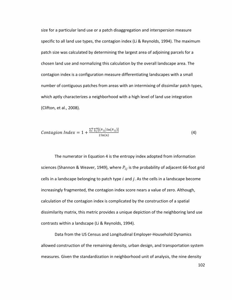
102

size for a particular land use or a patch disaggregation and interspersion measure

specific to all land use types, the contagion index (Li & Reynolds, 1994). The maximum

patch size was calculated by determining the largest area of adjoining parcels for a

chosen land use and normalizing this calculation by the overall landscape area. The

contagion index is a configuration measure differentiating landscapes with a small

number of contiguous patches from areas with an intermixing of dissimilar patch types,

which aptly characterizes a neighborhood with a high level of land use integration

(Clifton, et al., 2008).

𝐶𝑜𝑛𝑡𝑎𝑔𝑖𝑜𝑛 𝐼𝑛𝑑𝑒𝑥 = 1 +∑ ∑ [(𝑃𝑖𝑗) ln(𝑃𝑖𝑗)]𝑛

𝑗𝑛𝑖

2 ln(𝑛) (4)

The numerator in Equation 4 is the entropy index adopted from information

sciences (Shannon & Weaver, 1949), where 𝑃𝑖𝑗 is the probability of adjacent 66-foot grid

cells in a landscape belonging to patch type 𝑖 and 𝑗. As the cells in a landscape become

increasingly fragmented, the contagion index score nears a value of zero. Although,

calculation of the contagion index is complicated by the construction of a spatial

dissimilarity matrix, this metric provides a unique depiction of the neighboring land use

contrasts within a landscape (Li & Reynolds, 1994).

Data from the US Census and Longitudinal Employer-Household Dynamics

allowed construction of the remaining density, urban design, and transportation system

measures. Given the standardization in neighborhood unit of analysis, the nine density

103

measures are simply continuous variables denoting the number of persons, housing

units, or jobs surrounding a home location. Urban design features in Table 11 include

common transportation planning measures such as the number of blocks, intersections,

and cul-de-sacs as well as three network connectivity indices (Song, et al., 2013). Finally,

the seven transportation infrastructure measures describe the total length and percent

of primary, secondary, and local roads in addition to the sidewalk coverage along these

facilities.

A distillation process followed to reduce these built environment measures to a

parsimonious set of indicators. The first step was to examine a correlation matrix and

eliminate measures that were highly associated and pointed toward concept

redundancy. A subsequent step was to perform an exploratory factor analysis (EFA) to

identify an exclusive yet comprehensive collection of interrelated measures that reflect

the land development pattern, urban design, and transportation system found within a

residential environment. The EFA technique helped generate a theoretic understanding

of the internal structure of how observed built environment measures may improve the

construct measurement of a smart growth neighborhood. The assumption being that

factors shaped by this exploratory technique may also be useful as operational

descriptions of the three built environment dimensions.

The EFA was performed in sequential steps centered on three decisions related

to selection of a factor model approach, extraction scheme, and rotation method (Ford,

et al., 1986). Principal axis factoring was used since this method has generally

104

outperformed other methods in recovering factors with low loadings, providing

solutions with stable loadings, and isolating correlated factors (de Winter & Dodou,

2012). The inspection of eigenvalues associated with each resulting factor and their

scree plot display guided the factor extraction (Hayton, et al., 2004). Finally, a promax

rotation, which allows for correlation between the extracted factors, was chosen as a

rotation method leading to the final three-factor model described in Table 12.

Table 12: Exploratory Factor Analysis of Built Environment Characteristics

Built Environment Characteristics

Factor 1: Land use dominance

Factor 2: Employment concentration

Factor 3: Pedestrian-oriented design

Land use activity-related complementarity (9 types) -0.96 0.00 -0.01 Employment entropy -0.52 0.05 0.05 Employment-population balance -0.03 0.91 -0.07 Land use patches: retail 0.10 0.15 0.92 Maximum patch size: agricultural 0.90 0.04 0.03 Maximum patch size 0.97 0.12 0.07 Contagion index 0.86 -0.19 -0.01 Office jobs 0.07 0.93 -0.02 Retail jobs -0.06 0.71 0.20 Connected node ratio 0.04 -0.06 0.95 Sidewalk coverage -0.19 -0.16 0.69

Eigenvalue 5.51 2.20 1.23 Percent of variance explained 50.09 19.96 11.22

Notes: Factor loadings > 0.4 are in bold.

The results of this initial diagnostic step produced three built environment

factors based on a set of smart growth indicators. Factor 1 comprises two composition

and three configuration indicators of land use mix. Taken together, this land use

dominance factor reflects a residential environment with a limited complementarity in

land use types, imbalance of employment opportunities, and high patch aggregation or

105

isolation, independent of the land uses in a neighborhood. Three land development

pattern indicators were also found to strongly reflect Factor 2. The ratio of total

employment-to-persons is a commonly adopted proxy measure for land use mixing;

whereas, the number of office- and retail-related jobs within a one-mile radius around a

residence also contributed to this employment concentration factor. The final factor

was explained by two urban design and transportation system indicators, connected

node ratio and sidewalk coverage, as well as a third indicator measuring the number of

retail land use patches. Overall, the adoption of an EFA framework before estimating

the structural model permitted an empirically-driven process for understanding the

interrelationships between a collection of objective indicators, which may be supported

by a priori theory to reflect potential underlying latent constructs (Brown, 2006).

4.3.3 Structural equation modeling

Application of an SEM method with latent constructs is a firmly established analytic

strategy in which a set of specified equations containing measurement models for

exogenous and endogenous variables are concurrently estimated with a structural

model estimating the associations or pathways between (Golob, 2003). Using a two-step

approach, the measurement models positing the relationship of observed variables to a

latent construct were estimated by confirmatory factor analysis (CFA) before an

assessment of a structural model with path assignments (Anderson & Gerbing, 1988).

The application of this strategy offers several advantages over conventional multivariate

106

regression methods, including the ability to: (a) develop latent constructs with multiple

indicators, (b) correct for measurement error in the observed variables reflecting any

latent construct, and (c) simultaneously test for both direct and indirect effects as well

as any bidirectional relationships that exist between multiple variables across different

paths (Golob, 2003; Van Acker, et al., 2007; Aditjandra, et al., 2012; de Abreu e Silva, et

al., 2012a). However, while this latter point constitutes a conceptual improvement over

a single-equation approach, using cross-sectional data in any SEM application still does

not infer the condition of time precedence needed to establish a causal relationship

(Cao, et al., 2007).

The pathways of greatest interest to this study are the direct and indirect effects

of the latent construct reflecting a smart growth neighborhood on the household-level

decision to conduct a walk trip for transportation (mandatory or subsistence) or

discretionary trip purposes. Although, the use of SEM also allows for the simultaneous

testing of the direct and total effects of several household-level measures on these two

travel outcomes as well as the influence of these manifest variables on the smart

growth neighborhood latent construct. By simultaneously estimating the different

pathways leading to the two pedestrian travel outcomes, the proposed conceptual

framework may be empirically tested to help inform policy actions such as the

formation of walkable, smart growth neighborhoods, which may be adopted to guide an

increase in home-based pedestrian activity.

107

4.4 Discussion of Results

Estimation results of the final SEM are presented in Table 13. The model fit

indices depict a reasonable, but not entirely good, fit to the sampled data (CFI = 0.85, TLI

= 0.81, RMSEA = 0.08, and SRMR = 0.04). Indicators of the three first-order factors were

all above an acceptable standardized loading (β ≥ 0.40). Similarly, the standardized

loadings for each of these latent factors on the second-order smart growth

neighborhood construct were acceptable. The following discussion is separated based

on the results of the measurement and structural models.

Table 13: Structural Equation Modeling Results with Unstandardized (B) and Standardized (β) Coefficients

Parameter Estimates: B SE (B) β p-value

Measurement Models

Land use mix Land use activity-related complementarity (9 types) 1.00 --- 0.97 --- Maximum patch size * 0.99 0.02 0.86 0.00 Maximum patch size: agricultural * 0.91 0.01 0.87 0.00 Contagion index * 0.51 0.00 0.94 0.00 Employment entropy 0.51 0.02 0.54 0.00 Employment concentration Retail employment 1.00 --- 0.83 --- Office employment 0.73 0.03 0.91 0.00 Employment-population balance 0.70 0.03 0.87 0.00 Pedestrian-oriented design Sidewalk coverage 1.00 --- 0.72 --- Connected node ratio 0.55 0.01 0.91 0.00 Land use patches: retail 0.39 0.01 0.92 0.00 Smart growth neighborhood Pedestrian-oriented design 1.00 --- 0.85 --- Land use mix 0.66 0.02 0.63 0.00 Employment concentration 0.44 0.03 0.53 0.00

Structural Models

Smart growth neighborhood ~ Number of children 6 years or older -0.02 0.00 -0.08 0.00 Number of adults -0.04 0.00 -0.19 0.00 Annual income: $25,000 to $49,999 0.00 0.01 -0.01 0.69 Annual income: $50,000 to $99,999 -0.04 0.01 -0.11 0.00 Annual income: $100,000 or more -0.05 0.01 -0.14 0.00

108

Non-related household 0.04 0.02 0.04 0.01 Household workers: 1 0.02 0.01 0.05 0.03 Household workers: 2 0.02 0.01 0.06 0.03 Household workers: 3 or more 0.03 0.02 0.03 0.10 Education: Associate’s degree or credits 0.01 0.01 0.03 0.28 Education: Bachelor’s degree 0.04 0.01 0.11 0.00 Education: Graduate degree 0.06 0.01 0.17 0.00 Vehicles per licensed driver -0.09 0.01 -0.30 0.00 Transit passes per adult 0.06 0.01 0.11 0.00 Bikes per person 6 years or older 0.03 0.01 0.14 0.00 Average trip distance ~ Smart growth neighborhood -9.17 0.61 -0.40 0.00 Number of children under 6 years -0.51 0.10 -0.06 0.00 Number of children 6 years or older -0.96 0.07 -0.18 0.00 Number of adults -0.40 0.09 -0.08 0.00 Annual income: $25,000 to $49,999 0.28 0.22 0.03 0.20 Annual income: $50,000 to $99,999 0.45 0.22 0.06 0.04 Annual income: $100,000 or more 0.26 0.24 0.03 0.26 Household workers: 1 1.11 0.17 0.14 0.00 Household workers: 2 1.40 0.19 0.17 0.00 Household workers: 3 or more 1.87 0.32 0.10 0.00 Education: Associate’s degree or credits 0.40 0.26 0.04 0.13 Education: Bachelor’s degree -0.17 0.25 -0.02 0.49 Education: Graduate degree -0.50 0.25 -0.06 0.05 Transit passes per adult 1.40 0.20 0.11 0.00 Walked for transportation purposes ~ Average trip distance -0.01 0.00 -0.10 0.00 Smart growth neighborhood 0.44 0.05 0.22 0.00 Number of children under 6 years 0.04 0.01 0.05 0.01 Number of children 6 years or older 0.07 0.01 0.16 0.00 Number of adults 0.04 0.01 0.09 0.00 Annual income: $25,000 to $49,999 -0.02 0.02 -0.02 0.31 Annual income: $50,000 to $99,999 -0.03 0.02 -0.05 0.11 Annual income: $100,000 or more -0.04 0.02 -0.06 0.03 Household workers: 1 0.01 0.01 0.01 0.81 Household workers: 2 0.01 0.02 0.01 0.84 Household workers: 3 or more -0.06 0.03 -0.04 0.04 Vehicles per licensed driver -0.03 0.01 -0.05 0.00 Bikes per person 6 years or older 0.02 0.01 0.04 0.02 Walked for discretionary purposes ~ Average trip distance -0.01 0.00 -0.06 0.00 Smart growth neighborhood 0.21 0.03 0.16 0.00 Number of children 6 years or older 0.02 0.01 0.06 0.00 Number of adults 0.02 0.01 0.07 0.00 Household workers: 1 -0.02 0.01 -0.03 0.11 Household workers: 2 -0.02 0.01 -0.04 0.07 Household workers: 3 or more -0.04 0.02 -0.04 0.04 Education: Associate’s degree or credits -0.01 0.01 -0.02 0.33 Education: Bachelor’s degree 0.02 0.01 0.03 0.19 Education: Graduate degree 0.03 0.01 0.05 0.03

109

Transit passes per adult -0.02 0.01 -0.03 0.04

Notes: Dashes (---) indicate standard error was not estimated. A star (*) indicates the measure was reverse-coded. Sample size (n) = 4,035. χ2 (247) = 6,522, p = 0.00. Goodness-of-fit measures: Comparative Fit Index (CFI) = 0.853, Tucker-Lewis index (TLI) = 0.812, Root Mean Squared Error of Approximation (RMSEA) = 0.079, and Standardized Root Mean Squared Residual (SRMR) = 0.038.

4.4.1 Smart growth neighborhood indicators

Figure 5 visually displays the measurement models in the estimated SEM. The

standardized loadings in the final SEM are similar to the estimation results of a second-

order CFA, which produced comparative fit index (CFI) and Tucker-Lewis index (TLI)

values of 0.85 and 0.81, respectively. Meanwhile, the three first-order latent constructs

also have the same indicator structure of the final EFA model estimation. All

measurement models in the final SEM have between three and five built environment

indicators reflecting any given latent construct. Two first-order constructs represent the

unique land development pattern aspects of land use mix (α=0.90) and density (α=0.87);

whereas, two indicators of the remaining first-order construct (α=0.73) reflect a pair of

urban design and transportation system characteristics.

The land use mix construct describes a set of complementary indicators of land

use composition and spatial configuration. A mixed-use residential environment was

most strongly reflective of a balanced measurement in the ARC of local land use types in

which the nine land uses were distributed as disparate land use patches. A

neighborhood receiving a high land use ARC score signifies a home environment where

land use types are spatially balanced to reflect those activity locations that generate

passenger travel demand. By reverse coding the configuration index, a positive

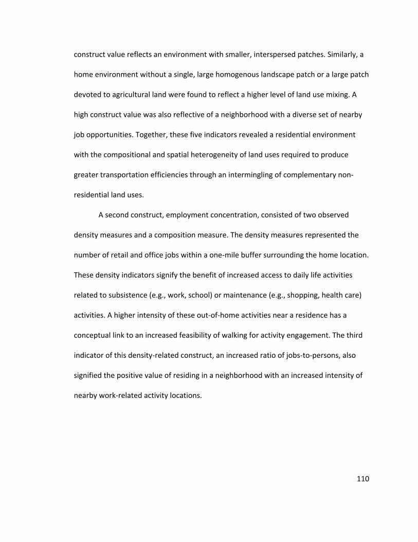
110

construct value reflects an environment with smaller, interspersed patches. Similarly, a

home environment without a single, large homogenous landscape patch or a large patch

devoted to agricultural land were found to reflect a higher level of land use mixing. A

high construct value was also reflective of a neighborhood with a diverse set of nearby

job opportunities. Together, these five indicators revealed a residential environment

with the compositional and spatial heterogeneity of land uses required to produce

greater transportation efficiencies through an intermingling of complementary non-

residential land uses.

A second construct, employment concentration, consisted of two observed

density measures and a composition measure. The density measures represented the

number of retail and office jobs within a one-mile buffer surrounding the home location.

These density indicators signify the benefit of increased access to daily life activities

related to subsistence (e.g., work, school) or maintenance (e.g., shopping, health care)

activities. A higher intensity of these out-of-home activities near a residence has a

conceptual link to an increased feasibility of walking for activity engagement. The third

indicator of this density-related construct, an increased ratio of jobs-to-persons, also

signified the positive value of residing in a neighborhood with an increased intensity of

nearby work-related activity locations.

111

Figure 5: Second-Order Latent Construct Reflecting a Smart Growth Neighborhood

The third first-order construct reflects elements of each built environment

dimension including urban design and the transportation system. Specifically, each of

the three indicators are associated with the provision of a street design conducive to a

highly walkable residential environment. This construct is reflected by a high percentage

of four-way intersections, which create a traditional street network design, and a high

percentage of streets with strong sidewalk coverage. Although listed as a composition

measure, a positive value for the indicator of retail land use patches denotes the

importance of a patchier landscape with smaller block sizes to this identified pedestrian-

oriented design construct.

112

A second-order smart growth neighborhood was strongly reflective of a positive

value in each of these described first-order latent constructs. The factor describing a

home environment with a walkable and traditional street network design was the

strongest predictor of a smart growth neighborhood (β=0.85), followed by the land

development pattern constructs of land use mix (β=0.63) and density (β=0.53). In sum,

these three first-order constructs indicate a home environment characterized by a

compact and complex land development pattern with a high intensity of nearby non-

residential activity locations and a pedestrian-oriented street network design.

4.4.2 Path analysis of home-based pedestrian travel

An examination of the structural model reveals that residing in a smart growth

neighborhood has a strong positive direct effect on the household-level decision to

participate in one or more home-based walk trips for transportation (β=0.22) or

discretionary (β=0.16) purposes. Furthermore, residing in a smart growth neighborhood

had a negative direct influence on the average home-based trip distance for all

household travel (β=-0.40). In fact, these paths from the second-order construct to the

three home-based travel behaviors represented the largest standardized direct effect of

any modeled determinant; however, caution must be stressed when providing

conclusions based solely on the magnitude of direct effects (Van Acker et al., 2007; de

Abreu e Silva, et al., 2012a). Accordingly, Table 14 provides an overview of the direct

and total effects of the second-order smart growth construct as well as exogenous

113

sociodemographic and transportation characteristics on the two modeled binary home-

based walk trip outcomes.

Table 14: Standardized Direct, Indirect, and Total Effects of the Structural Equation Model

Indicator Name

Walk Transportation Purposes

Walk Discretionary Purposes

Direct Indirect Total Direct Indirect Total

Built Environment Characteristics

Smart growth neighborhood 0.22 0.04 0.27 0.16 0.02 0.18

Sociodemographic and Economic Characteristics

Number of children under 6 years 0.05 0.01 0.05 Number of children 6 years or older 0.16 0.05 0.21 0.06 0.04 0.10 Number of adults 0.09 0.08 0.18 0.07 0.08 0.15 Annual income: Under $25,000 --- --- --- --- --- --- Annual income: $25,000 to $49,999 -0.02 0.00 -0.02 Annual income: $50,000 to $99,999 -0.05 0.04 -0.01 Annual income: $100,000 or more -0.06 0.05 -0.01 Household workers: 0 --- --- --- --- --- --- Household workers: 1 0.01 -0.04 -0.03 -0.03 -0.03 -0.06 Household workers: 2 0.01 -0.04 -0.04 -0.04 -0.03 -0.08 Household workers: 3 or more -0.04 -0.02 -0.06 -0.04 -0.02 -0.06 Education: High school diploma or less --- --- --- --- --- --- Education: Associate’s degree or credits -0.02 -0.01 -0.03 Education: Bachelor’s degree 0.03 -0.04 -0.01 Education: Graduate degree 0.05 -0.06 -0.01

Transportation Characteristics

Vehicles per licensed driver -0.05 -0.07 -0.11 Transit passes per adult -0.03 -0.05 -0.08 Bikes per person 6 years or older 0.04 0.03 0.07

Notes: Dashes (---) indicate the reference case. Empty cell indicates pathway between variables was not specified.

Following the proposed conceptual framework, the observed sociodemographic

and economic characteristics were directly predictive of the residential environment in

addition to the average home-based trip distance for all travel modes and decisions to

walk for transportation or discretionary purposes. Therefore, the total effect of all

household-level socio-economic and transportation characteristics also included the

114

potential mediating impacts of the home built environment and average trip distance on

the two pedestrian travel outcomes. Likewise, the total effect of a smart growth

neighborhood on walking behaviors accounted for the indirect path through average

home-based trip distance, which is theorized to directly influence the modal decision to

walk.

In terms of a household making one or more walk trips for either subsistence or

maintenance activities, the total effect of residing in a neighborhood characterized by

smart growth features had the greatest standardized impact in the final SEM estimation.

Household composition factors related to the number of children over six years of age

and adults also had a strong positive effect on conducting at least one home-based walk

trip for transportation purposes, which may include either school- or work-related

travel. An increase in the number of children under six years old had a marginally

significant positive effect on walking for subsistence or maintenance activities. In

contrast, a household with an increase in the number of workers or annual income were

less likely to walk for transportation purposes, with the former predictor having a

stronger total effect. As expected, the number of household vehicles per licensed driver

had a significant, negative direct and total effect on non-discretionary walking; whereas,

an increase in the number of bikes per individual six years of age or older had a positive

total standardized effect.

The total standardized effect of residing in a smart growth neighborhood on the

household-level choice to participate in at least one walk trip for discretionary purposes

115

was also positive, albeit smaller in magnitude than the paths to non-discretionary

walking. An increase in the number of household adults and children six years of age or

older also had positive direct, indirect, and total standardized effects on the decision to

participate in at least one daily walk trip for discretionary purposes. In contrast, an

increase in the number of household workers had a significant, negative direct and total

effect on walking. While the direct effect of having at least one household member with

a graduate degree had a positive impact on discretionary walking, the total effect of this

indicator became negative once the indirect effects were modeled. Finally, households

with a higher proportion of transit passes per adult were less likely to have taken at

least one walk trip for discretionary activities.

4.5 Conclusions

This study introduced a second-order latent construct reflecting three key tenets

of smart growth land development and established its link to pedestrian travel in a

conceptual model. While planning literature has long hypothesized this transportation-

land use connection, prior studies have inadequately addressed the multicollinearity of

many built environment indicators and further misunderstood the contribution of these

spatial phenomenon in a multidirectional modeling structure. To the first point, this

study utilized latent factor analyses in finding that development patterns related to land

use mix and density as well as urban design and transportation system features together

explain variation in residential environments. Thus, a neighborhood with a walkable

116

environment characterized by a traditional street network design with strong sidewalk

coverage and localized retail, mixed land development patterns represented by both

complementary and spatially interspersed land use patches, and compact setting with

high employment intensity indicated a smart growth neighborhood. When measured at

the residential location, this latent construct had a stronger direct and total effect on

increasing home-based, household-level pedestrian travel than those socio-economic

characteristics tested in the theoretical model. Findings from the SEM corroborate

generalizations of transportation-land use literature stating that trip distance is largely a

function of the built environment, while mode choice is a function of both

sociodemographic and built environment characteristics (Ewing, et al., 2015).

Evidence from this study may be used to help inform pedestrian planning policy

and guide practice away from contentious land development debates. Analysis of

residential built environments both within and outside of Portland and its metropolitan

region resulted in the creation of a smart growth construct accounting for the variation

in urban, suburban, and rural communities. To combat urban sprawl with urban infill

and suburban retrofitting policies, this study has provided planners with an identified

set of indicators that may be toggled to improve built environment efficiencies and

consequently encourage physically active modes of travel. Of further interest, the

density-related latent construct was the weakest indicator of a smart growth

neighborhood and had the notable omission of any population density measure. While

increasing the level of employment opportunities in a community presents its own set

117

of difficulties, the strength of the other first-order factors suggests planners may

achieve smarter growth by framing land development debates toward a dialogue of how

development may be spatially configured and designed to promote walkability.

Moreover, study findings support urban infill policies aimed at siting residential

developments in existing employment districts as a favorable smart growth strategy.

While this study has several exciting implications for policy and practice,

research extensions should also address its limitations to offer further direction on how

residential environments may be developed to encourage transportation-related

physical activity. Foremost, the study’s cross-sectional research design limits the ability

to establish causal inference and adequately control for residential self-selection bias in

which a household chooses where to reside based on its travel preferences (Cao &

Chatman, 2016). Yet, topic overviews have found that built environment characteristics

influence active travel after accounting for any residential sorting (Cao, 2015).

Additional sociodemographic variables, which may be assessed as a formative construct

(e.g., Banerjee & Hine, 2016), and contextual factors (e.g., slope, weather) should be

explored in alternative model specifications. Although the table of built environment

indicators is extensive, the absence of psychosocial variables describing individual

perceptions of the built environment and travel bias study findings. Relatedly, while a

household-level analysis explains some inter-household dynamics, an adoption of a

hierarchical SEM framework would enable an understanding of this transportation-land

use connection at the level of the decision-maker. Further, while this SEM application

118

measured the built-environment at a pedestrian scale, more work is needed to

understand the impact of alternative spatial scales for both operationalizing the

proposed smart growth construct and measuring its contribution to travel behavior.

Nevertheless, while some methodological limitations are inherent to any modeling

application, this study delivers an empirical analysis in a multidirectional framework that

highlights the continued prospect for smart growth land use policies to positively affect

pedestrian travel outcomes.

119

Chapter 5: Operationalizing the Neighborhood Effects of the Built Environment on

Travel Behavior

5.1 Introduction

Study of the transportation-land use connection has an established evidence

base, which via contributions from the public health field has only started to investigate

the impact of the built environment on walking as a mode of transportation and physical

activity (Saelens & Handy, 2008). Prior transportation planning research almost

exclusively investigated auto-related travel using regional built environment measures;

however, most recent studies have adopted more suitable neighborhood-level

indicators to evaluate any environmental connections to active transportation (Handy,

et al., 2002). This shift in emphasis toward a rounded assessment of travel behavior is

largely attributable to the advent of geographic information systems (GIS) and the

pairing of disaggregate land use data with household travel diary datasets (Boarnett,

2011) as well as an increased adoption in policies directed toward achieving goals of

livability. In all, these technological advancements coupled with multidisciplinary

interest have helped to guide the adoption of integrated transportation-land use

programs aimed at creating walkable, activity-friendly communities.

Policies and programs that facilitate active transportation or physical activity are

generally place-dependent and therefore linked to a person’s physical surroundings

(Sallis 2009). Yet, conceptualizing the built environment with a set of key indicators

120

reflecting the dimensions of land development pattern, urban design, and

transportation system remains a complicating factor in understanding the strength of

this accepted relationship (Frank & Engleke, 2001). Although improvements in data

quality and availability have aided this nontrivial task, many adopted measures are still

inadequate for studying the link between the built environment and all modes of

transportation (Handy, et al., 2002). A concern for practitioners and researchers alike

who are interested in understanding how changes to these different dimensions of the

built environment can moderate sustainable travel behaviors. Nonetheless, while

representation of these dimensions with a succinct collection of contextual indicators

continues to be a challenging endeavor, past studies generally reveal a positive

association between the built environment and travel (Ewing & Cervero, 2010).

However, given the wide variation in spatial boundaries chosen to operationalize these

myriad measures, the extent of any environmental association with active or auto-

related travel remains somewhat unclear (Clark & Scott, 2014).

Inconsistencies in the modelled neighborhood effects of the built environment

on travel behavior that result from the measurement of a traveler’s environmental

context with different spatial boundaries is defined as the modifiable areal unit problem

(Hess, et al., 2001). Given the fact that this problem may arise from representing

different dimensions with particular levels of aggregation and zoning systems, it is

surprising that this methodological issue has not received greater attention in the

transportation-land use evidence base (Kwan & Weber, 2008). Additionally, the

121

prospect for scale-related decisions to distort the significance or degree of any theorized

interaction confounds any understanding of how the physical context near each trip end

effects an individual’s travel behavior for different trip purposes. In response to these

identified needs, this article investigates how the operationalization of the built

environment at each trip end potentially affects the connection of this multidimensional

depiction of place to individual-level travel mode choices across trip purposes.

5.2 Geographic Scale Variation in Transportation-Land Use Research

The spatial nature of selecting a geographic scale to represent the built

environment is inherent to studies testing the relationships between land development

patterns and travel (Hess, et al., 2001). Contextual influences of travel behavior such as

the built environment often stretch continuously across study areas, presenting a set of

research challenges related to the complexity of dividing its spatial effect into distinct,

overlapping, or multilevel units of analysis (Openshaw, 1983; Kwan, 2012). Expectedly,

transportation-land use research has investigated the built environment’s impact on

travel by using measures operationalized at varying spatial scales (Handy, et al., 2002),

with few studies experimenting with scale variation (Boarnet, 2011). A chief concern of

this inattention to scale selection is the reflection of built environment aspects with

unsuitable spatial units that result in inconsistent study findings and policy implications

(Frank, 2000).

122

In geographic and statistical literature, the sensitivity of analytic results to the

definition of spatial units for collecting and reflecting these neighborhood effects refers

to the modifiable areal unit problem (MAUP; Fotheringham & Wong, 1991). The MAUP

consists of two components, scale and zoning effects, which arise from the subjective

decision of boundary delineations in reporting contextual influences. The scale effect

describes the sensitivity or unreliability of built environment measures due to changes

in the size of the selected geographic unit of analysis (Gehlke & Biehl, 1934; Openshaw,

1983). Therefore, any variation in the association between the built environment and

travel may simply be the result of adopting smaller or larger scales to reflect the former

phenomenon. In contrast, the zoning effect arises from the multitude of ways to

configure a spatial boundary or neighborhood at each level of aggregation (Jelinski &

Wu, 1996). The following subsections, organized by the operationalization of the built

environment with fixed or sliding scales (Guo & Bhat, 2007; Gehrke & Clifton, 2016),

provide a review of previous studies of scale variation to recognize its influence on

understanding the built environment determinants of travel.

5.2.1 Fixed geographic scales

Describing a built environment aspect within a predefined set of distinct,

adjoining boundaries represents the application of a fixed geographic scale to study

neighborhood effects. The implementation of a fixed zonal system to operationalize

built environment measures is typically due to analytical convenience, data availability,

123

and the attractiveness of a prevailing hierarchical structure (Kwan & Weber, 2008).

Examples of fixed zonal systems include administrative, statistical, and artificial

boundaries (Gehrke & Clifton, 2016). The use of statistical boundaries (e.g., census

units) to describe the local built environment is pervasive in travel behavior research

because of the ease of obtaining sociodemographic and economic data for the same

boundary (Guo & Bhat, 2007) and their objective approximation of the neighborhood

unit (Manaugh & Kreider, 2013). However, variation in the spatial scale of contiguous

statistical boundaries has directed the increased adoption of artificial boundaries (e.g.,

grid cells) that assess the neighborhood effect of the built environment by generating a

uniformed, synthetic zoning system (Krizek, 2003b).

In an early study of the MAUP within transportation-land use research, Zhang

and Kukadia (2005) utilized three statistical and five artificial zoning systems to

operationalize the built environment around an individual’s residence to assess its

impact on travel mode choice. Considering three common measures, the authors noted

tractable and stable estimation results of home-based travel when operationalizing the

built environment with artificial boundaries. In a study of active travel in Halifax, Clark

and Scott (2014) compared the use of statistical and artificial boundaries to

operationalize five land development pattern, urban design, and transportation system

characteristics of the traveler’s home environment. Their study findings corroborate the

prior work by suggesting the MAUP has a significant influence on the relationship

between the built environment and active travel. Other studies outside the United

124

States (Duncan, et al., 2010; Learnihan, et al., 2011; Mitra & Buliung, 2012) similarly

employed statistical boundaries to understand the impact of their adoption for

quantifying the neighborhood effect of the built environment on physical activity.

Investigating land use mix, Duncan et al. (2010) measured development patterns at four

census scales and found adjusting for scaling effects improved the phenomenon’s

association with walk trip duration. Learnihan et al. (2011) examined the impact of four

walkability indicators near the residence on walking for transport and recreation;

whereas, Mitra and Buliung (2012) considered the influence of a greater set of

contextual indicators near the home location and destination on school-related walking

and bicycling. In addition, Houston (2014) found evidence of zoning effects, by using

three artificial boundaries to estimate the neighborhood effects of five environmental

measures at home and non-home locations on moderate and physical activity bouts.

Overall, studies examining the MAUP through the adoption of fixed geographic

scales confirm the influence of scaling and zoning effects on understanding the

transportation-land use connection. Zoning effects result from the seemingly arbitrary

placement of a trip end, which may be closer to the center or perimeter of the

partitioned space, inside the unit of analysis (Oliver, et al., 2007; Mitra & Buliung, 2012).

For this reason and the wider availability of disaggregate data that reduces the scaling

effect (Clark & Scott, 2014), recent studies have also generally operationalized the built

environment with sliding scales.

125

5.2.2 Sliding geographic scales

Measuring an individual’s contextual surroundings at a given activity location by

using objective distance- or time-related boundaries indicates the adoption of a sliding

geographic scale (Guo & Bhat, 2007; Gehrke & Clifton, 2014). Sliding scales offer an

individual-centric operationalization of the neighborhood concept that tries to explain

those built environment aspects most likely to affect travel decisions (Gehrke & Clifton,

2016). The creation of areal buffers extending from an activity location, a sliding scale

application, permits the formation of overlapping spatial boundaries that enable

variation in neighborhood delineations. Yet, the assumption that the environment

within this circular-unit representation is equally consequential in all directions to the

decision-making process and an insensitivity to the physical constraints to local access

presented by nearby natural and artificial boundaries limits the appeal of areal buffers

(Guo & Bhat, 2007). Network bands, which confine the neighborhood boundary to

include only the area that an individual can hypothetically travel in all directions along a

street network, reflect a more nuanced way to operationalize the built environment

with a sliding geographic scale (Frank, et al., 2008).

Utilizing areal buffers and network bands at four spatial extents, Forsyth et al.

(2007) found only modest relationships between physical activity and housing,

population, employment, and activity density at the home location. The authors were

unable to conclude at what scale density matters most for physical activity and

identified the importance of examining other environmental features for increasing

126

walking rates. Operationalizing population density as well as business intensity and

intersection density with four areal buffer extents, Boone-Heinonen et al. (2010)

revealed higher physical activity levels were generally associated with the latter two

aspects at smaller spatial extents. However, in a Seattle-based study of the built

environment and physical activity in older adults, Berke et al. (2007) found a significant

association between increased walking for exercise and a walkability index comprised of

eight features including housing and retail store density, across three areal buffers. Kerr

et al. (2014) echoed this finding in a San Diego-based study of physical activity in older

women, but acknowledged small effect sizes. This last study, like studies by Forsyth et

al. (2007) and Learnihan et al. (2013), used network bands to assess the impact of

scaling effects on the relationship between the built environment at the home location

and walking. In a study of travel mode choice and land use mixing, Gehrke and Clifton

(2014) explored the scaling and zoning effects of seven land composition measures

operationalized at the trip origin and destination with two statistical boundaries and

two network bands. Their study found land use diversity at the trip destination had a

positive relationship with walking and bicycling when calculated at the larger spatial

extents.

Sliding scale representations of the built environment represent a

methodological and conceptual improvement over fixed scaled delineations of the

neighborhood concept. Foremost, by only measuring the built environment that

immediately extends from a given activity location, areal buffers and networks bands

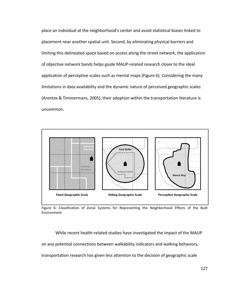
127

place an individual at the neighborhood’s center and avoid statistical biases linked to

placement near another spatial unit. Second, by eliminating physical barriers and

limiting this delineated space based on access along the street network, the application

of objective network bands helps guide MAUP-related research closer to the ideal

application of perceptive scales such as mental maps (Figure 6). Considering the many

limitations in data availability and the dynamic nature of perceived geographic scales

(Arentze & Timmermans, 2005), their adoption within the transportation literature is

uncommon.

Figure 6: Classification of Zonal Systems for Representing the Neighborhood Effects of the Built Environment

While recent health-related studies have investigated the impact of the MAUP

on any potential connections between walkability indicators and walking behaviors,

transportation research has given less attention to the decision of geographic scale

128

selection. The continued variation in the choice of scale and spatial extent to study this

relationship increases the likelihood that the MAUP may have affected study findings

and creates uncertainty in the extent of any modeled relationship (Clark & Scott, 2014).

For this reason, recent transportation studies (Mitra & Buliung, 2012; Clark & Scott,

2014) have started to consider the implications of scale and zoning effects on

recognized transportation-land use connections. Extending these efforts, this study

operationalizes an extensive list of built environment measures with a wide range of

zonal systems to (a) analyze the connection between travel mode choice and the built

environment at varying fixed and sliding scales, and (b) investigate the contribution of

the built environment at each trip end for adult travel to work and nonwork locations.

5.3 Data and Methods

5.3.1 Travel behavior data and study area

This study used transportation data provided by an activity-travel survey of

46,414 individuals from 19,932 randomly sampled households in Oregon between 2009

and 2012. The Oregon Household Activity Survey was a one-day diary of weekday travel

reported by a chosen household member who detailed information on the activity

locations, trip purposes, and modes of all out-of-home travel conducted by their

household as well as sociodemographic and economic characteristics of the household

and its individual members. The travel behaviors and patterns of a subsample of 3,139

129

adults from 1,912 home locations within the City of Portland, who performed 4,745

home-based trips to a destination inside the three-county Portland metro region, were

analyzed in this study. Table 15 describes the study sample.

Of these home-based unlinked trips, most individuals traveled to their activity

location as either the driver or passenger of a private vehicle (77%), while other

travelers selected a more active mode such as walking (12%) or bicycling (8%). Nearly

one-half (47%) of these recorded out-of-home trips were related to carrying out

subsistence activities such as commuting to work or school, while the remaining

nonwork trips were related to conducting travel for mandatory (e.g., shopping) or

discretionary (e.g., recreation) purposes. Overall, the average distances for home-based

work (HBW) and home-based nonwork (HBNW) trips were 4.70 and 2.41 miles,

respectively. This relationship was consistent across the different travel modes for the

study subsample. The average HBW trip distance was 6.76 miles for individuals riding

public transit, 5.09 miles for automotive travel, 2.79 miles for bicyclists, and 0.64 miles

for pedestrians. As for nonwork trips, on average, an individual traveled 4.35 miles when

using transit, 2.78 miles when driving, 1.54 miles when bicycling, and 0.33 miles when

walking from their residence to an out-of-home location.

Table 15: Descriptive Statistics of the Study Sample

Variable Name n % Mean St. Dev. Min Max

Individual Characteristics (n = 3,139)

Gender: Female 1,704 0.54 --- --- 0.00 1.00 Age: 16 to 29 years old 339 0.11 --- --- 0.00 1.00 Age: 30 to 44 years old 764 0.25 --- --- 0.00 1.00

130

Age: 45 to 64 years old 1,472 0.48 --- --- 0.00 1.00 Age: 65 years or older 521 0.17 --- --- 0.00 1.00 Education: High school diploma or less 494 0.16 --- --- 0.00 1.00 Education: Associate’s degree or credits 657 0.21 --- --- 0.00 1.00 Education: Bachelor’s degree 985 0.32 --- --- 0.00 1.00 Education: Graduate degree 989 0.32 --- --- 0.00 1.00 Employed: Part- or full-time 2,193 0.70 --- --- 0.00 1.00 Student: Part- or full-time 314 0.10 --- --- 0.00 1.00 Disability affecting travel 202 0.06 --- --- 0.00 1.00 Driver’s license 2,878 0.92 --- --- 0.00 1.00 Parking provided at no charge by employer 1,621 0.68 --- --- 0.00 1.00 Transit pass 629 0.20 --- --- 0.00 1.00 Transit pass provided at no charge by employer

293 0.12 --- --- 0.00 1.00

Bike 1,248 0.40 --- --- 0.00 1.00

Household Characteristics (n = 1,912)

Number of children under 6 years old --- --- 0.13 0.42 0.00 4.00 Number of children 6 to 15 years old --- --- 0.25 0.62 0.00 4.00 Number of adults --- --- 1.85 0.73 1.00 7.00 Number of part- or full-time workers --- --- 1.84 0.69 1.00 7.00 Non-related household 69 0.04 --- --- 0.00 1.00 Annual income: Under $25,000 247 0.14 --- --- 0.00 1.00 Annual income: $25,000 to $49,999 381 0.22 --- --- 0.00 1.00 Annual income: $50,000 to $99,999 696 0.40 --- --- 0.00 1.00 Annual income: $100,000 or more 431 0.25 --- --- 0.00 1.00 Oldest adult: 16 to 29 years old 63 0.03 --- --- 0.00 1.00 Oldest adult: 30 to 44 years old 399 0.21 --- --- 0.00 1.00 Oldest adult: 45 to 64 years old 962 0.51 --- --- 0.00 1.00 Oldest adult: 65 years or older 467 0.25 --- --- 0.00 1.00 Highest education: High school diploma or less 148

0.08 --- ---

0.00 1.00

Highest education: Associate’s degree 340 0.18 --- --- 0.00 1.00 Highest education: Bachelor’s degree 595 0.31 --- --- 0.00 1.00 Highest education: Graduate degree 826 0.43 --- --- 0.00 1.00 Household vehicles per licensed driver --- --- 0.92 0.48 0.00 3.00 Household transit passes per adult --- --- 0.20 0.34 0.00 1.00 Household bikes per person 6 years or older ---

--- 0.64 0.76 0.00 13.00

5.3.2 Built environment data and measurement

To supplement these characteristics of the traveler and his/her home-based

travel behavior, information describing the land development patterns, urban design,

and transportation systems near an individual’s residence and his/her destination were

131

collected. Land development patterns denote both the density of activities within a

neighborhood and their composition or spatial configuration in terms of land use mixing

(Gehrke & Clifton, 2017a; Gehrke & Clifton, 2017b). Reduced trip lengths and

subsequent increases in travel mode availability are posited to be associated with an

intensification in the diversity and interspersion of local activities or land uses (Frank &

Engelke, 2001). Urban design, on the other hand, describes the arrangement and

appearance of various environmental features; whereas, the transportation system

details the physical infrastructure and performance of the various systems presented to

the traveler (Saelens & Handy, 2008). Features in the former dimension describe the

desirability for travel and are more likely to affect walking and cycling in which a person

moves through a setting at a slower rate, while transportation systems are integral to

providing connections between trip origins and destinations (Frank & Engelke, 2001).

A wide-ranging list of indicators for each of these dimensions was measured for

this study (Table 16). These 57 variables were calculated using secondary land use data

provided by the 2011 Portland Metro Regional Land Information System, 2010 US

Census, 2014 Longitudinal Employer-Household Dynamics (LEHD) Program, and 2010

Topologically Integrated Geographic Encoding and Referencing files. Density variables

describe the number of housing units, persons, and employment activities per acre.

Land use composition indicators assess the balance in jobs and housing, diversity in

employment activities, relative proportion of land use types, and frequency of

landscape patches within a neighborhood. The distribution of multiple land use types

132

was assessed using two versions of the land use entropy index (Cervero, 1989), balance

(Bhat & Gossen, 2004), and activity-related complementarity (Gehrke & Clifton, 2017a)

measures. The final pattern aspect, configuration, denotes the shape, size, and

arrangement of landscape patches in a neighborhood (Clifton, et al., 2008). The

contagion index (Li & Reynolds, 1994; Gehrke & Clifton, 2017a) is a configuration

measure differentiating neighborhoods with a small number of contiguous patches from

those areas with an intermixing of dissimilar patches. The dozen urban design and

transportation system indicators reflect attempts to identify the permeability of the

street network system and the relative ease of either passive or active travelers to move

throughout their physical environments. The alpha, beta, cyclomatic, and gamma

indices noted in Table 16 are network structure and connectivity indices introduced in

prior transportation-land use studies (Dill, 2004; Levinson, 2012; Song, et al., 2013b).

In this study, all described built environment indicators were calculated at both

the residence and trip destination. To recognize the potential impact of the MAUP, the

built environment at each trip end was operationalized using 12 different combinations

of zonal systems and scale extents. The first pair of geographies reflect statistical zonal

systems measuring the context with spatial extents at the US Census tract and block

group. Adopting another pairing of fixed scale geographies, the built environment was

also measured using artificial boundaries where grid cell systems of one-quarter-mile

and one-mile edges were casted over the study area. For both fixed scale strategies of

built environment measurement, the home and trip destination were assigned the

133

attributes of the statistical or artificial boundary in which they were located. A second

measurement strategy used two sliding geographic scales, areal buffers and network

bands, to measure the built environment around the origin and destination at one-

quarter-, one-half-, three-quarter-, and one-mile spatial extents. Disaggregate data were

simply summarized to the geography of interest; whereas, data from the US Census and

LEHD datasets were provided at the block-level and aggregated to the respective

neighborhood representation using a proportional split method. While use of the

smallest available spatial unit limits MAUP-related sensitivity, one assumption of this

strategy is the uniform dispersion of all attributes in the selected geographic boundary

(Schlossberg, 2003).

Table 16: Description of Built Environment Indicators

Variable Name Description Sourcea

Land Development Patterns: Density

Housing density Number of housing units per acre C Persons density Number of persons per acre C Jobs density Number of jobs per acre L Activity density Sum of persons and jobs per acre C, L Retail jobs density Number of retail jobs per acre L Office jobs density Number of office jobs per acre L Industrial jobs density Number of industrial jobs per acre L Service jobs density Number of service jobs per acre L Entertainment jobs density Number of entertainment jobs per acre L

Land Development Patterns: Land use mix, Composition

Jobs-housing balance Ratio of jobs-to-housing units C, L Employment entropy Entropy index based on five job sub-categories L Land use percent: Residential Percent of land area classified as residential R Land use percent: Retail Percent of land area classified as retail R Land use percent: Manufacturing Percent of land area classified as manufacturing R Land use percent: Utilities Percent of land area classified as utilities R Land use percent: Entertainment Percent of land area classified as entertainment R Land use percent: Education Percent of land area classified as education R Land use percent: Construction Percent of land area classified as construction R

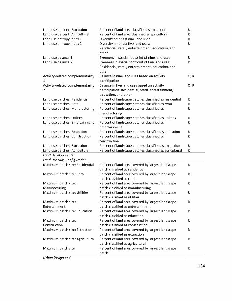
134

Land use percent: Extraction Percent of land area classified as extraction R Land use percent: Agricultural Percent of land area classified as agricultural R Land use entropy index 1 Diversity amongst nine land uses R Land use entropy index 2 Diversity amongst five land uses:

Residential, retail, entertainment, education, and other

R

Land use balance 1 Evenness in spatial footprint of nine land uses R Land use balance 2 Evenness in spatial footprint of five land uses:

Residential, retail, entertainment, education, and other

R

Activity-related complementarity 1

Balance in nine land uses based on activity participation

O, R


Balance in five land uses based on activity participation: Residential, retail, entertainment, education, and other

O, R

Land use patches: Residential Percent of landscape patches classified as residential R Land use patches: Retail Percent of landscape patches classified as retail R Land use patches: Manufacturing Percent of landscape patches classified as

manufacturing R

Land use patches: Utilities Percent of landscape patches classified as utilities R Land use patches: Entertainment Percent of landscape patches classified as

entertainment R

Land use patches: Education Percent of landscape patches classified as education R Land use patches: Construction Percent of landscape patches classified as

construction R

Land use patches: Extraction Percent of landscape patches classified as extraction R Land use patches: Agricultural Percent of landscape patches classified as agricultural R

Land Developments: Land Use Mix, Configuration

Maximum patch size: Residential Percent of land area covered by largest landscape patch classified as residential

R

Maximum patch size: Retail Percent of land area covered by largest landscape patch classified as retail

R

Maximum patch size: Manufacturing

Percent of land area covered by largest landscape patch classified as manufacturing

R

Maximum patch size: Utilities Percent of land area covered by largest landscape patch classified as utilities

R

Maximum patch size: Entertainment

Percent of land area covered by largest landscape patch classified as entertainment

R

Maximum patch size: Education Percent of land area covered by largest landscape patch classified as education

R

Maximum patch size: Construction

Percent of land area covered by largest landscape patch classified as construction

R

Maximum patch size: Extraction Percent of land area covered by largest landscape patch classified as extraction

R

Maximum patch size: Agricultural Percent of land area covered by largest landscape patch classified as agricultural

R

Maximum patch size Percent of land area covered by largest landscape patch

R

Urban Design and

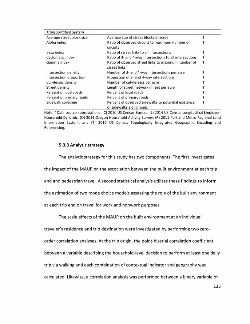
135

Transportation System

Average street block size Average size of street blocks in acres T Alpha index Ratio of observed circuits to maximum number of

circuits T

Beta index Ratio of street links to all intersections T Cyclomatic index Ratio of 3- and 4-way intersections to all intersections T Gamma index Ratio of observed street links to maximum number of

street links T

Intersection density Number of 3- and 4-way intersections per acre T Intersection proportion Proportion of 3- and 4-way intersections T Cul-de-sac density Number of cul-de-sacs per acre T Street density Length of street network in feet per acre T Percent of local roads Percent of local roads T Percent of primary roads Percent of primary roads T Sidewalk coverage Percent of observed sidewalks to potential existence

of sidewalks along roads T

Note: a Data source abbreviations: (C) 2010 US Census Bureau, (L) 2014 US Census Longitudinal Employer-Household Dynamic, (O) 2011 Oregon Household Activity Survey, (R) 2011 Portland Metro Regional Land Information System, and (T) 2010 US Census Topologically Integrated Geographic Encoding and Referencing.

5.3.3 Analytic strategy

The analytic strategy for this study has two components. The first investigates

the impact of the MAUP on the association between the built environment at each trip

end and pedestrian travel. A second statistical analysis utilizes these findings to inform

the estimation of two mode choice models assessing the role of the built environment

at each trip end on travel for work and nonwork purposes.

The scale effects of the MAUP on the built environment at an individual

traveler’s residence and trip destination were investigated by performing two zero-

order correlation analyses. At the trip origin, the point-biserial correlation coefficient

between a variable describing the household-level decision to perform at least one daily

trip via walking and each combination of contextual indicator and geography was

calculated. Likewise, a correlation analysis was performed between a binary variable of

136

the individual-level decision to participate in a walk trip and each combination of

indicator and boundary to describe the scaling effect of the MAUP on the built

environment near the trip destination. The outcome of this initial analysis provides

insight into the scale effect through the identification of visual trends in the statistical

significance and magnitude of these 1,392 associations. An understanding of the

potential zoning effects of the built environment connection with active travel was

investigated by comparing these associations found at each trip end across comparable

spatial extents but different zonal systems (i.e., one-mile areal buffer versus one-mile

network band). After this analysis of the MAUP’s effect on the built environment

connection to pedestrian travel, the pairing of indicator and geographic boundary at

each trip end with the strongest absolute magnitude was selected for further testing in

the two mode choice models.

Discrete choice modeling (DCM) is an established strategy for empirically

modeling the relative importance of individual and alternative characteristics in travel

mode choice (Cervero, 2002; Handy, et al., 2002). In this framework, the mode choice

set considered by a decision maker comprises an exhaustive, finite list of four mutually

exclusive alternatives: auto, transit, bicycle, and walk. The individual is described by a

set of personal, household, and transportation-related characteristics described

previously in Table 15, while the alternative and contextual characteristics include travel

time, travel cost, and the built environment at each activity location. Adoption of

disaggregate DCM offers the ability to represent changes in mode choice behavior

137

related to varying individual, alternative, and contextual features and modify the choice

set to only include those alternatives available to an individual (Ben-Akiva & Lerman,

1985; Koppelman & Bhat, 2006; Train, 2009).

Travel time, measured in minutes, was an alternative-specific attribute

calculated using the 2010 travel skims modeled by Portland Metro at the traffic analysis

zone (TAZ). Midday and peak period travel times for each feasible alternative were

determined by matching each trip end to its respective TAZ and then linking the trip

departure times to the appropriate time-of-day skim. The feasible mode choice set was

defined by the following assumptions. Since no distinction was made between auto-

related travel as a driver or passenger, the only restriction for this alternative was that

the ratio of licensed drivers per household vehicle must exceed zero. For transit, which

entailed bus and rail-based modes, availability was predetermined for each TAZ

geography in the modeled skims. Bicycling and walking were considered as available

modes if the individual’s trip could be conducted in two hours assuming an average

travel speed of 9.0 and 3.5 miles per hour, respectively. An additional constraint was

placed on bicycle availability if the number of household bikes was zero. Travel costs

were not calculated for observed or alternative trips using an active transportation

mode; however, the costs associated with auto and public transit use were modeled and

based on assumptions previously described elsewhere (Singleton & Wang, 2014).

The application of this DCM framework enabled a cumulative strategy for

assessing how land development pattern, urban design, and transportation system

138

features at the trip origin and destination affect home-based modal decisions for work

and nonwork travel. First, a reduced model was estimated using individual- and

household-level attributes of the traveler and alternative-specific characteristics of the

trip. Second, built environment features measured at the residence were added to the

base model. These indicators, operationalized at a boundary determined by the earlier

MAUP-related analysis, were added to the base model by a forward selection process in

which the log-likelihood of the newly-specified model was then tested against the base

model’s fit. The variable that produced an expanded model with the best model fit was

retained. This iterative process continued until the addition of a contextual feature to

the previous model specification no longer produced a statistically significant

improvement according to the log-likelihood ratio test. The full model specification was

determined by repeating this step for all features measured at the trip destination. This

analytic strategy produced a base and full model of mode choice for HBW and HBNW

trip purposes that provides insight into the neighborhood effect of the built

environment on travel behavior.

5.4 Results

5.4.1 Scale and zoning effects

The magnitude and direction of the relationship between the 57 built

environment features measured at 12 geographies and pedestrian travel were

139

investigated to assess MAUP-related effects. Inspection of the scale effect of the built

environment at the trip origin is guided by the results of the correlation analysis in

Figure 7. Looking at the set of density measures, a consistently positive association was

found between the household decision to conduct at least one walk trip and an

increased intensity in activities within a residential neighborhood. Within sliding scale

zonal systems, the strength of the point-biserial correlation coefficient remained above

0.10 at each of the four spatial extents. A similar finding occurred within the two scale

extents for the statistical and artificial boundaries; however, operationalizing density

measures with a grid cell revealed a small and counterintuitive connection to the

household-level walking behavior.

Comparing land use mix measures operationalized with fixed scales, the effect

size and direction of correlation coefficients generally remained unchanged at the two

spatial extents. Consistency was also exhibited when the configuration measures related

to maximum patch size and the contagion index were measured using areal buffers or

network bands. Land use composition measures, however, showed signs of scaling

effects when measured with these two sliding scale representations. Using areal buffers,

both versions of the land use entropy index and activity-related complementarity

measure had strong, positive associations with walking at the smaller spatial extents,

but this effect size decreased as the zoning size increased. The flattening of this

connection due to increased aggregation levels has been noted elsewhere in the

literature (Zhang & Kukadia, 2005; Mitra & Buliung, 2012; Clark & Scott, 2014).

140

Interestingly, the adoption of network bands to represent street network connectivity

revealed two instances where this recognized trend was contradicted. The strength of

the relationship between the household-level decision to walk and the alpha and

gamma indices improved as the spatial extent increased. This discovery could be the

result of micro-level urban design features having a greater effect on walking when the

connectivity of a network extends and consequently increases the feasibility and

attractiveness of longer walk trips.

The scale effects of built environment measurement at the destination were also

examined (Figure 8), but the relationships between these features when measured at

this trip end and the individual-level decision to walk were not as robust. Density in

housing and employment in office or entertainment sectors exhibited scaling effects

when operationalized with artificial boundaries. Both land use entropy and the

maximum residential patch size were also impacted by increased aggregation levels

when measured by an areal buffer zoning system, while the former mix indicator also

suffered from scaling effects when operationalized using grid cells or network bands. In

contrast, the percent of residential or retail land uses in a neighborhood defined by

areal buffers had a diminishing strength of relationship with walking as the spatial

extent increased. Similar to the origin-related analysis, several connectivity indices

demonstrated an increased strength of relationship with walking as the spatial extent of

the areal buffer increased.

141

Visual inspection of Figure 7 and 8 can also deliver insight into the potential

zoning effects of the built environment connection to pedestrian travel. Unfortunately,

a more definitive assessment of the impact of zoning systems across fixed geographic

extents can only be achieved by comparing different orientations of the same zoning

system (Clark & Scott, 2014). One illustration of this strategy would be the placement of

numerous orientations of grid cells with one-mile edges over a trip end in order to

measure any changes in the strength of association due to the varying contexts enclosed

around the trip end. This study, instead, conducted a pseudo analysis of zoning effects

by comparing associations between walking and the built environment at identical

spatial extents for the two sliding geographic scales.

142

Figure 7: Zero-Order Correlation between Walking and Built Environment at Trip Origin (N = 1,912)

143

Figure 8: Zero-Order Correlation between Walking and Built Environment at Trip Destination (N = 4,745)

144

Overall, zoning effects were not apparent for those density indicators measured

at both the trip origin and destination. Comparison of mix measures operationalized

with areal buffers to network bands, in turn, showed more instances of zoning effects.

Measured at the home location, several composition indicators were impacted by

zoning system selection, including the land use and employment entropy indices,

activity-related complementarity, and jobs-housing balance measures. Beyond a set of

composition measures, two configuration measures describing the maximum size of a

residential or retail landscape patch in the neighborhood encircling the destination also

displayed zoning effects. As for the other built environment dimensions, measures of

the average city block size, alpha index, and gamma index were all impacted by zonal

configuration decisions at both trip ends. However, in line with the overall trend, zoning

effects appeared to be most prominent at the trip destination when analyzing the

neighborhood effects of the built environment on walking.

5.4.2 Travel mode choice

Extending the utility of these MAUP-related findings, a second analysis was

performed to understand the neighborhood effects of the built environment at each trip

end on travel mode choice. Adding this second component provided behavioral

complexity to this study by (a) accounting for individual, household, and transportation

characteristics that may confound any observed active transportation-land use

association and (b) refining an individual’s choice set to only consider realistic travel

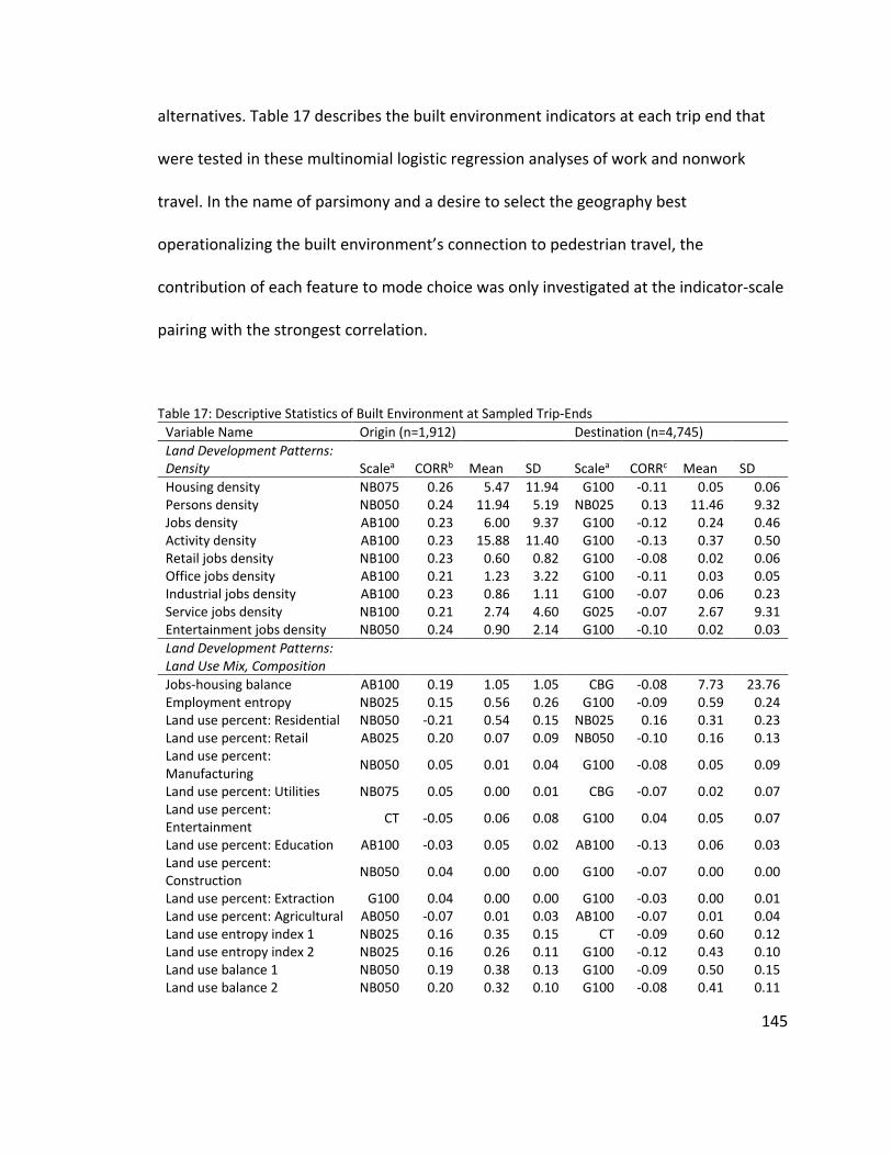
145

alternatives. Table 17 describes the built environment indicators at each trip end that

were tested in these multinomial logistic regression analyses of work and nonwork

travel. In the name of parsimony and a desire to select the geography best

operationalizing the built environment’s connection to pedestrian travel, the

contribution of each feature to mode choice was only investigated at the indicator-scale

pairing with the strongest correlation.

Table 17: Descriptive Statistics of Built Environment at Sampled Trip-Ends

Variable Name Origin (n=1,912) Destination (n=4,745)

Land Development Patterns: Density Scalea CORRb Mean SD Scalea CORRc Mean SD

Housing density NB075 0.26 5.47 11.94 G100 -0.11 0.05 0.06 Persons density NB050 0.24 11.94 5.19 NB025 0.13 11.46 9.32 Jobs density AB100 0.23 6.00 9.37 G100 -0.12 0.24 0.46 Activity density AB100 0.23 15.88 11.40 G100 -0.13 0.37 0.50 Retail jobs density NB100 0.23 0.60 0.82 G100 -0.08 0.02 0.06 Office jobs density AB100 0.21 1.23 3.22 G100 -0.11 0.03 0.05 Industrial jobs density AB100 0.23 0.86 1.11 G100 -0.07 0.06 0.23 Service jobs density NB100 0.21 2.74 4.60 G025 -0.07 2.67 9.31 Entertainment jobs density NB050 0.24 0.90 2.14 G100 -0.10 0.02 0.03

Land Development Patterns: Land Use Mix, Composition

Jobs-housing balance AB100 0.19 1.05 1.05 CBG -0.08 7.73 23.76 Employment entropy NB025 0.15 0.56 0.26 G100 -0.09 0.59 0.24 Land use percent: Residential NB050 -0.21 0.54 0.15 NB025 0.16 0.31 0.23 Land use percent: Retail AB025 0.20 0.07 0.09 NB050 -0.10 0.16 0.13 Land use percent: Manufacturing

NB050 0.05 0.01 0.04 G100 -0.08 0.05 0.09

Land use percent: Utilities NB075 0.05 0.00 0.01 CBG -0.07 0.02 0.07 Land use percent: Entertainment

CT -0.05 0.06 0.08 G100 0.04 0.05 0.07

Land use percent: Education AB100 -0.03 0.05 0.02 AB100 -0.13 0.06 0.03 Land use percent: Construction

NB050 0.04 0.00 0.00 G100 -0.07 0.00 0.00

Land use percent: Extraction G100 0.04 0.00 0.00 G100 -0.03 0.00 0.01 Land use percent: Agricultural AB050 -0.07 0.01 0.03 AB100 -0.07 0.01 0.04 Land use entropy index 1 NB025 0.16 0.35 0.15 CT -0.09 0.60 0.12 Land use entropy index 2 NB025 0.16 0.26 0.11 G100 -0.12 0.43 0.10 Land use balance 1 NB050 0.19 0.38 0.13 G100 -0.09 0.50 0.15 Land use balance 2 NB050 0.20 0.32 0.10 G100 -0.08 0.41 0.11

146


NB025 0.18 0.77 0.14 NB025 0.07 0.82 0.18


NB025 0.18 0.77 0.14 NB025 0.07 0.82 0.17

Land use patches: Residential NB050 -0.19 0.69 0.17 NB025 0.17 0.47 0.27 Land use patches: Retail NB100 0.22 0.22 0.10 NB025 -0.07 0.32 0.21 Land use patches: Manufacturing

AB100 0.10 0.03 0.04 G100 -0.09 0.06 0.09

Land use patches: Utilities CBG -0.04 0.01 0.02 CT -0.09 0.02 0.03 Land use patches: Entertainment

AB075 -0.10 0.02 0.02 AB075 -0.09 0.03 0.03

Land use patches: Education NB050 0.07 0.06 0.04 AB100 -0.16 0.08 0.04 Land use patches: Construction

AB100 -0.09 0.01 0.01 AB100 -0.10 0.01 0.01

Land use patches: Extraction NB050 0.05 0.00 0.00 AB100 -0.06 0.00 0.00 Land use patches: Agricultural CT -0.08 0.01 0.03 AB100 -0.07 0.01 0.02

Land Developments: Land Use Mix, Configuration

Maximum patch size: Residential

NB025 -0.19 0.11 0.11 AB100 -0.11 0.02 0.02

Maximum patch size: Retail G025 0.07 0.03 0.05 AB025 -0.11 0.05 0.08 Maximum patch size: Manufacturing

G100 -0.04 0.01 0.02 AB050 -0.08 0.02 0.04

Maximum patch size: Utilities NB050 0.05 0.00 0.01 CBG -0.06 0.01 0.06 Maximum patch size: Entertainment

AB100 -0.05 0.03 0.04 AB075 0.06 0.02 0.03

Maximum patch size: Education

NB100 -0.09 0.02 0.02 NB100 -0.07 0.02 0.04

Maximum patch size: Construction

G100 -0.05 0.00 0.00 CT -0.08 0.00 0.00

Maximum patch size: Extraction

G100 0.04 0.00 0.00 AB100 -0.03 0.00 0.01

Maximum patch size: Agricultural

AB050 -0.08 0.00 0.02 AB100 -0.07 0.00 0.02

Maximum patch size NB025 -0.18 0.13 0.11 NB025 -0.12 0.16 0.18

Urban Design and Transportation System

Average street block size NB025 -0.16 7.76 7.88 G025 -0.13 10.44 12.40 Alpha index AB100 0.25 0.31 0.10 AB100 0.13 0.33 0.11 Beta index AB100 -0.24 0.63 0.09 AB100 -0.13 0.62 0.09 Cyclomatic index NB050 0.25 96.51 55.98 NB100 0.13 352.95 215.20 Gamma index AB100 0.25 0.54 0.07 AB100 0.13 0.55 0.07 Intersection density AB050 0.21 0.32 0.12 AB075 0.15 0.31 0.13 Intersection proportion CT 0.21 0.86 0.11 AB100 0.16 0.84 0.11 Cul-de-sac density CT -0.18 0.05 0.03 AB100 -0.10 0.05 0.03 Street density NB075 0.22 227.30 51.19 AB075 0.16 204.01 62.03 Percent of local roads NB025 -0.05 0.95 0.09 AB075 0.11 0.89 0.06 Percent of primary roads NB025 0.06 0.01 0.03 CT -0.12 0.04 0.05 Sidewalk coverage CT 0.21 0.69 0.31 AB075 0.14 0.73 0.25

147

Note: a Scale abbreviations: AB025 (areal buffer, 0.25-mile), AB050 (areal buffer, 0.50-mile), AB075 (areal buffer, 0.75-mile), AB100 (areal buffer, 1.00-mile), NB025 (network buffer, 0.25-mile), NB050 (network buffer, 0.50-mile), NB075 (network buffer, 0.75-mile), NB100 (network buffer, 1.00-mile), CBG (Census block group), CT (Census tract), G025 (grid cell, 0.25-mile), G100 (grid cell, 1.00-mile); b Point-biserial correlation with binary variable of household decision to participate in ≥1 walk trip; c Point-biserial correlation with binary variable of individual trip-level decision to walk.

To examine the additive contribution of the built environment on HBW mode

choice, the first step was the estimation of a reduced, base model with alternative-

specific travel time and cost attributes as well as a set of statistically significant

individual-specific attributes (Table 18). This model produced a log-likelihood estimation

of -806.56 and an adjusted McFadden’s R2 value of 0.32. The next steps in this iterative

model building exercise was the forward selection of significant built environment

attributes describing the physical context of the trip origin, followed by a comparable

process to specify significant attributes at the destination. Estimation results of the full

HBW model are provided in Table 19.

Table 18: Base Multinomial Logistic Regression Model Results for Home-Based Work Travel

Travel Mode Alternative a

Public Transit Bicycle Walk

Variable Name B SE B SE B SE

Intercept 2.72 0.69*** -0.95 0.97 5.53 1.03*** Travel Time -0.05 0.01*** -0.01 0.01 -0.12 0.01*** Cost -0.32 0.11**

Individual Characteristics

Gender: Female -0.71 0.19*** 0.43 0.26 -0.34 0.28 Education: Associate’s degree 0.46 0.47 -0.25 0.41 -0.17 0.53 Education: Bachelor’s degree 1.45 0.43*** -0.28 0.39 1.06 0.49* Education: Graduate degree 1.87 0.43*** -0.77 0.43 1.20 0.50* Driver’s license -1.84 0.49*** -1.64 0.46*** -2.41 0.52***

Household Characteristics

Oldest adult: 30 to 44 years old -0.81 0.47 0.40 0.79 -1.05 0.90 Oldest adult: 45 to 64 years old -1.38 0.46** -0.16 0.77 -1.17 0.88 Oldest adult: 65 years or older -2.62 0.62*** -0.32 0.84 -2.07 1.01* Household vehicles per driver -1.72 0.29*** -0.04 0.32 -1.60 0.37***

148

Model Statistics Log-likelihood -806.56 McFadden’s R2 (adjusted) 0.32

Note: a Base alternative = Personal Vehicle; * p < 0.05, ** p < 0.01, *** p < 0.001.

Table 19: Final Multinomial Logistic Regression Model Results for Home-Based Work Travel




Intercept -1.66 1.05 -3.60 1.58* 1.09 1.80 Travel Time -0.04 0.01*** 0.00 0.01 -0.12 0.01*** Cost -0.27 0.12*


Gender: Female -0.71 0.20*** 0.18 0.29 -0.23 0.30 Education: Associate’s degree 0.40 0.50 -0.41 0.45 -0.17 0.57 Education: Bachelor’s degree 1.37 0.46** -0.44 0.43 0.79 0.52 Education: Graduate degree 1.78 0.46*** -1.06 0.49* 0.96 0.54 Driver’s license -2.22 0.52*** -2.72 0.54*** -2.61 0.54***


Oldest adult: 30 to 44 years old -0.91 0.50 0.64 0.88 -1.11 0.98 Oldest adult: 45 to 64 years old -1.25 0.49* -0.46 0.84 -0.97 0.95 Oldest adult: 65 years or older -2.58 0.65*** -0.53 0.93 -1.85 1.09 Household vehicles per driver -1.65 0.31*** -0.49 0.40 -1.34 0.40***

Built Environment (residence)

Housing density 0.11 0.07 -0.16 0.13 0.14 0.08 (Scale: Network Band 0.75-mile) Jobs density -0.12 0.03*** -0.03 0.06 -0.03 0.03 (Scale: Areal Buffer 1.00-mile) Land use balance 2 2.70 0.99** -1.38 1.45 1.26 1.49 (Scale: Network Band 0.50-mile) Alpha index 3.51 1.44* -5.22 2.08* -0.11 3.97 (Scale: Areal Buffer 1.00-mile)

Built Environment (destination)

Housing density 1.05 2.67 7.07 3.00* 16.85 5.20** (Scale: Grid 1.00-mile) Land use percent: Education 8.00 3.90* 18.76 4.24*** -1.54 8.70 (Scale: Areal Buffer 1.00-mile) Land use patches: Entertainment 8.22 2.67** 16.35 3.18*** -0.28 10.06 (Scale: Areal Buffer 0.75-mile) Alpha index 4.73 1.24*** 13.19 1.91*** 7.81 3.93* (Scale: Areal Buffer 1.00-mile)



149

In terms of pedestrian travel for HBW trips, on average, an individual was less

likely to walk than drive or ride as a passenger in a vehicle if he/she possessed a driver’s

license or lived in a household with a higher number of vehicles per licensed driver. As

expected, travel time had a negative relationship with the decision to walk rather than

use a vehicle for work-related travel, while the generic specification of parking cost was

negatively associated with all travel mode alternatives. The decision to bicycle rather

than ride in a vehicle for HBW travel was negatively linked to possessing a driver’s

license or having attained a graduate degree. For home-based trips to work or school,

the decision to choose public transit rather than a vehicle was significantly predicted by

a greater number of individual and household characteristics.

Accounting for select built environment features around the origin and

destination of a HBW trip significantly improved the final model’s fit (𝜒2 = 222.17, p <

0.001). An increase in density of housing units and ratio of observed to possible route

alternatives (alpha index) at the destination had a positive effect on the decision to

select an active mode rather than ride in a private vehicle. An increase in the percentage

of educational land uses and landscape patches related to an entertainment land use

had a positive impact on the decision to bicycle or ride transit when compared to the

base case of auto travel. On average, an individual was more likely to ride transit rather

than in a vehicle if the environment around his/her home was characterized by a

balanced spatial distribution of land uses, increased level of network connectivity, and

lower level of employment density.

150

Fewer built environment features had a significant contribution to the HBNW

choice models; yet, their addition offered a statistically significant expansion (𝜒2 =

103.37, p < 0.001) to the base model (Table 20) which produced a log-likelihood

estimation of -1,037.10 and an adjusted McFadden’s R2 value of 0.40. In the final model

(Table 21), an adult was more likely to walk than ride in a vehicle for nonwork trips if

his/her residential environment had a higher housing unit density or activity-related

complementarity of residential, retail, entertainment, education, and other land uses.

Expectedly, the presence of a large retail landscape patch (e.g., big box store, shopping

mall) at a trip destination was a significant predictor of the decision to use a private

vehicle rather walk for HBNW travel. As with the HBW model, an increase in network

connectivity, signified in the HBNW model by the cyclomatic index, was a significant

determinant in using transit rather than a vehicle.

Table 20: Base Multinomial Logistic Regression Model Results for Home-Based Nonwork Travel




Intercept -3.02 0.73*** -0.18 1.09 2.66 0.45*** Travel Time -0.12 0.01*** -0.12 0.01*** -0.12 0.01*** Cost -0.93 0.13***


Driver’s license -1.51 0.44*** -1.56 1.06 -1.75 0.33*** Bike 3.93 0.54*** -0.26 0.75 0.52 0.14***


Annual income: $25,000 to $49,999 0.10 0.45 0.08 1.20 -0.30 0.27 Annual income: $50,000 to $99,999 -0.02 0.42 -0.31 1.17 -0.40 0.25 Annual income: $100,000 or more 0.10 0.43 -0.24 1.30 -0.51 0.26* Household vehicles per driver -0.86 0.28** -0.29 0.79 -0.64 0.19***

Model Statistics Log-likelihood -1,037.10 McFadden’s R2 (adjusted) 0.40


151

Table 21: Final Multinomial Logistic Regression Model Results for Home-Based Nonwork Travel




Intercept -4.65 1.11*** 5.20 2.76 0.77 0.73 Travel Time -0.11 0.01*** -0.11 0.01*** -0.11 0.01*** Cost -0.90 0.13***


Driver’s license -1.34 0.45** -2.44 1.06* -1.67 0.34*** Bike 3.87 0.54*** -0.07 0.79 0.42 0.15**


Annual income: $25,000 to $49,999 0.15 0.47 0.17 1.16 -0.15 0.28 Annual income: $50,000 to $99,999 0.08 0.43 -0.55 1.18 -0.30 0.26 Annual income: $100,000 or more 0.17 0.44 -1.06 1.43 -0.36 0.27 Household vehicles per driver -0.63 0.27* -0.99 0.95 -0.51 0.20*

Built Environment (residence)

Housing density -0.07 0.06 -0.57 0.28* 0.14 0.04*** (Scale: Network Band 0.75-mile) Activity-related complementarity 2 -1.35 1.07 1.05 2.86 1.63 0.73* (Scale: Network Band 0.25-mile) Land use patches: Retail 5.87 1.69*** -7.92 6.43 -0.32 1.23 (Scale: Network Band 1.00-mile)

Built Environment (destination)

Maximum patch size: Retail 1.76 2.05 -32.97 19.07 -5.88 1.84** (Scale: Areal Buffer 0.25-mile) Cyclomatic index 0.01 0.01*** 0.01 0.01 -0.01 0.00 (Scale: Network Band 0.50-mile)



5.5 Conclusions and Discussion

This study has presented an extensive investigation of the neighborhood effects

of the built environment on travel mode choice that explores the MAUP-related impacts

of scale selection and zonal configuration. Examining variation in the scale extent

chosen to reflect the built environment’s connection to walking, this study found

evidence of scale effects in land development pattern, urban design, and transportation

152

system measures of the built environment. Land use composition indices were affected

by the subjective decision of boundary delineation; exhibiting a stronger association

with walking at a smaller spatial extent. This flattening relationship, which was found at

each trip end and also exhibited by several configuration measures, suggests that

consideration should be given to operationalizing land use mix at a disaggregate scale in

studies of pedestrian travel. By adding complexity in land use composition and

configuration, the feasibility of walking is improved by bringing residential and non-

residential activities in closer proximity.

However, inconsistencies with this trend were revealed when operationalizing

certain density and network connectivity indices at greater levels of aggregation. In

general, these measures, when observed at the origin, displayed a stronger association

with walking as the spatial scale increased. This discrepancy highlights a prospect that

different extents or zoning schemes may be more suitable when measuring the various

contextual influences of pedestrian travel and that a more aggregate spatial extent may

be sufficient in assessing this connection for connectivity or density measures. Zoning

effects, which are likely more meaningful when using fixed scale zonal systems, were

also suggested to influence sliding scale neighborhood representations and must be

considered when operationalizing the built environment determinants of active and

passive modes of travel. Provided these and other trends of this MAUP-related analysis,

the following suggestions regarding geographic boundary selection may prove useful for

future research into the built environment determinants of walking:

153

• Sliding geographic scales should be adopted for built environment measurement

whenever possible,

• Measurement near origin should be prioritized but will not provide a complete

picture of the trip’s physical context, and

• Consider operationalizing land use mix measures at a more disaggregate spatial

extent than other built environment indicators.

A second study component was the examination of neighborhood effects of the

built environment at each trip end on mode choice at the home location for work and

nonwork travel. Having identified the combination of indicator and geography

producing the strongest association with walking, model results found the physical

context near each trip end significantly explained mode choice for both trip purposes.

Built environment features at an individual’s work or school location appeared to

explain more variation in home-based travel mode choice than his/her residential

environment, while the context surrounding the home location had a seemingly

stronger role on modal decisions for nonwork travel. Expectedly, the role of the built

environment was less impactful on nonwork travel, which includes discretionary trips

for recreational or social activities that are typically not routine. However, as supported

in the transportation and public health literature (e.g., Brownson, et al., 2009; Ewing &

Cervero, 2010), land development pattern, urban design, and transportation system

characteristics mattered in the decision to perform work or nonwork travel via a more

154

sustainable transportation mode. In general, individuals who chose walking rather

driving or riding in a private vehicle to conduct work-related travel were influenced by

residential density and network connectivity at the trip end; whereas, land development

patterns around each trip end had the greatest effect on the decision to walk for

nonwork trips.

Findings from this study’s MAUP-related and mode choice analyses have

important implications for transportation-land use planning research. First, greater

deliberation should be given to the decision of geographic boundary selection when

operationalizing built environment features. As demonstrated, an increase in geographic

scale extent can produce an amplified or waning importance for certain contextual

determinants of active travel. Relatedly, the neighborhood effect of the built

environment should not be simply standardized using one spatial extent or zoning

system when investigating the impact of different built environment dimensions on

travel. By using disaggregate data and testing the sensitivity of applying different levels

of aggregation, researchers can better identify the spatial boundaries at which

contextual factors exert their actual or strongest influence on the individual behaviors

being studied (Kwan, 2012). In this study, the specification of built environment

indicators operationalized based on the strength of their association to walking

emphasized the significance of isolating the physical context at each trip end on an

individual’s choice of travel mode. Since most transportation decisions are context-

dependent, studies of the transportation-land use connection must clearly distinguish

155

the role of the built environment at each trip end on travel decisions for work and

nonwork activities. By doing so, researchers can help to better guide land use policies

and programs aimed at facilitating walking for transportation and physical activity.

Future efforts should extend this study’s contributions, both conceptually and

methodologically. First, the contextual features in the mode choice models were

operationalized based on associations with walking; however, the appropriate spatial

extent for studying this transportation-land use connection is likely to vary with travel

speed. Pedestrians, who travel at slower speeds, have a greater ability to process the

complexity of their immediate setting, so a suitable scale to measure the neighborhood

effect of the built environment on walking is expected to be smaller than users of faster

modes (Frank & Engelke, 2001). Second, a complete depiction of a traveler’s context

should consider the dual characterization of the built environment at local and regional

levels (Handy, 1992). One study extension would be to model the built environment

connection to mode choice by concurrently testing the auto-centric and pedestrian-

oriented spatial extents of the same indicator. Third, the phenomenon of residential

self-selection warrants further attention in the mode choice analysis since decisions

involving residential neighborhood and, to a lesser extent, workplace location may have

a confounding role in the mode used to perform HBW travel. Finally, given that travel

time was a significant deterrent to walking for both work and nonwork trips, an exciting

contribution to the evidence base would be an inspection of the scaling and zoning

effects of the built environment’s connection to destination choice for pedestrian travel

156

(e.g., Clifton, et al., 2016). Yet, despite these limitations and prospects for future study,

this work in its present state provides a systematic assessment of the impact of

geographic scale choice on understanding the complex interactions between the built

environment and travel behavior.

157

Chapter 6: Conclusions

This dissertation introduced an improved conceptualization and measurement of

land use mix and then systematically explored its connection to pedestrian travel in a

comprehensive, behavioral framework. In doing so, this collection of studies addressed

the three research questions stated in the introduction. This concluding chapter begins

by summarizing the overarching contributions of this collective work and the findings

from each of the three studies as they relate to the research question they addressed. A

depiction of the potential implications of this work for transportation planning practice

follows. The chapter then details the main limitations of the adopted research design

and concludes by describing a set of exciting directions for future research into the topic

of land use mix and pedestrian travel behavior.

6.1 Contributions and Findings

The increased availability of disaggregate land use data has resulted in the wide

adoption of an array of built environment indicators in recent studies of pedestrian

travel behavior. While potentially informative and helpful in building an evidence base,

the selection of ad hoc environmental measures without a strong theoretical connection

to anticipated behavioral responses can also create negative connotations for properly

understanding the interactions between the built environment and pedestrian travel

behaviors. By deconstructing land use mix and reimagining this multifaceted construct

158

as a collection of complementary landscape pattern metrics, this dissertation provides

important theoretical and empirical contributions for transportation-land use planning

research and practice.

Despite a demonstrated interest in linking land use mix to pedestrian travel, a

conceptually valid land use mix measure that yields more consistent and generalizable

results is missing from planning research (Song, et al., 2013). Land use entropy, which is

a commonly adopted pattern measure of land use mix, originated in information

sciences and has no theoretical basis as an indicator of pedestrian travel behavior.

Consequently, the assumption of compositional evenness and inattention to land use

complementarity or spatial configuration, which are intrinsic to any land use entropy

measure, hinder its ability to adequately inform transportation-land use policy. In

response, this dissertation combined activity-based travel behavior and landscape

ecology theory to introduce a land use mix measure that explicitly accounts for how the

spatial configuration of local land uses may also facilitate increased pedestrian travel.

Beyond offering a conceptual advancement, the application of this multifaceted

land use mix construct in this dissertation represented an achievement toward meeting

a transportation-land use planning goal to find mix indicators that more accurately and

efficiently measure its influence on particular travel outcomes (Manaugh & Krieder,

2013). The activity-related complementarity measure provides an indication of what

land use composition mirrors derived travel demand, which planners may then use to

infer the land use type most needed in a neighborhood to improve its walkability. This

159

insight cannot be obtained from present mix indicators and may prove valuable in the

development of area plans or performance-based zoning standards seeking to increase

the feasibility of pedestrian travel in a neighborhood. In all, by placing greater attention

to the composition and configuration of land use types as well as the boundary chosen

to delineate the impact of these complementary pattern aspects, planning researchers

can begin to better apprise planning practitioners of the pedestrian travel impacts of

certain land use compositions and configurations within a neighborhood.

The study described in Chapter 3 investigated the relationship between

pedestrian travel and land use mix when considering the complementarity, composition,

and configuration of local land use types. A persistent limitation in past studies of this

transportation-land use connection has been an absence in the explicit consideration of

the spatial arrangement of land use types in the measurement of land use mix. In

response, this study introduced a land use mix construct reflected by indicators of land

use composition as well as the corresponding pattern aspect of spatial configuration. A

second contribution of this study was the development of an activity-related

complementarity measure that explains an ideal composition of land uses based on

derived travel demand rather than spatial equilibrium. This activity-related indicator can

redirect the quantification of land use diversity away from the athoeretical equal

balance assumption, which is intrinsic to the commonly used entropy index, and toward

activity complementarity. Application of a confirmatory factor analysis framework

provided a hypothesis-driven process for identifying a land use mix construct reflective

160

of two composition, including this activity-related complementarity measure, and two

configuration indicators. The land use mix construct was a stronger predictor of walk

mode choice than land use entropy and a significant determinant of home-based walk

trip frequency when accounting for other common built environment covariates.

A second empirical study, described in Chapter 4, examined the impact of land

use mix and other smart growth features on pedestrian travel for transportation-related

and discretionary trip purposes. While past research has examined these relationships,

these studies largely depict the built environment as a series of isolated measures

rather than as a bundle of synergistic indicators and inadequately account for the

indirect effects of the various explanatory factors influencing one another and

pedestrian travel. A primary study contribution was the identification of a second-order

factor that described a smart growth neighborhood comprising the three interrelated

tenets of land use mix, employment concentration, and pedestrian-oriented design. A

structural equation modeling strategy was then used to examine the impact of this

multidimensional conceptualization of the built environment on pedestrian travel as

portrayed in a proposed multidirectional conceptual model. The study was novel in its

adoption of this advanced analytic strategy to link multiple latent constructs reflected

by objective indicators to pedestrian travel behaviors. Findings revealed that residing

within a smart growth neighborhood was a strong, positive predictor of the household-

level decision to participate in at least one walk trip for transportation or discretionary

purposes. Accordingly, this study provided planners an identified set of indicators that

161

may be toggled to improve built environment efficiencies and encourage physically

active modes of travel within local neighborhoods.

Chapter 5 delivered a final empirical study that explored the influence of

operationalizing land use mix and other built environment features at varying

geographic scales on their hypothesized connections to individual travel behavior. The

likelihood of scale-related decisions to distort the significance or degree of these

relationships has likely confounded findings from past studies examining how the

physical context near each trip end effects an individual’s travel behavior for different

trip purposes. This study contributed to a limited evidence base investigating the scale

and zoning effects of understanding the impact of land development pattern, urban

design, and transportation system features on pedestrian travel at different geographic

boundaries. A result of this descriptive sensitivity analysis was a recognition of the

pairing of scale and built environment indicator that produced the strongest association

with pedestrian travel at each trip end. While not definitive, this effort provided insight

into the boundary at which certain physical context features exert their genuine

influence on walking behaviors. By using discrete choice analysis, a second study

contribution involved the modeling of home-based travel for work and nonwork

activities as a function of personal, household, and trip characteristics as well as this

context at each trip end. Few studies in the literature have assessed mode choice for

different trip purposes with such an extensive set of objective measures to understand

the role of land use at the trip origin and destination. Findings from this effort found

162

that development patterns, designated by land use mix and density measures, at each

trip end had a strong effect on the decision to walk rather than use a private vehicle for

nonwork trips.

6.2 Practical Implications

Beyond these scholarly contributions, this dissertation also has several practical

implications for transportation planners interested in pedestrian travel. First, extending

the theoretical conceptualization of land use mix can help to inform smart growth and

infill development plans as to the proper balance of activity locations needed to achieve

neighborhood-level walkability. Present indicators of land use mix are insufficient

performance measures due to imperfect theoretical foundations, inconsistent findings,

and a general mismatch between measurement and intended outcome. The activity-

related complementarity measure offers planners an alternative composition measure

to the entropy index that defines local land use mix based on the distribution of activity

locations that generate observed travel demand. Therefore, a neighborhood

characterized by an activity-related distribution of land uses could enable individuals to

walk to the types of destinations that derive their need for travel. While more research

is needed, findings from each study revealed a consistently positive relationship

between this new mix metric and walking. If this trend holds true in other contexts, then

transportation planners will have greater insight into the ideal balance of land uses

needed to facilitate higher levels of physical activity.

163

Second, the positive association revealed between walking and neighborhoods

with land use mix, employment concentration, and pedestrian-oriented design can

redirect urban development discussions away from contentious debates focused on

residential densification. The first study found that local land use mixing defined by

complexity in both composition and configuration, and not population density, was a

strong predictor of home-based walk trip frequency. In the next empirical study, the

multidimensional construct of a smart growth neighborhood, which was not informed

by population density, had a strong direct and total effect on home-based walking for

both transportation-related and discretionary purposes. This latter study showed that

local land use mixing may be combined with other smart growth principles to create a

walkable environment where increased levels of walking are observed. Aside from a

focus on upzoning residential land uses to allow for greater density, planners should

seek alternative options (e.g., rezoning) that permit the integration of local retail stores

within predominately residential neighborhoods.

Lastly, transportation planners and engineers must be cognizant that geographic

scale selection influences the study of spatial-dependent behaviors. While this notion is

implicit in transportation-land use study and practice, few previous efforts have

systematically investigated the sensitivity of contextual measures and their association

with walking through spatial scale variation. Planners should give greater consideration

to the spatial boundaries at which contextual factors exert their actual influence and

subsequently how they operationalize built environment measures to understand their

164

connection to travel behavior. Misconceptions of the built environment can result in

measurement error and an inaccurate reflection of how pedestrian travel behaviors are

affected by changes to the current land development patterns, urban design features,

and transportation systems found within neighborhoods.

6.3 Limitations

This section briefly summarizes two major limitations of this dissertation

research. The examination of interactions between the built environment and travel

behavior with longitudinal data and an unravelling of the influence of residential self-

selection on these connections are areas of research left unfulfilled by this dissertation.

Travel behavior data analyzed in this research were cross-sectional, which inhibited the

ability to confidently claim that built environment modifications seeking to improve

neighborhood-level land use mixing caused increases in pedestrian travel. This research

found that land use mix had a strong, positive association with walking, but no

directionality regarding that association can be established. While use of structural

equation modeling enabled the testing of bidirectional relationships outlined in the

conceptual model, any analysis of cross-sectional data does not provide the condition of

time precedence needed to establish this missing causal link.

Relatedly, this research did not explicitly account for any potential statistical bias

to model results produced by residential self-selection. Household decisions of where to

reside may be manifestations of the travel preferences of its members. Accordingly, an

165

individual who is predisposed to more active modes of travel may choose to reside in

smart growth neighborhoods; therefore, increases in the land use mixing may be less of

a determining factor of walking than residential sorting. Although this idea of residential

self-selection can be accounted for within cross-sectional data (i.e., use of psychosocial

measures), the importance of this phenomenon in transportation-land use studies is

likely best captured via longitudinal analyses.

6.4 Future Directions

This dissertation concludes with a look to the future by identifying areas where

this work can be extended. In Chapter 2, three land use mix components were

identified: land use interaction, geographic scale, and temporal availability. While

empirical advancements to the first two components were made in this dissertation, the

opportunity to access land use types at a specific time was not quantified. Future efforts

should explore to what extent, if any, the inclusion of temporal availability in land use

mix indicators better explains travel behavior variation than conventional mix measures.

Introducing the temporal availability component, which is missing from the present land

use mix measures that have portrayed a timeless illustration of the diversity in activity

opportunity supply, would progress this dissertation work. In theory, the adoption of a

time-based land use mix measure can help support innovative transportation-land use

policies, identify social inequities in distance-based accessibility, and improve behavioral

models of travel demand.

166

To ease the transferability of this research to practice, the land use mix construct

introduced in Chapter 3 could be reimagined as an index based on the four identified

indictors. Alternatively, a new land use mix indicator that is expressed as a mathematical

formulation combining the proposed activity-related complementarity measure with the

contagion index could be explored. A theoretically grounded measure that encompasses

both composition and configuration aspects will better guide existing transportation-

land use policies by identifying thresholds of land use mix that are needed to achieve

higher levels of active travel and physical activity.

Another dissertation extension would be to add complexity to the analytic

framework presented in Chapter 4 by incorporating individual-level psychosocial

measures and pedestrian travel outcomes to improve the depiction of mechanisms

outlined in the conceptual model. While perceptions of the built environment are

subject to reporting bias and more difficult to translate into practice, these psychosocial

measures offer valuable insight and their absence in this work likely confounds the

reported findings. In addition, the application of a hierarchical modeling framework

would enable individual-level walking behaviors to be analyzed. As it stands, this study

linked walkability at the home location to the household-level decision to participate in

at least one walk trip, a theoretically imperfect strategy for operationalizing walking. By

including individual-level psychosocial measures and walking behaviors, future efforts

can provide a more robust understanding of the relative impact of land use mix and

167

other smart growth factors, which are established transportation planning tools, for

increasing pedestrian activity.

Finally, the operationalization of land use mix as well as density, urban design,

and transportation system measures with perceptive geographic scales should be

sought after. In the final study, the use of network bands to capture the neighborhood

effects of the built environment objectively limited the area considered by an individual

to affect travel based on access to the street network. However, a subjective quality of

the built environment related to an individual’s perception of what may be physically

reached is a more theoretically justifiable way to delineate a neighborhood and define

what features impact travel. A recognition of these cognitive confinements of individual

movement to nearby activity locations will further refine the ability to understand how

local land use mixing affects pedestrian travel behavior.

168

References Aditjandra, P., Cao, X., & Mullet, C. (2012). Understanding neighbourhood design impact

on travel behavior: An application of structural equations model to a British metropolitan data. Transportation Research Part A, 46, 22-32.

Aditjandra, P.T., Mulley, C. (2016). Exploring changes in public transport use and walking following residential relocation: A British case study. The Journal of Transport and Land Use, 9(3), 1-19.

Anderson, J., & Gerbing, D. (1988). Structural equation modeling in practice: A review and recommended two-step approach. Psychological Bulletin, 103(4), 411-423.

Arentze, T., & Timmermans, H. (2005). Representing mental maps and cognitive learning in micro-simulation models of activity-travel choice dynamics. Transportation, 32, 321-340.

Badoe, D., & Miller, E. (2000). Transportation-land use interaction: Empirical findings in North America, and their implications for modeling. Transportation Research Part D, 5(4), 235-263.

Bagley, M., & Mokhtarian, P. (2002). The impact of residential neighborhood type on travel behavior: A structural equations modeling approach. The Annals of Regional Science, 36, 279-297.

Bagley, M.N., Mokhtarian, P.L., & Kitamura, R. (2002). A methodology for the disaggregate, multidimensional measurement of residential neighbourhood type. Urban Studies, 39, 4, 689-704.

Banerjee, U., & Hine, J. (2016). Interpreting the influence of urban form on household car travel using partial least squares structural equation modelling: Some evidence from Northern Ireland. Transportation Planning and Technology, 39(1), 24-44.

Ben-Akiva, M., & Lerman, S. (1985). Discrete choice analysis: Theory and application to travel demand. Cambridge, MA: The Massachusetts Institute of Technology Press.

Berke, E.M., Koepsell, T.D., Moudon, A.V., Hoskins, R.E., & Larson, E.B. (2007). Association of the built environment with physical activity and obesity in older persons. American Journal of Public Health, 97(3), 486-492.

Bhat, C., & Gossen, R. (2004). A mixed multinomial logit model analysis of weekend recreational episode type choice. Transportation Research Part B, 38, 767-787.

Boarnet, M. (2011). A broader context for land use and travel behavior, and a research agenda. Journal of the American Planning Association, 77(3), 197-213.

Boarnet, M., & Sarmiento, S. (1998). Can land-use policy really affect travel behavior? A study of the link between nonwork travel and land-use characteristics. Urban Studies, 35(7), 1155-1169.

Boarnet MG, Joh K, Siembab W, Fulton W and Nguyen MT (2011) Retrofitting the suburbs to increase walking: Evidence from a land-use-travel study. Urban Studies, 48(1), 129-159.

169

Boer, R., Zheng, Y., Overton, A., Ridgeway, G., & Cohen, D. (2007). Neighborhood design and walking trips in ten U.S. metropolitan regions. American Journal of Preventive Medicine, 32(4), 298-304.

Boone-Heinonen, J., Popkin, B.M., Song, Y., & Gordon-Larsen, P. (2010). What neighborhood area captures built environment features related to adolescent physical activity? Health & Place, 16, 1280-1286.

Brown, B., Yamada, I., Smith, K., Zick, C., Kowaleski-Jones, L., & Fan, J. (2009). Mixed land use and walkability: Variations in land use measures and relationships with BMI, overweight, and obesity. Health & Place, 15, 1130-1141.

Brown, T. (2006). Confirmatory factor analysis for applied research. New York, NY: The Guilford Press.

Brownson, R., Hoehner, C., Day, K., Forsyth, A., & Sallis, J. (2009). Measuring the built environment for physical activity: State of the science. American Journal of Preventive Medicine, 36(4), S99-S123.e12.

Buehler, R. (2011). Determinants of transport mode choice: A comparison of Germany and the USA. Journal of Transport Geography, 19, 644-657.

Burns, L. (1979). Transportation, temporal, and spatial components of accessibility. Lexington, MA: D.C. Heath and Company.

Cao, X. (2015). Examining the impacts of neighborhood design and residential self-selection on active travel: A methodological assessment. Urban Geography, 36(2), 236-255.

Cao, X. (2016). How does neighborhood design affect life satisfaction? Evidence from Twin Cities. Travel Behaviour and Society, 5, 68-76.

Cao, X., & Chatman, D. (2016). How will smart growth land-use policies affect travel? A theoretical discussion on the importance of residential sorting. Environment and Planning B: Planning and Design, 43, 58-73.

Cao, X., Handy, S.L., & Mokhtarian, P.L. (2006). The influence of the built environment and residential self-selection on pedestrian behavior: Evidence from Austin, TX. Transportation, 33, 1-20.

Cao, X., Mokhtarian, P.L., & Handy, S.L. (2007). Do changes in neighborhood characteristics lead to changes in travel behavior? A structural equations modeling approach. Transportation, 34, 535-556.

Cerin, E., Leslie, E., du Toit, L., Owen, N., & Frank, L. (2007). Destinations that matter: Associations with walking for transport. Health & Place, 13, 713-724.

Cervero, R. (1988). Land-use mixing and suburban mobility. Transportation Quarterly, 42(3), 429-446.

Cervero R. (1989). Suburban employment centers: Probing the influence of site features on the journey-to-work. Journal of Planning Education and Research, 8(2), 75-85.

Cervero R. (1996). Mixed land-uses and commuting: Evidence from the American Housing Survey. Transportation Research Part A, 30(5), 361-377.

Cervero, R. (2002). Built environments and mode choice: Toward a normative framework. Transportation Research Part D, 7, 265-284.

170

Cervero, R., & Duncan, M. (2003). Walking, bicycling, and urban landscapes: Evidence from the San Francisco Bay Area. American Journal of Public Health, 93(9), 1478-1483.

Cervero, R., & Kockelman, K. (1997). Travel demand and the 3Ds: Density, diversity, and design. Transportation Research Part D, 2(3), 199-219.

Cervero, R., & Radisch, C. (1996). Travel choices in pedestrian versus automobile oriented neighborhoods. Transport Policy, 3(3), 127-141.

Chen, Y., Ravulaparthy, S., Deutsch, K., Dalal, P., Yoon, S. Y., Lei, T., Goulias, K., Pendyala, R., Bhat, C., & Hu, H. (2011). Development of indicators of opportunity-based accessibility. Transportation Research Record: Journal of the Transportation Research Board, 2255, 58-68.

Christian, H., Bull, F., Middleton, N., Knuiman, M., Divitni, M., Hooper, P., Amarasinghe, A., & Giles-Corti, B. (2011). How important is the land use mix measure in understanding walking behavior? Results from the RESIDE study. International Journal of Behavioural Nutrition and Physical Activity, 8, 55-67.

Clark, A., & Scott, D. (2014). Understanding the impact of the modifiable areal unit problem on the relationship between active travel and the built environment. Urban Studies, 51(2), 284-299.

Clifton, K., Ewing, R., Knaap, G., & Song, Y. (2008). Quantitative analysis of urban form: A multidisciplinary review. Journal of Urbanism: International Research on Placemaking and Urban Sustainability, 1(1), 17-45.

Clifton, K.J., Livi Smith, A.D., & Rodriguez, D.A. (2007). The development and testing of an audit for the pedestrian environment. Landscape and Urban Planning, 80, 95-110.

Clifton, K.J., Singleton, P.A., Muhs, C.D., & Schneider, R.J. (2016). Development of destination choice models for pedestrian travel. Transportation Research Part A: Policy and Practice, 94, 255-265.

Crane, R. (1996). On form versus function: Will the new urbanism reduce traffic, or increase it? Journal of Planning Education and Research, 15, 117-126.

Crane, R. (2000). The influence of urban form on travel: An interpretive review. Journal of Planning Literature, 15(3), 3-23.

de Abreu e Silva, J., Golub, T.F., & Goulias, K.G. (2006). Effects of land use characteristics on residence and employment location and travel behavior of urban adult workers. Transportation Research Record: Journal of the Transportation Research Board, 1977, 121-131.

de Abreu e Silva, J., & Goulias, K.G. (2009). Structural equations model of land use patterns, location choice, and travel behavior: Seattle, Washington compared with Lisbon, Portugal. Transportation Research Record: Journal of the Transportation Research Board, 2135, 106-113.

de Abreu e Silva, J., Goulias, K.G., & Dalal, P. (2012a). Structural equations model of land use patterns, location choice, and travel behavior in Southern California. Transportation Research Record: Journal of the Transportation Research Board, 2323, 35-45.

171

de Abreu e Silva, J., Morency, C., & Goulias, K. (2012b). Using structural equation modeling to unravel the influence of land use patterns on travel behavior of workers in Montreal. Transportation Research Part A, 46, 1252-1264.

de Winter, J.C.F., & Dodou, D. 2012. Factor recovery by principal axis factoring and maximum likelihood factor analysis as a function of factor pattern and sample size. Journal of Applied Statistics, 39(4), 695-710.

Deutsch, K., Yoon, S.Y., & Goulias, K. (2013). Modeling travel behavior and sense of place using a structural equation model. Journal of Transport Geography, 28, 155-163.

Delafontaine, M., Neutens, T., Schwanen, T., & Van de Weghe. (2011). The impact of opening hours on the equity of individual space-time accessibility. Computers, Environment, and Urban Systems, 35, 276-288.

Dill, J. Measuring network connectivity for bicycling and walking. Presented at 83rd Annual Meeting of the Transportation Research Board, Washington (2004)

Downs, A. (2005). Smart growth: Why we discuss it more than we do it. Journal of the American Planning Association, 71(4), 367-378.

Duncan, M., Winkler, E., Sugiyama, T., Cerin, E., du Toit, L., Leslie, E., & Owen, N. (2010). Relationships of land use mix with walking for transport: Do land uses and geographical scale matter? Journal of Urban Health: Bulletin of the New York Academy of Medicine, 87(5), 782-795.

Eboli, L., Forciniti, C., & Mazzulla, G. (2012). Exploring land use and transport interaction through structural equation modeling. Procedia Social and Behavioral Sciences, 54, 107-116.

Ewing, R., & Cervero, R. (2001). Travel and the built environment: A synthesis. Transportation Research Record: Journal of the Transportation Research Board, 1780, 87-114.

Ewing, R., & Cervero, R. (2010). Travel and the built environment: A meta-analysis. Journal of the American Planning Association, 76(3), 265-294.

Ewing, R., Pendall, R., & Chen, D. (2003). Measuring sprawl and its transportation impacts. Transportation Research Record: Journal of the Transportation Research Board, 1831, 175-183.

Ewing, R., Schroeer, W., & Greene, W. (2004). School location and school travel: Analysis of factors affecting mode choice. Transportation Research Record: Journal of the Transportation Research Board, 1895, 55-63.

Ewing, R., Tian, G., Goates, J., Zhang, M., Greenwald, M.J., Joyce, A., Kircher, J., & Greene, W. (2015). Varying influences of the built environment on household travel in 15 diverse regions of the United States. Urban Studies, 52(13), 2330-2348.

Fan, Y., & Khattak, A. (2008). Urban form, individual spatial footprints, and travel: Examination of space-use behavior. Transportation Research Record: Journal of the Transportation Research Board, 2082, 98-106.

Ford, J.K., MacCallum, R.C, & Tait, M. (1986). The application of exploratory factor analysis in applied psychology: A critical review and analysis. Personnel Psychology, 39, 291-314.

172

Forsyth, A., Hearst, M., Oakes, J., & Schmitz, K. (2008). Design and destination: Factors influencing walking and total physical activity. Urban Studies, 45(9), 1973-1996.

Fotheringham, A., & Wong, D. (1991). The modifiable areal unit problem in multivariate statistical analyses. Environment and Planning A, 23, 1025-1044.

Frank, L.D. (2000) Land use and transportation interaction: Implications on public health and quality of life. Journal of Planning Education and Research, 20, 6-22.

Frank L.D., Andresen, M.A., & Schmid, T.L. (2004). Obesity relationships with community design, physical activity, and time spent in cars. American Journal of Preventive Medicine, 27(2), 87-96.

Frank, L., Bradley, M., Kavage, S., Chapman, J., & Lawton, T. (2008). Urban form, travel time, and cost relationships with tour complexity and mode choice. Transportation, 35, 37-54.

Frank, L., & Engelke, P. (2001). The built environment and human activity patterns: Exploring the impact of urban form on public health. Journal of Planning Literature, 16, 202-218.

Frank, L., & Kavage, S. (2009). A national plan for physical activity: The enabling role of the built environment. Journal of Physical Activity and Health, 6(2), S186-S195.

Frank, L., Kerr, J., Chapman, J., & Sallis, J. (2007). Urban form relationships with walk trip frequency and distance among youth. American Journal of Health Promotion, 21(4), 305-311.

Frank, L., & Pivo, G. (1994). Impacts of mixed use and density on utilization of three modes of travel: Single-occupant vehicle, transit, and walking. Transportation Research Record: Journal of the Transportation Research Board, 1466, 44-52.

Frank, L., Schmid, T., Sallis, J., & Chapman, J. (2005). Linking objectively measured physical activity with objectively measured urban form: Findings from SMARTRAQ. American Journal of Preventive Medicine, 28(2S2), 117-125.

Gauvin, L., Robitaille, E., Rive, M., McLaren, L., Dassa, C., & Potvin. L. (2007). Conceptualizing and operationalizing neighbourhoods: The conundrum of identifying territorial units. Canadian Journal of Public Health, 98(1), S18-S26.

Gehlke, C.E., & Biehl, K. (1934). Certain effects of grouping upon the size of the correlation coefficient in census tract material. Journal of the American Statistical Association, 29(185), 169-170.

Gehrke, S.R., & Clifton, K.J. (2014). Operationalizing land use diversity at varying geographic scales and its connection to mode choice: Evidence from Portland, Oregon. Transportation Research Record: Journal of the Transportation Research Board, 2453, 128-136.

Gehrke, S.R., & Clifton, K.J. (2016). Toward a spatial-temporal measure of land-use mix. The Journal of Transport and Land Use, 9(1), 171-186.

Gehrke, S.R., & Clifton, K.J. (2017a). An activity-related land use mix construct and its connection to pedestrian travel. Environment & Planning B: Urban Analytics and City Science, Forthcoming.

173

Gehrke, S.R., & Clifton, K.J. (2017b). A pathway linking smart growth neighborhoods to home-based pedestrian travel. Travel Behaviour and Society, 7, 52-62.

Geurs, K., & van Wee, B. (2004). Accessibility evaluation of land-use and transport strategies: Review and research directions. Journal of Transport Geography, 12, 127-140.

Golob, T. (2003). Review: Structural equation modeling for travel behavior research. Transportation Research Part B, 37, 1-25.

Goodchild, M., & Janelle, D. (1984). The city around the clock: space-time patterns of urban ecological structure. Environment and Planning A, 16, 807-820.

Grant, J. (2002). Mixed use in theory and practice: Canadian experience with implementing a planning principle. Journal of the American Planning Association, 68(1), 71-84.

Guo, J., & Bhat, C. (2007). Operationalizing the concept of neighborhood: Application to residential location choice analysis. Journal of Transport Geography, 15, 31-45.

Gustafson, E. (1998). Quantifying landscape spatial pattern: What is the state of the art? Ecosystems, 1, 143-156.

Hagerstrand, T. (1970). What about people in regional science? Papers in Regional Science, 24(1), 6-21.

Handy, S. (1993). Regional versus local accessibility: Implications for nonwork travel. Transportation Research Record: Journal of the Transportation Research Board, 1400, 58-66.

Handy, S. (2005). Smart growth and the transportation-land use connection: What does the research tell us? International Regional Science Review, 28(2), 146-167.

Handy, S., Boarnet, M., Ewing, R., & Killingsworth, R. (2002). How the built environment effects physical activity: View from urban planning. American Journal of Preventive Medicine, 23(2S), 64-73.

Handy, S., Cao, X., & Mokhtarian, P. (2006). Self-selection in the relationship between the built environment and walking: Empirical evidence from Northern California. Journal of the American Planning Association, 72(1), 55-74.

Handy, S.L., & Clifton, K.J. (2001). Local shopping as a strategy for reducing automobile travel. Transportation, 28, 317-346.

Handy, S., & Niemeier, D. (1997). Measuring accessibility: An exploration of issues and alternatives. Environment & Planning A, 29, 1175-1194.

Hansen, W. (1959). How accessibility shapes land use. Journal of the American Institute of Planners, 25(2), 73-76.

Hanson, S. (1980). The importance of the multi-purpose journey to work in urban travel behavior. Transportation, 9, 229-248.

Hayton, J.C., Allen, D.G., & Scarpello, V. (2004). Factor retention decisions in exploratory factor analysis: A tutorial on parallel analysis. Organizational Research Methods, 7(2), 191-205.

174

Hess, P., Moudon, A., & Logsdon, M. (2001). Measuring land use patterns for transportation research. Transportation Research Record: Journal of the Transportation Research Board, 1780, 17-24.

Hoehner, C.M., Brennan Ramirez, L.K., Elliott, M.B., Handy, S.L., & Brownson, R.L. (2005). Perceived and objective environmental measures and physical activity among urban adults. American Journal of Preventive Medicine, 28(2S2), 105-116.

Hong, J., Shen, Q., & Zhang, L. (2013). How do built-environment factors affect travel behavior? A spatial analysis at different geographic scales. Transportation, 41, 419-440.

Horner, M., & Murray, A. (2002). Excess commuting and the modifiable areal unit problem. Urban Studies, 39(1), 131-139.

Horton, F., & Reynolds, D. (1971). Effects of urban spatial structure on individual behavior. Economic Geography, 47(1), 36-48.

Houston, D. (2014). Implications of the modifiable areal unit problem for assessing built environment correlates of moderate and vigorous physical activity. Applied Geography, 50, 40-47.

Jelinski, D.E., & Wu, J. (1996). The modifiable areal unit problem and implications for landscape ecology. Landscape Ecology, 11(3), 129-140.

Kerr, J., Frank, L., Sallis, J.F., & Chapman, J. (2007). Urban form correlates of pedestrian travel in youth: Differences by gender, race-ethnicity and household attributes. Transportation Research Part D, 12, 117-182.

Kerr, J., Norman, G., Millstein, R., Adams, M.A., Morgan, C., Langer, R.D., & Allsion, M. (2014). Neighborhood environment and physical activity among older women: Findings from the San Diego cohort of the women’s health initiative. Journal of Physical Activity & Health, 11, 1070-1077.

Kerr, J., Rosenberg, D., Sallis, J., Saelens, B., Frank, L. & Conway, T. (2006). Active commuting to school: Associations with environment and parental concerns. Official Journal of the American College of Sports Medicine, 38(4), 787-794.

Kim, H., & Kwan, M. P. (2003). Space-time accessibility measure: A geocomputational algorithm with a focus on the feasible opportunity set and possible activity duration. Journal of Geographical Systems, 5, 71-91.

Kitamura, R., Mokhtarian, P., & Laidet, L. (1997). A micro-analysis of land use in five neighborhoods in the San Francisco Bay Area. Transportation, 24, 125-158.

Kitamura, R., Akiyama, T., Yamamoto, T., & Golob, T. (2001). Accessibility in a metropolis: Toward a better understanding of land use and travel. Transportation Research Record: Journal of the Transportation Research Board, 1780, 64-75.

Kockelman, K. (1997). Travel behavior as function of accessibility, land use mixing, and land use balance: Evidence from San Francisco Bay Area. Transportation Research Record: Journal of the Transportation Research Board, 1607, 116-125.

Koppelman, F., & Bhat, C. (2006). A self-instructing course in model choice modeling: Multinomial and nested logit models. Washington, DC: United States Department of Transportation, Federal Transit Administration.

175

Krizek, K. (2003a). Residential relocation and changes in urban travel: Does neighborhood-scale urban form matter? Journal of the American Planning Association, 69(3), 265-281.

Krizek, K. (2003b). Operationalizing neighborhood accessibility for land use-travel behavior research and regional modeling. Journal of Planning Education and Research, 22(3), 270-287.

Krizek, K. (2003c). Neighborhood services, trip purpose, and tour-based travel. Transportation, 30, 387-410.

Krizek, K.J., & Johnson, P.J. (2006). Proximity to trails and retail: Effects on urban cycling and walking. Journal of the American Planning Association, 72(1), 33-42.

Kwan, M. P. (2012). The uncertain geographic context problem. Annals of the Association of American Geographers, 102(5), 958-968.

Kwan, M. P. (2013). Beyond space (as we knew it): Toward temporally integrated geographies of segregation, health, and accessibility. Annals of the Association of American Geographers, 103(5), 1078-1086.

Kwan, M. P., & Weber, J. (2003). Individual accessibility revisited: Implications for geographical analysis in the twenty-first century. Geographical Analysis, 35(4), 341-353.

Kwan, M. P., & Weber, J. (2008). Scale and accessibility: Implications for the analysis of land use-travel interaction. Applied Geography, 28, 110-123.

Kuzmyak, J., Baber, C., & Savory, D. (2006). Use of walk opportunities index to quantify local accessibility. Transportation Research Record: Journal of the Transportation Research Board, 1977, 145-153.

Landau, U., Prashker, J., & Alpern, B. (1982). Evaluation of activity constrained choice sets to shopping destination choice modeling. Transportation Research Part A, 16A(3), 199-207.

Larsen, K., Gilliland, J., Hess, P., Tucker, P., Irwin, J., & He, M. (2009). The influence of the physical environment and sociodemographic characteristics on children’s mode of travel to and from school. American Journal of Public Health, 99(3), 520-526.

Learnihan, V., Van Neil, K., Giles-Courti, B., & Knuiman, M. (2011). Effect of scale on the links between walking and urban design. Geographical Research, 49(2), 183-191.

Lee, C., & Moudon, A.V. (2006a) Correlates of walking for transportation or recreation purposes. Journal of Physical Activity and Health, 3(S1), S77-S98.

Lee, C., & Moudon, A.V. (2006b). The 3Ds + R: Quantifying land use and urban form correlates of walking. Transportation Research Part D, 11, 204-215.

Leitao, A.B., Miller, J., Ahern J, & McGarigal, K. (2006) Measuring landscapes: A planner's handbook. Washington, DC: Island Press.

Lenntorp, B. (1976). Paths in space-time environments: A time-geographic study of movement possibilities of individuals. Lund, Sweden: The Royal University of Lund, Sweden.

Levinson, D. (2012). Network structure and city size. PLoS ONE, 7(1), 1-11.

176

Li, H., & Reynolds, J.F. 1994. A simulation experiment to quantify spatial heterogeneity in categorical maps. Ecology, 75, 8, 2446-2455.

Lynch, K. (1960). The image of the city. Cambridge, MA: Massachusetts Institute of Technology.

Ma, L., Dill, J., & Mohr, C. (2014). The objective versus the perceived environment: What matters for bicycling? Transportation, 41, 1135-1152.

Maat, K., & Timmermans, H. (2006). Influence of land use on tour complexity: A Dutch case. Transportation Research Record: Journal of the Transportation Research Board, 1977, 234-241.

Manaugh, K., & Kreider, T. (2013). What is mixed use? Presenting an interaction method for measuring land use mix. The Journal of Transport and Land Use, 6(1), 63-72.

McConnville, M., Rodriguez, D., Clifton, K., Cho, G., & Fleischhacker, S. (2010). Disaggregate land uses and walking. American Journal of Preventive Medicine, 40(1), 25-32.

McCormack G., Giles-Corti, B., & Bulsara, M. (2008). The relationship between destination proximity, destination mix and physical activity behaviors. Preventive Medicine, 46, 33-40.

McGarigal, K., & McComb, W.C. (1995). Relationships between landscape structure and breeding birds in the Oregon coast range. Ecological Monographs, 65(3), 235-260.

McNally, M., & Kulkarni, A. (1997). Assessment of influence of land use-transportation system on travel behavior. Transportation Research Record: Journal of the Transportation Research Board, 1607, 105-115.

Miller, H. (1999). Measuring space-time accessibility benefits within transportation networks: Basic theory and computational procedures. Geographical Analysis, 31(1), 1-26.

Mitra, R., & Buliung, R. (2012). Built environment correlates of active school transportation: Neighborhood and the modifiable areal unit problem. Journal of Transport Geography, 20, 51-61.

Nagel, C.L., Carlson, N.E., Bosworth, M., & Michael, Y.L. (2008). The relation between neighborhood built environment and walking activity among older adults. American Journal of Epidemiology, 168(4), 461-468.

Neutens, T., Delafontaine, M., Scott, D., & de Maeyer, P. (2012). A GIS-based method to identify spatiotemporal gaps in public service delivery. Applied Geography, 32, 253-264.

Neutens, T., Schwanen, T., & Witlox, F. (2011). The prism of everyday life: Towards a new research agenda for time geography. Transport Reviews, 31(1), 25-47.

Neutens, T., Witlox, F., Van de Weghe, N., & de Maeyer. (2007) Space-time opportunities for multiple agents: A constraint-based approach. International Journal of Geographical Information Science, 21(10), 1061-1076.

Oliver, L., Schuurman, N., & Hall, A. (2007). Comparing circular and network buffers to examine the influence of land use on walking for leisure and errands. International Journal of Health Geographics, 6(41), 1-11.

177

O'Neill, R.V., Krummel, J.R., Gardner, R.H., Sugihara, G., Jackson, B., DeAngelis, D.L.,Milne, B.T., Turner, M.G., Zygmunt, B., Christensen, S.W., Dale, V.H., & Graham, R.L. (1988) Indices of landscape pattern. Landscape Ecology, 1(3), 153-162.

Openshaw, S. (1983). Concepts and Techniques in Modern Geography, No. 38: The Modifiable Areal Unit Problem. Norwich, England: Geo Books.

Panter, J., Jones, A., & van Sluijs, E. (2008). Environmental determinants of active travel in youth: A review and framework for future research. International Journal of Behavioral Nutrition and Physical Activity, 5(34).

Panter, J., Jones, A., van Sluijs, E., & Griffin, S. (2010). Neighborhood, route, and school environments and children's active commuting. American Journal of Preventive Medicine, 38(3), 268-278.

Papas, M., Alberg, A., Ewing, R., Helzlsouer, K., Gary, T., & Klassen, A. (2007). The built environment and obesity. Epidemiologic Reviews, 29, 129-143.

Pikora, T., Giles-Corti, B., Bull, F., Jamrozik, K., & Donovan, R. (2003). Developing a framework for assessment of the environmental determinants of walking and cycling. Social Science & Medicine, 56, 1693-1703.

Pirie, G. (1979). Measuring accessibility: A review and proposal. Environment and Planning A, 11, 299-312.

Portland Metro. May 2011. State of the Centers: Investing in Our Communities. Available from: http://library.oregonmetro.gov /files /11-01-11_soc-_final_-_web.pdf.

Rajamani, J., Bhat, C., Handy, S., Knaap, G., & Song, Y. (2003). Assessing impact of urban form measures on nonwork trip mode choice after controlling for demographic and level-of-service effects. Transportation Research Record: Journal of the Transportation Research Board, 1831, 158-165.

Reilly, M., & Landis, J. (2003). The influence of built-form and land use on mode choice: Evidence from the 1996 Bay Area travel survey (IURD WP 2002-4(1)). Berkeley, CA: University of California Transportation Center.

Rodriguez, D., Evenson, K., Diez Roux, A., & Brines, S. (2009). Land use, residential density, and walking: The multi-ethnic study of Atherosclerosis. American Journal of Preventive Medicine, 37(5), 397-404.

Saelens, B., & Handy, S. (2008). Built environment correlates of walking: A review. Medical Science Sports Exercise, 40(S), S550-S566.

Saelens, B., Sallis, J., & Frank, L. (2003). Environmental correlates of walking and cycling: Findings from the transportation, urban design, and planning literature. Annals of Behavioral Medicine, 25(2), 80-91.

Sallis, J.F. (2009). Measuring physical activity environments: A brief history. American Journal of Preventive Medicine, 36(4S), S87-S92.

Schlossberg, M. (2003). GIS, the US census and neighbourhood scale analysis. Planning Practice & Research, 18(2-3), 213-217.

Schlossberg, M. (2006). From TIGER to audit instruments: Measuring neighborhood walkability with street data based on geographic information systems. Transportation Research Record: Journal of the Transportation Research Board, 1982, 48-56.

178

Schwanen, T., & de Jong, T. (2008). Exploring the juggling of responsibilities with space-time accessibility analysis. Urban Geography, 29(6), 556-580.

Shannon, C., & Weaver, W. (1949). The Mathematical Study of Communication. University of Illinois Press, Urbana, IL.

Shay, E., Fan, Y., Rodriguez, D.A., & Khattak, A.J. (2006) Drive or walk? tilitarian trips within a neotraditional neighborhood. Transportation Research Record: Journal of the Transportation Research Board, 1985, 154-161.

Singleton, P.A., & Wang, L. (2014). Safety and security in discretionary travel decision making: Focus on active travel mode and destination choice. Transportation Research Record: Journal of the Transportation Research Board, 2430, 47-58.

Song, Y., & Knaap, G. (2007). Quantitative classification of neighbourhoods: The neighbourhoods of new single-family homes in the Portland metropolitan area. Journal of Urban Design, 12(1), 1-24.

Song, Y., Merlin, L., & Rodriguez, D. (2013a). Comparing measures of urban land use mix. Computers, Environment and Urban Systems, 42, 1-13.

Song, Y., Popkin, B., & Gordon-Larsen, P. (2013b). A national-level analysis of neighborhood form metrics. Landscape and Urban Planning, 116, 73-85.

Song, Y., & Rodriguez, D. (2005). The measurement of the level of mixed land uses: A synthetic approach. Chapel Hill, NC: Carolina Transportation Program White Paper Series.

Srinivasan, S. (2002). Quantifying spatial characteristics of cities. Urban Studies, 39(11), 2005-2028.

Su, J., Jerrett, M., McConnell, R., Berhane, K., Dunton, G., Shankardass, K. Reynolds, K., Chang, R., & Wolch, J. (2013). Factors influencing whether children walk to school. Health & Place, 22, 153-161.

Targa, F., & Clifton, K. (2005). Built environment and trip generation for non-motorized travel. Journal of Transportation and Statistics, 8(3), 55-70.

Train, K. (2009). Discrete choice methods with simulation. New York, NY: Cambridge University Press.

Turner, M.G. (2005). Landscape ecology: What is the state of the science? Annual Review of Ecology, Evolution, and Systematics, 36, 319-344.

Turrell, G., Haynes, M., Wilson, L., & Giles-Corti, B. (2013). Can the built environment reduce health inequalities? A study of neighbourhood socioeconomic disadvantage and walking for transport. Health & Place, 19, 89-98.

U.S. Department of Health and Human Services, Office of the Surgeon General, National Prevention Council. (2011). National Prevention Strategy. Retrieved from: http://www.surgeongeneral.gov/initiatives/prevention/strategy/report.pdf

Van Acker, V., Witlox, F., & Van Wee, B. (2007). The effects of the land use system on travel behavior: A structural equation modeling approach. Transportation Planning and Technology, 30(4), 331-353.

179

Voorhees, C., Ashwood, J., Evenson, K., Sirard, J., Rung, A., Dowda, M., & McKenzie, T. (2010). Neighborhood design and perceptions: Relationship with active commuting. Medical Science Sports Exercise, 42(7), 1253-1260.

Weber, J., & Kwan, M. P. (2002). Bringing time back in: A study on the influence of travel time variations and facility opening hours on individual accessibility. The Professional Geographer, 54(2), 226-240.

Wineman, J.D., Marans, R.W., Schulz, A.J., Van Der Westhuizen, D.L., Mentz, G.B., & Max, P. (2014). Designing healthy neighborhoods: Contributions of the built environment to physical activity in Detroit. Journal of Planning Education and Research, 34(2), 180-189.

Van Acker, V., & Witlox, F. (2010). Car ownership as a mediating variable in car travel behaviour research using a structural equation modeling approach to identify its dual relationship. Journal of Transport Geography, 18, 65-74.

Van Acker, V., Witlox, F., & Van Wee, B. (2007). The effects of the land use system on travel behavior: A structural equation modeling approach. Transportation Planning and Technology, 30(4), 331-353.

Van Eck, J.R., & Koomen, E. (2008). Characterising urban concentration and land-use diversity in simulations of future land use. Annals of Regional Science, 42, 123-140.

Yoon, S. Y., & Goulias, K. (2010). Impact of time-space prism accessibility on time use behavior and its propagation through intra-household interaction. Transportation Letters: The International Journal of Transportation Research, 2, 245-260.

Yoon, S. Y., Ravulaparthy, S., & Goulias, K. (2014). Dynamic diurnal social taxonomy of urban environments using data from a geocoded time use activity-travel diary and point-based business establishment inventory. Transportation Research Part A: Policy and Practice, 68, 3-17.

Zhang, M. (2004). The role of land use in travel mode choice: Evidence from Boston and Hong Kong. Journal of the American Planning Association, 70(3), 344-360.

Zhang, M., & Kukadia, N. (2005). Metrics of urban form and the modifiable areal unit problem. Transportation Research Record: Journal of the Transportation Research Board, 1902, 71-79.

Documents

Land Use Mix and Pedestrian Travel Behavior: Advancements