Embed Size (px)
Citation preview
University of New Orleans University of New Orleans
ScholarWorks@UNO ScholarWorks@UNO
University of New Orleans Theses and Dissertations Dissertations and Theses
5-20-2011
Land Cover Change Analysis of the Mississippi Gulf Coast from Land Cover Change Analysis of the Mississippi Gulf Coast from
1975 to 2005 using Landsat MSS and TM Imagery 1975 to 2005 using Landsat MSS and TM Imagery
Amanda M. English University of New Orleans
Follow this and additional works at: https://scholarworks.uno.edu/td
Recommended Citation Recommended Citation English, Amanda M., "Land Cover Change Analysis of the Mississippi Gulf Coast from 1975 to 2005 using Landsat MSS and TM Imagery" (2011). University of New Orleans Theses and Dissertations. 1306. https://scholarworks.uno.edu/td/1306
This Thesis is protected by copyright and/or related rights. It has been brought to you by ScholarWorks@UNO with permission from the rights-holder(s). You are free to use this Thesis in any way that is permitted by the copyright and related rights legislation that applies to your use. For other uses you need to obtain permission from the rights-holder(s) directly, unless additional rights are indicated by a Creative Commons license in the record and/or on the work itself. This Thesis has been accepted for inclusion in University of New Orleans Theses and Dissertations by an authorized administrator of ScholarWorks@UNO. For more information, please contact [email protected].
Land Cover Change Analysis of the Mississippi Gulf Coast from 1975 to 2005 using Landsat MSS and TM Imagery
A Thesis
Submitted to the Graduate Faculty of the University of New Orleans In partial fulfillment of the
Requirements for the degree of
Master of Arts in
Geography
by
Amanda M. English
B.S. Florida Institute of Technology, 2003
May 2011

ii
Dedication
I’d like to dedicate this thesis to my loving husband, Kyle, the most supportive person in my life.
iii
Table of Contents LIST OF FIGURES .............................................................................................................. IV
LIST OF TABLES .............................................................................................................. VII
LIST OF ACRONYMS ..................................................................................................... VIII
ABSTRACT ........................................................................................................................... IX
1. INTRODUCTION............................................................................................................... 1
1.1 OVERVIEW OF LAND COVER / LAND USE RESEARCH ....................................................... 1 1.2 LAND COVER CHANGE RESEARCH ................................................................................... 2 1.3 RESEARCH OBJECTIVES .................................................................................................... 2 1.4 ORGANIZATION OF THE THESIS ......................................................................................... 2
2. LITERATURE REVIEW .................................................................................................. 4
3. METHODS .......................................................................................................................... 9
3.1 DATA COLLECTION .......................................................................................................... 9 3.2 IMAGERY DATA ORGANIZATION .................................................................................... 11 3.3 IMAGERY DATA ANALYSIS ............................................................................................. 11 3.3.1 IMAGERY PREPROCESSING ........................................................................................... 11 3.3.2 UNSUPERVISED IMAGERY CLASSIFICATION ................................................................. 12 3.4 STATISTICAL ANALYSIS ................................................................................................. 13
4. RESULTS .......................................................................................................................... 15
4.1 HANCOCK COUNTY LAND COVER ANALYSIS ................................................................. 15 4.2 HARRISON COUNTY LAND COVER ANALYSIS ................................................................ 27 4.3 JACKSON COUNTY LAND COVER ANALYSIS ................................................................... 39 4.4 SUMMARY OF OVERALL LAND COVER ANALYSIS .......................................................... 51
5. DISCUSSION .................................................................................................................... 63
5.1 SOCIOECONOMIC FACTORS ............................................................................................. 63 5.2 STUDY LIMITATIONS ...................................................................................................... 68
6.0 CONCLUSIONS ............................................................................................................. 70
7.0 REFERENCES ................................................................................................................ 71
APPENDIX A ........................................................................................................................ 73
VITA....................................................................................................................................... 74
iv
List of Figures Figure 3.1: WRS-2 path /row (Landsats 4, 5, and 7) and UTM zones ................................... 10
Figure 3.2: Season of image acquisition ................................................................................. 12
Figure 4.1: Land cover classification map of Hancock County (1975) .................................. 17
Figure 4.2: Land cover classification map of Hancock County (1980) .................................. 18
Figure 4.3: Land cover classification map of Hancock County (1985) .................................. 19
Figure 4.4: Land cover classification map of Hancock County (1990) .................................. 20
Figure 4.5: Land cover classification map of Hancock County (1995) .................................. 21
Figure 4.6: Land cover classification map of Hancock County (2000) (1st Classification) ... 22
Figure 4.7: Land cover classification map of Hancock County (2000) (2nd Classification) ... 23
Figure 4.8: Land cover classification map of Hancock County (2005) .................................. 24
Figure 4.9: Area of each land cover classes in Hancock County (1975 to 2005) ................... 25
Figure 4.10: Area of marsh land cover in Hancock County (1975 to 2005) .......................... 25
Figure 4.11: Area of developed land cover in Hancock County (1975 to 2005) .................... 26
Figure 4.12: Area of vegetation land cover in Hancock County (1975 to 2005) .................... 26
Figure 4.13: Area of bare soil cover in Hancock County (1975 to 2005) .............................. 27
Figure 4.14: Land cover classification map of Harrison County (1975) ................................ 29
Figure 4.15: Land cover classification map of Harrison County (1980) ................................ 30
Figure 4.16: Land cover classification map of Harrison County (1986) ................................ 31
Figure 4.17: Land cover classification map of Harrison County (1990) ................................ 32
Figure 4.18: Land cover classification map of Harrison County (1995) ................................ 33
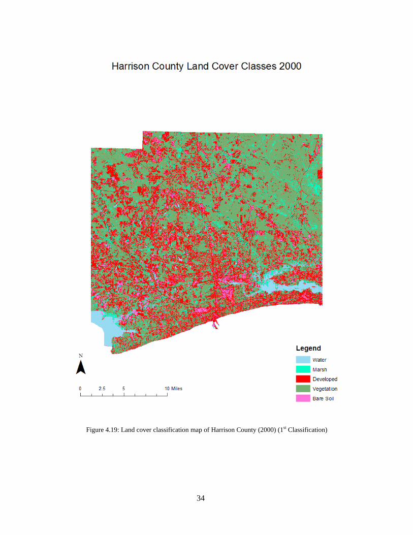
Figure 4.19: Land cover classification map of Harrison County (2000) (1st Classification) .. 34
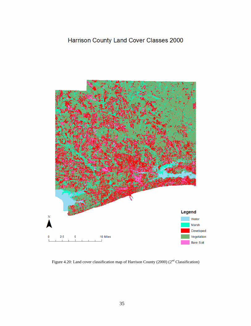
Figure 4.20: Land cover classification map of Harrison County (2000) (2nd Classification) . 35
Figure 4.21: Land cover classification map of Harrison County (2005) ................................ 36
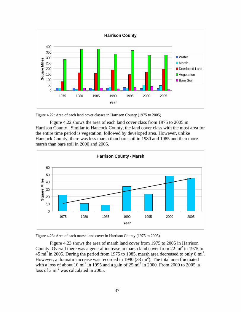
Figure 4.22: Area of each land cover classes in Harrison County (1975 to 2005) ................. 37
Figure 4.23: Area of each marsh land cover in Harrison County (1975 to 2005) .................. 37
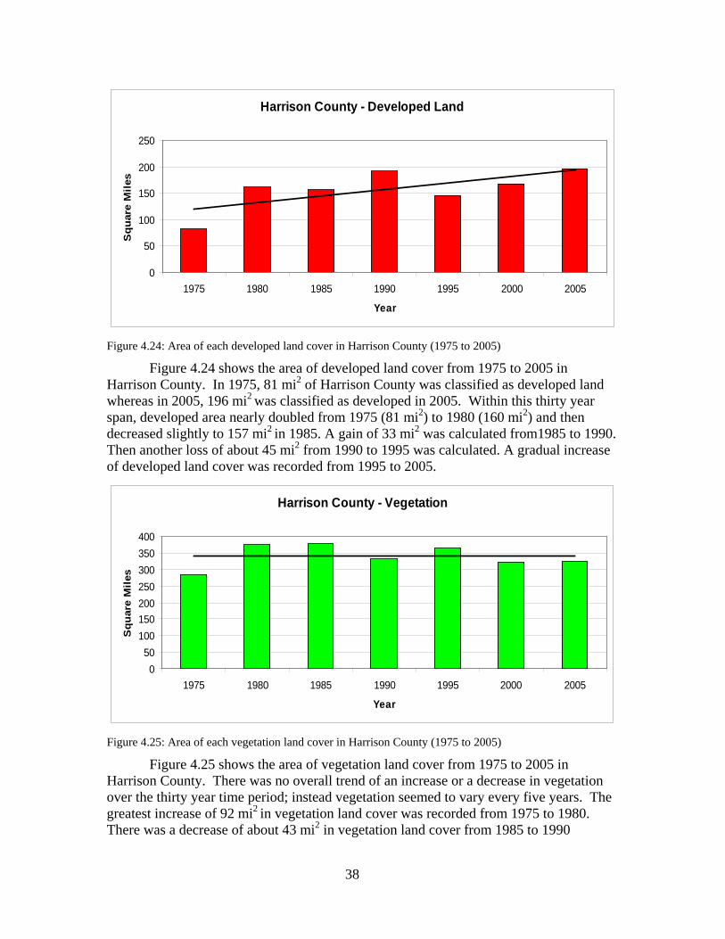
Figure 4.24: Area of each developed land cover in Harrison County (1975 to 2005) ............ 38
v
Figure 4.25: Area of each vegetation land cover in Harrison County (1975 to 2005) ........... 38
Figure 4.26: Area of each bare soil land cover in Harrison County (1975 to 2005) .............. 39
Figure 4.27: Land cover classification map of Jackson County (1975) ................................. 41
Figure 4.28: Land cover classification map of Jackson County (1980) ................................. 42
Figure 4.29: Land cover classification map of Jackson County (1986) ................................. 43
Figure 4.30: Land cover classification map of Jackson County (1990) ................................. 44
Figure 4.31: Land cover classification map of Jackson County (1995) ................................. 45
Figure 4.32: Land cover classification map of Jackson County (2000) (1st Classification) ... 46
Figure 4.33: Land cover classification map of Jackson County (2000) (2nd Classification) .. 47
Figure 4.34: Land cover classification map of Jackson County (2005) ................................. 48
Figure 4.35: Area of each land cover classes in Jackson County (1975 to 2005) .................. 49
Figure 4.36: Area of marsh land cover in Jackson County (1975 to 2005) ............................ 49
Figure 4.37: Area of developed land cover in Jackson County (1975 to 2005) ..................... 50
Figure 4.38: Area of vegetation land cover in Jackson County (1975 to 2005) ..................... 50
Figure 4.39: Area of bare soil land cover in Jackson County (1975 to 2005) ........................ 51
Figure 4.40: Land cover classification map of the Gulf Coast Counties (1975) .................... 52
Figure 4.41: Land cover classification map of the Gulf Coast Counties (1980) .................... 53
Figure 4.42: Land cover classification map of the Gulf Coast Counties (1985-1986) ........... 54
Figure 4.43: Land cover classification map of the Gulf Coast Counties (1990) .................... 55
Figure 4.44: Land cover classification map of the Gulf Coast Counties (1995) .................... 56
Figure 4.45: Land cover classification map of the Gulf Coast Counties (2000) (1st Classification) ................................................................................................................... 57
Figure 4.46: Land cover classification map of the Gulf Coast Counties (2000) (2nd Classification) ................................................................................................................... 58
Figure 4.47: Land cover classification map of the Gulf Coast Counties (2005) .................... 59
Figure 4.48: Area of each land cover classes of the Gulf Coast Counties (1975 to 2005) ..... 60
Figure 4.49: Area of marsh land cover in the Gulf Coast Counties (1975 to 2005) ............... 60
Figure 4.50: Area of developed land cover in the Gulf Coast Counties (1975 to 2005) ........ 61
vi
Figure 4.51: Area of vegetation land cover in the Gulf Coast Counties (1975 to 2005) ........ 61
Figure 4.52: Area of bare soil land cover in the Gulf Coast Counties (1975 to 2005) ........... 62
Figure 5.1: Gulf coast counties population from 1970 to 2005 .............................................. 64
Figure 5.2: Gulf coast counties employment from 1980 to 2000 ........................................... 64
Figure 5.3: Gulf coast counties housing units from 1980 to 2005 .......................................... 65
Figure 5.4: Difference in the amount of each land cover type of two classified 2000 images covering Hancock County ................................................................................................. 66
Figure 5.5: Difference in the amount of each land cover type of two classified 2000 images covering Harrison County ................................................................................................. 67
Figure 5.6: Difference in the amount of each land cover type of two classified 2000 images covering Jackson County .................................................................................................. 67
vii
List of Tables Table 1.1: Anderson’s Level I definitions and examples of land use and land cover types ..... 1
Table 3.1: Satellite image search criteria and results .............................................................. 11
Table 3.2: Descriptions and examples of land use and land cover types ................................ 13
Table 3.3: Population and land cover class correlation. ......................................................... 14
Table 5.1: Gulf Coast County Socioeconomic Factors and Area of each LULC Class Correlation Coefficients .................................................................................................... 65
Table A-1: Gulf Coast Counties raw socioeconomic data ...................................................... 73
viii
List of Acronyms BV Brightness Values C-CAP Coastal Change Analysis Program ERDAS Earth Resource Data Analysis System ESRI Environmental Systems Research Institute ETM Enhanced Thematic Mapper ISODATA Iterative Self Organizing Data Analysis Technique LULC Land Use Land Cover MRLC Multi-resolution land characteristics MSS Multispectral Scanner NDVI Normalized Difference Vegetation Index NLCD National Land Cover Dataset NOAA National Oceanic and Atmospheric Administration NWI National Wetland Inventory SAR Synthetic Aperture Sonar SPOT Satellite Pour l’Observation de la Terre Tif Tagged Imagery File TM Thematic Mapper USGS United States Geological Survey WGS World Geodetic System
ix
Abstract The population, employment and housing units along the Gulf Coast of Mississippi have been increasing since the 1970s through the 2000s. In this study, an overall increasing trend in land cover was found in developed land area near interstates and highways along all three coastal counties. A strong positive correlation was observed in Hancock County between developed land and population and developed land and housing units. A strong negative correlation was observed between vegetation and housing units. Weak positive correlations were found in Harrison County between developed land and population, marsh and population, and marsh and housing units. A weak positive correlation was found in Jackson County between bare soil and population. Several study limitations such as unsupervised classification and misclassification are discussed to explain why a strong correlation was not found in Harrison and Jackson Counties. Land Cover Land Use, Land Cover Classification, Remote Sensing
1
1. Introduction 1.1 Overview of Land Cover / Land Use Research
Land use land cover (LULC) data is “an essential element for modeling and understanding the earth as a system” (Lillesand et al, 2008). Urban planners and government officials use this data for allocation of government resources and policies as well as planning and development purposes. High resolution satellite imagery is readily available and is collected continuously for visual interpretation as well as computer-assisted land cover classification. The term “land use” describes how land is being used by human activity, such as manufacturing or residential areas. Whereas the term “land cover” describes the feature covering the land, such as forest, wetlands, and impervious surfaces (Lillesand et al, 2008).
In the 1970s, United States Geological Survey (USGS) created a LULC classification system for remotely sensed data. Anderson stated that “the classification system has been developed to meet the needs of Federal and State agencies for an up-to-date overview of land use and land cover throughout the country on a basis that is uniform in categorization at the more generalized first and second levels and that will be receptive to data from satellite and aircraft remote sensors” (Anderson et al, 1976). In Anderson’s classification system, there are four levels of LULC classifications; each level is derived from higher resolution remotely sensed imagery. For the purposes of this study, the first level of classification will only be discussed because it pertains to Landsat Thematic Mapper (TM) and Multispectral Scanner (MSS) data resolutions (imagery used in this study). Anderson’s Level I classification types are used for nationwide, interstate and statewide issues because of the spatial resolution of 30 m, an analyst can not distinguish between smaller features measuring less than 30 m. Level I consist of nine types: urban or built-up land, agricultural land, rangeland, forest land, water, wetland, barren land, tundra and perennial snow or ice. Table 1.1 describes the definitions of each LULC type that pertains to Mississippi. Table 1.1: Anderson’s Level I definitions and examples of land use and land cover types Source: Lillesand et al, 2008
LULC Classification Type Definition/Examples
Urban or built-up land Cities, towns, transportation
Agricultural land Land used for natural resource production
Rangeland Land were natural vegetation is grass and where natural grazing is important.
Forest Land Land with tree crown density of 10 percent or more.
Water Streams, canals, lakes, reservoirs, bays and estuaries.
Wetlands Area includes marshes, mudflats, and swamps as well as shallow areas of bays and lakes.
Barren Land with a limited ability to support life.
2
USGS has recently made all archived Landsat imagery from 1975 to the present available to scientific community in the US free of cost. The imagery used in this study was downloaded from USGS Earth Explorer website, further details on data collection can be found in the methodology section. To make this research topic manageable, a time interval was chosen to be five years from 1975 to 2005. The satellite imagery available for this time period was acquired by Landsat MSS and Landsat TM.
Three Landsat satellites were launched in the 1970s; the first Landsat satellite (Landsat-1) was launched in 1972 followed by Landsat-2 in 1975, and in 1978 Landsat-3. Each of these satellites carried a MSS that collected data in four wavelengths regions or spectral bands, Bands 4, 5, 6, and 7. Landsat-1, -2 and -3 had a temporal resolution of 18 days and spatial resolution of 79 m. The spectral resolution of Bands 4, 5, 6 and 7 are 0.5 – 0.6 µm, 0.6 – 0.7 µm, 0.7 – 0.8 µm, and 0.8 – 1.1 µm respectively.
The first Landsat TM satellite was Landsat-4, launched in 1982; however the TM data transmission failed in 1993. Landsat-5 TM, which was launched in March 1984 and collected the imagery from 1985 to 2005, was used in this study. Landsat-5 TM continues to acquire new imagery. Landsat-5 TM has a temporal resolution of 16 days and 30 m spatial resolution in Bands 1, 2, 3, 4, 5 and 7. The bands used in this study are Bands 2, 3, 4 and 5 which are associated with wavelengths considered appropriate for mapping urban features and vegetation types. The wavelengths associated with each Landsat TM band are: 0.52 – 0.60 µm for Band 2 (green), 0.63 – 0.69 µm for Band 3 (red), 0.76 – 0.90 µm for Band 4 (near-infrared) and 1.55 – 1.75 µm for Band 5 (mid-infrared) (Lillesand et al, 2008).
1.2 Land Cover Change Research In 1993, several federal agencies created the Multi-Resolution Land
Characteristics (MRLC) Consortium. The MRLC purchased Landsat-5 imagery that covered the continental United States in order to create a National Land Cover Dataset (NLCD). This first NLCD was published in 1992 and the second NLCD was published in 2001 (Lillesand et al, 2008). These two land cover datasets were used to create the 1992-2001 Land Cover Change Retrofit Product by the USGS which combines the two NLCD datasets to find the change from 1992 and 2001.
1.3 Research Objectives The purpose of this study was to analyze temporal change in land cover through
unsupervised classification of satellite imagery from 1975 to 2005 along the Gulf Coast Counties of Mississippi. Correlation analysis was conducted on several socioeconomic characteristics to determine if there was a possible relationship with the land cover change.
1.4 Organization of the Thesis The thesis is organized into six chapters, beginning with a literature review of
several articles concerning LULC change. Following the literature review, the second chapter gives an overview of the Gulf Coast of Mississippi socioeconomic data from the 1970 through 2005. The third chapter describes the methodology for this study by detailing the data collection of the satellite imagery and socioeconomic data, data organization, and finally data analysis. This is followed by the results and discussion of
3
the research objective and issues with the study. Lastly, the conclusion summarizes the important findings of this study and what these findings could mean for Gulf Coast residents. References are listed at the end of the thesis. The raw socioeconomic data is found in tabular format in Appendix A.
4
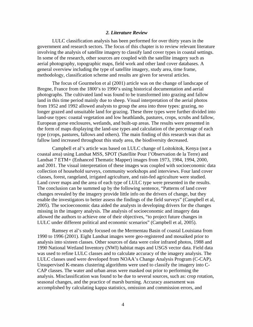
2. Literature Review LULC classification analysis has been performed for over thirty years in the
government and research sectors. The focus of this chapter is to review relevant literature involving the analysis of satellite imagery to classify land cover types in coastal settings. In some of the research, other sources are coupled with the satellite imagery such as aerial photography, topographic maps, field work and other land cover databases. A general overview including the type of satellite imagery, study area, time frame, methodology, classification scheme and results are given for several articles.
The focus of Gourmelon et al (2001) article was on the change of landscape of Bregne, France from the 1800’s to 1990’s using historical documentation and aerial photographs. The cultivated land was found to be transformed into grazing and fallow land in this time period mainly due to sheep. Visual interpretation of the aerial photos from 1952 and 1992 allowed analysts to group the area into three types: grazing, no longer grazed and unsuitable land for grazing. These three types were further divided into land-use types: coastal vegetation and low heathlands, pastures, crops, scrubs and fallow, European gorse enclosures, wetlands, and built-up areas. The results were presented in the form of maps displaying the land-use types and calculation of the percentage of each type (crops, pastures, fallows and others). The main finding of this research was that as fallow land increased throughout this study area, the biodiversity decreased.
Campbell et al’s article was based on LULC change of Loitokitok, Kenya (not a coastal area) using Landsat MSS, SPOT (Satellite Pour l’Observation de la Terre) and Landsat 7 ETM+ (Enhanced Thematic Mapper) images from 1973, 1984, 1994, 2000, and 2001. The visual interpretation of these images was coupled with socioeconomic data collection of household surveys, community workshops and interviews. Four land cover classes, forest, rangeland, irrigated agriculture, and rain-fed agriculture were studied. Land cover maps and the area of each type of LULC type were presented in the results. The conclusion can be summed up by the following sentence, “Patterns of land cover changes revealed by the imagery provide little info on the drivers of change, but they enable the investigators to better assess the findings of the field surveys” (Campbell et al, 2005). The socioeconomic data aided the analysts in developing drivers for the changes missing in the imagery analysis. The analysis of socioeconomic and imagery data allowed the authors to achieve one of their objectives, “to project future changes in LULC under different political and economic scenarios” (Campbell et al, 2005).
Ramsey et al’s study focused on the Mermentau Basin of coastal Louisiana from 1990 to 1996 (2001). Eight Landsat images were geo-registered and mosaiked prior to analysis into sixteen classes. Other sources of data were color infrared photos, 1988 and 1990 National Wetland Inventory (NWI) habitat maps and USGS vector data. Field data was used to refine LULC classes and to calculate accuracy of the imagery analysis. The LULC classes used were developed from NOAA’s Change Analysis Program (C-CAP). Unsupervised K-means clustering algorithms were used to classify the imagery into C-CAP classes. The water and urban areas were masked out prior to performing the analysis. Misclassification was found to be due to several sources, such as: crop rotation, seasonal changes, and the practice of marsh burning. Accuracy assessment was accomplished by calculating kappa statistics, omission and commission errors, and
5
verification by other NOAA personnel not involved in classification as well as field analysis.
Ramsey et al also conducted change detection analysis, which involved post classification analysis using all sixteen classes. A matrix of from-to land cover class was constructed. Two indications of class stability, location and residence were developed. Location stability was calculated from the percent of LULC class that stayed the same during the study period while the residence stability was calculated from the percentage change in each class within the study area. The results were presented as the area of each LULC class and the change between three time periods, 1990 to 1993, 1993 to 1996 and 1990 to 1996. LULC maps and the percentage of each type of the entire study were also presented. The change analysis revealed that about half of the LULC classes experienced little or no change. Five principal findings from this research are listed below:
1. “Land cover turnover is maintaining a near stable logging cycle, but grassland, scrub shrub and forest in cycle appeared to change.
2. Planting of seedlings is critical to maintaining cycle stability.
3. Logging activities tend to replace woody land mixed forests with woody land evergreen forests.
4. Wetland estuarine marshes are expanding slightly.
5. Wetland palustrine marshes and mature forested wetlands are relatively stable (Ramsey et al, 2001).”
The goal of the Kandus et al (1999) study was to create a LULC classification scheme “to understand the interaction between the natural and man-made ecosystems that coexist in the [Argentina] delta islands.” Aerial photos and field data collected from 1984 to 1990 was analyzed along with three Landsat TM images from 1993. The Landsat imagery was corrected for geometric and radiometric distortion corrections using topographic maps in ERDAS (Earth Resource Data Analysis System). Unsupervised ISODATA (Iterative Self Organizing Data Analysis Technique) classification was conducted on the three images. The user’s, producer’s, and overall accuracy was calculated as the result of this study. The classification scheme was found to be flexible conceptually which allowed for aggregation and desegregation of land cover classes as required and not defined by satellite imagery.
The Klemas et al (1993) article focused on the development of a land cover classification scheme for the C-CAP covering coastal wetlands, uplands, and submerged habitats mainly for fisheries habitat and marine resources management. The scheme was adapted from several sources (Anderson et al, 1976; Cowardin et al, 1979; and USGS, 1992). C-CAP is a program to monitor areas of significant change and serves as a database for coastal land cover based on satellite imagery (Landsat MSS, TM, and SPOT). This classification scheme is compatible with NOAA’s National Marine Fisheries Service and the NWI. Products of research with the C-CAP classification scheme are spatially registered digital images, hard copy maps, and summary tables. Five attributes of the C-CAP classification scheme are listed below:
1. “Emphasizes wetlands, vegetated submersed habitats, and adjacent uplands,”
6
2. Upland classes developed from Anderson et al (1976), USGS (1992) and modifications Cowardin et al (1979).
3. Classes defined primarily in terms of land cover vice land use
4. Hierarchical classification scheme
5. Scheme designed to use satellite (TM and SPOT) data and also be compatible with aerial and field data (Klemas et al, 1993).
Huang et al’s 2008 study focused on Synthetic Aperture Radar (SAR) images from 2002 of coastal China. Radar was used because of the cloudy weather often found along the China coast. Six main steps were discussed in the methods section, such as 1) SAR noise despeckle, 2) dike extraction, 3) spatial zoning, 4) backscattering coefficient conversion, 5) textual analysis and 6) image classification. Two techniques were used for image classification, unsupervised ISODATA and supervised back-propagation neural network (an iterative gradient algorithm). The classification scheme used in this study was based on Anderson et al (1976) Level 1, 2, and 3. The results were presented in a percentage of each land cover type in five delineated zones. The SAR imagery was “able to produce almost identical and acceptable levels of class accuracy” (Huang et al, 2008).
Qi et al’s study focused on Laizhou Gulf Coast of China, an area with fast economic development (2008). Landsat TM imagery from 1988 to 2002 was analyzed in IDRISI software to georeference the imagery to topographic maps and classify into six LULC classes modified from the USGS LULC classification system (2008). The six classes used for this study were cropland, forestland, grassland, urban and/or built-up land, water and barren land. Accuracy of the imagery classification was calculated from stratified random sampling methods to generate reference points for each classification images. Also, general LC delineations on topographic maps, municipal maps, and field surveys were also used to verify the imagery LULC classification technique. Field investigations also involved social, economic, and anthropogenic data. The conclusion of the study was summarized by the following statement, “the land-use pattern in saltwater intrusion areas was altered and the landscapes of coastal plains were modified in a considerably short period, owing to the impacts of both natural conditions and human activities, especially the saltwater intrusion induced by the latter” (Qi et al, 2008).
Hanamgond and Mitra’s study focused on the morphological features of Mahashta, India using Landsat TM an ETM Images from 1989 and 1999. Five land classes were analyzed in the imagery, such as agriculture, forest, beach and alluvial sand, marshy/mangrove, and grassland/plantation. The methodology included supervised classification and image differencing. The change in area and percentage of each class was presented in the results of this study. Two generations of beach ridges were found to correspond with periods of accretion and erosion.
Everitt et al (2008) used Quickbird imagery for “mapping [of] black mangrove along the south Texas Gulf Coast.” Each image used in this study was classified using supervised and unsupervised image analysis techniques. Five training sites coupled with a max likelihood classifier were chosen for the supervised classification technique. The max likelihood classifier method classified two images of the study sites using the signatures from each of the five classes extracted from the training sites. The five LULC
7
classes used for this study were black mangrove, wet soil, seagrass, mixed vegetation, soil or roads and water. ISODATA was used for the unsupervised classification technique. Ground truthing was used to calculate overall accuracy; producer’s and user’s accuracy as well as the kappa coefficient were also calculated. The accuracy of using these methods to classify the imagery was found to range from very good to excellent.
Carreno et al (2007) used multitemporal Landsat TM and ETM imagery acquired from 1984 to 2000 to study vegetal communities and hydrological dynamics in wetlands of the Mar Menor Lagoon in Spain. In 1979, the Tagus-Segura water transfer system opened and since then an increase in nutrient inputs has been recorded coming from the irrigated lands into the lagoon and surrounding wetlands. Temporal change was calculated by analyzing the land cover change in the initial imagery (1984) to final imagery (2001). Regression analysis between the wetland area and irrigated lands was also presented in the results of this study. A confusion matrix was created to characterize error and accuracy coefficients. In conclusion, an overall increase in total wetland area found to be a poor indicator of the increase in water input at the watershed scale because “the increase in hygrophilous vegetation observed overall…. [which] constitutes a good indicator of such water changes;” however, a significant relationship was found between the irrigated lands surrounding the lagoon and wetlands and the area of the salt marsh and reed beds in the wetlands (Carreno et al, 2007).
Brown et al (2005) focused on “dominant spatial and temporal trends in population, agriculture and urbanized land uses” through the United States from 1950 to 2000. A second focus of this article was to present the results of LULC change from remote sensing data from 1973 to 2000. The article did not go into detail describing the methodology for the remote sensing data; however the authors did mention that the USGS land cover data was manually interpreted from the imagery. The distribution of population served an indicator for demand for various goods and services provided by ecological systems. A pocket of loss in the MS Delta was interpreted in the data. Also the population all across the country moved to more metropolitan areas from the 1950s to 2000s. Urbanization defined as the “expansion of urban land uses, including commercial, industrial and residential” (Brown et al, 2005). A few agricultural trends worth noting are that overall area of cropland decreased by 11% from 1950 to 2000 (35% to 31% of the land); the Mississippi Delta was one of the exceptions of this trend. In summary, “remote sensing methodologies provide a means for better quantifying changes along the urban to rural gradient, but collection of land use data through on-the-ground surveys are also needed” (Brown et al, 2005).
Hilbert (2006) conducted LULC classification of the Grand Bay National Estuarine Research Reserve of Mississippi, an undisturbed estuarine marsh-pine savannah habitats surrounding the Gulf of Mexico. Three Landsat images from 1974, 1991 and 2001 were analyzed by unsupervised classification and change detection techniques. The LC classes used for this study were open water, herbaceous wetland, forest and barren land. NDVI (Normalized Difference Vegetation Index) was calculated and then the unsupervised classification method was run on the data. It relied on ISODATA to create the four clusters of LC. The change detection technique involved change matrices derived from post-classification pairs of successive image dates. There was no field work related to this study, the LC results were compared to the NLCD 1992
8
dataset. The change detection analysis amplified what was already known about the anthropogenic stressors that affect the biodiversity of the area; i.e. substantial land development, dredging and spoil placement in Pascagoula has led to estuarine habitat loss. The LULC maps developed from the study indicated “that the majority of land cover change between 1974 and 2001 occurred as a results of expansion of open water and a reduction in wetland” (Hilbert 2006).
Collins et al (2005) focused on Mississippi forest cover changes and regeneration dates. Five LULC classes were specifically developed for this study. The methodology involved ISODATA clustering as part of the first stage of post-classification followed by step-wise reduction of classification. The step-wise classification was used to determine the regeneration/origin date of the forest cover pixel by pixel. Temporal differences in vegetation were determined by analysis of NDVI and Tasseled Cap images. A Simultaneous Image Difference process was run on the imagery which involved: masking of pixels, stacking of masks, max likelihood processing applied to the signatures and data overlay to create a final forest age thematic map of the six different age classes. An accuracy assessment was also conducted that uncovered poor accuracy levels possibly due to the errors during the georectification process and the Tasseled Cap transformation (Collins et al, 2005).
Oivanki et al (1995) focused on Mississippi Gulf Coast Wetlands along four drainage basins and their total loss and gain from the 1950s to 1990s. Seven classes were used in this study developed by Cowardin et al in 1979. The methodology for this study involved airphoto interpretation and manual digitization of the 1990 data as well as the transfer of historical data from the 1950s and 1970s from tape to a machine. The historical imagery was also digitized into the LULC classes. The results included maps that depicted the total land area gained, total land area lost and total marsh (wetland) lost from 1950s to 1990s (Oivanki et al, 1995).
O’Hara et al (2003) focused on the Mississippi Coastal Counties and their urban areas from 1970s to 2000. Six LULC Anderson Level 1 and 2 classes were used in this study. The methodology to classify the land cover and find the changes involved unsupervised classification, supervised classification and thematic change and formal rule-based classification. The results of this analysis were two figures displaying the “Thematic Representation of Classified Areas in 1991” and the “Amount of Change in Each Area 1991 to 2000” (O’Hara et al, 2003). An accuracy assessment was also conducted on the LULC results presented in the study, values of 90% and 85% were found for the Level 1 and 2 classifications respectively (O’Hara et al, 2003).
9
3. Methods 3.1 Data Collection
3.1.1 Socioeconomic Data The socioeconomic data used in this study included county level census
population, employment, and housing unit data from 1970 to 2005. This data was compiled from several online resources, such as the Mississippi Center for Population Studies and U.S. Census Bureau. The raw data is found in Table A-1 in Appendix A. Estimates in population, employment and housing units were used for the intercensal years. It is important to note that housing unit data were not available for 1970, 1975, 1985, and 1995. Also, employment data was not available for 1970, 1975, and 1985. The main purpose of the socioeconomic data was to relate the results of the land cover analysis to possible reasons for land cover change; therefore an incomplete socioeconomic dataset is satisfactory for the purpose of this study.
The population data is defined as the number of people within each county for the census year (1980, 1990, and 2000). Employment is defined as the number of workers who were employed within the county for the census year. Housing units are defined by the U.S. Census as “a house, an apartment, a mobile home, a group of rooms, or a single room that is occupied (or if vacant, is intended for occupancy) as separate living quarters” for the census year (State Data Center, 2001). The 1985, 1995 and 2005 population estimates are averages as of July 1 of the corresponding year. The 2005 housing unit estimates were based on estimates as of July 1, 2005. The 1995 employment estimates were the average labor force by county (no specific date). The 2005 employment estimates were from Quarter 1 “total number of workers who were employed by the same employer in both the current and previous quarter” (U.S. Census Bureau, 2009).
Several spreadsheets in Microsoft Excel were created to organize the data and to determine which counties to focus on for this study. Differences between each decadal dataset were compiled, for example the 1990 population was subtracted from the 2000 population to calculate change between the two decades. Next, the dataset was sorted for each timeframe (2000 to 1990) from highest to lowest amount of change in population and county employment. Ten counties with the most and least amount of change in 2000 were then ranked for each of the other timeframes, 1990-1980 and 1980-1970, to see how each county changed over the study period. The coastal counties of Hancock, Harrison, and Jackson, were found to be in the top ten counties in the state of Mississippi with the most population growth. These counties were also found to have growth in county employment as well. From this analysis, these counties were selected for land cover analysis in this study.
3.1.2 Satellite Imagery The satellite imagery used for this study was Landsat 4-5 TM and Landsat 1-5
MSS. This imagery was available for free of cost at the USGS website, Earth Explorer, http://edcsns17.cr.usgs.gov/EarthExplorer. Landsat Imagery is organized in paths and rows, and in order to determine the correct paths and rows that covered the study area, one image from each of the paths 20 through 23 and rows 38 through 39 were acquired.
10
These paths and rows were determined from analysis of the Landsat Path/Row Map shown in Figure 3.1. One band from each of these images was then displayed in ESRI (Environmental Systems Research Institute) ArcMap software along with the MafTiger Census 2000 County Boundaries shapefiles of Hancock, Harrison, and Jackson. The path/rows of Landsat TM that covered the Coast Counties of Mississippi were found to be paths 21 through 22 and row 39. The path/rows of Landsat MSS were found to be path 22 through 23 and row 39.
Figure 3.1: WRS-2 path /row (Landsats 4, 5, and 7) and UTM zones Source: http://landsat.gsfc.nasa.gov/about/wrs2.gif
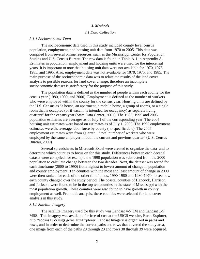
The next step was to define search criteria from the USGS Earth Explorer website in order to find the satellite imagery that covered the study area within the study’s time frame, 1975 through 2005, in five year intervals. Images with less than 10 percent cloud cover were also added to the search criteria; however this information was not always recorded in the metadata therefore images with clouds were inadvertently downloaded. A summary of the image search criteria and the number of images returned are found in Table 3.1. All images were either available for immediate download or had to be ordered. If an image had to be ordered, it would usually take a few days to be staged for download. A total of 111 images were found to fit these search criteria. These files were then downloaded into path / row folders on to an external hard drive for extra storage.
11
Table 3.1: Satellite image search criteria and results
3.2 Imagery Data Organization
The satellite imagery was downloaded from the website in zipped tar file format with the file extension .tar.gz. These files were saved into the appropriate path/row folders. Next, the tar files were uncompressed by a dos script that put them in file folders with the same name as the tar.gz file. The Landsat TM tar files were uncompressed into seven tifs (one for each band 1 through 7) and the appropriate metadata files. The Landsat MSS were compressed into four tifs (one for each band 4 through 7) and the appropriate metadata files. Tifs (Tagged Imagery File) is a file format for storing imagery files.
3.3 Imagery Data Analysis 3.3.1 Imagery Preprocessing The multi-temporal comparison of LULC change required image analysis
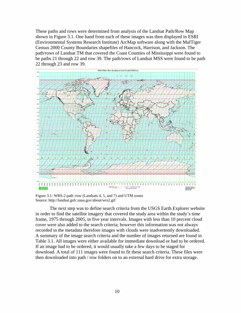
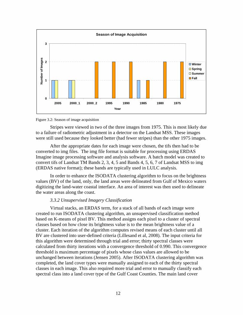
acquisition dates near the same time of year. In order to identify the images with acquisition dates within the same month, a spreadsheet was created to visualize all of the images collected and their acquisition dates effectively. The path/row combinations of the images were listed as column headers while the Julian dates were listed on the rows within the spreadsheet. Checks were used to mark the collection dates for each image. The potential images for analysis in this study were then imported into ERDAS to check the image quality. Each image was then examined for the amount and extent of cloud coverage. Imagery with serious clouds coverage or other quality issues was excluded from further analysis. Images acquired in the summer months were found to have clouds; therefore most of the images used in this thesis were acquired in the fall and winter months. Figure 3.2 shows the number images used in each year’s analysis and the season the image was acquired. A total of sixteen images were analyzed for this study, two per year for eight time periods.
12
Season of Image Acquisition
0
1
2
3
2005 2000_1 2000_2 1995 1990 1985 1980 1975
Year
Num
ber o
f Im
ages
WinterSpringSummerFall
Figure 3.2: Season of image acquisition
Stripes were viewed in two of the three images from 1975. This is most likely due to a failure of radiometric adjustment in a detector on the Landsat MSS. These images were still used because they looked better (had fewer stripes) than the other 1975 images.
After the appropriate dates for each image were chosen, the tifs then had to be converted to img files. The img file format is suitable for processing using ERDAS Imagine image processing software and analysis software. A batch model was created to convert tifs of Landsat TM Bands 2, 3, 4, 5 and Bands 4, 5, 6, 7 of Landsat MSS to img (ERDAS native format); these bands are typically used in LULC analysis.
In order to enhance the ISODATA clustering algorithm to focus on the brightness values (BV) of the land, only, the land areas were delineated from Gulf of Mexico waters digitizing the land-water coastal interface. An area of interest was then used to delineate the water areas along the coast.
3.3.2 Unsupervised Imagery Classification Virtual stacks, an ERDAS term, for a stack of all bands of each image were
created to run ISODATA clustering algorithm, an unsupervised classification method based on K-means of pixel BV. This method assigns each pixel to a cluster of spectral classes based on how close its brightness value is to the mean brightness value of a cluster. Each iteration of the algorithm computes revised means of each cluster until all BV are clustered into user-defined criteria (Lillesand et al, 2008). The input criteria for this algorithm were determined through trial and error; thirty spectral classes were calculated from thirty iterations with a convergence threshold of 0.990. This convergence threshold is maximum percentage of pixels whose class values are allowed to be unchanged between iterations (Jensen 2005). After ISODATA clustering algorithm was completed, the land cover types were manually assigned to each of the thirty spectral classes in each image. This also required more trial and error to manually classify each spectral class into a land cover type of the Gulf Coast Counties. The main land cover
13
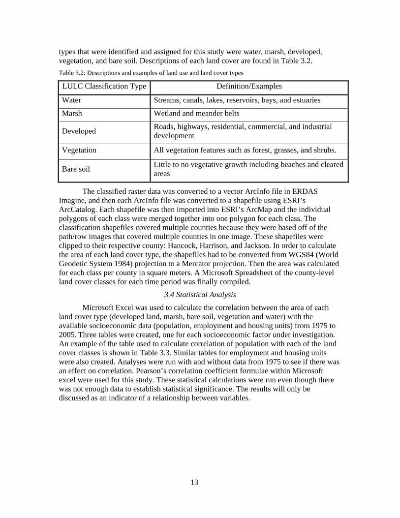
types that were identified and assigned for this study were water, marsh, developed, vegetation, and bare soil. Descriptions of each land cover are found in Table 3.2. Table 3.2: Descriptions and examples of land use and land cover types
LULC Classification Type Definition/Examples
Water Streams, canals, lakes, reservoirs, bays, and estuaries
Marsh Wetland and meander belts
Developed Roads, highways, residential, commercial, and industrial development
Vegetation All vegetation features such as forest, grasses, and shrubs.
Bare soil Little to no vegetative growth including beaches and cleared areas
The classified raster data was converted to a vector ArcInfo file in ERDAS Imagine, and then each ArcInfo file was converted to a shapefile using ESRI’s ArcCatalog. Each shapefile was then imported into ESRI’s ArcMap and the individual polygons of each class were merged together into one polygon for each class. The classification shapefiles covered multiple counties because they were based off of the path/row images that covered multiple counties in one image. These shapefiles were clipped to their respective county: Hancock, Harrison, and Jackson. In order to calculate the area of each land cover type, the shapefiles had to be converted from WGS84 (World Geodetic System 1984) projection to a Mercator projection. Then the area was calculated for each class per county in square meters. A Microsoft Spreadsheet of the county-level land cover classes for each time period was finally compiled.
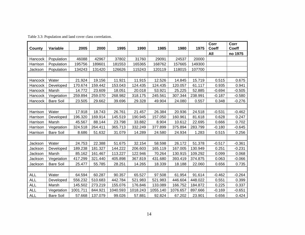
3.4 Statistical Analysis Microsoft Excel was used to calculate the correlation between the area of each
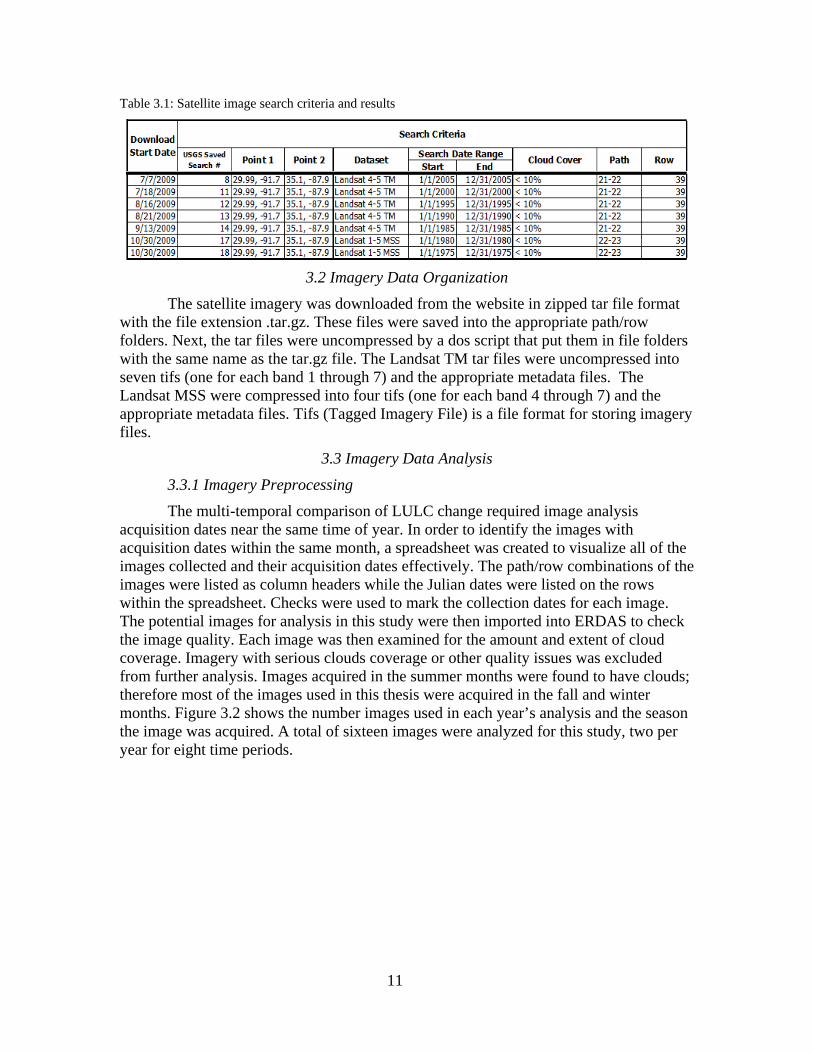
land cover type (developed land, marsh, bare soil, vegetation and water) with the available socioeconomic data (population, employment and housing units) from 1975 to 2005. Three tables were created, one for each socioeconomic factor under investigation. An example of the table used to calculate correlation of population with each of the land cover classes is shown in Table 3.3. Similar tables for employment and housing units were also created. Analyses were run with and without data from 1975 to see if there was an effect on correlation. Pearson’s correlation coefficient formulae within Microsoft excel were used for this study. These statistical calculations were run even though there was not enough data to establish statistical significance. The results will only be discussed as an indicator of a relationship between variables.
14
Table 3.3: Population and land cover class correlation.
County Variable 2005 2000 1995 1990 1985 1980 1975 Corr Coeff
Corr Coeff
All no 1975 Hancock Population 46088 42967 37802 31760 29091 24537 20000 Harrison Population 195756 189601 181553 165365 168762 157665 149300 Jackson Population 134243 131420 126626 115243 120119 118015 107700 Hancock Water 21.924 19.156 11.921 11.915 12.526 14.845 15.719 0.515 0.675 Hancock Developed 170.674 159.442 153.043 124.435 124.435 120.057 61.117 0.935 0.941 Hancock Marsh 14.772 23.609 18.051 20.018 53.921 25.225 52.885 -0.694 -0.505 Hancock Vegetation 259.894 259.070 268.982 318.175 245.561 307.344 238.991 -0.187 -0.580 Hancock Bare Soil 23.505 29.662 39.696 29.328 49.904 24.080 0.557 0.348 -0.276 Harrison Water 17.918 18.743 26.761 21.457 26.384 20.936 24.518 -0.531 -0.462 Harrison Developed 196.320 169.914 145.519 190.945 157.050 160.961 81.618 0.628 0.247 Harrison Marsh 45.567 88.144 23.798 33.882 8.904 10.612 22.695 0.666 0.702 Harrison Vegetation 324.518 264.411 365.713 332.249 377.899 375.894 283.799 -0.180 -0.645 Harrison Bare Soil 8.686 51.632 31.079 14.289 24.580 24.934 1.283 0.515 0.256 Jackson Water 24.753 22.388 51.675 32.154 58.598 26.172 51.378 -0.517 -0.361 Jackson Developed 189.238 181.327 144.222 206.603 165.119 167.005 130.949 0.251 -0.231 Jackson Marsh 85.162 161.467 113.227 122.946 70.264 130.915 109.292 0.099 0.068 Jackson Vegetation 417.299 321.440 405.898 367.819 431.680 393.419 374.875 0.063 -0.066 Jackson Bare Soil 25.477 55.785 28.251 14.265 18.339 18.188 22.060 0.656 0.735 ALL Water 64.594 60.287 90.357 65.527 97.508 61.954 91.614 -0.462 -0.264 ALL Developed 556.232 510.683 442.784 521.983 521.983 446.604 448.022 0.551 0.399 ALL Marsh 145.502 273.219 155.076 176.846 133.089 166.752 184.872 0.225 0.337 ALL Vegetation 1001.711 844.921 1040.593 1018.243 1055.140 1076.657 897.666 -0.169 -0.651 ALL Bare Soil 57.668 137.079 99.026 57.881 92.824 67.202 23.901 0.656 0.424
15
4. Results The purpose of this study was to analyze temporal change in land cover through
unsupervised classification of satellite imagery from 1975 to 2005 along the Gulf Coast Counties of Mississippi. The results chapter is organized into three sections, one for each Mississippi Gulf Coast County, Hancock, Harrison and Jackson County. Within each section, land cover classification maps for each year 1975 through 2005 are presented after a description of the changes are detailed. The thematic maps are large therefore they follow the description of the changes observed starting in 1975. Following the thematic maps, charts showing the area of each land cover class (developed area, marsh, vegetation, and bare soil) are described in detail. A description of the water class was not included because the focus of this study was mostly on land cover types.
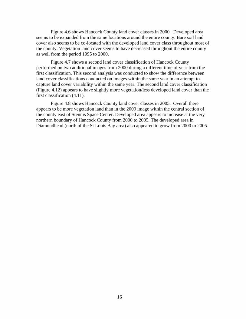
4.1 Hancock County Land Cover Analysis Figure 4.1 shows Hancock County land cover classes in 1975. The marsh area is
present along the southwest coast of the county and in the St Louis Bay area. Developed land appears to be located in Bay St Louis, and the area north of I-10 in the form of small patches. The State Road 607 and Highway 90 are also visible as developed area south of I-10. The bad data values are shown in grey and appear as diagonal lines through the other land cover classes.
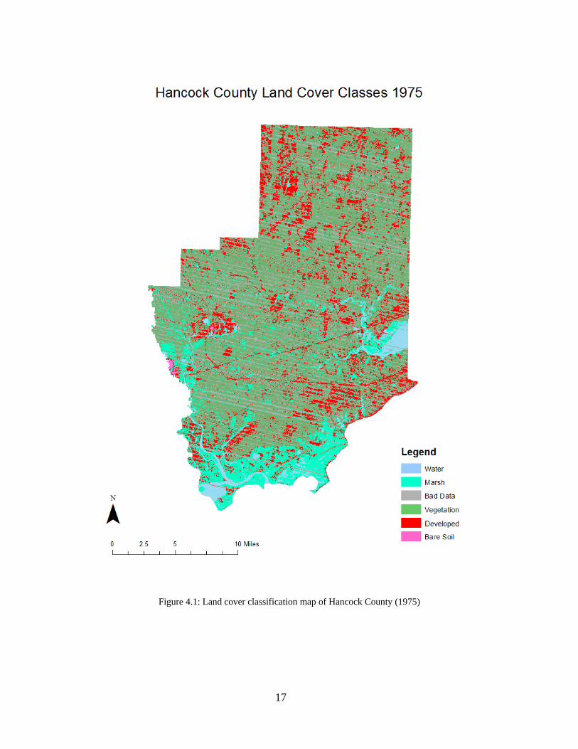
Figure 4.2 shows Hancock County land cover classes in 1980. In 1980, the marsh area appears to be less around the Pearl River watershed than in 1975. Land previously classified as vegetation in 1975 was classified as developed in the 1980 map. Developed land cover appears to cover more area than the 1975 image especially in Bay St Louis, Waveland and northern part of the county, east of Highway 53. Stennis Space Center also appears to be more developed in 1980 than in 1975. Bare soil appears to around boundaries of the developed areas in the northern section of the county as well as within the marshes of Waveland and with the entrance to Diamondhead.
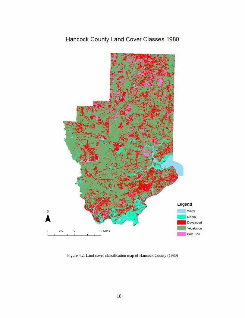
The 1985 land cover classification map of Hancock County is shown in Figure 4.3. Developed land cover in the northern section of Hancock County appears to have increased from 1980 to 1985. Some of the land cover south of I-10 in Waveland and in Diamondhead classified as developed land in 1980 was classified as bare soil in the 1985 map. This change in classification could mean that the developed land was converted to bare soil from 1980 to 1985.
Figure 4.4 shows Hancock County land cover classes in 1990. Developed areas in the northern section of the county appear to have been converted to the vegetation cover class from 1985 to 1990. Also, there does not appear to be as much bare soil classified around developed cover area in Bay St Louis and Waveland area. Vegetation land cover class appears to have increased along the central section of the county during the period from 1985 to 1990.
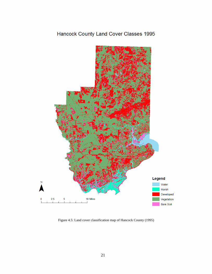
Figure 4.5 shows Hancock County land cover classes in 1995. When comparing the 1995 land cover classification map to the 1985 and 1990 maps, the developed area appears to have increased along the central section of the county near Highway 603 and Highway 53. Waveland also appears to have more developed land cover than vegetation land cover from 1990 to 1995.
16
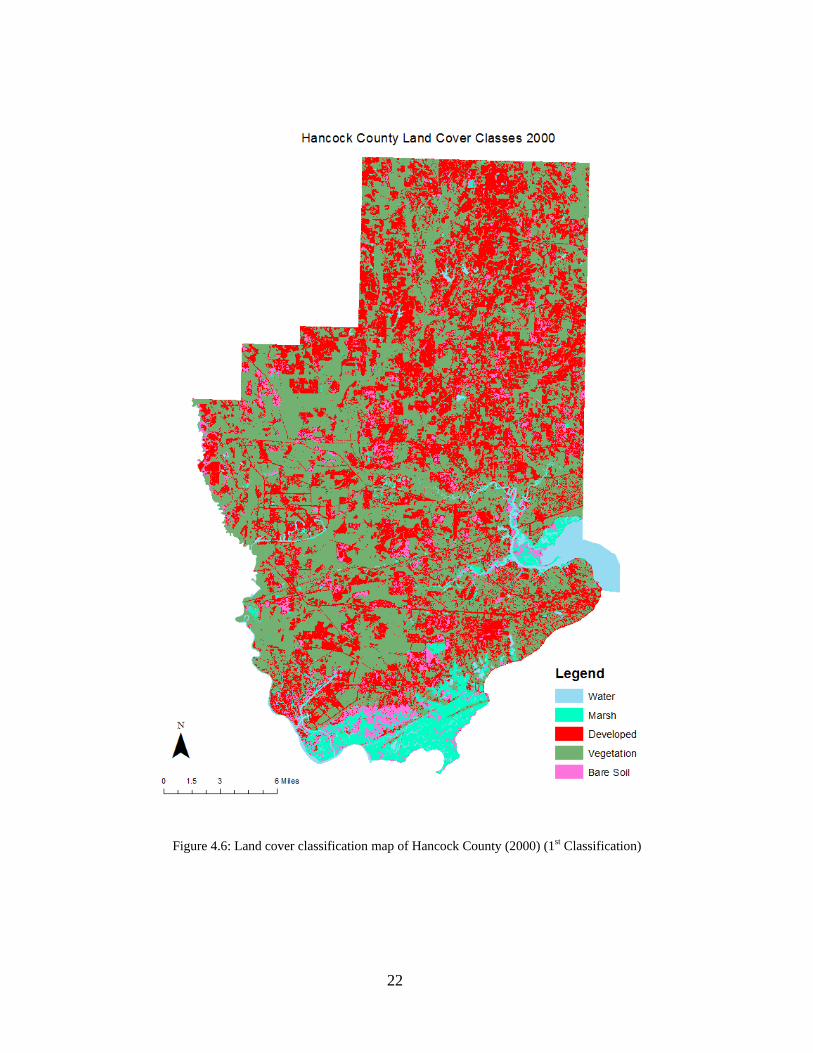
Figure 4.6 shows Hancock County land cover classes in 2000. Developed area seems to be expanded from the same locations around the entire county. Bare soil land cover also seems to be co-located with the developed land cover class throughout most of the county. Vegetation land cover seems to have decreased throughout the entire county as well from the period 1995 to 2000.
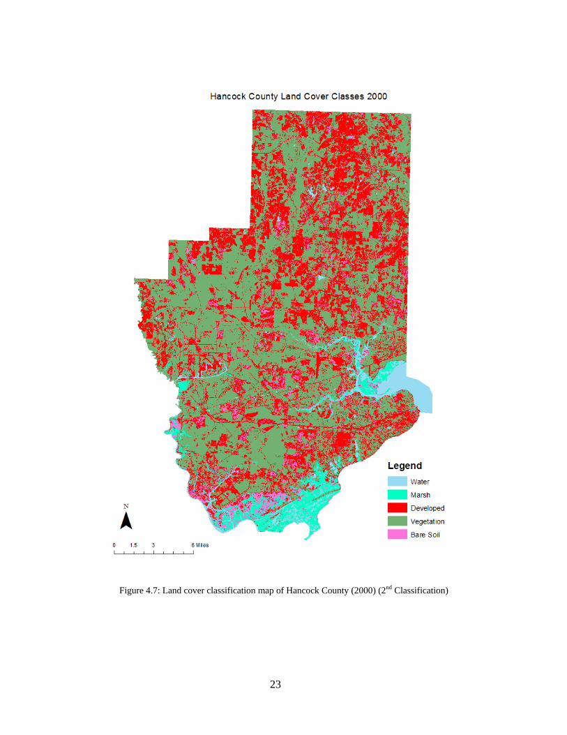
Figure 4.7 shows a second land cover classification of Hancock County performed on two additional images from 2000 during a different time of year from the first classification. This second analysis was conducted to show the difference between land cover classifications conducted on images within the same year in an attempt to capture land cover variability within the same year. The second land cover classification (Figure 4.12) appears to have slightly more vegetation/less developed land cover than the first classification (4.11).
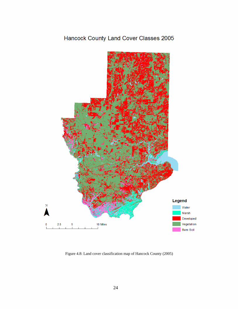
Figure 4.8 shows Hancock County land cover classes in 2005. Overall there appears to be more vegetation land than in the 2000 image within the central section of the county east of Stennis Space Center. Developed area appears to increase at the very northern boundary of Hancock County from 2000 to 2005. The developed area in Diamondhead (north of the St Louis Bay area) also appeared to grow from 2000 to 2005.
17
Figure 4.1: Land cover classification map of Hancock County (1975)
18
Figure 4.2: Land cover classification map of Hancock County (1980)
19
Figure 4.3: Land cover classification map of Hancock County (1985)

20
Figure 4.4: Land cover classification map of Hancock County (1990)
21
Figure 4.5: Land cover classification map of Hancock County (1995)
22
Figure 4.6: Land cover classification map of Hancock County (2000) (1st Classification)
23
Figure 4.7: Land cover classification map of Hancock County (2000) (2nd Classification)
24
Figure 4.8: Land cover classification map of Hancock County (2005)
25
Hancock County
0
50
100
150
200
250
300
350
1975 1980 1985 1990 1995 2000 2005
Year
Squ
are
Mile
s Water MarshDeveloped LandVegetationBare Soil
Figure 4.9: Area of each land cover classes in Hancock County (1975 to 2005)
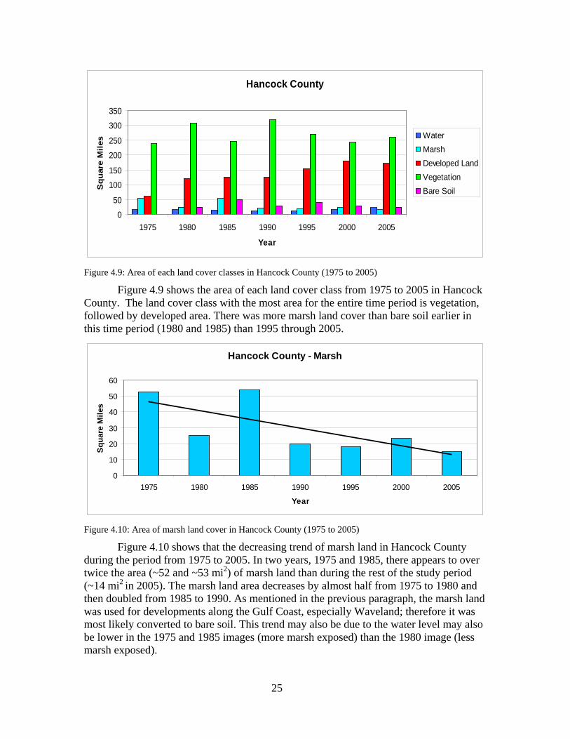
Figure 4.9 shows the area of each land cover class from 1975 to 2005 in Hancock County. The land cover class with the most area for the entire time period is vegetation, followed by developed area. There was more marsh land cover than bare soil earlier in this time period (1980 and 1985) than 1995 through 2005.
Hancock County - Marsh
0
10
20
30
40
50
60
1975 1980 1985 1990 1995 2000 2005
Year
Squa
re M
iles
Figure 4.10: Area of marsh land cover in Hancock County (1975 to 2005)
Figure 4.10 shows that the decreasing trend of marsh land in Hancock County during the period from 1975 to 2005. In two years, 1975 and 1985, there appears to over twice the area (~52 and ~53 mi2) of marsh land than during the rest of the study period (~14 mi2 in 2005). The marsh land area decreases by almost half from 1975 to 1980 and then doubled from 1985 to 1990. As mentioned in the previous paragraph, the marsh land was used for developments along the Gulf Coast, especially Waveland; therefore it was most likely converted to bare soil. This trend may also be due to the water level may also be lower in the 1975 and 1985 images (more marsh exposed) than the 1980 image (less marsh exposed).
26
Hancock County - Developed Land
0
50
100
150
200
1975 1980 1985 1990 1995 2000 2005
Year
Squ
are
Mile
s
Figure 4.11: Area of developed land cover in Hancock County (1975 to 2005)
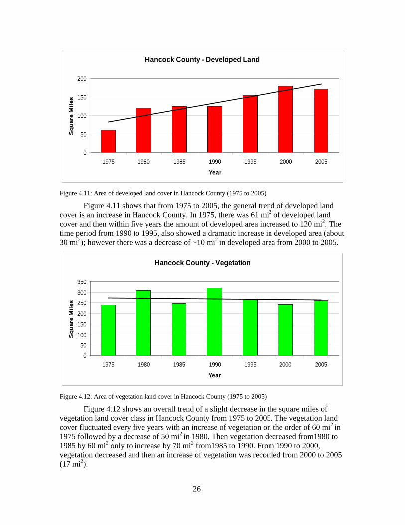
Figure 4.11 shows that from 1975 to 2005, the general trend of developed land cover is an increase in Hancock County. In 1975, there was 61 mi2 of developed land cover and then within five years the amount of developed area increased to 120 mi2. The time period from 1990 to 1995, also showed a dramatic increase in developed area (about 30 mi2); however there was a decrease of ~10 mi2 in developed area from 2000 to 2005.
Hancock County - Vegetation
0
50
100
150
200
250
300
350
1975 1980 1985 1990 1995 2000 2005
Year
Squ
are
Mile
s
Figure 4.12: Area of vegetation land cover in Hancock County (1975 to 2005)
Figure 4.12 shows an overall trend of a slight decrease in the square miles of vegetation land cover class in Hancock County from 1975 to 2005. The vegetation land cover fluctuated every five years with an increase of vegetation on the order of 60 mi2 in 1975 followed by a decrease of 50 mi2 in 1980. Then vegetation decreased from1980 to 1985 by 60 mi2 only to increase by 70 mi2 from1985 to 1990. From 1990 to 2000, vegetation decreased and then an increase of vegetation was recorded from 2000 to 2005 (17 mi2).
27
Hancock County - Bare Soil
0
10
20
30
40
50
60
1975 1980 1985 1990 1995 2000 2005
Year
Squ
are
Mile
s
Figure 4.13: Area of bare soil cover in Hancock County (1975 to 2005)
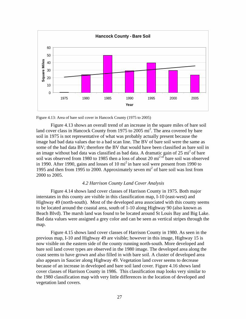
Figure 4.13 shows an overall trend of an increase in the square miles of bare soil land cover class in Hancock County from 1975 to 2005 mi2. The area covered by bare soil in 1975 is not representative of what was probably actually present because the image had bad data values due to a bad scan line. The BV of bare soil were the same as some of the bad data BV; therefore the BV that would have been classified as bare soil in an image without bad data was classified as bad data. A dramatic gain of 25 mi2 of bare soil was observed from 1980 to 1985 then a loss of about 20 mi2 of bare soil was observed in 1990. After 1990, gains and losses of 10 mi2 in bare soil were present from 1990 to 1995 and then from 1995 to 2000. Approximately seven mi2 of bare soil was lost from 2000 to 2005.
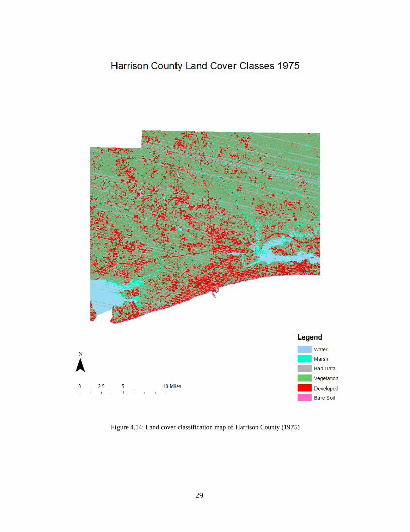
4.2 Harrison County Land Cover Analysis Figure 4.14 shows land cover classes of Harrison County in 1975. Both major
interstates in this county are visible in this classification map, I-10 (east-west) and Highway 49 (north-south). Most of the developed area associated with this county seems to be located around the coastal area, south of 1-10 along Highway 90 (also known as Beach Blvd). The marsh land was found to be located around St Louis Bay and Big Lake. Bad data values were assigned a grey color and can be seen as vertical stripes through the map.
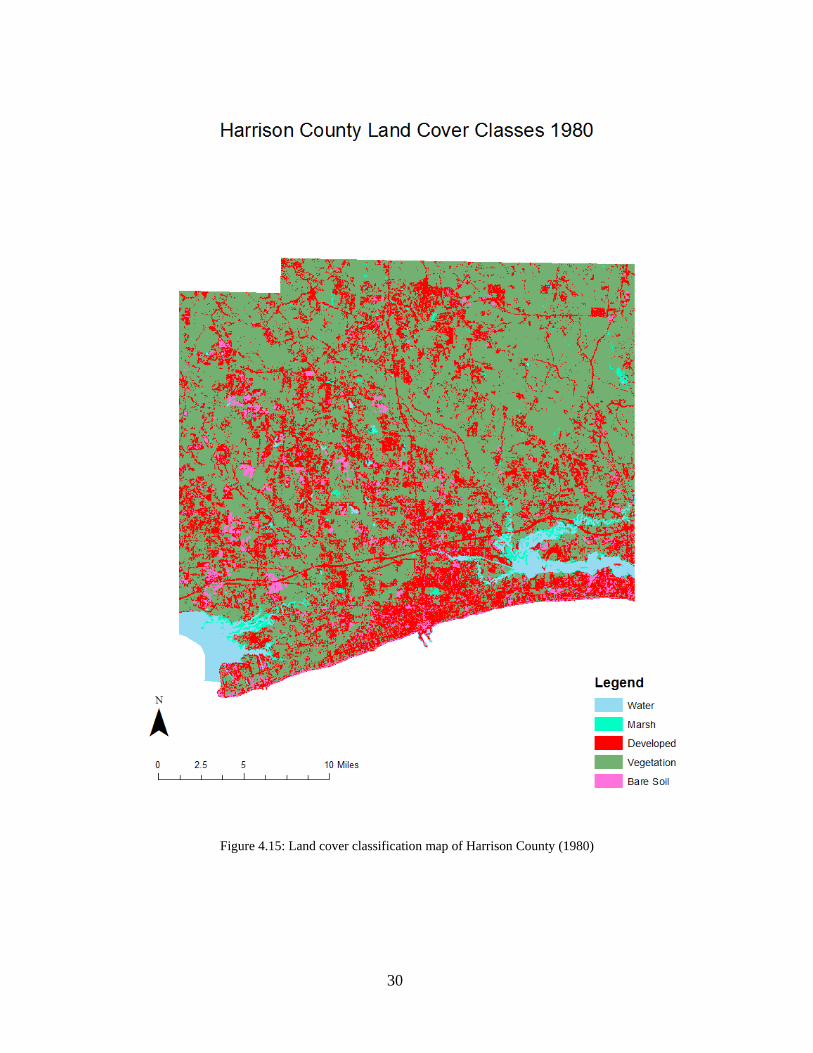
Figure 4.15 shows land cover classes of Harrison County in 1980. As seen in the previous map, I-10 and Highway 49 are visible; however in this image, Highway 15 is now visible on the eastern side of the county running north-south. More developed and bare soil land cover types are observed in the 1980 image. The developed area along the coast seems to have grown and also filled in with bare soil. A cluster of developed area also appears in Saucier along Highway 49. Vegetation land cover seems to decrease because of an increase in developed and bare soil land cover. Figure 4.16 shows land cover classes of Harrison County in 1986. This classification map looks very similar to the 1980 classification map with very little differences in the location of developed and vegetation land covers.
28
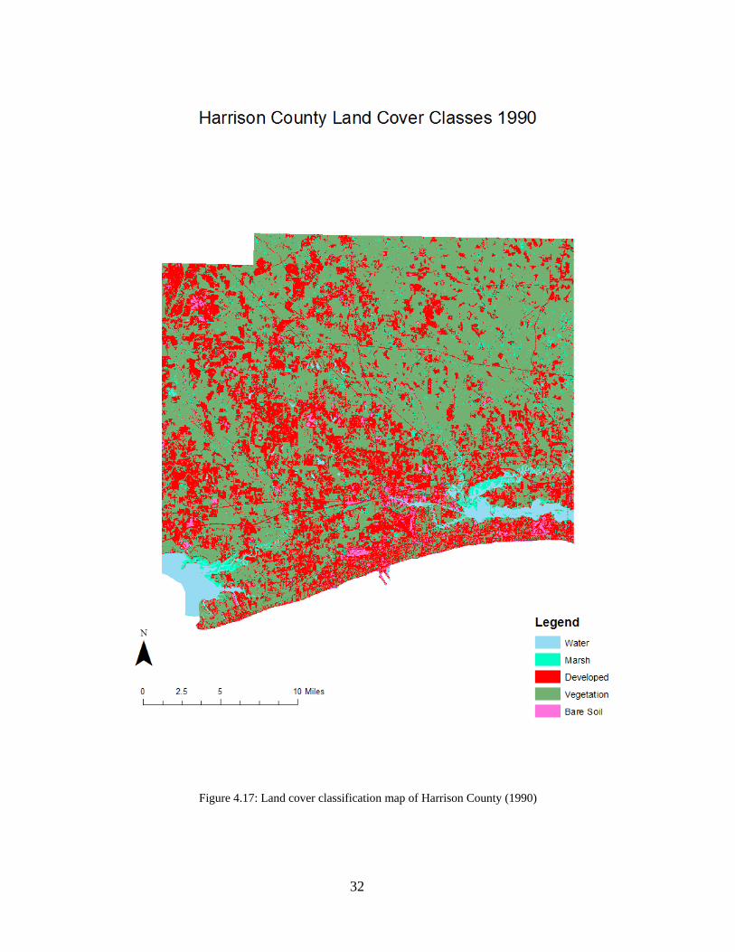
Figure 4.17 shows land cover classes of Harrison County in 1990. The developed land cover along the coast remains about the same while most of the change appears in the northern section of the county. Developed area around Saucier appears to have been converted to vegetation while area in the northwest corner appears to be more developed. This area is most likely used for agriculture versus traditional developed area with homes and business buildings. The developed land cover doesn’t appear to have straight lines that are a feature of man-made structures.
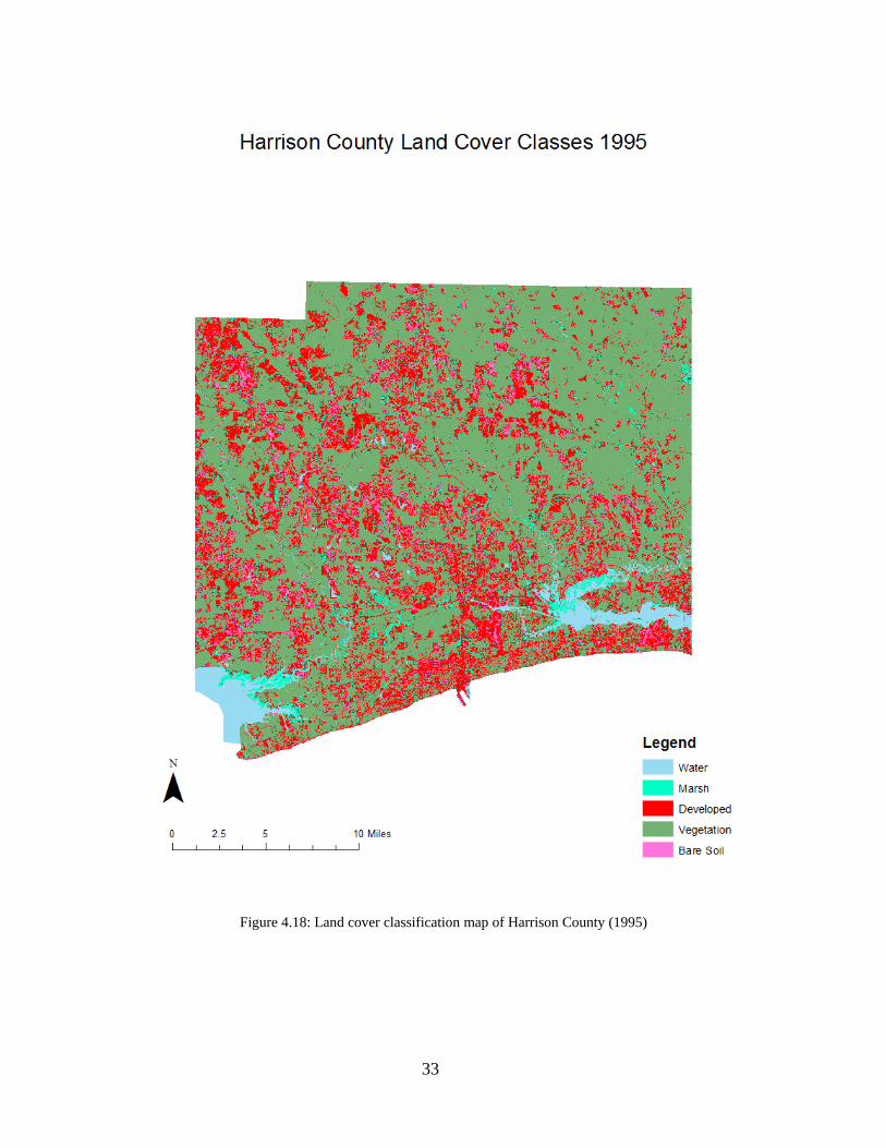
Figure 4.18 shows land cover classes of Harrison County in 1995. Developed and bare soil land cover area seems to have decreased from 1990. More vegetation land cover is present where land was previously classified as developed land. Highway 15 seems to have disappeared and changed to vegetation in some areas of the northern portion of the route.
Figure 4.19 shows land cover classes of Harrison County in 2000. More developed and bare soil land cover appears in this image than the 1995 image. Most of the developed area appears in the lower half of the county, along the coast and north to the middle of the map. Bare soil land cover was found to be attached to developed land cover area with a large cluster around the Gulfport Airport and Naval Seabee Base. Also, marsh land cover appears to be located throughout the county’s small water bodies in the northeast section of the county; however the majority of the northeast section of the county still appears to be composed of mostly vegetation.
Figure 4.20 shows the second land cover classification maps shows of Harrison County conducted on second set of imagery from 2000. This second analysis was conducted to show the difference between land cover classifications conducted on images within the same year in an attempt to capture land cover variability within the same year. The second land cover classification (Figure 4.20) appears to have slightly more bare soil land cover that was classified as developed land cover in the first classification (Figure 4.19).
Figure 4.21 shows land cover classes of Harrison County in 2005. The amount of developed area in this map appears to be unchanged from 2000. The marsh area seems to have increased in areas formerly classified as vegetation located in the northwest section of the county in the 2000 map. Areas classified as bare soil in the first classification of 2000 imagery appears to be classified as developed land cover in the 2005 map, such as the Gulfport Airport and Naval Seabee Base.
29
Figure 4.14: Land cover classification map of Harrison County (1975)
30
Figure 4.15: Land cover classification map of Harrison County (1980)

31
Figure 4.16: Land cover classification map of Harrison County (1986)
32
Figure 4.17: Land cover classification map of Harrison County (1990)
33
Figure 4.18: Land cover classification map of Harrison County (1995)
34
Figure 4.19: Land cover classification map of Harrison County (2000) (1st Classification)
35
Figure 4.20: Land cover classification map of Harrison County (2000) (2nd Classification)

36
Figure 4.21: Land cover classification map of Harrison County (2005)
37
Harrison County
050
100150200250300350400
1975 1980 1985 1990 1995 2000 2005
Year
Squ
are
Mile
s Water MarshDeveloped LandVegetationBare Soil
Figure 4.22: Area of each land cover classes in Harrison County (1975 to 2005)
Figure 4.22 shows the area of each land cover class from 1975 to 2005 in Harrison County. Similar to Hancock County, the land cover class with the most area for the entire time period is vegetation, followed by developed area. However, unlike Hancock County, there was less marsh than bare soil in 1980 and 1985 and then more marsh than bare soil in 2000 and 2005.
Harrison County - Marsh
0
10
20
30
40
50
60
1975 1980 1985 1990 1995 2000 2005
Year
Squ
are
Mile
s
Figure 4.23: Area of each marsh land cover in Harrison County (1975 to 2005)
Figure 4.23 shows the area of marsh land cover from 1975 to 2005 in Harrison County. Overall there was a general increase in marsh land cover from 22 mi2 in 1975 to 45 mi2 in 2005. During the period from 1975 to 1985, marsh area decreased to only 8 mi2. However, a dramatic increase was recorded in 1990 (33 mi2). The total area fluctuated with a loss of about 10 mi2 in 1995 and a gain of 25 mi2 in 2000. From 2000 to 2005, a loss of 3 mi2 was calculated in 2005.
38
Harrison County - Developed Land
0
50
100
150
200
250
1975 1980 1985 1990 1995 2000 2005
Year
Squ
are
Mile
s
Figure 4.24: Area of each developed land cover in Harrison County (1975 to 2005)
Figure 4.24 shows the area of developed land cover from 1975 to 2005 in Harrison County. In 1975, 81 mi2 of Harrison County was classified as developed land whereas in 2005, 196 mi2 was classified as developed in 2005. Within this thirty year span, developed area nearly doubled from 1975 (81 mi2) to 1980 (160 mi2) and then decreased slightly to 157 mi2 in 1985. A gain of 33 mi2 was calculated from1985 to 1990. Then another loss of about 45 mi2 from 1990 to 1995 was calculated. A gradual increase of developed land cover was recorded from 1995 to 2005.
Harrison County - Vegetation
050
100150200250300350400
1975 1980 1985 1990 1995 2000 2005
Year
Squ
are
Mile
s
Figure 4.25: Area of each vegetation land cover in Harrison County (1975 to 2005)
Figure 4.25 shows the area of vegetation land cover from 1975 to 2005 in Harrison County. There was no overall trend of an increase or a decrease in vegetation over the thirty year time period; instead vegetation seemed to vary every five years. The greatest increase of 92 mi2 in vegetation land cover was recorded from 1975 to 1980. There was a decrease of about 43 mi2 in vegetation land cover from 1985 to 1990
39
followed by an increase of 33 mi2 in 1995. A decrease of 44 mi2 was recorded from 1995 to 2000. In 2005, a slight increase of about 3 mi2 in vegetation land cover from 2000 to 2005.
Harrison County - Bare Soil
05
10152025303540
1975 1980 1985 1990 1995 2000 2005
Year
Squ
are
Mile
s
Figure 4.26: Area of each bare soil land cover in Harrison County (1975 to 2005)
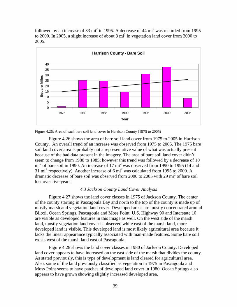
Figure 4.26 shows the area of bare soil land cover from 1975 to 2005 in Harrison County. An overall trend of an increase was observed from 1975 to 2005. The 1975 bare soil land cover area is probably not a representative value of what was actually present because of the bad data present in the imagery. The area of bare soil land cover didn’t seem to change from 1980 to 1985; however this trend was followed by a decrease of 10 mi2 of bare soil in 1990. An increase of 17 mi2 was observed from 1990 to 1995 (14 and 31 mi2 respectively). Another increase of 6 mi2 was calculated from 1995 to 2000. A dramatic decrease of bare soil was observed from 2000 to 2005 with 29 mi2 of bare soil lost over five years.
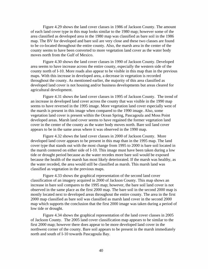
4.3 Jackson County Land Cover Analysis Figure 4.27 shows the land cover classes in 1975 of Jackson County. The center
of the county starting in Pascagoula Bay and north to the top of the county is made up of mostly marsh and vegetation land cover. Developed areas are mostly concentrated around Biloxi, Ocean Springs, Pascagoula and Moss Point. U.S. Highway 90 and Interstate 10 are visible as developed features in this image as well. On the west side of the marsh land, mostly vegetation land cover is observed while east of the marsh land, more developed land is visible. This developed land is most likely agricultural area because it lacks the linear appearance typically associated with man-made features. Some bare soil exists west of the marsh land east of Pascagoula.
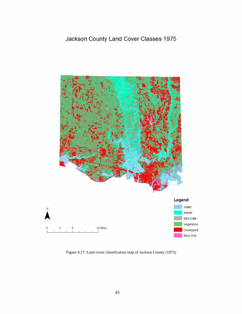
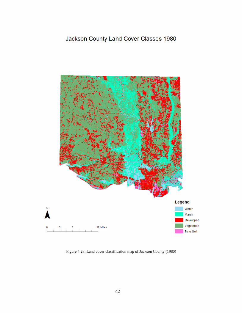
Figure 4.28 shows the land cover classes in 1980 of Jackson County. Developed land cover appears to have increased on the east side of the marsh that divides the county. As stated previously, this is type of development is land cleared for agricultural area. Also, some of the land previously classified as vegetation in 1975 in Pascagoula and Moss Point seems to have patches of developed land cover in 1980. Ocean Springs also appears to have grown showing slightly increased developed area.
40
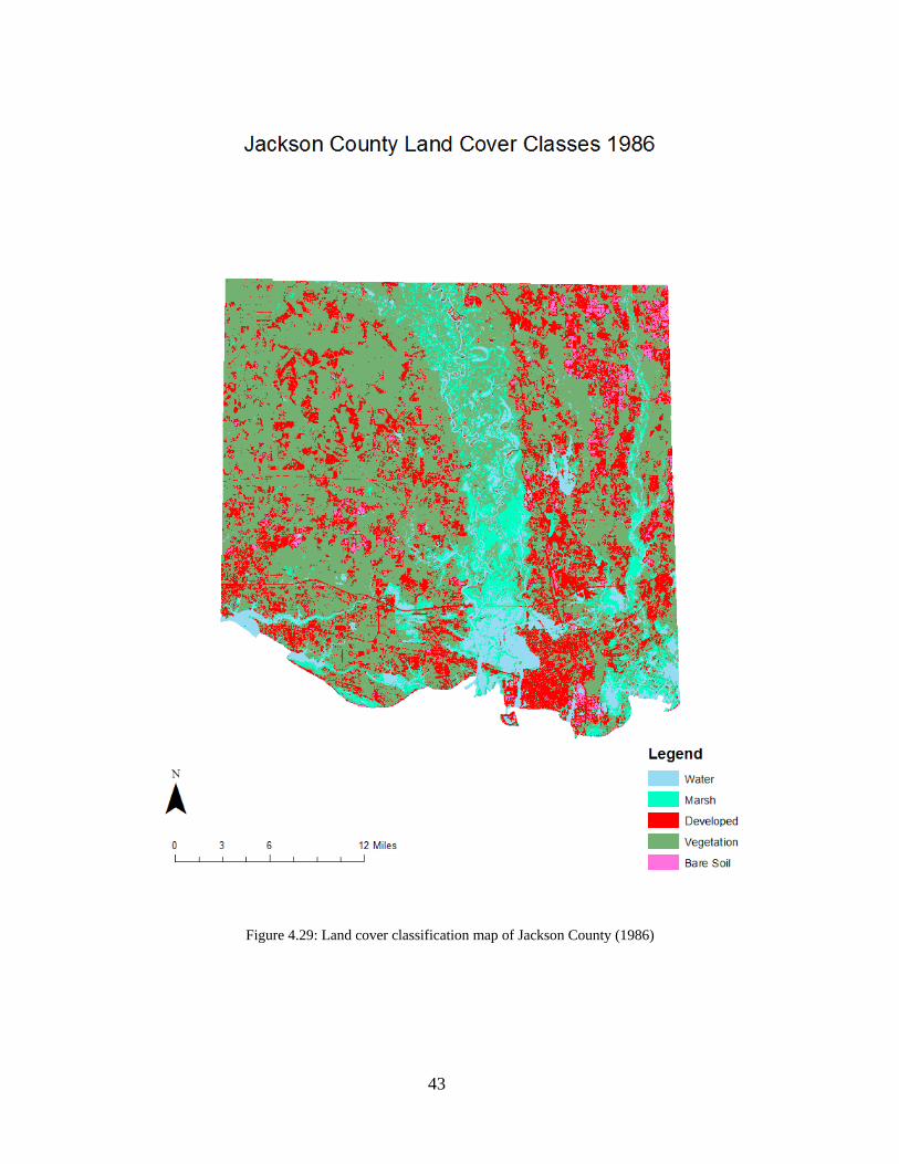
Figure 4.29 shows the land cover classes in 1986 of Jackson County. The amount of each land cover type in this map looks similar to the 1980 map; however some of the area classified as developed area in the 1980 map was classified as bare soil in the 1986 map. The BV for developed and bare soil are very close and these two classes are found to be co-located throughout the entire county. Also, the marsh area in the center of the county seems to have been converted to more vegetation land cover as the water body moves north from the Gulf of Mexico.
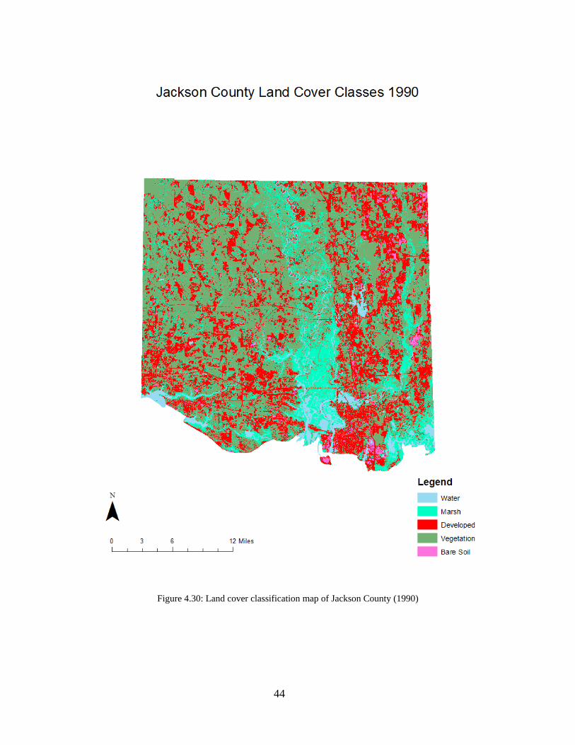
Figure 4.30 shows the land cover classes in 1990 of Jackson County. Developed area seems to have increase across the entire county, especially the western side of the county north of I-10. More roads also appear to be visible in this map than in the previous maps. With this increase in developed area, a decrease in vegetation is recorded throughout the county. As mentioned earlier, the majority of this area classified as developed land cover is not housing and/or business developments but areas cleared for agricultural development.
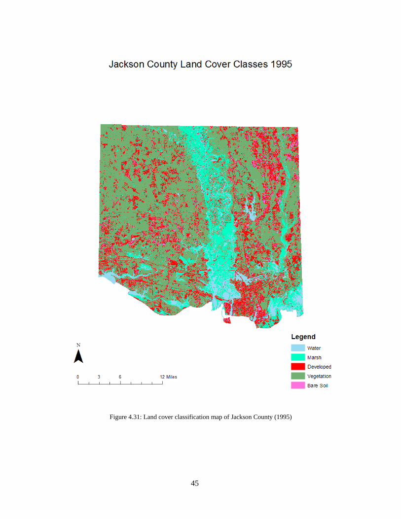
Figure 4.31 shows the land cover classes in 1995 of Jackson County. The trend of an increase in developed land cover across the county that was visible in the 1990 map seems to have reversed in the 1995 image. More vegetation land cover especially west of the marsh is present in this image when compared to the 1990 image. Also, some vegetation land cover is present within the Ocean Spring, Pascagoula and Moss Point developed areas. Marsh land cover seems to have regained the former vegetation land cover in the center of the county as the water body moves north. Bare soil land cover appears to be in the same areas where it was observed in the 1990 map.
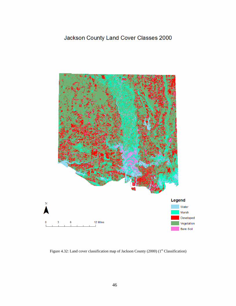
Figure 4.32 shows the land cover classes in 2000 of Jackson County. More developed land cover appears to be present in this map than in the 1995 map. The land cover type that stands out with the most change from 1995 to 2000 is bare soil located in the marsh centered on either side of I-10. This image must have been taken during a low tide or drought period because as the water recedes more bare soil would be exposed because the health of the marsh has most likely deteriorated. If the marsh was healthy, as the water receded, the area would still be classified as marsh. This marsh land was classified as vegetation in the previous maps.
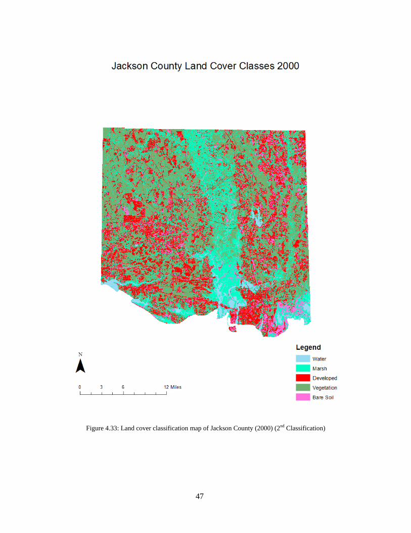
Figure 4.33 shows the graphical representation of the second land cover classification of an imagery acquired in 2000 of Jackson County. This map shows an increase in bare soil compares to the 1995 map; however, the bare soil land cover is not observed in the same place as the first 2000 map. The bare soil in the second 2000 map is mostly located next to developed areas throughout the entire county. The area in the first 2000 map classified as bare soil was classified as marsh land cover in the second 2000 map which supports the conclusion that the first 2000 image was taken during a period of low tide or drought.
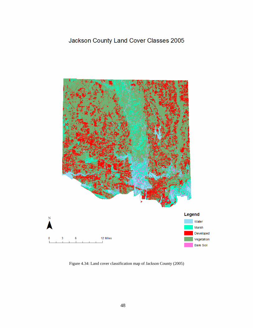
Figure 4.34 shows the graphical representation of the land cover classes in 2005 of Jackson County. The 2005 land cover classification map appears to be similar to the first 2000 map; however there does appear to be more developed land cover in the northwest corner of the county. Bare soil appears to be present in the marsh immediately north and south of I-10 towards Pascagoula Bay.
41
Figure 4.27: Land cover classification map of Jackson County (1975)
42
Figure 4.28: Land cover classification map of Jackson County (1980)
43
Figure 4.29: Land cover classification map of Jackson County (1986)
44
Figure 4.30: Land cover classification map of Jackson County (1990)
45
Figure 4.31: Land cover classification map of Jackson County (1995)
46
Figure 4.32: Land cover classification map of Jackson County (2000) (1st Classification)
47
Figure 4.33: Land cover classification map of Jackson County (2000) (2nd Classification)
48
Figure 4.34: Land cover classification map of Jackson County (2005)
49
Jackson County
0
100
200
300
400
500
1975 1980 1985 1990 1995 2000 2005
Year
Squa
re M
iles Water
MarshDeveloped LandVegetationBare Soil
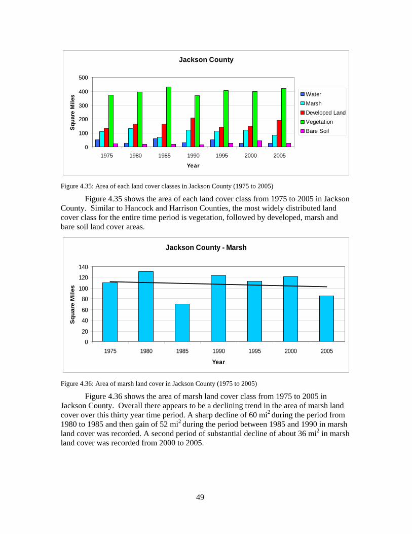
Figure 4.35: Area of each land cover classes in Jackson County (1975 to 2005)
Figure 4.35 shows the area of each land cover class from 1975 to 2005 in Jackson County. Similar to Hancock and Harrison Counties, the most widely distributed land cover class for the entire time period is vegetation, followed by developed, marsh and bare soil land cover areas.
Jackson County - Marsh
0
20
40
60
80
100
120
140
1975 1980 1985 1990 1995 2000 2005
Year
Squ
are
Mile
s
Figure 4.36: Area of marsh land cover in Jackson County (1975 to 2005)
Figure 4.36 shows the area of marsh land cover class from 1975 to 2005 in Jackson County. Overall there appears to be a declining trend in the area of marsh land cover over this thirty year time period. A sharp decline of 60 mi2 during the period from 1980 to 1985 and then gain of 52 mi2 during the period between 1985 and 1990 in marsh land cover was recorded. A second period of substantial decline of about 36 mi2 in marsh land cover was recorded from 2000 to 2005.
50
Jackson County - Developed Land
0
50
100
150
200
250
1975 1980 1985 1990 1995 2000 (1st) 2005
Year
Squ
are
Mile
s
Figure 4.37: Area of developed land cover in Jackson County (1975 to 2005)
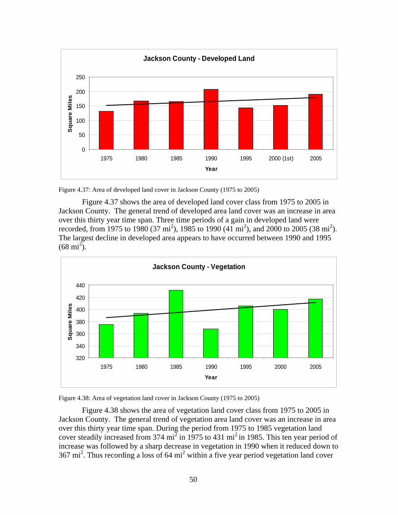
Figure 4.37 shows the area of developed land cover class from 1975 to 2005 in Jackson County. The general trend of developed area land cover was an increase in area over this thirty year time span. Three time periods of a gain in developed land were recorded, from 1975 to 1980 (37 mi2), 1985 to 1990 (41 mi2), and 2000 to 2005 (38 mi2). The largest decline in developed area appears to have occurred between 1990 and 1995 (68 mi2).
Jackson County - Vegetation
320
340
360
380
400
420
440
1975 1980 1985 1990 1995 2000 2005
Year
Squ
are
Mile
s
Figure 4.38: Area of vegetation land cover in Jackson County (1975 to 2005)
Figure 4.38 shows the area of vegetation land cover class from 1975 to 2005 in Jackson County. The general trend of vegetation area land cover was an increase in area over this thirty year time span. During the period from 1975 to 1985 vegetation land cover steadily increased from 374 mi2 in 1975 to 431 mi2 in 1985. This ten year period of increase was followed by a sharp decrease in vegetation in 1990 when it reduced down to 367 mi2. Thus recording a loss of 64 mi2 within a five year period vegetation land cover
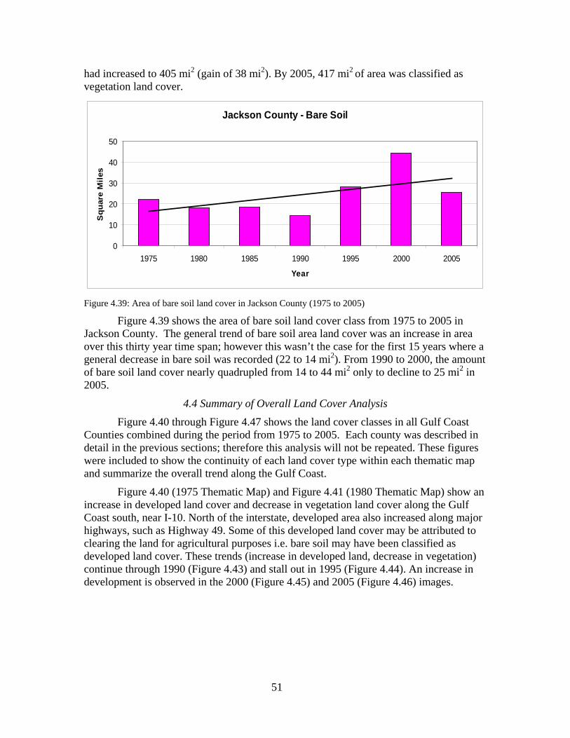
51
had increased to 405 mi2 (gain of 38 mi2). By 2005, 417 mi2 of area was classified as vegetation land cover.
Jackson County - Bare Soil
0
10
20
30
40
50
1975 1980 1985 1990 1995 2000 2005
Year
Squ
are
Mile
s
Figure 4.39: Area of bare soil land cover in Jackson County (1975 to 2005)
Figure 4.39 shows the area of bare soil land cover class from 1975 to 2005 in Jackson County. The general trend of bare soil area land cover was an increase in area over this thirty year time span; however this wasn’t the case for the first 15 years where a general decrease in bare soil was recorded (22 to 14 mi2). From 1990 to 2000, the amount of bare soil land cover nearly quadrupled from 14 to 44 mi2 only to decline to 25 mi2 in 2005.
4.4 Summary of Overall Land Cover Analysis Figure 4.40 through Figure 4.47 shows the land cover classes in all Gulf Coast
Counties combined during the period from 1975 to 2005. Each county was described in detail in the previous sections; therefore this analysis will not be repeated. These figures were included to show the continuity of each land cover type within each thematic map and summarize the overall trend along the Gulf Coast.
Figure 4.40 (1975 Thematic Map) and Figure 4.41 (1980 Thematic Map) show an increase in developed land cover and decrease in vegetation land cover along the Gulf Coast south, near I-10. North of the interstate, developed area also increased along major highways, such as Highway 49. Some of this developed land cover may be attributed to clearing the land for agricultural purposes i.e. bare soil may have been classified as developed land cover. These trends (increase in developed land, decrease in vegetation) continue through 1990 (Figure 4.43) and stall out in 1995 (Figure 4.44). An increase in development is observed in the 2000 (Figure 4.45) and 2005 (Figure 4.46) images.
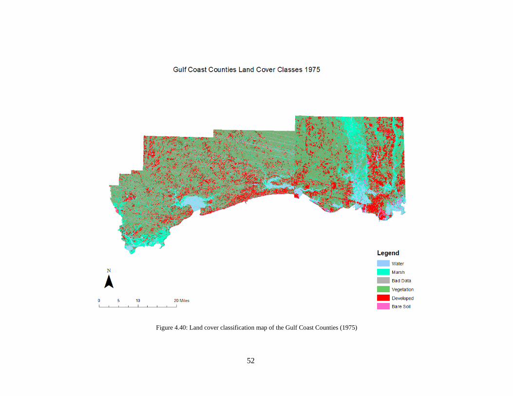
52
Figure 4.40: Land cover classification map of the Gulf Coast Counties (1975)
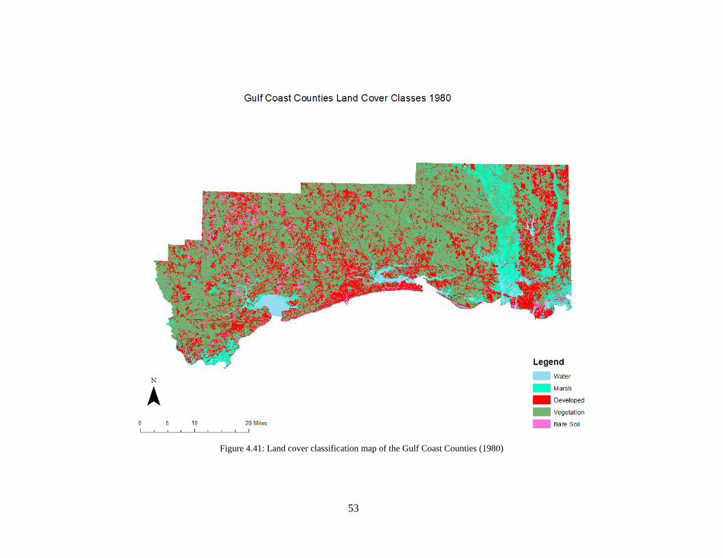
53
Figure 4.41: Land cover classification map of the Gulf Coast Counties (1980)
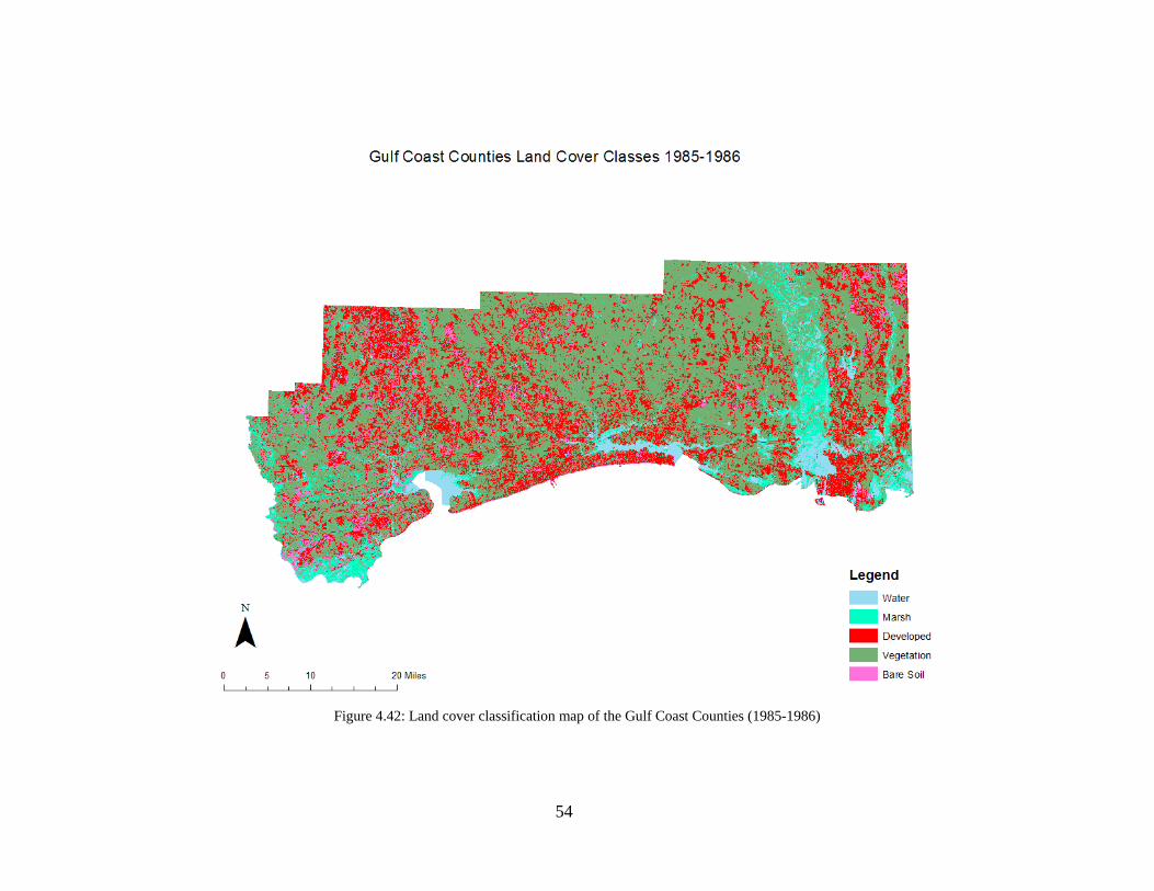
54
Figure 4.42: Land cover classification map of the Gulf Coast Counties (1985-1986)

55
Figure 4.43: Land cover classification map of the Gulf Coast Counties (1990)
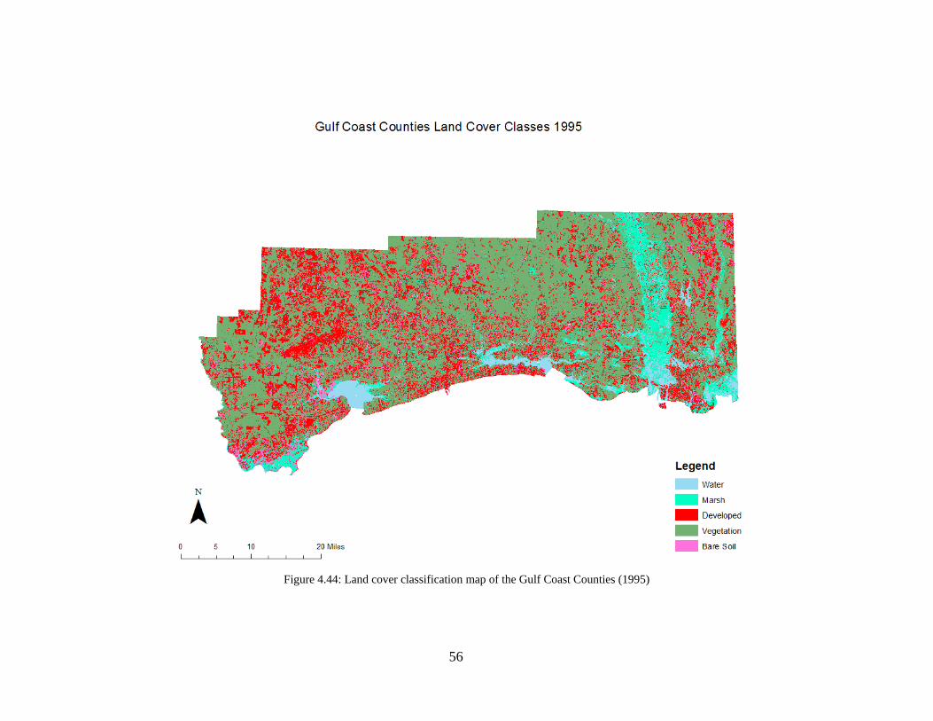
56
Figure 4.44: Land cover classification map of the Gulf Coast Counties (1995)

57
Figure 4.45: Land cover classification map of the Gulf Coast Counties (2000) (1st Classification)
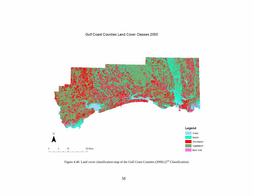
58
Figure 4.46: Land cover classification map of the Gulf Coast Counties (2000) (2nd Classification)
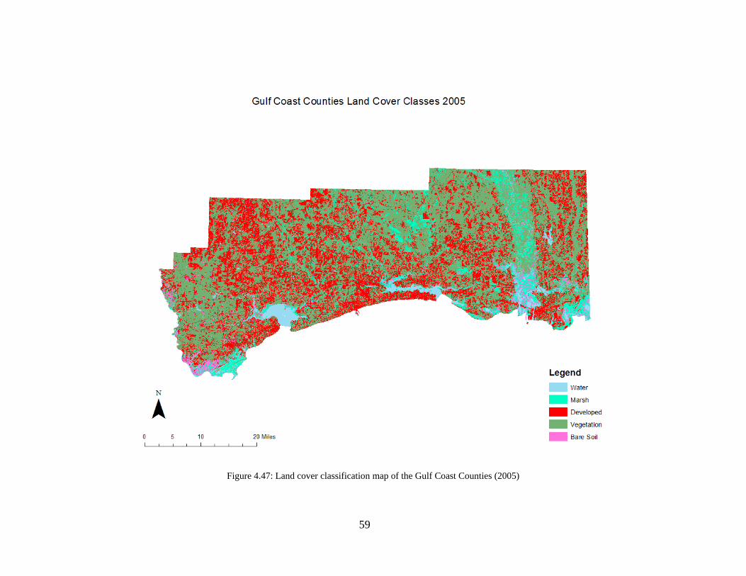
59
Figure 4.47: Land cover classification map of the Gulf Coast Counties (2005)
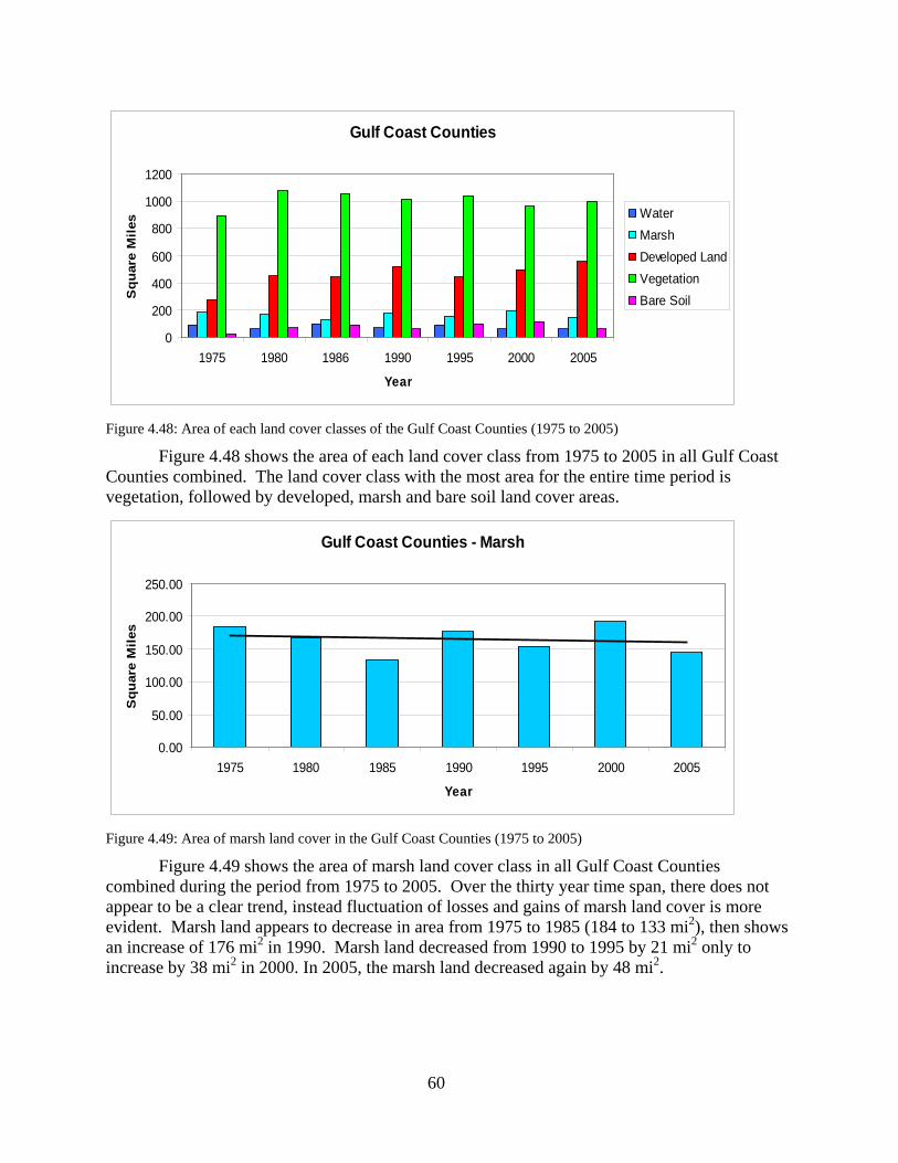
60
Gulf Coast Counties
0
200
400
600
800
1000
1200
1975 1980 1986 1990 1995 2000 2005
Year
Squ
are
Mile
s Water MarshDeveloped LandVegetationBare Soil
Figure 4.48: Area of each land cover classes of the Gulf Coast Counties (1975 to 2005)
Figure 4.48 shows the area of each land cover class from 1975 to 2005 in all Gulf Coast Counties combined. The land cover class with the most area for the entire time period is vegetation, followed by developed, marsh and bare soil land cover areas.
Gulf Coast Counties - Marsh
0.00
50.00
100.00
150.00
200.00
250.00
1975 1980 1985 1990 1995 2000 2005
Year
Squ
are
Mile
s
Figure 4.49: Area of marsh land cover in the Gulf Coast Counties (1975 to 2005)
Figure 4.49 shows the area of marsh land cover class in all Gulf Coast Counties combined during the period from 1975 to 2005. Over the thirty year time span, there does not appear to be a clear trend, instead fluctuation of losses and gains of marsh land cover is more evident. Marsh land appears to decrease in area from 1975 to 1985 (184 to 133 mi2), then shows an increase of 176 mi2 in 1990. Marsh land decreased from 1990 to 1995 by 21 mi2 only to increase by 38 mi2 in 2000. In 2005, the marsh land decreased again by 48 mi2.
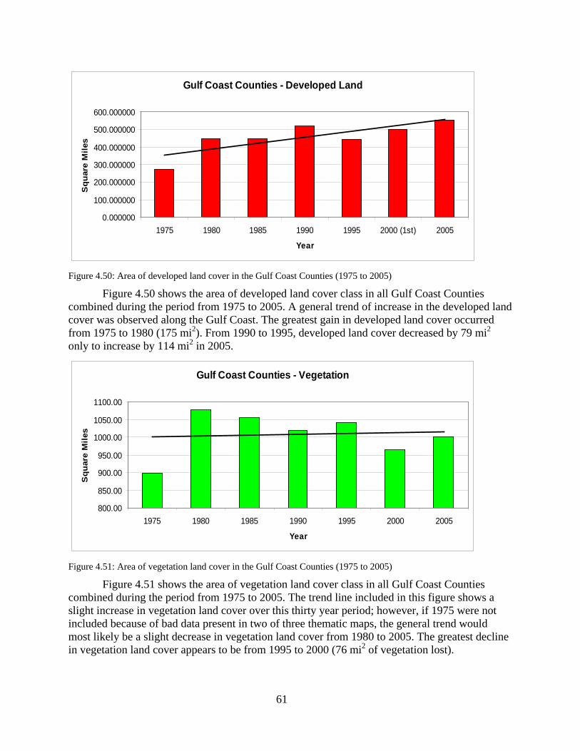
61
Gulf Coast Counties - Developed Land
0.000000
100.000000
200.000000
300.000000
400.000000
500.000000
600.000000
1975 1980 1985 1990 1995 2000 (1st) 2005
Year
Squ
are
Mile
s
Figure 4.50: Area of developed land cover in the Gulf Coast Counties (1975 to 2005)
Figure 4.50 shows the area of developed land cover class in all Gulf Coast Counties combined during the period from 1975 to 2005. A general trend of increase in the developed land cover was observed along the Gulf Coast. The greatest gain in developed land cover occurred from 1975 to 1980 (175 mi2). From 1990 to 1995, developed land cover decreased by 79 mi2 only to increase by 114 mi2 in 2005.
Gulf Coast Counties - Vegetation
800.00
850.00
900.00
950.00
1000.00
1050.00
1100.00
1975 1980 1985 1990 1995 2000 2005
Year
Squ
are
Mile
s
Figure 4.51: Area of vegetation land cover in the Gulf Coast Counties (1975 to 2005)
Figure 4.51 shows the area of vegetation land cover class in all Gulf Coast Counties combined during the period from 1975 to 2005. The trend line included in this figure shows a slight increase in vegetation land cover over this thirty year period; however, if 1975 were not included because of bad data present in two of three thematic maps, the general trend would most likely be a slight decrease in vegetation land cover from 1980 to 2005. The greatest decline in vegetation land cover appears to be from 1995 to 2000 (76 mi2 of vegetation lost).
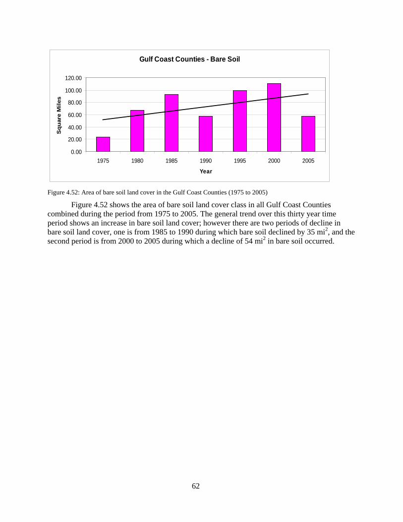
62
Gulf Coast Counties - Bare Soil
0.00
20.00
40.00
60.00
80.00
100.00
120.00
1975 1980 1985 1990 1995 2000 2005
Year
Squ
are
Mile
s
Figure 4.52: Area of bare soil land cover in the Gulf Coast Counties (1975 to 2005)
Figure 4.52 shows the area of bare soil land cover class in all Gulf Coast Counties combined during the period from 1975 to 2005. The general trend over this thirty year time period shows an increase in bare soil land cover; however there are two periods of decline in bare soil land cover, one is from 1985 to 1990 during which bare soil declined by 35 mi2, and the second period is from 2000 to 2005 during which a decline of 54 mi2 in bare soil occurred.
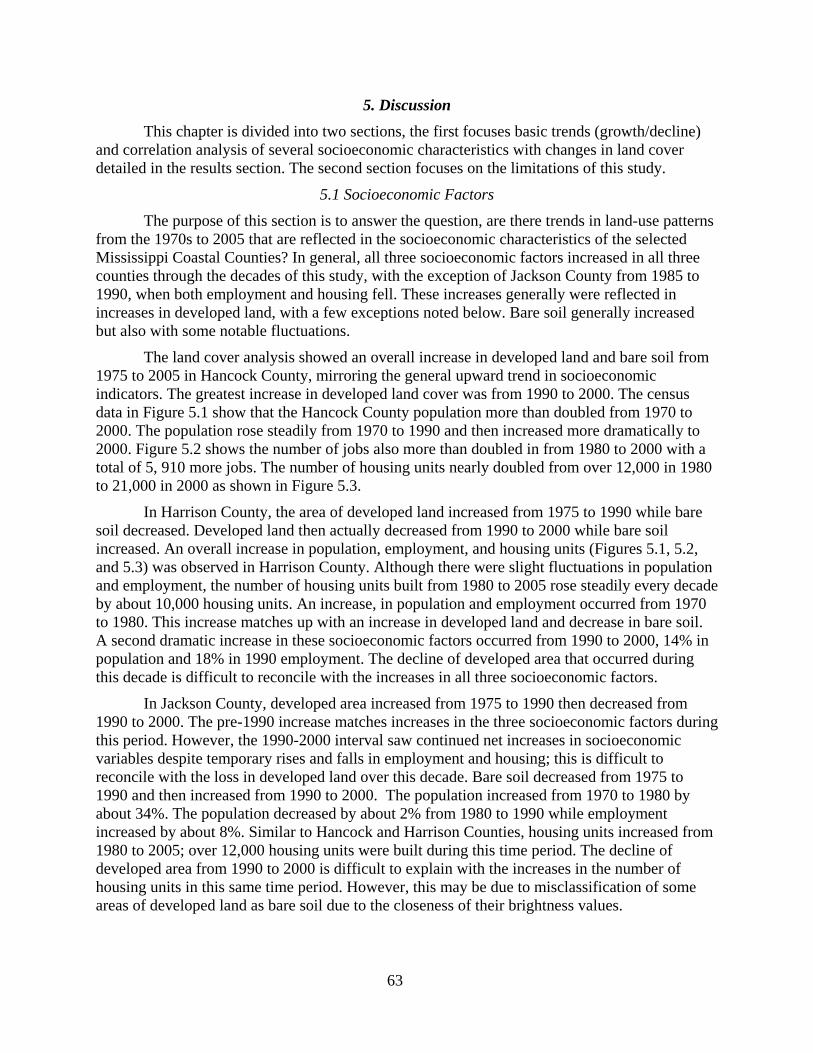
63
5. Discussion This chapter is divided into two sections, the first focuses basic trends (growth/decline)
and correlation analysis of several socioeconomic characteristics with changes in land cover detailed in the results section. The second section focuses on the limitations of this study.
5.1 Socioeconomic Factors The purpose of this section is to answer the question, are there trends in land-use patterns
from the 1970s to 2005 that are reflected in the socioeconomic characteristics of the selected Mississippi Coastal Counties? In general, all three socioeconomic factors increased in all three counties through the decades of this study, with the exception of Jackson County from 1985 to 1990, when both employment and housing fell. These increases generally were reflected in increases in developed land, with a few exceptions noted below. Bare soil generally increased but also with some notable fluctuations.
The land cover analysis showed an overall increase in developed land and bare soil from 1975 to 2005 in Hancock County, mirroring the general upward trend in socioeconomic indicators. The greatest increase in developed land cover was from 1990 to 2000. The census data in Figure 5.1 show that the Hancock County population more than doubled from 1970 to 2000. The population rose steadily from 1970 to 1990 and then increased more dramatically to 2000. Figure 5.2 shows the number of jobs also more than doubled in from 1980 to 2000 with a total of 5, 910 more jobs. The number of housing units nearly doubled from over 12,000 in 1980 to 21,000 in 2000 as shown in Figure 5.3.
In Harrison County, the area of developed land increased from 1975 to 1990 while bare soil decreased. Developed land then actually decreased from 1990 to 2000 while bare soil increased. An overall increase in population, employment, and housing units (Figures 5.1, 5.2, and 5.3) was observed in Harrison County. Although there were slight fluctuations in population and employment, the number of housing units built from 1980 to 2005 rose steadily every decade by about 10,000 housing units. An increase, in population and employment occurred from 1970 to 1980. This increase matches up with an increase in developed land and decrease in bare soil. A second dramatic increase in these socioeconomic factors occurred from 1990 to 2000, 14% in population and 18% in 1990 employment. The decline of developed area that occurred during this decade is difficult to reconcile with the increases in all three socioeconomic factors.
In Jackson County, developed area increased from 1975 to 1990 then decreased from 1990 to 2000. The pre-1990 increase matches increases in the three socioeconomic factors during this period. However, the 1990-2000 interval saw continued net increases in socioeconomic variables despite temporary rises and falls in employment and housing; this is difficult to reconcile with the loss in developed land over this decade. Bare soil decreased from 1975 to 1990 and then increased from 1990 to 2000. The population increased from 1970 to 1980 by about 34%. The population decreased by about 2% from 1980 to 1990 while employment increased by about 8%. Similar to Hancock and Harrison Counties, housing units increased from 1980 to 2005; over 12,000 housing units were built during this time period. The decline of developed area from 1990 to 2000 is difficult to explain with the increases in the number of housing units in this same time period. However, this may be due to misclassification of some areas of developed land as bare soil due to the closeness of their brightness values.
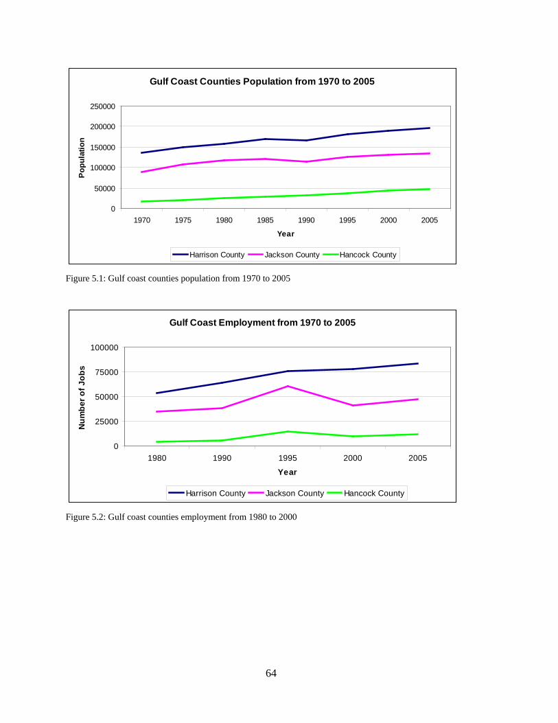
64
Gulf Coast Counties Population from 1970 to 2005
0
50000
100000
150000
200000
250000
1970 1975 1980 1985 1990 1995 2000 2005
Year
Popu
latio
n
Harrison County Jackson County Hancock County
Figure 5.1: Gulf coast counties population from 1970 to 2005
Gulf Coast Employment from 1970 to 2005
0
25000
50000
75000
100000
1980 1990 1995 2000 2005
Year
Num
ber o
f Job
s
Harrison County Jackson County Hancock County
Figure 5.2: Gulf coast counties employment from 1980 to 2000

65
Gulf Coast Housing Units from 1980 to 2005
0
25000
50000
75000
100000
1980 1990 2000 2005
Year
Num
ber o
f Hou
sing
Uni
ts
Harrison County Jackson County Hancock County
Figure 5.3: Gulf coast counties housing units from 1980 to 2005
Table 5.1 shows correlation coefficient of each LULC type with population, employment and housing unit data. These results are not statistically significant because the number of data points is very small. Associations between developed land and socioeconomic factors are generally less evident at the shorter time intervals used in this portion of the analysis than in the analysis of ≥ 10 year intervals presented above. Only a few land cover types and socioeconomic factors showed a strong positive relationship (values near or above 0.8) in Hancock County. These strong positive relationships were between developed land and population, and developed land and housing units. A strong negative correlation was found in Hancock County between vegetation and housing units. The socioeconomic factors did not have any strong relationships with the LULC classes in either Harrison or Jackson counties. Weak positive relationships (> 0.6) were found in Harrison County between developed land and population, marsh and population, and marsh and housing units. Weak negative relationships were found between housing units and vegetation. A weak positive relationship was found in Jackson County between bare soil and population. Table 5.1: Gulf Coast County Socioeconomic Factors and Area of each LULC Class Correlation Coefficients
County Class Correlation Population Employment Housing Units
Hancock
Developed 0.9350 0.7105 0.9024 Marsh -0.6943 -0.5834 -0.5976 Vegetation -0.1869 -0.7300 -0.8271 Bare Soil 0.3484 0.6298 0.1518
Harrison
Developed 0.6285 0.1816 0.4781 Marsh 0.6662 0.6234 0.6691 Vegetation -0.1798 -0.5596 -0.6529 Bare Soil 0.5150 0.1737 0.0596
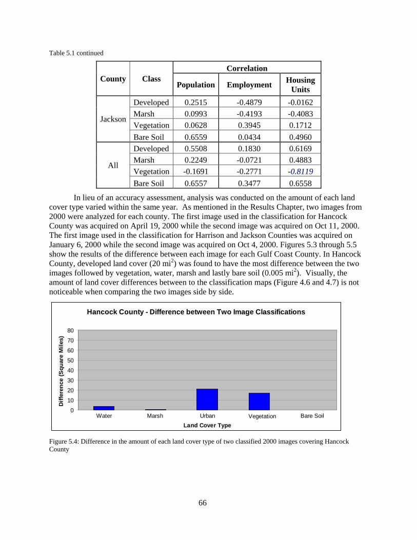
66
Table 5.1 continued
County Class Correlation
Population Employment Housing Units
Jackson
Developed 0.2515 -0.4879 -0.0162 Marsh 0.0993 -0.4193 -0.4083 Vegetation 0.0628 0.3945 0.1712 Bare Soil 0.6559 0.0434 0.4960
All
Developed 0.5508 0.1830 0.6169 Marsh 0.2249 -0.0721 0.4883 Vegetation -0.1691 -0.2771 -0.8119 Bare Soil 0.6557 0.3477 0.6558
In lieu of an accuracy assessment, analysis was conducted on the amount of each land cover type varied within the same year. As mentioned in the Results Chapter, two images from 2000 were analyzed for each county. The first image used in the classification for Hancock County was acquired on April 19, 2000 while the second image was acquired on Oct 11, 2000. The first image used in the classification for Harrison and Jackson Counties was acquired on January 6, 2000 while the second image was acquired on Oct 4, 2000. Figures 5.3 through 5.5 show the results of the difference between each image for each Gulf Coast County. In Hancock County, developed land cover (20 mi2) was found to have the most difference between the two images followed by vegetation, water, marsh and lastly bare soil (0.005 mi2). Visually, the amount of land cover differences between to the classification maps (Figure 4.6 and 4.7) is not noticeable when comparing the two images side by side.
Hancock County - Difference between Two Image Classifications
Water Marsh Urban Vegetation Bare Soil0
10
20
30
40
50
60
70
80
Land Cover Type
Diff
eren
ce (S
quar
e M
iles)
Figure 5.4: Difference in the amount of each land cover type of two classified 2000 images covering Hancock County
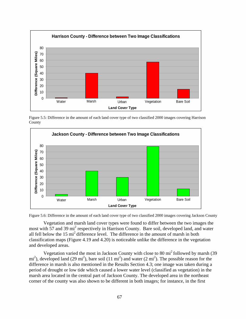
67
Harrison County - Difference between Two Image Classifications
Water Marsh Urban Vegetation Bare Soil0
10
20
30
40
50
60
70
80
Land Cover Type
Diff
eren
ce (S
quar
e M
iles)
Figure 5.5: Difference in the amount of each land cover type of two classified 2000 images covering Harrison County
Jackson County - Difference between Two Image Classifications
Bare SoilVegetationUrbanMarshWater 0
10
20
30
40
50
60
70
80
Land Cover Type
Diff
eren
ce (S
quar
e M
iles)
Figure 5.6: Difference in the amount of each land cover type of two classified 2000 images covering Jackson County
Vegetation and marsh land cover types were found to differ between the two images the most with 57 and 39 mi2 respectively in Harrison County. Bare soil, developed land, and water all fell below the 15 mi2 difference level. The difference in the amount of marsh in both classification maps (Figure 4.19 and 4.20) is noticeable unlike the difference in the vegetation and developed areas.
Vegetation varied the most in Jackson County with close to 80 mi2 followed by marsh (39 mi2), developed land (29 mi2), bare soil (11 mi2) and water (2 mi2). The possible reason for the difference in marsh is also mentioned in the Results Section 4.3; one image was taken during a period of drought or low tide which caused a lower water level (classified as vegetation) in the marsh area located in the central part of Jackson County. The developed area in the northeast corner of the county was also shown to be different in both images; for instance, in the first
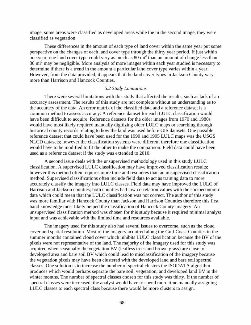
68
image, some areas were classified as developed areas while the in the second image, they were classified as vegetation.
These differences in the amount of each type of land cover within the same year put some perspective on the changes of each land cover type through the thirty year period. If just within one year, one land cover type could very as much as 80 mi2 than an amount of change less than 80 mi2 may be negligible. More analysis of more images within each year studied is necessary to determine if there is a trend in the amount a particular land cover type varies within a year. However, from the data provided, it appears that the land cover types in Jackson County vary more than Harrison and Hancock Counties.
5.2 Study Limitations There were several limitations with this study that affected the results, such as lack of an
accuracy assessment. The results of this study are not complete without an understanding as to the accuracy of the data. An error matrix of the classified data and a reference dataset is a common method to assess accuracy. A reference dataset for each LULC classification would have been difficult to acquire. Reference datasets for the older images from 1970 and 1980s would have most likely required manually digitizing older LULC maps or searching through historical county records relating to how the land was used before GIS datasets. One possible reference dataset that could have been used for the 1990 and 1995 LULC maps was the USGS NLCD datasets; however the classification systems were different therefore one classification would have to be modified to fit the other to make the comparison. Field data could have been used as a reference dataset if the study was extended to 2010.
A second issue deals with the unsupervised methodology used in this study LULC classification. A supervised LULC classification may have improved classification results; however this method often requires more time and resources than an unsupervised classification method. Supervised classifications often include field data to act as training data to more accurately classify the imagery into LULC classes. Field data may have improved the LULC of Harrison and Jackson counties; both counties had low correlation values with the socioeconomic data which could mean that the LULC classification was not correct. The author of this study was more familiar with Hancock County than Jackson and Harrison Counties therefore this first hand knowledge most likely helped the classification of Hancock County imagery. An unsupervised classification method was chosen for this study because it required minimal analyst input and was achievable with the limited time and resources available.
The imagery used for this study also had several issues to overcome, such as the cloud cover and spatial resolution. Most of the imagery acquired along the Gulf Coast Counties in the summer months contained cloud cover which inhibits LULC classification because the BV of the pixels were not representative of the land. The majority of the imagery used for this study was acquired when seasonally the vegetation BV (leafless trees and brown grass) are close to developed area and bare soil BV which could lead to misclassification of the imagery because the vegetation pixels may have been clustered with the developed land and bare soil spectral classes. One solution is to increase the number of spectral clusters the ISODATA algorithm produces which would perhaps separate the bare soil, vegetation, and developed land BV in the winter months. The number of spectral classes chosen for this study was thirty. If the number of spectral classes were increased, the analyst would have to spend more time manually assigning LULC classes to each spectral class because there would be more clusters to assign.
69
Higher resolution imagery may have improved the results of this study as well. The spatial resolution of Landsat imagery (30 m) also may have led to mixed pixel classification errors. Mixed pixels are an issue fore non-homogenous landscapes when the size of the pixel is large enough that it covers an area that has more than one land cover type. Mixed pixels can lead to classification errors since the more abundant brightness value wins out and the less abundant land cover is not represented. The scale of the classification system can account for this issue. The classification used for this study, vegetation, developed land, water and etc was appropriate for the spatial resolution of the Landsat Imagery. Higher resolution imagery requires larger storage space, more processing power (more pixels to classify) and more images are required to cover the three counties used in this study.
70
6.0 Conclusions LULC analysis throughout the Mississippi Gulf Coast Counties over thirty years provides
an interesting look at the temporal changes in the landscape. These results correlated with socioeconomic data show the affects of growth in population, jobs and housing units on the environment. Two Landsat path/row images were found to cover the Gulf Coast Counties. Sixteen images were used in this study, one image per year from 1975 to 2005. After running an ISODATA clustering algorithm, classification of these images into five types of land cover, developed land, vegetation, marsh, water, and bare soil, was completed. The land cover types were then compared by analyzing the area of each type and theirs changes over thirty years. The thematic maps of each county were created to show where the major areas of transition of the environment were located, i.e. from vegetation to developed land and marsh to vegetation in five year intervals.
A literature review of relevant LULC classification studies was conducted. These studies provided insight into various methods and the presentation of the results of classifying land cover in coastal settings. Various types of both supervised and unsupervised methods were described as well as accuracy assessments. Most LULC studies presented results in the form of thematic maps and tables of areas of each LULC type. It was interesting to note that most studies used a different LULC classification system.
Analysis of two sets of images acquired in different seasons of 2000 was conducted to get an idea of the differences of each land cover type within the same year. Each land cover type was found to vary from image to image, in varying degrees. This difference between the areas of each land cover type over this study period is most likely due to the seasonal variations of vegetation from spring to winter to fall. These differences helped put the amount of change of land cover type discussed in the Results Chapter within the thirty year period in perspective; for instance, if the area of vegetation can vary by 80 mi2 within one year than a change less than that in five years is not significant.
Over the past thirty years, the population, employment and housing units in each of the selected coastal counties grew more than most counties in Mississippi. Although, no significant statistical conclusions were drawn from this study (too few data points); developed land and bare soil appeared to be positively correlated to the selected socioeconomic characteristics of Hancock County. Vegetation appeared to be negatively correlated to employment and housing units in Hancock County. These results and the thematic maps suggest that changes in areas of developed land, vegetation, and bare soil could relate to the increases in population, employment, and housing sector in the counties covered by the study. Several limitations were discussed such as an accuracy assessment, unsupervised classification, cloudy imagery and mixed pixels.
71
7.0 References Anderson, J.R., Hardy, E.E., Roach, J.T., Witmer, R.E., 1976. “A Land Use and Land Cover Classification System for Use with Remote Sensor Data,” USGS Professional Paper, Washington D.C., pp.41.
Brown, D., Johnson, K., Loveland, T., and Theobald, D., 2005. “Rural land-use trends in the conterminous United States, 1950-2000,” Ecological Applications, 15:6, pp. 1851-1863.
Bureau of Labor Statistics, 1995. Labor Force Data by County, “1995 Annual Averages,” http://www.bls.gov/lau/tables.htm.
Campbell, D.J., Lusch, D.P., Smucker, T.A., and Wangui, E.E., 2005. “Multiple Methods in the Study of Driving Forces of Land Use and Land Cover Change: A Case Study of SE Kajiado District, Kenya,” Human Ecology, 33:6, pp.763-794.
Carreno, M., Esteve, M., Martinez, J., Palazon, J., and Pardo, M., 2007. “Habitat changes in coastal wetlands associated to hydrological changes in the watershed,” Estuarine, Coastal and Shelf Science, 77, pp. 475-483.
Collins, C. A., Wilkinson, D. W. and Evans, D. L., 2005, “Multi-temporal Analysis of Landsat Data to Determine Forest Age Classes for the Mississippi Statewide Forest Inventory—Preliminary Results,”Proceedings of the Third International Workshop on the Analysis of Multi-Temporal Remote Sensing Images, Biloxi, MS (CD-ROM).
Cowardin, L.M., Carter, V., Golet, F.C., and LaRoe, E.T., 1979, “Classification of wetlands and deepwater habitats of the United States: U.S. Fish and Wildlife Service,” Washington D.C., pp. 103.
Everitt, J., Yang, C., Sriharan, S., and Judd, F., 2008. “Using High Resolution Satellite Imagery to Map Black Mangrove on the Texas Gulf Coast,” J. of Coastal Research, 24:6, pp. 1582-1586.
Gourmelon, F., Bioret, F., and Le Berre, I., 2001. “Land-use changes and implications for management of a small protected island off the coast of Bretagne,” J. of Coastal Convservation, 7, pp. 41-48.
Hanamgond, P., and Mitra, D., 2008. “Evolution of Malvan Coast, Konkan, West Coast of India—A Case Study Using Remote Sensing Data,” J. of Coastal Research, 24:3, pp. 672-678.
Hilbert, K., 2006. “Land Cover Change within the Grand Bay National Estuarine Research Reserve: 1974-2001.” J. of the Coastal Research, 22:6, pp.1552-1557.
Huang, M., Shi, Z., and Gong, J., 2008. “Potential of Multitemporal ERS-2 SAR Imagery for Land Use Mapping in Coastal Zone of Shangyu City, China,” J. Coastal Research, 24:1, pp. 170-176.
Jenson, J.R., 2005, Introductory Digital Image Processing A Remote Sensing Processing. Prentice Hall, 3rd ed. NJ, pp. 457.
Kandus, P., Karszenbaum, and L. Frulla., 1999. “Land cover Classification System for the Lower Delta of the Parana River (Argentina): Its Relationship with Landsat Thematic Mapper Spectral Classes,” J. of Coastal Research, 18:4, pp. 909-926.
72
Klemas, V.V, Dobson, J.E., Ferguson, R.L., and Haddad, K.D., 1993. “A Coastal Land Cover Classification System for the NOAA Coast watch Change Analysis Project,” J. of Coastal Research, 9:3, pp. 862-872.
Lillesand, T. M., Kiefer, R. W., and Chipman, J.W., 2008. Remote sensing and image interpretation. John Wiley & Sons, Inc. USA., pp.221, 400-401, 756.
Oivanki, S.M., Meyer-Arendt, K.J., and Yassin, B., 1995. “Analysis of Land Use and Land Cover Changes on the Mississippi Coast: 1950s to 1992,” Gulf Coast Association of Geological Societies Transactions, 45, pp. 467-473. O’Hara, C.G., King, J.S., Cartwright, J.H., and King, R.L., 2003. “Multi-temporal Land Use and Land Cover Classification of Urbanized Areas within Sensitive Coastal Environments,” IEE Transactions of Geoscience and Remote Sensing, 41, pp. 2005 – 2014.
Qi, S. and Luo, F., 2008. “Land use Change and Environmental Hazard in the Coastal Areas: The Case of Laizhou Gulf, China,” J. of the Coastal Research. 24:5, pp. 1189-1193.
Ramsey III, E.W., Nelson, G.A., and Sapkota, S.K., 2001. “Coastal Change Analysis Program Implemented in Louisiana,” J. of Coastal Research, 17:1, pp. 53-71.
State Data Center, 1992. Center for Population Studies, University of Mississippi, “1990 Census of Population and Housing,” http://www.olemiss.edu/depts/sdc/profiles90.
State Data Center, 2001. Center for Population Studies, University of Mississippi, “2000 Census of Population and Housing,” http://www.olemiss.edu/depts/sdc/census2k.html
U.S. Census Bureau, Center for Economic Studies, 2009. “Local Employment Dynamics,” http://lehd.did.census.gov/led/datatools/qwiapp.html.
U.S. Census Bureau, Geography Division, 2008. “Tiger/Line Shapefiles,” http://www.census.gov/geo/www/tiger/.
U.S. Census, Population Division, 2010. Population Estimates, “Annual Estimates of the Resident Population for Counties of Mississippi: April 1, 2000 to July 1, 2009 (CO-EST2009-01-28),” http://www.census.gov/popest/counties/.
U.S. Dept of Commerce, Bureau of Census, 1982. 1980 Census of Population, “Number of Inhabitants Miss,” http://www.census.gov/prod/www/abs/decennial/1980cenpopv1.html.
Yarbourgh, L.D., Easson, G., and Kuszmaul, J.S., 2005. “Using At-Sensor Radiance and Reflectance Tasseled Cap Transforms Applied to Change Detection for the ASTER Sensor,” IEEE explore. pp.1-5.
Wilkinson, D.W., Parker, R.C., and Evans, D.L., 2008, “Change Detection Techniques for Use in a Statewide Forest Inventory Program,” Photogrammeteric Engineering & Remote Sensing, 74, pp. 893-901.

73
Appendix A The raw socioeconomic data is presented in Table A-1.
Table A-1: Gulf Coast Counties raw socioeconomic data
County Class 2005 2000 1995 1990 1985 1980 1975 1970
Hancock
Population 46088 42967 37802 31760 29091 24537 20000 17387 Employment 11610 10081 14900 5663 N/A 4171 N/A N/A Housing Units 23551 21072 N/A 16561 N/A 12517 N/A N/A
Harrison
Population 195756 189601 181553 165365 168762 157665 149300 134582 Employment 83820 78193 76089 64104 N/A 53337 N/A N/A Housing Units 88138 79636 N/A 67813 N/A 57954 N/A N/A
Jackson
Population 134243 131420 126626 115243 120119 118015 107700 87975 Employment 47500 40990 60691 38119 N/A 35162 N/A N/A Housing Units 56732 51678 N/A 45542 N/A 42635 N/A N/A
74
Vita Ms. Amanda English was born in Daytona, Ohio. Since her father was in the Air Force, she moved around several times throughout her childhood into adolescence; however, today she considers Florida her home. She graduated from Florida Institute of Technology in 2003 with a Bachelor’s degree in Environmental Science. After graduation, she moved to Mississippi to work for the Naval Oceanographic Office as a Physical Scientist in the Mine Warfare Department. After acceptance in the Department of Defense’s Long Term Training Program, she began her graduate studies focusing on Remote Sensing and Coastal Sciences at the University of New Orleans in the fall of 2008. Dr. Mahtab Lodhi provided mentorship over her graduate studies in the Geography Department at UNO until graduation in Spring 2011.