Embed Size (px)
Citation preview

FOR 375 Introduction to Geospatial Analysis for Natural Resource Management Gessler, Spring, 2009
1
Lab #10 Digital Orthophoto Creation (Using Leica Photogrammetry Suite)
References: Leica Photogrammetry Suite Project Manager: Users Guide, Leica Geosystems LLC.
Leica Photogrammetry Suite 9.2
Introduction: The Leica Photogrammetry Suite drastically reduces the cost and time associated with triangulating and
orthorectifying aerial photography, satellite imagery, digital, and video camera imagery when collecting
geographic information. Reliable geographic information can not be collected from raw aerial photography
or satellite imagery due to geometric distortions resulting from various systematic and nonsystematic
errors. These errors occur from camera and sensor orientation, terrain relief, Earth curvature, film and
scanning distortion, and measurement errors. Leica Photogrammetry Suite uses the most reliable geometric
modeling method called the collinearity equation based orthorectification. This process incorporates the
sensor or camera orientation, relief displacement, and the Earth’s curvature in its modeling process.
Orthorectification in Leica Photogrammetry Suite produces planimetrically true orthoimages where all
geometric errors are removed. The orthoimage has the geometric characteristics of a map and the image
qualities of a photograph.
This lab will utilize Leica Photogrammetry Suite to create orthophotos of your aerial photos (EF-I-5, EF-I-
6, and EF-I-7). To create orthophotos with Leica Photogrammetry Suite you must have the following
camera information:
1. Camera Focal Length (mm)
2. Principal Point x offset (mm)
3. Principal Point y offset (mm)
4. Fiducial (x,y) coordinate locations (mm)
5. Average above ground flying height (meters)
This information can be located within the camera calibration report or with the aerial photography/flight
planning report, which can be acquired from the company that flew the project area.
In this lab, you are going to perform the following basic steps:
Create ERDAS IMAGINE (.img) files from scanned aerial photographs in TIFF
format (.tiff)
Create a new Leica Photogrammetry Suite (LPS) project block file
Add imagery to the block file
Define the camera model
Measure ground control points (GCP) and check points
Use the automatic tie point collection function
Triangulate the images
Orthorectify the images
In order to create orthophotos, you must have an aerial photo in digital format. Desktop scanners can be
used to scan film or paper based photographs. Aerial photo film is superior to paper, both in terms of image
detail and geometry. When using a desktop scanner, you should make sure that the active area is at least 9
X 9-inches (i.e., A3 type scanner), enabling you to capture the entire photo frame. An 8.5 X 11-inch
scanner will not capture an entire 9 X 9-inch aerial photograph. LPS utilizes the photo fiducial marks
to define the photo interior orientation.
The required pixel resolution varies depending on the application. Aerial triangulation and feature
collection applications often scan in the 10- to 15-micron range. One micron (micrometer) is equivalent to
1/25400ths of an inch. Orthophoto applications often use 15- to 30-micron pixels. Color film is less sharp
than panchromatic, therefore color ortho applications often use 20- to 40-micron pixels. Table 1 lists the
FOR 375 Introduction to Geospatial Analysis for Natural Resource Management Gessler, Spring, 2009
2
scanning resolutions associated with various scales of photography and image file size. File size is based on
an ERDAS Imagine (.img) format. (NOTE: Files with a .img extension may or may not be an ERDAS
Imagine formatted file. Other .img extensions exist that are not compatible with the ERDAS Imagine
software, i.e., GEM Paint (.img) formatted files.) The ground coverage column refers to the ground
coverage per pixel. Thus, a 1:9600 scale photograph scanned at 16 microns (1588 dpi) has a ground
coverage per pixel of 0.1536 meter by 0.1536 meter. The resulting B/W file size is approximately 84 MB,
assuming a square 9 X 9 inch photograph.
Your school forest photos have been scanned to a TIFF (Tag Image File Format) formatted image file. This
file is formatted to a 400 x 400 pixel per inch image resolution.
Question #1:
Determine the exact ground coverage per pixel of your scanned forest photos. ____________ meters
Question #2:
Convert the scanning resolution from pixels per inch to microns. _____________ microns
Table 1: Scanning Resolutions
FOR 375 Introduction to Geospatial Analysis for Natural Resource Management Gessler, Spring, 2009
3
Viewing a TIFF file in ERDAS IMAGINE
1. Start ERDAS IMAGINE.
2. Click the open layer button within the Viewer that automatically opens when starting ERDAS
IMAGINE.
3. Navigate to C:\FOR_375\Data_files\Orthophoto Generation
4. Next to the Files of type, click on the pull down menu, and select TIFF (*.tiff), select image EF-I-5.
5. Before pressing Enter, select the Raster Options tab at the top of the Select Layer To Add dialog.
6. Under Layers to Colors:, display band 1 in the Red: color gun, band 2 in the Green: color gun, and
band 3 in the Blue: color gun.
7. Click the Fit to Frame check box to fit the image to the current Viewer window size.
8. Click OK to close the Select Layer To Add dialog (click yes if prompted for pyramid layer creation).
Your selected photo image will appear within the viewer. Zoom in on the image by selecting the Zoom In
button located on the Viewer display screen. Click on the image within the Viewer to zoom in. The level
of detail this photo has with a 400 x 400-pixels per inch (PPI) resolution size, and the photos have been
scanned so that north is at the top.
NOTE: Leica Photogrammetry Suite requires scanned images to be in the ERDAS IMAGINE (.img) image
format.
Converting TIFF (.tiff) Image Format to ERDAS IMAGINE (.img) Image Format
Orthophoto Generation
n
FOR 375 Introduction to Geospatial Analysis for Natural Resource Management Gessler, Spring, 2009
4
1. Click on the Import icon on the ERDAS IMAGINE icon panel (bar panel at the top).
The Import button is enabled when the dialog first opens, so that all of the prompts that display in the
dialog are for importing data. When you click on the Export buttons, the prompts change to options for
exporting data.
2. Click on the Type: popup list to select TIFF from the list of available importers.
3. Click on the Media: popup list to select File.
4. Within the Input File (*.tif) window, navigate to
“C:\FOR_375\Data_Files\Orthophoto Generation” and select EF-I-5.tif.
5. Within the Output File (*.img) window, navigate to
“C:\FOR_375\Data_Files\Orthophoto Generation” and name your file EF-I-5.img.
6. In the Import/Export dialog, click OK.
7. The Import TIFF dialog opens:
8. In the Import TIFF dialog window, click Import Options.
FOR 375 Introduction to Geospatial Analysis for Natural Resource Management Gessler, Spring, 2009
5
9. In the Import Options dialog, type 3,2,1 in the Select Layers: selection box.
Since ERDAS Imagine loads the first three bands in the red, green, and blue color guns, importing
the image as 3,2,1 will load the appropriate spectral bands into the proper color guns.
10. Click OK in the Import Options dialog.
11. In the Import TIFF dialog, click OK.
12. When the Job Status dialog indicates Done, click OK to dismiss the Job Status dialog. Your
selected TIFF file has been successfully imported into an ERDAS IMAGINE (.img) formatted
file.
Import the other two TIFF images (6 & 7) into an ERDAS IMAGINE (.img) file format by
repeating the previous steps. Make sure that all your files are being placed in the
“C:\FOR_375\Data_Files\Section_?” directory (replace “?” with your section number (1,2 or 3) .
When you’ve completed importing all the TIFF images to ERDAS IMAGINE (.img) file format,
click Close on the Importing TIFF Data dialog.
Starting the Leica Photogrammetry Suite and Preparing the Block File:
You’re now ready to start the Leica Photogrammetry Suite to create orthophotos.
1. Close all Viewers that are currently open.
2. Select Main | LPS… from the IMAGINE menu bar, or click the Leica Photogrammetry Suite icon on
the ERDAS IMAGINE icon panel.
3.
The LPS Project Manager window opens.
FOR 375 Introduction to Geospatial Analysis for Natural Resource Management Gessler, Spring, 2009
6
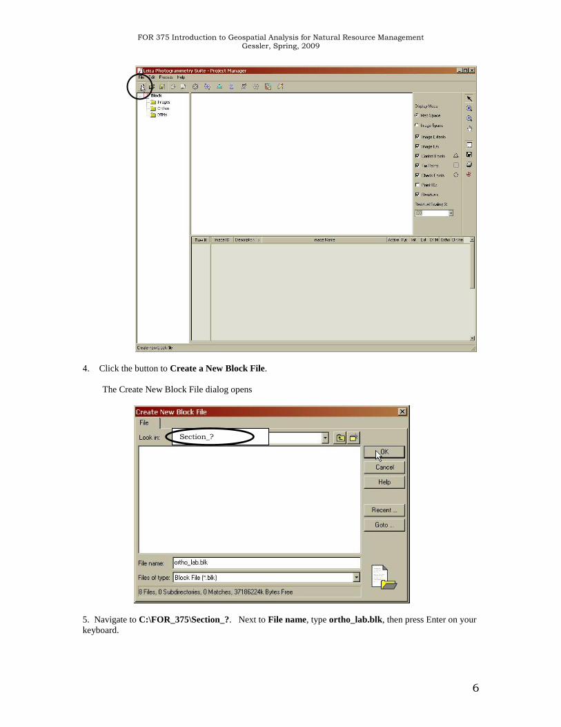
4. Click the button to Create a New Block File.
The Create New Block File dialog opens
5. Navigate to C:\FOR_375\Section_?. Next to File name, type ortho_lab.blk, then press Enter on your
keyboard.
Section_?
FOR 375 Introduction to Geospatial Analysis for Natural Resource Management Gessler, Spring, 2009
7
When you use the Leica Photogrammetry Suite, you create block files. Block files have the .blk
extension. A block file may be made up of only one image, a strip of images that are adjacent to one
another, or several strips of imagery (i.e. “a block”).
The .blk file is a binary file. In it is all the information associated with the block including imagery
locations, camera information, fiducial mark measurements, and GCP measurements.
Click OK to close the Create New Block File dialog. The Model Setup dialog opens.
5. From the Select Geometric Model list, select Frame Camera.
6. Click OK to close the Model Setup dialog.
The Block Property Setup dialog opens.
7. Click the Set Projection button in the Set Reference System section of the Block Property Setup
dialog.
FOR 375 Introduction to Geospatial Analysis for Natural Resource Management Gessler, Spring, 2009
8
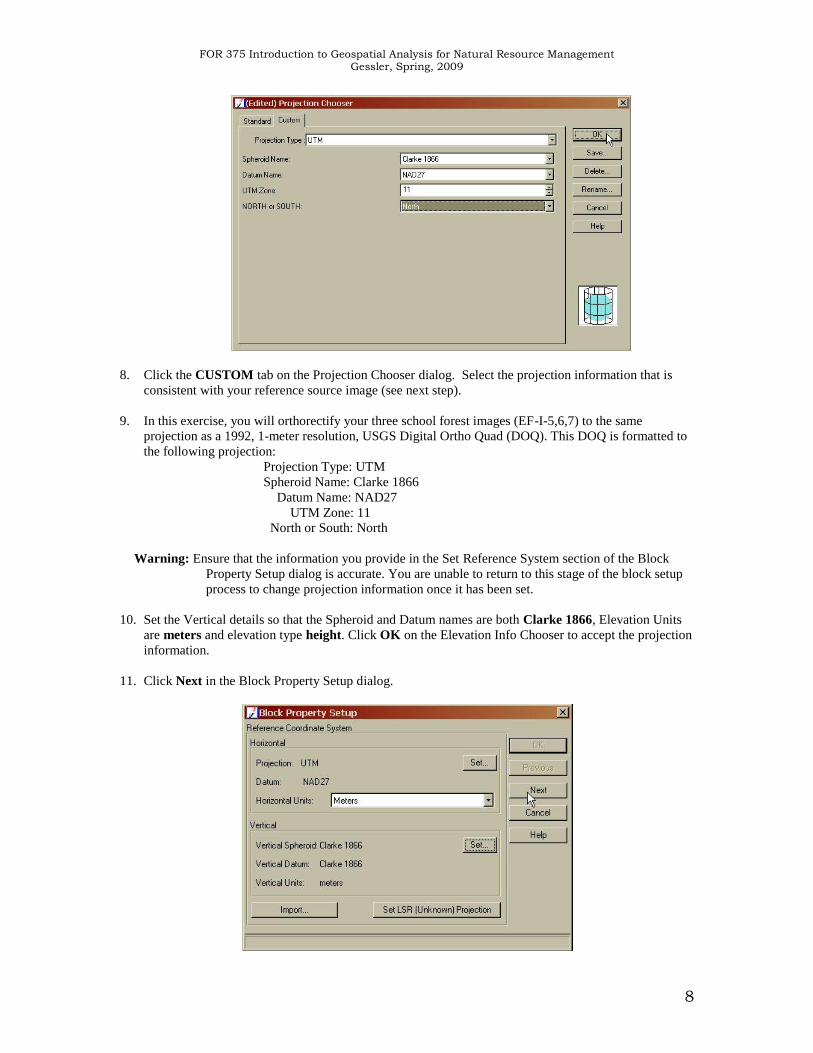
8. Click the CUSTOM tab on the Projection Chooser dialog. Select the projection information that is
consistent with your reference source image (see next step).
9. In this exercise, you will orthorectify your three school forest images (EF-I-5,6,7) to the same
projection as a 1992, 1-meter resolution, USGS Digital Ortho Quad (DOQ). This DOQ is formatted to
the following projection:
Projection Type: UTM
Spheroid Name: Clarke 1866
Datum Name: NAD27
UTM Zone: 11
North or South: North
Warning: Ensure that the information you provide in the Set Reference System section of the Block
Property Setup dialog is accurate. You are unable to return to this stage of the block setup
process to change projection information once it has been set.
10. Set the Vertical details so that the Spheroid and Datum names are both Clarke 1866, Elevation Units
are meters and elevation type height. Click OK on the Elevation Info Chooser to accept the projection
information.
11. Click Next in the Block Property Setup dialog.
FOR 375 Introduction to Geospatial Analysis for Natural Resource Management Gessler, Spring, 2009
9
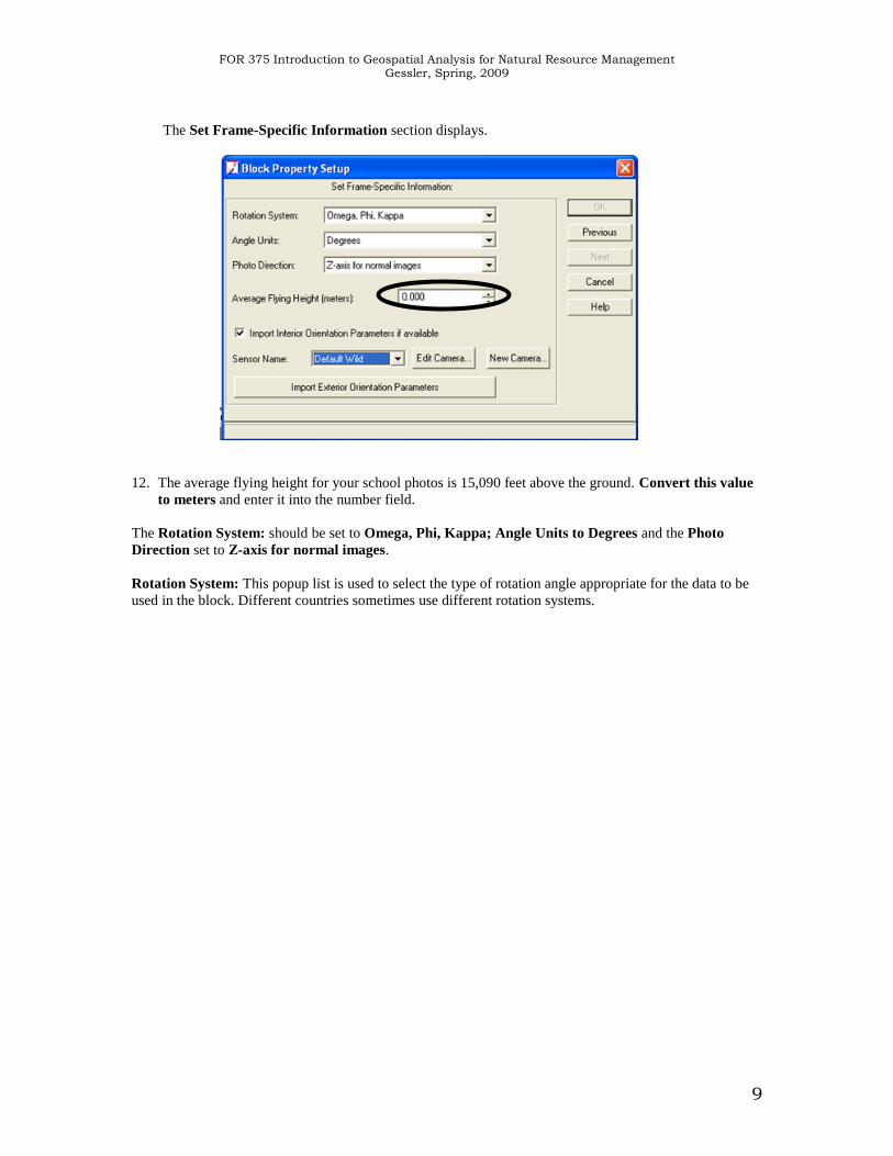
The Set Frame-Specific Information section displays.
12. The average flying height for your school photos is 15,090 feet above the ground. Convert this value
to meters and enter it into the number field.
The Rotation System: should be set to Omega, Phi, Kappa; Angle Units to Degrees and the Photo
Direction set to Z-axis for normal images.
Rotation System: This popup list is used to select the type of rotation angle appropriate for the data to be
used in the block. Different countries sometimes use different rotation systems.
FOR 375 Introduction to Geospatial Analysis for Natural Resource Management Gessler, Spring, 2009
10
Omega, Phi and Kappa define the orientation of the sensor as it existed when the photograph or imagery
was captured. The three rotation angles define the relationship between the axis of the ground system and
the image coordinate system. The rotation angles are used to form a 3 by 3 rotation matrix, which is used
within the aerial triangulation functional model (i.e. block bundle adjustment).
The primary axis is the axis about which the first rotation occurs. Rotation follows the right-hand rule
which says that when the thumb of the right hand points in the positive direction of an axis, the curled
fingers point in the direction of positive rotation for that axis.
Omega, Phi, Kappa: This is the most commonly used convention, recommended by ISPRS.
Omega is a positive rotation around the X-axis; Phi is a positive rotation around the Y-axis;
Kappa is positive rotation around the Z-axis. In this system, X is the primary axis.
Phi(+), Omega, Kappa In this system, which is most commonly used in Germany, Y is the
primary axis. Phi is a positive rotation around the Y-axis; Omega is a positive rotation around the
X-axis; Kappa is a positive rotation around the Z-axis.
Phi(-), Omega, Kappa In this system, which is most commonly used in China, Y is the primary
axis. Phi is a negative rotation around the Y-axis; Omega is positive rotation around the X-axis;
Kappa is a positive rotation around the Z-axis.
Photo Direction: This popup list is used to select the direction appropriate for the data to be used in the
block project.
Z-axis for normal images Select this option if using aerial photography for your block project.
Aerial photographs have the optical axis of the camera directed toward the Z-axis of the ground
coordinate system.
Y-axis for close-range images Select this option when using ground-based photography.
Terrestrial or ground-based photographs have the optical axis of the camera directed toward the Y-
axis of the ground coordinate system.
13. Click OK to close the Block Property Setup dialog.
The main IMAGINE OrthoBASE dialog opens.
FOR 375 Introduction to Geospatial Analysis for Natural Resource Management Gessler, Spring, 2009
11
The main IMAGINE OrthoBASE dialog identifies the images being used in the block file. Each image has
a series of columns associated with it.
The Row # column enables you to select an image specifically for use with Leica Photogrammetry Suite.
For example, you may want to generate pyramid layers for one image alone.
The Image ID column provides a numeric identifier for each image in the block. You can change the
Image ID if you wish.
The > column lets you designate the image that is currently active.
The Image Name column lists the directory path and the file name for each image. When the full path to
the image is specified, the corresponding Online column is green. The Active column displays an X
designating which images are going to be used in the LPS processes such as automatic tie point generation,
triangulation, and orthorectification.
The final six columns’ status is indicated in terms of color: green means the process is complete and
accurate; red means the process is incomplete.
The Pyr. Column indicates the presence of pyramid layers. The Int. column indicates if the fiducial marks
have been measured for interior orientation. The Ext. column indicates if the final exterior orientation
parameters are complete. The DTM column if elevation data has been provided for your control points
The Ortho column indicates if the images have been orthorectified. The Online column indicates if the
images have a specified location.
Adding Imagery to the Block:
Now you’re going to add images to the block file and define the camera model.
1. Select Edit | Add Frame from the LPS menu bar.
FOR 375 Introduction to Geospatial Analysis for Natural Resource Management Gessler, Spring, 2009
12
The Image File Name dialog opens.
2. Navigate to “C:\FOR_375\Section_?” and select EF_i_5.img.
3. Click OK to add the image and close the Image File Name dialog.
The frame image file is loaded into LPS and displayed in the CellArray.
Notice that the Pyr., Int., Ext., DTM, and Ortho column status blocks are colored red. This indicates that
these processes are incomplete. The Online status block is colored green which indicates that the image has
a specified location.
Section_?
FOR 375 Introduction to Geospatial Analysis for Natural Resource Management Gessler, Spring, 2009
13
4. Add the other two photos (ef_i_6 and ef_i_7) to the block file by repeating steps 1 – 3. Click your
save icon to save your block file. You can exit LPS and return at any time now and re-open your
block file. It will return you to the last point you were at before exiting (***it’s a good idea to save
frequently when working***).
Next, you will compute pyramid layers for the images in the block file. Pyramid layers are used to
optimize image display and automatic tie point collection.
Compute Pyramid Layers:
The pyramid is a data structure consisting of the same image represented several times, at a decreasing
spatial resolution each time. Each level of the pyramid contains the image at a particular resolution.
IMAGINE gives you the option to "pyramid" large images for faster processing in the Viewer. This option
creates reduced subsampled raster layers. These can either be stored within the .img HFA file, or as a
separate file with the .rrd extension, determined by Preference settings.
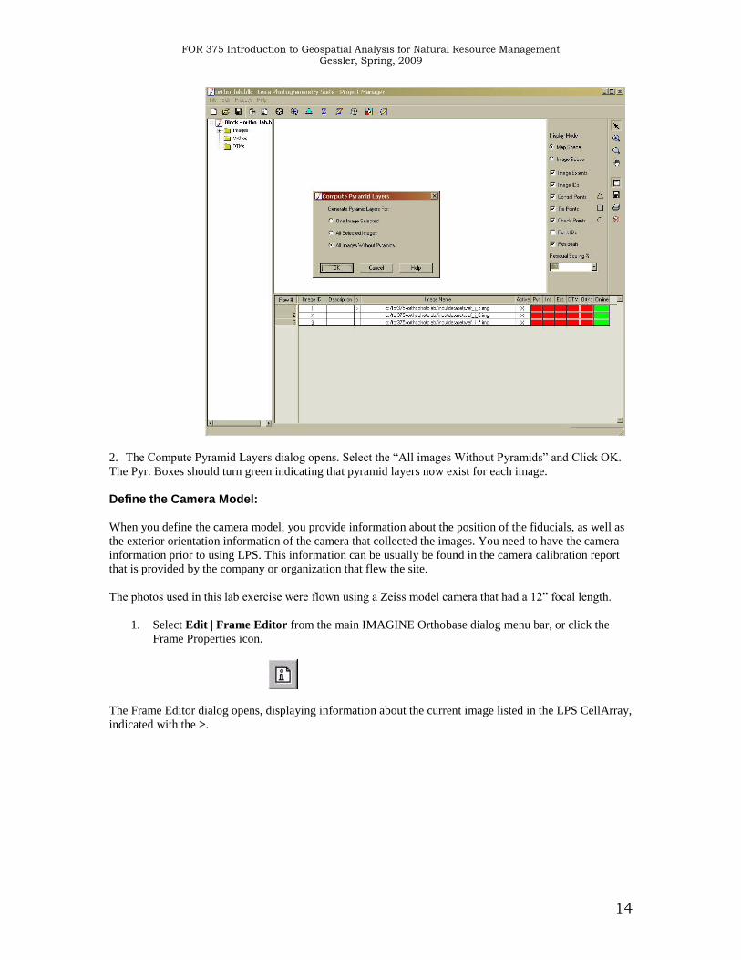
1. Click the Edit menu, and then choose the Compute Pyramid Layers option.
FOR 375 Introduction to Geospatial Analysis for Natural Resource Management Gessler, Spring, 2009
14
2. The Compute Pyramid Layers dialog opens. Select the “All images Without Pyramids” and Click OK.
The Pyr. Boxes should turn green indicating that pyramid layers now exist for each image.
Define the Camera Model:
When you define the camera model, you provide information about the position of the fiducials, as well as
the exterior orientation information of the camera that collected the images. You need to have the camera
information prior to using LPS. This information can be usually be found in the camera calibration report
that is provided by the company or organization that flew the site.
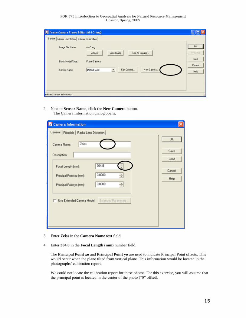
The photos used in this lab exercise were flown using a Zeiss model camera that had a 12” focal length.
1. Select Edit | Frame Editor from the main IMAGINE Orthobase dialog menu bar, or click the
Frame Properties icon.
The Frame Editor dialog opens, displaying information about the current image listed in the LPS CellArray,
indicated with the >.
FOR 375 Introduction to Geospatial Analysis for Natural Resource Management Gessler, Spring, 2009
15
2. Next to Sensor Name, click the New Camera button.
The Camera Information dialog opens.
3. Enter Zeiss in the Camera Name text field.
4. Enter 304.8 in the Focal Length (mm) number field.
The Principal Point xo and Principal Point yo are used to indicate Principal Point offsets. This
would occur when the plane tilted from vertical plane. This information would be located in the
photographs’ calibration report.
We could not locate the calibration report for these photos. For this exercise, you will assume that
the principal point is located in the center of the photo (“0” offset).
FOR 375 Introduction to Geospatial Analysis for Natural Resource Management Gessler, Spring, 2009
16
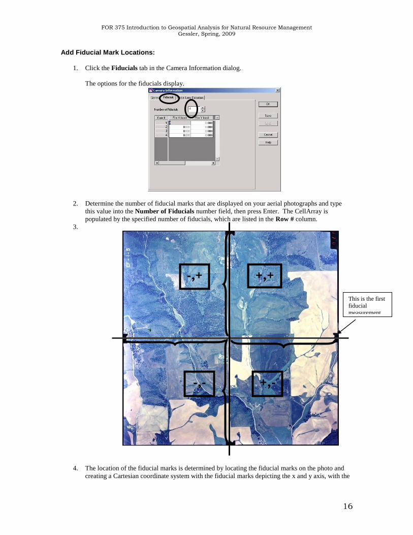
Add Fiducial Mark Locations:
1. Click the Fiducials tab in the Camera Information dialog.
The options for the fiducials display.
2. Determine the number of fiducial marks that are displayed on your aerial photographs and type
this value into the Number of Fiducials number field, then press Enter. The CellArray is
populated by the specified number of fiducials, which are listed in the Row # column.
3.
4. The location of the fiducial marks is determined by locating the fiducial marks on the photo and
creating a Cartesian coordinate system with the fiducial marks depicting the x and y axis, with the
+,+
-,-
-,+
+,-
This is the first
fiducial
measurement.
FOR 375 Introduction to Geospatial Analysis for Natural Resource Management Gessler, Spring, 2009
17
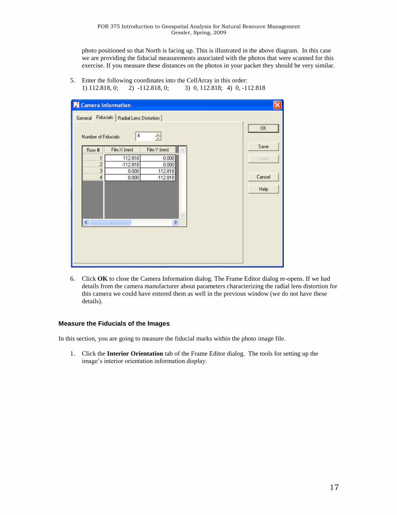
photo positioned so that North is facing up. This is illustrated in the above diagram. In this case
we are providing the fiducial measurements associated with the photos that were scanned for this
exercise. If you measure these distances on the photos in your packet they should be very similar.
5. Enter the following coordinates into the CellArray in this order:
1) 112.818, 0; 2) -112.818, 0; 3) 0, 112.818; 4) 0, -112.818
6. Click OK to close the Camera Information dialog. The Frame Editor dialog re-opens. If we had
details from the camera manufacturer about parameters characterizing the radial lens distortion for
this camera we could have entered them as well in the previous window (we do not have these
details).
Measure the Fiducials of the Images
In this section, you are going to measure the fiducial marks within the photo image file.
1. Click the Interior Orientation tab of the Frame Editor dialog. The tools for setting up the
image’s interior orientation information display.
FOR 375 Introduction to Geospatial Analysis for Natural Resource Management Gessler, Spring, 2009
18
2. Make sure the first Fiducial Orientation icon is selected.
3. Click the Viewer icon.
A Main View opens in the main block file window, with an Overview that shows the entire image and a
Detail View that shows the part of the image within the Link Cursor (small box) of the image. Any of the
three views can be used for measuring the fiducials, however, it is usually easiest to select them in the
Detail View. You can select the box, expand the size or decrease the sizes to change your view, or move
the box. Become familiar with these tools.
The approximate area of the first fiducial is identified by the Link Cursor in the Main View, and displays
in the Detail View.
4. Click in the center of the Link Cursor in the Over View and drag it so that the first fiducial mark
listed in the CellArray (>) is in the center.
5. In the Main View, drag the Link Cursor so that the fiducial mark dot is in the center.
6. Click the Place Image Fiducial icon on the Interior Orientation tab.
Your cursor becomes a crosshair when placed over any one of the views. You want to use your zoom in
tools to place the fiducial cross-hair as precisely as possible. Care in doing these steps will result in less
work and more accurate results.
7. Measure the first fiducial by clicking in its center in the Detail View.
The fiducial point is measured and reported in Image X and Image Y coordinates, and the display
automatically moves to the approximate location of the next fiducial.
FOR 375 Introduction to Geospatial Analysis for Natural Resource Management Gessler, Spring, 2009
19
8. Measure the remaining fiducials using step 5 through step 7. You should notice that as you place a
fiducial location the row for that fiducial mark lists the image coordinates for that point.
When all four fiducials are measured, the display returns to the first fiducial mark.
Your solution (displayed over the Solve button on the Interior Orientation tab of the Frame Editor)
should usually be ½ or less the pixel size of your image. In this case the error will be greater than this, so
try to attain the lowest error possible by remeasuring. To re-measure, click in the row of the Point # you
wish to change, click the Selection tool , then reposition the fiducial mark in the Detail View. You can
improve the positioning of the points by zooming in on the detail view and by changing the image contrast.
Question #3: What is your RMS error for each photo? (Return to this question later to answer for
ef-i-6 and ef-i-7)
_____________________________________________________________________
9. Click on the Viewer icon to dismiss the views.
Main View
Over View
Detail View
Link Cursors
FOR 375 Introduction to Geospatial Analysis for Natural Resource Management Gessler, Spring, 2009
20
Enter Exterior Orientation Information
Exterior Orientation - This tab allows you to specify the exterior orientation parameters for your camera as
they existed at the time of image capture. There are six parameters, with information regarding the status
and standard deviation of each parameter.
Perspective Center (meters) - This set of parameters define the position of the perspective center at the
time of image capture. They may be provided with the data set or they may be determined by LPS.
Rotation Angles(degrees) - This set of parameters define the rotation in degrees of the camera at the time
of image capture. They may be provided with the data set or they may be determined by LPS.
1. Click the Exterior Information tab on the Frame Editor dialog.
Exterior Information could not be obtained for your aerial photographs by reviewing the camera calibration
report. You will have the LPS software determine this information based on a mathematical solution.
2. For all columns in the Exterior Information tab, click the Set Status dropdown list and choose
Unknown.
Now, you need to measure fiducials and define the exterior orientation for the remaining images in
the block file.
3. Click on the Sensor tab in the Frame Editor dialog.
This returns you to the beginning of the process. Now you will complete this process two more
times, once for each remaining image in the block file (ef-i-6, ef-i-7), measuring fiducials and
selecting Unknown for all columns in the exterior information tab.
4. Click the Next button on the Frame Editor dialog.
The Image File Name on the Sensor tab changes to the next image, ef-i-6, in the LPS Cell Array.
FOR 375 Introduction to Geospatial Analysis for Natural Resource Management Gessler, Spring, 2009
21
5. Note that the camera displayed, Zeiss, is the same as that entered for the first image.
6. Follow steps 1-9 in the Measure Fiducials of the Images section and steps 1-3 in the Enter
Exterior Orientation Information section.
7. Click the Next button on the Frame Editor dialog and follow the same procedure as in step 6
above to enter interior and exterior information for photo ef-i-7.
8. Once all information has been entered in the interior and exterior orientation tabs, click OK to
close the Frame Editor dialog. Note that the Int. column of the main IMAGINE OrthoBASE
dialog is green, indicating that the Interior Orientation information has been specified. The
Interior Orientation section of this lab is now complete.
Be sure to SAVE your work by saving in the main block toolbox.
In the following section you will measure ground control points to determine the exterior orientation of
your photos (entered as “Unknowns” above). You will assign a ground coordinate system to your photos
through the placement of ground control points on your photos and on a DOQ that has a known ground
coordinate system. Terrain variations will also be accounted for by using a DEM to determine the
elevation of each control point. See the “Introduction to the Orthophoto generation exercise” for more
details.
FOR 375 Introduction to Geospatial Analysis for Natural Resource Management Gessler, Spring, 2009
22
Measure Ground Control and Check Points (Completing Exterior Orientation):
Now that you have measured the fiducials and provided interior orientation of each image that makes up
the block, you are ready to use the Point Measurement Tool to measure the position of ground control
points and tie points in the images.
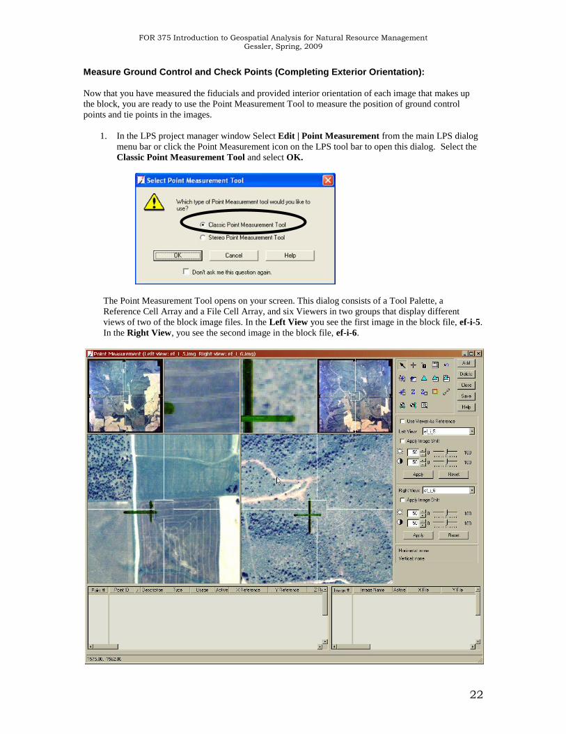
1. In the LPS project manager window Select Edit | Point Measurement from the main LPS dialog
menu bar or click the Point Measurement icon on the LPS tool bar to open this dialog. Select the
Classic Point Measurement Tool and select OK.
The Point Measurement Tool opens on your screen. This dialog consists of a Tool Palette, a
Reference Cell Array and a File Cell Array, and six Viewers in two groups that display different
views of two of the block image files. In the Left View you see the first image in the block file, ef-i-5.
In the Right View, you see the second image in the block file, ef-i-6.
FOR 375 Introduction to Geospatial Analysis for Natural Resource Management Gessler, Spring, 2009
23
For information about the tools contained in the Point Measurement Tool Palette, see the On-Line Help.
Ground Control Points (GCP) are typically placed in areas such as road intersections, building corners, a
large tree, or landmarks. You should avoid placing control points on features that vary, such as forest lines
and water features. Once you have collected some well-distributed GCP’s that are common to two or more
images in the block file, you can perform triangulation, which will rectify the image to remove distortions
relating to camera errors and photo acquisition difficulties. This orthorectification process will then
produce a planimetric image that can be printed to paper and used as a map.
The next series of steps takes you through the process of collecting a GCP. You will rectify your school
photos horizontally by using a digital orthophotoquad (DOQ). DOQs are black and white photos that have
been geographically rectified. To remove vertical distortions from your school photos, you will use a USGS
Digital Elevation Model (DEM).
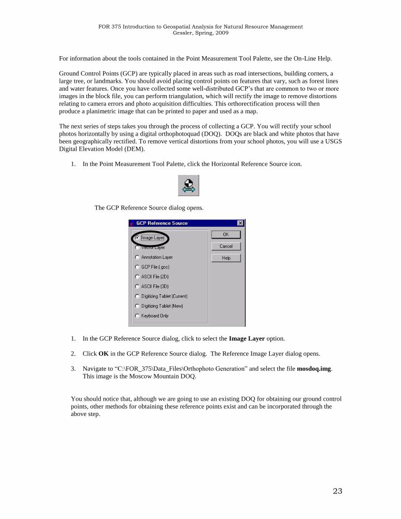
1. In the Point Measurement Tool Palette, click the Horizontal Reference Source icon.
The GCP Reference Source dialog opens.
1. In the GCP Reference Source dialog, click to select the Image Layer option.
2. Click OK in the GCP Reference Source dialog. The Reference Image Layer dialog opens.
3. Navigate to “C:\FOR_375\Data_Files\Orthophoto Generation” and select the file mosdoq.img.
This image is the Moscow Mountain DOQ.
You should notice that, although we are going to use an existing DOQ for obtaining our ground control
points, other methods for obtaining these reference points exist and can be incorporated through the
above step.
FOR 375 Introduction to Geospatial Analysis for Natural Resource Management Gessler, Spring, 2009
24
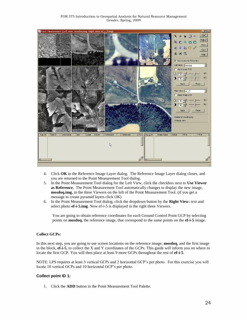
4. Click OK in the Reference Image Layer dialog. The Reference Image Layer dialog closes, and
you are returned to the Point Measurement Tool dialog.
5. In the Point Measurement Tool dialog for the Left View, click the checkbox next to Use Viewer
as Reference. The Point Measurement Tool automatically changes to display the new image,
mosdoq.img, in the three Viewers on the left of the Point Measurement Tool. (if you get a
message to create pyramid layers click OK)
6. In the Point Measurement Tool dialog, click the dropdown button by the Right View: text and
select photo ef-i-5.img. Now ef-i-5 is displayed in the right three Viewers.
You are going to obtain reference coordinates for each Ground Control Point GCP by selecting
points on mosdoq, the reference image, that correspond to the same points on the ef-i-5 image.
Collect GCPs:
In this next step, you are going to use screen locations on the reference image, mosdoq, and the first image
in the block, ef-i-5, to collect the X and Y coordinates of the GCPs. This guide will inform you on where to
locate the first GCP. You will then place at least 9 more GCPs throughout the rest of ef-i-5.
NOTE: LPS requires at least 3 vertical GCPs and 2 horizontal GCP’s per photo. For this exercise you will
locate 10 vertical GCPs and 10 horizontal GCP’s per photo.
Collect point ID 1:
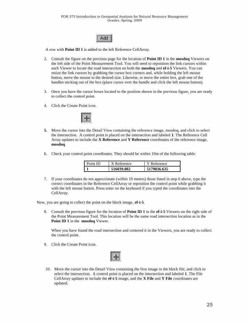
1. Click the ADD button in the Point Measurement Tool Palette.
FOR 375 Introduction to Geospatial Analysis for Natural Resource Management Gessler, Spring, 2009
25
A row with Point ID 1 is added to the left Reference CellArray.
2. Consult the figure on the previous page for the location of Point ID 1 in the mosdoq Viewers on
the left side of the Point Measurement Tool. You will need to reposition the link cursors within
each Viewer to locate the road intersection on both the mosdoq and ef-i-5 Viewers. You can
resize the link cursors by grabbing the cursor box corners and, while holding the left mouse
button, move the mouse to the desired size. Likewise, to move the entire box, grab one of the
handles sticking out of the box (place cursor over the handle and click the left mouse button).
3. Once you have the cursor boxes located to the position shown in the previous figure, you are ready
to collect the control point.
4. Click the Create Point icon.
5. Move the cursor into the Detail View containing the reference image, mosdoq, and click to select
the intersection. A control point is placed on the intersection and labeled 1. The Reference Cell
Array updates to include the X Reference and Y Reference coordinates of the reference image,
mosdoq.
6. Check your control point coordinates. They should be within 10m of the following table:
Point ID X Reference Y Reference
1 516039.882 5179836.635
7. If your coordinates do not approximate (within 10 meters) those listed in step 6 above, type the
correct coordinates in the Reference CellArray or reposition the control point while grabbing it
with the left mouse button. Press enter on the keyboard if you typed the coordinates into the
CellArray.
Now, you are going to collect the point on the block image, ef-i-5.
8. Consult the previous figure for the location of Point ID 1 in the ef-i-5 Viewers on the right side of
the Point Measurement Tool. This location will be the same road intersection location as in the
Point ID 1 in the mosdoq Viewer.
When you have found the road intersection and centered it in the Viewers, you are ready to collect
the control point.
9. Click the Create Point icon.
10. Move the cursor into the Detail View containing the first image in the block file, and click to
select the intersection. A control point is placed on the intersection and labeled 1. The File
CellArray updates to include the ef-i-5 image, and the X File and Y File coordinates are
updated.
FOR 375 Introduction to Geospatial Analysis for Natural Resource Management Gessler, Spring, 2009
26
11. Check your control point coordinates. They should approximate those in the following table:
Image Name X File Y File
ef-i-5 1652.884 2508.484
12. If your coordinates do not approximate (within six pixels) those listed in step 11 above, type the
correct coordinates in the Reference CellArray or reposition the control point while grabbing it
with the left mouse button. Press enter on the keyboard if you typed the coordinates into the
CellArray.
Collect point ID 2 – 10:
1. Follow steps 1 – 12 ( in the collect Point ID 1 section) to collect 9 more GCPs. Choose your points
with care. Spread the points out so that they are not located in the same area. Where does most of
the distortion fall within an air photo? These are areas that you will need to place a GCP so that
the photo can be shifted and repositioned into its proper spatial location.
Your Moscow Mountain DOQ was captured in 1992. What year were your air photos taken? This
will cause some difficulties in finding distinguishable points in both the reference image and the
block file image. Choose road intersections, buildings, and other well-defined features for you
GCPs. *** It would be smart to mark all your GCP’s with its corresponding point number on
your air photo (ef-i-5) for future reference. This will also allow you to reference how well you’ve
distributed points around your photo.
NOTE: REMEMBER TO PRESS THE ADD BUTTON TO SELECT THE NEXT GCP,
OTHERWISE YOU WILL MOVE THE PREVIOUS GCP TO A DIFFERENT
LOCATION. This is a COMMON error made during these steps of the lab.
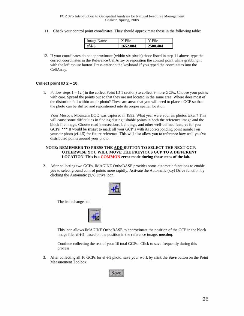
2. After collecting two GCPs, IMAGINE OrthoBASE provides some automatic functions to enable
you to select ground control points more rapidly. Activate the Automatic (x,y) Drive function by
clicking the Automatic (x,y) Drive icon.
The icon changes to:
This icon allows IMAGINE OrthoBASE to approximate the position of the GCP in the block
image file, ef-i-5, based on the position in the reference image, mosdoq.
Continue collecting the rest of your 10 total GCPs. Click to save frequently during this
process.
3. After collecting all 10 GCPs for ef-i-5 photo, save your work by click the Save button on the Point
Measurement Toolbox.
FOR 375 Introduction to Geospatial Analysis for Natural Resource Management Gessler, Spring, 2009
27
Set the Vertical Reference Source:
To provide Z, or elevation values for all of the reference control points you selected in the reference image,
mosdoq, you are going to specify a digital elevation model (DEM), mosdem.img, which contains height
information.
1. Click the Vertical Reference Source icon.
The Vertical Reference Source dialog opens, in which you will select the DEM that is going to supply
height information.
2. Click to Find DEM option.
3. Navigate to “C:\FOR_375\Data_Files\Orthophoto Generation” directory and select the DEM file
mosdem.img.
4. Click OK in the File Chooser dialog. The DEM file you selected is shown in the DEM section of
the Vertical Reference Source dialog.
5. Click OK in the Vertical Reference Source dialog.
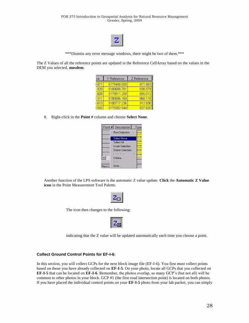
6. Within the Reference CellArray, right-click in the Point # column within the reference CellArray
and select the Select All option.
7. Click on the Update Z Values on Selected Points icon.
FOR 375 Introduction to Geospatial Analysis for Natural Resource Management Gessler, Spring, 2009
28
***Dismiss any error message windows, there might be two of them.***
The Z Values of all the reference points are updated in the Reference CellArray based on the values in the
DEM you selected, mosdem.
8. Right-click in the Point # column and choose Select None.
Another function of the LPS software is the automatic Z value update. Click the Automatic Z Value
icon in the Point Measurement Tool Palette.
The icon then changes to the following:
indicating that the Z value will be updated automatically each time you choose a point.
Collect Ground Control Points for EF-I-6:
In this section, you will collect GCPs for the next block image file (EF-I-6). You first must collect points
based on those you have already collected on EF-I-5. On your photo, locate all GCPs that you collected on
EF-I-5 that can be located on EF-I-6. Remember, the photos overlap, so many GCP’s (but not all) will be
common to other photos in your block. GCP #1 (the first road intersection point) is located on both photos.
If you have placed the individual control points on your EF-I-5 photo from your lab packet, you can simply
FOR 375 Introduction to Geospatial Analysis for Natural Resource Management Gessler, Spring, 2009
29
overlay EF-I-6 on it to see which control points fall on both photos. This will assist you in quickly finding
them on the digital version of your images.
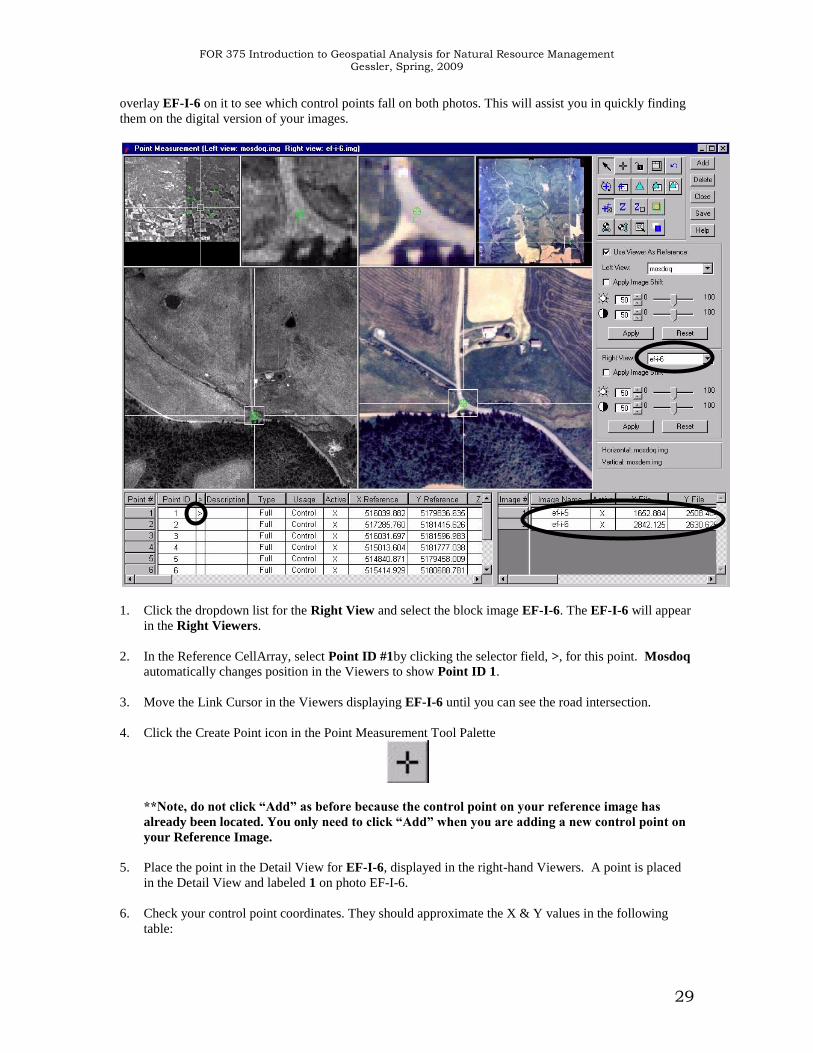
1. Click the dropdown list for the Right View and select the block image EF-I-6. The EF-I-6 will appear
in the Right Viewers.
2. In the Reference CellArray, select Point ID #1by clicking the selector field, >, for this point. Mosdoq
automatically changes position in the Viewers to show Point ID 1.
3. Move the Link Cursor in the Viewers displaying EF-I-6 until you can see the road intersection.
4. Click the Create Point icon in the Point Measurement Tool Palette
**Note, do not click “Add” as before because the control point on your reference image has
already been located. You only need to click “Add” when you are adding a new control point on
your Reference Image.
5. Place the point in the Detail View for EF-I-6, displayed in the right-hand Viewers. A point is placed
in the Detail View and labeled 1 on photo EF-I-6.
6. Check your control point coordinates. They should approximate the X & Y values in the following
table:

FOR 375 Introduction to Geospatial Analysis for Natural Resource Management Gessler, Spring, 2009
30
Image Name X File Y File
ef-i-6 2842.125 2630.625
Note: The Image CellArray now shows two rows indicating two GCP points, located on both EF-I-5
and EF-I-6, for the single GCP #1 of the reference image.
7. Continue selecting other GCPs within the Reference CellArray that correspond to both EF-I-5 and EF-
I-6. Follow the same procedures as listed in 1-5 above.
8. Once you have identified all GCPs that are located on both EF-I-5 and EF-I-6, collect additional
GCPs for the EF-I-6 image in areas that are not located on EF-I-5. For these points you will need to
click “Add” to add new control points on your left reference image. Following the previous steps on
collecting GCPs, collect a combined total of 10 GCPs for EF-I-6. Remember to mark and number
these GCPs on your EF-I-6 photo. Also be sure to distribute your points around the edges of your
photo.
Collect Ground Control Points for EF-I-7:
Next, you will collect GCPs for the next block image file (EF-I-7). You first must collect points based on
those you have already collected in EF-I-6. On your photo, locate all GCPs that you collected in EF-I-6
that can be located on EF-I-7.
1. Click the dropdown list in the Right View Tools and select the block image EF-I-7. The EF-I-7 will
appear in the Right Viewers.
2. In the Reference CellArray, select a Point ID # that is common to both EF-I-6 and EF-I-7 by clicking
the selector field, >, for this point. Mosdoq automatically changes position in the Viewers to show the
Point ID.
3. Move the Link Cursor in the Viewers displaying EF-I-7 until you can see the same location as in the
Reference Viewer.
4. Click the Create Point icon in the Point Measurement Tool Palette.
5. Click the approximate point Detail View for EF-I-7, displayed in the right three Viewers. A point is
placed in the Detail View and labeled.
6. Continue selecting and locating GCPs that correspond to both EF-I-6 and EF-I-7.
7. Once you have identified all GCPs that are located within both EF-I-6 and EF-I-7, collect additional
GCPs within the EF-I-7 image in areas that are not located with either EF-I-5 or EF-I-6. Following
the previous steps on collecting GCPs, collect a combined total of 10 GCPs for EF-I-7. Remember to
mark and number these GCPs on your EF-I-7 photo.
8. When you have completed collecting GCPs on the EF-I-7 image, click the Save button in the Point
Measurement Tool Palette.
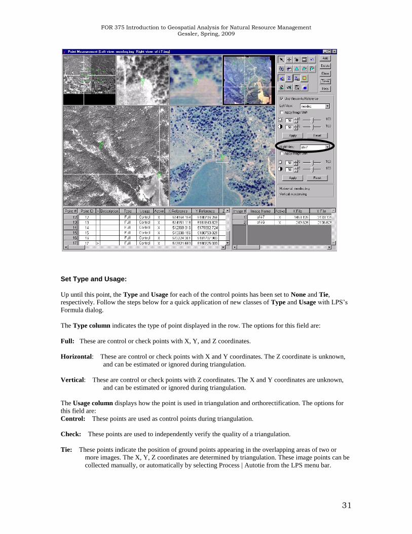
FOR 375 Introduction to Geospatial Analysis for Natural Resource Management Gessler, Spring, 2009
31
Set Type and Usage:
Up until this point, the Type and Usage for each of the control points has been set to None and Tie,
respectively. Follow the steps below for a quick application of new classes of Type and Usage with LPS’s
Formula dialog.
The Type column indicates the type of point displayed in the row. The options for this field are:
Full: These are control or check points with X, Y, and Z coordinates.
Horizontal: These are control or check points with X and Y coordinates. The Z coordinate is unknown,
and can be estimated or ignored during triangulation.
Vertical: These are control or check points with Z coordinates. The X and Y coordinates are unknown,
and can be estimated or ignored during triangulation.
The Usage column displays how the point is used in triangulation and orthorectification. The options for
this field are:
Control: These points are used as control points during triangulation.
Check: These points are used to independently verify the quality of a triangulation.
Tie: These points indicate the position of ground points appearing in the overlapping areas of two or
more images. The X, Y, Z coordinates are determined by triangulation. These image points can be
collected manually, or automatically by selecting Process | Autotie from the LPS menu bar.
FOR 375 Introduction to Geospatial Analysis for Natural Resource Management Gessler, Spring, 2009
32
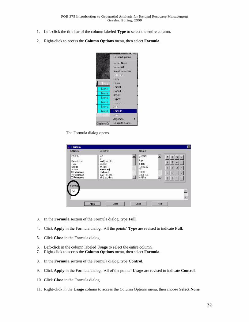
1. Left-click the title bar of the column labeled Type to select the entire column.
2. Right-click to access the Column Options menu, then select Formula.
The Formula dialog opens.
3. In the Formula section of the Formula dialog, type Full.
4. Click Apply in the Formula dialog. All the points’ Type are revised to indicate Full.
5. Click Close in the Formula dialog.
6. Left-click in the column labeled Usage to select the entire column.
7. Right-click to access the Column Options menu, then select Formula.
8. In the Formula section of the Formula dialog, type Control.
9. Click Apply in the Formula dialog. All of the points’ Usage are revised to indicate Control.
10. Click Close in the Formula dialog.
11. Right-click in the Usage column to access the Column Options menu, then choose Select None.
FOR 375 Introduction to Geospatial Analysis for Natural Resource Management Gessler, Spring, 2009
33
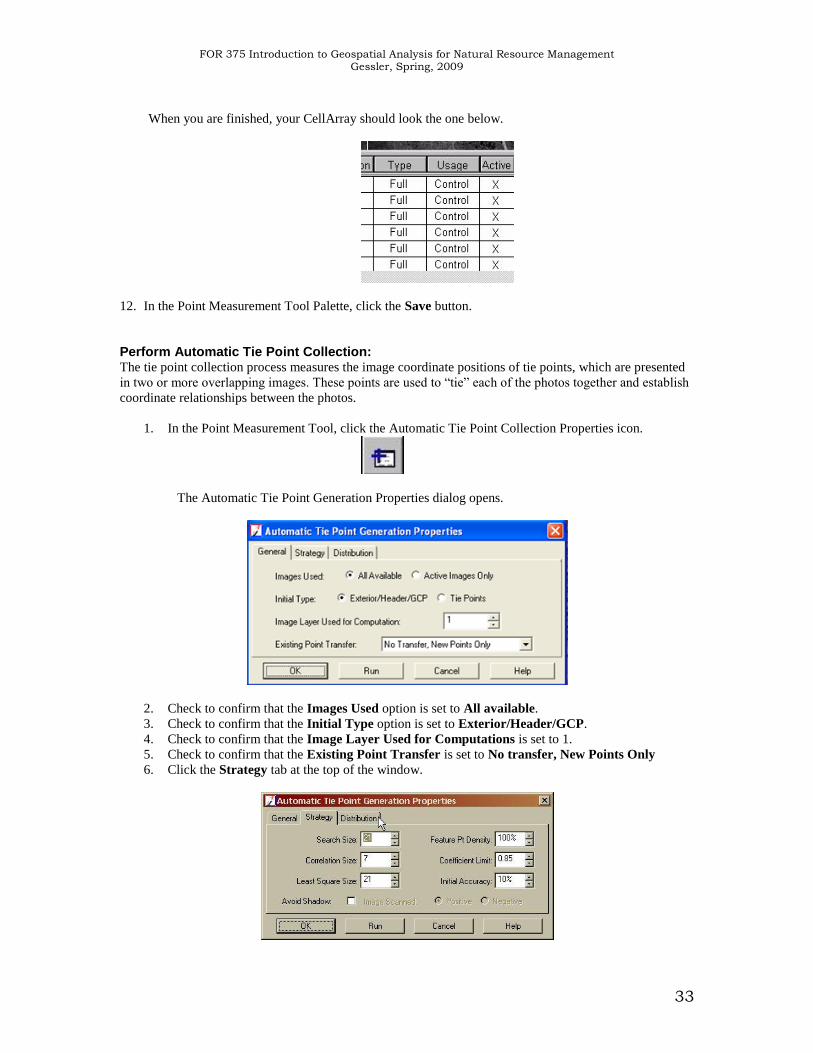
When you are finished, your CellArray should look the one below.
12. In the Point Measurement Tool Palette, click the Save button.
Perform Automatic Tie Point Collection: The tie point collection process measures the image coordinate positions of tie points, which are presented
in two or more overlapping images. These points are used to “tie” each of the photos together and establish
coordinate relationships between the photos.
1. In the Point Measurement Tool, click the Automatic Tie Point Collection Properties icon.
The Automatic Tie Point Generation Properties dialog opens.
2. Check to confirm that the Images Used option is set to All available.
3. Check to confirm that the Initial Type option is set to Exterior/Header/GCP.
4. Check to confirm that the Image Layer Used for Computations is set to 1.
5. Check to confirm that the Existing Point Transfer is set to No transfer, New Points Only
6. Click the Strategy tab at the top of the window.
FOR 375 Introduction to Geospatial Analysis for Natural Resource Management Gessler, Spring, 2009
34
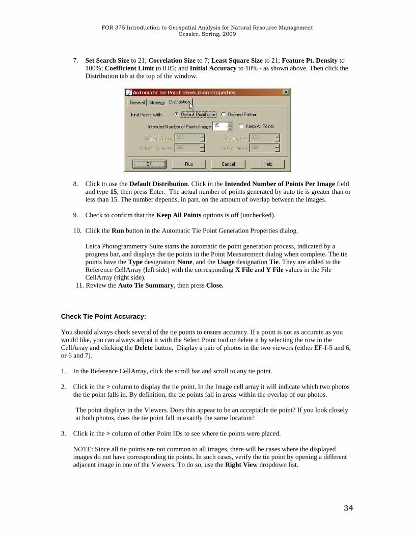
7. Set Search Size to 21; Correlation Size to 7; Least Square Size to 21; Feature Pt. Density to
100%; Coefficient Limit to 0.85; and Initial Accuracy to 10% - as shown above. Then click the
Distribution tab at the top of the window.
8. Click to use the Default Distribution. Click in the Intended Number of Points Per Image field
and type 15, then press Enter. The actual number of points generated by auto tie is greater than or
less than 15. The number depends, in part, on the amount of overlap between the images.
9. Check to confirm that the Keep All Points options is off (unchecked).
10. Click the Run button in the Automatic Tie Point Generation Properties dialog.
Leica Photogrammetry Suite starts the automatic tie point generation process, indicated by a
progress bar, and displays the tie points in the Point Measurement dialog when complete. The tie
points have the Type designation None, and the Usage designation Tie. They are added to the
Reference CellArray (left side) with the corresponding X File and Y File values in the File
CellArray (right side).
11. Review the Auto Tie Summary, then press Close.
Check Tie Point Accuracy:
You should always check several of the tie points to ensure accuracy. If a point is not as accurate as you
would like, you can always adjust it with the Select Point tool or delete it by selecting the row in the
CellArray and clicking the Delete button. Display a pair of photos in the two viewers (either EF-I-5 and 6,
or 6 and 7).
1. In the Reference CellArray, click the scroll bar and scroll to any tie point.
2. Click in the > column to display the tie point. In the Image cell array it will indicate which two photos
the tie point falls in. By definition, the tie points fall in areas within the overlap of our photos.
The point displays in the Viewers. Does this appear to be an acceptable tie point? If you look closely
at both photos, does the tie point fall in exactly the same location?
3. Click in the > column of other Point IDs to see where tie points were placed.
NOTE: Since all tie points are not common to all images, there will be cases where the displayed
images do not have corresponding tie points. In such cases, verify the tie point by opening a different
adjacent image in one of the Viewers. To do so, use the Right View dropdown list.
FOR 375 Introduction to Geospatial Analysis for Natural Resource Management Gessler, Spring, 2009
35
4. If the position of a tie point needs to be adjusted, click the Select point icon and move it in the Detail
View.
5. When you are finished, click the Save button.
6. Click the Close button to close the Point Measurement dialog. You are returned to the main
IMAGINE OrthoBASE dialog.
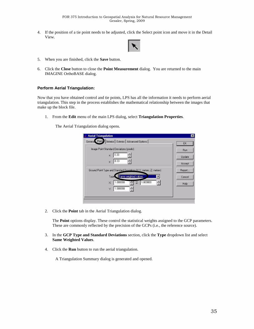
Perform Aerial Triangulation:
Now that you have obtained control and tie points, LPS has all the information it needs to perform aerial
triangulation. This step in the process establishes the mathematical relationship between the images that
make up the block file.
1. From the Edit menu of the main LPS dialog, select Triangulation Properties.
The Aerial Triangulation dialog opens.
2. Click the Point tab in the Aerial Triangulation dialog.
The Point options display. These control the statistical weights assigned to the GCP parameters.
These are commonly reflected by the precision of the GCPs (i.e., the reference source).
3. In the GCP Type and Standard Deviations section, click the Type dropdown list and select
Same Weighted Values.
4. Click the Run button to run the aerial triangulation.
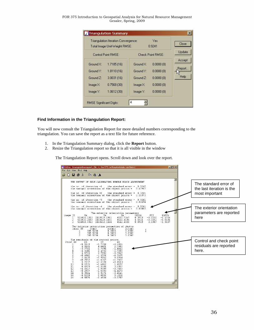
A Triangulation Summary dialog is generated and opened.
FOR 375 Introduction to Geospatial Analysis for Natural Resource Management Gessler, Spring, 2009
36
Find Information in the Triangulation Report:
You will now consult the Triangulation Report for more detailed numbers corresponding to the
triangulation. You can save the report as a text file for future reference.
1. In the Triangulation Summary dialog, click the Report button.
2. Resize the Triangulation report so that it is all visible in the window
The Triangulation Report opens. Scroll down and look over the report.
The standard error of the last iteration is the most important
The exterior orientation parameters are reported here
Control and check point residuals are reported here.
FOR 375 Introduction to Geospatial Analysis for Natural Resource Management Gessler, Spring, 2009
37
Check the Results:
1. Scroll down until you reach The Output of Self-calibrating Bundle Block Adjustment section of the
report.
2. Note the standard error of iteration number in your report. This value is the standard deviation of
unit weight, and measures the global quality of that iteration.
3. Note the exterior orientation parameters. These are the exterior orientation parameters associated
with each image in the block file. Remember we did not have this information regarding the
camera/aircraft orientation at time of acquisition. It has now been computed for us.
4. Note the residuals of the control points. The control X, Y, and Z residuals define the precision
quality in both the average residual and the geometric mean residual.
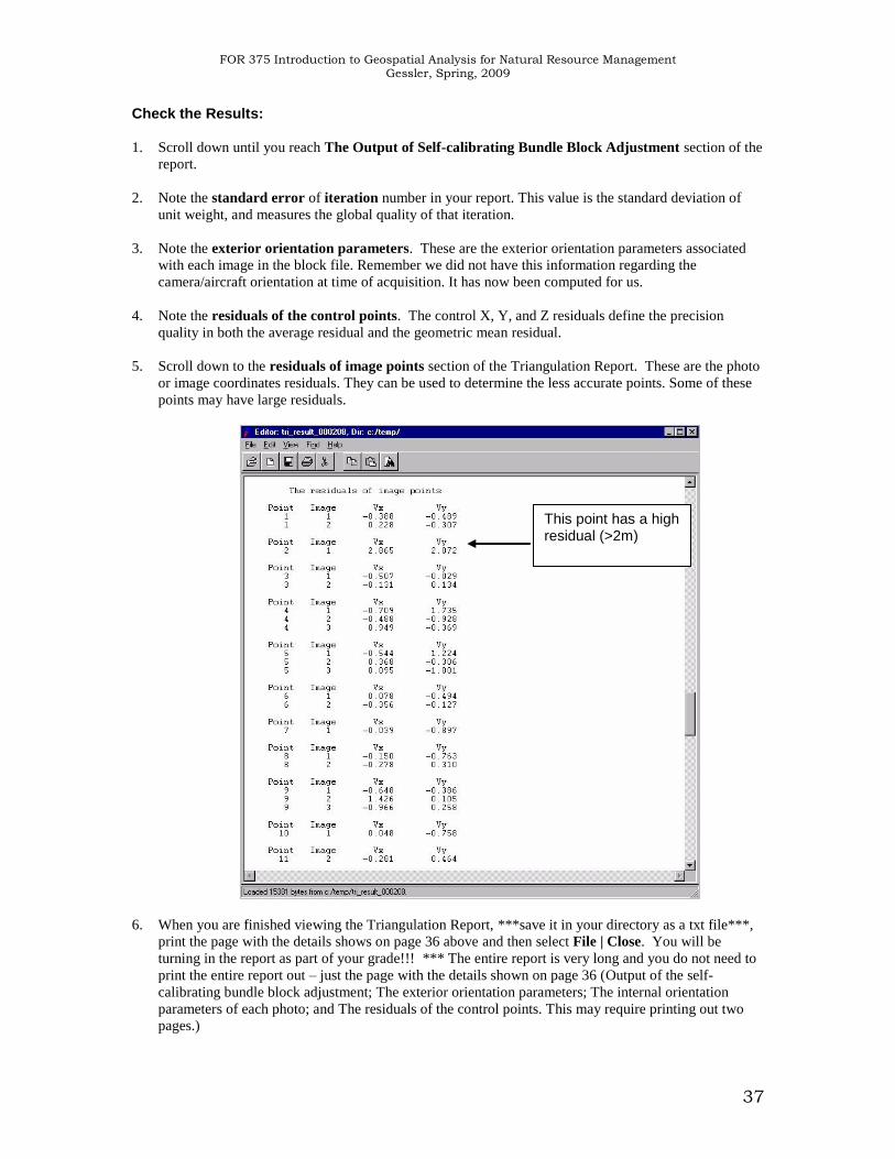
5. Scroll down to the residuals of image points section of the Triangulation Report. These are the photo
or image coordinates residuals. They can be used to determine the less accurate points. Some of these
points may have large residuals.
6. When you are finished viewing the Triangulation Report, ***save it in your directory as a txt file***,
print the page with the details shows on page 36 above and then select File | Close. You will be
turning in the report as part of your grade!!! *** The entire report is very long and you do not need to
print the entire report out – just the page with the details shown on page 36 (Output of the self-
calibrating bundle block adjustment; The exterior orientation parameters; The internal orientation
parameters of each photo; and The residuals of the control points. This may require printing out two
pages.)
This point has a high residual (>2m)
FOR 375 Introduction to Geospatial Analysis for Natural Resource Management Gessler, Spring, 2009
38
Update the Exterior Orientation:
1. In the Triangulation Summary dialog, click the Update button to update the exterior orientation
parameters. This replaces the exterior orientation parameters that were not specified during the
measurement of fiducials with the exterior orientation computed by LPS based on control and tie
points in the images making up the block file.
2. Click the Close button to close the Triangulation Summary dialog. In the Aerial Triangulation
dialog, click the Accept button to accept the triangulation parameters.
3. Click OK in the Aerial Triangulation dialog to close it. The main LPS dialog is updated to reflect
the completion of the exterior orientation step. Notice that the Ext. column is now green.
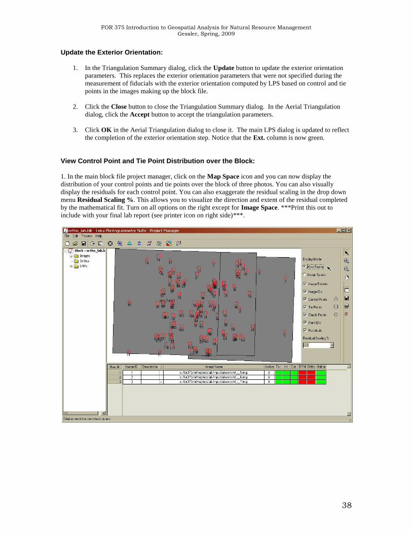
View Control Point and Tie Point Distribution over the Block:
1. In the main block file project manager, click on the Map Space icon and you can now display the
distribution of your control points and tie points over the block of three photos. You can also visually
display the residuals for each control point. You can also exaggerate the residual scaling in the drop down
menu Residual Scaling %. This allows you to visualize the direction and extent of the residual completed
by the mathematical fit. Turn on all options on the right except for Image Space. ***Print this out to
include with your final lab report (see printer icon on right side)***.
FOR 375 Introduction to Geospatial Analysis for Natural Resource Management Gessler, Spring, 2009
39
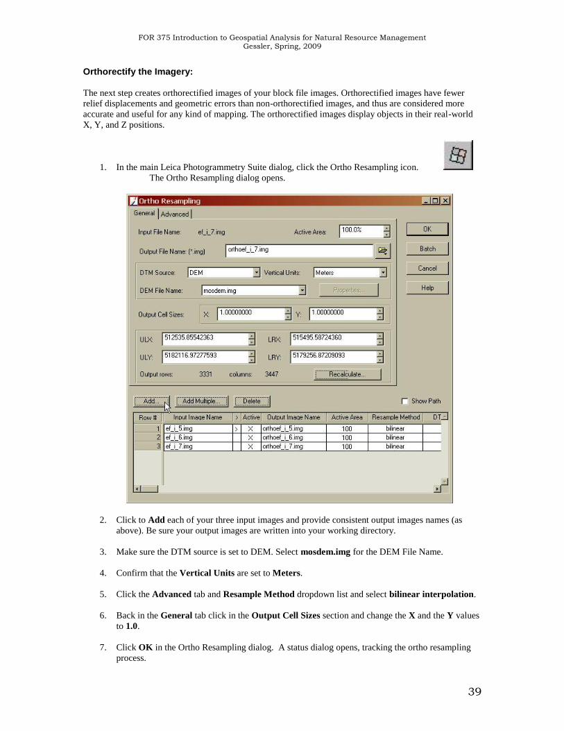
Orthorectify the Imagery:
The next step creates orthorectified images of your block file images. Orthorectified images have fewer
relief displacements and geometric errors than non-orthorectified images, and thus are considered more
accurate and useful for any kind of mapping. The orthorectified images display objects in their real-world
X, Y, and Z positions.
1. In the main Leica Photogrammetry Suite dialog, click the Ortho Resampling icon.
The Ortho Resampling dialog opens.
2. Click to Add each of your three input images and provide consistent output images names (as
above). Be sure your output images are written into your working directory.
3. Make sure the DTM source is set to DEM. Select mosdem.img for the DEM File Name.
4. Confirm that the Vertical Units are set to Meters.
5. Click the Advanced tab and Resample Method dropdown list and select bilinear interpolation.
6. Back in the General tab click in the Output Cell Sizes section and change the X and the Y values
to 1.0.
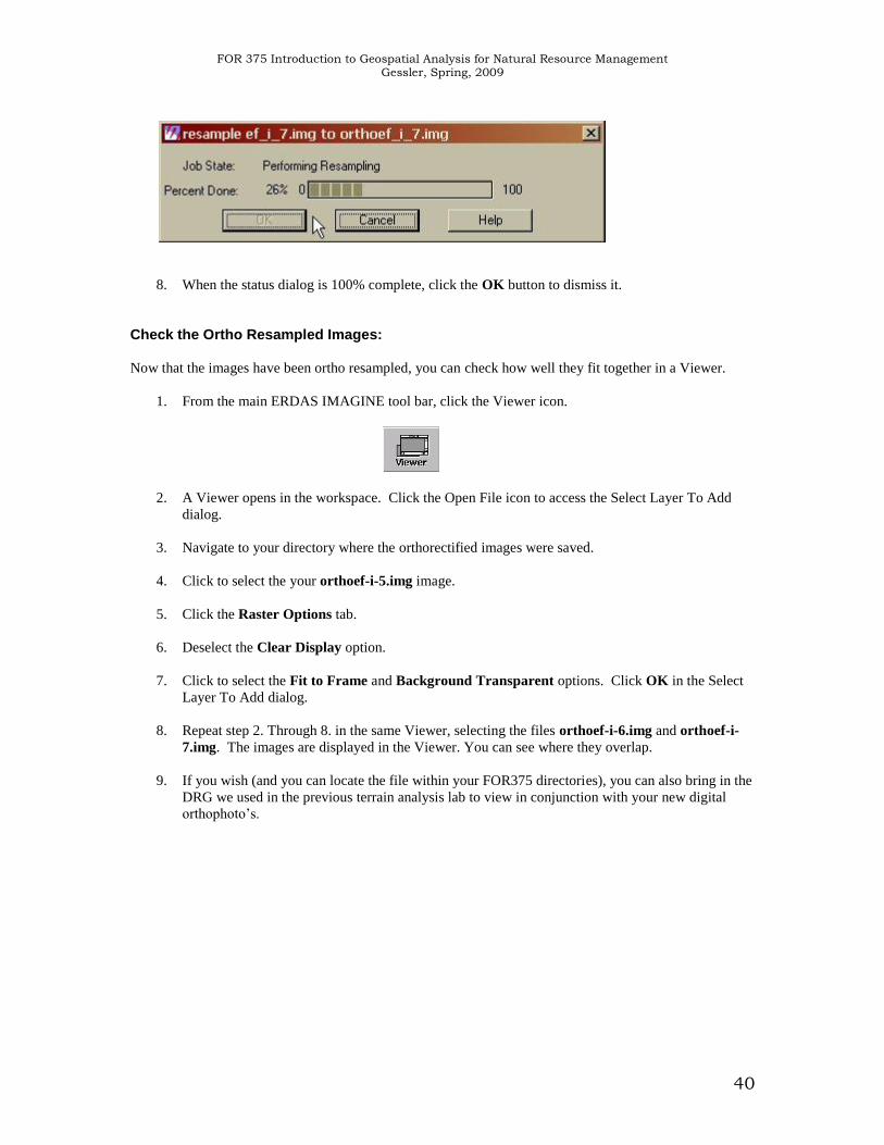
7. Click OK in the Ortho Resampling dialog. A status dialog opens, tracking the ortho resampling
process.
FOR 375 Introduction to Geospatial Analysis for Natural Resource Management Gessler, Spring, 2009
40
8. When the status dialog is 100% complete, click the OK button to dismiss it.
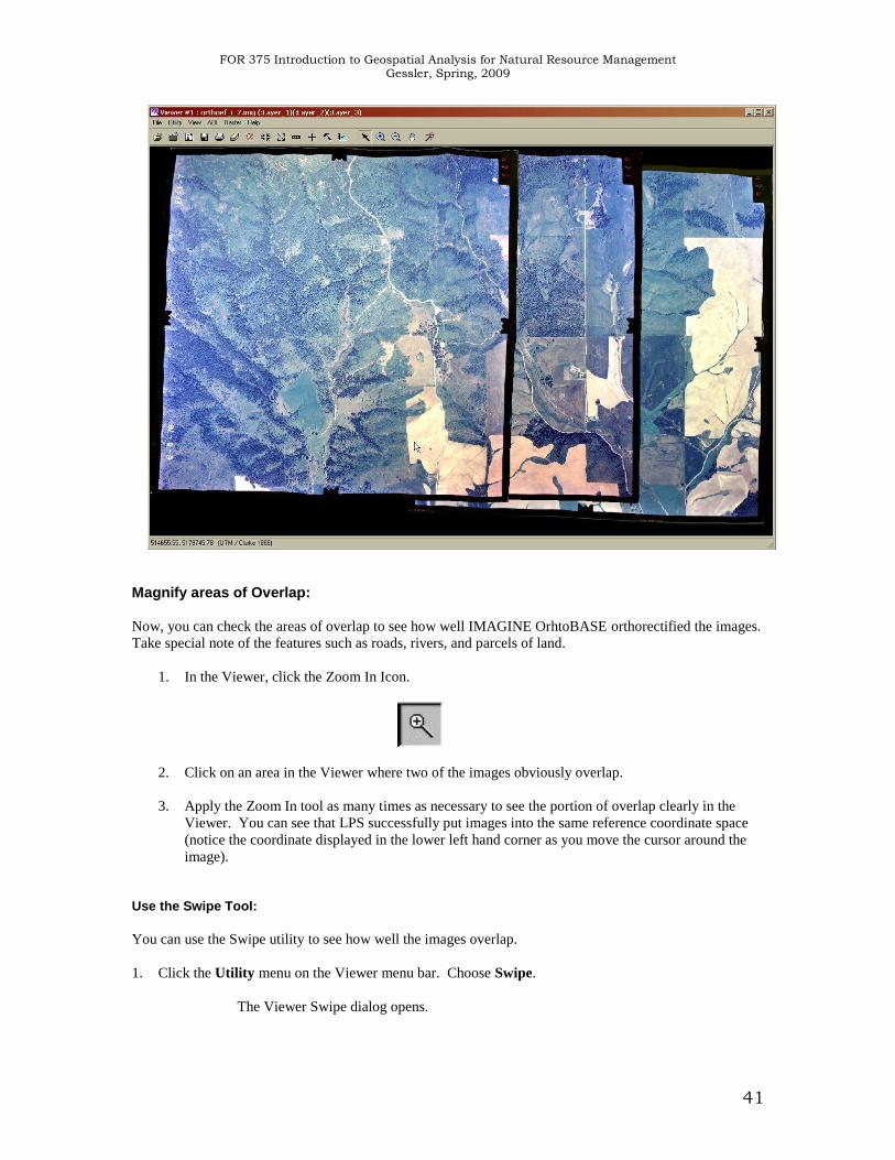
Check the Ortho Resampled Images:
Now that the images have been ortho resampled, you can check how well they fit together in a Viewer.
1. From the main ERDAS IMAGINE tool bar, click the Viewer icon.
2. A Viewer opens in the workspace. Click the Open File icon to access the Select Layer To Add
dialog.
3. Navigate to your directory where the orthorectified images were saved.
4. Click to select the your orthoef-i-5.img image.
5. Click the Raster Options tab.
6. Deselect the Clear Display option.
7. Click to select the Fit to Frame and Background Transparent options. Click OK in the Select
Layer To Add dialog.
8. Repeat step 2. Through 8. in the same Viewer, selecting the files orthoef-i-6.img and orthoef-i-
7.img. The images are displayed in the Viewer. You can see where they overlap.
9. If you wish (and you can locate the file within your FOR375 directories), you can also bring in the
DRG we used in the previous terrain analysis lab to view in conjunction with your new digital
orthophoto’s.
FOR 375 Introduction to Geospatial Analysis for Natural Resource Management Gessler, Spring, 2009
41
Magnify areas of Overlap: Now, you can check the areas of overlap to see how well IMAGINE OrhtoBASE orthorectified the images.
Take special note of the features such as roads, rivers, and parcels of land.
1. In the Viewer, click the Zoom In Icon.
2. Click on an area in the Viewer where two of the images obviously overlap.
3. Apply the Zoom In tool as many times as necessary to see the portion of overlap clearly in the
Viewer. You can see that LPS successfully put images into the same reference coordinate space
(notice the coordinate displayed in the lower left hand corner as you move the cursor around the
image).
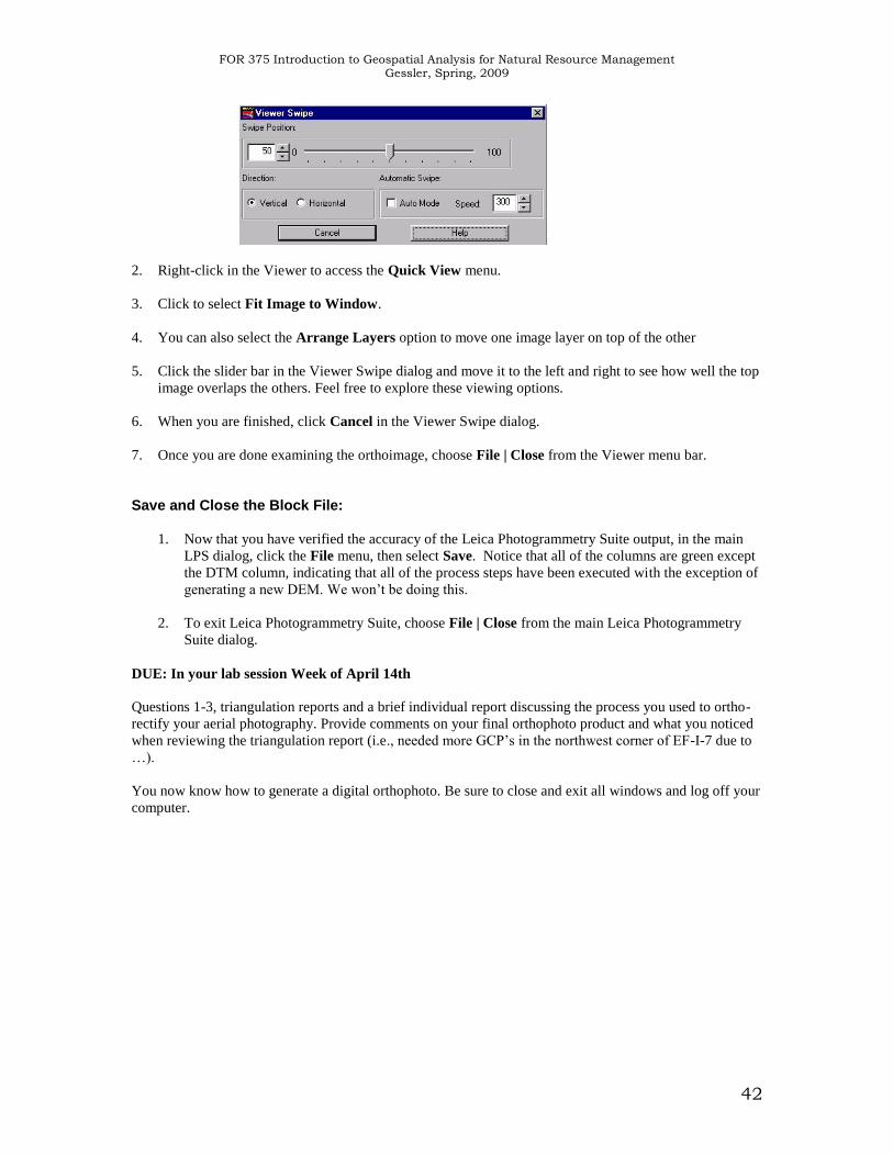
Use the Swipe Tool:
You can use the Swipe utility to see how well the images overlap.
1. Click the Utility menu on the Viewer menu bar. Choose Swipe.
The Viewer Swipe dialog opens.
FOR 375 Introduction to Geospatial Analysis for Natural Resource Management Gessler, Spring, 2009
42
2. Right-click in the Viewer to access the Quick View menu.
3. Click to select Fit Image to Window.
4. You can also select the Arrange Layers option to move one image layer on top of the other
5. Click the slider bar in the Viewer Swipe dialog and move it to the left and right to see how well the top
image overlaps the others. Feel free to explore these viewing options.
6. When you are finished, click Cancel in the Viewer Swipe dialog.
7. Once you are done examining the orthoimage, choose File | Close from the Viewer menu bar.
Save and Close the Block File:
1. Now that you have verified the accuracy of the Leica Photogrammetry Suite output, in the main
LPS dialog, click the File menu, then select Save. Notice that all of the columns are green except
the DTM column, indicating that all of the process steps have been executed with the exception of
generating a new DEM. We won’t be doing this.
2. To exit Leica Photogrammetry Suite, choose File | Close from the main Leica Photogrammetry
Suite dialog.
DUE: In your lab session Week of April 14th
Questions 1-3, triangulation reports and a brief individual report discussing the process you used to ortho-
rectify your aerial photography. Provide comments on your final orthophoto product and what you noticed
when reviewing the triangulation report (i.e., needed more GCP’s in the northwest corner of EF-I-7 due to
…).
You now know how to generate a digital orthophoto. Be sure to close and exit all windows and log off your
computer.