Journal of Educational and Behavioral Statistics

http://jebs.aera.netBehavioral Statistics

Journal of Educational and

http://jeb.sagepub.com/content/early/2012/09/27/1076998612458702The online version of this article can be found at:

DOI: 10.3102/1076998612458702

September 2012 published online 27JOURNAL OF EDUCATIONAL AND BEHAVIORAL STATISTICS

Tracy M. Sweet, Andrew C. Thomas and Brian W. JunkerSpace Models

Hierarchical Network Models for Education Research : Hierarchical Latent

Published on behalf of

American Educational Research Association

and

http://www.sagepublications.com

found at: can beJournal of Educational and Behavioral StatisticsAdditional services and information for

http://jebs.aera.net/alertsEmail Alerts:

http://jebs.aera.net/subscriptionsSubscriptions:

http://www.aera.net/reprintsReprints:

http://www.aera.net/permissionsPermissions:

What is This?

- Sep 27, 2012OnlineFirst Version of Record >>

at CARNEGIE MELLON UNIV LIBRARY on June 5, 2013http://jebs.aera.netDownloaded from

http://jebs.aera.net

http://jeb.sagepub.com/content/early/2012/09/27/1076998612458702

http://www.aera.net

http://www.sagepublications.com

http://jebs.aera.net/alerts

http://jebs.aera.net/subscriptions

http://www.aera.net/reprints

http://www.aera.net/permissions

http://jeb.sagepub.com/content/early/2012/09/27/1076998612458702.full.pdf

http://online.sagepub.com/site/sphelp/vorhelp.xhtml


Hierarchical Network Models for Education

Research: Hierarchical Latent Space Models

Tracy M. Sweet

Andrew C. Thomas

Brian W. Junker

Department of Statistics, Carnegie Mellon University

Intervention studies in school systems are sometimes aimed not at changing

curriculum or classroom technique, but rather at changing the way that

teachers, teaching coaches, and administrators in schools work with one

another—in short, changing the professional social networks of educators.

Current methods of social network analysis are ill-suited to modeling the mul-

tiple partially exchangeable networks that arise in randomized field trials and

observational studies in which multiple classrooms, schools, or districts are

involved, and to detecting the effect of an intervention on the social network

itself. To address these needs, we introduce a new modeling framework, the

Hierarchical Network Models (HNM) framework. The HNM framework can

be used to extend single-network statistical network models to multiple net-

works, using a hierarchical modeling approach. We show how to generalize the

latent space model for a single network to the HNM/multiple-network setting,

and illustrate our approach with real and simulated social network data among

education professionals.

Keywords: social network analysis, professional communities, field trials in education

research, Bayesian modeling, partial exchangeability

1 Introduction

Social network analysis (SNA) is a collection of quantitative methods for

comparing and measuring relationships among individuals in a network. Golden-

berg, Zheng, Fienberg, and Airoldi (2009) trace the development of modern

social network analysis since 1959, though social networks have been the object

of formal study as far back as Moreno (1934). Individuals and their relationships

can be represented visually as directed or undirected graphs; the nodes represent

individuals, and the edges represent asymmetric or symmetric relationships—or

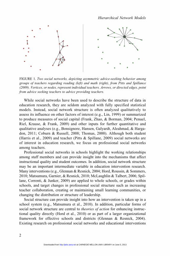
ties—between pairs of individuals. Two such networks, depicting asymmetric

advice-seeking behavior regarding two different subjects among a group of

teachers, are depicted in Figure 1.

Journal of Educational and Behavioral Statistics

2012, Vol. 00, No. 0, pp. 1–24

DOI: 10.3102/1076998612458702

# 2012 AERA. http://jebs.aera.net

1

as doi:10.3102/1076998612458702JOURNAL OF EDUCATIONAL AND BEHAVIORAL STATISTICS OnlineFirst, published on September 27, 2012



While social networks have been used to describe the structure of data in

education research, they are seldom analyzed with fully specified statistical

models. Instead, social network structure is often analyzed qualitatively to

assess its influence on other factors of interest (e.g., Lin, 1999) or summarized

to produce measures of social capital (Frank, Zhao, & Borman, 2004; Penuel,

Riel, Krause, & Frank, 2009) and other inputs for further quantitative and

qualitative analyses (e.g., Bonsignore, Hansen, Galyardt, Aleahmad, & Harga-

don, 2011; Coburn & Russell, 2008; Thomas, 2000). Although both student

(Harris et al., 2009) and teacher (Pitts & Spillane, 2009) social networks are

of interest in education research, we focus on professional social networks

among teachers.

Professional social networks in schools highlight the working relationships

among staff members and can provide insight into the mechanisms that affect

instructional quality and student outcomes. In addition, social network structure

may be an important intermediate variable in education intervention research.

Many interventions (e.g., Glennan & Resnick, 2004; Hord, Roussin, & Sommers,

2010; Matsumura, Garnier, & Resnick, 2010; McLaughlin & Talbert, 2006; Spil-

lane, Correnti, & Junker, 2009) are applied to whole schools, or grades within

schools, and target changes in professional social structure such as increasing

teacher collaboration, creating or maintaining small learning communities, or

changing the distribution or structure of leadership.

Social structure can provide insight into how an intervention is taken up in a

school system (e.g., Matsumura et al., 2010). In addition, particular forms of

social network structure are central to theories of action for enhancing instruc-

tional quality directly (Hord et al., 2010) or as part of a larger organizational

framework for effective schools and districts (Glennan & Resnick, 2004).

Existing research on professional social networks and educational interventions

FIGURE 1. Two social networks, depicting asymmetric advice-seeking behavior among

groups of teachers regarding reading (left) and math (right), from Pitts and Spillance

(2009). Vertices, or nodes, represent individual teachers. Arrows, or directed edges, point

from advice seeking teachers to advice providing teachers.

Hierarchical Network Models

2



supports these claims even though these studies tend to focus on descriptive sta-

tistics (as catalogued by Kolaczyk, 2009, chap. 4).

For example, Moolenaar, Daly, and Sleegers (2010) find an association

between teacher willingness to invest in change and the centrality of their prin-

cipal, where centrality is defined as the number of teachers seeking advice from

their school’s principal. Daly, Moolenaar, Bolivar, and Burke (2010) study the

number of connections among subgroups of teachers who taught the same grade,

finding that dense subgroups were involved with the intervention at a greater

depth than sparse subgroups. In fact, Frank, Zhao, and Borman (2004) and

Penuel, Frank, and Krause (2006) both find that access to expertise through the

network was correlated with change in teacher practice. Similarly, Frank, Penuel,

Sun, Chong, and Singleton (2010) find that teachers were more likely to employ a

particular teaching practice if they were connected to teachers who also

employed that practice. Conversely, Weinbaum, Cole, Weiss, and Supovitz

(2008) find, in an observational study of social networks among teachers in

15 schools, that schools that were involved in some type of schoolwide initiative

had more ties among teachers. Penuel et al. (2010) study two schools involved in

a schoolwide initiative at two time points, and document change in network

structure in each school, possibly associated with the initiatives.

As these examples suggest, most such studies utilize descriptive statistics of

network measures, either as quantities of direct interest or as covariates in a linear

model. For example, Daly et al. (2010) compare teachers within each grade

across schools by reporting the mean number of in-ties (i.e., the mean number

of times each teacher is identified by a peer as a connection), or mean in-

degree, for each of the five schools studied. Frank et al. (2004) and Penuel

et al. (2006) use a linear combination of the number of out-ties for each teacher

as a covariate in an ordinary least squares (OLS) regression model, pooling

teachers across schools. Similarly, Moolenaar et al. (2010) use the number of

in-ties for each principal as a predictor in a hierarchical linear model (HLM),

nesting teachers within schools. Frank et al. (2010) first use friendship network

ties to cluster teachers into subgroups and then use a linear combination of the

number of out-ties as a predictor in a three-level HLM, nesting teachers within

subgroups within schools.

Although descriptive statistics of the network can be informative, using them

alone risks missing important features of the full network. For example, if the

size of the network (e.g., number of teachers) is not constant, the number of ties

must be interpreted in terms of the size of the network. This issue is more pro-

nounced when working with multiple networks, for example in an intervention

study involving several treatment and control schools of differing sizes. Even

when the networks have approximately the same size, as in Figure 1, the topology

of ties may be quite different. For example, a tie from an advice seeker to a pop-

ular advisor may be structurally different than a tie to a more isolated teacher. It

is not at all obvious how to keep such information in the system even by

Sweet et al.

3



considering additional descriptive statistics, such as the proportion of teachers

without ties. Moreover, dependence between ties within a network will affect

comparisons of descriptive statistics between networks.

An alternative approach involves building a statistical social network model,

formalizing the likelihood of observing a particular network from the space of all

possible networks. Among statistical network models currently receiving inten-

sive interest in the literature, we consider exponential random graph models

(ERGMs), latent space models (LSMs), and mixed membership stochastic block

models (MMSBMs). These will be described in more detail in Section 2.1.

Although software exists to fit each of these network models to real data, they

have seldom been used in education research. Exceptions include two policy

studies, Penuel et al. (2010) and Weinbaum et al. (2008), who fit p2 models

(Lazega & van Duijn, 1997), a type of exponential random graph models

(ERGM), to study communication among teachers regarding an initiative. Both

studies analyze types of communication across several schools by fitting a

separate, single-network model for each school. But the models for different

schools are not linked in any way, and comparisons are based exclusively on

qualitative assessments of the parameter estimates in each model.

There is a good reason for this: Existing social network models are mostly

inadequate for the types of problems studied in education research. Comparing

different treatment conditions in an intervention study requires models that can

accommodate at least two networks, as well as parameters for treatment effects.

Moreover, education interventions generally involve several schools (i.e., profes-

sional social networks) in each condition, but again existing social network

models are largely confined to fitting one network at a time.

To address these needs, we introduce a new modeling framework, the

Hierarchical Network Models (HNM) framework. This framework allows us

to borrow strength across multiple partially exchangeable networks for parameter

estimation, as well as pools information from multiple networks to assess treat-

ment and covariate effects. Other features modeled in single network models, for

example, reciprocity and transitivity, can also be incorporated into these models

but we will not address features. Some pioneering work with multilevel struc-

tures for multiple networks has been done by Zijlstra, van Duijn, and Snijders

(2006), who introduce a multilevel p2 model; Snijders and Kenny (1999), who

extend the social relations model to multiple levels; and Templin, Ho, Anderson,

and Wasserman (2003), who propose a multilevel model for ERGMs, but our

proposed framework is more general. HNMs can accommodate any ERGM,

LSM, MMSBM, or any other single-network model in a multiple-network set-

ting, as well as essentially arbitrary network level experimental interventions.

In Section 2, we briefly review the three modeling families mentioned earlier

and introduce the general HNM framework. Although this framework is quite

general, we focus for specificity on hierarchical latent space models (HLSMs)

in Section 3. We also briefly consider similarities and differences between


4



HNMs and HLMs (Raudenbush & Bryk, 2002). In Section 4, we explore fits of

HLSMs to real and simulated professional social network data in education.

Finally, in Section 5, we indicate some future directions.

2 Modeling Framework

2.1 Single-Network Models

A single social network Y among n individuals or actors can be represented by

an n� n tie matrix

Y ¼Y11 Y12 � � � Y1n

..

. ... . .

. ...

Yn1 Yn2 � � � Ynn

264

375; ð1Þ

where Yij, i; j 2 f1; . . . ; ng, is the value of the tie or edge from actor i to actor j. In

a network graph, such as those in Figure 1, each individual i is represented by a

node, and each nonzero Yij is represented by an edge between nodes i and j. If the

relationship is symmetric, like teacher collaboration, the ties are shown as simple

line segments and Y is a symmetric matrix. If the relationship is asymmetric, like

advice seeking, the ties are drawn as arrows or directed edges, as in Figure 1, and

the matrix Y need not be symmetric.

If we only collect data on the absence or presence of a tie, then

Yij ¼1; if there is a tie from i to j

0; else

�:

If instead Yij is a measure of tie strength, such as a count value or correlation, then

Yij may be an integer or real number on the positive real line, Yij 2 ½0;1Þ. Other

possibilities also exist,1 but in this article we restrict ourselves to binary or real-

valued Yij.

ERGMs (Wasserman & Pattison, 1996) represent the probability of a social

network as a function of existing network statistics and individual and tie covari-

ates. A general ERGM may be expressed as

PðY jyÞ ¼ 1

CðyÞ expXP

p¼1

yTp spðY Þ

( ); ð2Þ

where ðs1ðY Þ, . . . , sPðY ÞÞ is a set of P sufficient statistics, typically descriptive

network statistics such as number of ties and other network structures; ðy1, . . . ,

yPÞ are the corresponding parameters to be estimated for each statistic; and CðyÞis a normalizing constant.

LSMs (Hoff, Raftery, & Handcock, 2002) assume each individual in the

network occupies a position in a latent social space, analogous to

Sweet et al.

5



multidimensional scaling or latent proximity preference models. The model repre-

sents the likelihood of a tie as a function of covariates and latent space positions,

for example, teachers who are far apart in this social space are less likely to have a

tie between them. A general LSM for Bernoulli ties may be expressed as

logit P½Yij ¼ 1� ¼ bT Xij � dðZi; ZjÞ; ð3Þ

where Xij is a vector of covariates relating to Yij, b is a set of regression coeffi-

cients to be estimated, Zi and Zj are latent location variables for individuals i and

j, and dðz1; z2Þ is a distance function; for example, dðz1; z2Þ ¼ jz1 � z2j. The Zis

are interpreted as locations of the nodes in a low-dimensional Euclidean latent

space, analogous to the latent locations in a multidimensional scaling or a latent

proximity preference model (Johnson & Junker, 2003; Polak, Heiser, De Rooij,

& Busing, 2003). These positions contribute to the model through their pairwise

distances, which are invariant to rotation and translation. The probability of a tie

increases as these locations become closer together, and may also be affected by

observable covariates Xij. Clearly, Equation 3 is one member of a class of mixed

generalized linear models (GLMs) that can be adapted to other discrete or con-

tinuous tie values Yij by changing the link function and error distribution.

Finally, MMSBMs (Airoldi, Blei, Fienberg, & Xing, 2008) allow individuals to

move between latent classes or blocks, as ties with other individuals are consid-

ered; the likelihood of a tie between two individuals is determined by their group

membership. A general MMSBM for Bernoulli tie data may be expressed as

Yij � BernoulliðSTi!jBRj iÞ

Si!j � Multinomialð1; �iÞRj i � Multinomialð1; �jÞ;

ð4Þ

where the vectors �i of multinomial probabilities and the matrix B of Bernoulli

probabilities are to be estimated. Si!j indicates which latent class or block node i

belongs to, when sending a tie to j. Similarly, Rj i indicates which latent class

(block) node j belongs to, when receiving a tie from i. Thus, the nodes exhibit

mixed block membership, potentially belonging to a different block for each tie

considered. This model generalizes the usual stochastic block model (SBM, e.g.,

Snijders & Nowicki, 1997), in which each node belongs to one and only one

block. Covariates may be added to the model by building GLM structures for the

�is or for the entries in B, for example.

2.2 Hierarchical Network Models

Turning now to our new framework for multiple-network models, we denote a

collection of K networks as Y ¼ ðY1; . . . ;YKÞ where Yk is an nk � nk tie matrix

like that of Equation 1, for the nk individuals in network k. Then, adding a

network subscript k to the tie variables in Equation 1, Yijk is the value of the tie


6



from individual i to individual j in network k. For example, in Figure 1, we have

K ¼ 2, n1 ¼ 28, and n2 ¼ 27. Once again, the tie values may be binary

(Yijk 2 f0; 1g), positive valued and unbounded (Yijk 2 ½0;1Þ), or may have some

other specification.

To build our hierarchical Bayes generalization of the single network models in

Section 2.1, we first write a likelihood, or general Level 1 model, for the ensem-

ble Y of K networks,

PðYjX;�Þ ¼YKk¼1

PðYk jXk ¼ ðX1k ; . . . ;XPkÞ;�k ¼ ðy1k ; . . . ; yQkÞÞ; ð5Þ

where PðYk jXk ;�kÞ is one of the probability models in Section 2.1 (or indeed

any other statistical model) for a single network Yk with covariates Xk , and

parameters �k .

We then specify a very general Level 2 model for �k as a hierarchical distri-

bution F with hyperparameters c and other possible covariates Wk ,

ð�1; . . . ;�KÞ � Fð�1; . . . ;�K jW1; . . . ;WK ;cÞ:The underlying distribution F may be conceptualized as a super-population dis-

tribution from which particular networks are sampled, or as a Bayesian prior distri-

bution and may be elaborated in various ways. For example, if F is specified so that

�k �iid F�ð�jcÞ; k ¼ 1; . . . ;K;

then the networks Yk are exchangeable. Speaking generatively, �ks are drawn iid

from F�, and then ties are generated randomly from the models specificed by the

�ks. Illustrations of the resulting networks are shown under the sets of ties for

each of the K networks in Figure 2.

A key innovation to our approach is that we can model a dependence across

networks by choice of Wk . Note that Wk may contain the same or different cov-

ariates across networks, providing a very general way to consider dependence

across networks. Moreover, the presence of covariates Wk , and/or additional

hierarchical distribution structure on the hyperparameters c, may lead to other

structures, so that the networks are only partially exchangeable with one another

(in contrast to the fully exchangeable structure of Figure 2).

This framework allows for a variety of dependence assumptions as well as a freer

choice of social network model. In addition, our models accommodate covariates that

may be network-, individual-, or tie-specific, or some combination. For example, Xk

might contain tie-level covariates indicating that individuals i and j in network k are

in the same (observable) group, individual-level covariates measuring teacher demo-

graphic information, and network-level covariates such as school proportion of free

and reduced-price lunch status or the type of program or curriculum implemented.

Including a network-level group indicator allows us to model quantitative

differences across groups of networks in experimental or observational data, as

Sweet et al.

7



well as treatment effects in an experimental context. Let Tk be the treatment or

group indicator for network k and let a the treatment or group effect parameter.

If there are only two treatments or groups, then Tk may be binary, and a a single

real parameter. If there are multiple treatments or groups, then Tk may be a vector

of indicators, and a the corresponding vector of effects for each treatment or group.

Then a model for estimating the treatment effect/effects a may be written as

PðYjX;�; T ; aÞ ¼YKk¼1

PðYk jXk ¼ ðX1k ; ::;XPkÞ; Tk ;�k ¼ ðy1k ; ::; yQkÞ; aÞ

ð�1; . . . ;�KÞ � Fð�1; . . . ;�K jcÞa � gðajgÞðwith additional hierarchical structure; as appropriateÞ:

ð6Þ

This provides a general, partially exchangeable modeling framework for model-

ing multiple networks and estimating treatment effects.

3 HLSMs/Specializations of the HNM Framework

The hierarchical structure specified in Section 2.2 is extremely general, and

many different types of network models, including those reviewed in Section 2.1,

can be used to specify a particular HNM. Here, we show how the HLSM can be

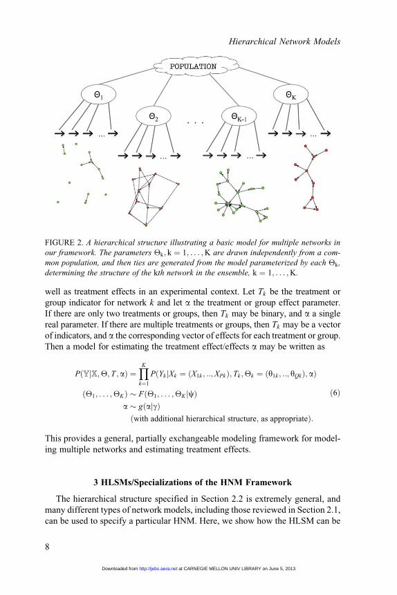
FIGURE 2. A hierarchical structure illustrating a basic model for multiple networks in

our framework. The parameters �k; k ¼ 1; . . . ;K are drawn independently from a com-

mon population, and then ties are generated from the model parameterized by each �k,

determining the structure of the kth network in the ensemble, k ¼ 1; . . . ;K.


8



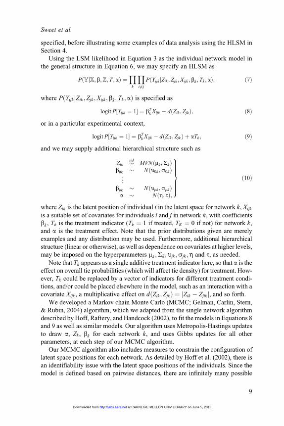
specified, before illustrating some examples of data analysis using the HLSM in

Section 4.

Using the LSM likelihood in Equation 3 as the individual network model in

the general structure in Equation 6, we may specify an HLSM as

PðYjX; b;Z; T ; aÞ ¼Y

k

Yi6¼j

PðYijk jZik ; Zjk ;Xijk ; bk ; Tk ; aÞ; ð7Þ

where PðYijk jZik ; Zjk ;Xijk ; bk ; Tk ; aÞ is specified as

logit P½Yijk ¼ 1� ¼ bTk Xijk � dðZik ; ZjkÞ; ð8Þ

or in a particular experimental context,

logit P½Yijk ¼ 1� ¼ bTk Xijk � dðZik ; ZjkÞ þ aTk ; ð9Þ

and we may supply additional hierarchical structure such as

Zik �iid MVNðmk ;SkÞb0k � Nðυ0k ;s0kÞ

..

.

bpk � Nðυpk ;spkÞa � Nðη; tÞ;

9>>>>>=>>>>>;

ð10Þ

where Zik is the latent position of individual i in the latent space for network k, Xijk

is a suitable set of covariates for individuals i and j in network k, with coefficients

bk , Tk is the treatment indicator (Tk ¼ 1 if treated, TK ¼ 0 if not) for network k,

and a is the treatment effect. Note that the prior distributions given are merely

examples and any distribution may be used. Furthermore, additional hierarchical

structure (linear or otherwise), as well as dependence on covariates at higher levels,

may be imposed on the hyperparameters mk ;Sk ;υjk;sjk;η and t, as needed.

Note that Tk appears as a single additive treatment indicator here, so that a is the

effect on overall tie probabilities (which will affect tie density) for treatment. How-

ever, Tk could be replaced by a vector of indicators for different treatment condi-

tions, and/or could be placed elsewhere in the model, such as an interaction with a

covariate Xijk , a multiplicative effect on dðZik; ZjkÞ ¼ jZik � Zjik j, and so forth.

We developed a Markov chain Monte Carlo (MCMC; Gelman, Carlin, Stern,

& Rubin, 2004) algorithm, which we adapted from the single network algorithm

described by Hoff, Raftery, and Handcock (2002), to fit the models in Equations 8

and 9 as well as similar models. Our algorithm uses Metropolis-Hastings updates

to draw a, Zk , bk for each network k, and uses Gibbs updates for all other

parameters, at each step of our MCMC algorithm.

Our MCMC algorithm also includes measures to constrain the configuration of

latent space positions for each network. As detailed by Hoff et al. (2002), there is

an identifiability issue with the latent space positions of the individuals. Since the

model is defined based on pairwise distances, there are infinitely many possible

Sweet et al.

9



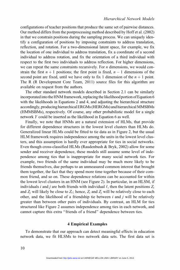
configurations of teacher positions that produce the same set of pairwise distances.

Our method differs from the postprocessing method described by Hoff et al. (2002)

in that we constrain positions during the sampling process. We can uniquely iden-

tify a configuration of positions by imposing constraints to address translation,

reflection, and rotation. For a two-dimensional latent space, for example, we fix

the location of one individual to address translation, fix a coordinate of a second

individual to address rotation, and fix the orientation of a third individual with

respect to the first two individuals to address reflection. For higher dimensions,

we can repeat the same constraints recursively. For n dimensions, we would con-

strain the first nþ 1 positions; the first point is fixed, n� 1 dimensions of the

second point are fixed, until we have only to fix 1 dimension of the nþ 1 point.

The R (R Development Core Team, 2011) source files for this algorithm are

available on request from the authors.

The other standard network models described in Section 2.1 can be similarly

incorporated into theHNM framework, replacing the likelihoodportion of Equation 6

with the likelihoods in Equations 2 and 4, and adjusting the hierarchical structure

accordingly, producinghierarchical ERGMs (HERGMs) andhierarchical MMSBMs

(HMMSBMs), respectively. Of course, any other probabilistic model for a single

network Y could be inserted as the likelihood in Equation 6 as well.

Finally, we note that HNMs are a natural extension of HLMs, that provide

for different dependence structures in the lowest level clusters than HLMs do.

Generalized linear HLMs could be fitted to tie data as in Figure 2, but the usual

HLM framework requires independence among the units in the lowest level clus-

ters, and this assumption is hardly ever appropriate for ties in social networks.

Even though cross-classified HLMs (Raudenbush & Bryk, 2002) allow for some

sender and receiver dependence, these models still assume some level of inde-

pendence among ties that is inappropriate for many social network ties. For

example, two friends of the same individual may be much more likely to be

friends themselves, due perhaps to an unmeasured common interest that brought

them together, the fact that they spend more time together because of their com-

mon friend, and so on. These dependence relations can be accounted for within

the lowest level clusters in an HNM (see Figure 2). In particular, in an HLSM, if

individuals i and j are both friends with individual ‘, then the latent positions Zi

and Zj will likely be close to Z‘; hence, Zi and Zj will be relatively close to each

other, and the likelihood of a friendship tie between i and j will be relatively

greater than between other pairs of individuals. By contrast, an HLM for ties

structured like Figure 2 assumes independence among ties in each network, and

cannot capture this extra ‘‘friends of a friend’’ dependence between ties.

4 Empirical Examples

To demonstrate that our approach can detect meaningful effects in education

network data, we fit HLSMs to two network data sets. The first data set is


10



composed of teachers whose ties indicate the seeking of professional advice, col-

lected by Pitts and Spillane (2009); our application shows that the model can

detect the effect of tie-level covariates. The second data set is simulated data,

which we use to explore the utility and operating characteristics for detecting

network-level treatment effects.

4.1 Covariate Effects in an Observational Study

Pitts and Spillance (2009) surveyed teachers and principals in 15 elementary

and middle schools from a large, urban school district to validate a school staff

survey instrument. These schools include both private and public schools ranging

from pre-kindergarten to eighth grade and vary in the number of staff members.

School staff were asked to list to whom they seek advice and include the fre-

quency and value they place on the advisor. Additional demographic data and

belief measures were also collected.

Networks consist of teachers who responded to the network portion of the sur-

vey and other teachers identified as tie recipients. Schools varied in network size,

the smallest network of 12 teachers and the largest of 76 teachers. Table 1 lists

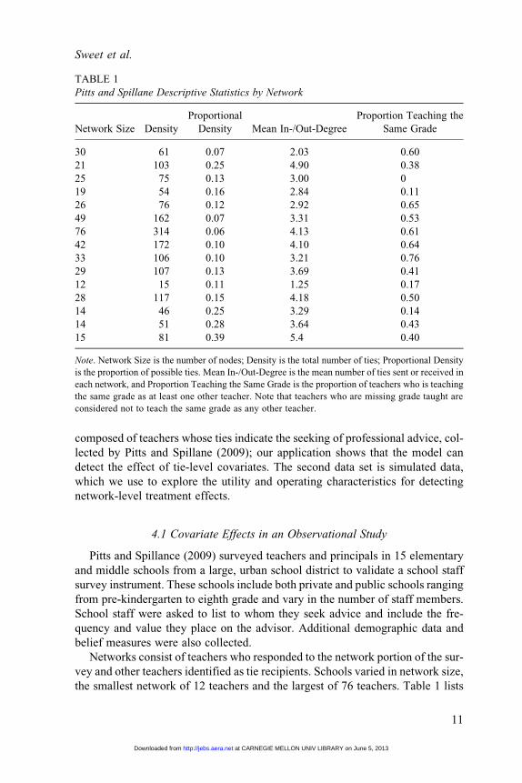
TABLE 1

Pitts and Spillane Descriptive Statistics by Network

Network Size Density

Proportional

Density Mean In-/Out-Degree

Proportion Teaching the

Same Grade

30 61 0.07 2.03 0.60

21 103 0.25 4.90 0.38

25 75 0.13 3.00 0

19 54 0.16 2.84 0.11

26 76 0.12 2.92 0.65

49 162 0.07 3.31 0.53

76 314 0.06 4.13 0.61

42 172 0.10 4.10 0.64

33 106 0.10 3.21 0.76

29 107 0.13 3.69 0.41

12 15 0.11 1.25 0.17

28 117 0.15 4.18 0.50

14 46 0.25 3.29 0.14

14 51 0.28 3.64 0.43

15 81 0.39 5.4 0.40

Note. Network Size is the number of nodes; Density is the total number of ties; Proportional Density

is the proportion of possible ties. Mean In-/Out-Degree is the mean number of ties sent or received in

each network, and Proportion Teaching the Same Grade is the proportion of teachers who is teaching

the same grade as at least one other teacher. Note that teachers who are missing grade taught are

considered not to teach the same grade as any other teacher.

Sweet et al.

11



network size and other descriptive network statistics for each school. Smaller

schools tend to have a higher number of ties relative to network size whereas

schools tend to have similar numbers of ties per teacher, regardless of size. In

addition to network statistics, we include in Table 1 one edge-level variable, the

proportion of teachers who taught the same grade as at least 1 other teacher.

Although schools include subsets of grades pre-k through 8, this proportion

varies widely by school. This is due to missing data since teachers who did not

report their grade assignment cannot be matched. There are four schools for

which missing data is so extensive that less than 20% of the teachers are teaching

the same grade as another teacher.

For these data, we fit a simple HLSM with a single tie-specific covariate;

X1ijk ¼ 1 if teacher i and j in school k teach the same grade and 0 otherwise. For

simplicity, teachers who did not report their grade taught are assumed not to

teach the same grade as any other teacher.

We specify the model as

logit P½Yijk ¼ 1� ¼ b0k þ b1kX1ijk � jZik � Zjk j;

Zik � MVN0

0

� �;

10 0

0 10

� �� ; i ¼ 1; . . . ; nk ;

b0k � Nðm0;s20Þ; k ¼ 1; . . . ;K;

b1k � Nðm1;s21Þ; k ¼ 1; . . . ;K;

m0 � Nð0; 1Þ;m1 � Nð0; 1Þ;s2

0 � Inv� Gammað100; 150Þ;s2

1 � Inv� Gammað100; 150Þ;

ð11Þ

where K ¼ 15, the total number of schools. We model the latent space positions

for teachers in each school as two-dimensional. Furthermore, we impose an addi-

tional hierarchical structure by estimating the hyperparameters m0, m1, s20, s2

1.

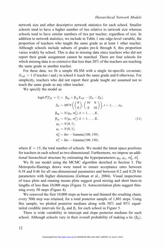
We fit our model using the MCMC algorithm sketched in Section 3. The

Metropolis-Hastings draws were tuned to ensure acceptance rates between

0.38 and 0.46 for all one-dimensional parameters and between 0.2 and 0.28 for

parameters with higher dimensions (Gelman et al., 2004). Visual inspections

of trace plots and running means plots suggest good mixing and short burn-in

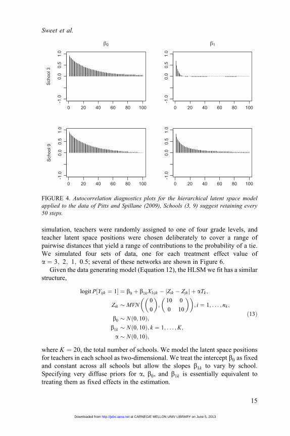
lengths of less than 10,000 steps (Figure 3). Autocorrelation plots suggest thin-

ning every 50 steps (Figure 4).

We removed the first 10,000 steps as burn-in and thinned the resulting chain;

every 50th step was retained, for a total posterior sample of 1,801 steps. Using

this sample, we plotted posterior medians along with 50% and 95% equal-

tailed credible intervals for b0 and b1 for each school in Figure 5.

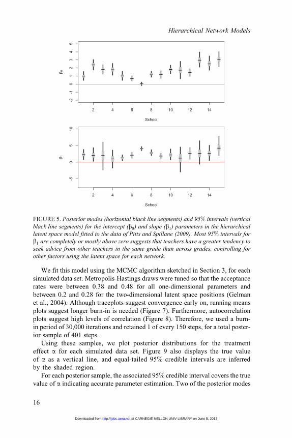
There is wide variability in intercept and slope posterior medians for each

school. Although schools vary in their overall probability of making a tie ðb0Þ,


12



there seems to be a positive effect of teaching the same grade (b1). We model b0

and b1 from normal distributions, see Section 4.1. Posterior means are (1.50,

1.47) and (1.85, 4.34) for ðm0;s20Þ and ðm1;s

21Þ, respectively. Moreover, the

95% credible interval for m1 is (0.77, 2.93), so the global effect of teaching the

same grade is positive.

There are several possible explanations for the variability in b0 across schools.

Some variability is expected, as schools vary in the social structure of their teach-

ers, but there are other possible explanations as well. There are several schools,

Schools 6 through 10 and 12, which have much larger networks than the other

schools. The intercept for these schools would naturally be a bit lower, since the

overall probability of a tie between two teachers would decrease, as the number

of individuals within a school increases. In fact, the schools with large positive

intercepts are the schools smallest in size, Schools 11, 13, 14, and 15 with 15

or fewer teachers. These schools also happen to be parochial schools.

Regarding b1, the effect of teaching the same grade, we expect the size of the

school to be correlated with the coefficient estimates since schools with many

teachers teaching the same grade are less likely to have mutual ties than schools

with only a few teachers teaching the same grade. Rather, what we find is the size

of the school, coupled with the amount of grade assignment data available, drives

the variability in the b1 estimates. Large schools tend to have more data available

and the four largest schools, Schools 6 through 9, generally have small variability

in their estimates for b1. Schools that are either small or have little information

regarding teacher grade assignment have large variability; Schools 3, 4, 11, and

13 have relatively little information, and Schools 11, 13, 14, and 15 have the

fewest numbers of teachers. For comparison, we also fit separate single-

network LSMs for each of the 15 schools. The posterior spreads for b1 are

unacceptably large for several of the schools. Schools 3, 11, 13, and 15 have

b1 posterior variances of 104, 54, 41, and 32, respectively.

4.2 Treatment Effects in a Controlled Experiment

We do not yet have social network data involving a controlled, network-level

intervention. However, studies like Spillane, Correnti, and Junker (2009) offer

the promise of such data in the near future. In the meantime, we have simulated

several social network data sets, to explore the utility and operating characteris-

tics of our models for detecting treatment effects.

Each simulated data set consists of 20 schools, with 10 teachers in each

school. We generated undirected, binary network ties from the model

logitP½Yijk ¼ 1� ¼ 2þ 4X1ijk � jZik � Zjk j þ aTk ; ð12Þ

where half of the schools are assigned to be treatment schools (Tk ¼ 1) and the

other half are control schools. We included only one other covariate, the tie-level

binary indicator that teacher i and teacher j teach the same grade. In the

Sweet et al.

13



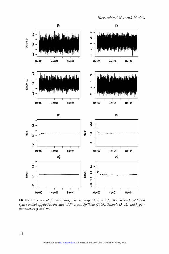
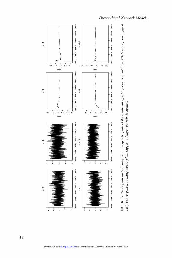
FIGURE 3. Trace plots and running means diagnostics plots for the hierarchical latent

space model applied to the data of Pitts and Spillane (2009), Schools (5, 12) and hyper-

parameters m and s2.


14



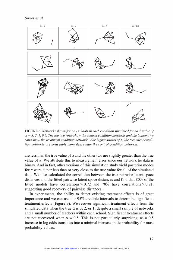
simulation, teachers were randomly assigned to one of four grade levels, and

teacher latent space positions were chosen deliberately to cover a range of

pairwise distances that yield a range of contributions to the probability of a tie.

We simulated four sets of data, one for each treatment effect value of

a ¼ 3; 2; 1; 0:5; several of these networks are shown in Figure 6.

Given the data generating model (Equation 12), the HLSM we fit has a similar

structure,

logit P½Yijk ¼ 1� ¼ b0 þ b1kX1ijk � jZik � Zjk j þ aTk ;

Zik � MVN0

0

� �;

10 0

0 10

� �� ; i ¼ 1; . . . ; nk ;

b0 � Nð0; 10Þ;b1k � Nð0; 10Þ; k ¼ 1; . . . ;K;

a � Nð0; 10Þ;

ð13Þ

where K ¼ 20, the total number of schools. We model the latent space positions

for teachers in each school as two-dimensional. We treat the intercept b0 as fixed

and constant across all schools but allow the slopes b1k to vary by school.

Specifying very diffuse priors for a, b0, and b1k is essentially equivalent to

treating them as fixed effects in the estimation.

0 20 40 60 80 100

-1.0

0.0

0.5

1.0

0S

choo

l 3

0 20 40 60 80 100

-1.0

0.0

0.5

1.0

1

0 20 40 60 80 100

-1.0

0.0

0.5

1.0

Sch

ool 9

0 20 40 60 80 100

-1.0

0.0

0.5

1.0

FIGURE 4. Autocorrelation diagnostics plots for the hierarchical latent space model

applied to the data of Pitts and Spillane (2009), Schools (3, 9) suggest retaining every

50 steps.

Sweet et al.

15



We fit this model using the MCMC algorithm sketched in Section 3, for each

simulated data set. Metropolis-Hastings draws were tuned so that the acceptance

rates were between 0.38 and 0.48 for all one-dimensional parameters and

between 0.2 and 0.28 for the two-dimensional latent space positions (Gelman

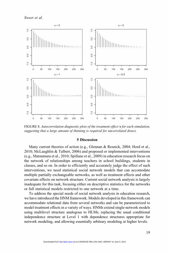
et al., 2004). Although traceplots suggest convergence early on, running means

plots suggest longer burn-in is needed (Figure 7). Furthermore, autocorrelation

plots suggest high levels of correlation (Figure 8). Therefore, we used a burn-

in period of 30,000 iterations and retained 1 of every 150 steps, for a total poster-

ior sample of 401 steps.

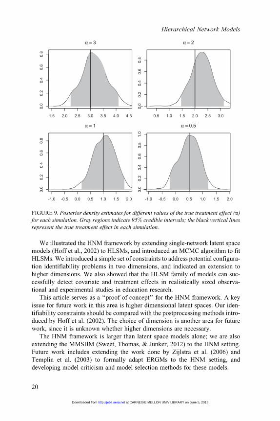
Using these samples, we plot posterior distributions for the treatment

effect a for each simulated data set. Figure 9 also displays the true value

of a as a vertical line, and equal-tailed 95% credible intervals are inferred

by the shaded region.

For each posterior sample, the associated 95% credible interval covers the true

value of a indicating accurate parameter estimation. Two of the posterior modes

2 4 6 8 10 12 14

-2-1

01

23

45

School

0

2 4 6 8 10 12 14

-50

510

School

1

FIGURE 5. Posterior modes (horizontal black line segments) and 95% intervals (vertical

black line segments) for the intercept (b0) and slope (b1) parameters in the hierarchical

latent space model fitted to the data of Pitts and Spillane (2009). Most 95% intervals for

b1 are completely or mostly above zero suggests that teachers have a greater tendency to

seek advice from other teachers in the same grade than across grades, controlling for

other factors using the latent space for each network.


16



are less than the true value of a and the other two are slightly greater than the true

value of a. We attribute this to measurement error since our network tie data is

binary. And in fact, other versions of this simulation study yield posterior modes

for a were either less than or very close to the true value for all of the simulated

data. We also calculated the correlation between the true pairwise latent space

distances and the fitted pairwise latent space distances and find that 80% of the

fitted models have correlations > 0:72 and 70% have correlations > 0:81,

suggesting good recovery of pairwise distances.

In experiments, the ability to detect existing treatment effects is of great

importance and we can use our 95% credible intervals to determine significant

treatment effects (Figure 9). We recover significant treatment effects from the

simulated data when the true a is 3, 2, or 1, despite a small sample of networks

and a small number of teachers within each school. Significant treatment effects

are not recovered when a ¼ 0:5. This is not particularly surprising, as a 0.5

increase in log odds translates into a minimal increase in tie probability for most

probability values.

= 3 = 2 = 1 = 0.5

FIGURE 6. Networks shown for two schools in each condition simulated for each value of

a ¼ 3, 2, 1, 0.5. The top two rows show the control condition networks and the bottom two

rows show the treatment condition networks. For higher values of a, the treatment condi-

tion networks are noticeably more dense than the control condition networks.

Sweet et al.

17



FIG

UR

E7.T

race

plo

tsand

runnin

gm

eans

dia

gnost

icplo

tsof

the

trea

tmen

tef

fecta

for

each

sim

ula

tion.

Whil

etr

ace

plo

tssu

gges

t

earl

yco

nve

rgen

ce,

runnin

gm

eans

plo

tssu

gges

ta

longer

burn

-in

isnee

ded

.


18



5 Discussion

Many current theories of action (e.g., Glennan & Resnick, 2004; Hord et al.,

2010; McLaughlin & Talbert, 2006) and proposed or implemented interventions

(e.g., Matsumura et al., 2010; Spillane et al., 2009) in education research focus on

the network of relationships among teachers in school buildings, students in

classes, and so on. In order to efficiently and accurately judge the effect of such

interventions, we need statistical social network models that can accomodate

multiple partially exchangeable networks, as well as treatment effects and other

covariate effects on network structure. Current social network analysis is largely

inadequate for this task, focusing either on descriptive statistics for the networks

or full statistical models restricted to one network at a time.

To address the special needs of social network analysis in education research,

we have introduced the HNM framework. Models developed in this framework can

accommodate relational data from several networks and can be parameterized to

model treatment effects in a variety of ways. HNMs extend single-network models

using multilevel structure analogous to HLMs, replacing the usual conditional

independence structure at Level 1 with dependence structures appropriate for

network modeling, and allowing essentially arbitrary modeling at higher levels.

0 50 100 150 200 250 300

-1.0

-0.5

0.0

0.5

1.0

= 3

0 50 100 150 200 250 300

-1.0

-0.5

0.0

0.5

1.0

= 2

0 50 100 150 200 250 300

-1.0

-0.5

0.0

0.5

1.0

= 1

0 50 100 150 200 250 300

-1.0

-0.5

0.0

0.5

1.0

= 0.5

FIGURE 8. Autocorrelation diagnostic plots of the treatment effect a for each simulation,

suggesting that a large amount of thinning is required for uncorrelated draws.

Sweet et al.

19



We illustrated the HNM framework by extending single-network latent space

models (Hoff et al., 2002) to HLSMs, and introduced an MCMC algorithm to fit

HLSMs. We introduced a simple set of constraints to address potential configura-

tion identifiability problems in two dimensions, and indicated an extension to

higher dimensions. We also showed that the HLSM family of models can suc-

cessfully detect covariate and treatment effects in realistically sized observa-

tional and experimental studies in education research.

This article serves as a ‘‘proof of concept’’ for the HNM framework. A key

issue for future work in this area is higher dimensional latent spaces. Our iden-

tifiability constraints should be compared with the postprocessing methods intro-

duced by Hoff et al. (2002). The choice of dimension is another area for future

work, since it is unknown whether higher dimensions are necessary.

The HNM framework is larger than latent space models alone; we are also

extending the MMSBM (Sweet, Thomas, & Junker, 2012) to the HNM setting.

Future work includes extending the work done by Zijlstra et al. (2006) and

Templin et al. (2003) to formally adapt ERGMs to the HNM setting, and

developing model criticism and model selection methods for these models.

1.5 2.0 2.5 3.0 3.5 4.0 4.5

0.0

0.2

0.4

0.6

0.8

α = 3 α = 2

α = 1 α = 0.5

0.5 1.0 1.5 2.0 2.5 3.0

0.0

0.2

0.4

0.6

0.8

-1.0 -0.5 0.0 0.5 1.0 1.5 2.0

0.0

0.2

0.4

0.6

0.8

-1.0 -0.5 0.0 0.5 1.0 1.5 2.0

0.0

0.2

0.4

0.6

0.8

1.0

FIGURE 9. Posterior density estimates for different values of the true treatment effect (a)

for each simulation. Gray regions indicate 95% credible intervals; the black vertical lines

represent the true treatment effect in each simulation.


20



The HNM framework is well suited to estimating treatment and covariate

effects in multiple-network experiments. Often, however, changes in the social

network are intermediate variables for an intervention whose intended ‘‘final’’

outcome is student achievement or a similar variable (e.g., McLaughlin &

Talbert, 2006). Since the HNM is itself a multilevel model, it can be emebedded

as the intermediate level of a multilevel model for the outcome of interest—in

this way, social network structure need not be ignored in studies of other educa-

tional outcomes of interest.

Declaration of Conflicting Interests

The authors declared no potential conflicts of interest with respect to the research, author-

ship, and/or publication of this article.

Funding

The authors disclosed receipt of the following financial support for the research, author-

ship and/or publication of this article: Program for Interdisciplinary Education Research,

supported by the Institute for Education Sciences, Department of Education, Grant

R305B040063. The opinions expressed are those of the authors and do not necessarily

represent views of the Institute or the U.S. Department of Education.

Note

1. For example, if we measure not only the number of contacts between teacher i

and teacher j but also the average length of time of a contact, then each Yij

would be an ordered pair of these values.

References

Airoldi, E., Blei, D., Fienberg, S., & Xing, E. (2008). Mixed membership stochastic block-

models. The Journal of Machine Learning Research, 9, 1981–2014.

Bonsignore, E., Hansen, D., Galyardt, A., Aleahmad, T., & Hargadon, S. (2011). The

power of social networking for professional development. In T. Gray & H. Silver-

Pacuilla (Eds.), Breakthrough teaching and learning: How educational and assistive

technologies are driving innovation (pp. 25–52). New York, NY: Springer.

Coburn, C., & Russell, J. (2008). District policy and teachers’ social networks. Educa-

tional Evaluation and Policy Analysis, 30, 203–235.

Daly, A., Moolenaar, N., Bolivar, J., & Burke, P. (2010). Relationships in reform: The role

of teachers’ social networks. Journal of Educational Administration, 48, 359–391.

Fienberg, S., Meyer, M., & Wasserman, S. (1985). Statistical analysis of multiple socio-

metric relations. Journal of the American Statistical Association, 80, 51–67.

Frank, K. A., Penuel, W. R., Sun, M., Chong, M. K., & Singleton, C. (2013). The

organization as a filter of institutional diffusion. Teachers College Record, 115(1).

Frank, K. A., Zhao, Y., & Borman, K. (2004). Social capital and the diffusion of innova-

tions within organizations: The case of computer technology in schools. Sociology of

Education, 77, 148–171.

Gelman, A., Carlin, J., Stern, H., & Rubin, D. (2004). Bayesian data analysis. Boca Raton,

FL: CRC press.

Sweet et al.

21



Glennan, T. K., & Resnick, L. B. (2004). Expanding the reach of education reforms

perspectives from leaders in the scale-up of educational interventions. In T. K. Glennan,

S. J. Bodill, J. R. Galegher, & K. A. Kerr (Eds.), School districts as learning organizations:

A strategy for scaling education reform (Chap. 14, pp. 517–563). Santa Monica, CA:

RAND Corporation.

Goldenberg, A., Zheng, A., Fienberg, S., & Airoldi, E. (2009). A survey of statistical net-

work models. Foundations and Trends in Machine Learning, 2, 129–133.

Harris, K., Halpern, C., Whitsel, E., Hussey, J., Tabor, J., Entzel, P., & Udry, J. (2009).

The national longitudinal study of adolescent health: Research design. Retrieved from

http://www.cpc.unc.edu/projects/addhealth/design

Hoff, P. D., Raftery, A. E., & Handcock, M. S. (2002). Latent space approaches to social

network analysis. Journal of the American Statistical Association, 97, 1090–1098.

Hord, S., Roussin, J., & Sommers, W. (2010). Guiding professional learning communities:

Inspiration, challenge, surprise and meaning. Thousand Oaks, CA: Corwin/Sage.

Johnson, M., & Junker, B. (2003). Using data augmentation and Markov chain Monte

Carlo for the estimation of unfolding response models. Journal of Educational and

Behavioral Statistics, 28, 195.

Kolaczyk, E. (2009). Statistical analysis of network data: Methods and models. New

York, NY: Springer-Verlag.

Lazega, E., & van Duijn, M. (1997). Position in formal structure, personal characteristics

and choices of advisors in a law firm: A logistic regression model for dyadic network

data. Social Networks, 19, 375–397.

Lin, N. (1999). Building a network theory of social capital. Connections, 22, 28–51.

Matsumura, L., Garnier, H., & Resnick, L. (2010). Implementing literacy coaching: The

role of school social resources. Educational Evaluation and Policy Analysis, 32,

249–272.

McLaughlin, M., & Talbert, J. (2006). Building school-based teacher learning commu-

nities: Professional strategies to improve student achievement (Vol. 45). New York,

NY: Teachers College Press.

Moreno, J. (1934). Who shall survive?: A new approach to the problem of human inter-

relations. Washington, DC: Nervous and Mental Disease.

Moolenaar, N., Daly, A., & Sleegers, P. (2010). Occupying the principal position: Exam-

ining relationships between transformational leadership, social network position, and

schools’ innovative climate. Educational Administration Quarterly, 46, 623.

Penuel, W., Riel, M., Joshi, A., Pearlman, L., Kim, C., & Frank, K. (2010). The alignment

of the informal and formal organizational supports for reform: Implications for

improving teaching in schools. Educational Administration Quarterly, 46, 57–95.

Penuel, W., Riel, M., Krause, A., & Frank, K. (2009). Analyzing teachers’ professional

interactions in a school as social capital: A social network approach. The Teachers Col-

lege Record, 111, 124–163.

Penuel, W. R., Frank, K. A., & Krause, A. (2006). The distribution of resources and exper-

tise and the implementation of schoolwide reform initiatives. In Proceedings of the 7th

international conference on Learning sciences, ICLS ’06 (pp. 522–528). Indiana

University, Bloomington, IN: International Society of the Learning Sciences.

Pitts, V., & Spillane, J. (2009). Using social network methods to study school leadership.

International Journal of Research & Method in Education, 32, 185–207.


22



Polak, M., Heiser, W., De Rooij, M., & Busing, F. (July 2003). A comparison of corre-

spondence analysis, multidimensional unfolding and the generalized graded unfolding

model for single-peaked data. Paper presented at the 13th International Meeting of the

Psychometric Society Chia Laguna (Cagliari), Italy.

R Development Core Team. (2011). R: A language for data analysis and graphics.

Vienna, Austria: R Foundation for Statistical Computing.

Raudenbush, S., & Bryk, A. (2002). Hierarchical linear models: Applications and data

analysis methods (Vol. 1). Thousand Oaks, CA: Sage.

Snijders, T., & Kenny, D. (1999). The social relations model for family data: A multilevel

approach. Personal Relationships, 6, 471–486.

Snijders, T., & Nowicki, K. (1997). Estimation and prediction for stochastic blockmodels

for graphs with latent block structure. Journal of Classification, 14, 75–100.

Spillane, J., Correnti, R., & Junker, B. (2009). Learning leadership: Kernel routines for

instructional improvement. (IES Grant Proposal.) Chicago, IL: Author.

Sweet, T., Thomas, A. C., & Junker, B. (2012). Handbook on mixed membership models,

chapter Hierarchical Mixed Membership Stochastic Blockmodels for Multiple Net-

works and Experimental Interventions. New York, NY: Chapman & Hall/CRC. invited

chapter.

Templin, J., Ho, M.-H., Anderson, C., & Wasserman, S. (2003). Mixed effects p* model

for multiple social networks. In Proceedings of the American Statistical Association:

Bayesian Statistical Sciences Section, (pp. 4198-4024). Alexandria, VA: American

Statistical Association.

Thomas, S. (2000). Ties that bind: A social network approach to understanding student

integration and persistence. The Journal of Higher Education, 71, 591–615.

Wasserman, S., & Pattison, P. (1996). Logit models and logistic regressions for social

networks: I. An introduction to Markov graphs and p*. Psychometrika, 61,

401–425. doi:10.1007/BF02294547

Weinbaum, E., Cole, R., Weiss, M., & Supovitz, J. (2008). Going with the flow: Commu-

nication and reform in high schools. In J. Supovitz & E. Weinbaum (Eds.), The imple-

mentation gap: Understanding reform in high schools (pp. 68–102). New York, NY:

Teachers College Press.

Zijlstra, B., van Duijn, M., & Snijders, T. (2006). The multilevel p 2 model. Methodology:

European Journal of Research Methods for the Behavioral and Social Sciences, 2,

42–47.

Authors

TRACY M. SWEET is a post-doctoral fellow in the Statistics department at Carnegie

Mellon University, Pittsburgh, PA 15213; [email protected]. Her research

interests include education statistics, and in particular, research methodology for

large-scale experiments and social network analysis of professional communities.

ANDREW C. THOMAS is a visiting assistant professor in the Statistics department at

Carnegie Mellon University, Pittsburgh, PA 15213; [email protected]. In addi-

tion to his research on social network analysis, his research interests include statistics

in the social and political sciences, sports statistics, and biostatistics.

Sweet et al.

23



BRIAN W. JUNKER is a professor in the Statistics department at Carnegie Mellon

University, Pittsburgh, PA 15213; [email protected]. His research interests include

nonparametric and Bayesian item response theory and unfolding models, hierarchical

models for multiple ratings of extended-response test items, psychometric cognitive

diagnosis models and predictive modeling of online tutoring systems, multiple-

recapture census systems, mixed effects models and sampling weights in large-scale

surveys, causal modeling, Markov chain Monte Carlo and other computing and estima-

tion methods, errors in variables, factor analysis and structural equation models in

econometrics and psychiatric statistics, statistical analysis of large randomized field

trials in education, rating protocols for teacher quality, educational data mining, social

network analysis, and grade of membership or latent dirichlet allocation models.

Manuscript received December 8, 2011

Revision received March 22, 2012

Accepted June 7, 2012


24



Documents

Journal of Educational and Behavioral Statistics