Joseph Bafumi,a Robert S. Erikson,b and Christopher Wlezienc

Balancing, Generic Polls and Midterm Congressional Elections* by

Joseph Bafumi,a Robert S. Erikson,b and Christopher Wlezienc

November 2009

a Department of Government, Dartmouth College, Hanover, New Hampshire 03755;

E-mail:[email protected].

b Department of Political Science, Columbia University, New York, NY 10027;

E-mail:[email protected].

c Department of Political Science, Temple University, Philadelphia PA 19122-6089;

E-mail: [email protected].

Abstract One mystery of US politics is why the president’s party regularly loses congressional

seats at midterm. Although presidential coattails and their withdrawal provide a partial

explanation, coattails cannot account for the fact that the presidential party typically

performs worse than normal at midterm. This paper addresses the midterm vote separate

from the presidential year vote, with evidence from generic congressional polls

conducted during midterm election years. Polls early in the midterm year project a

normal vote result in November. But as the campaign progresses, vote preferences

almost always move toward the out party. This shift is not a negative referendum on the

president, as midterms do not show a pattern of declining presidential popularity or

increasing salience of presidential performance. The shift accords with “balance” theory,

where the midterm campaign motivates some to vote against the party of the president in

order to achieve policy moderation.

mailto:[email protected]



One running mystery about American politics is that the winning presidential party

almost always loses congressional seats at the next midterm election. For a run of 15

straight midterm elections, 1938-1994, the presidential party suffered seat losses at

midterm. In 1998, Clinton’s Democrats gained seats but did actually suffer a slight

decline in its share of the national vote. Bush’s Republicans triumphantly won both seats

and vote share in 2002, but of course not in 2006.

At one time the prevailing explanation for midterm loss was Angus Campbell’s

(1966) “surge-and- decline” theory. Surge-and-decline dictates the winning presidential

party’s congressional support surges in response to “short-term partisan forces” in the

“high-stimulus” presidential year. These waxing forces (or presidential “coattails”) then

wane in the following midterm election as the outcome returns to the “normal” (largely

party-line) vote with the president no longer on the ballot and the related “low-stimulus”

status of the midterm campaign.1

It is true, of course, that congressional parties perform better in presidential years

when the party’s presidential candidate does well. This is the coattail phenomenon.

However the prediction of a persistent normal vote at midterm is clearly wrong. More

importantly, the presidential party’s disadvantage at midterm typically outweighs its

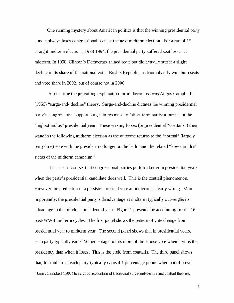
advantage in the previous presidential year. Figure 1 presents the accounting for the 16

post-WWII midterm cycles. The first panel shows the pattern of vote change from

presidential year to midterm year. The second panel shows that in presidential years,

each party typically earns 2.6 percentage points more of the House vote when it wins the

presidency than when it loses. This is the yield from coattails. The third panel shows

that, for midterms, each party typically earns 4.1 percentage points when out of power 1 James Campbell (1997) has a good accounting of traditional surge-and-decline and coattail theories.

1

than when it holds the presidency. (Both regularities pass the test of statistical

significance.) To do well in midterm House elections, it is best to lose the presidency.

Surge-and-decline theories do not fully account for why this is true.

—Figure 1 about here—

“Referendum theory” is often cited as a reason for the presidential party’s poor

midterm showing. Presidents decline in popularity from their initial honeymoon period,

and the degree of popularity can matter at midterm (Tufte, 1975; James Campbell, 1997;

Jacobson, 2004.).2 But referendum theory has one weak link if it is to explain the

midterm slump. As detailed below, presidents’ approval levels are not particularly low at

midterm compared to other non-honeymoon periods. With majorities typically

“approving” the president’s performance at midterm, it is difficult to claim that the

presidential party’s typical poor showing in midterm elections is due to voter

disillusionment with how the president is handling the job.

This leads to still a third way of accounting for midterm loss, so-called “balance”

theory. In the formulation of Alesina and Rosenthal (1990, 1994; see also Fiorina 2003),

the electorate boosts its support for the out party at midterm from a desire for balance in

terms of ideology or policy. Policy is seen as the result of the averaged party

composition of Congress and the presidency. While both parties sit in Congress, the

presidency is not divisible by party. Thus, net policy must be right of the median voter

during Republican administrations and to the left during Democratic administrations. By

putting their collective thumbs on the scale in favor of the out party at midterm, voters

2 James Campbell (1997) offers a revised surge-and-decline theory to account for change in terms of the traditional presidential year surge but with a midterm vote that is not necessarily the “low stimulus” result predicted by Angus Campbell’s original version.

2

move policy back toward the center. Sentiments toward balancing emerge and grow as

campaigns focus voters on their vote decisions.

“Balancing” theory has its own issues. Most obviously, the theory lost some

luster when it failed to predict the gaining party in the 1998 and 2002 midterm elections.

The theory must reckon with the corollary that voters might sometimes balance in

advance—in presidential years when landslide victories are universally anticipated

(Scheve and Toms, 1999). Anticipatory balancing could minimize midterm loss by

offsetting coattail effects. .

Some see ideological balancing as beyond the capability of the electorate. This

criticism may have bite when applied to “thick” balance theories, such as Mebane’s

(2000) complex model of the midterm vote as an N-person game involving voter

coordination. A “thin” version requires only that voters are motivated by a perceived

policy difference between the parties, plus a knowledge of the president’s party.3

The present paper addresses that portion of midterm loss generated during the

midterm year. We make use of a unique data set—the results of national polls predicting

the congressional vote in midterm years using the “generic ballot” question, which asks

respondents for which party (not candidate) they intend to vote. We have measured

generic ballot responses for six separate time periods in the campaign calendar over all 16

3 Variations of these theories deserve mention. Jacobson and Kernell’s (1983) “strategic politicians” theory posits that congressional election outcomes are in large part generated by politicians anticipating electoral trends and capitalizing on them. For instance, if the midterm year is seen as a good year for the out party, the out party can draw strong challengers. In the extreme, the politicians’ beliefs about the political climate generate a self-fulfilling prophesy. Strategic politicians theory is best seen as a complement to existing theories—as a reminder that electoral trends driven by referendum or balance processes can accelerate when the politicians believe them to be true. Kernell (1977) also introduces a “negative voting” model. He posits that out-party supporters are more motivated to vote. This sort of asymmetrical motivation could complement either referendum theory or balance theory. By either scenario, abstentions by presidential supporters would produce a result similar to that from voters shifting their votes toward the out party. A question would be why there would be this asymmetric motivation to vote at midterm but not on other electoral occasions.

3

midterm election years, 1946-2006. Our central question is whether generic ballot

respondents increasingly take the party of the president into account over the course of

midterm campaigns. Decisively, we find that they do. We then address whether the

reason for increasing motivation to vote for the “out” party at midterm year is due to

growing dissatisfaction with the president’s performance. We find that it is not. As

citizens focus more on their vote decision in the run-up to the election, they increasingly

balance against the president’s party but not in a way that is traceable to their perceptions

of presidential performance.

Balancing Theory and Midterm Electorates

The theoretical argument for balancing in midterm elections is presented by

Alesina and Rosenthal (1994).4 The conditions for the balancing argument to hold are

that some voters are motivated to move policy closer to their desired policy position and

that these voters hold beliefs about the relevant policy positions that separate the parties.

Given the usual choice between a liberal Democrat and a conservative Republican, the

president will have policy choices to the left (if Democrat) or right (if Republican) than

most voters. Congress, a blend of 535 individually elected representatives will on

average be closer to national public opinion than will the president. Thus, conditional on

knowing the presidential party, the electorate can push policy toward the center by voting

for the opposition party.5

4 Note that Alesina and Rosenthal’s balance theory is about voting for one office based on the national verdict in the other. It is not about split-ticket voting, as if voters choose from a menu of candidates for various offices based on ideological balance. 5 Ample research shows that presidents’ policy behavior provides voters motivation for balancing, as the party of the president is a powerful predictor of policy (Erikson, MacKuen and Stimson, 2002; Wlezien, 2004; Poole and Rosenthal, 2007).

4

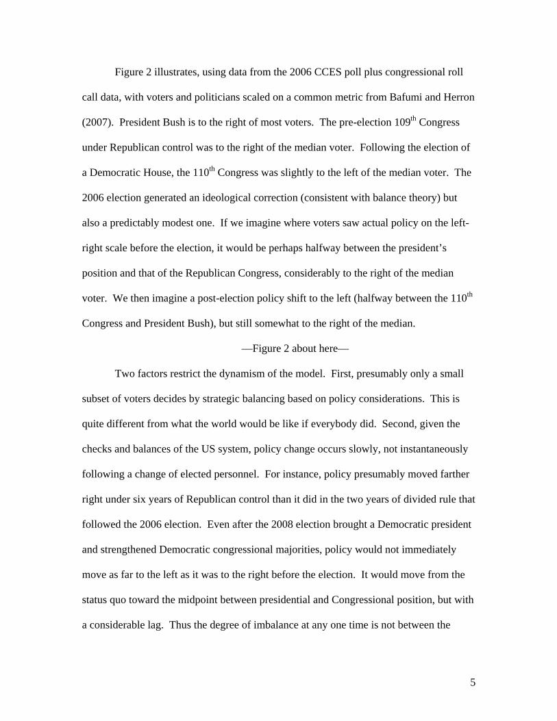
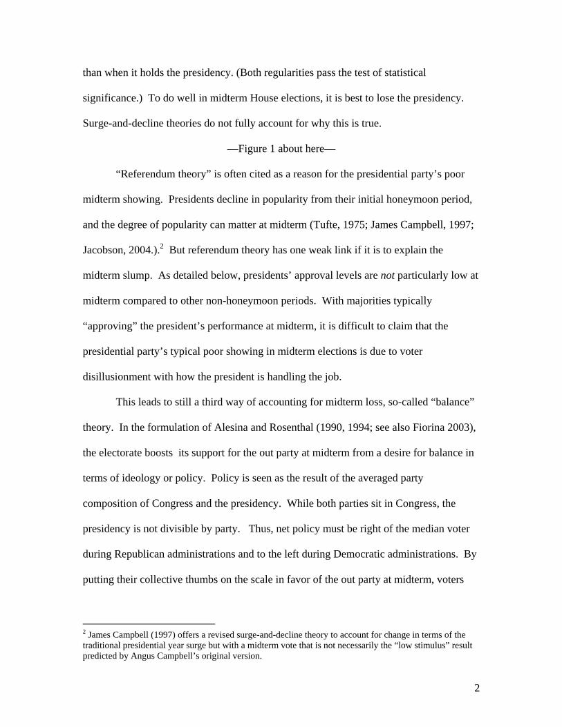
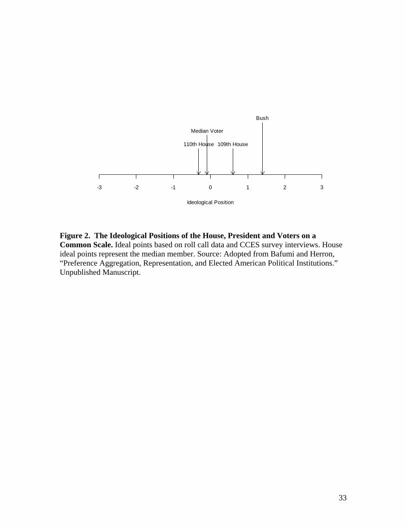
Figure 2 illustrates, using data from the 2006 CCES poll plus congressional roll

call data, with voters and politicians scaled on a common metric from Bafumi and Herron

(2007). President Bush is to the right of most voters. The pre-election 109th Congress

under Republican control was to the right of the median voter. Following the election of

a Democratic House, the 110th Congress was slightly to the left of the median voter. The

2006 election generated an ideological correction (consistent with balance theory) but

also a predictably modest one. If we imagine where voters saw actual policy on the left-

right scale before the election, it would be perhaps halfway between the president’s

position and that of the Republican Congress, considerably to the right of the median

voter. We then imagine a post-election policy shift to the left (halfway between the 110th

Congress and President Bush), but still somewhat to the right of the median.

—Figure 2 about here—

Two factors restrict the dynamism of the model. First, presumably only a small

subset of voters decides by strategic balancing based on policy considerations. This is

quite different from what the world would be like if everybody did. Second, given the

checks and balances of the US system, policy change occurs slowly, not instantaneously

following a change of elected personnel. For instance, policy presumably moved farther

right under six years of Republican control than it did in the two years of divided rule that

followed the 2006 election. Even after the 2008 election brought a Democratic president

and strengthened Democratic congressional majorities, policy would not immediately

move as far to the left as it was to the right before the election. It would move from the

status quo toward the midpoint between presidential and Congressional position, but with

a considerable lag. Thus the degree of imbalance at any one time is not between the

5

median voter and the congressional-presidential midpoint, but between the median voter

and the slower moving net policy, averaged across issues.6

An implication of these restrictions on the dynamism of the model is that

balancing behavior can reflect not only the current party balance at midterm but also

party balance from the past. Thus, for instance, the 2010 midterm electorate will balance

not only Obama’s liberalism but also the conservative policies inherited from the Bush

years. If there is also a Democratic president and Congress in place for the 2014

midterm, policy would reflect six years of Democratic dominance and policy shifting

further left. The balancing imperative would be a stronger Republican tilt at the 2014

midterm. This would be a manifestation of the “six year itch” (Abramowitz, et al. 1986),

the tendency of a party to lose more seats after six years in office than after only two.

Generic Polls of the Congressional Vote

Going back to 1946, pollsters (initially Gallup alone) have monitored the “generic

vote” during midterm campaigns. Generic trial-heat polls ask survey respondents which

party they plan to vote for (or who they want to win) in the upcoming congressional

election.7 We have gathered the record of 831 generic congressional polls in midterm

elections years beginning in 1946, from Gallup and other survey organizations, using the

Roper Center and pollingreport.com as sources. We measure the generic vote at several

intervals leading up to the midterm election date. The earliest feasible reading is for early

in the midterm year—241 to 300 days before the election, centering on February of the

6 For a discussion of why national policy responds slowly to public opinion, see Erikson et al., 2002. 7 There is considerable variation in question wording. Some organizations ask “If the election were being held today”. Other organizations use “Looking ahead to the congressional elections in November” or “Thinking about the next election for US Congress.” Given what we know about wording effects on presidential trial-heats (Lau, 1994), there is reason to think that the exact wording matters little, though there may be circumstances where they are consequential (see, e.g., McDermott and Frankovic, 2003).

6

midterm year. We also measure the generic vote during later intervals—181 to 240 days,

121 to 180 days, 61-120 days, 31-60 days, and 1-30 days before the election. Based on

the modal month for each interval, we describe the interval midpoints as February, April,

June, August, September, and October. For each interval in each of 16 midterm years we

pool the available poll readings as described in the online appendix.8

We measure both the actual vote and the verdicts in the generic congressional

polls as percentages of the two-party vote. To aid assessment of possible (partisan) poll

bias, we measure the vote and the survey-based generic vote as a deviation from the equal

division, 50% Democratic and 50% Republican. Pollsters variously report the generic

vote as among “likely voters,” “registered voters,” or “adults.” For the analysis, we

adjust the observed poll results to project our best estimates of what the result would be if

the poll were a “likely voter” poll. Details are available in the online appendix.

The answer to the question “how accurate are the generic polls?” must be nuanced

(Erikson and Sigelman, 1995; Moore and Saad, 1997). Generic polls perform poorly as

point estimates; the leading party in the polls typically ends up with a smaller lead on

Election Day. However, regression equations accounting for the vote in terms of the

generic vote do predict well, as they properly discount the exaggerated sizes of the

generic poll leads. When properly interpreted, the generic polls are far better augers of

congressional elections than their sometimes ragged reputation would have us believe.

We also employ monthly readings of party identification (or “macropartisanship”)

and of presidential approval. Macropartisanship is a useful measure of underlying

partisan sentiment. Similar to our generic vote measure, we measure party identification

8 See www.dartmouth.edu/~jbafumi for the online appendix.

7

as the percent Democratic among Democratic and Republican identifiers, relative to the

50-50 baseline.9 Presidential approval is measured in the conventional way, as the

percent who say they “approve” of the current president’s performance.10

Given that “monthly” data for generic polls, party identification, and presidential

approval are often drawn from the same surveys, there must be considerable overlap in

the respondents comprising the three aggregate measures. This is an advantage, not a

handicap. Overlapping respondents provides leverage; relationships among different

survey-based aggregate variables are more accurate if they are measured for the same

rather than different samples of respondents.

Ideological Balancing and the Midterm Campaign

It is widely agreed that the function of political campaigns is to bring the issues

of the campaign to the voters. In midterm election years, the presidential opposition

party tries to prime voters that they should elect more of its members in order to restore

partisan balance in Washington. In this section we demonstrate that this strategy almost

universally works to change congressional vote preferences over the midterm year.

The presidential party and generic ballot trial heats

We begin with the mapping of the generic congressional vote in February of the

midterm year, the earliest milepost for which we can get readings for all 16 midterm

years of our analysis. By this time point of the campaign, any coattail effects from the

previous presidential election should have dissipated. From surge and decline theory, we

9 Interestingly, unlike with the generic vote, there is no effect on party identification of being in or out of power at midterm. The mean October macropartisanship is exactly 58.3% Democratic in both the seven midterms with a Democratic president and the nine midterms with a Republican president 10 Both party identification and presidential approval are measured for the exact designated month rather than the larger time bands required to measure the generic vote at six waves. Where monthly data are missing, the reading is interpolated from the readings for surrounding months.

8

expect a reversion to the “normal vote,” a set of vote margins that follow closely from the

national division of party identification at the time. We also expect that nine months

before the election, survey respondents are not yet thinking strategically to take into

account the presidential party and its policy implications.

—Table 1 about here—

As Table 1 shows, this is what we find but with one twist: In February of the

midterm year, survey respondents balance the incumbent president from the previous

term. We see this from equation 1, where party identification and the presidential party

from the prior term account for almost 90 percent of the variance in the generic vote.

The prediction is roughly that the Democratic lead in the vote division using the generic

ballot will be about three quarters of the Democratic lead in party identification, modified

a bit more than 2 added points either way to the party that was out of power the previous

presidential term. An effect of the previous presidential party is difficult to challenge

since even with only 16 cases it is statistically significant at the .001 level.

Other plausible variables for predicting voter choice offer no contribution to

predicting the February generic vote once our two contributing variables are in the

equation. Equation 2 shows that the current presidential party does not yet have an

impact. Nor, as equations 3 and 4 show, does the lagged congressional vote or the vote

for president from the previous presidential year. Equation 5 shows that these variables

collectively do not matter. In effect, when knowing the current party identification of the

electorate, prior electoral history does not matter. Importantly, the lack of a presidential

vote effect suggests that coattails from the previous election are withdrawn as of early in

9

the next campaign. If coattail voting were to persist when the presidential race no longer

shares the ticket, coattail withdrawal could not account for midterm loss.

The generic vote in February presents only the baseline starting point. In

February, survey respondents are asked to reveal their hypothetical votes for Congress at

a time when they have given little thought to the matter. We will see next that as the

campaign progresses, the party of the president increasingly affects the generic vote. The

equations are shown in Table 2.


Table 2’s equations predict the generic vote from current partisanship plus the

lagged and current presidential party at six time points of the campaign. Party

identification in later months predicts the generic vote similarly to what we observe in

February. The previous presidential party continues to matter, although fading in

importance. Now the current presidential party begins to affect elections, first emerging

with a statistically significant effect (.05) in August. By September and again in October,

the current party coefficient is significant at the .001 level. Clearly, by the Fall, voters

begin to gravitate away from the presidential party when asked by pollsters.

The size of this “current presidential party” effect on the generic polls, while

highly significant, may not seem like much in magnitude—just above 1.5 percent of the

vote. With the presidential party dummy scaled as +1 (Democrat) or -1 (Republican),

this translates into a net 3 point (or more) differential in terms of the difference between

the president being a Democrat or a Republican. Equation 12 shows that for the actual

vote, the estimated effect of the current presidential party is 1.89 percentage points, for

almost a 4-point differential. The lagged presidential party continues to matter as well.

10

Our interpretation is that midterm voters respond negatively to the continuation of

the policy direction inherited from the previous president and learn to respond negatively

to the policy direction under the current president. If the current presidential party also

held the presidency during the previous term, the two penalties add together. If the

current president party has held the office for only two years, the lagged presidential

penalty is subtracted from the current presidential penalty. The result is that when a

president is freshly elected, his party’s vote support declines over the midterm campaign

from a slight advantage over what party identification alone would bring to a slight

disadvantage on Election Day. When a presidential party has been in power for six years

or longer, however, the party starts with a disadvantage that grows larger over the

campaign. This helps explain the variation in midterm loss over time.

The presidential party, generic ballots, and the midterm election outcome

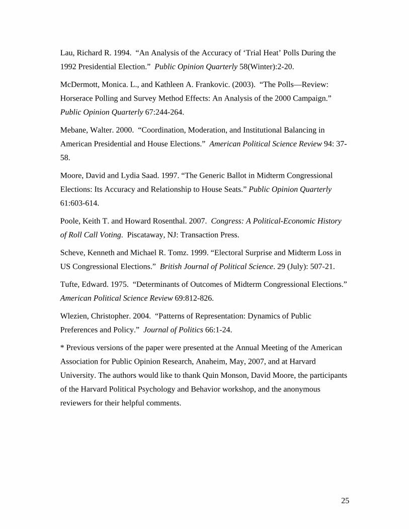
Table 3 returns to the February generic poll results, this time as an independent

variable accounting for the actual November vote. The task is to predict the November

vote from information available in February. Equation 13 shows the “best” equation with

two variables accounting for almost eighty percent of the variance in the vote: the

February generic ballot results plus the current presidential party. No other information

matters—not February party identification, not the lagged congressional vote, not the

lagged presidential vote, and not the lagged presidential party (which, like party

identification, is incorporated in the February generic vote).


Of central interest from equation 13 is the highly significant (.001) coefficient for

the current presidential party. It indicates that which party holds the presidency makes a

11

difference of over five percentage points (-2.65 x 2) beyond the prediction from the

generic polls in February. This differential represents the effect of the campaign between

February and November. Statistically, the predictive power of the presidential party is

equivalent to that of the February generic polls when measured by the difference in t-

values (-5.95 vs. 5.94) or the difference in standardized “beta” coefficients (-0.73 vs.

0.71). To predict the November vote in February, the party of the president is at least as

important as the generic polls. And, as equations 14-17 show, to know only the

president’s party and generic poll results means that other indicators—including party

identification and electoral history—are of little use.

As estimated, the out party gains 5.3 percentage points (2.65 times 2) from

February to November. Since on average a party is only 4.2 percentage points better off

at midterm when it does not hold the presidency, our estimate overshoots the net out-

party advantage. The gap is made up by the fact that in February the out party is

disadvantaged by 1.2 percentage points. (This estimate is obtained by predicting the

expected two-party vote based on February polls but subtracting out the -2.65 presidential

party effect from equation 13.) The next task is to model the vote as a function of the

presidential party plus the generic polls at various time points between February and

November.


Table 4 takes this next step. Equations 18-23 predict the November congressional

vote from the generic polls plus presidential party at each of the six measured mileposts.

They present strong and stable fits with the data. No matter when in the campaign the

generic ballot results are measured, more than three quarters of the variance in the vote

12

can be explained. This stability suggests that partisan preferences are firmly in place by

the onset of the midterm year and captured by the generic polls.11 The equations’

intercepts are consistently small and non-significant, an indication that the generic polls

contain no persistent partisan bias. The coefficients for the generic poll division do not

change with the time of the poll—hovering in the very narrow range between 0.46 and

0.51. Leads at any point in time are effectively halved by Election Day, ceteris paribus.

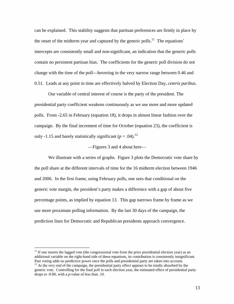
Our variable of central interest of course is the party of the president. The

presidential party coefficient weakens continuously as we use more and more updated

polls. From -2.65 in February (equation 18), it drops in almost linear fashion over the

campaign. By the final increment of time for October (equation 23), the coefficient is

only -1.15 and barely statistically significant (p = .04).12

—Figures 3 and 4 about here—

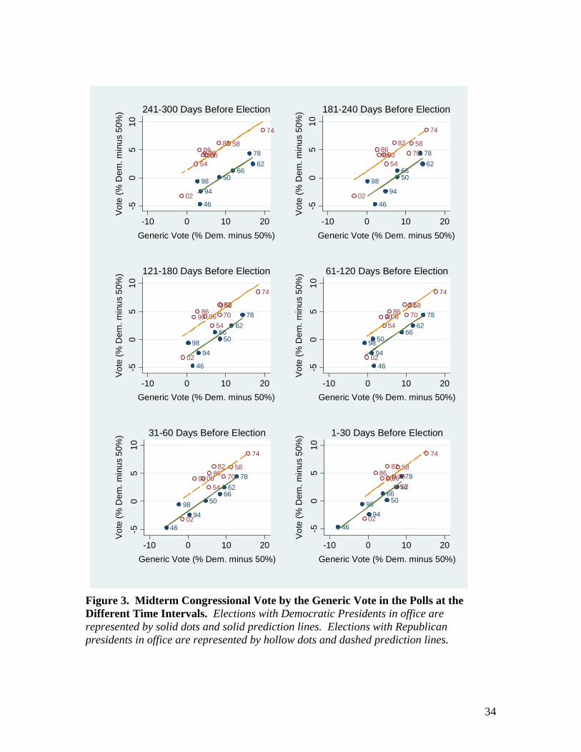
We illustrate with a series of graphs. Figure 3 plots the Democratic vote share by

the poll share at the different intervals of time for the 16 midterm election between 1946

and 2006. In the first frame, using February polls, one sees that conditional on the

generic vote margin, the president’s party makes a difference with a gap of about five

percentage points, as implied by equation 13. This gap narrows frame by frame as we

use more proximate polling information. By the last 30 days of the campaign, the

prediction lines for Democratic and Republican presidents approach convergence.

11 If one inserts the lagged vote (the congressional vote from the prior presidential election year) as an additional variable on the right-hand side of these equations, its contribution is consistently insignificant. Past voting adds no predictive power once the polls and presidential party are taken into account. 12 At the very end of the campaign, the presidential party effect appears to be totally absorbed by the generic vote. Controlling for the final poll in each election year, the estimated effect of presidential party drops to -0.80, with a p-value of less than .10.

13

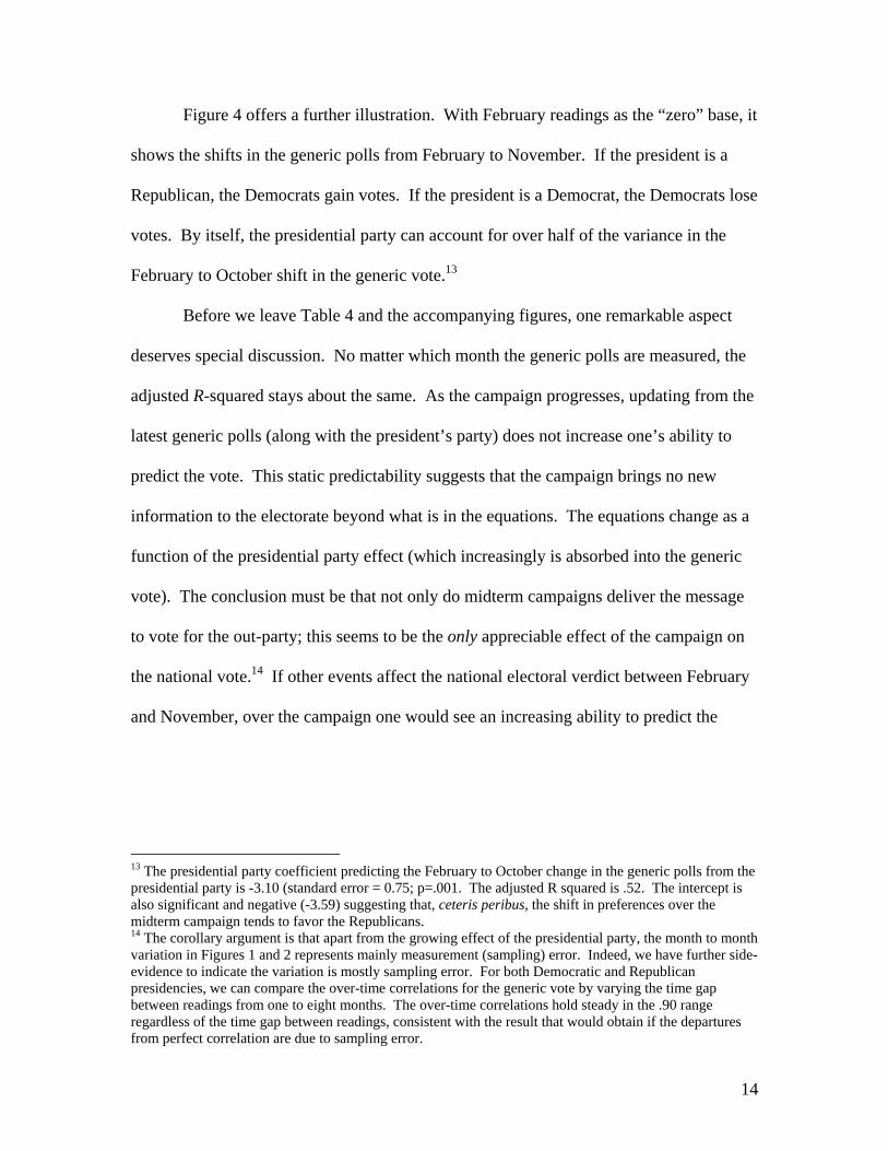
Figure 4 offers a further illustration. With February readings as the “zero” base, it

shows the shifts in the generic polls from February to November. If the president is a

Republican, the Democrats gain votes. If the president is a Democrat, the Democrats lose

votes. By itself, the presidential party can account for over half of the variance in the

February to October shift in the generic vote.13

Before we leave Table 4 and the accompanying figures, one remarkable aspect

deserves special discussion. No matter which month the generic polls are measured, the

adjusted R-squared stays about the same. As the campaign progresses, updating from the

latest generic polls (along with the president’s party) does not increase one’s ability to

predict the vote. This static predictability suggests that the campaign brings no new

information to the electorate beyond what is in the equations. The equations change as a

function of the presidential party effect (which increasingly is absorbed into the generic

vote). The conclusion must be that not only do midterm campaigns deliver the message

to vote for the out-party; this seems to be the only appreciable effect of the campaign on

the national vote.14 If other events affect the national electoral verdict between February

and November, over the campaign one would see an increasing ability to predict the

13 The presidential party coefficient predicting the February to October change in the generic polls from the presidential party is -3.10 (standard error = 0.75; p=.001. The adjusted R squared is .52. The intercept is also significant and negative (-3.59) suggesting that, ceteris peribus, the shift in preferences over the midterm campaign tends to favor the Republicans. 14 The corollary argument is that apart from the growing effect of the presidential party, the month to month variation in Figures 1 and 2 represents mainly measurement (sampling) error. Indeed, we have further side-evidence to indicate the variation is mostly sampling error. For both Democratic and Republican presidencies, we can compare the over-time correlations for the generic vote by varying the time gap between readings from one to eight months. The over-time correlations hold steady in the .90 range regardless of the time gap between readings, consistent with the result that would obtain if the departures from perfect correlation are due to sampling error.

14

election from the latest polls.15 That this does not happen suggests the absence of

unaccounted-for events that affect the vote.16

Summary

This section has analyzed the generic congressional election poll results over 16

midterms. At our first measurement in February we find no evidence of electoral

balancing. As the campaign progresses, the out party gains in the polls and ultimately at

the ballot box. Although involving only a small percent of the electorate, this change is

nearly universal across the sixteen elections. Moreover, the evidence suggests that little

else contributes to change in the national vote.

At the beginning of the election year, voters’ opinions about the upcoming

November election are unformed and do not reflect much consideration of the party of

the president. Over time, as voters begin to focus on the upcoming election, they

increasingly take into account the party of the president. Their increasing attraction to

the out party is the change generated by the midterm campaign. We attribute this shift in

voter sentiment to a growing consideration of the presidential party and the fact that

policy balance can be restored toward the center by electing more members of the

opposition party to Congress. 15 A useful comparison is the ability to predict the vote at various stages of the presidential campaign. As can be seen from Table 4, the root mean squared error (RMSE), is essentially unchanged—for instance 1.83 in April and 1.84 in October. By comparison, if one predicts presidential elections by the trial heat polls in April using the eventual presidential candidates, the RMSE is well over 4 points. If one predicts the presidential vote from trial heat polls from the final week of the campaign, the RMSE is 1.94, which is slightly larger than the prediction error from the midterm generic vote. (This might not be a fair comparison, since the presidential readings include the error-filled 1948 observation. From 1952 onward, the final weeks’ polls predict the vote with considerable precision. The RMSE is a mere 1.37 based on a .95 adjusted R-squared.) This analysis of presidential election polls is based on data compiled by the authors. 16 Suppose we replace the generic vote on the right hand side in Table 4, with its two predictors—current party identification plus the lagged presidential vote. The result is again a stable R squared, averaging .80—slightly higher than in Table 4. With these alternative equations, the presidential vote coefficient is stable from the February to October, which makes sense since partisanship is fairly stable over the campaign interval.

15

The “Negative Referendum” Theory Revisited

TAs an alternative to our account that the electorate learns to vote for the

opposition party in order to restore ideological balance, the rival “negative referendum”

explanation deserves our consideration as an alternative explanation. Does electoral

support for the presidential party sag over the midterm year because voters consider the

policy implications of the presidential party, as we suggest? Or is the declining support

for the presidential party simply due to voters become disillusioned with the presidential

party’s performance at governing, as referendum theory suggests? If presidential support

can account for the slide in the presidential party vote, then it is the public reaction to the

presidential performance rather than the president’s party affiliation that is the cause.

Presidential Approval and Midterm Loss

To test the applicability of referendum theory, we measure political conditions by

the president’s approval rating in the Gallup Poll. We wish to understand the effect of

approval on the vote independent of the trail heat polls. First, we ask, does approval

matter? Table 5 models the midterm vote with presidential approval on the right-hand

side. Approval is measured as the deviation from 50 percent multiplied by the

presidential party dummy variable (+1 if Democrat, -1 if Republican). Choosing 50

percent as the benchmark provides no loss of generality regarding the approval

coefficient, which is a statistically significant 0.16.17 Note, however, that the size of the

presidential party coefficient now becomes conditional on approval at 50 percent.18

17 Unlike presidential approval, economic performance has no clear effect on the midterm vote. We tried two economic measures: (1) the October reading of the consumer sentiment index and (2) growth in per capita disposable income as measured by the Bureau of Economic Analysis. Neither variable (multiplied by presidential party) is significant when added to our models, with or without approval in the equation. 18 The product of presidential approval (minus 50 percent) and the presidential party dummy is an interaction term. The coefficient and standard error are unaffected by the choice of 50 percent as the

16


We can manipulate the presidential party coefficient to become larger or smaller

by moving the benchmark up or down from 50 percent. If we move it up to 65.6 percent,

we make the presidential party effect disappear. This is shown in equation 31, which is

algebraically equivalent to equation 30. The value 65.6 is the crude estimate of the

threshold of approval at which the president must obtain for his party to not be

disadvantaged at midterm.19 If it were the case that presidents typically average about 66

percent approval at midterm, there would be no advantage for being the out party.20

The elemental problem with the negative referendum explanation for midterm

loss is that as measured by presidential approval, presidents are not unusually unpopular

during midterm campaigns. If presidents always wallow at, say, an abnormally low 30

percent approval at midterm, the negative referendum explanation would have bite as the

underlying cause for midterm loss. The average presidential approval in October of

midterm years is 54.1%, virtually identical to the long-term average for all months, 1946-

reference point. We could subtract any amount from the percent approval and obtain the same result. The choice of reference point does, however, affect the coefficients for the additive component, the presidential party. This is why we chose 50 percent since it is a useful, seemingly neutral, reference point. We do not include presidential approval in the equation as an additive term because we assume that the effect of approval is identical for Republican and Democratic presidents. The equations of Table 5 are algebraically equivalent to an alternative equation format where the vote variables are measured as the presidential party vote rather than the Democratic vote where the congressional vote is a function of the lagged vote, the presidential party, and presidential approval. With the alternative format, our usual presidential party effect would be represented by the equation intercept (constant) while our usual intercept (with its trivial value) would be represented by the presidential party coefficient. 19 Only George W. Bush (2002) and Bill Clinton (1998) bested the 65.6 approval benchmark in October of the midterm year. While his rough estimate of 65.6 percent presidential approval is the value that would neutralize the midterm disadvantage for the presidential party, it does not take into account midterm loss from the presidential election. Using equations 30 or 31 as a guide, presidents would need on average around 76 percent approval to overcome both the party’s disadvantage at midterm plus the loss of coattails from the presidential year. 20 With party identification added to the equation, the approval coefficient plunges to 0.08, half its original value. Evidently, to the extent approval affects the midterm vote, it is also absorbed by party identification, which in turn predicts the vote. Since party identification has been central to our modeling all along, its absorbing of approval effects constrains the possibilities of further dynamics involving the president’s approval level

17

2006 (54.7%). Moreover, October approval in midterms averages 3.1 points higher than

in October of the following year and 2.1 points higher than in October of the following

presidential year (two years ahead). Even in the nine instances when the president sought

reelection two years later, the president’s approval averages 1.7 points higher at midterm

than later when seeking reelection (and winning six of nine times).

Presidential Approval and Midterm Year Electoral Change

Even though as a rule the electorate is not particularly dissatisfied with the

president at midterm, one might still argue that the electorate tends to punish the

president’s party at midterm because (for some reason) it sets the performance bar

unusually high at midterm. The obvious challenge to the high-threshold explanation is

that it must account for the fact that the electorate is not inclined to punish the

presidential party at the start of the midterm year. Could dissatisfaction with the

president account for the persistent decline in support for the president’s congressional

party over the midterm year? There are two possible mechanisms.

Most obviously, even though the president’s popularity at midterm is no worse

than average, it could be declining from an earlier high at the start of the midterm year—

perhaps the residual from the initial honeymoon. If so, a demanding electorate could be

satisfied early in the midterm year but then turn sour as the midterm campaign

progresses. Or, even if the president’s perceived performance does not decline over the

election year, it could become an increasingly relevant factor because it becomes

increasingly salient. Just as the campaign could teach the electorate to consider the

policy implications of voting for or against the presidential party, it could teach the

electorate to consider the president’s performance when voting for Congress. A growing

18

focus on presidential performance during the midterm campaign would dispose a

demanding electorate to become increasingly inclined to vote against the president.

First, let us consider the evidence regarding the change in presidential approval

from February (when the poll evidence shows no tendency to punish the presidential

party) to October (when midterm loss is almost fully incorporated in the polls). Over

sixteen midterms, approval declined in nine cases but increases in the other seven. On

average, approval declines a modest 3.4 percentage points from February to October. Is

this sufficient to make a meaningful difference in support for the presidential ticket?21


Table 6 shows some relevant regressions. Equation 32 sets the benchmark,

repeating equation 13 (from Table 3) which predicts the Democratic vote from February

polls and the president’s party. Equation 33 adds the February to October shift in

presidential approval times presidential party (+1=Dem, -1=Rep). The coefficient of 0.04

for approval change is small and non-significant, and it hardly detracts from the

presidential party effect (coefficients of -2.65 versus -2.55). Clearly, knowing in

February the upcoming trend in presidential approval would not help one predict the

November election. This result refutes the idea that declining presidential approval over

the midterm year generates the evolving rejection of the presidential party.22

21 We can also examine the change in the economy over the midterm year. Over 15 observations of change from quarter 1 to quarter 3 of midterm years, per capita real income growth rose in 11 years and fell in four. For 14 observations of consumer sentiment from quarter 1 to quarter 3, sentiment rose in 3 but fell in the other 11. The mean change, however, was a trivial 3 out of 200 points. 22 It might seem that a useful test would be to regress change in the generic vote on change in presidential approval. A problem arises, however, with the two change variables measured for the same time interval; given that the two measures share some of the same respondents, they share sampling error. (For example, an unusually Republican sample at time 2 would have an artificially pro-Republican generic vote and an artificially pro-Republican approval score.) Comparing October to February readings, the regression of change in the generic vote on the change in approval is 0.24, with a significant .01 p-values. However, this correlation suffers from the correlated errors problem mentioned above. A better test is to relate change in

19

Still, a possible “out” for the high-threshold explanation is that, just as with the

“balancing” explanation, the electorate does not incorporate thinking about the

president’s job performance until late in the campaign. To test this idea, equation 34

regresses the November vote on February generic polls, the presidential party, and

February approval. The test is whether approval’s entry in the equation diminishes the

presidential party effect. Clearly it does not. Knowing the president’s standing with the

public in February has no bearing on the midterm election year trajectory of the vote

beyond what the equation’s other variables reveal; the presidential party effect holds firm

with February approval controlled. Equation 35 substitutes October approval for

February approval. Again the coefficient is not significant and there is no impact on the

other terms of the equation. Knowing in February of the midterm year how the president

will stand with the public in October has little bearing on the trajectory of preferences

over the campaign. As before, the key predictor is the party of the president.23

The remarkable aspect of equation 35 is that the effect of presidential approval as

measured in October is already mainly absorbed by polls as measured in February. The

president’s standing in the polls does not change much over the midterm year and when it

does change it is not clear that it matters much since the vote, apart from the impact of

the generic vote from April to October on change in approval from February to August. Here, the two measures are from different sets of time points, thus not sharing sampling error. The regression coefficient now drops to 0.06, with a .p-value of .43. 23 As a further test, we can predict the “vote” in generic polls, February to October, and observe whether the coefficient for approval changes. When the equations of Table 2 are replicated with the addition of either current or lagged (one month) presidential approval, the coefficients are always small and not significant. Seemingly, the effects of presidential approval are largely absorbed by current party identification. The approval coefficients do not increase with time. If anything the coefficients decline over time. For instance, using current approval, the trivial coefficients are 0.06 for February and -0.03 for October. When party identification is omitted from these equations, the coefficient for current approval declines from a significant 0.19 in February to a nonsignificant 0.13 in October. Using lagged approval the decline is from 0.22 (February) to 0.10 (October). Clearly there is no evidence that generic poll respondents increasingly take their evaluations of the president into account when casting hypothetical congressional ballots.

20

the presidential party, is fairly well set by February. The one change in every midterm

campaign is the growing negative impact of the president’s party.

Summary

This section has tested the hypothesis that the presidential party’s negative

trajectory at midterm is due to voters reacting negatively to the president’s performance.

While the national vote is affected by the president’s approval rating, presidents are not

unusually unpopular at midterm. And the pattern of decline in presidential popularity

over the midterm year is too small and ragged to account for the negative shift.

Moreover, there is no evidence that the president’s popularity becomes a more salient

factor over the midterm campaign. In short, we find no empirical support for the idea

that the midterm sag in electoral fortunes of congressional candidates of the presidential

party is the product of a negative referendum on presidential performance.

Discussion and Conclusion

The pattern of midterm loss for the presidential party is a function of an advantage

for the winning party in the presidential election followed by an advantage for the losing

party at the subsequent midterm. While much attention has focused on the former

phenomenon, the latter is actually of greater magnitude, as parties typically gain more at

midterm by losing the presidential election than they gain from winning the presidency.

This paper has focused on the trends in partisan vote preference over the sixteen most

recent midterm years. We do not challenge the presence of a presidential year surge or

coattails and their withdrawal as part of the explanation. Our search has been for the

component of midterm loss that results from the behavior of voters in the midterm year.

21

The main contribution of this paper derives from our exploitation of “generic

ballot” polls for midterm congressional elections. . Early in the campaign, voters tell

pollsters their party choice without much thought beyond the immediate political

environment. The electorate's vote trajectory over the campaign is toward the out party,

as if the value of balance becomes clear once the voters focus on their November

decision.24

Our results do not mean that the midterm vote is unaffected by the president’s

popularity, as we have shown that it is. They do mean that the effects are already largely

absorbed in the generic polls as of February of the election year. Between February and

Election Day, the presidential party’s vote strength almost always declines, and the

degree of decline is unrelated to the public’s evaluation of the president. Clearly, during

the midterm election year, the electorate shifts away from the presidential party in its vote

choice for reasons that have nothing to do with the electorate’s attitudes toward the

president. By default, this is balancing: the electorate votes against the presidential party

to give more power to the other party, but does not incorporate this motivation in its

thinking until Election Day approaches.

The alternative interpretation of our findings is that midterm voters simply turn

negative against the incumbent president as if for no reason although this bias against the

sitting president is absent at other times, not even in the Spring of the midterm year. We

prefer a purpose-driven explanation: a desire to balance the policies of the parties. We

often find resistance to this idea on the grounds that it taxes the cognitive capability of

24 The results are at least as strong if not stronger if we substitute the two-party division of House seats for the two-party vote in the various equations. The results also hold for the partisan division of Senate seats up for election.

22

ordinary voters. But all that is required is that some voters know and care about the

parties’ policy tendencies and also know which party holds the presidency.25

We end up with two separate but compatible explanations for midterm loss. In

presidential years, the winning presidential party is advantaged in the congressional

elections, due to the surge/coattails phenomenon. As we have examined here, at

midterm the presidential party is disadvantaged, as the electorate shifts its preferences to

the out party. Together these two components generate the regularity of midterm loss.

25. Some will say that our theory of a policy-driven motivation requires testing with survey respondents as opposed to mere aggregates of actual voters. What this test should be is not clear, as the independent variable known as the president’s party is common knowledge to all. One might pursue whether voting against the presidential party is most frequent among certain types of voters more than others, such as those who appear more politically knowledgeable, a group more likely to take policy considerations into accounts. Evidence that voters chose based on their own ideology would be consistent with balancing behavior but also with issue voting that ignores the presidential party. The value of survey analysis is limited, by the fact that the presidential penalty at midterm is only a few percentage points. While a differential of this size appears large in the context of aggregate analysis, searching for a difference of a few percentage points is like looking for a needle in a haystack at the individual level.

23

References

Abramowitz, Alan, Alan Cover, and Helmut Norpoth. 1986. “The President’s Party in

Midterm Elections: Going from Bad to Worse.“ American Journal of Political Science.

33(3): 562-76.

Alesina, Roberto and Howard Rosenthal. 1995. Partisan Politics, Divided Government,

and the Economy. New York: Cambridge University Press.

Bafumi, Joseph and Michael Herron. 2007. “Preference Aggregation, Representation, and

Elected American Political Institutions”. Unpublished Manuscript.

Campbell, Angus. 1966. "Surge and Decline: A Study of Electoral Change." In Angus

Campbell, Philip E. Converse, Warren E. Miller and Donald E. Stokes (eds.), Elections

and the Political Order. New York: Wiley, pps 40-62

Campbell, James E. 1997. The Presidential Pulse of Congressional Elections.

Lexington: University of Kentucky Press.

Erikson, Robert S., Michael B. MacKuen, and James A. Stimson. 2002. The

Macropolity. Cambridge: Cambridge University Press.

Erikson, Robert S. and Lee Sigelman. 1995. "Poll-Based Forecasts of Midterm

Congressional Elections: Do the Pollsters Get it Right?" Public Opinion Quarterly 59:

Winter 1995, 589-605.

Fiorina, Morris. P. 2003. Divided Govenrment. 2nd. Ed. New York: Longman.

Jacobson, C. Gary. 2004. The Politics of Congressional Elections. 6th ed. New York:

Longman.

Jacobson, C. Gary and Samuel Kernell. 1983. Strategy and Choice in Congressional

Elections. New Haven: Yale University Press.

Kernell, Samuel. 1977. “Presidential Popularity and Negative Voting.” American

Political Science Review 71: 44-66.

24

Lau, Richard R. 1994. “An Analysis of the Accuracy of ‘Trial Heat’ Polls During the

1992 Presidential Election.” Public Opinion Quarterly 58(Winter):2-20.

McDermott, Monica. L., and Kathleen A. Frankovic. (2003). “The Polls—Review:

Horserace Polling and Survey Method Effects: An Analysis of the 2000 Campaign.”

Public Opinion Quarterly 67:244-264.

Mebane, Walter. 2000. “Coordination, Moderation, and Institutional Balancing in

American Presidential and House Elections.” American Political Science Review 94: 37-

58.

Moore, David and Lydia Saad. 1997. “The Generic Ballot in Midterm Congressional

Elections: Its Accuracy and Relationship to House Seats.” Public Opinion Quarterly

61:603-614.

Poole, Keith T. and Howard Rosenthal. 2007. Congress: A Political-Economic History

of Roll Call Voting. Piscataway, NJ: Transaction Press.

Scheve, Kenneth and Michael R. Tomz. 1999. “Electoral Surprise and Midterm Loss in

US Congressional Elections.” British Journal of Political Science. 29 (July): 507-21.

Tufte, Edward. 1975. “Determinants of Outcomes of Midterm Congressional Elections.”

American Political Science Review 69:812-826.

Wlezien, Christopher. 2004. “Patterns of Representation: Dynamics of Public

Preferences and Policy.” Journal of Politics 66:1-24.

* Previous versions of the paper were presented at the Annual Meeting of the American

Association for Public Opinion Research, Anaheim, May, 2007, and at Harvard

University. The authors would like to thank Quin Monson, David Moore, the participants

of the Harvard Political Psychology and Behavior workshop, and the anonymous

reviewers for their helpful comments.

25

Table 1. FEBRUARY POLLS. Predicting the Generic Vote in February Polls, 16 Midterm Years 1946-2006

Dependent Variable = February Generic Poll Results (% Dem. minus 50%)

(1) (2) (3) (4) (5)

Party Identification in February (% Dem. minus 50%)

0.72 (0.08)***

0.71 (0.08)***

0.66 (0.09)***

0.72 (0.08)***

0.66 (0.11)***

Lagged Presidential Party (1=D, -1=R.)

-2.31 (0.53)***

-2.35 (0.54)***

-2.14 (0.52)**

-2.49 (0.59)***

-2.14 (0.77)*

Current Presidential Party (1=D, -1=R.)

0.27 (0.57)

-0.24 (1.08)

Lagged Congressional Vote (% Dem. minus 50%)

0.33 (0.25)

0.36 (0.34)

Lagged Presidential Vote (% Dem. minus 50%)

0.07 (0.10)

0.02 (0.21)

Intercept 0.74 (0.88)

0.88 (0.95)

0.50 (0.88)

0.80 (0.91)

0.38 (1.08)

Adjusted R squared .88 .87 .89 .87 .87

RMSE 2.08 2.15 2.03 2.13 2.21

Note: “February” polls actually represent polls from 241 to 300 days in advance of the election. Generic poll results and all vote variables are measured as the Democratic percent of the two-party vote minus 50 percent. Party identification is measured as the Democratic percent of Democratic or Republican partisans, minus 50 percent. * p < .05, ** p < .01, *** p < .001

26

Table 2. THE GENERIC VOTE AT VARIOUS STAGES OF THE CAMPAIGN. Predicting Generic Ballot Poll Results at Different Time Intervals from Party Identification and the Presidential Party,

16 midterm elections, 1946-2006.

Dependent Variable = Generic Poll Results (% Dem. minus 50%) (6) (7) (8) (9) (10) (11) (12)

241-300 Days Out

(Feb.)

181-240 Days Out

(April)

121-180 Days Out

(June)

61-120 Days Out

(August)

31-60 Days Out

(Sept.)

1-30 Days Out

(Oct.)

Election Day Vote (Nov.)

Party Identification (% Dem. minus 50%)

0.71 (0.08)***

0.77 (0.12)***

0.91 (0.09)***

0.86 (0.10)***

0.83 (0.06)***

0.73 (0.06)***

0.39 (0.07)***

Lagged Presidential Party (1=D, -1=R)

-2.35 (0.54)***

-1.15 (0.66)

-0.93 (0.47)

-1.78 (0.53)**

-2.25 (0.37)***

-1.57 (0.36)***

-1.25 (0.40)**


0.27 (0.57)

-0.07 (0.66)

-0.64 (0.48)

-1.62 (0.55)*

-1.90 (0.38)***

-1.56 (0.36)***

-1.89 (0.40)***

Intercept 0.88 (0.95)

0.55 (1.16)

-0.46 (0.86)

-0.84 (1.02)

-1.59 (0.64)*

-1.04 (0.70)

-1.04 (0.70)

Adj. R2 .87 .77 .88 .85 .93 .93 .82

Root MSE 2.15 2.56 1.86 2.12 1.49 1.43 1.59

Note: Generic poll results are measured as the Democratic percent of the two-party vote minus 50 percent. Party identification is measured as the Democratic percent of Democratic or Republican partisans, minus 50 percent. Party identification is measured for the indicated month except that for predicting the actual vote, party i.d. in October (rather than November) is used. Equation 6 is a repeat of equation 2 from Table 1. * p < .05, ** p < .01, *** p < .001

27

Table 3. FROM FEBRUARY TO ELECTION DAY. Predicting the Midterm Congressional Vote from Generic Vote in February Polls plus other Variables, 16 midterm Years 1946-2006

Dependent Variable = Democratic % of Actual Two–Party Vote in November, minus 50%

(13) (14) (15) (16) (17)

February Generic Poll Results (% Dem. minus 50%)

0.44 (0.08)***

0.37 (0.15)*

0.41 (0.10)***

0.42 (0.09)***

0.42 (0.09)***

Party Identification in February (% Dem. minus 50%)

0.08 (0.13)

Lagged Presidential Party (1=D, -1=R.)

-0.28 (0.50)


-2.65 (0.45)***

-2.70 (0.46)***

-2.80 (0.54)***

-2.58 (0.47)***

-2.83 (0.83)*

Lagged Congressional Vote (% Dem. minus 50%)

0.15 (0.27)

Lagged Presidential Vote (% Dem. minus 50%)

-0.07 (0.14)

Intercept -1.26 (0.72)

-1.42 (0.79)

-1.39 (0.78)

-1.05 (1.62)

-1.13 (0.80)

Adjusted R squared .78 .77 .77 .77 .77

RMSE 1.72 1.77 1.77 1.77 1.77

Note: “February” polls actually represent polls from 241 to 300 days in advance of the election. Generic poll results and all vote variables are measured as the Democratic percent of the two-party vote minus 50 percent. Party identification is measured as the Democratic percent of Democratic or Republican partisans, minus 50 percent. *p<.05.**p<.01,***p<.001.

28

Table 4. CAMPAIGN DYNAMICS OVER VARYING TIME INTERVALS. Predicting Midterm Congressional Vote from the Generic Ballot Poll Results at different times

plus Presidential Party, 16 midterm elections 1946-2006 Dependent Variable = Democratic % of Actual Two–Party Vote in November, minus 50%

(18) (19) (20) (21) (22) (23)

241-300 Days Out

(Feb.)

181-240 Days Out

(April)

121-180 Days Out

(June)

61-120 Days Out

(August)

31-60 Days Out

(Sept.)

1-30 Days Out

(Oct.)

Generic Poll Results (% Dem. minus 50%)

0.44*** (0.08)

0.48*** (0.09)

0.48*** (0.09)

0.47*** (0.09)

0.47*** (0.07)

0.52*** (0.10)

Current Presidential Party (R=-1, D=+1)

-2.65*** (0.45)

-2.29*** (0.46)

-2.07*** (0.48)

-1.60** (0.46)

-1.45** (0.42)

-1.15* (0.49)


-1.10 (0.75)

-1.00 (0.78)

-0.91 (0.71)

-0.31 (0.56)

0.05 (0.61)

Adj. R2 .78 .76 .74 .76 .81 .75

Root MSE 1.72 1.82 1.89 1.80 1.61 1.84

Note: Generic poll results and the vote are measured as the Democratic percent of the two-party vote minus 50 percent. Equation 18 is a repeat of equation 13 in Table 3. * p < .05, ** p < .01, *** p < .001

29

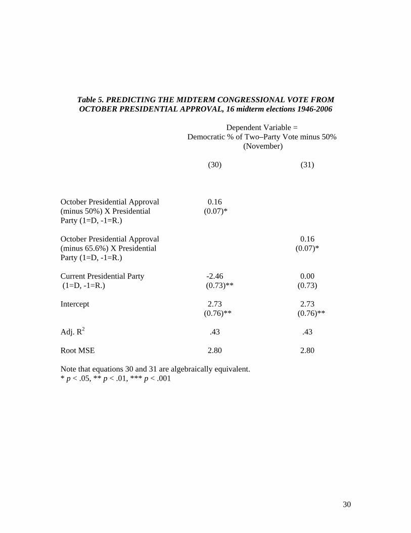
Table 5. PREDICTING THE MIDTERM CONGRESSIONAL VOTE FROM OCTOBER PRESIDENTIAL APPROVAL, 16 midterm elections 1946-2006

Dependent Variable =

Democratic % of Two–Party Vote minus 50% (November)

(30) (31)

October Presidential Approval (minus 50%) X Presidential Party (1=D, -1=R.)

0.16 (0.07)*

October Presidential Approval (minus 65.6%) X Presidential Party (1=D, -1=R.)

0.16 (0.07)*


-2.46 (0.73)**

0.00 (0.73)

Intercept

2.73 (0.76)**

2.73 (0.76)**

Adj. R2 .43 .43

Root MSE 2.80 2.80

Note that equations 30 and 31 are algebraically equivalent. * p < .05, ** p < .01, *** p < .001

30

Table 6. PREDICTING THE VOTE FROM PRESIDENTIAL APPROVAL, 16 midterm elections 1946-2006

Dependent Variable =

Democratic % of Two–Party Vote minus 50% (November)

(32) (33) (34) (35)

February Generic Poll Results (% Dem. minus 50%)

0.44 (0.08)***

0.49 (0.10)***

0.40 (0.10)***

0.40 (0.07)***

Change in Approval (Feb. to Oct.). X Pres. Party

0.04 (0.06)

February Presidential Approval (minus 50) X Pres. Party (1=D, -1=R.)

0.03 (0.04)

October Presidential Approval (minus 50) X Pres. Party (1=D, -1=R.)

0.08 (0.04)


-2.65 (0.45)***

-2.56 (-.47)***

-2.76 (0.48)***

-2.79 (0.42)***


-1.47 (0.79)

-0.91 (0.88)

0.61 (0.76)

Adjusted R squared .78 .78 .78 .82

RMSE 1.72 1.75 1.75 1.59

Note: Poll results and the vote are measured as the Democratic percent of the two-party vote minus 50 percent.

31

Figure 1. Midterm Loss as the Subtraction of the Presidential Year Vote from the Midterm Year Vote, 1944-46—2004-06.

32

-3 -2 -1 0 1 2 3

Ideological Position

Bush

110th House

Median Voter

109th House

Figure 2. The Ideological Positions of the House, President and Voters on a Common Scale. Ideal points based on roll call data and CCES survey interviews. House ideal points represent the median member. Source: Adopted from Bafumi and Herron, “Preference Aggregation, Representation, and Elected American Political Institutions.” Unpublished Manuscript.

33

46

50

6266

78

9498

54

5870

74

828690

02

06

-50

510

Vote

(% D

em. m

inus

50%

)

-10 0 10 20Generic Vote (% Dem. minus 50%)

241-300 Days Before Election

46

50

6266

78

9498

54

5870

74

8286

90

02

06

-50

510

Vote

(% D

em. m

inus

50%

)



46

50

6266

78

9498

54

5870

74

8286

90

02

06

-50

510

Vote

(% D

em. m

inus

50%

)



46

50

6266

78

9498

54

5870

74

8286

90

02

06-5

05

10Vo

te (%

Dem

. min

us 5

0%)



46

50

6266

78

9498

54

5870

74

8286

90

02

06

-50

510

Vot

e (%

Dem

. min

us 5

0%)



46

50

6266

78

9498

54

5870

74

8286

90

02

06

-50

510

Vot

e (%

Dem

. min

us 5

0%)



Figure 3. Midterm Congressional Vote by the Generic Vote in the Polls at the Different Time Intervals. Elections with Democratic Presidents in office are represented by solid dots and solid prediction lines. Elections with Republican presidents in office are represented by hollow dots and dashed prediction lines.

34

1946

1950

1962

19661978

19941998

1954

1958

1970

1974

1982

19861990

20022006

-10

-50

510

2 4 6 8 10 12Month

Cha

nge

in D

emoc

ratic

Vot

e

Figure 4. Net Change in the generic congressional vote (Percent Democratic), February to October, relative to February as the starting point. Dashed lines indicate midterm years with Republican presidents. Solid lines indicate midterm years with Democratic presidents.

35

Documents

Joseph Bafumi,a Robert S. Erikson,b and Christopher Wlezienc