Joint Vanishing Point Extraction and Tracking

Till Kroeger1 Dengxin Dai1 Luc Van Gool1,2

1Computer Vision Laboratory, D-ITET, ETH Zurich2VISICS, ESAT/PSI, KU Leuven

{kroegert, dai, vangool}@vision.ee.ethz.ch

Abstract

We present a novel vanishing point (VP) detection andtracking algorithm for calibrated monocular image se-quences. Previous VP detection and tracking methods usu-ally assume known camera poses for all frames or detectand track separately. We advance the state-of-the-art bycombining VP extraction on a Gaussian sphere with re-cent advances in multi-target tracking on probabilistic oc-cupancy fields. The solution is obtained by solving a LinearProgram (LP). This enables the joint detection and track-ing of multiple VPs over sequences. Unlike existing workswe do not need known camera poses, and at the same timeavoid detecting and tracking in separate steps. We also pro-pose an extension to enforce VP orthogonality. We augmentan existing video dataset consisting of 48 monocular videoswith multiple annotated VPs in 14448 frames for evalua-tion. Although the method is designed for unknown cameraposes, it is also helpful in scenarios with known poses, sincea multi-frame approach in VP detection helps to regularizein frames with weak VP line support.

1. IntroductionA vanishing point (VP) is the point of convergence of a

set of parallel lines in the imaged scene under a projectivetransformation. Man-made structures often consist of geo-metric primitives, such as multiple sets of parallel or orthog-onal planes and lines in the scene. Because of this, the de-tection of projected VPs in images provides strong cues forthe extraction of knowledge about the unknown 3D worldstructure. VPs can often be further constrained to mutualorthogonality, due to the preference of right angles in man-made structures. Detected VPs have been used as a low-level input to many higher-level computer vision tasks, suchas 3D reconstruction [9, 14], autonomous navigation [23],camera calibration [12, 33] and pose estimation [15, 22].

Many applications, which take video sequences or un-ordered image sets as input, require VP estimates in ev-ery frame and VP identities across views or frames. Usu-

Figure 1: Tracked vanishing directions are shown together withassociated imaged line segments in three frames of a sequence.This and the subsequent figures are best viewed in color.

ally, when this is needed, the camera pose is assumed to beknown for every frame [1, 13], thereby rendering the VPassociation across images simple, or separate steps for VPdetection and tracking (particle filters [23, 25], greedy as-signment [11]) are used. Since pose knowledge can onlybe obtained through expensive odometry or external mo-tion measurements, it will often not be available. SeparateVP detection and tracking often results in missed detectionsor loss and re-initialization of VP tracks due to weak linesupport in some frames. Even in the case of known poses,joint detection over multiple frames benefits from integrat-ing image evidence of many frames. Joint reasoning oversequences is particularly useful if long-term VP identitiesare required, and re-initializations are expensive.

To the best of our knowledge, no method exists thatjointly extracts multiple VPs in all frames of a video withunknown camera motion. Our contributions are twofold:

1. Method. We propose the first algorithm for the jointVP extraction over all images of a sequence with unknowncamera poses. We borrow from recent advances in multi-target tracking [6, 35] and model the problem as a variantof a network-flow tracking problem. We compute line seg-ments in each frame and discretize the set of possible VPson a probabilistic spherical occupancy grid. Line-VP as-sociation probabilities and VP transition probabilities areconverted into an acyclic graph for joint VP extraction andtracking. VPs are extracted by Linear Programming (LP).

2. Dataset. As the field lacks a dataset for the evaluation

1

of VP extraction in videos, we augmented the Street-Viewvideo dataset of [17] with annotated VPs, which will bepublicly available. We evaluate our approach on this datasetusing established multi-object tracking metrics [7, 19] forunknown camera poses. We chose this dataset because cam-era poses are available for all frames, which enables oneadditional experiment: We evaluate the improvement of ouralgorithm when camera pose information is incorporated.Since our method also works for single frames and orthog-onal VPs, we compare to a recent method[29] for VP detec-tion in Manhattan Scenes on the York Urban Dataset [10].

The paper is organized as follows: §2 introduces our VPparametrization. §3 describes the method, with LP formu-lation in §3.1, and score modeling in §3.2. We evaluate in§4 and conclude in §5 with a discussion of future work.

Related Work

VP extraction has been studied extensively in ComputerVision. The most relevant recent works can be categorizedaccording to several algorithmic design choices:

Input: While some approaches start directly from con-tinuous image gradients or texture [23, 25, 27] and thresh-olded edges images [30], most works rely on short line seg-ments [2, 3, 12, 13, 21, 26, 29, 33], or full lines [8, 11]. If the3D geometry is known, surface normals can be used [28].

Accumulator Space: Intersections of imaged lines canbe computed in the original (unbounded) image space [2,11, 26, 27, 29, 34] or on a (bounded) Gaussian unit sphere,first proposed in [3] and used in [1, 5, 12, 13, 15, 20, 21,22, 24, 28]. We use the latter approach, explained in §2. Itallows for easy discretization [3, 20, 21]. [18] proposes aline parametrization in parallel coordinates to extract VPs.

Line-VP Consistency and VP Refinement: Consis-tency between an estimated VP and image lines can becomputed directly by measuring line endpoint distances inthe image [2, 5, 13, 18, 29], angular differences in the im-age [10, 26], with explicit probabilistic modeling of the lineendpoint errors [34], or with angles between normals of in-terpretation planes in the Gaussian sphere, used by us and[20, 21, 24]. VP computation or refinement with given as-sociated lines is done via Hough voting and non-maximumsuppression [20, 21, 23, 31, 24], solving a quadratic pro-gram [2], implicitly in an EM setting [1, 27, 29, 34], or bylinear least-squares, as in this paper and [15].

Solution: Several different methods exist for combininginput, accumulator space and line-VP consistency measuresinto a final extraction solution. If no discretization of theaccumulator space is attempted, solutions are found withefficient search [10, 26], direct clustering [18, 29], multi-line RANSAC [5, 33], EM procedures [1, 13, 15, 27, 34],or MCMC inference [28]. With a discretized accumulatorspace solutions are found by voting schemes [20, 21, 23, 24]or inference in graphical models [2, 30].

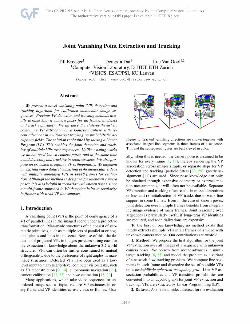
Figure 2: Imaged line segments l1,l2 of scene parallel lines l1,l2 form a VP V2D on the image plane π. The same VP can beparametrized as the vector V3D pointing towards the intersectionof interpretation planes P1, P2 of lines l1, l2 and the unit sphere.

Camera Calibration and VP Orthogonality: Some VPextraction methods assume known internal camera calibra-tion [11, 13, 20, 23, 24, 25]. Others do not need calibra-tion [2, 15, 21, 26, 34]. Internal parameters can be esti-mated from extracted VPs [8, 12, 33]. VPs have also beenused for estimation of external camera parameters: orienta-tion of camera to scene [4, 15], 3D shape to camera [3], andas additional constraints for full camera poses [22]. Often,further scene-dependent VP constraints are included: mu-tual VP orthogonality (Manhattan World) [10, 11, 13, 33],sets of mutually orthogonal VPs [28, 16], with a shared ver-tical VP (Atlanta World) [2, 27].

Multi-View Extraction and VP Tracking: [1] solvesmulti-view VP extraction by Hough voting with EM re-finement, but requires known camera poses. [13] extractsorthogonal VPs independently in multiple views, and inte-grates information across views by using SfM (Structure-from-Motion) camera pose estimates. [11, 16] explicitlytrack orthogonal VPs in videos. [11] extracts VPs sepa-rately in each frame, and greedily links VPs across frames.[16] uses a multi-target tracking approach to link multiplehypothesized sets of mutually orthogonal VPs, but, in con-trast to this work, requires pre-processing to extract can-didates. [23, 25] track VPs for road direction finding. Onefinite horizontal VP, corresponding to the heading direction,is extracted in each frame and tracked using particle filters.

In contrast to these approaches, in our method we finda jointly optimal solution without any knowledge about thecamera pose, or number or relative directions of the VPs.

2. VP RepresentationA 2D VP is the intersection of (the unbounded continua-

tion of) two 2D line segments, imaged from two 3D scene-parallel lines. In Fig. 2 imaged line segments l1, l2 of sceneparallel lines l1, l2 form a VP V2D on the image plane π.The 2D VP may lie inside or outside the image frustum ofπ, or at infinity, in cases when imaged lines remain parallel.

An alternative parametrization, proposed in [3], modelsVP locations on the unit sphere. A point x in homoge-neous image coordinates is normalized by x = K−1x, with

0

0

0

0

0

0

0

0

0

0

0

50

100

150

200

250

300

350

400

450

0

50

100

150

200

250

300

350

400

450Frame 1 Frame 2 Frame 3

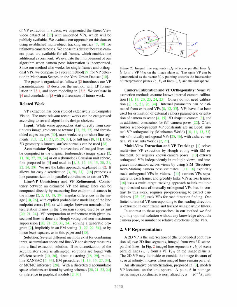
Figure 3: Combined figure for § 2.1 and § 3. For § 2.1: interpreta-tion planes on a discretized sphere for a rotating cube. For visual-ization purposes only four planes belonging to one horizontal VPare drawn. For § 3: directed acyclic graph with, 1) arcs betweenVP bin and Start and T erminal node (blue,cyan), 2) transitionarcs from each VP bin to all bins in following frame (green), 3)line association arcs from each VP bin to all line segments at timet (magenta). For visualization only a subset of all arcs is drawn.

K the camera calibration matrix. A plane P is spannedby the center of projection at [0, 0, 0]T , and the endpointsx1, x2 in normalized homogeneous image coordinates ofan imaged line segment l. The plane is computed as P =x1×x2/(‖x1‖ ‖x2‖), and is called interpretation plane. Forline segments l1, l2, interpretation planes P1, P2 are shownas intersection circles of the planes and the unit sphere inFig. 2. The VP is given as their intersection on the sphere:V3D = ±P1×P2. In the following we use vanishing direc-tion and vanishing point interchangeably. If more than twoplanes are detected, the VP is given by the least-squares so-lution to a system of incidence equations:∑

i< Pi, V3D >= 0 . (1)

2.1. VP Discretization

In order to use the proposed parametrization for trackingwe need to discretize the solution space of possible VPs.Fig. 3 illustrates the chosen discretization: a simple trian-gular tessellation of the sphere by iterative subdivisions ofthe faces of an icosahedron. Three frames of a sequence ofa rotating cube are shown (top row). For visualization pur-poses four line segments belonging to one horizontal VPare drawn in red. With known internal camera calibrationK, four interpretation planes are computed and plotted to-gether with the discretized unit sphere (bottom row). Thered color strength illustrates the likelihood of a VP in eachcell of the spherical grid. This is determined by summingup all line-VP consistency scores as described later in Eq.(14). Since the cube is rotating around a vertical axis, thehorizontal VP rotates accordingly, which can be seen by thechange in VP likelihoods on the spherical grid. Note that the

Frame 3Frame 1 Frame 2

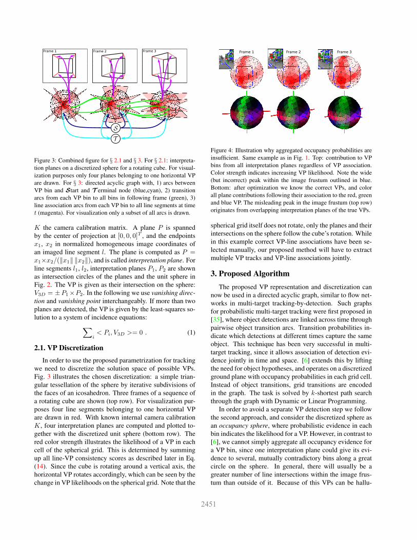
Figure 4: Illustration why aggregated occupancy probabilities areinsufficient. Same example as in Fig. 1. Top: contribution to VPbins from all interpretation planes regardless of VP association.Color strength indicates increasing VP likelihood. Note the wide(but incorrect) peak within the image frustum outlined in blue.Bottom: after optimization we know the correct VPs, and colorall plane contributions following their association to the red, greenand blue VP. The misleading peak in the image frustum (top row)originates from overlapping interpretation planes of the true VPs.

spherical grid itself does not rotate, only the planes and theirintersections on the sphere follow the cube’s rotation. Whilein this example correct VP-line associations have been se-lected manually, our proposed method will have to extractmultiple VP tracks and VP-line associations jointly.

3. Proposed AlgorithmThe proposed VP representation and discretization can

now be used in a directed acyclic graph, similar to flow net-works in multi-target tracking-by-detection. Such graphsfor probabilistic multi-target tracking were first proposed in[35], where object detections are linked across time throughpairwise object transition arcs. Transition probabilities in-dicate which detections at different times capture the sameobject. This technique has been very successful in multi-target tracking, since it allows association of detection evi-dence jointly in time and space. [6] extends this by liftingthe need for object hypotheses, and operates on a discretizedground plane with occupancy probabilities in each grid cell.Instead of object transitions, grid transitions are encodedin the graph. The task is solved by k-shortest path searchthrough the graph with Dynamic or Linear Programming.

In order to avoid a separate VP detection step we followthe second approach, and consider the discretized sphere asan occupancy sphere, where probabilistic evidence in eachbin indicates the likelihood for a VP. However, in contrast to[6], we cannot simply aggregate all occupancy evidence fora VP bin, since one interpretation plane could give its evi-dence to several, mutually contradictory bins along a greatcircle on the sphere. In general, there will usually be agreater number of line intersections within the image frus-tum than outside of it. Because of this VPs can be hallu-

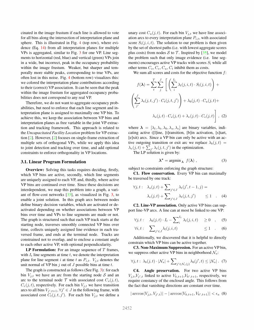
cinated in the image frustum if each line is allowed to votefor all bins along the intersection of interpretation plane andsphere. This is illustrated in Fig. 4 (top row), where evi-dence (Eq. 14) from all interpretation planes for multipleVPs is aggregated, similar to Fig. 3 for one VP. Line seg-ments to horizontal (red, blue) and vertical (green) VPs joinin a wide, but incorrect, peak in the occupancy probabilitywithin the image frustum. Weaker, but sharper and tem-porally more stable peaks, corresponding to true VPs, areoften lost in this noise. Fig. 4 (bottom row) visualizes this:we colored the interpretation plane contributions accordingto their (correct) VP association. It can be seen that the peakwithin the image frustum for aggregated occupancy proba-bilities does not correspond to any real VP.

Therefore, we do not want to aggregate occupancy prob-abilities, but need to enforce that each line segment and in-terpretation plane is assigned to maximally one VP bin. Toachieve this, we keep the association between VP bins andinterpretation planes as free variable in the joint VP extrac-tion and tracking framework. This approach is related tothe Uncapacitated Facility Location problem for VP extrac-tion [2]. However, [2] focuses on single-frame extraction ofmultiple sets of orthogonal VPs, while we apply this ideato joint detection and tracking over time, and add optionalconstraints to enforce orthogonality in VP locations.

3.1. Linear Program Formulation

Overview: Solving this tasks requires deciding, firstly,which VP bins are active, secondly, which line segmentsare uniquely assigned to each VP, and, thirdly, where activeVP bins are continued over time. Since these decisions areinterdependent, we map this problem into a graph, a vari-ant of flow-cost networks [35], as visualized in Fig. 3, toenable a joint solution. In this graph arcs between nodesdefine binary decision variables, which are activated or de-activated depending on whether associations between VPbins over time and VPs to line segments are made or not.The graph is structured such that each VP track starts at thestarting node, traverses smoothly connected VP bins overtime, collects uniquely assigned line evidence in each tra-versed frame, and ends at the terminal node. Tracks areconstrained not to overlap, and to enclose a constant angleto each other active VP, with optional perpendicularity.

LP Formulation: For an image sequence of T frames,with It line segments at time t, we denote the interpretationplane for line segment i at time t as Pi,t. Vj,t denotes theunit normal of VP bin j out of J possible bins at time t.

The graph is constructed as follows (See Fig. 3): for eachbin Vj,t we have an arc from the starting node S and anarc to the terminal node T with associated cost Cs(j, t),Ce(j, t), respectively. For each bin Vj,t we have transitionarcs to all bins Vj′,t+1,∀j′ ∈ J in the following frame, withassociated cost Ct(j, t, j′). For each bin Vj,t we define a

unary cost Cu(j, t). For each bin Vj,t we have line associ-ation arcs to every interpretation plane Pi,t, with associatedscore Sl(j, i, t). The solution to our problem is then givenby the set of shortest paths (i.e. with lowest aggregate scoresplus costs) from nodes S to T . Inspired by [35], we modelthe problem such that only image evidence (i.e. line seg-ments) encourages active VP tracks with scores Sl while allother terms Cs, Ce, Cu, Ct inhibit them as costs.

We sum all scores and costs for the objective function f :

f(λ) =

T∑t

J∑j

[(It∑i

λl(j, i, t) · Sl(j, i, t)

)+ J∑

j′

λt(j, t, j′) · Ct(j, t, j′)

+ λb(j, t) · Cu(j, t)+

λs(j, t) · Cs(j, t) + λe(j, t) · Ce(j, t)

], (2)

where λ = [λl, λt, λb, λs, λe] are binary variables, indi-cating active ([l]ine, [t]ransition, [b]in activation, [s]tart,[e]xit) arcs. Since a VP bin can only be active with an ac-tive outgoing transition or exit arc we replace λb(j, t) =λe(j, t) +

∑j′ λt(j, t, j

′) in the optimization.The LP solution is given by:

λ∗ = argmin λ f(λ) , (3)

subject to constraints enforcing the graph structure:C1. Flow conservation. Every VP bin can maximally

be traversed by one track:

∀j, t : λs(j, t) +∑

j′∈Jλt(j

′, t− 1, j) =

λe(j, t) +∑

j′∈Jλt(j, t, j

′) ≤ 1 . (4)

C2. Line-VP association. Only active VP bins can sup-port line-VP arcs. A line can at most be linked to one VP:

∀j, t : λb(j, t) · It −∑It

iλl(j, i, t) ≥ 0 , (5)

∀i, t :∑

j′∈Jλl(j, i, t) ≤ 1 . (6)

Additionally, we discovered that it is helpful to directlyconstrain which VP bins can be active together.

C3. Non-Maximum Suppression. For an active VP bin,we suppress other active VP bins in neighborhood Ns:

∀j, t : λb(j, t) · |Ns|+∑

j′∈Ns(j)λb(j

′, t) ≤ |Ns| . (7)

C4. Angle preservation. For two active VP binsVj,t,Vj′,t linked to active Vk,t+1,Vk′,t+1, respectively, werequire constancy of the enclosed angle. This follows fromthe fact that vanishing directions are constant over time.

| arccos〈Vj,t, Vj′,t〉| − | arccos〈Vk,t+1, Vk′,t+1〉| < εa (8)

C5. Orthogonality (optional). Similar to [11, 13, 33]we can optionally enforce that all tracked VPs have to bemutually orthogonal at all times:

∀j, j′, t|j 6= j : λb(j, t) λb(j′, t) |〈Vj,t, Vj′,t〉| < εa . (9)

C1 and C2 are essential to enforce the graph structureas visualized in Fig. 3. We found experimentally that C3is only needed for strong noise in line endpoints, and C4for horizontal VPs near infinity. If a Manhattan world is as-sumed, C5 can be used. Because of a lack of an appropriatedataset, we only evaluate inclusion of C5 for single frames.

Integer Linear Programming is NP-hard in general.However, using branch-and-bound, implemented in manysolvers such as CPLEX1, our problem is optimally2 solved.

The solution λ∗ gives a set of n VP tracks V ={V1, . . . ,Vn}, where a VP track Vi = {Vk,ta , . . . , Vk′,tb}consists of list of VP bins from time ta to tb. Furthermore,for each active VP bin Vk,t in track Vi at time t we obtainall interpretation planes assigned to that VP at that time.

3.2. Score and Cost Modeling

We derive the scores and costs probabilistically and con-vert them into values for the objective function f in (2).We set all unary, start and exit probabilities for all bins j attimes t uniformly to Pu = Ps = Pe = 1/J . This leads todecreased sensitivity of the method for finer discretization(higher J), and offsets the effect of stronger influence ofline segment noise. It is easy to add further domain knowl-edge at this point: non-uniform Pu over all spherical binscan encode e.g. higher probabilities for horizontal VPs, ifthe gravity direction is approximately known. Non-uniformPs, Pe over time can give a bias for known start and endtimes of VP tracks, e.g. from initial labeling.

Between bins j and j′ we assign a transition probabilitybased on the enclosed angle α = | arccos〈Vj,t, Vj′,t+1〉|:

Pt(j, j′) = (1 + e γ1·(α−γ2))−1 . (10)

This sigmoid function yields a smooth fall-off at α = γ2,with decay rate controlled by γ1. Since bin locations arefixed, Pt(j, j′) is independent of time t.

Out of the many line-VP consistency measures used inrelated works, we select a simple angular distance betweenplane normal and VP bin. The plane Pi,t exactly inter-sects the sphere on a greater circle through Vj,t iff the angleβ = | arcsin〈Vj,t, Pi,t 〉 | = 0, i.e. iff plane normal andVP are exactly orthogonal. We set the linking probability:

Pl(j, i, t) = (1 + eγ3·(β−γ4))−1 . (11)

1www.ibm.com/software/commerce/optimization/cplex-optimizer/

2In practice we terminate the search early for a small optimality gap forefficiency reasons with no measurable performance loss.

This sigmoid function yields a smooth fall-off at β = γ4,with decay rate controlled by γ3.

Probabilities Pu, Ps, Pe, Pt, Pl are converted into costsand scores as in [35]. Let costs for bins j, j′ at time t be

Cu = Cs = Ce = −log Pu = −log Ps = −log Pe , (12)Ct(j, t, j

′) = −log Pt(j, j′) . (13)

Scores for bin j at time t and line segment i are given as:

Sl(j, i, t) = log1− Pl(j, i, t)Pl(j, i, t)

. (14)

Scores can be negative and encourage active tracks, whilecosts are strictly positive and penalize active tracks.

4. ExperimentsFor all experiments we use the same implementation and

parameters, detailed in § 4.1. We will evaluate our approachfor three scenarios: joint VP detection and tracking on ournew dataset in § 4.2, VP detection and tracking when cam-era poses are known § 4.3, and single-frame orthogonal VPdetection on the York Urban Dataset (YUD) [10] in § 4.4.

4.1. Implementation Details

The neighborhoodNs for a VP bin j is selected such thatno other VP is expected withinNs. For our experiments weconservatively assume this to be the case for σ = 5 degrees:Ns(j) = {Vj′,t : | arccos〈Vj′,t, Vj,t〉| < σ, j′ 6= j} .

We set εa = cos(1). Values γ1 = 10, γ3 = 5, γ2 = γ4 =2 are set empirically after visual inspection of the dataset.Optimal γ1,2 depend on the rate of change of orientation,γ3,4 on line endpoint noise. While Fig. 3, Fig. 4 show acoarse 80-bin discretization, we chose a fine discretizationof 5120 spherical bins for evaluation. This discretization isan empirically chosen trade-off between high VP accuracy(finer discretization) and short run-times (coarser discretiza-tion). Since solving large LPs may become computationallyexpensive, we propose five LP pruning strategies:

1. Grouping of Line Segments. We start by extractingLSD line segments [32], but reduce the number of lines,using the Hough transform, into maximally It = 100 lines.

2. Limiting Line-VP Association. We threshold andcut all line-VP bin associations with Pl(j, i, t) < 0.5.

3. Removal of VP Bins. We threshold and cut from theLP all VP bins j at time t for which

∑Iti Sl(j, i, t) > 0.

Furthermore, since all VP evidence is antipodal on theGaussian sphere, we only use VP bins on one hemisphere.

4. Pruning of Transitions. We cut all transition arcsbetween Vj,t and Vj′,t+1, if Pt(j, j′) < 0.2 .

5. Batch Processing. We solve the LP in batches ofmaximally 30 frames using branch-and-bound in CPLEX.After the solution λ∗ is found, we refine each VP in each

1 0.5 0 −0.5 −10

0.2

0.4

0.6

0.8

1

Cumulative MOTA score over all sequencesP

erc

en

t o

f seq

uen

ces w

ith

MO

TA

>=

X

MOTA score

LPMF

LPSF

TNO_0.3_f

TNO_0.3

TNO_0.4_f

TNO_0.4

TNO_0.5_f

TNO_0.5

TNO_0.6_f

TNO_0.6

(ours)

5 10 15 20 250

0.2

0.4

0.6

0.8

1

Cumulative ID switches over all sequences

Pe

rce

nt

of

se

qu

en

ce

s w

ith

id

s <

= X

ID switch errors (ids)

LPMF

LPSF

TNO_0.3_f

TNO_0.3

TNO_0.4_f

TNO_0.4

TNO_0.5_f

TNO_0.5

TNO_0.6_f

TNO_0.6

(ours)

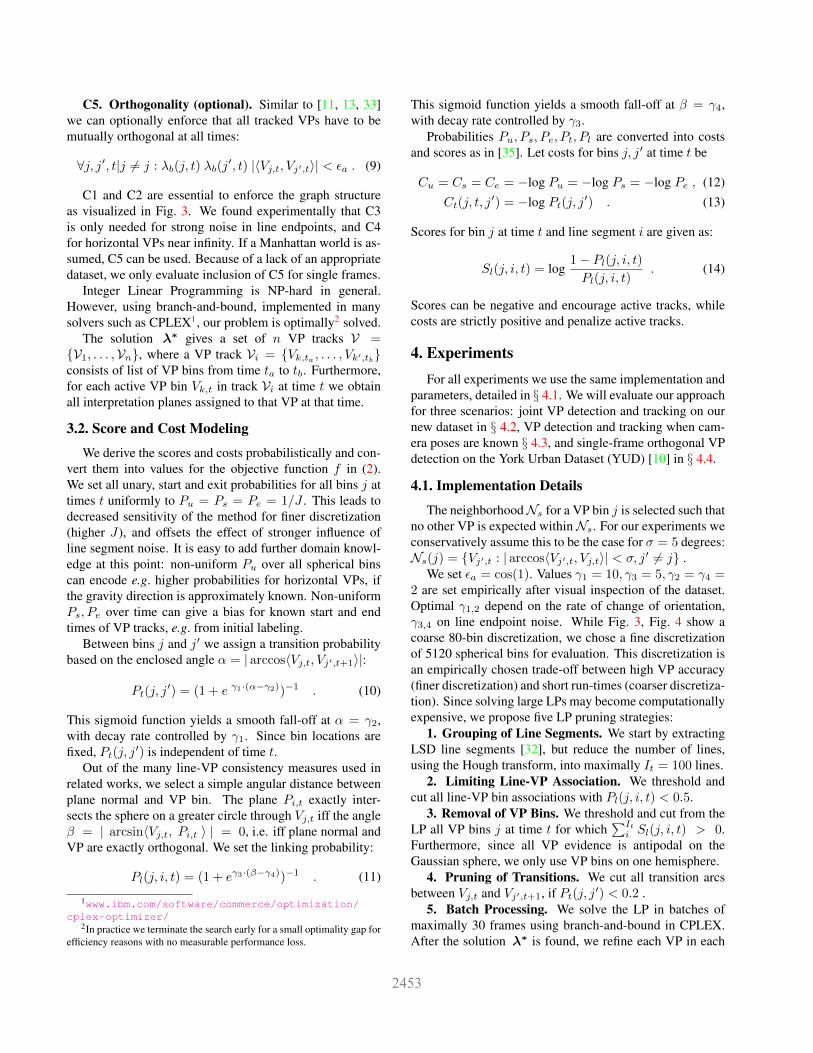
Figure 5: Cumulative MOTA and ID switches over 48 sequences for the Street-View evaluation in § 4.2. The result for the proposed method(LPMF) is colored in red. For MOTA our approach outperforms all baselines for 58 percent of the dataset, and is on par with the bestbaselines for the rest. For ID switches our method outperforms all baselines significantly over the whole dataset.

frame via least-squares optimization using Eq. (1). Batchesare greedily merged, as explained for our baselines in § 4.2.

Experimentally we found that these pruning steps do notchange the solution of the LP, but are helpful (esp. steps 1and 3) to keep the computation to a few seconds per frame.

4.2. Evaluation on the Street-View Dataset

Dataset: As the field lacks a dataset for the evaluationof joint VP detection and tracking we augmented a datasetfor video registration to SfM models [17] with our ownVP annotations. Multiple vanishing directions and identi-ties across frames were annotated semi-automatically in allframes, by using the known global camera pose and a super-vised interpretation plane clustering. We provide more in-formation about the annotation procedure in the supplemen-tary material. The annotations will be publicly available.The dataset consists of 48 sequences of 301 frames (at 10fps) of street-view video from van-mounted cameras, yield-ing a total of 14448 annotated frames with between zeroand three VPs. Due to the non-orthogonal street-layout, theManhattan world assumption is generally not valid for thisdataset. The videos are of varying difficulty for VP extrac-tion, and contain easy city scenes, as well as challengingscenes dominated by vegetation and street furniture.

Baselines: Since this is the first work for joint VP ex-traction and tracking, we construct our own baseline basedon [29]. We compare our method to two types of baselines.

The first baseline, LPSF (Linear Program, Single-Frame), corresponds to VP detection with our proposedmethod, where every frame is treated separately. Followingthe frame-wise VP extraction, we greedily grow VP tracks.Initially, the set of VP tracks is empty. For a new framewe merge VPs to existing VP tracks if the angular differ-ence is smaller then 5 degrees. The remaining VPs of this

new frame start new tracks. Finally, we remove VP tracksshorter than 3 frames. The second baseline, in several vari-ants, called TNO, for Tardif, Non-Orthogonal, correspond-ing to a recent single-frame VP extraction method [29],where we ignore the extension for orthogonal VPs. Sincethe VP detection sensitivity of [29] is strongly linked tothe image resolution, we downscale the image by factors{0.3, 0.4, 0.5, 0.6} to obtain better scores for this baseline.VP tracks are grown greedily as for LPSF. VP tracks shorterthan 3 frames are removed for the variants marked with f.

Results: We evaluate with two metrics commonlyused in tracking: multi-object tracking accuracy (MOTA,higher=better) [7], and ID switches (IDS,lower=better) [19].The result is visualized in Fig. 5. The VP matching thresh-old was set to an angle of 2 degrees. Our method is denotedas LPMF (Linear Program, Multi-Frame). For MOTA thebest baseline results are generally obtained with LPSF andTNO 0.4 f. The MOTA scores of TNO 0.4 f and TNO 0.5 fare very similar, but TNO 0.4 f has significantly fewer IDswitches. Stronger downscaling (≤ 0.3) leads to an in-crease in missed detections, and weaker downscaling (≥0.6) to many false positive detections. Removing short (< 3frames) VP tracks always increases MOTA and decreasesID switches. Stronger filtering leads to a loss in MOTA.

Greedy VP track linking in all baselines often fails, be-cause of the lack of temporal smoothness constraints in theVP detection. This leads to frequent loss and reinitializa-tion of VP tracks, yielding many ID switches. Our methodsignificantly outperforms all baselines in ID switches: in 75percent of the dataset no ground truth track is split. The bestbaseline on IDS, TNO 0.3 f, achieves this only for 41 percentof the dataset, with significantly worse MOTA. In MOTAour approach outperforms all baselines for 58 percent of thedataset, and is on par with the best baselines for MOTA> 0.

1 0.5 0 −0.5 −10

0.2

0.4

0.6

0.8

1

Cumulative MOTA score over all sequencesP

erc

en

t o

f seq

uen

ces w

ith

MO

TA

>=

X

MOTA score

LPMF

LPMF_kp

TNO_0.4_f

TNO_0.4_f_kp

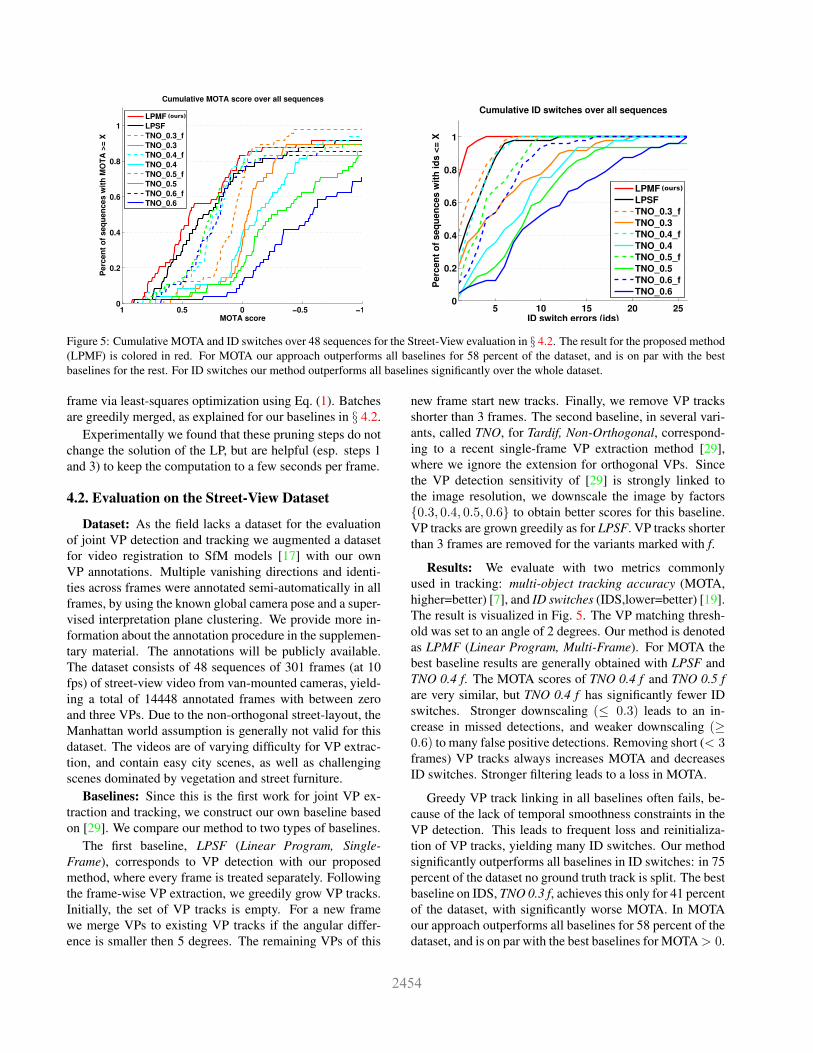
Figure 6: Cumulative MOTA for the evaluation in § 4.3. If poseknowledge is incorporated our method (LPMF kp) still outper-forms the best baseline (TNO 0.4 f kp) for most sequences.

For a MOTA threshold of 0.5, our method, and the two bestbaselines LPSF and TNO 0.4 f, have 42, 29 and 13 percent,respectively, of all sequences above this score. MOTA inall methods drops significantly for the most difficult 20 per-cent of all sequences. For all methods the strongest negativeinfluence on MOTA comes from missed VPs due to weakline support. In MOTP (multi-object tracking precision) allmethods offer very similar performance. We provide a de-tailed quantitative evaluation (MOTA, MOTP, IDS) for all48 videos in the supplementary material.

Our unoptimized single-core Matlab implementation(using CPLEX) requires 2.8 seconds per frame on averageon a Intel Core i7 CPU. One second is needed for prepro-cessing (line extraction, Hough grouping) and the rest forsolving the LP. The best baseline TNO 0.4 f runs for 0.7seconds per frame including line extraction. Recent relatedworks report runtimes from ’a few seconds’ [34] to halfa minute [30, 18] per frame for similar image resolutions,but without the need for finding temporal correspondences.The extra time required for our approach in comparison tothe TNO 0.4 f baseline is spent well on joint temporal dataassociation, since our method leads to significantly fewerfailure cases. This is demonstrated by two important exper-imental results: Firstly, our approach creates significantlyfewer false positive tracks, as reflected in the MOTA score.Secondly, our approach rarely splits a ground truth track: in75 percent of the dataset our approach does not have anyID switch, while this is only the case for 21 percent of allsequences for TNO 0.4 f. Low IDS is especially crucial forlong-term operations, in which continuous VP identity in-formation is needed and re-initializations are costly.

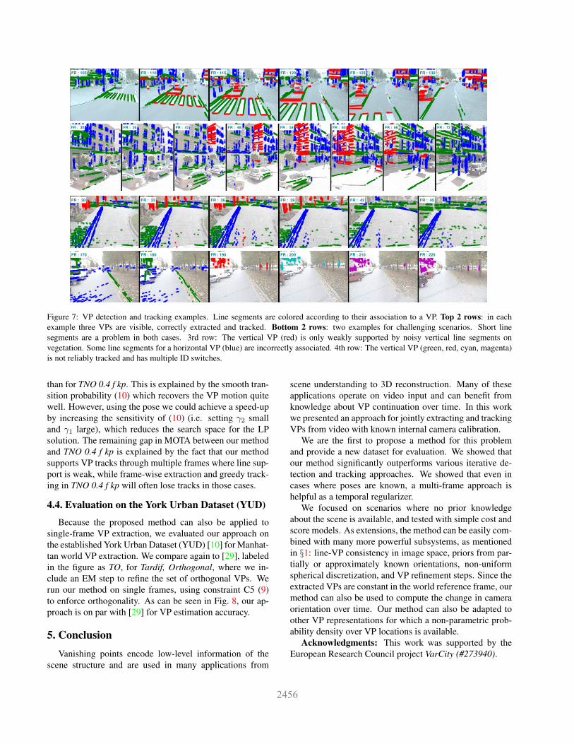
Some qualitative results are shown in Fig. 7. Lines whichwere associated to the same VP track are drawn in the samecolor. Examples for challenging scenes with failure cases

1 2 3 4 50

0.2

0.4

0.6

0.8

1

Allowed VP error in degrees

Per

cent

of V

Ps

with

err

or <

= X

Single Frame VP Accuracy

TO_1.0LPSF

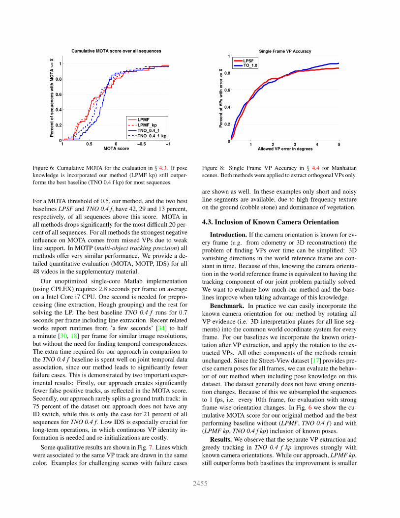
Figure 8: Single Frame VP Accuracy in § 4.4 for Manhattanscenes. Both methods were applied to extract orthogonal VPs only.

are shown as well. In these examples only short and noisyline segments are available, due to high-frequency textureon the ground (cobble stone) and dominance of vegetation.

4.3. Inclusion of Known Camera Orientation

Introduction. If the camera orientation is known for ev-ery frame (e.g. from odometry or 3D reconstruction) theproblem of finding VPs over time can be simplified: 3Dvanishing directions in the world reference frame are con-stant in time. Because of this, knowing the camera orienta-tion in the world reference frame is equivalent to having thetracking component of our joint problem partially solved.We want to evaluate how much our method and the base-lines improve when taking advantage of this knowledge.

Benchmark. In practice we can easily incorporate theknown camera orientation for our method by rotating allVP evidence (i.e. 3D interpretation planes for all line seg-ments) into the common world coordinate system for everyframe. For our baselines we incorporate the known orien-tation after VP extraction, and apply the rotation to the ex-tracted VPs. All other components of the methods remainunchanged. Since the Street-View dataset [17] provides pre-cise camera poses for all frames, we can evaluate the behav-ior of our method when including pose knowledge on thisdataset. The dataset generally does not have strong orienta-tion changes. Because of this we subsampled the sequencesto 1 fps, i.e. every 10th frame, for evaluation with strongframe-wise orientation changes. In Fig. 6 we show the cu-mulative MOTA score for our original method and the bestperforming baseline without (LPMF, TNO 0.4 f ) and with(LPMF kp, TNO 0.4 f kp) inclusion of known poses.

Results. We observe that the separate VP extraction andgreedy tracking in TNO 0.4 f kp improves strongly withknown camera orientations. While our approach, LPMF kp,still outperforms both baselines the improvement is smaller

FR : 105 FR : 110 FR : 115 FR : 120 FR : 125 FR : 130

FR : 30 FR : 36 FR : 42 FR : 48 FR : 54 FR : 60 FR : 66 FR : 72

FR : 30 FR : 33 FR : 36 FR : 39 FR : 42 FR : 45

FR : 170 FR : 180 FR : 190 FR : 200 FR : 210 FR : 220

Figure 7: VP detection and tracking examples. Line segments are colored according to their association to a VP. Top 2 rows: in eachexample three VPs are visible, correctly extracted and tracked. Bottom 2 rows: two examples for challenging scenarios. Short linesegments are a problem in both cases. 3rd row: The vertical VP (red) is only weakly supported by noisy vertical line segments onvegetation. Some line segments for a horizontal VP (blue) are incorrectly associated. 4th row: The vertical VP (green, red, cyan, magenta)is not reliably tracked and has multiple ID switches.

than for TNO 0.4 f kp. This is explained by the smooth tran-sition probability (10) which recovers the VP motion quitewell. However, using the pose we could achieve a speed-upby increasing the sensitivity of (10) (i.e. setting γ2 smalland γ1 large), which reduces the search space for the LPsolution. The remaining gap in MOTA between our methodand TNO 0.4 f kp is explained by the fact that our methodsupports VP tracks through multiple frames where line sup-port is weak, while frame-wise extraction and greedy track-ing in TNO 0.4 f kp will often lose tracks in those cases.

4.4. Evaluation on the York Urban Dataset (YUD)

Because the proposed method can also be applied tosingle-frame VP extraction, we evaluated our approach onthe established York Urban Dataset (YUD) [10] for Manhat-tan world VP extraction. We compare again to [29], labeledin the figure as TO, for Tardif, Orthogonal, where we in-clude an EM step to refine the set of orthogonal VPs. Werun our method on single frames, using constraint C5 (9)to enforce orthogonality. As can be seen in Fig. 8, our ap-proach is on par with [29] for VP estimation accuracy.

5. ConclusionVanishing points encode low-level information of the

scene structure and are used in many applications from

scene understanding to 3D reconstruction. Many of theseapplications operate on video input and can benefit fromknowledge about VP continuation over time. In this workwe presented an approach for jointly extracting and trackingVPs from video with known internal camera calibration.

We are the first to propose a method for this problemand provide a new dataset for evaluation. We showed thatour method significantly outperforms various iterative de-tection and tracking approaches. We showed that even incases where poses are known, a multi-frame approach ishelpful as a temporal regularizer.

We focused on scenarios where no prior knowledgeabout the scene is available, and tested with simple cost andscore models. As extensions, the method can be easily com-bined with many more powerful subsystems, as mentionedin §1: line-VP consistency in image space, priors from par-tially or approximately known orientations, non-uniformspherical discretization, and VP refinement steps. Since theextracted VPs are constant in the world reference frame, ourmethod can also be used to compute the change in cameraorientation over time. Our method can also be adapted toother VP representations for which a non-parametric prob-ability density over VP locations is available.

Acknowledgments: This work was supported by theEuropean Research Council project VarCity (#273940).

References[1] M. E. Antone and S. Teller. Automatic Recovery of Relative

Camera Rotations for Urban Scenes. In CVPR, 2000. 1, 2[2] M. Antunes and J. a. P. Barreto. A Global Approach for

the Detection of Vanishing Points and Mutually OrthogonalVanishing Directions. In CVPR. Ieee, 2013. 2, 4

[3] S. T. Barnard. Interpreting Perspective Images. ArtificialIntelligence, 1982. 2

[4] J.-C. Bazin, C. Demonceaux, P. Vasseur, and I. Kweon. Ro-tation estimation and vanishing point extraction by omnidi-rectional vision in urban environment. International Journalof Robotics Research, 31(1):63–81, 2012. 2

[5] J.-C. Bazin and M. Pollefeys. 3-line RANSAC for Orthogo-nal Vanishing Point Detection. IROS, 2012. 2

[6] J. Berclaz, F. Fleuret, E. Turetken, and P. Fua. Multiple Ob-ject Tracking using K-Shortest Paths Optimization. PAMI,2011. 1, 3

[7] K. Bernardin, A. Elbs, and R. Stiefelhagen. Multiple Ob-ject Tracking Performance Metrics and Evaluation in a SmartRoom Environment Performance Metrics for Multiple Ob-ject Tracking. EURASIP, 2008. 2, 6

[8] B. Caprile and V. Torre. Using Vanishing Points for CameraCalibration. IJCV, 1990. 2

[9] D. J. Crandall, A. Owens, N. Snavely, and D. P. Hutten-locher. SfM with MRFs: Discrete-Continuous Optimizationfor Large-Scale Structure from Motion. PAMI, 2012. 1

[10] P. Denis, J. H. Elder, and F. J. Estrada. Efficient Edge-Based Methods for Estimating Manhattan Frames in UrbanImagery. In ECCV, 2008. 2, 5, 8

[11] W. Elloumi, S. Treuillet, and R. Leconge. Tracking Orthogo-nal Vanishing Points in Video Sequences for a Reliable Cam-era Orientation in Manhattan World. In CISP, 2012. 1, 2, 5

[12] L. Grammatikopoulos, G. Karras, and E. Petsa. An Au-tomatic Approach for Camera Calibration from VanishingPoints. ISPRS Journal of Photogrammetry and Remote Sens-ing, 2007. 1, 2

[13] M. Hornacek and S. Maierhofer. Extracting Vanishing Pointsacross Multiple Views. In CVPR, 2011. 1, 2, 5

[14] C. Kim and R. Manduchi. Planar Structures from Line Cor-respondences in a Manhattan World. In ACCV, 2014. 1

[15] J. Kosecka and W. Zhang. Video Compass. In ECCV, 2002.1, 2

[16] T. Kroeger, D. Dai, R. Timofte, and L. Van Gool. Discoveryof Sets of Mutually Orthogonal Vanishing Points in Videos.In BMTT Workshop at WACV, 2015. 2

[17] T. Kroeger and L. Van Gool. Video Registration to SfMModels. In ECCV, 2014. 2, 6, 7

[18] J. Lezama, R. G. Von Gioi, G. Randall, and J.-m. Morel.Finding Vanishing Points via Point Alignments in Image Pri-mal and Dual Domains. In CVPR, 2014. 2, 7

[19] Y. Li, C. Huang, and R. Nevatia. Learning to associate:HybridBoosted multi-target tracker for crowded scene. InCVPR, 2009. 2, 6

[20] E. Lutton, H. Maıtre, and J. Lodez-Krahe. Contribution tothe Determination of Vanishing Points Using Hough Trans-form. PAMI, 1994. 2

[21] M. J. Magee and J. K. Aggarwal. Determining vanishingpoints from perspective images. Computer Vision, Graphics,and Image Processing, 1984. 2

[22] B. Micusik and H. Wildenauer. Minimal solution for uncali-brated absolute pose problem with a known vanishing point.In 3DVV, 2013. 1, 2

[23] P. Moghadam and J. F. Dong. Road Direction DetectionBased on Vanishing-Point Tracking. IROS, 2012. 1, 2

[24] L. Quan and R. Mohr. Determining perspective structures us-ing hierarchical Hough transform. Pattern Recognition Let-ters, 1989. 2

[25] C. Rasmussen. RoadCompass: following rural roads withvision + ladar using vanishing point tracking. AutonomousRobots, 2008. 1, 2

[26] C. Rother. A new approach to vanishing point detection inarchitectural environments. Image and Vision Computing,20, 2002. 2

[27] G. Schindler and F. Dellaert. Atlanta World: An Expecta-tion Maximization Framework for Simultaneous Low-levelEdge Grouping and Camera Calibration in Complex Man-made Environments. In CVPR, 2004. 2

[28] J. Straub, G. Rosman, O. Freifeld, J. J. Leonard, and J. W.Fisher III. A Mixture of Manhattan Frames : Beyond theManhattan World. In CVPR, 2014. 2

[29] J.-P. Tardif. Non-Iterative Approach for Fast and AccurateVanishing Point Detection. In ICCV, 2009. 2, 6, 8

[30] E. Tretyak, O. Barinova, P. Kohli, and V. Lempitsky. Ge-ometric Image Parsing in Man-Made Environments. IJCV,2012. 2, 7

[31] T. Tuytelaars, M. Proesmans, and L. V. Gool. The CascadedHough Transform as Support for Grouping and Finding Van-ishing Points and Lines. In AFPAC, 1997. 2

[32] R. G. von Gioi, J. Jakubowicz, J.-M. Morel, and G. Randall.LSD: a Line Segment Detector. IPOL, 2012. 5

[33] H. Wildenauer and A. Hanbury. Robust Camera Self-Calibration from Monocular Images of Manhattan Worlds.In CVPR, 2012. 1, 2, 5

[34] Y. Xu, S. Oh, and A. Hoogs. A Minimum Error VanishingPoint Detection Approach for Uncalibrated Monocular Im-ages of Man-made Environments. In CVPR, 2013. 2, 7

[35] L. Zhang, Y. Li, and R. Nevatia. Global Data Associationfor Multi-Object Tracking Using Network Flows. In CVPR,2008. 1, 3, 4, 5