Embed Size (px)
Citation preview
Entropy viscosity
Jean-Luc Guermond & Bojan Popov
Department of MathematicsTexas A&M University
Sparsity and ComputationJune 7-11, 2010
University of Bonn
Jean-Luc Guermond & Bojan Popov Entropy viscosity
Acknowledgments
Collaborator: Andrea Bonito, Texas A&MCollaborator: Richard Pasquetti, Univ. Nice
Support: NSF (DMS 0510650, 0811041), LLNL, KAUST, AFSOR
Jean-Luc Guermond & Bojan Popov Entropy viscosity
Outline
1 INTRODUCTION
2 LINEAR TRANSPORT EQUATION
3 NONLINEAR SCALAR CONSERVATION
4 COMPRESSIBLE EULER EQUATIONS
Jean-Luc Guermond & Bojan Popov Entropy viscosity
Outline
1 INTRODUCTION
2 LINEAR TRANSPORT EQUATION
3 NONLINEAR SCALAR CONSERVATION
4 COMPRESSIBLE EULER EQUATIONS
Jean-Luc Guermond & Bojan Popov Entropy viscosity
Outline
1 INTRODUCTION
2 LINEAR TRANSPORT EQUATION
3 NONLINEAR SCALAR CONSERVATION
4 COMPRESSIBLE EULER EQUATIONS
Jean-Luc Guermond & Bojan Popov Entropy viscosity
Outline
1 INTRODUCTION
2 LINEAR TRANSPORT EQUATION
3 NONLINEAR SCALAR CONSERVATION
4 COMPRESSIBLE EULER EQUATIONS
Jean-Luc Guermond & Bojan Popov Entropy viscosity
INTRODUCTIONLINEAR TRANSPORT EQUATION
NONLINEAR SCALAR CONSERVATIONCOMPRESSIBLE EULER EQUATIONS
Why L1 for PDEs?Why L1 is not so good for PDEs?Can L1 help anyway?
NONLINEAR SCALAR CONSERVATION EQUATIONS
Introduction
1 INTRODUCTION2 LINEAR TRANSPORT EQUATION3 NONLINEAR SCALAR CONSERVATION4 COMPRESSIBLE EULER EQUATIONS
Jean-Luc Guermond & Bojan Popov Entropy viscosity
INTRODUCTIONLINEAR TRANSPORT EQUATION
NONLINEAR SCALAR CONSERVATIONCOMPRESSIBLE EULER EQUATIONS
Why L1 for PDEs?Why L1 is not so good for PDEs?Can L1 help anyway?
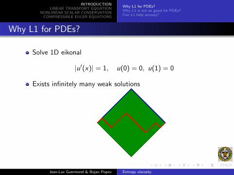
Why L1 for PDEs?
Solve 1D eikonal
|u′(x)| = 1, u(0) = 0, u(1) = 0
Exists infinitely many weak solutions
Jean-Luc Guermond & Bojan Popov Entropy viscosity
INTRODUCTIONLINEAR TRANSPORT EQUATION
NONLINEAR SCALAR CONSERVATIONCOMPRESSIBLE EULER EQUATIONS
Why L1 for PDEs?Why L1 is not so good for PDEs?Can L1 help anyway?
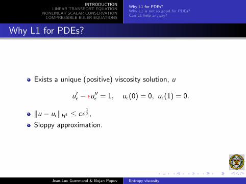
Why L1 for PDEs?
Exists a unique (positive) viscosity solution, u
u′ε − εu′′ε = 1, uε(0) = 0, uε(1) = 0.
‖u − uε‖H1 ≤ cε12 ,
Sloppy approximation.
Jean-Luc Guermond & Bojan Popov Entropy viscosity
INTRODUCTIONLINEAR TRANSPORT EQUATION
NONLINEAR SCALAR CONSERVATIONCOMPRESSIBLE EULER EQUATIONS
Why L1 for PDEs?Why L1 is not so good for PDEs?Can L1 help anyway?
Why L1 for PDEs?
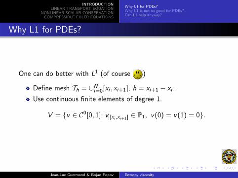
One can do better with L1 (of course )
Define mesh Th = ∪Ni=0[xi , xi+1], h = xi+1 − xi .
Use continuous finite elements of degree 1.
V = v ∈ C0[0, 1]; v|[xi ,xi+1] ∈ P1, v(0) = v(1) = 0.
Jean-Luc Guermond & Bojan Popov Entropy viscosity
INTRODUCTIONLINEAR TRANSPORT EQUATION
NONLINEAR SCALAR CONSERVATIONCOMPRESSIBLE EULER EQUATIONS
Why L1 for PDEs?Why L1 is not so good for PDEs?Can L1 help anyway?
Why L1 for PDEs?
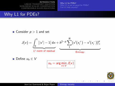
Consider p > 1 and set
J(v) =
∫ 1
0
∣∣|v ′| − 1∣∣ dx︸ ︷︷ ︸
L1-norm of residual
+ h2−pN∑1
(v ′(x+i )− v ′(x−i ))p
+︸ ︷︷ ︸Entropy
Define uh ∈ Vuh = arg min
v∈VJ(v)
Jean-Luc Guermond & Bojan Popov Entropy viscosity
INTRODUCTIONLINEAR TRANSPORT EQUATION
NONLINEAR SCALAR CONSERVATIONCOMPRESSIBLE EULER EQUATIONS
Why L1 for PDEs?Why L1 is not so good for PDEs?Can L1 help anyway?
Why L1 for PDEs?
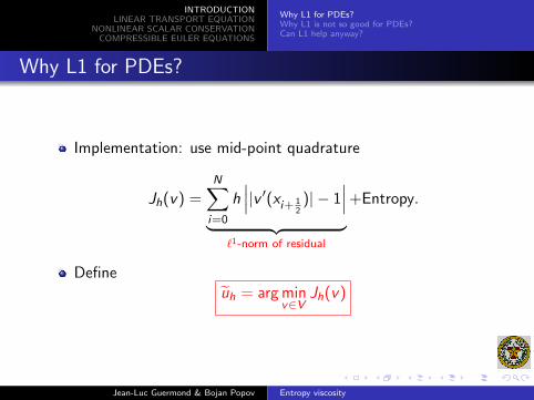
Implementation: use mid-point quadrature
Jh(v) =N∑
i=0
h∣∣∣|v ′(xi+ 1
2)| − 1
∣∣∣︸ ︷︷ ︸`1-norm of residual
+Entropy.
Defineuh = arg min
v∈VJh(v)
Jean-Luc Guermond & Bojan Popov Entropy viscosity
INTRODUCTIONLINEAR TRANSPORT EQUATION
NONLINEAR SCALAR CONSERVATIONCOMPRESSIBLE EULER EQUATIONS
Why L1 for PDEs?Why L1 is not so good for PDEs?Can L1 help anyway?
Why L1 for PDEs?
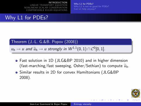
Theorem (J.-L. G.&B. Popov (2008))
uh → u and uh → u strongly in W 1,1(0, 1) ∩ C0[0, 1].
Fast solution in 1D (JLG&BP 2010) and in higher dimension(fast-marching/fast sweeping, Osher/Sethian) to compute uh.
Similar results in 2D for convex Hamiltonians (JLG&BP2008).
Jean-Luc Guermond & Bojan Popov Entropy viscosity
INTRODUCTIONLINEAR TRANSPORT EQUATION
NONLINEAR SCALAR CONSERVATIONCOMPRESSIBLE EULER EQUATIONS
Why L1 for PDEs?Why L1 is not so good for PDEs?Can L1 help anyway?
Why L1 is not so good for PDEs?
Generalization to conservation laws? (yet to be done).
L1-minimization cannot compete (yet) with explicit schemesfor time-dependent conservation laws.
Jean-Luc Guermond & Bojan Popov Entropy viscosity
INTRODUCTIONLINEAR TRANSPORT EQUATION
NONLINEAR SCALAR CONSERVATIONCOMPRESSIBLE EULER EQUATIONS
Why L1 for PDEs?Why L1 is not so good for PDEs?Can L1 help anyway?
Why L1 is not so good for PDEs?
What is the problem with current time-stepping algorithms?1 Limiters2 Tensor product of 1D algorithms3 Use Cartesian grids
Jean-Luc Guermond & Bojan Popov Entropy viscosity
INTRODUCTIONLINEAR TRANSPORT EQUATION
NONLINEAR SCALAR CONSERVATIONCOMPRESSIBLE EULER EQUATIONS
Why L1 for PDEs?Why L1 is not so good for PDEs?Can L1 help anyway?
Can L1 help anyway?
Some provable properties of minimizer uh
(JLG&BP 2008, 2009, 2010). Minimizer uh is such that:
Residual is sparse:
|u′h(xi+ 12)| − 1 = 0, ∀i such that
1
26∈ [xi , xi+1].
Entropy makes it so that graph of u′h(x) is concave down in[xi , xi+1] 3 1
2 .
Jean-Luc Guermond & Bojan Popov Entropy viscosity
INTRODUCTIONLINEAR TRANSPORT EQUATION
NONLINEAR SCALAR CONSERVATIONCOMPRESSIBLE EULER EQUATIONS
Why L1 for PDEs?Why L1 is not so good for PDEs?Can L1 help anyway?
Can L1 help anyway?
Conclusion:
Residual is sparse: PDE solved almost everywhere. Entropydoes not play role in those cells.
Entropy plays a key role in cell where PDE is not solved.
Jean-Luc Guermond & Bojan Popov Entropy viscosity
INTRODUCTIONLINEAR TRANSPORT EQUATION
NONLINEAR SCALAR CONSERVATIONCOMPRESSIBLE EULER EQUATIONS
Why L1 for PDEs?Why L1 is not so good for PDEs?Can L1 help anyway?
Can L1 help anyway?
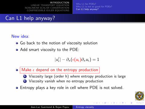
New idea:
Go back to the notion of viscosity solution
Add smart viscosity to the PDE:
|u′ε| − ∂x(ε(uε)∂xuε) = 1
Make ε depend on the entropy production
1 Viscosity large (order h) where entropy production is large2 Viscosity vanish when no entropy production
Entropy plays a key role in cell where PDE is not solved.
Jean-Luc Guermond & Bojan Popov Entropy viscosity
INTRODUCTIONLINEAR TRANSPORT EQUATION
NONLINEAR SCALAR CONSERVATIONCOMPRESSIBLE EULER EQUATIONS
Linear transportThe ideaThe algorithmA little bit of theoryNumerical tests
NONLINEAR SCALAR CONSERVATION EQUATIONS
Transport,mixing
1 INTRODUCTION2 LINEAR TRANSPORT EQUATION3 NONLINEAR SCALAR CONSERVATION4 COMPRESSIBLE EULER EQUATIONS
Jean-Luc Guermond & Bojan Popov Entropy viscosity
INTRODUCTIONLINEAR TRANSPORT EQUATION
NONLINEAR SCALAR CONSERVATIONCOMPRESSIBLE EULER EQUATIONS
Linear transportThe ideaThe algorithmA little bit of theoryNumerical tests
The PDE
Solve the transport equation
∂tu + β·∇u = 0, u|t=0 = u0, +BCs
Use standard discretizations (ex: continuous finite elements)
Deviate as little possible from Galerkin.
Jean-Luc Guermond & Bojan Popov Entropy viscosity
INTRODUCTIONLINEAR TRANSPORT EQUATION
NONLINEAR SCALAR CONSERVATIONCOMPRESSIBLE EULER EQUATIONS
Linear transportThe ideaThe algorithmA little bit of theoryNumerical tests
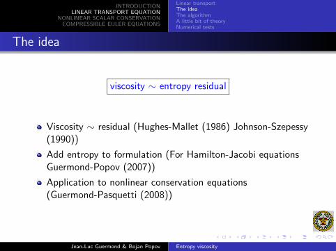
The idea
viscosity ∼ entropy residual
Viscosity ∼ residual (Hughes-Mallet (1986) Johnson-Szepessy(1990))
Add entropy to formulation (For Hamilton-Jacobi equationsGuermond-Popov (2007))
Application to nonlinear conservation equations(Guermond-Pasquetti (2008))
Jean-Luc Guermond & Bojan Popov Entropy viscosity
INTRODUCTIONLINEAR TRANSPORT EQUATION
NONLINEAR SCALAR CONSERVATIONCOMPRESSIBLE EULER EQUATIONS
Linear transportThe ideaThe algorithmA little bit of theoryNumerical tests
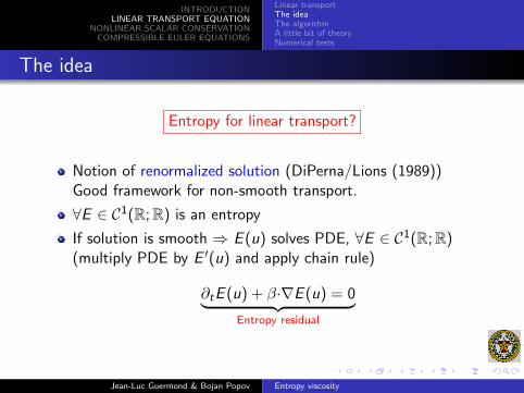
The idea
Entropy for linear transport?
Notion of renormalized solution (DiPerna/Lions (1989))Good framework for non-smooth transport.
∀E ∈ C1(R; R) is an entropy
If solution is smooth ⇒ E (u) solves PDE, ∀E ∈ C1(R; R)(multiply PDE by E ′(u) and apply chain rule)
∂tE (u) + β·∇E (u) = 0︸ ︷︷ ︸Entropy residual
Jean-Luc Guermond & Bojan Popov Entropy viscosity
INTRODUCTIONLINEAR TRANSPORT EQUATION
NONLINEAR SCALAR CONSERVATIONCOMPRESSIBLE EULER EQUATIONS
Linear transportThe ideaThe algorithmA little bit of theoryNumerical tests
The idea
Key idea 1:
Use entropy residual to construct viscosity
Jean-Luc Guermond & Bojan Popov Entropy viscosity
INTRODUCTIONLINEAR TRANSPORT EQUATION
NONLINEAR SCALAR CONSERVATIONCOMPRESSIBLE EULER EQUATIONS
Linear transportThe ideaThe algorithmA little bit of theoryNumerical tests
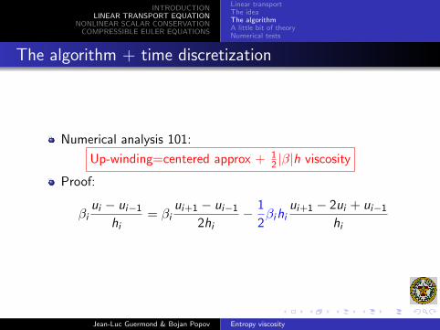
The algorithm + time discretization
Numerical analysis 101:
Up-winding=centered approx + 12 |β|h viscosity
Proof:
βiui − ui−1
hi= βi
ui+1 − ui−1
2hi− 1
2βihi
ui+1 − 2ui + ui−1
hi
Jean-Luc Guermond & Bojan Popov Entropy viscosity
INTRODUCTIONLINEAR TRANSPORT EQUATION
NONLINEAR SCALAR CONSERVATIONCOMPRESSIBLE EULER EQUATIONS
Linear transportThe ideaThe algorithmA little bit of theoryNumerical tests
The algorithm + time discretization
Key idea 2:
Entropy viscosity should not exceed 12|β|h
Jean-Luc Guermond & Bojan Popov Entropy viscosity
INTRODUCTIONLINEAR TRANSPORT EQUATION
NONLINEAR SCALAR CONSERVATIONCOMPRESSIBLE EULER EQUATIONS
Linear transportThe ideaThe algorithmA little bit of theoryNumerical tests
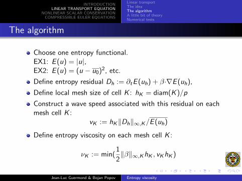
The algorithm
Choose one entropy functional.EX1: E (u) = |u|,EX2: E (u) = (u − u0)2, etc.
Define entropy residual Dh := ∂tE (uh) + β·∇E (uh),
Define local mesh size of cell K : hK = diam(K )/p
Construct a wave speed associated with this residual on eachmesh cell K :
vK := hK‖Dh‖∞,K/E (uh)
Define entropy viscosity on each mesh cell K :
νK := min(1
2‖β‖∞,K hK , vK hK )
Jean-Luc Guermond & Bojan Popov Entropy viscosity
INTRODUCTIONLINEAR TRANSPORT EQUATION
NONLINEAR SCALAR CONSERVATIONCOMPRESSIBLE EULER EQUATIONS
Linear transportThe ideaThe algorithmA little bit of theoryNumerical tests
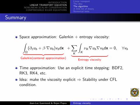
Summary
Space approximation: Galerkin + entropy viscosity:∫Ω
(∂tuh + β·∇uh)vhdx︸ ︷︷ ︸Galerkin(centered approximation)
+∑K
∫KνK∇uh∇vhdx︸ ︷︷ ︸
Entropy viscosity
= 0, ∀vh
Time approximation: Use an explicit time stepping: BDF2,RK3, RK4, etc.
Idea: make the viscosity explicit ⇒ Stability under CFLcondition.
Jean-Luc Guermond & Bojan Popov Entropy viscosity
INTRODUCTIONLINEAR TRANSPORT EQUATION
NONLINEAR SCALAR CONSERVATIONCOMPRESSIBLE EULER EQUATIONS
Linear transportThe ideaThe algorithmA little bit of theoryNumerical tests
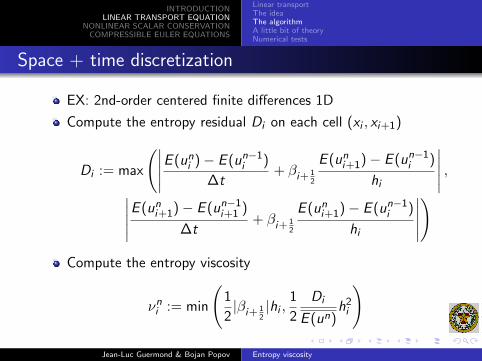
Space + time discretization
EX: 2nd-order centered finite differences 1D
Compute the entropy residual Di on each cell (xi , xi+1)
Di := max
(∣∣∣∣∣E (uni )− E (un−1
i )
∆t+ βi+ 1
2
E (uni+1)− E (un−1
i )
hi
∣∣∣∣∣ ,∣∣∣∣∣E (uni+1)− E (un−1
i+1 )
∆t+ βi+ 1
2
E (uni+1)− E (un−1
i )
hi
∣∣∣∣∣)
Compute the entropy viscosity
νni := min
(1
2|βi+ 1
2|hi ,
1
2
Di
E (un)h2i
)
Jean-Luc Guermond & Bojan Popov Entropy viscosity
INTRODUCTIONLINEAR TRANSPORT EQUATION
NONLINEAR SCALAR CONSERVATIONCOMPRESSIBLE EULER EQUATIONS
Linear transportThe ideaThe algorithmA little bit of theoryNumerical tests
Space + time discretization
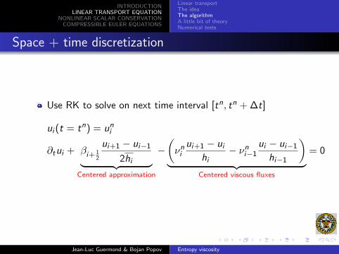
Use RK to solve on next time interval [tn, tn + ∆t]
ui (t = tn) = uni
∂tui + βi+ 12
ui+1 − ui−1
2hi︸ ︷︷ ︸Centered approximation
−(νni
ui+1 − ui
hi− νn
i−1
ui − ui−1
hi−1
)︸ ︷︷ ︸
Centered viscous fluxes
= 0
Jean-Luc Guermond & Bojan Popov Entropy viscosity
INTRODUCTIONLINEAR TRANSPORT EQUATION
NONLINEAR SCALAR CONSERVATIONCOMPRESSIBLE EULER EQUATIONS
Linear transportThe ideaThe algorithmA little bit of theoryNumerical tests
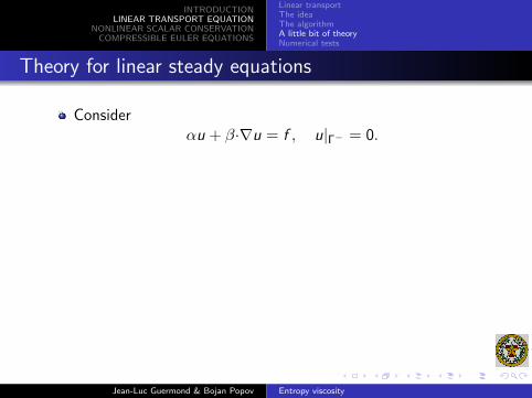
Theory for linear steady equations
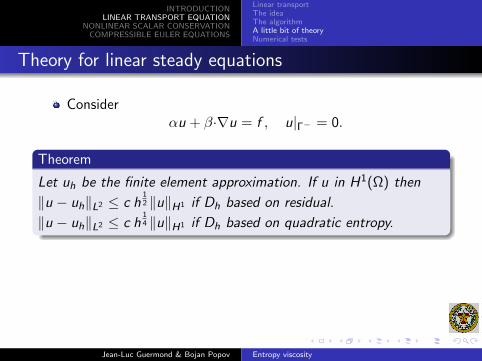
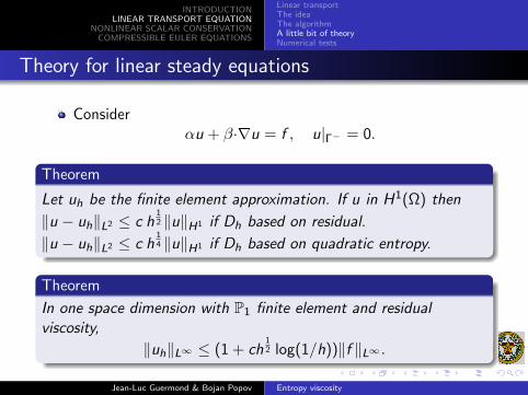
Considerαu + β·∇u = f , u|Γ− = 0.
Theorem
Let uh be the finite element approximation. If u in H1(Ω) then
‖u − uh‖L2 ≤ c h12 ‖u‖H1 if Dh based on residual.
‖u − uh‖L2 ≤ c h14 ‖u‖H1 if Dh based on quadratic entropy.
Theorem
In one space dimension with P1 finite element and residualviscosity,
‖uh‖L∞ ≤ (1 + ch12 log(1/h))‖f ‖L∞ .
Jean-Luc Guermond & Bojan Popov Entropy viscosity
INTRODUCTIONLINEAR TRANSPORT EQUATION
NONLINEAR SCALAR CONSERVATIONCOMPRESSIBLE EULER EQUATIONS
Linear transportThe ideaThe algorithmA little bit of theoryNumerical tests
Theory for linear steady equations
Considerαu + β·∇u = f , u|Γ− = 0.
Theorem
Let uh be the finite element approximation. If u in H1(Ω) then
‖u − uh‖L2 ≤ c h12 ‖u‖H1 if Dh based on residual.
‖u − uh‖L2 ≤ c h14 ‖u‖H1 if Dh based on quadratic entropy.
Theorem
In one space dimension with P1 finite element and residualviscosity,
‖uh‖L∞ ≤ (1 + ch12 log(1/h))‖f ‖L∞ .
Jean-Luc Guermond & Bojan Popov Entropy viscosity

INTRODUCTIONLINEAR TRANSPORT EQUATION
NONLINEAR SCALAR CONSERVATIONCOMPRESSIBLE EULER EQUATIONS
Linear transportThe ideaThe algorithmA little bit of theoryNumerical tests
Theory for linear steady equations
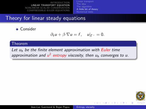
Consider∂tu + β·∇u = f , u|Γ− = 0.
Theorem
Let uh be the finite element approximation with Euler timeapproximation and u2 entropy viscosity, then uh converges to u.
Theorem
Let uh be the P1 finite element approximation with RK2 timeapproximation and residual viscosity, then uh converges to u.
Conjecture
The results should hold for nonlinear scalar conservation laws withconvex, Lipschitz flux.
Jean-Luc Guermond & Bojan Popov Entropy viscosity
INTRODUCTIONLINEAR TRANSPORT EQUATION
NONLINEAR SCALAR CONSERVATIONCOMPRESSIBLE EULER EQUATIONS
Linear transportThe ideaThe algorithmA little bit of theoryNumerical tests
Theory for linear steady equations
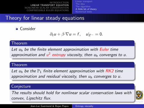
Consider∂tu + β·∇u = f , u|Γ− = 0.
Theorem
Let uh be the finite element approximation with Euler timeapproximation and u2 entropy viscosity, then uh converges to u.
Theorem
Let uh be the P1 finite element approximation with RK2 timeapproximation and residual viscosity, then uh converges to u.
Conjecture
The results should hold for nonlinear scalar conservation laws withconvex, Lipschitz flux.
Jean-Luc Guermond & Bojan Popov Entropy viscosity
INTRODUCTIONLINEAR TRANSPORT EQUATION
NONLINEAR SCALAR CONSERVATIONCOMPRESSIBLE EULER EQUATIONS
Linear transportThe ideaThe algorithmA little bit of theoryNumerical tests
Theory for linear steady equations
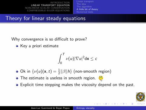
Why convergence is so difficult to prove?
Key a priori estimate∫ T
0ν(u)|∇u|2dx ≤ c
Ok in ν(u)(x, t) = 12‖β‖h (non-smooth region)
The estimate is useless in smooth region.
Explicit time stepping makes the viscosity depend on the past.
Jean-Luc Guermond & Bojan Popov Entropy viscosity
INTRODUCTIONLINEAR TRANSPORT EQUATION
NONLINEAR SCALAR CONSERVATIONCOMPRESSIBLE EULER EQUATIONS
Linear transportThe ideaThe algorithmA little bit of theoryNumerical tests
1D Numerical tests, BV solution
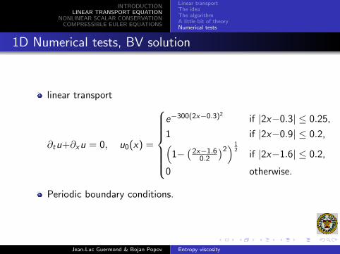
linear transport
∂tu+∂xu = 0, u0(x) =
e−300(2x−0.3)2if |2x−0.3| ≤ 0.25,
1 if |2x−0.9| ≤ 0.2,(1−(
2x−1.60.2
)2) 1
2if |2x−1.6| ≤ 0.2,
0 otherwise.
Periodic boundary conditions.
Jean-Luc Guermond & Bojan Popov Entropy viscosity
INTRODUCTIONLINEAR TRANSPORT EQUATION
NONLINEAR SCALAR CONSERVATIONCOMPRESSIBLE EULER EQUATIONS
Linear transportThe ideaThe algorithmA little bit of theoryNumerical tests
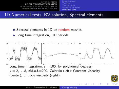
1D Numerical tests, BV solution, Spectral elements
Spectral elements in 1D on random meshes.
Long time integration, 100 periods.
Long time integration, t = 100, for polynomial degreesk = 2, . . . 8, #d.o.f.=200. Galerkin (left); Constant viscosity(center); Entropy viscosity (right).
Jean-Luc Guermond & Bojan Popov Entropy viscosity
INTRODUCTIONLINEAR TRANSPORT EQUATION
NONLINEAR SCALAR CONSERVATIONCOMPRESSIBLE EULER EQUATIONS
Linear transportThe ideaThe algorithmA little bit of theoryNumerical tests
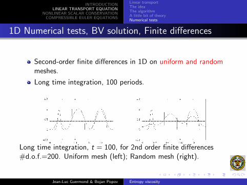
1D Numerical tests, BV solution, Finite differences
Second-order finite differences in 1D on uniform and randommeshes.
Long time integration, 100 periods.
Long time integration, t = 100, for 2nd order finite differences#d.o.f.=200. Uniform mesh (left); Random mesh (right).
Jean-Luc Guermond & Bojan Popov Entropy viscosity
INTRODUCTIONLINEAR TRANSPORT EQUATION
NONLINEAR SCALAR CONSERVATIONCOMPRESSIBLE EULER EQUATIONS
Linear transportThe ideaThe algorithmA little bit of theoryNumerical tests
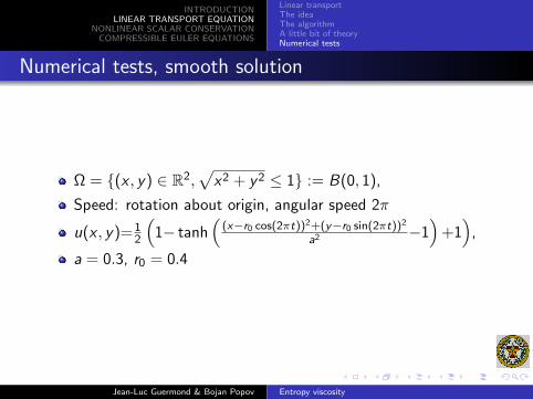
Numerical tests, smooth solution
Ω = (x , y) ∈ R2,√
x2 + y 2 ≤ 1 := B(0, 1),
Speed: rotation about origin, angular speed 2π
u(x , y)= 12
(1− tanh
((x−r0 cos(2πt))2+(y−r0 sin(2πt))2
a2 −1)
+1)
,
a = 0.3, r0 = 0.4
Jean-Luc Guermond & Bojan Popov Entropy viscosity
INTRODUCTIONLINEAR TRANSPORT EQUATION
NONLINEAR SCALAR CONSERVATIONCOMPRESSIBLE EULER EQUATIONS
Linear transportThe ideaThe algorithmA little bit of theoryNumerical tests
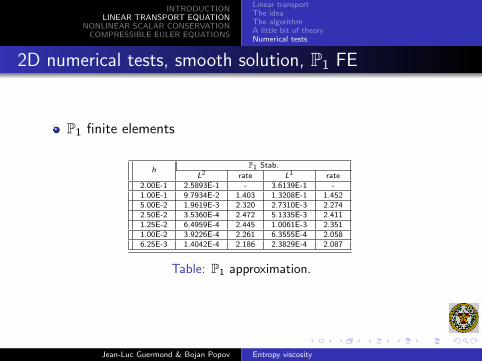
2D numerical tests, smooth solution, P1 FE
P1 finite elements
hP1 Stab.
L2 rate L1 rate2.00E-1 2.5893E-1 - 3.6139E-1 -1.00E-1 9.7934E-2 1.403 1.3208E-1 1.4525.00E-2 1.9619E-3 2.320 2.7310E-3 2.2742.50E-2 3.5360E-4 2.472 5.1335E-3 2.4111.25E-2 6.4959E-4 2.445 1.0061E-3 2.3511.00E-2 3.9226E-4 2.261 6.3555E-4 2.0586.25E-3 1.4042E-4 2.186 2.3829E-4 2.087
Table: P1 approximation.
Jean-Luc Guermond & Bojan Popov Entropy viscosity

INTRODUCTIONLINEAR TRANSPORT EQUATION
NONLINEAR SCALAR CONSERVATIONCOMPRESSIBLE EULER EQUATIONS
Linear transportThe ideaThe algorithmA little bit of theoryNumerical tests
2D numerical tests, smooth solution, spectral elements
1e-12
1e-11
1e-10
1e-09
1e-08
1e-07
1e-06
1e-05
1e-04
0.001
0.01
0.1
0.01 0.1 1
Err
or in
L1
norm
Element size h
N=2N=3N=4N=6
N=12 1e-12
1e-11
1e-10
1e-09
1e-08
1e-07
1e-06
1e-05
1e-04
0.001
0.01
0.1
0.01 0.1 1
Err
or in
L2
norm
Element size h
N=2N=3N=4N=6
N=12
Linear transport problem with smooth initial condition. Errors inL1 (at left) and L2 (at right) norms vs h for N = 2, 4, 6, 8, 12.
Jean-Luc Guermond & Bojan Popov Entropy viscosity
INTRODUCTIONLINEAR TRANSPORT EQUATION
NONLINEAR SCALAR CONSERVATIONCOMPRESSIBLE EULER EQUATIONS
Linear transportThe ideaThe algorithmA little bit of theoryNumerical tests
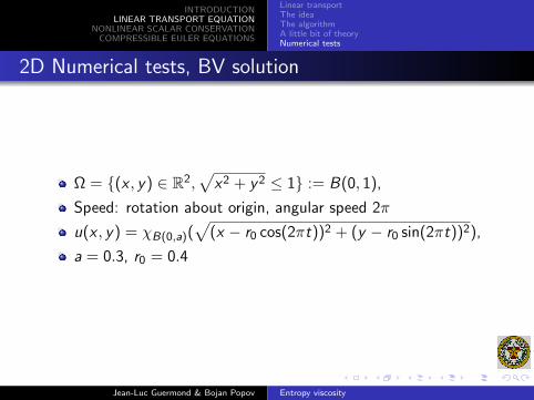
2D Numerical tests, BV solution
Ω = (x , y) ∈ R2,√
x2 + y 2 ≤ 1 := B(0, 1),
Speed: rotation about origin, angular speed 2π
u(x , y) = χB(0,a)(√
(x − r0 cos(2πt))2 + (y − r0 sin(2πt))2),
a = 0.3, r0 = 0.4
Jean-Luc Guermond & Bojan Popov Entropy viscosity
INTRODUCTIONLINEAR TRANSPORT EQUATION
NONLINEAR SCALAR CONSERVATIONCOMPRESSIBLE EULER EQUATIONS
Linear transportThe ideaThe algorithmA little bit of theoryNumerical tests
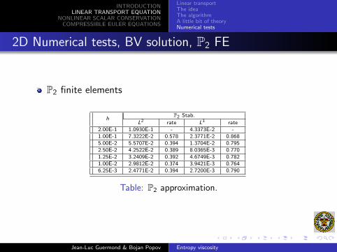
2D Numerical tests, BV solution, P2 FE
P2 finite elements
hP2 Stab.
L2 rate L1 rate2.00E-1 1.0930E-1 - 4.3373E-2 -1.00E-1 7.3222E-2 0.578 2.3771E-2 0.8685.00E-2 5.5707E-2 0.394 1.3704E-2 0.7952.50E-2 4.2522E-2 0.389 8.0365E-3 0.7701.25E-2 3.2409E-2 0.392 4.6749E-3 0.7821.00E-2 2.9812E-2 0.374 3.9421E-3 0.7646.25E-3 2.4771E-2 0.394 2.7200E-3 0.790
Table: P2 approximation.
Jean-Luc Guermond & Bojan Popov Entropy viscosity

INTRODUCTIONLINEAR TRANSPORT EQUATION
NONLINEAR SCALAR CONSERVATIONCOMPRESSIBLE EULER EQUATIONS
Nonlinear scalar conservation lawsConvergence tests, 2D Burgers, P1/P2 FEBuckley Leverett, FEKurganov, Petrova, Popov problem, FE
NONLINEAR SCALAR CONSERVATION EQUATIONS
JohannesMartinusBurgers
1 INTRODUCTION2 LINEAR TRANSPORT EQUATION3 NONLINEAR SCALAR CONSERVATION4 COMPRESSIBLE EULER EQUATIONS
Jean-Luc Guermond & Bojan Popov Entropy viscosity
INTRODUCTIONLINEAR TRANSPORT EQUATION
NONLINEAR SCALAR CONSERVATIONCOMPRESSIBLE EULER EQUATIONS
Nonlinear scalar conservation lawsConvergence tests, 2D Burgers, P1/P2 FEBuckley Leverett, FEKurganov, Petrova, Popov problem, FE
2D Nonlinear scalar conservation laws
Solve
∂tu + ∂x f (u) + ∂y g(u) = 0 u|t=0 = u0, +BCs.
The unique entropy solution satisfies
∂tE (u) + ∂xF (u) + ∂y G (u) ≤ 0
for all entropy pair E (u), F (u) =∫
E ′(u)f ′(u)du,G (u) =
∫E ′(u)g ′(u)du
Jean-Luc Guermond & Bojan Popov Entropy viscosity
INTRODUCTIONLINEAR TRANSPORT EQUATION
NONLINEAR SCALAR CONSERVATIONCOMPRESSIBLE EULER EQUATIONS
Nonlinear scalar conservation lawsConvergence tests, 2D Burgers, P1/P2 FEBuckley Leverett, FEKurganov, Petrova, Popov problem, FE
2D scalar nonlinear conservation laws
Choose one entropy E (u)
Define entropy residual, Dh(u) := ∂tE (u) + ∂xF (u) + ∂y G (u)
Define local mesh size of cell K : hK = diam(K )/p
Construct a speed associated with residual on each cell K :
vK := hK‖Dh‖∞,K/E (uh)
Compute maximum local wave speed:βK = ‖
√f ′(u)2 + g ′(u)2‖∞,K
Define entropy viscosity on each mesh cell K :
νK := hK min(1
2βK , vK )
Jean-Luc Guermond & Bojan Popov Entropy viscosity
INTRODUCTIONLINEAR TRANSPORT EQUATION
NONLINEAR SCALAR CONSERVATIONCOMPRESSIBLE EULER EQUATIONS
Nonlinear scalar conservation lawsConvergence tests, 2D Burgers, P1/P2 FEBuckley Leverett, FEKurganov, Petrova, Popov problem, FE
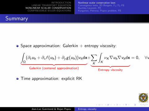
Summary
Space approximation: Galerkin + entropy viscosity:∫Ω
(∂tuh + ∂x f (uh) + ∂y g(uh))vhdx︸ ︷︷ ︸Galerkin (centered approximation)
+∑K
∫KνK∇uh∇vhdx︸ ︷︷ ︸
Entropy viscosity
= 0, ∀vh
Time approximation: explicit RK
Jean-Luc Guermond & Bojan Popov Entropy viscosity
INTRODUCTIONLINEAR TRANSPORT EQUATION
NONLINEAR SCALAR CONSERVATIONCOMPRESSIBLE EULER EQUATIONS
Nonlinear scalar conservation lawsConvergence tests, 2D Burgers, P1/P2 FEBuckley Leverett, FEKurganov, Petrova, Popov problem, FE
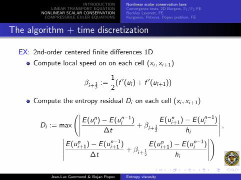
The algorithm + time discretization
EX: 2nd-order centered finite differences 1D
Compute local speed on on each cell (xi , xi+1)
βi+ 12
:=1
2(f ′(ui ) + f ′(ui+1))
Compute the entropy residual Di on each cell (xi , xi+1)
Di := max
(∣∣∣∣∣E (uni )− E (un−1
i )
∆t+ βi+ 1
2
E (uni+1)− E (un−1
i )
hi
∣∣∣∣∣ ,∣∣∣∣∣E (uni+1)− E (un−1
i+1 )
∆t+ βi+ 1
2
E (uni+1)− E (un−1
i )
hi
∣∣∣∣∣)
Jean-Luc Guermond & Bojan Popov Entropy viscosity
INTRODUCTIONLINEAR TRANSPORT EQUATION
NONLINEAR SCALAR CONSERVATIONCOMPRESSIBLE EULER EQUATIONS
Nonlinear scalar conservation lawsConvergence tests, 2D Burgers, P1/P2 FEBuckley Leverett, FEKurganov, Petrova, Popov problem, FE
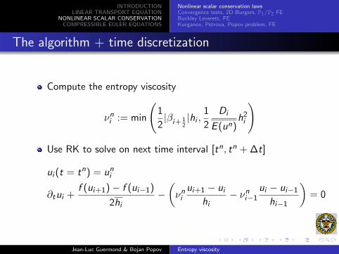
The algorithm + time discretization
Compute the entropy viscosity
νni := min
(1
2|βi+ 1
2|hi ,
1
2
Di
E (un)h2i
)
Use RK to solve on next time interval [tn, tn + ∆t]
ui (t = tn) = uni
∂tui +f (ui+1)− f (ui−1)
2hi
−(νni
ui+1 − ui
hi− νn
i−1
ui − ui−1
hi−1
)= 0
Jean-Luc Guermond & Bojan Popov Entropy viscosity
INTRODUCTIONLINEAR TRANSPORT EQUATION
NONLINEAR SCALAR CONSERVATIONCOMPRESSIBLE EULER EQUATIONS
Nonlinear scalar conservation lawsConvergence tests, 2D Burgers, P1/P2 FEBuckley Leverett, FEKurganov, Petrova, Popov problem, FE
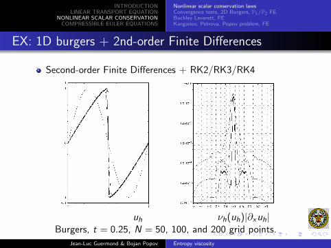
EX: 1D burgers + 2nd-order Finite Differences
Second-order Finite Differences + RK2/RK3/RK4
uh νh(uh)|∂xuh|Burgers, t = 0.25, N = 50, 100, and 200 grid points.
Jean-Luc Guermond & Bojan Popov Entropy viscosity
INTRODUCTIONLINEAR TRANSPORT EQUATION
NONLINEAR SCALAR CONSERVATIONCOMPRESSIBLE EULER EQUATIONS
Nonlinear scalar conservation lawsConvergence tests, 2D Burgers, P1/P2 FEBuckley Leverett, FEKurganov, Petrova, Popov problem, FE
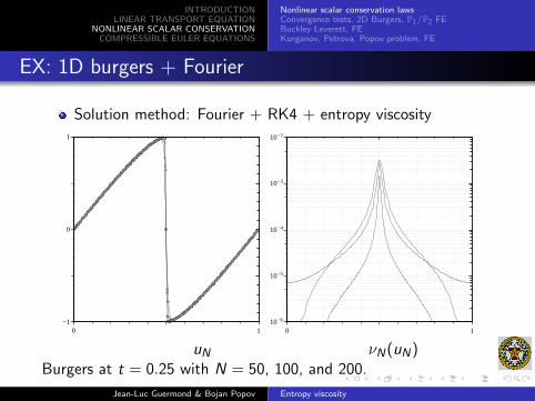
EX: 1D burgers + Fourier
Solution method: Fourier + RK4 + entropy viscosity
Wed Jan 16 09:39:43 2008
0 1−1
0
1
PLOT
X−Axis
Y−
Axi
sWed Jan 16 09:43:35 2008
0 11.0×10⁻⁶
1.0×10⁻⁵
1.0×10⁻⁴
1.0×10⁻³
1.0×10⁻²
PLOT
X−Axis
Y−
Axi
s
uN νN(uN)Burgers at t = 0.25 with N = 50, 100, and 200.
Jean-Luc Guermond & Bojan Popov Entropy viscosity
INTRODUCTIONLINEAR TRANSPORT EQUATION
NONLINEAR SCALAR CONSERVATIONCOMPRESSIBLE EULER EQUATIONS
Nonlinear scalar conservation lawsConvergence tests, 2D Burgers, P1/P2 FEBuckley Leverett, FEKurganov, Petrova, Popov problem, FE
EX: 1D Nonconvex flux + Fourier
Consider ∂t + ∂x f (u) = 0, u(x , 0) = u0(x)
f (u) =
14 u(1− u) if u < 1
2 ,12 u(u − 1) + 3
16 if u ≥ 12 ,
u0(x) =
0, x ∈ (0, 0.25],
1, x ∈ (0.25, 1]
Tue Dec 18 09:45:13 2007
0.3 0.4 0.5 0.6 0.7 0.8 0.9 1−0.1
0
1
1.1
PLOT
X−Axis
Y−
Axi
s
Non-convex flux problemuN at t = 1 with N = 200,400, 800, and 1600.
Jean-Luc Guermond & Bojan Popov Entropy viscosity
INTRODUCTIONLINEAR TRANSPORT EQUATION
NONLINEAR SCALAR CONSERVATIONCOMPRESSIBLE EULER EQUATIONS
Nonlinear scalar conservation lawsConvergence tests, 2D Burgers, P1/P2 FEBuckley Leverett, FEKurganov, Petrova, Popov problem, FE
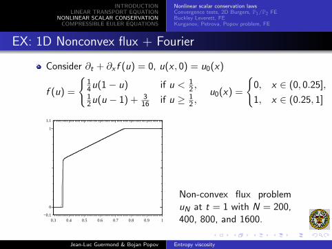
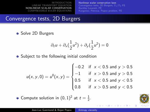
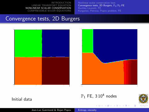
Convergence tests, 2D Burgers
Solve 2D Burgers
∂tu + ∂x(1
2u2) + ∂y (
1
2u2) = 0
Subject to the following initial condition
u(x , y , 0) = u0(x , y) =
−0.2 if x < 0.5 and y > 0.5
−1 if x > 0.5 and y > 0.5
0.5 if x < 0.5 and y < 0.5
0.8 if x > 0.5 and y < 0.5
Compute solution in (0, 1)2 at t = 12 .
Jean-Luc Guermond & Bojan Popov Entropy viscosity
INTRODUCTIONLINEAR TRANSPORT EQUATION
NONLINEAR SCALAR CONSERVATIONCOMPRESSIBLE EULER EQUATIONS
Nonlinear scalar conservation lawsConvergence tests, 2D Burgers, P1/P2 FEBuckley Leverett, FEKurganov, Petrova, Popov problem, FE
Convergence tests, 2D Burgers
Initial dataP1 FE, 3 104 nodes
Jean-Luc Guermond & Bojan Popov Entropy viscosity
INTRODUCTIONLINEAR TRANSPORT EQUATION
NONLINEAR SCALAR CONSERVATIONCOMPRESSIBLE EULER EQUATIONS
Nonlinear scalar conservation lawsConvergence tests, 2D Burgers, P1/P2 FEBuckley Leverett, FEKurganov, Petrova, Popov problem, FE
Convergence tests, 2D Burgers
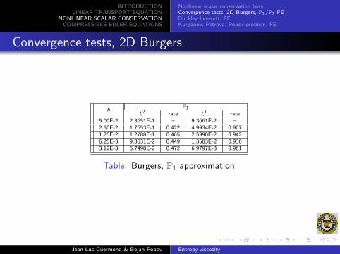
hP1
L2 rate L1 rate5.00E-2 2.3651E-1 – 9.3661E-2 –2.50E-2 1.7653E-1 0.422 4.9934E-2 0.9071.25E-2 1.2788E-1 0.465 2.5990E-2 0.9426.25E-3 9.3631E-2 0.449 1.3583E-2 0.9363.12E-3 6.7498E-2 0.472 6.9797E-3 0.961
Table: Burgers, P1 approximation.
Jean-Luc Guermond & Bojan Popov Entropy viscosity

INTRODUCTIONLINEAR TRANSPORT EQUATION
NONLINEAR SCALAR CONSERVATIONCOMPRESSIBLE EULER EQUATIONS
Nonlinear scalar conservation lawsConvergence tests, 2D Burgers, P1/P2 FEBuckley Leverett, FEKurganov, Petrova, Popov problem, FE
Convergence tests, 2D Burgers
hP2
L2 rate L1 rate5.00E-2 1.8068E-1 – 5.2531E-2 –2.50E-2 1.2956E-1 0.480 2.7212E-2 0.9491.25E-2 9.5508E-2 0.440 1.4588E-2 0.8996.25E-3 6.8806E-2 0.473 7.6435E-3 0.932
Table: Burgers, P2 approximation.
Jean-Luc Guermond & Bojan Popov Entropy viscosity
INTRODUCTIONLINEAR TRANSPORT EQUATION
NONLINEAR SCALAR CONSERVATIONCOMPRESSIBLE EULER EQUATIONS
Nonlinear scalar conservation lawsConvergence tests, 2D Burgers, P1/P2 FEBuckley Leverett, FEKurganov, Petrova, Popov problem, FE
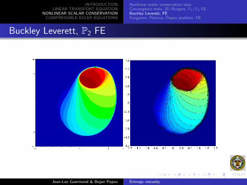
Buckley Leverett, P2 FE
Solve ∂tu + ∂x f (u) + ∂y g(u) = 0.
f (u) = u2
u2+(1−u)2 , g(u) = f (u)(1− 5(1− u)2)
Non-convex fluxes (composite waves)
u(x , y , 0) =
1,
√x2 + y 2 ≤ 0.5
0, else
Jean-Luc Guermond & Bojan Popov Entropy viscosity
INTRODUCTIONLINEAR TRANSPORT EQUATION
NONLINEAR SCALAR CONSERVATIONCOMPRESSIBLE EULER EQUATIONS
Nonlinear scalar conservation lawsConvergence tests, 2D Burgers, P1/P2 FEBuckley Leverett, FEKurganov, Petrova, Popov problem, FE
Buckley Leverett, P2 FE
Jean-Luc Guermond & Bojan Popov Entropy viscosity
INTRODUCTIONLINEAR TRANSPORT EQUATION
NONLINEAR SCALAR CONSERVATIONCOMPRESSIBLE EULER EQUATIONS
Nonlinear scalar conservation lawsConvergence tests, 2D Burgers, P1/P2 FEBuckley Leverett, FEKurganov, Petrova, Popov problem, FE
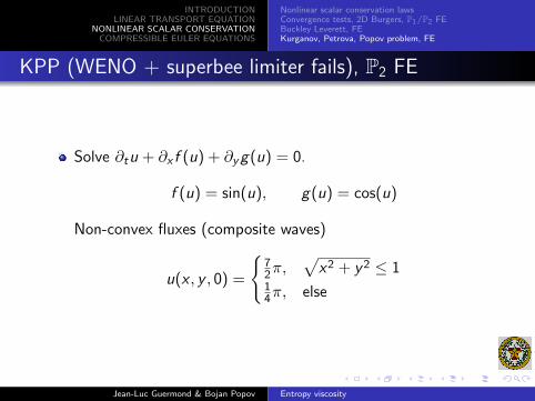
KPP (WENO + superbee limiter fails), P2 FE
Solve ∂tu + ∂x f (u) + ∂y g(u) = 0.
f (u) = sin(u), g(u) = cos(u)
Non-convex fluxes (composite waves)
u(x , y , 0) =
72π,
√x2 + y 2 ≤ 1
14π, else
Jean-Luc Guermond & Bojan Popov Entropy viscosity
INTRODUCTIONLINEAR TRANSPORT EQUATION
NONLINEAR SCALAR CONSERVATIONCOMPRESSIBLE EULER EQUATIONS
Nonlinear scalar conservation lawsConvergence tests, 2D Burgers, P1/P2 FEBuckley Leverett, FEKurganov, Petrova, Popov problem, FE
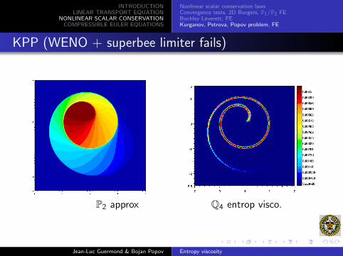
KPP (WENO + superbee limiter fails)
P2 approx Q4 entrop visco.
Jean-Luc Guermond & Bojan Popov Entropy viscosity
INTRODUCTIONLINEAR TRANSPORT EQUATION
NONLINEAR SCALAR CONSERVATIONCOMPRESSIBLE EULER EQUATIONS
Euler equationsThe algorithm1D-2D Tests + Fourier2D tests, P1 finite elements
NONLINEAR SCALAR CONSERVATION EQUATIONS
Leonhard Euler
1 INTRODUCTION2 LINEAR TRANSPORT EQUATION3 NONLINEAR SCALAR CONSERVATION4 COMPRESSIBLE EULER EQUATIONS
Jean-Luc Guermond & Bojan Popov Entropy viscosity
INTRODUCTIONLINEAR TRANSPORT EQUATION
NONLINEAR SCALAR CONSERVATIONCOMPRESSIBLE EULER EQUATIONS
Euler equationsThe algorithm1D-2D Tests + Fourier2D tests, P1 finite elements
Euler flows
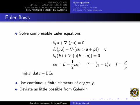
Solve compressible Euler equations
∂tρ+∇·(ρu) = 0
∂t(ρu) +∇·(ρu⊗ u + pI) = 0
∂t(E ) +∇·(u(E + p)) = 0
ρe = E − 1
2ρu2, T = (γ − 1)e T =
p
ρ
Initial data + BCs
Use continuous finite elements of degree p.
Deviate as little possible from Galerkin.
Jean-Luc Guermond & Bojan Popov Entropy viscosity
INTRODUCTIONLINEAR TRANSPORT EQUATION
NONLINEAR SCALAR CONSERVATIONCOMPRESSIBLE EULER EQUATIONS
Euler equationsThe algorithm1D-2D Tests + Fourier2D tests, P1 finite elements
The algorithm
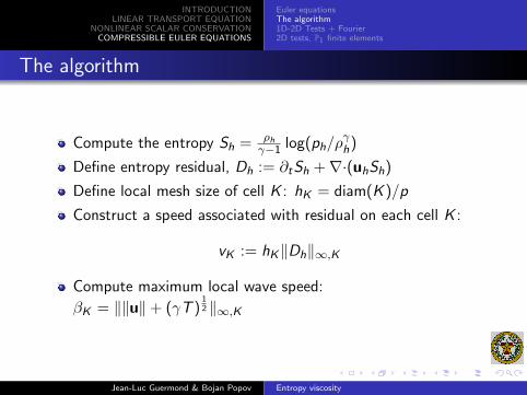
Compute the entropy Sh = ρhγ−1 log(ph/ρ
γh)
Define entropy residual, Dh := ∂tSh +∇·(uhSh)
Define local mesh size of cell K : hK = diam(K )/p
Construct a speed associated with residual on each cell K :
vK := hK‖Dh‖∞,K
Compute maximum local wave speed:
βK = ‖‖u‖+ (γT )12 ‖∞,K
Jean-Luc Guermond & Bojan Popov Entropy viscosity
INTRODUCTIONLINEAR TRANSPORT EQUATION
NONLINEAR SCALAR CONSERVATIONCOMPRESSIBLE EULER EQUATIONS
Euler equationsThe algorithm1D-2D Tests + Fourier2D tests, P1 finite elements
The algorithm
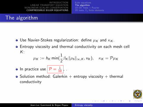
Use Navier-Stokes regularization: define µK and κK .
Entropy viscosity and thermal conductivity on each mesh cellK :
µK := hK min(1
2βK‖ρh‖∞,K , vK ), κK = PµK
In practice use P = 110 , .
Solution method: Galerkin + entropy viscosity + thermalconductivity
Jean-Luc Guermond & Bojan Popov Entropy viscosity
INTRODUCTIONLINEAR TRANSPORT EQUATION
NONLINEAR SCALAR CONSERVATIONCOMPRESSIBLE EULER EQUATIONS
Euler equationsThe algorithm1D-2D Tests + Fourier2D tests, P1 finite elements
1D Euler flows + Fourier
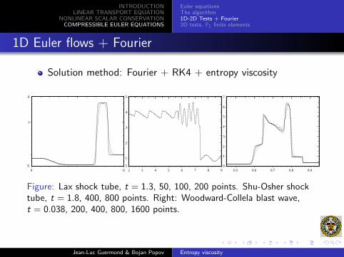
Solution method: Fourier + RK4 + entropy viscosity
Wed Jan 16 11:49:35 2008
0 100.325
1
1.4
PLOT
X−Axis
Y−
Axi
s
Wed Jan 16 15:40:25 2008
2 3 4 5 6 7 8 90.5
1
2
3
4
5
PLOT
X−Axis
Y−
Axi
s
Fri Dec 21 09:24:49 2007
0.5 0.6 0.7 0.8 0.90
1
2
3
4
5
6
7
PLOT
X−Axis
Y−
Axi
s
Figure: Lax shock tube, t = 1.3, 50, 100, 200 points. Shu-Osher shocktube, t = 1.8, 400, 800 points. Right: Woodward-Collela blast wave,t = 0.038, 200, 400, 800, 1600 points.
Jean-Luc Guermond & Bojan Popov Entropy viscosity
INTRODUCTIONLINEAR TRANSPORT EQUATION
NONLINEAR SCALAR CONSERVATIONCOMPRESSIBLE EULER EQUATIONS
Euler equationsThe algorithm1D-2D Tests + Fourier2D tests, P1 finite elements
1D Euler flows + Fourier
Solution method: Fourier + RK4 + entropy viscosity
Wed Jan 16 11:49:35 2008
0 100.325
1
1.4
PLOT
X−Axis
Y−
Axi
s
Wed Jan 16 15:40:25 2008
2 3 4 5 6 7 8 90.5
1
2
3
4
5
PLOT
X−Axis
Y−
Axi
s
Fri Dec 21 09:24:49 2007
0.5 0.6 0.7 0.8 0.90
1
2
3
4
5
6
7
PLOT
X−Axis
Y−
Axi
s
Figure: Lax shock tube, t = 1.3, 50, 100, 200 points. Shu-Osher shocktube, t = 1.8, 400, 800 points. Right: Woodward-Collela blast wave,t = 0.038, 200, 400, 800, 1600 points.
Jean-Luc Guermond & Bojan Popov Entropy viscosity
INTRODUCTIONLINEAR TRANSPORT EQUATION
NONLINEAR SCALAR CONSERVATIONCOMPRESSIBLE EULER EQUATIONS
Euler equationsThe algorithm1D-2D Tests + Fourier2D tests, P1 finite elements
2D Euler flows + Fourier
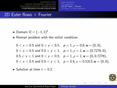
Domain Ω = (−1, 1)2
Rieman problem with the initial condition:
0 < x < 0.5 and 0 < y < 0.5, p = 1, ρ = 0.8,u = (0, 0),
0 < x < 0.5 and 0.5 < y < 1, p = 1, ρ = 1,u = (0.7276, 0),
0.5 < x < 1 and 0 < y < 0.5, p = 1, ρ = 1,u = (0, 0.7276),
0 < x < 0.5 and 0.5 < y < 1, p = 0.4, ρ = 0.5313,u = (0, 0).
Solution at time t = 0.2.
Jean-Luc Guermond & Bojan Popov Entropy viscosity
INTRODUCTIONLINEAR TRANSPORT EQUATION
NONLINEAR SCALAR CONSERVATIONCOMPRESSIBLE EULER EQUATIONS
Euler equationsThe algorithm1D-2D Tests + Fourier2D tests, P1 finite elements
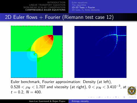
2D Euler flows + Fourier (Riemann test case 12)
Euler benchmark, Fourier approximation: Density (at left),0.528 < ρN < 1.707 and viscosity (at right), 0 < µN < 3.410−3, att = 0.2, N = 400.
Jean-Luc Guermond & Bojan Popov Entropy viscosity
INTRODUCTIONLINEAR TRANSPORT EQUATION
NONLINEAR SCALAR CONSERVATIONCOMPRESSIBLE EULER EQUATIONS
Euler equationsThe algorithm1D-2D Tests + Fourier2D tests, P1 finite elements
Riemann problem test case no 12, P1 FE
movie, Riemann no 12
Jean-Luc Guermond & Bojan Popov Entropy viscosity
INTRODUCTIONLINEAR TRANSPORT EQUATION
NONLINEAR SCALAR CONSERVATIONCOMPRESSIBLE EULER EQUATIONS
Euler equationsThe algorithm1D-2D Tests + Fourier2D tests, P1 finite elements
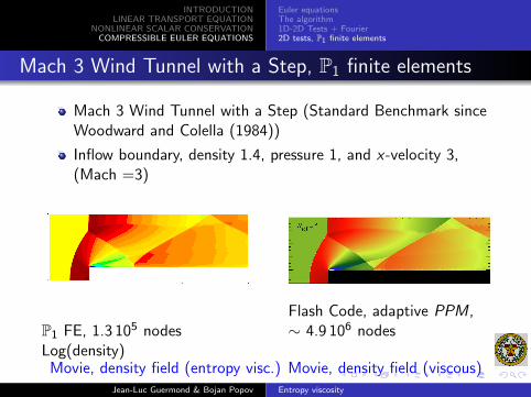
Mach 3 Wind Tunnel with a Step, P1 finite elements
Mach 3 Wind Tunnel with a Step (Standard Benchmark sinceWoodward and Colella (1984))
Inflow boundary, density 1.4, pressure 1, and x-velocity 3,(Mach =3)
P1 FE, 1.3 105 nodesLog(density)
Flash Code, adaptive PPM,∼ 4.9 106 nodes
Movie, density field (entropy visc.) Movie, density field (viscous)
Jean-Luc Guermond & Bojan Popov Entropy viscosity
INTRODUCTIONLINEAR TRANSPORT EQUATION
NONLINEAR SCALAR CONSERVATIONCOMPRESSIBLE EULER EQUATIONS
Euler equationsThe algorithm1D-2D Tests + Fourier2D tests, P1 finite elements
Mach 3 Wind Tunnel with a Step, P1 finite elements
Mach 3 Wind Tunnel with a Step (Standard Benchmark sinceWoodward and Colella (1984))
Inflow boundary, density 1.4, pressure 1, and x-velocity 3,(Mach =3)
P1 FE, 1.3 105 nodesLog(density)
Flash Code, adaptive PPM,∼ 4.9 106 nodes
Movie, density field (entropy visc.) Movie, density field (viscous)Jean-Luc Guermond & Bojan Popov Entropy viscosity
INTRODUCTIONLINEAR TRANSPORT EQUATION
NONLINEAR SCALAR CONSERVATIONCOMPRESSIBLE EULER EQUATIONS
Euler equationsThe algorithm1D-2D Tests + Fourier2D tests, P1 finite elements
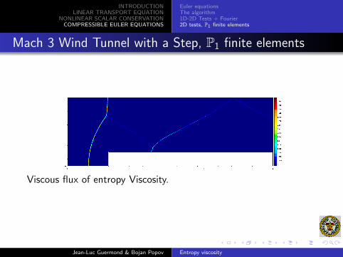
Mach 3 Wind Tunnel with a Step, P1 finite elements
Viscous flux of entropy Viscosity.
Jean-Luc Guermond & Bojan Popov Entropy viscosity
INTRODUCTIONLINEAR TRANSPORT EQUATION
NONLINEAR SCALAR CONSERVATIONCOMPRESSIBLE EULER EQUATIONS
Euler equationsThe algorithm1D-2D Tests + Fourier2D tests, P1 finite elements
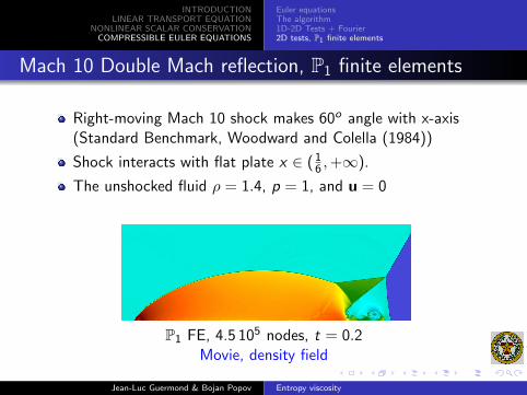
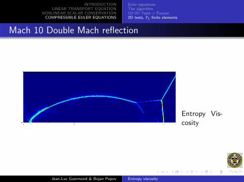
Mach 10 Double Mach reflection, P1 finite elements
Right-moving Mach 10 shock makes 60o angle with x-axis(Standard Benchmark, Woodward and Colella (1984))
Shock interacts with flat plate x ∈ ( 16 ,+∞).
The unshocked fluid ρ = 1.4, p = 1, and u = 0
P1 FE, 4.5 105 nodes, t = 0.2Movie, density field
Jean-Luc Guermond & Bojan Popov Entropy viscosity
INTRODUCTIONLINEAR TRANSPORT EQUATION
NONLINEAR SCALAR CONSERVATIONCOMPRESSIBLE EULER EQUATIONS
Euler equationsThe algorithm1D-2D Tests + Fourier2D tests, P1 finite elements
Mach 10 Double Mach reflection
Entropy Vis-cosity
Jean-Luc Guermond & Bojan Popov Entropy viscosity