J. Fluid Mech. (2014), . 742, doi:10.1017/jfm.2013.641 … · Nychas, Hershey & Brodkey (1973) by visualization showed the occurrence of transverse vortices and suggested that they

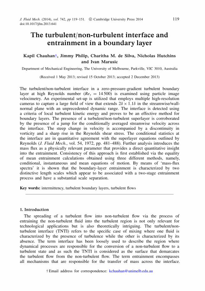
J. Fluid Mech. (2014), vol. 742, pp 119–151. c© Cambridge University Press 2014doi:10.1017/jfm.2013.641

119

The turbulent/non-turbulent interface andentrainment in a boundary layer

Kapil Chauhan†, Jimmy Philip, Charitha M. de Silva, Nicholas Hutchinsand Ivan Marusic

Department of Mechanical Engineering, The University of Melbourne, Parkville, VIC 3010, Australia

(Received 1 May 2013; revised 15 October 2013; accepted 2 December 2013)

The turbulent/non-turbulent interface in a zero-pressure-gradient turbulent boundarylayer at high Reynolds number (Reτ = 14 500) is examined using particle imagevelocimetry. An experimental set-up is utilized that employs multiple high-resolutioncameras to capture a large field of view that extends 2δ× 1.1δ in the streamwise/wall-normal plane with an unprecedented dynamic range. The interface is detected usinga criteria of local turbulent kinetic energy and proves to be an effective method forboundary layers. The presence of a turbulent/non-turbulent superlayer is corroboratedby the presence of a jump for the conditionally averaged streamwise velocity acrossthe interface. The steep change in velocity is accompanied by a discontinuity invorticity and a sharp rise in the Reynolds shear stress. The conditional statistics atthe interface are in quantitative agreement with the superlayer equations outlined byReynolds (J. Fluid Mech., vol. 54, 1972, pp. 481–488). Further analysis introduces themass flux as a physically relevant parameter that provides a direct quantitative insightinto the entrainment. Consistency of this approach is first established via the equalityof mean entrainment calculations obtained using three different methods, namely,conditional, instantaneous and mean equations of motion. By means of ‘mass-fluxspectra’ it is shown that the boundary-layer entrainment is characterized by twodistinctive length scales which appear to be associated with a two-stage entrainmentprocess and have a substantial scale separation.

Key words: intermittency, turbulent boundary layers, turbulent flows

1. Introduction

The spreading of a turbulent flow into non-turbulent flow via the process ofentraining the non-turbulent fluid into the turbulent region is not only relevant fortechnological applications but is also theoretically intriguing. The turbulent/non-turbulent interface (TNTI) refers to the specific case of mixing where one fluid ischaracterized by the presence of turbulence while the other is characterized by itsabsence. The term interface has been loosely used to describe the region wheredynamical processes are responsible for the conversion of a non-turbulent flow to aturbulent state and as such the TNTI is considered as the surface that demarcatesthe turbulent flow from the non-turbulent flow. The term entrainment encompassesall mechanisms that are responsible for the transfer of mass across the interface.

† Email address for correspondence: [email protected]

mailto:[email protected]

120 K. Chauhan, J. Philip, C. M. de Silva, N. Hutchins and I. Marusic

The entrainment mechanisms do not necessarily act at the interface itself and canprecede the interface dynamics; e.g. there exists an induced inflow in the case ofa jet/plume (laminar or turbulent) (e.g. Taylor 1958; Schneider 1981). This inducedvelocity is zero in boundary layers and wakes (Hunt 1994). Following Turner (1986),we consider the mean entrainment velocity as the rate at which external fluid flowsinto the turbulent flow across the mean interface in the laboratory frame of reference.The mean interface velocity is the rate at which the edge of the turbulent flow isspreading out, e.g. the growth in thickness δ or half-height b in boundary layersand jets, respectively. While the mean entrainment dynamics are examined in thefixed laboratory frame of reference, instantaneously the local entrainment velocity isconsidered as the velocity of fluid relative to the transient TNTI (further discussed in§ 7). The entrainment velocity can also be defined based on the flux of concentrationor temperature (Hunt, Rottman & Britter 1984) in flows where the interface ischaracterized by spread of a scalar (e.g. Westerweel et al. 2009). For the case ofentrainment in homogeneous fluids (in contrast to flows with large density differencesor stable stratification, see Turner (1986)) two scenarios emerge: one, where turbulenceis created and the flow has no mean or bulk shear; and two, where the turbulencecan be maintained by a mean shear, such as in jets, wakes and boundary-layerflows. It seems more plausible that the mechanisms involved in the spreading of theturbulent region and entrainment of the non-turbulent fluid into the turbulent coreare different in both cases. In the first case, due to the absence of the mean shearfor the production of turbulence, either the turbulence decays (as in grid-generatedturbulence), or the turbulence has to be continuously maintained by constant agitationat a boundary (such as employing an oscillating grid, see e.g. Holzner et al. (2007)).These are more akin to the turbulent diffusion process (introduced by Taylor 1921). Inthe second case, since the flows have been observed to be dominated by large-scalemotions (such as those observed in jets by Brown & Roshko (1974) and in wakes byCannon, Champagne & Glezer (1993), to name a few), it is not clear how importantthe turbulent diffusion is compared with the role of large-scale motions. This leadsto important questions regarding the roles played by the large-scale, predominantlyinviscid motions and those by the small-scale, diffusive and primarily viscous motions.

In the seminal work of Corrsin & Kistler (1955), two important hypotheses aremade: one, that there is a step change in velocity across the TNTI; and two, thatthe spreading process of the turbulent region in shear flows is similar to turbulentdiffusion (gauged by the observation of wake shadowgraphs, which unfortunately donot show the entrapped non-turbulent fluid inside the turbulent region, as mentionedby Townsend (1976)). After the initial dismay at not finding a velocity jump across theinterface in the 1970s (in boundary-layer flows by Kovasznay, Kibens & Blackwelder1970), more recently it has been observed that, indeed, there does exist a velocityjump at the TNTI of boundary layers (Semin et al. 2011) and in wakes and jets,though over a small but finite region (Bisset, Hunt & Rogers 2002; Westerweelet al. 2005). Regarding the second hypothesis of spreading by turbulent diffusion,it is uncertain whether it is fully correct. If so, it would imply that the large-scalemotions have no role to play in the spreading, which is highly unlikely consideringthat bulk motion is sufficient to determine the spreading and entrainment in shearflows (Townsend 1966). A reconciliation of the large-scale and small-scale points ofview towards entrainment is to some extent provided by Sreenivasan and coworkers(e.g. Sreenivasan, Ramshankar & Meneveau 1989) by showing than an extensivesurface area is created by the large-scale motions such that the total entrainment is

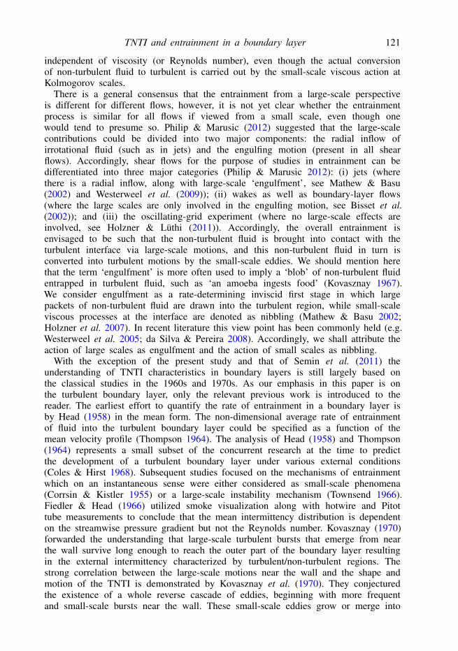
TNTI and entrainment in a boundary layer 121

independent of viscosity (or Reynolds number), even though the actual conversionof non-turbulent fluid to turbulent is carried out by the small-scale viscous action atKolmogorov scales.

There is a general consensus that the entrainment from a large-scale perspectiveis different for different flows, however, it is not yet clear whether the entrainmentprocess is similar for all flows if viewed from a small scale, even though onewould tend to presume so. Philip & Marusic (2012) suggested that the large-scalecontributions could be divided into two major components: the radial inflow ofirrotational fluid (such as in jets) and the engulfing motion (present in all shearflows). Accordingly, shear flows for the purpose of studies in entrainment can bedifferentiated into three major categories (Philip & Marusic 2012): (i) jets (wherethere is a radial inflow, along with large-scale ‘engulfment’, see Mathew & Basu(2002) and Westerweel et al. (2009)); (ii) wakes as well as boundary-layer flows(where the large scales are only involved in the engulfing motion, see Bisset et al.(2002)); and (iii) the oscillating-grid experiment (where no large-scale effects areinvolved, see Holzner & Lüthi (2011)). Accordingly, the overall entrainment isenvisaged to be such that the non-turbulent fluid is brought into contact with theturbulent interface via large-scale motions, and this non-turbulent fluid in turn isconverted into turbulent motions by the small-scale eddies. We should mention herethat the term ‘engulfment’ is more often used to imply a ‘blob’ of non-turbulent fluidentrapped in turbulent fluid, such as ‘an amoeba ingests food’ (Kovasznay 1967).We consider engulfment as a rate-determining inviscid first stage in which largepackets of non-turbulent fluid are drawn into the turbulent region, while small-scaleviscous processes at the interface are denoted as nibbling (Mathew & Basu 2002;Holzner et al. 2007). In recent literature this view point has been commonly held (e.g.Westerweel et al. 2005; da Silva & Pereira 2008). Accordingly, we shall attribute theaction of large scales as engulfment and the action of small scales as nibbling.

With the exception of the present study and that of Semin et al. (2011) theunderstanding of TNTI characteristics in boundary layers is still largely based onthe classical studies in the 1960s and 1970s. As our emphasis in this paper is onthe turbulent boundary layer, only the relevant previous work is introduced to thereader. The earliest effort to quantify the rate of entrainment in a boundary layer isby Head (1958) in the mean form. The non-dimensional average rate of entrainmentof fluid into the turbulent boundary layer could be specified as a function of themean velocity profile (Thompson 1964). The analysis of Head (1958) and Thompson(1964) represents a small subset of the concurrent research at the time to predictthe development of a turbulent boundary layer under various external conditions(Coles & Hirst 1968). Subsequent studies focused on the mechanisms of entrainmentwhich on an instantaneous sense were either considered as small-scale phenomena(Corrsin & Kistler 1955) or a large-scale instability mechanism (Townsend 1966).Fiedler & Head (1966) utilized smoke visualization along with hotwire and Pitottube measurements to conclude that the mean intermittency distribution is dependenton the streamwise pressure gradient but not the Reynolds number. Kovasznay (1970)forwarded the understanding that large-scale turbulent bursts that emerge from nearthe wall survive long enough to reach the outer part of the boundary layer resultingin the external intermittency characterized by turbulent/non-turbulent regions. Thestrong correlation between the large-scale motions near the wall and the shape andmotion of the TNTI is demonstrated by Kovasznay et al. (1970). They conjecturedthe existence of a whole reverse cascade of eddies, beginning with more frequentand small-scale bursts near the wall. These small-scale eddies grow or merge into


larger scales and eventually reach the non-turbulent flow at a lesser frequency thantheir origin. These views are consistent with the views of Adrian (2007) where thebulges/valleys in the outer region are interpreted as large-scale motions in the formof packets of attached eddies that extend to the edge of the boundary layer. However,it is noted that the large-scale bulges in outer region could also be a consequence ofan instability mechanism (Townsend 1966).

Nychas, Hershey & Brodkey (1973) by visualization showed the occurrence oftransverse vortices and suggested that they are one of the mechanisms that inducehigher-speed fluid towards the inner zones. The characteristics of the leading andtrailing edges of the turbulent bulges in the outer part of the boundary layer areexamined by Hedley & Keffer (1974a). They found that sharp changes occurthrough the ‘backs’, i.e. the TNTI when one moves from the turbulent zone tothe non-turbulent zone in the direction opposite to the flow. On the other hand the‘fronts’ exhibit a more diffusive behaviour in their analysis. Chen & Blackwelder(1978) used temperature as a passive contaminant in order to study the large-scalestructure in the outer part. They confirmed the presence of a sharp interface byconditional averages of temperature profiles. Mean intermittency measurements usingconcentration sources from two different elevations in the boundary layer wereperformed by Fackrell & Robins (1982) while intermittency characteristics underdifferent free-stream turbulence levels are documented by Hancock & Bradshaw(1989). Most of these studies are at relatively low Reynolds numbers and lackedcomprehensive measurement apparatus to track the instantaneous TNTI in twodimensions.

Accordingly, there are two main objectives of the present work. First, to quantify theinterface properties (particularly the velocity jump across it) in the turbulent boundarylayer at a relatively high Reynolds number and discuss its implications. Since similarstudies do exist for wakes and jet, the present study will provide insight for theboundary-layer flow and complete the list by including the wall-shear flow. Second,to understand the entrainment of the fluid across the interface from the large-scaleand small-scale points of view. To this end, we shall calculate mass entrainment usingthree methods and also introduce the ‘mass-flux spectra’ to differentiate the lengthscales involved in the entrainment.

The outline of the paper is as follows: § 2 describes the experimental setup andthe particle image velocimetry (PIV) measurements at high Reynolds number; § 3describes the procedure to determine the interface using velocity data from PIV ina turbulent boundary layer; § 4 provides the spatial statistics of the interface; theconditionally averaged statistics relative to the interface location are presented in § 5;the instantaneous and mean mass flux across the interface and its relevant lengthscales are examined in § 7; a summary and conclusions are included in § 8. Thenotation adopted is as follows. The streamwise and wall-normal axes are representedby x and z, respectively, in the Cartesian system. The distance along the interfaceis s (see figure 1a). The instantaneous streamwise velocity, wall-normal velocity andspanwise vorticity are represented by U, W and Ωy, respectively. The correspondingmean components are denoted as U, W and Ωy and lowercase symbols are usedfor fluctuating components (u, w and ωy). The superscript ‘+’ indicates the scalingby inner length (ν/uτ ) and velocity (uτ ) scales, where ν and uτ are the kinematicviscosity and friction velocity, respectively. The subscript ‘i’ denotes quantities atthe interface. Further notation for the conditional averages and mass flux will beintroduced in the relevant sections.


x

z

s

21 m from the trip

Non-turbulent

Turbulent

Inte

rfac

e,

2

4

6

102 103 1040

8(a () b)

10

15

20

25

30

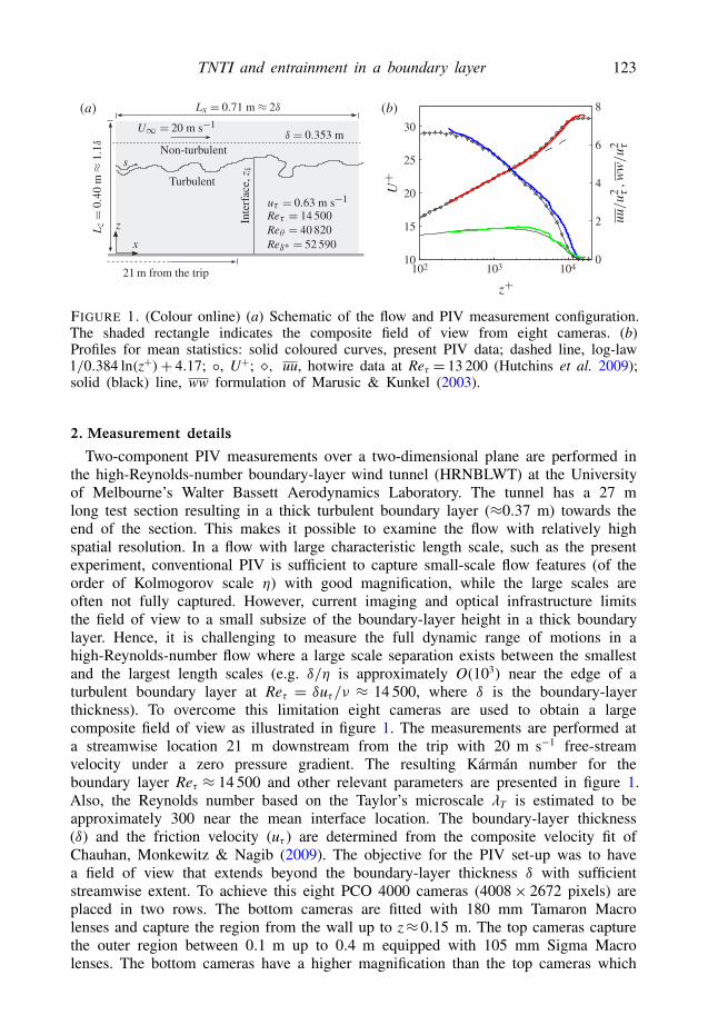
FIGURE 1. (Colour online) (a) Schematic of the flow and PIV measurement configuration.The shaded rectangle indicates the composite field of view from eight cameras. (b)Profiles for mean statistics: solid coloured curves, present PIV data; dashed line, log-law1/0.384 ln(z+)+ 4.17; , U+; , uu, hotwire data at Reτ = 13 200 (Hutchins et al. 2009);solid (black) line, ww formulation of Marusic & Kunkel (2003).

2. Measurement details

Two-component PIV measurements over a two-dimensional plane are performed inthe high-Reynolds-number boundary-layer wind tunnel (HRNBLWT) at the Universityof Melbourne’s Walter Bassett Aerodynamics Laboratory. The tunnel has a 27 mlong test section resulting in a thick turbulent boundary layer (≈0.37 m) towards theend of the section. This makes it possible to examine the flow with relatively highspatial resolution. In a flow with large characteristic length scale, such as the presentexperiment, conventional PIV is sufficient to capture small-scale flow features (of theorder of Kolmogorov scale η) with good magnification, while the large scales areoften not fully captured. However, current imaging and optical infrastructure limitsthe field of view to a small subsize of the boundary-layer height in a thick boundarylayer. Hence, it is challenging to measure the full dynamic range of motions in ahigh-Reynolds-number flow where a large scale separation exists between the smallestand the largest length scales (e.g. δ/η is approximately O(103) near the edge of aturbulent boundary layer at Reτ = δuτ/ν ≈ 14 500, where δ is the boundary-layerthickness). To overcome this limitation eight cameras are used to obtain a largecomposite field of view as illustrated in figure 1. The measurements are performed ata streamwise location 21 m downstream from the trip with 20 m s−1 free-streamvelocity under a zero pressure gradient. The resulting Kármán number for theboundary layer Reτ ≈ 14 500 and other relevant parameters are presented in figure 1.Also, the Reynolds number based on the Taylor’s microscale λT is estimated to beapproximately 300 near the mean interface location. The boundary-layer thickness(δ) and the friction velocity (uτ ) are determined from the composite velocity fit ofChauhan, Monkewitz & Nagib (2009). The objective for the PIV set-up was to havea field of view that extends beyond the boundary-layer thickness δ with sufficientstreamwise extent. To achieve this eight PCO 4000 cameras (4008× 2672 pixels) areplaced in two rows. The bottom cameras are fitted with 180 mm Tamaron Macrolenses and capture the region from the wall up to z≈0.15 m. The top cameras capturethe outer region between 0.1 m up to 0.4 m equipped with 105 mm Sigma Macrolenses. The bottom cameras have a higher magnification than the top cameras which


is suitable for wall-bounded shear flows where small-scale motions are prominentin the near-wall region. The resulting magnification for the top and bottom camerasare 100 and 60 µm per pixel, respectively. An interrogation window of 24 × 24pixels is used for the top cameras with 50 % overlap, while the bottom cameraused an interrogation window of 16 × 16 pixels. In our measurements the ratio ofTaylor microscale (λT) to the interrogation window size (∆i) is approximately three(λT/∆i ≈ 3), while the ratio of interrogation window size to the Kolmogorov scale isapproximately six (∆i/η ≈ 6, η ≈ 16ν/uτ in the outer region). The bottom camerashave the same spacing between vectors as that of the top camera. An overlap ofat least 2 cm between cameras in real space ensured that the vector field fromeach camera is suitably merged. Illumination is achieved by a laser sheet beamedfrom underneath the glass floor, close to the spanwise centre of the tunnel, using aSpectra Physics ‘QuantaRay’ Nd:YAG laser rated 400 mJ at 532 nm. A total of 1440synchronous images are acquired by all eight cameras at 2 Hz. The double-frameimages are interrogated using fast Fourier transform (FFT)-based cross-correlationwith standard algorithms such as multipass, multigrid and second-order correlation forspurious correction (Hart 2000). After discarding images with poor seeding densityand spurious vectors a total of 1250 images are used for the present analysis with590× 328 vectors over a streamwise/wall-normal region of 2δ × 1.1δ. Further detailsof the experiments can be found in de Silva et al. (2012).

The results for the mean statistics are shown in figure 1(b) as solid lines for thepresent study. The mean streamwise velocity U and its variance uu are comparedwith hotwire measurement in the same facility at the nearest Reynolds number.Measurements from PIV are in good agreement with the hotwire for the mean flow.The full logarithmic overlap region is measured. The region below z+= 200 could notbe measured by PIV as meaningful and consistent correlation could not be obtainedin this region due to reflection of the laser sheet on the glass wall. The varianceof the wall-normal fluctuations ww is compared with the similarity formulation ofMarusic & Kunkel (2003) at an equivalent Reynolds number and is found to be ingood agreement with their formulation. One can also notice a slight discontinuitynear z+ = 6000 in the profiles for the variance which is due to marginally differentspatial resolution of the top and bottom cameras. Overall we find that the present setof PIV measurements agree well with the previous data and provides converged firstand second-order statistics.

3. Interface detection

The approach to detect the TNTI in a flow depends on the technique employed formeasuring or observing the flow. In the intermittent region single-point techniquessuch as hotwire anemometry would measure a velocity time series that is turbulent incertain segments and non-turbulent in the rest. In the turbulent zones the localfluctuations are random and with amplitude much larger than the free-streamturbulence intensity, while in the non-turbulent zone the signal is essentially thefree stream. For a velocity signal the turbulent/non-turbulent zones could be identifiedby adopting a threshold technique, where a detector function is calculated fromthe magnitude or time/space derivative of the velocity. Hedley & Keffer (1974b)has listed various turbulence detector functions for time-series measurements. Inspatial techniques such as PIV or planar visualization one obtains information overa two-dimensional plane and the temporal resolution of velocity measurement istypically not sufficient for turbulent flows at high Reynolds numbers. For such


experiments, conventionally the TNTI is determined either by detecting the scalarconcentration in a flow or isolating the rotational flow from the irrotational flow (e.g.Sandham et al. 1988; Prasad & Sreenivasan 1989; Bisset et al. 2002; Westerweelet al. 2009). In the present experiments PIV only provides the velocity informationthroughout the field of view. The seeding particles are present throughout theregion of interest and therefore one cannot detect the instantaneous interface ofthe flow using particle density (or pixel intensity) as a criteria. Consequently wedetermine the interface from the velocity information. Typically a threshold onthe vorticity magnitude has been utilized to distinguish the irrotational flow fromthe turbulent regions in jets (Westerweel et al. 2005; Khashehchi et al. 2013) andwakes (Bisset et al. 2002). However, in an experimental turbulent boundary layer thefree-stream turbulence intensity is not precisely zero (unlike jets) and hence fixing athreshold vorticity magnitude can be challenging even if there is a slight noise in thevelocity measurements. Anand, Boersma & Agrawal (2009) compared four differentapproaches including a vorticity and a velocity criteria to identify the TNTI (althoughthe velocity criteria they used is different to the present approach). In their study theyfound that although instantaneously the detected interface differs for different criteria,the conditionally averaged statistics are in acceptable agreement with each other. Inthe current study the local variance of velocity fluctuations is used to distinguish theturbulent from non-turbulent regions. It will be shown in the forthcoming discussionthat for turbulent boundary layers the approach adopted here to find an interface froma two-dimensional vector field is sufficiently effective.

At the interface and over a small region above the interface the streamwiseconvection velocity can be considered to be approximately U∞ (e.g. Corrsin &Kistler 1955; Fiedler & Head 1966; Kovasznay et al. 1970; Jiménez et al. 2010).A local turbulent kinetic energy in the frame of reference moving with U∞, over a3× 3 grid is then defined as

k= 100× 19 U2∞

1∑m,n=−1

[(Um,n −U∞)2 + (Wm,n)2]. (3.1)

In the region above the interface, k should be nearly the same as the free-streamturbulence intensity (uu/U2

∞) of the tunnel, while below the interface k would increasevery rapidly as one approaches the wall. This metric provides a direct physical basisto distinguish between the turbulent regions where the kinetic energy of fluctuations ishigh from the non-turbulent regions where the kinetic energy of fluctuations is nearlyzero. Figure 2(a) shows contours of ln k using (3.1). The kinetic energy k is shown ona logarithmic scale for clarity as it varies from nearly zero in the potential region to100 at the wall. In the free stream k≈ 0 and hence the contours of ln k uniformly takea large negative value in this region. A rapid rise in k is seen as one approaches thewall. The flow can be then characterized as turbulent beyond a certain threshold fork. The kinetic energy also appears to be space filling in the turbulent regions wherethe contours have a darker shade. In contrast, for a high-Reynolds-number flow, theinstantaneous vorticity appears in concentrated volume fractions of the total volume(e.g. see figure 3a of Jiménez et al. 2010). Furthermore, the instantaneous vorticityis not identically zero in the potential region because of finite free-stream turbulenceintensity in experiments and measurement noise. These characteristics favour using thekinetic energy criteria to determine the interface in our study. The implementation ofsuch a criteria is described below.


5000

10 000

10

12

14

16

18

20

–1.0

–0.5

0

0.5

1.0

1.5

2.0

0

0.2

0.4

0.6

0.8

1.0

0

5000

10 000

15 000

0

15 000

(a)

(b)

0

0.2

0.4

0.6

0.8

1.0

0 5000 10 000 15 000 20 000 25 000

0.2 0.4 0.6 0.8 1.0 1.2 1.4 1.6 1.8 2.0

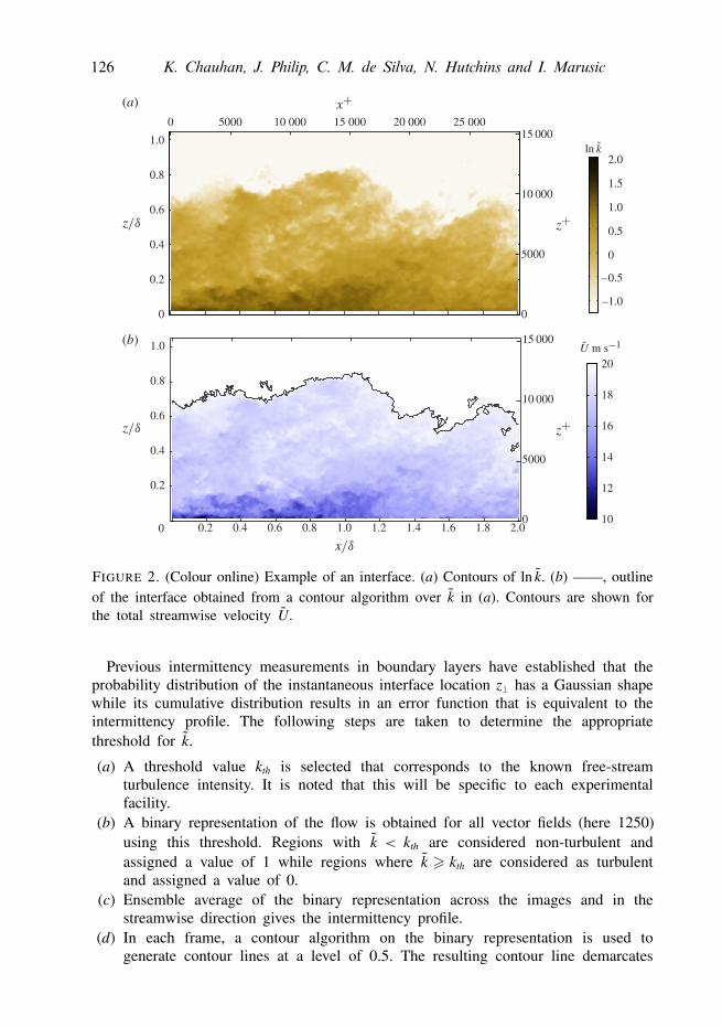
FIGURE 2. (Colour online) Example of an interface. (a) Contours of ln k. (b) ——, outlineof the interface obtained from a contour algorithm over k in (a). Contours are shown forthe total streamwise velocity U.

Previous intermittency measurements in boundary layers have established that theprobability distribution of the instantaneous interface location zi has a Gaussian shapewhile its cumulative distribution results in an error function that is equivalent to theintermittency profile. The following steps are taken to determine the appropriatethreshold for k.

(a) A threshold value kth is selected that corresponds to the known free-streamturbulence intensity. It is noted that this will be specific to each experimentalfacility.

(b) A binary representation of the flow is obtained for all vector fields (here 1250)using this threshold. Regions with k < kth are considered non-turbulent andassigned a value of 1 while regions where k > kth are considered as turbulentand assigned a value of 0.

(c) Ensemble average of the binary representation across the images and in thestreamwise direction gives the intermittency profile.

(d) In each frame, a contour algorithm on the binary representation is used togenerate contour lines at a level of 0.5. The resulting contour line demarcates


the turbulent and non-turbulent regions. The coordinate set I = [xi, zi] of thecontour line is the interface.

(e) The local interface positions from all vector fields are determined and employedto obtain its mean (Zi) and standard deviation (σi).

(f ) Various values of the kinetic energy thresholds are checked in increments of 0.01such that the following two conditions are satisfied: (i) the resulting intermittencyprofile from step (c) agrees with an error function; and (ii) the mean and standarddeviation of zi from step (e) are such that Zi + 3σi ≈ δ. This ensures that theintermittency beyond z= δ is essentially zero and consistent with the definitionof the boundary-layer thickness.

From the above procedure a threshold of kth = 0.12 is determined for the presentdata. It is re-emphasized that the chosen threshold value depends on the free-streamturbulence intensity of the wind tunnel as well as any noise in the PIV measurements.The present threshold of 0.12 is found to produce a good agreement between theintermittency profile from the PIV data and those from hotwire data (see § 4). Theresults pertaining to the small- and large-scale characteristics of entrainment in § 7are qualitatively robust to this threshold value. An example of an interface determinedby this approach is plotted in figure 2(b) over contours of instantaneous streamwisevelocity field.

The instantaneous interface is clearly not smooth. The actual boundary-layerinterface is a two-dimensional surface, however with planar PIV we can onlycapture a two-dimensional vector field and thereby the interface here is a line inthe streamwise/wall-normal plane. We shall often refer to this as the interface outline.In the example shown, the interface outline resides well below the boundary-layerthickness δ, and this is the typical case as δ is the limit beyond which turbulentfluctuations cease to exist. It is seen that instantaneously the interface locationrelative to the wall varies significantly over the streamwise distance of 2δ. Large-scaleindentations are present in the outline giving rise to the appearance of bulges andvalleys. The interface location is also not monotonic in x, i.e. the interface foldsback onto itself and hence at a particular streamwise location multiple TNTIs couldbe present. Large-scale indentations are present along with smaller pockets andfurther detailed examination shows that the outline is seemingly ‘wrinkled’ at evensmaller scales. In many vector fields, ‘pockets’ of non-turbulent fluid are identifiedbelow the interface, surrounded completely by turbulent fluid. Similar pockets ofturbulent fluid are also seen in the potential flow region. These pockets are probablythree-dimensional fluid zones that are engulfed and in the process of becoming partof the turbulent flow due to the presence of vorticity at its boundary. In this paperwe will solely focus on the entrainment that occurs on the interface that extends fromthe left edge to the right edge of the vector field.

4. Geometrical properties of the interfaceIn this section we examine the characteristics of the interface primarily for its

geometrical aspects. The probability density function (p.d.f.) for the instantaneousinterface height zi is plotted in figure 3(a). The p.d.f. of zi is obtained aftercombining the coordinate set I = [xi, zi] from all vector fields. The p.d.f. exhibits anormal distribution with a mean interface location Zi = 0.67δ and standard deviationσi = 0.11δ. The mean interface location and its width agrees well the previousexperiments listed in table 1. (Note that earlier studies adopted δ99 or δ99.5 as thedefinition of the boundary-layer thickness which are smaller than δ used in this paper


Z

0

0.2

0.5

0.8

1.0

0

1

2

3

4

5

6

Nimages

(a () b)

(c () d )

0.2

0.4

0.6

0.8

0

0.99

0.4 0.67 0.9 1.00.20 0.4 0.67 0.9 1.00.20

102104

105

103 104 1 250 500 750 1000 1250

FIGURE 3. (Colour online) Properties of the interface. (a) —— (shown in red online),p.d.f. P of zi; − − − (shown in blue online), normal distribution with mean equalto 0.67 and standard deviation as 0.11; —— (shown in black), U/U∞. (b) Intermittencyγ : symbols, γ from hotwire data of Kulandaivelu (2012); —— (shown in red online),cumulative distribution C of zi; − − − (shown in blue online), γ from streamwiseaveraging of turbulent/non-turbulent regions of PIV data. (c) , number of boxes versusbox size in inner units; —— (shown in red online), least-squares fit to ln b+Nb versusln b+. (d) Gray •, length of the interface outline over a unit streamwise length; ——(shown in red online), cumulative average of `s/Lx→ 3 for 1250 vector fields.

for a particular Reynolds number.) A normal distribution fitted to the data provides avery good model for the p.d.f. of zi except for deviation near the tail on either sideof the mean (which is evident on a logarithmic vertical axis). It is noted that theinterface resides mostly below z = δ (as seen in figure 2). This is obvious from thefact that the boundary-layer thickness δ is the outermost boundary of the turbulentregion beyond which fully non-turbulent flow exists. If the instantaneous interfacereaches above δ it would imply that the turbulent region has extended beyond δ andsuch a scenario is inconsistent with a proper definition of δ. The interface identifiedin the current study using criteria of (3.1) rarely reaches beyond z = δ which is


Reτ = δuτ/ν Zi/δ σi/δ σi/Zi

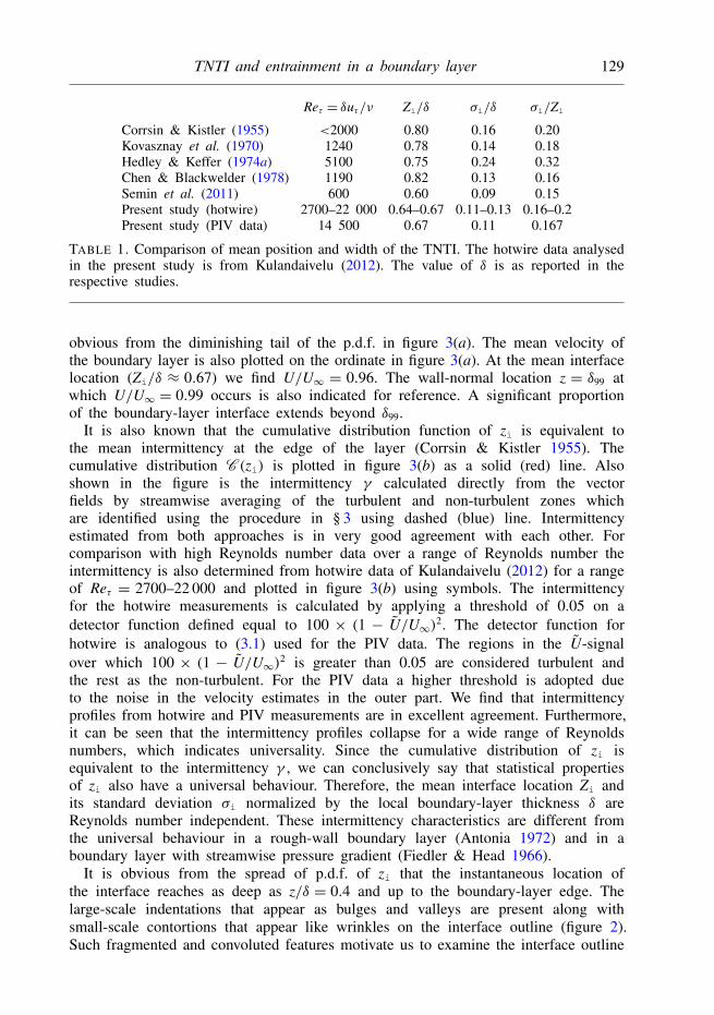
Corrsin & Kistler (1955) <2000 0.80 0.16 0.20Kovasznay et al. (1970) 1240 0.78 0.14 0.18Hedley & Keffer (1974a) 5100 0.75 0.24 0.32Chen & Blackwelder (1978) 1190 0.82 0.13 0.16Semin et al. (2011) 600 0.60 0.09 0.15Present study (hotwire) 2700–22 000 0.64–0.67 0.11–0.13 0.16–0.2Present study (PIV data) 14 500 0.67 0.11 0.167

TABLE 1. Comparison of mean position and width of the TNTI. The hotwire data analysedin the present study is from Kulandaivelu (2012). The value of δ is as reported in therespective studies.

obvious from the diminishing tail of the p.d.f. in figure 3(a). The mean velocity ofthe boundary layer is also plotted on the ordinate in figure 3(a). At the mean interfacelocation (Zi/δ ≈ 0.67) we find U/U∞ = 0.96. The wall-normal location z = δ99 atwhich U/U∞ = 0.99 occurs is also indicated for reference. A significant proportionof the boundary-layer interface extends beyond δ99.

It is also known that the cumulative distribution function of zi is equivalent tothe mean intermittency at the edge of the layer (Corrsin & Kistler 1955). Thecumulative distribution C (zi) is plotted in figure 3(b) as a solid (red) line. Alsoshown in the figure is the intermittency γ calculated directly from the vectorfields by streamwise averaging of the turbulent and non-turbulent zones whichare identified using the procedure in § 3 using dashed (blue) line. Intermittencyestimated from both approaches is in very good agreement with each other. Forcomparison with high Reynolds number data over a range of Reynolds number theintermittency is also determined from hotwire data of Kulandaivelu (2012) for a rangeof Reτ = 2700–22 000 and plotted in figure 3(b) using symbols. The intermittencyfor the hotwire measurements is calculated by applying a threshold of 0.05 on adetector function defined equal to 100 × (1 − U/U∞)2. The detector function forhotwire is analogous to (3.1) used for the PIV data. The regions in the U-signalover which 100 × (1 − U/U∞)2 is greater than 0.05 are considered turbulent andthe rest as the non-turbulent. For the PIV data a higher threshold is adopted dueto the noise in the velocity estimates in the outer part. We find that intermittencyprofiles from hotwire and PIV measurements are in excellent agreement. Furthermore,it can be seen that the intermittency profiles collapse for a wide range of Reynoldsnumbers, which indicates universality. Since the cumulative distribution of zi isequivalent to the intermittency γ , we can conclusively say that statistical propertiesof zi also have a universal behaviour. Therefore, the mean interface location Zi andits standard deviation σi normalized by the local boundary-layer thickness δ areReynolds number independent. These intermittency characteristics are different fromthe universal behaviour in a rough-wall boundary layer (Antonia 1972) and in aboundary layer with streamwise pressure gradient (Fiedler & Head 1966).

It is obvious from the spread of p.d.f. of zi that the instantaneous location ofthe interface reaches as deep as z/δ = 0.4 and up to the boundary-layer edge. Thelarge-scale indentations that appear as bulges and valleys are present along withsmall-scale contortions that appear like wrinkles on the interface outline (figure 2).Such fragmented and convoluted features motivate us to examine the interface outline


for fractal characteristics. The notion that the TNTI adheres to fractal geometry wasfirst demonstrated experimentally by Sreenivasan & Meneveau (1986). Recently deSilva et al. (2013) demonstrated that the fractal dimension of the TNTI in a turbulentboundary layer at high Reynolds numbers is between 2.3 and 2.4. They utilized thekinetic energy criteria to determine the TNTI for two different Reynolds numbersand found that the fractal characteristics are robust to the chosen kinetic energythreshold. Here we briefly discuss the fractal nature of the TNTI to motivate theexposition of multiscale entrainment phenomena that is discussed in § 7. The fractaldimension of the interface is calculated using the box-counting method describedby Prasad & Sreenivasan (1989) and is only briefly discussed here. The field ofview is divided into square boxes of a certain size (box size, b+) and we count thenumber of boxes (Nb) within which the interface is present. Each box size can beconsidered as a measuring unit. The procedure is repeated for different box sizesover the 1250 interface outlines considered in our analysis. The resulting averagevariation of Nb versus b+ appears linear on a log–log plot. However, deviations fromthe linear slope are hard to observe in the log–log plot of Nb versus b+. Therefore,we multiply Nb with b+ to plot b+Nb versus b+ in figure 3(c). It is intuitive that asthe size of box decreases the number of boxes required to measure the interface ofa particular length increases. The linear trend of ln(b+Nb) versus ln b+ implies thatNb∝ (b+)−Df+1. The slope is determined by fitting within the bounds λ+T < b+< 0.2δ+.The slope of the linear trend in figure 3(c) is approximately −0.3 which results in thefractal dimension being Df ≈ 2.3. This value of the fractal dimension of the interface,within experimental error, is in good agreement with the values obtained in previousstudies where the interface was identified using different approaches (Sreenivasanet al. 1989; Meneveau & Sreenivasan 1990). In figure 3(c) we have also shown twovertical lines at λ+T ≈ 300 and 0.85δ+. These represent the small- and large-scaleestimates of entraining motions derived in § 7 and will be discussed therein. It isnoted in figure 3(c) that approximately below the Taylor microscale the scales of theinterface deviate from the fractal characteristic. On the other hand, at the outer limitof figure 3(c) the data fails to show a clear fractal behaviour. This is a limitationsuffered in obtaining converged statistics corresponding to large scales. The largestbox size used in calculating Nb corresponds to 400 vectors and is equivalent to 1.36δ.For a box size in this range the box count is saturated at two as only two boxeswould be required to occupy the interface over a domain of 2δ × 1.1δ. One wouldneed an even larger field of view than the current experiment to obtain the convergedfractal behaviour at box size of O(δ).

In the present experimental set-up we have a field of view that is 2δ long in thestreamwise direction. It is obvious from figure 2 and the fractal characteristic of theinterface that the length of the interface measured along on the path I=[xi, zi] will begreater than the streamwise distance Lx (=2δ). The length of interface `s is calculatedin all PIV vector fields and normalized by the streamwise distance Lx and are shownin figure 3(d). The interface length is at least twice the streamwise distance and isoften as high as 5Lx. This figure quantifies the contorted feature of the interfaceoutline. Both large-scale bulges/valleys and small-scale wrinkles contribute to theincreased length. The moving average of interface length per unit streamwise distancefrom all 1250 vector fields quickly converges to 3.0, indicated by the solid (shown inred online) line in figure 3(d). In theory, if we had access to similar measurementsin the spanwise/wall-normal plane and the interface outline was determined on thisplane, then the fractal dimension of the interface would also equal 2.3 (see § 2.2 in


0

0.2

0.4

0.6

0.8

1.0

0.41.0 –0.02 0 0.02 0.040.90.80.70.6 0.60.81.00

0.2

0.4

0.6

0.8

1.0

(a () b () c)

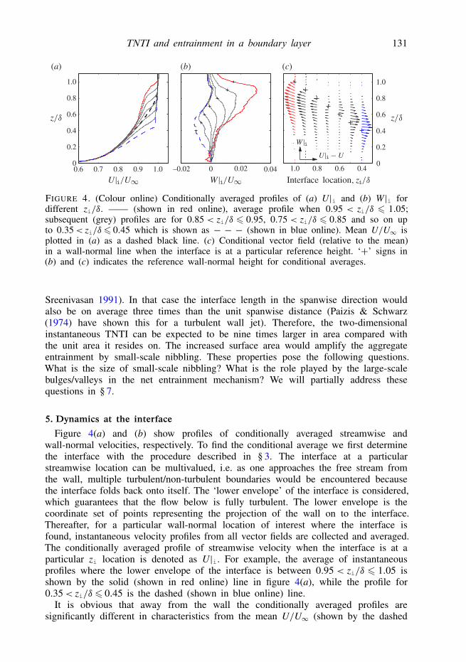
FIGURE 4. (Colour online) Conditionally averaged profiles of (a) U|i and (b) W|i fordifferent zi/δ. —— (shown in red online), average profile when 0.95 < zi/δ 6 1.05;subsequent (grey) profiles are for 0.85 < zi/δ 6 0.95, 0.75 < zi/δ 6 0.85 and so on upto 0.35< zi/δ6 0.45 which is shown as − − − (shown in blue online). Mean U/U∞ isplotted in (a) as a dashed black line. (c) Conditional vector field (relative to the mean)in a wall-normal line when the interface is at a particular reference height. ‘+’ signs in(b) and (c) indicates the reference wall-normal height for conditional averages.

Sreenivasan 1991). In that case the interface length in the spanwise direction wouldalso be on average three times than the unit spanwise distance (Paizis & Schwarz(1974) have shown this for a turbulent wall jet). Therefore, the two-dimensionalinstantaneous TNTI can be expected to be nine times larger in area compared withthe unit area it resides on. The increased surface area would amplify the aggregateentrainment by small-scale nibbling. These properties pose the following questions.What is the size of small-scale nibbling? What is the role played by the large-scalebulges/valleys in the net entrainment mechanism? We will partially address thesequestions in § 7.

5. Dynamics at the interface

Figure 4(a) and (b) show profiles of conditionally averaged streamwise andwall-normal velocities, respectively. To find the conditional average we first determinethe interface with the procedure described in § 3. The interface at a particularstreamwise location can be multivalued, i.e. as one approaches the free stream fromthe wall, multiple turbulent/non-turbulent boundaries would be encountered becausethe interface folds back onto itself. The ‘lower envelope’ of the interface is considered,which guarantees that the flow below is fully turbulent. The lower envelope is thecoordinate set of points representing the projection of the wall on to the interface.Thereafter, for a particular wall-normal location of interest where the interface isfound, instantaneous velocity profiles from all vector fields are collected and averaged.The conditionally averaged profile of streamwise velocity when the interface is at aparticular zi location is denoted as U|i. For example, the average of instantaneousprofiles where the lower envelope of the interface is between 0.95 < zi/δ 6 1.05 isshown by the solid (shown in red online) line in figure 4(a), while the profile for0.35< zi/δ 6 0.45 is the dashed (shown in blue online) line.

It is obvious that away from the wall the conditionally averaged profiles aresignificantly different in characteristics from the mean U/U∞ (shown by the dashed


black line). For 0.95 < zi/δ 6 1.05 a step change in U|i appears near z/δ ≈ 0.9. Asteep change in velocity is present in all conditional profiles where U|i typicallyincreases above 0.94U∞. Each profile has a very sharp change in wall-normalgradient near the location of the interface. The gradient near the wall is comparablewith the local mean shear, while at further height beyond the interface locationfor which the profiles are conditionally averaged, the gradient is nominally zero.For 0.35 < zi/δ 6 0.45 the averaged velocity beyond the interface is less than U∞throughout. Figure 4(b) plots the conditionally averaged wall-normal velocity W|iand complements figure 4(a). For 0.95 < zi/δ 6 1.05 a bulk positive W|i is seenabove z/δ ≈ 0.5. A positive W|i agrees with the notion that upwards velocity isassociated with the interface being ‘lifted’ away from its mean location Zi/δ. (Notethat the interface is neither a material property nor a dynamical characteristic of theflow. It represents the boundary between the turbulent/non-turbulent regions. Hence,when we say that the interface is moving we here imply that the turbulent andnon-turbulent regions along with its boundary are convected together.) On the otherhand for 0.35< zi/δ6 0.45 a bulk negative W|i exists below z/δ≈ 0.9, which againcorrelates well with the interface being ‘pushed’ towards the wall, an observationalso made by Jiménez et al. (2010). Note that W|i is positive or negative for asignificant wall-normal distance above the reference interface location (‘+’ sign inthe figure). These characteristics are readily observed when the conditional vectorfield (relative to the mean) in a wall-normal line is examined in figure 4(c). Here thestreamwise component of the vectors is relative to the mean velocity, i.e. U|i − U.Each column of vectors in figure 4(c) corresponds to the conditional wall-normalaverages in figure 4(a) and (b) when the interface is a particular zi/δ (‘+’ sign inthe figure). The resultant vectors show that the flow relative to the mean velocityis significantly altered not only below the interface but also above it with varyinginterface heights. This implies that the potential streamlines are inclined differentlycompared with the mean flow. The mechanisms that are responsible for the interfaceto be at different heights with a correspondingly imposed bulk wall-normal velocityeither originate from the boundary layer as there are no external perturbations in thefree stream (Kovasznay et al. 1970) or result from a large-scale instability at theinterface (Townsend 1966).

So far we have looked at the bulk velocities above and below the interface for itsdifferent positions relative to the wall. From figure 4 it is concluded that a significantchange in streamwise momentum occurs over a small wall-normal distance withinwhich the interface lies. We shall now examine the conditional statistics in the closevicinity of the interface in figure 5. A moving frame is considered here that is parallelto the Cartesian frame, while the origin of this frame is on the interface irrespectiveof where the interface is located. As one moves along the interface, profiles forinstantaneous U, W and Ωy are collected over the ordinate z–zi (the non-turbulentpockets and the turbulent islands, e.g. as seen in figure 2, are excluded from thestatistics). These profiles now have the instantaneous zi as the wall-normal referenceand the subsequent averaging of any statistics will be denoted by angled brackets 〈〉hereafter. The resulting mean streamwise velocity 〈U〉 and wall-normal velocity 〈W〉are plotted in figure 5(a) and (b), respectively. The ensemble averages 〈U〉 and 〈W〉are equivalent to the averages of profiles in figure 4(a) and (b), respectively, withweighting proportional to the probability distribution of zi.

A distinct rise in 〈U〉 is observed in figure 5(a) as one crosses the interface fromthe turbulent region to the non-turbulent region. The steep rise in 〈U〉 is consistent


–0.04

–0.02

0

0.02

0.04

–0.06

–0.04

–0.02

0

0.02

0.04

0.06

–0.06

–0.01 0 0.01

0.06

(a () b)

0.92 0.94 0.96 0.98 1.00

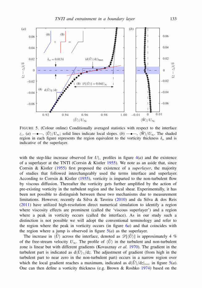
FIGURE 5. (Colour online) Conditionally averaged statistics with respect to the interfacezi. (a) —•—, 〈U〉/U∞; solid lines indicate local slopes. (b) —•—, 〈W〉/U∞. The shadedregion in each figure represents the region equivalent to the vorticity thickness δω and isindicative of the superlayer.

with the step-like increase observed for U|i profiles in figure 4(a) and the existenceof a superlayer at the TNTI (Corrsin & Kistler 1955). We note as an aside that, sinceCorrsin & Kistler (1955) first proposed the existence of a superlayer, the majorityof studies that followed interchangeably used the terms interface and superlayer.According to Corrsin & Kistler (1955), vorticity is imparted to the non-turbulent flowby viscous diffusion. Thereafter the vorticity gets further amplified by the action ofpre-existing vorticity in the turbulent region and the local shear. Experimentally, it hasbeen not possible to distinguish between these two mechanisms due to measurementlimitations. However, recently da Silva & Taveira (2010) and da Silva & dos Reis(2011) have utilized high-resolution direct numerical simulation to identify a regionwhere viscosity effects are prominent (called the ‘viscous superlayer’) and a regionwhere a peak in vorticity occurs (called the interface). As in our study such adistinction is not possible we will adopt the conventional terminology and refer tothe region where the peak in vorticity occurs (in figure 6a) and that coincides withthe region where a jump is observed in figure 5(a) as the superlayer.

The increase in 〈U〉 across the interface, denoted as D[〈U〉] is approximately 4 %of the free-stream velocity U∞. The profile of 〈U〉 in the turbulent and non-turbulentzone is linear but with different gradients (Kovasznay et al. 1970). The gradient in theturbulent part is indicated as d〈U〉T/dz. The adjustment of gradient (from high in theturbulent part to near zero in the non-turbulent part) occurs in a narrow region overwhich the local gradient reaches a maximum, indicated as d〈U〉/dz|max in figure 5(a).One can then define a vorticity thickness (e.g. Brown & Roshko 1974) based on the


0.7

0.9

–2

–1

0

1

2

0.5

1.10 0.2 0.4

1.3 1.6 1.9 2.2 2.5

(a () b () c)

–1

0

1

–20 1 2 0 0.1 0.2 0.4 0.6 0.8 1.03 4

2

FIGURE 6. (Colour online) Conditionally averaged statistics with respect to the interfacezi. (a) —•—, spanwise vorticity 〈Ωy〉 · δ/uτ ; solid (shown in red online) line, (5.5); dashed(black) line, d〈U〉/dz. (b) —•—, Reynolds shear stress 〈−u′w′〉/u2

τ ; dashed line is thelocally linear behaviour. Insert on (b): solid (shown in blue online) line, Reynolds shearstress in the identified non-turbulent zones only; solid (black) line, Reynolds shear stress−uw. (c) —O— (shown in blue online), r.m.s. of the spanwise vorticity 〈ω′yω′y〉1/2 (topabscissa); —— (black), r.m.s. of the streamwise fluctuations 〈u′u′〉1/2; —— (shownin red online), r.m.s. of wall-normal fluctuations 〈w′w′〉1/2 (bottom abscissa). The shadedregion in each figure represents the region equivalent to the vorticity thickness δω and isindicative of the superlayer.

measured change in 〈U〉 and its local gradient as

δω ≡ D[〈U〉]d〈U〉

dz

∣∣∣∣max

. (5.1)

In the present study we find that δω = 0.013δ or δ+ω = 195 for our Reynolds numberand δω is shown as the shaded region in figure 5. In our study the finite interrogationwindow size is likely to have a filtering effect on the resolved velocity gradient acrossthe superlayer and the subsequent estimate of δω. The experimental value of δω is thusconsidered as an upper bound for the superlayer thickness at this particular Reynoldsnumber.

It is seen that the most significant change in 〈U〉 occurs over the region equivalentto the vorticity thickness and hence δω is considered as the superlayer width. Asimilar steep rise in streamwise momentum has been previously observed by Hedley& Keffer (1974a) who found a sharp increase in derivatives of velocity componentsacross the TNTI using conditional sampling. Chen & Blackwelder (1978) usedtemperature as a passive contaminant to show that steep variation in velocities in theouter part are associated with temperature fronts that essentially are ‘backs’ of theturbulent bulges. More recently, Semin et al. (2011) used tomographic PIV data todocument the conditionally averaged profiles of streamwise momentum and spanwisevorticity similar to those in figure 5. Their results do not quantitatively agree withour experiments, and this is attributed to the low Reynolds number in their study(Reτ = 600). The sudden change in streamwise momentum is often referred to as a


‘jump’ in velocity across the interface and has been found in TNTI of wakes and jets(Bisset et al. 2002; Westerweel et al. 2005).

The conditional profile of 〈W〉 lacks a similar distinct jump across the interface.It is known that across the interface a jump in the tangential velocity componentoccurs (e.g. Bisset et al. 2002; Holzner et al. 2007; Westerweel et al. 2009), whilethe velocity component normal to the local interface is uniform (Reynolds 1972). Theturbulent boundary layer under zero pressure gradient grows gradually (dδ/dx≈ 0.012at Reτ = 14 500, see appendix A) and the growth rate decreases further downstream.Although the instantaneous interface is contorted the average interface is boundedby the slow growth rate of the boundary layer itself, i.e. dZi/dx ≈ (Zi/δ) · (dδ/dx)(Zi/δ→ constant, see § 4). Under such conditions the wall-normal velocity W willcontribute the most to the mean velocity normal to the mean interface while thestreamwise velocity U will dominate the mean tangential velocity. The presenceof a jump in the 〈U〉 profile and the relative absence of a jump in 〈W〉 profileis thereby consistent. We find from figure 5(b) that the normal velocity at theinterface 〈Wi〉 = −0.05 m s−1 is negative and consistent with the understanding thatmomentum from the non-turbulent region is being brought into the turbulent regionby entrainment. We can proceed further by making the approximation that the velocitycomponents in a frame of reference on the interface and parallel to the coordinatesx and z are sufficient to study the average statistics about the interface in lieu ofcomponents that are locally tangential and normal to the outline s.

For further observations of the conditional statistics at the interface we normalizethe wall-normal distance relative to the local interface (z–zi) by the vorticity thicknessδω in figure 6. The observed jump in streamwise velocity is accompanied by acorresponding peak in spanwise vorticity in figure 6(a). The theoretical analysis ofReynolds (1972) predicts a discontinuity in mean vorticity across the interface. Thepeak in spanwise vorticity resides within the region indicated by the vorticity thicknessδω. The spanwise vorticity is finite and approximately constant in the turbulent regionand this observation is consistent with the linear slope of 〈U〉 on the turbulent side infigure 5(a). The vorticity magnitude approaches near zero on the non-turbulent side.As one moves along the interface, homogeneity can be assumed in the tangentialdirection due to the slow growth of mean interface location, i.e. ∂( )/∂x→ 0 formean quantities, and the same can be assumed for the conditional averages. Therefore,the mean vorticity within the interface in figure 6(a) can be expressed as

〈Ωy〉 ≈ d〈U〉dz

. (5.2)

This assumption is easily verified by the fact that the wall-normal gradient ofstreamwise velocity in figure 5(a) alone is sufficient to account for the mean vorticitywithin the interface in figure 6(a) (see the dashed line in figure 6a). The behaviourof velocity (and thereby the vorticity) across the TNTI can be modelled as thesuperposition of two components (Bisset et al. 2002; Westerweel et al. 2005): (A) aprofile with linear slope in the turbulent region and zero slope in the non-turbulentregion and (B) a step change in velocity (from being non-zero in the turbulent flowto zero in the non-turbulent flow) in the form of a Heaviside step function H(ξ).This simplified model is depicted in figure 5(a) and can be written as

〈U〉(ξ)=U∞ + d〈U〉Tdξ· ξ [1−H(ξ)]︸︷︷︸

(A)

−D[〈U〉] [1−H(ξ)]︸︷︷︸(B)

. (5.3)


Here we adopt ξ = z− zi for convenience. The above equation can be differentiatedwith respect to ξ to obtain

d〈U〉dξ=D[〈U〉] δ(ξ)+ d〈U〉T

dξ[1−H(ξ)]. (5.4)

Even though mathematically the jump in 〈U〉 is represented across an infinitelysmall region, in reality the viscous effects play a role and the jump occurs over asmall but finite region. Also, in the experimental data there exists a random error inlocating the interface over its finite width for discretely spaced data (it is recalledthat in the present study the distance between adjacent vectors is 50 viscous units).The conditional averages would suffer from this uncertainty and therefore (5.4) isconvolved with a Gaussian kernel (exp[−ξ 2/2/R2]) to account for the ‘smearing’ ofstatistics:

〈Ωy〉 ≈ d〈U〉dξ=D[〈U〉] 1√

2π Rexp

(− ξ 2

2R2

)+ d〈U〉T

dξ

[12− 1

2erf(

ξ√2R

)]. (5.5)

Here ‘erf’ is the error function. Equation (5.5) is in reasonably good agreement withthe measured 〈Ωy〉 with the parameter Ruτ/ν = 75 in figure 6(a) (with measuredD[〈U〉] and d〈U〉T/dξ from figure 5a). The convolution with a Gaussian kernel andthe subsequent agreement with the data implies that the error in determining theinterface is indeed random (a Gaussian process). One cannot deduce the size of thesuperlayer based on the width of such a Gaussian kernel, as it only sets an upperlimit to the actual thickness.

Fluctuating components of U, W and Ωy are found with respect to the conditionalmean profiles in figures 5(a), 5(b) and 6(a), respectively, and referenced to the ziordinate. These are denoted as u′, w′ and ω′y for the streamwise, wall-normal andvorticity fluctuations, respectively. The profiles for Reynolds shear stress and the rootmean square (r.m.s.) of fluctuations are plotted in figure 6(b) and (c), respectively.The conditional Reynolds shear stress at the interface is found to be zero and rapidlyincreases in the turbulent region. Note that the location where 〈−u′w′〉 becomes zerocoincides with the peak in vorticity in figure 6(a). On the non-turbulent side awayfrom the interface the Reynolds shear stress is oppositely signed and varies slowlyto approach a constant value in the fully non-turbulent region. A non-zero value forthe conditional Reynolds shear stress 〈u′w′〉 in the non-turbulent region immediatelynext to the interface is also documented by Bisset et al. (2002) in a wake and byWesterweel et al. (2009) in a jet. This behaviour should not be interpreted as theexistence of non-zero eddy viscosity beyond the TNTI in a boundary layer. In theabsence of vortical motions in the non-turbulent flow the eddy viscosity is zero. Thefinite 〈−u′w′〉 in the non-turbulent region is an artifact of the conditional averagingacross the interface. As we have seen earlier, due to the changing interface heights,the potential streamlines change direction instantaneously. These bulk motions abovethe interface have large-scale variations in streamwise and wall-normal momentumand thus contribute to the non-zero Reynolds shear stress. As a check, we havecalculated the Reynolds shear stress in the laboratory frame of reference at eachwall-normal position by considering only the non-turbulent regions. Thereby theReynolds shear stress obtained within the non-turbulent zones only is plotted versusthe distance from the wall as the solid (shown in blue online) line in the inset infigure 6(b). The calculated Reynolds shear stress in the non-turbulent zones is indeedinsignificant compared to the average Reynolds shear stress −uw in the boundary


layer (solid black line in the inset). Similar observations were made by Hedley &Keffer (1974a) and Jiménez et al. (2010) for boundary layers. Note that in the caseof a turbulent jet/wake the width of the mean flow is defined as the half-width. Thiswould imply that in the laboratory frame of reference a non-zero shear stress existsoutside the jet/wake width, while by definition of δ in the present study no turbulenceand thereby shear stress exists beyond the boundary-layer thickness.

A simplified tangential momentum balance (see equation (3.1c) of Reynolds 1972)relates the change in 〈U〉 across the superlayer to the change in the turbulent shearas

D[〈−u′w′〉] =−〈Wi〉D[〈U〉]. (5.6)

Here D[ ] is a difference operator, D[〈−u′w′〉] and D[〈U〉] are the changes in themean Reynolds shear stress and mean tangential velocity respectively across theinterface. From figure 5(a) and (c), D[〈U〉] = 0.04U∞ and D[〈−u′w′〉] = −0.11u2

τ ,respectively. Therefore, we get

〈Wi〉 =−D[〈−u′w′〉]D[〈U〉] =−

0.0430.80

=−0.053 m s−1. (5.7)

The above estimate of the normal velocity across the interface is in excellentagreement with the directly measured 〈Wi〉 (=−0.05 m s−1). The validity of condition(5.7) has also been experimentally observed by Westerweel et al. (2009) in turbulentjets. The quantitative agreement of (5.5) and (5.6) with the measurements indicatethat we have correctly captured the TNTI dynamics and the approximations regardingthe tangential and normal components of velocity are appropriate.

The r.m.s. of the fluctuating components shown in figure 6(c) also show a rapidincrease in the r.m.s. as one crosses from the non-turbulent region to the turbulentregion. The r.m.s. is non-zero above the interface which should not be interpretedas turbulence. The contribution to the r.m.s. is from the large-scale variations in thepotential streamlines at the edge of the interface as the interface position movesrelative to the wall. Both 〈w′w′〉 and 〈ω′yω′y〉 profiles show antisymmetric behaviouracross the interface with respect to the local magnitude at ξ = 0. The increase in thevariance of the fluctuations is consistent with the behaviour of the mean quantitiesacross the interface and previous observation of TNTI in jets by Westerweel et al.(2009).

It should be noted that (5.5) for vorticity is analogous to the vorticity in an Oseenvortex. Furthermore, in figure 5(a) we observe that the streamwise velocity profileresembles a shear layer, the vorticity has a Gaussian peak behaviour and the shearstress is zero at the interface and oppositely signed on either side. These characteristicsindicate that a certain vortex-like feature or vortex sheet resides within the interface.If the interface is indeed populated with vortices or vortex-like motions, then thecharacteristic length of such motions will represent the scales at which entrainmentoccurs, which shall be the concern in the following sections.

6. An estimate of length scalesIn this section we use two-point correlation as a tool to obtain information about

dominant length scales at the boundary-layer interface. Such analysis follows fromthe work of Westerweel et al. (2005) and Ishihara, Hunt & Kaneda (2012) whocalculated the spatial auto-correlation of conditional velocity along the interface. Asimilar approach is adopted here, although the normal velocity at the interface willbe considered. In the present analysis a local kinetic energy criteria as outlined


(b)

(c)

10–2 10–1 100

(a)

0 0.5 1.0 1.5 2.0 2.5 3.0 3.5 4.0 4.5

0

–1

1

0.2

0.4

0.6

0.8

0

1.0

sn

FIGURE 7. (Colour online) (a) Schematic for calculation of unit vector normal tothe interface. (b) Instantaneous normal velocity at the interface of figure 2(b). (c)Auto-correlation Ru′nu′n of fluctuations at the interface that are relative to the mean of Un.

by (3.1) is applied to distinguish the turbulent from the non-turbulent region. Theturbulent kinetic energy (k) is a scalar quantity. As illustrated in figure 7(a), withinthe turbulent region k> 0, while in the non-turbulent region k≈ 0. The local gradientof kinetic energy (∂k/∂n) at the interface will be normal to the instantaneous interfaceoutline. The unit vector n that is normal to the interface is then calculated as

n=− ∇k|∇k| where ∇ = ∂

∂xex + ∂

∂zez. (6.1)

Thereafter the instantaneous normal velocity (Un) at the interface is calculated usingthe measured streamwise velocity Ui and wall-normal velocity Wi at the interface as

Un = Ui · n= Uinx + Winz. (6.2)

Here, nx and nz are the streamwise and wall-normal components of n, respectively.An example of Un for the interface shown in figure 2(b) is plotted versus thedistance s along the interface in figure 7(b). We have considered the outward normalas positive. Since the interface is contorted and the outward normal often points inthe opposite direction of the free stream, the instantaneous normal velocity fluctuateswithin the approximate bounds of (−U∞, U∞). The sudden and rigourous change inthe direction of Un is largely due to the change in the direction of the local normal(or tangent) of the interface, where the local tangent to the interface can be defined


0.5

0 0.5 1.0 1.5 2.0 2.5 3.0 3.5 4.0

0.6

0.7

0.8

0.5

0.6

0.7

0.8

0

0.2

0.4

0.6

0.8

1.0

(a)

(b)

(c)

10–2 10–1 100

0.2 0.4 0.6 0.8 1.0 1.2 1.4 1.6 1.8 2.00

FIGURE 8. (Colour online) (a) Local interface height zi as a function of the streamwisedistance x. (b) Local interface height zi as a function of the distance s along the interface.(c) Auto-correlation of zi(s).

as dzi/ds (see figure 8b). One can then think of the rapid fluctuations in Un a resultof the small-scale contortions in the interface. If the interface lacked such small-scalefeatures the variation of the normal velocity at the interface would be much smoother.Alternately the small-scale contortions could be characterized by examining thedirection vector n, however, we utilize Un here as it is also a relevant quantity tocalculate the average mass-flux in a boundary layer at a particular Reynolds number(equation (7.12)).

The variation of normal velocity at the interface exhibits characteristics similarto a turbulent signal. It is obvious that the Un fluctuations have a high-frequency(small wavelength) component. To characterize the associated length scale we obtainthe auto-correlation of velocity fluctuations u′n that are normal to the interface andrelative to the mean of Un, i.e. u′n = Un − 〈Un〉. The auto-correlation is calculatedfor all vector fields and its average is plotted in figure 7(c) versus the shift 1s ofdistance along the interface. The auto-correlation Ru′nu′n shows a clear presence ofsmall-scale features consistent with observed variation in Un. In § 4 we have notedthat the interface length is approximately three times longer than the streamwise


distance. Thereby, a characteristic length scale along the interface (λs) and thestreamwise length scale (λx) would be also bounded by this proportionality. Withthat in consideration, figure 7(c) provides an estimate of length scale Λ+x ≈ 290 asthe wavelength corresponding to the peak in premultiplied spectra that is obtainedas the cosine transform of the auto-correlation. This estimate points to an inherentsmall-scale process and is of same the order of magnitude as the Taylor microscale(λ+T ≈ 80–300 in the outer region at this particular Reynolds number). Phillips (1972)suggested that the microconvolutions of the interface are of the same scale as theinterface thickness. We find support for this in the fact that the length scale derivedfrom the normal velocity fluctuations over the microconvolutions in our data is of thesame order as the interface thickness inferred as the vorticity thickness. Our analysiswhich is based on the normal velocity at the interface is consistent with the two-pointcorrelation analysis of Westerweel et al. (2005) based on the axial velocity, who alsoconcluded that integral length scales derived from the velocity information at theinterface is close to the Taylor microscale.

The fluctuating characteristic of instantaneous Un at the interface is not apparentwhen the flow field is examined visually (for example in figure 2). Visual examinationof the interface over the velocity field more strikingly gives an impression of itsorganization, i.e. the presence of small-scale contortions over large-scale bulges andvalleys. It then follows that characterizing the large-scale behaviour of the interfacewould point to the length scale that governs this organization. A straightforward wayis to observe the change in the interface height zi that typically fluctuates betweenδ/3 to δ with streamwise distance x. An example of the local interface height forthe velocity field corresponding to figure 2(b) is shown in figure 8(a). The interfaceoutline shows distinct large-scale variation in its local height with respect to themean interface location (Zi ≈ 2δ/3). However, the interface often turns back on toitself and thus x is not a monotonic variable for zi(x). This difficulty is overcomeby characterizing the interface height with the distance s along the interface, i.e.zi(s) as shown in figure 8(b). The abscissa in figure 8(b) is now monotonic. Itshould be noted that the horizontal axis in figure 8(a) and (b) are different butplotted on an equivalent scale. The trends of zi(x) are clearly followed by zi(s)at a proportional distance. For example, the sudden dip in zi(x) (near x/δ ≈ 1.6)is accompanied by a similar dip in zi(s) near s/δ ≈ 3.25. Similarly, the big bulgebetween x/δ≈ 0.5 and x/δ≈ 1.3 in figure 8(a) is also seen for zi(s) at a proportionalscale. The important aspect of figure 8(a) and (b) is that a single proportionalityfactor between s and x can be used to maintain all of the large-scale features of ziand thereby permitting analysis of zi(s). Here we perform auto-correlation of zi(s).Figure 8(c) plots the auto-correlation Rzizi of the interface height along its distanceobtained as an average from 1250 vector fields. The auto-correlation clearly indicatesa large-scale feature which is expected from the visual examination. A characteristiclength scale Λx/δ ≈ 1.7 is again obtained from peak location in the premultipliedspectra calculated from cosine transform of the auto-correlation in figure 8(c). Incontrast to figure 7(c), the estimate of the integral length scale here is approximatelytwo orders of magnitude higher. Figure 8(c) provides a direct validation of theassumption by Corrsin & Kistler (1955) that the mean interface thickness is muchsmaller than the radii of curvature of the interface. Although Un and zi are notdirectly associated with the instantaneous entrainment rate, the two distinct lengthscales identified with help of these two quantities suggest that the dynamics at the


Non-turbulent

Turbulent

Non-turbulent

Turbulent

(a () b)

FIGURE 9. (Colour online) (a) Turbulent flow bounded by mean boundary-layer thicknessδ. (b) Turbulent flow bounded by mean interface Zi.

interface is likely to be a multiscale phenomena. These aspects will be explored inthe following section, particularly for the mass flux.

7. Mass fluxWe now look at the characteristics of mass flux, i.e. the instantaneous and mean

entrainment across the interface.

7.1. Average mass fluxThe mean turbulent boundary layer can be considered as a combination of anirrotational flow beyond the boundary-layer thickness δ, while the turbulence isconfined below (see figure 9a). The free-stream velocities U∞ and W∞ at theboundary-layer edge contribute to the mean entrainment across the boundary (Head1958). Therefore, the average mass flow rate per unit spanwise depth is

dM = ρ [U∞ dδ −W∞ dx]. (7.1)

The mass flux (rate of mass flow per unit area) is then given as

dMdx=ρ

[U∞

dδdx−W∞

](7.2)

=ρ U∞

[dδdx− dδ∗

dx

], (7.3)

where δ∗ is the displacement thickness and the streamwise growth of δ and δ∗

is evaluated from appendix A using expressions (A 11) and (A 12), respectively.On substituting the experimental parameters we obtain dM/dx = 0.21 kg m−2 s−1

from (7.3). Alternately the mean turbulent boundary layer can be considered as anirrotational flow that resides above the mean interface Zi as shown in figure 9(b).The mean interface Zi gradually grows with downstream x similar to the growth of δ.The entrainment mechanism within the interface would be then responsible for takingin the non-turbulent fluid to keep up with the momentum loss at the wall. The meanvelocities at the interface 〈Ui〉 and 〈Wi〉 contribute to the mean entrainment acrossthe interface. Therefore, the average mass flow rate per unit depth is

dM = ρ [〈Ui〉 dZi − 〈Wi〉 dx]. (7.4)


The mass flux (rate of mass flow per unit area) is

dMdx=ρ

[〈Ui〉dZi

dx− 〈Wi〉

](7.5)

≈ρ[〈Ui〉Zi

δ

dδdx− 〈Wi〉

]. (7.6)

From figure 5, 〈Ui〉/U∞ = 0.97 and 〈Wi〉/U∞ = −0.0025. Substituting Zi/δ = 0.67from § 4 and dδ/dx from (A 11) we get dM/dx= 0.20 kg m−2 s−1 from (7.6). A verygood agreement is obtained between (7.3) and (7.6) indicating that the measurementsare consistent with the theory in appendix A. Equivalence of (7.3) and (7.6) resultsin the following relationship between the mean velocity at the interface and the free-stream velocity:

U∞

[dδdx− dδ∗

dx

]≈[〈Ui〉Zi

δ

dδdx− 〈Wi〉

](7.7)

∴[

U∞ − 〈Ui〉Zi

δ

]dδdx=W∞ − 〈Wi〉. (7.8)

The ratio Zi/δ < 1 and approaches a constant value of approximately 2/3 as notedin § 4. Equation (7.8) outlines approximate relations between the mean velocities atthe interface and the free-stream velocities subject to constraint imposed by mass flux.Note that a similar expression for entrainment velocity exists for turbulent jets (Turner1986). With some manipulation to (7.8) it can be shown that 〈Wi〉< 0 and is O(uτ ).

7.2. Instantaneous mass flux

We have seen that the average interface velocities 〈Ui〉 and 〈Wi〉 give an accurateestimate of the ‘average mass flux’ through (7.6); this is the average entrainmentacross the boundary layer. However, instantaneously the mass flux entrained into theboundary layer via the interface depends on the ‘entrainment velocity’ (say, vE, whichis the difference between the fluid velocity and interface velocity), the density and thesurface area (or in the present case interface line length):

dm= ρ vE · n ds, (7.9)

where ds is the interface line element, and the total mass flux is simply∫

dm. Notethat typically the entrainment velocities are of the order of Kolmogorov velocity scale(Holzner et al. 2007) and extremely difficult to measure directly. However, techniquessuch as high-speed PIV where the time evolution of the interface can be tracked tomeasure vi (interface velocity) with simultaneous measurement of Un may be suitable.To proceed further, it is simpler to consider a coordinate system moving with the free-stream velocity, such that v ≡ u − U∞ and U∞ = (U∞, 0, 0), and in this system theturbulent boundary layer grows outwards in time. Following Philip et al. (2014) andvan Reeuwijk & Holzner (2014), appendix B shows that

dm≈ 2ρνK0

vj Sji ni ds, (7.10)

where Sij is the strain-rate tensor and the quantities are evaluated on the interface.To identify the dominant length scales for mass entrainment, it is convenient to


0.2

0.4

0.6

0.8

0

10

20

30

40

50

60

70

80

0

1.0

102 103 104 105

102 103 104

FIGURE 10. (Colour online) Premultiplied mass spectra: •, dm; , mc. Shaded regionindicates the extent over which the vorticity thickness (δ+ω = 195) extends in s and xco-ordinate system at Reτ = 14 500. Dashed-dotted line (shown in red online) indicatesthe peak in the spectra of mc at λx/δ ≈ 0.85.

consider the two-point correlation of dm along the interface, s, or equivalently thespectra (the Fourier transform of the correlation function, Ψ ). Figure 10 shows infilled symbols the premultiplied spectra (ksΨ ) normalized by viscous scales as afunction of wavelength along s, λs = 2π/ks, averaged over 1250 images. In § 4 wefound that the interface length is on an average three times longer than the unitstreamwise distance, i.e. `s/Lx ≈ 3. Therefore, the equivalent streamwise wavelengthλx = λs/3 is shown on the top axis of figure 10. The peak in the spectra suggeststhe scale at which the entrance of the mass appears most frequently. The peak seemsto be close to the vorticity thickness (δ+ω ) and not far from the Taylors microscale(λ+T ≈ 80 to 300 in the outer part of the boundary layer). The peak corresponds tothe dominant length scale observed for the small-scale mechanisms that resemblenibbling. This is also consistent with observations in turbulent jets by da Silva &Taveira (2010), da Silva & dos Reis (2011) that δω ∼ λT . However, it is noted thatsince the measurements are limited in spatial resolution, the small-scale characteristicof dm in figure 10 should be regarded as a qualitative result emphasizing that thelocal scales are of the order of λT . Accordingly, the precise the numerical values areto be interpreted with caution.

To understand the large-scale entrainment mechanism we suggest considering thetotal or the cumulative mass entrained up to a particular distance s:

mc(s)=∫

dm≈ 2ρνK0

∫ s′=s

s′=0vj Sji ni ds′. (7.11)

The rate of mass entrained between two points s1 and s2 along the interface is simplymc(s2) − mc(s1). To characterize this difference in mc(s), we turn to the analogous


structure function of velocity and the way it is used to characterize the dominantsize of eddies (Davidson 2004). To this end we consider the second-order structurefunction of mc(s), 〈1mc〉2(r)≡〈(mc(s+ r)− mc(s))2〉. Since the second-order structurefunction is algebraically related to the auto-correlation, to understand the dominantlength scales in cumulative mass flux it is sufficient to look at the spectra of thefunction mc(s). Figure 10 also shows in empty symbols the premultiplied spectra ofthe cumulative mass flux (ksΨc) normalized by viscous scales, the peak of whichoccurs at λx/δ≈ 0.85. Therefore, motions of O(δ) cause the interface to be contortedand have large-scale indentations, which are responsible for organizing the small-scalenibbling phenomena over the interface. At the Reynolds number considered these scaleestimates clearly demonstrate a wide separation of length scales that are present in theentrainment process.

Note that for the present case the total mass flux was calculated by two methodsemploying the average boundary-layer properties (cf. (7.3)) and the conditional profilesat the TNTI (cf. (7.6)). Ideally we should be able to calculate the total mass flux from(7.11); however, this turns out to be underestimated due to the resolution of the PIVdata (see Philip et al. 2014 for a fuller discussion). Nonetheless, since our averageinterface is stationary (i.e. in the laboratory frame of reference the interface is steadyon an average), the interface velocity on an average is zero, and we can estimate thetotal mass flux (per unit length) by ensemble averaging:

ρ

`

∫ `s

0Un ds, (7.12)

where Un is the velocity normal to the interface, and `s is the total length of theinterface for each image. The ensemble average of mass flux from 1250 images is0.22 kg m−2 s−1. This estimate of average mass flux is in acceptable agreement withthose obtained from (7.3) and (7.6), which are 0.21 and 0.20 kg m−2 s−1, respectively.

8. Summary and conclusionsUtilizing a unique experimental set-up and the HRNBLWT at University of

Melbourne, we have documented the properties of the TNTI of a turbulent boundarylayer at a relatively high Reynolds number. The Kármán number (Reτ = 14 500) ofthe present experiments ensure that there is sufficient scale separation between theviscous scales (ν/uτ ) and the large scales of the flow of O(δ). The multicameraset-up achieves the magnification required to measure the smallest relevant scales(∼6η) while still able to measure structures as long as 2δ. This criteria is importantto study any boundary-layer phenomena that has multiscale dynamics, entrainmentbeing one of them. In comparison with previous experiments at similar high Reynoldsnumbers, the data acquired here provides a wealth of information over a large field ofview with acceptable resolution for both large and small scales. A new approach basedon the local kinetic energy is introduced to identify the TNTI. This approach and thecriteria adopted detects the turbulent and non-turbulent zones in a two-dimensionalvelocity field effectively. The consistency of statistics validate the approach. Asthe kinetic energy criteria is based on velocity, it can be adopted for differentmeasurement techniques and thereby one does not have to rely on passive markersto detect the TNTI. We have shown this for the hotwire data from the same facilityand the collapse of intermittency profiles indicate a Reynolds number invariance overReτ = 2700–22 000. The mean location of the interface (Zi) is at 2δ/3 while thestandard deviation of its spread is δ/9 approximately.


The two-dimensional interface outline is highly contorted and shows identifiablevariations on both large and small scales. It has been previously shown that theTNTI exhibits fractal characteristics. However, here we have evidenced this fractalcharacteristic in a high-Reynolds-number turbulent boundary layer using only velocitymeasurements, in agreement with past observations. Adhering to its fractal nature, theinterface outline also has a significantly longer length per unit streamwise distance.It is concluded that the fractal geometry increases the effective surface area ofthe turbulent flow that is exposed to the non-turbulent free stream and thereby thesmall-scale nibbling mechanism becomes consequential to the net entrainment atsmaller scales.

Conditional analysis at the interface shows that there is a bulk motion associatedwith large variations in the local interface height, i.e. the potential flow adjuststo the instantaneous thickness of the turbulent flow. The local interface height spanstwo-thirds of the upper boundary layer and appears in the form of large bulges/valleys.The conditional averages shown in figure 5 with interface height as a reference clearlyestablish the presence of a superlayer, first proposed by Corrsin & Kistler (1955),in a turbulent boundary layer. The superlayer is characterized by a shear-layer-likeprofile for the streamwise momentum. Also a discontinuity in the spanwise vorticityand a sudden rise in the Reynolds shear stress on the turbulent side is observedat the interface. The width of the interface layer is deduced as 195 viscous units,equivalent to the wall-normal distance over which the jump in streamwise velocity anddiscontinuity in spanwise vorticity occurs. The examination of the superlayer jumpcondition of Reynolds (1972) over this width shows good agreement between theexperiment and theory. Similar characteristics of the superlayer have been observedWesterweel et al. (2005) in jets and Bisset et al. (2002) in wakes.

Figures 3(c) and (d) point to the fractal nature of the interface and sets the stageto examine the dynamics at the interface in a multiscale sense. It suggests that thelength scales on the either extremes of the data in figure 3(c), where the fractalcharacteristic fails to appear, may correspond to two different mechanisms. These twomechanism occur simultaneously however with different outcomes as shown in § 7.It is noted that the fractal nature of scales that are O(δ) is debatable in the absenceof converged statistics. We have examined the dominant length scales at the interfaceand those are that important to the entrainment. The auto-correlation of the normalvelocity at the interface reveals a characteristic scale that is much smaller than theboundary-layer thickness δ. Since the small-scale contortions of the interface geometrydictate the direction of the normal vector (and, thus, the direction and magnitude ofUn), the length scale from the auto-correlation is the order of the scale of thecontortion. On the other hand, the large-scale organization of the interface is revealedby considering the auto-correlation of the local interface height along the interfacelength s. The large-scale organization of the interface in the form of appearanceof bulges and valleys can be either an outcome of local instability at the interface(Townsend 1966) or motions triggered by the near-wall turbulence (Kovasznay 1970).In either case a large-scale bulge/valley influences the flow in the turbulent and thenon-turbulent region in its vicinity (see figure 4c). The large-scale behaviour of theinterface height is of O(δ) and points to the upper extent of motions that influencesthe TNTI dynamics in boundary layers. Further in this study a novel approach ofexamining the mass flux is presented. The average mass flux (mean entrainment)is calculated from the classical boundary-layer growth equation and found to be inexcellent agreement with a newly formulated growth equation of the mean interfacethat consists of the conditional velocity statistics. We further demonstrate that the


instantaneous mass flux over an interface outline has a high-frequency behaviour.This high-frequency behaviour is indicative of small-eddy motions residing in thesuperlayer and resembles nibbling. The cumulative mass flux on the other hand isfound to account for bulk entrainment over the large-scale bulges/valleys of theinterface. It is found that the small-scale phenomenon has an approximate streamwiseextent that is of the same order as the Taylor microscale in the flow. This observationis in agreement with the previous studies made in jets (Westerweel et al. 2009; daSilva & Taveira 2010) and wakes (Bisset et al. 2002). As remarked by da Silva &dos Reis (2011) such TNTI behaviour is a characteristic of flows with mean shear.The small-scale processes of entrainment appear to be statistically independent ofthe large-scale motions that convolute the interface (Phillips 1972). This estimate isalso consistent with the determined width of the superlayer within which spanwisevorticity is concentrated in the form of nibbling motions. The large-scales over whichsignificant non-turbulent momentum is entrained are found to be O(δ). This estimateis of the scale on which the bulges/valleys are organized. We have seen that both thelarge contortions and small wrinkles in the interface outline contribute towards theincreased surface area of a two-dimensional interface. The instantaneous entrainmentrate is enhanced by the abundance of small scales residing on the two-dimensionalTNTI. It is inferred that the large scales govern the overall rate of entrainmentand the small-scale eddy motions reside on the large-scale features, organized in amanner to keep the aggregate entrainment consistent with the boundary-layer growth.Subsequently the small-scale motions convert the non-turbulent flow to a turbulentstate by vorticity transfer through diffusion.

AcknowledgementsThe authors wish to acknowledge the financial support of the Australian Research

Council. Professor C. Meneveau is thanked for stimulating discussions and helpfulcomments on the instantaneous mass-flux analysis.

Appendix A. Evaluation of x derivative of δ and δ∗

The streamwise evolution of a zero-pressure-gradient turbulent boundary layercan be evaluated by integrating the Kármán integral momentum equation to obtainRex(Reθ):

dθdx= dReθ

dRex= u2

τ

U2∞. (A 1)

This can be applied to establish some preliminary identities and subsequently xderivatives of quantities of interest. We start with the Rotta–Clauser skin–frictionrelation, U+∞(Reδ∗) (Monkewitz, Chauhan & Nagib 2007):

U+∞ =1κ

ln Reδ∗ +C, κ = 0.384, C= 3.3. (A 2)

∴ dU+∞dReδ∗

= 1κReδ∗

. (A 3)

From the definition of the shape factor H,

H = 11− IWW/U+∞

⇒ dHdReδ∗

= dHdU+∞

dU+∞dReδ∗

. (A 4)


For the classical logarithmic theory, IWW =∫∞

0 (U+∞ − U+)2d(z/∆) asymptotes to a

constant very quickly which is evident in the experimental data (Monkewitz et al.2007); i.e. IWW = 7.11:

∴ dHdReδ∗

=−H2 IWW

(U+∞)21

κReδ∗. (A 5)

Further,

H = Reδ∗Reθ

⇒ dHdReδ∗

= 1Reθ− H

Reθ

dReθdReδ∗

. (A 6)

∴ dReδ∗dReθ

= H

1+ H IWW

κ(U+∞)2

. (A 7)

Next, we look at the streamwise development of the Rotta–Clauser thickness∆(=δ∗U∞/uτ ) and arrive at the following useful results:

d∆dx= d(Reδ∗ U+∞)

dRex= dReδ∗

dReθ

dReθdRex

d(Reδ∗ U+∞)dReδ∗

(A 8)

= H

1+ H IWW

κ(U+∞)2

1(U+∞)2

(U+∞ +

1κ

)(A 9)

∴ d∆dx= H (κU+∞ + 1)

H IWW + κ(U+∞)2. (A 10)

In a zero-pressure-gradient turbulent boundary layer the ratio ∆/δ asymptotes to aconstant at high Reynolds numbers (Chauhan et al. 2009). Thereby, dδ/dx can beevaluated as

dδdx= δ+

Reδ∗d∆dx. (A 11)

Utilizing the definition of ∆ we can also write

dδ∗

dx= 1

U+∞

[d∆dx+ ∆

uτ

duτdx

]. (A 12)

The term with x derivative of uτ is expressed as

∆

uτ

duτdx=∆

(− 1

U+∞

dU+∞dx

)(A 13)

=−Reδ∗dReθdRex

dReδ∗dReθ

dU+∞dReδ∗

(A 14)

=−Reδ∗H

1+ H IWW

κ(U+∞)2

1(U+∞)2

1κReδ∗

. (A 15)

∴ ∆

uτ

duτdx=− H

H IWW + κ(U+∞)2. (A 16)

We can now evaluate the streamwise growth rate of δ and δ∗ by utilizing (A 10) and(A 16) in (A 11) and (A 12).


(a () b)

tnelubrut-noNtnelubrut-noN

tnelubruTtnelubruT

FIGURE 11. (Colour online) Turbulent boundary layer in a reference frame where wallis moving at U∞. The non-turbulent control volume CV(x, t) changes with time t. (a) Attime t = to, CV(x, t = to). (b) At time t = t0 + 1t, CV(x, t = to + 1t). The interface isshown to move with a velocity vI .

Appendix B. Turbulent entrainment into a non-turbulent volumeHere we follow the analysis of Philip et al. (2014) where an expression for the

‘entrainment velocity’ (to be defined below) is derived based on an isokinetic energyTNTI. A similar analysis has also been carried out by van Reeuwijk & Holzner (2014),however using an isovorticity TNTI. The purpose of this appendix is to provide aself-contained treatment of the ‘entrainment velocity’ for the sake of completeness,which will be employed to investigate the dominant length scales present during themass entrainment.

We employ a coordinate system moving with the free-stream velocity U∞, such thatthe kinetic energy, K = (1/2)(v · v), where v ≡ u − U∞ and U∞ = (U∞, 0, 0). Theevolution equation for K is

∂K∂t+ ∂

∂xi(viK)= ∂

∂xi

(−vj

pρδij + vj2νSji

)− 2νSji

∂vj

∂xi, (B 1)

where Sij = (1/2)(∂vi/∂xj + ∂vj/∂xi). Now consider the non-turbulent control volume(CV) shown as a shaded region in figure 11 which is changing in time with themoving interface. On integrating (B 1) over a control volume in the non-turbulent (andalmost irrotational, see figure 11) region CV(x, t) and subsequently employing theLeibniz–Reynolds integral rule, one obtains

dKCV

dt=∫

SK(vi − vI i)ni, dS+

∫S

(vj

pρδij − vj2νSji

)ni dS−D. (B 2)

Here, the normal vector n = −∇K/|∇K|K=K0 is pointing into the CV (K0 is thethreshold used for detecting the interface), S(x, t) is the surface enclosing CV , vIis the velocity of the surface or the interface, KCV ≡

∫CV(x,t) K dV , and D is the

dissipation inside CV(x, t). Now, the local entrainment velocity is the difference ofthe interface velocity and the fluid velocity vE ≡ vI − v. As shown in Philip et al.(2014), equation (B 2) reduces to ∫

SI

vE · n dS≈ Φν

K0, (B 3)

where Φν ≡∫

SI2νvjSjini dS, and similarly its two-dimensional equivalent Φ2D

ν can bedefined with i, j= 1, 3 for the present purpose where we have velocity fields on onlytwo-dimensional PIV planes.


REFERENCES

ADRIAN, R. J. 2007 Hairpin vortex organization in wall turbulence. Phys. Fluids 19, 041301.ANAND, R., BOERSMA, B. J. & AGRAWAL, A. 2009 Detection of turbulent/non-turbulent interface

for an axisymmetric turbulent jet: evaluation of known criteria and proposal of a new criterion.Exp. Fluids 47 (6), 995–1007.

ANTONIA, R. A. 1972 Conditionally sampled measurements near the outer edge of a turbulentboundary layer. J. Fluid Mech. 56 (1), 1–18.

BISSET, D. K., HUNT, J. C. R. & ROGERS, M. M. 2002 The turbulent/non-turbulent interfacebounding a far wake. J. Fluid Mech. 451, 383–410.

BROWN, G. L. & ROSHKO, A. 1974 On density effects and large structure in turbulent mixing layers.J. Fluid Mech. 64, 775–816.

CANNON, S., CHAMPAGNE, E. & GLEZER, A. 1993 Observations of large-scale structures in wakesbehind axisymmetric bodies. Exp. Fluids 14, 447–450.

CHAUHAN, K. A., MONKEWITZ, P. A. & NAGIB, H. M. 2009 Criteria for assessing experiments inzero pressure gradient boundary layers. Fluid Dyn. Res. 41, 021404.

CHEN, C.-H. P. & BLACKWELDER, R. F. 1978 Large-scale motion in a turbulent boundary layer: astudy using temperature contamination. J. Fluid Mech. 89, 1–31.

COLES, D. E. & HIRST, E. A. 1968 Computation of turbulent boundary layers. In Proceedings ofAFOSR-IFP Stanford Conference, vol. 2 .

CORRSIN, S. & KISTLER, A. L. 1955 Free-stream boundaries of turbulent flows. Tech. Rep. TN-1244.NACA, Washington, DC.

DA SILVA, C. B. & DOS REIS, R. J. N. 2011 The role of coherent vortices near the turbulent/non-turbulent interface in a planar jet. Phil. Trans. R. Soc. Lond. A Math. Phys. Sci. 369, 738–753.

DA SILVA, C. B. & PEREIRA, J. C. F. 2008 Invariants of the velocity-gradient, rate-of-strain, andrate-of-rotation tensors across the turbulent/nonturbulent interface in jets. Phys. Fluids 20 (5),055101.

DA SILVA, C. B. & TAVEIRA, R. R. 2010 The thickness of the turbulent/nonturbulent interface isequal to the radius of the large vorticity structures near the edge of the shear layer. Phys.Fluids 22, 121702.

DAVIDSON, P. A. 2004 Turbulence: An Introduction for Scientists and Engineers. Oxford UniversityPress.

DE SILVA, C. M., CHAUHAN, K. A., ATKINSON, C. H., BUCHMANN, N. A., HUTCHINS, N.,SORIA, J. & MARUSIC, I. 2012 Implementation of large-scale PIV measurements for wallbounded turbulence at high Reynolds numbers. In Proceedings of 18th Australasian FluidMechanics Conference, 3–7 December, Launceston, Australia.

DE SILVA, C. M., PHILIP, J., CHAUHAN, K., MENEVEAU, C. & MARUSIC, I. 2013 Multiscalegeometry and scaling of the turbulent-nonturbulent interface in high Reynolds number boundarylayers. Phys. Rev. Lett. 111, 044501.

FACKRELL, J. E. & ROBINS, A. G. 1982 Concentration fluctuations and fluxes in plumes from pointsources in a turbulent boundary layer. J. Fluid Mech. 117, 1–26.

FIEDLER, H. & HEAD, M. R. 1966 Intermittency measurements in the turbulent boundary layer.J. Fluid Mech. 25, 719–735.

HANCOCK, P. E. & BRADSHAW, P. 1989 Turbulence structure of a boundary layer beneath a turbulentfree stream. J. Fluid Mech. 205, 45–76.

HART, D. P. 2000 PIV error correction. Exp. Fluids 29 (1), 13–22.HEAD, M. R. 1958 Entrainment in the turbulent boundary layer. Aero. Res. Counc. Rep 3152.HEDLEY, T. B. & KEFFER, J. F. 1974a Some turbulent/non-turbulent properties of the outer

intermittent region of a boundary layer. J. Fluid Mech. 64, 645–678.HEDLEY, T. B. & KEFFER, J. F. 1974b Turbulent/non-turbulent decisions in an intermittent flow.

J. Fluid Mech. 64, 625–644.HOLZNER, M., LIBERZON, A., NIKITIN, N., KINZELBACH, W. & TSINOBER, A. 2007 Small-scale

aspects of flows in proximity of the turbulent/nonturbulent interface. Phys. Fluids 19, 071702.HOLZNER, M. & LÜTHI, B. 2011 Laminar superlayer at the turbulence boundary. Phys. Rev. Lett.

106, 134503.


HUNT, J. C. R. 1994 Atmospheric jets and plumes. In Recent Research Advances in the FluidMechanics of Turbulent Jets and Plumes (ed. P. Davies & M. J. V. Neves), pp. 309–334.Kluwer.

HUNT, J. C. R., ROTTMAN, J. W. & BRITTER, R. E. 1984 Some physical processes involved inthe dispersion of dense gases. In Proceedings of IUTAM Symposium ‘Atmospheric Dispersionof Heavy Gases and Small Particles’ (ed. G. Ooms & H. Tennekes), pp. 361–395. Springer.

HUTCHINS, N., NICKELS, T. B., MARUSIC, I. & CHONG, M. S. 2009 Hot-wire spatial resolutionissues in wall-bounded turbulence. J. Fluid Mech. 635, 103–136.

ISHIHARA, T., HUNT, J. C. R. & KANEDA, Y. 2012 Intense dissipative mechanisms of strong thinshear layers in high Reynolds number turbulence. Bull. Am. Phys. Soc. 57 (17), A23.00004.

JIMÉNEZ, J., HOYAS, S., SIMENS, M. P. & MIZUNO, Y. 2010 Turbulent boundary layers and channelsat moderate Reynolds number. J. Fluid Mech. 657, 335–360.

KHASHEHCHI, M., OOI, A., SORIA, J. & MARUSIC, I. 2013 Evolution of the turbulent/non-turbulentinterface of an axisymmetric turbulent jet. Exp. Fluids 54 (1), 1–12.

KOVASZNAY, L. S. G. 1967 Structure of the turbulent boundary layer. Phys. Fluids Suppl. 10,S25–S30.

KOVASZNAY, L. S. G. 1970 The turbulent boundary layer. Annu. Rev. Fluid Mech. 2, 95–112.KOVASZNAY, L. S. G., KIBENS, V. & BLACKWELDER, R. F. 1970 Large-scale motion in the

intermittent region of a turbulent boundary layer. J. Fluid Mech. 41, 283–325.KULANDAIVELU, V. 2012 Evolution of zero pressure gradient turbulent boundary layers from different

initial conditions. PhD thesis, The University of Melbourne, Melbourne, Australia.MARUSIC, I. & KUNKEL, G. J. 2003 Streamwise turbulence intensity formulation for flat-plate

boundary layers. Phys. Fluids 15, 2461–2464.MATHEW, J. & BASU, A. J. 2002 Some characteristics of entrainment at a cylindrical turbulence

boundary. Phys. Fluids 14, 2065–2072.MENEVEAU, C. & SREENIVASAN, K. R. 1990 Interface dimension in intermittent turbulence. Phys.

Rev. A 41 (4), 2246–2248.MONKEWITZ, P. A., CHAUHAN, K. A. & NAGIB, H. M. 2007 Self-consistent high-Reynolds-number

asymptotics for zero-pressure-gradient turbulent boundary layers. Phys. Fluids 19, 115101.NYCHAS, S. G., HERSHEY, H. C. & BRODKEY, R. S. 1973 A visual study of turbulent shear flow.

J. Fluid Mech. 61, 513–540.PAIZIS, S. T. & SCHWARZ, W. H. 1974 An investigation of the topography and motion of the

turbulent interface. J. Fluid Mech. 63 (2), 315–343.PHILIP, J. & MARUSIC, I. 2012 Large-scale eddies and their role in entrainment in turbulent jets

and wakes. Phys. Fluids 24, 055108.PHILIP, J., MENEVEAU, C., DE SILVA, C. M. & MARUSIC, I. 2014 Multiscale analysis of fluxes at

the turbulent/non-turbulent interface in high Reynolds number boundary layers. Phys. Fluids26, 015105.

PHILLIPS, O. M. 1972 The entrainment interface. J. Fluid Mech. 51, 97–118.PRASAD, R. R. & SREENIVASAN, K. R. 1989 Scalar interfaces in digital images of turbulent flows.

Exp. Fluids 7 (4), 259–264.REYNOLDS, W. C. 1972 Large-scale instabilities of turbulent wakes. J. Fluid Mech. 54, 481–488.SANDHAM, N. D., MUNGAL, M. G., BROADWELL, J. E. & REYNOLDS, W. C. 1988 Scalar

entrainment in the mixing layer. In Proceedings of the Summer Program, CTR - Stanford pp.69–76.

SCHNEIDER, W. 1981 Flow induced by jets and plumes. J. Fluid Mech. 108 (1), 55–65.SEMIN, N. V., GOLUB, V. V., ELSINGA, G. E. & WESTERWEEL, J. 2011 Laminar superlayer in a

turbulent boundary layer. Tech. Phys. Lett. 37 (12), 1154–1157.SREENIVASAN, K. R. 1991 Fractals and multifractals in fluid turbulence. Annu. Rev. Fluid Mech.

23 (1), 539–604.SREENIVASAN, K. R. & MENEVEAU, C. 1986 The fractal facets of turbulence. J. Fluid Mech. 173,

357–386.SREENIVASAN, K. R., RAMSHANKAR, R. & MENEVEAU, C. 1989 Mixing, entrainment and fractal

dimensions of surfaces in turbulent flows. Phil. Trans. R. Soc. Lond. A Math. Phys. Sci. 421(1860), 79–108.


TAYLOR, G. I. 1921 Diffusion by continuous movements. Proc. Lond. Math. Soc. 20, 196–211.TAYLOR, G. I. 1958 Flow induced by jets. J. Aerosp. Sci. 25, 464–465.THOMPSON, B. G. J. 1964 A critical review of existing methods of calculating the turbulent boundary

layer. Aero. Res. Counc. Rep 3447.TOWNSEND, A. A. 1966 The mechanism of entrainment in free turbulent flows. J. Fluid Mech. 26,

689–715.TOWNSEND, A. A. 1976 The Structure of Turbulent Shear Flow. Cambridge University Press.TURNER, J. S. 1986 Turbulent entrainment: the development of the entrainment assumption, and its

application to geophysical flows. J. Fluid Mech. 173, 431–471.VAN REEUWIJK, M. & HOLZNER, M. 2014 The turbulence boundary of a temporal jet.. J. Fluid

Mech. 739, 254–275.WESTERWEEL, J., FUKUSHIMA, C., PEDERSEN, J. M. & HUNT, J. C. R. 2005 Mechanics of the

turbulent-nonturbulent interface of a jet. Phys. Rev. Lett. 95, 174501.WESTERWEEL, J., FUKUSHIMA, C., PEDERSEN, J. M. & HUNT, J. C. R. 2009 Momentum and

scalar transport at the turbulent/non-turbulent interface of a jet. J. Fluid Mech. 631, 199–230.

Documents

J. Fluid Mech. (2014), . 742, doi:10.1017/jfm.2013.641 … · Nychas, Hershey & Brodkey (1973) by visualization showed the occurrence of transverse vortices and suggested that they