Liquidity in the Pricing of Syndicated Loans*

Anurag Gupta1

Ajai K. Singh2

Allan A. Zebedee3

April 2007 Forthcoming, Journal of Financial Markets

1Department of Banking and Finance, Weatherhead School of Management, Case Western Reserve University, 10900 Euclid Avenue, Cleveland, Ohio 44106-7235. Ph: (216) 368-2938, Fax: (216) 368-6249, E-mail: anurag@case.edu. 2Department of Banking and Finance, Weatherhead School of Management, Case Western Reserve University, 10900 Euclid Avenue, Cleveland, Ohio 44106-7235. Ph: (216) 368-0802, Fax: (216) 368-6249, E-mail: ajai.singh@case.edu. 3Department of Economics and Financial Studies, College of Business, Clarkson University, PO Box 5790, Potsdam, NY 13699-5790 Ph: (619) 846-0885, E-mail: azebedee@clarkson.edu. * We thank Allen Berger, Victoria Ivashina, Mitchell Petersen, N. R. Prabhala, Manju Puri, Anthony Saunders, Duane Seppi, S. Viswanathan, the editor Avanidhar Subrahmanyam, an anonymous referee, and the seminar participants at the NBER market microstructure conference and the 2007 AFA meetings for helpful discussions and comments on earlier drafts. We also thank Loan Pricing Corporation and Loan Syndications and Trading Association for providing us the data for this study. We remain responsible for all errors.

Liquidity in the Pricing of Syndicated Loans

ABSTRACT

We examine whether banks price expected liquidity in U.S. syndicated term loans. Using extensive data we show that loans with higher expected liquidity have significantly lower spreads at origination, controlling for other determinants of loan spreads such as borrower, loan, syndicate and macroeconomic variables. A matched sample analysis confirms our results. We estimate that the pricing of expected liquidity results in annual savings of over $1.6 billion to the borrowers, in our sample alone. For the first time in the literature, we identify what influences the decision of financial intermediaries to make secondary markets for an asset, and the consequent pricing impact of this decision in the primary market.

JEL Classification: G12, G21, G32 Keywords: Syndicated loans, loan secondary market, loan pricing, liquidity, loan trading.

1

“… many credit approvals at banks today take into consideration the estimated level of liquidity of the facilities being considered. Liquidity, in this sense, is the relative ease (or lack thereof) of transferability. Factors considered in the liquidity assessment include legal restrictions, availability of potential buyers and, of course, potential discounts.” (PNC Capital Markets Report, PNC Bank, November 2003)

1. Introduction

Syndicated loans represent credit granted by a group of banks or other financial institutions

to a borrower. The originating institutions traditionally sell portions of some of their loans to

other banks and financial institutions via individually negotiated deals, for a variety of

reasons that are outlined in Pennacchi (1988), Gorton and Pennacchi (1995), Haubrich and

Thomson (1996), Dahiya, Puri and Saunders (2003), and others. However, over the last

fifteen years, an active dealer-driven secondary market has emerged, which has led to these

loans being traded, much like debt or equity securities, on an over-the-counter market. The

growth of this market has provided loan originators with several new advantages. For

example, since it is easier for them to sell off loans, they can now free up capital and increase

their grant of new credit, leveraging their comparative advantage in loan origination

activity, thereby increasing their return on assets and equity (Gorton and Haubrich (1990),

Carlstrom and Samolyk (1995) and Demsetz (2000)). Furthermore, originating loans that can

be sold off easily improves the liquidity of the balance sheets of the originating banks,

reduces their financing frictions, and lowers their cost of capital.1 The loan secondary market

also provides originators with a very effective mechanism for risk diversification

(Cebenoyan and Strahan (2002)).

Since increased liquidity provides the loan originators with clear benefits, the natural

question is whether they pass on some of these benefits to the borrowing firms. If the loan

origination market is competitive, then the originating banks must pass on some of the

liquidity-related cost advantage to the borrowers, by charging lower loan spreads at the time

of origination. In this paper, our primary objective is to examine whether the secondary

market loan liquidity has any impact on the pricing of syndicated term loans in the primary

market. In particular, we examine whether banks price the expected liquidity of a loan into

the loan spread at origination, thus passing on some of the liquidity-related benefits to the

borrowers. By examining this primary question, we also address the related question

1 See Stein (1998), Kashyap and Stein (2000), Holmstrom and Tirole (2000) and Diamond and Rajan (2006) for more on this literature.

2

regarding the ability of the originating institutions to ascertain the expected liquidity of a

loan at the time of origination. Financial institutions can only be expected to systematically

price expected liquidity into the loan spread if they can discern with sufficient accuracy, at

the time of origination, the probability that the loan will be liquid in the secondary market.

The concept that liquidity is priced into financial assets plays an important role in the

pricing of all financial assets. Starting with Amihud and Mendelson (1986), several studies

have documented that more liquid assets trade at higher prices (and lower yields).2

However, these studies focus on the determinants of secondary market liquidity and its

pricing implications in the cross-section. For many assets, liquidity must be analyzed at a

more fundamental level – whether secondary markets are made at all or not. What

determines whether there will be a secondary market for an asset? Does this decision to

make secondary markets have any effect on the pricing of these assets in the primary market?

We raise and answer these important questions, for the first time in the literature, using

evidence from the syndicated loans market. This market is ideally suited for such analysis

since secondary markets are never made for a large fraction of the loans originated in the

primary market.

Our study is also the first to analyze the determinants and the pricing impact of liquidity in

a “private” market, as opposed to the public equity and debt markets. The (private)

syndicated loan market is characterized by a trading friction not found in public debt or

equity markets – most loan sales require the consent of either the borrower or the lead bank,

or both. What makes assets liquid, in the presence of such frictions? What is the resultant

pricing impact, if any, in the primary market? We answer these questions using data from

the secondary loan market.

In the syndicated loan market, it is not axiomatic to expect lower spreads on loans that are

liquid in the secondary market. Potentially, as shown in Pennacchi (1988), loan sales could

raise a moral hazard problem because the financial intermediary could reduce its screening

of loan applicants, syndicate the ‘lemons’ and retain the higher quality loans.3 In fact, Boot

2 These studies include Chordia, Roll, and Subrahmanyam (2000), Pastor and Stambaugh (2003), Acharya and Pedersen (2005), and many others in the U.S. equity markets, as well as Krishnamurthy (2002), Chordia, Sarkar and Subrahmanyam (2005), Longstaff (2004), Longstaff (2005) and others in the Treasury and corporate bond markets. 3 The moral hazard problem can be mitigated (Gorton and Pennacchi (1995)) if the originating institution retains a portion of the loan, or by the use of more restrictive covenants (Drucker and Puri (2007)). In this regard, Sufi (2005) presents empirical evidence that the lead arranger retains a larger proportion of the loans that require greater monitoring.

3

(2000) argues that bank loans are illiquid largely due to their information sensitivity,

consistent with the conclusion provided by Bhattacharya and Thakor (1993), that

asymmetric and proprietary information provide the most fundamental explanation for the

existence of financial intermediaries. In such a context, syndicated loans would largely be

illiquid assets, and the sale of a borrower’s loan would convey negative information about

the borrower, consistent with the empirical evidence in Dahiya, Puri and Saunders (2003).

Nonetheless, this line of reasoning suggests that even if the moral hazard problem is

mitigated, controlling for borrower and loan characteristics such as industry, leverage,

credit risk, maturity, size, restrictive clauses etc., the primary market spreads on the loans

that are liquid should be no lower than the spreads on the illiquid loans.

However, these studies analyze loan sales in the context of privately negotiated deals

whereas the emergence of an active dealer-driven secondary market has significantly

altered the market for loan sales.4 Using recent data, Gande and Saunders (2005) show that

when a borrower’s existing loans trade for the first time in the secondary market, it elicits a

positive stock price response. This is opposite to the empirical evidence on loan sales in

earlier papers. Similarly, Drucker and Puri (2007) show that borrowers benefit from loan

sales via increased access to private debt capital, greater likelihood of obtaining future

loans, as well as greater likelihood of preserving their lending relationships, but these

benefits come at the expense of more restrictive covenants. In fact, Guner (2006) argues that

borrowers dislike the sale of their loans and hence they demand a discount on the loan

spread, since the loan sale forces them to deal with multiple banks if and when they need to

renegotiate. However, Guner’s sample period (1987-1993) is not representative of the loan

secondary market today.

As the existing literature has argued, from the borrower’s perspective, there may be

advantages as well as disadvantages to their loans being sold in the secondary market.

Therefore, the impact of these variables on the loan spread at the time of origination is not

unambiguous. From the lender’s perspective, there appear to be clear benefits to originating

loans that are liquid in the secondary market, which suggests that they should charge lower

spreads on these loans, if the loan primary market is competitive. Using extensive loan-level

4 The demand for loans in the secondary market has grown tremendously, partly from hedge funds, while the incentives for banks to sell loans have changed over the years, due to regulation as well as macroeconomic conditions. In Section 2 of the paper, we provide more details on the reasons for the growth of the secondary loan market.

4

primary and secondary market data, we directly examine the impact of liquidity on loan

spreads in order to resolve this question.

Our results show that banks price the expected liquidity of a loan, at the time of origination,

by charging lower spreads on loans that are more likely to trade in the secondary markets,

controlling for other determinants of loan spreads. This liquidity effect is at the loan level,

and not just at the borrower level, since there are liquid as well as illiquid loans in the

market at the same time for the same borrower. We define liquidity as the ease with which

a loan originator can sell the loan in the secondary market, without the need to discount it.

Therefore, in our paper, liquidity measures the ease of locating a counterparty, and hence,

dealer costs and inventory risk from the perspective of the loan originating institution in the

primary market. These search costs are affected by the demand from potential investors,

which is related to borrower as well as loan characteristics. This is similar to the notion that

different claims issued by the same firm (e.g., common versus preferred stock) may have

different levels of liquidity.

Our empirical specifications control for several alternative explanations for the differences

in loans spreads between liquid and illiquid loans. These include differences in credit risk,

information asymmetry, and opaqueness of the borrowers, as well as differences in lender

and loan characteristics (including restrictive covenants). Our results are consistent across

several different sub-samples of loans and robust to several alternative definitions of

liquidity. The magnitude of this pricing effect is very significant (ranging from 88 to 137

basis points) between the most liquid and the most illiquid loans, controlling for other

determinants of loan spreads. As further robustness, we do a matched sample analysis by

comparing the spreads on liquid loans with those on illiquid loans from the same lender to

the same borrower at the same time (hence almost everything is controlled for in these tests,

including any unobservable private information with the lender), and find a consistent

effect.

Interestingly, we find that loans from higher risk borrowers (speculative grade) are more

liquid than loans from lower risk borrowers (investment grade). This is opposite to the

results consistently reported in the studies from the equity markets (see Stoll (1978), Wahal

(1997), Madhavan (2000) and others), that more volatile stocks are less liquid (higher

inventory costs), and stocks of higher risk firms are less liquid (higher adverse selection

costs). Conventional intuition would suggest that dealers should be less willing to make

markets in loans from higher risk borrowers. Our results, to the contrary, are driven by the

5

higher order flow for loans from risky borrowers that more than offsets the higher costs of

the dealers due to other factors. There is greater investor demand for speculative grade

loans, due to their higher yields as well as their suitability for managing the credit risk of

debt portfolios, that leads to greater order flow for these loans.

Our pricing results are qualitatively similar to those reported in studies on the pricing of

liquidity in equity and bond markets, where more liquid assets are reported to have higher

prices and lower yields. However, our paper links the secondary market liquidity of loans to

their primary market pricing, which is fundamentally different from the existing literature

that links liquidity and pricing within the secondary market.5 To our knowledge, this is the

first paper to document expected liquidity being priced into syndicated loan spreads at the

time of their origination.6

Our results suggest that the primary market for loan syndications is quite competitive

(contrary to the suggestions otherwise, in Ho and Saunders (1981) and Guner (2006)), and

the loan arranger shares at least part of the liquidity-related benefit with the borrowing

firms.7 In the aggregate, we estimate that this pricing of expected liquidity into loan spreads

results in an average annual savings of over $1.6 billion to the borrowing firms, just for our

sample of U.S. syndicated term loans. Excluding the naïve explanation of altruistic motives

on the part of banks, there is no reason, other than competition, for banks to share this cost

advantage with their borrowing clientele. Our results also imply that banks must have the

ability to discern the expected liquidity of a loan at the time of its origination. Absent this

ability, we should not see any systematic pricing of expected liquidity into loan spreads.

Our paper is the first in the literature to develop a model for predicting the liquidity of a

loan at the time of its origination.

The rest of the paper is organized as follows. Section 2 introduces the syndicated loan

secondary market. Section 3 provides an overview of the empirical methodology. Section 4

presents the data used in this paper, along with some descriptive statistics. Section 5 5 Ellul and Pagano (2006) show the link between the underpricing of common stock IPOs and their subsequent liquidity in the aftermarket. However, all IPOs subsequently trade in the secondary market. On the other hand, a majority of loans do not. Therefore, the syndicated loan market provides a novel context for examining this linkage. 6 In a contemporary paper, Moerman (2005) relates loan spreads to the information asymmetry associated with the borrowing firm, as proxied by the bid-ask spread on the firm’s prior loans on the secondary market, which is different from the liquidity effect analyzed in this paper. 7 This effect is similar to what happened in the mortgage markets decades ago, where borrowers have benefited (by way of lower mortgage rates) from the liquidity in home loans due to the emergence of mortgage backed securities.

6

presents the empirical results in two parts. The first part focuses on why some loans trade in

the secondary market and others do not. The second part models the syndicated loan

spreads (over LIBOR) at origination as a function of loan, firm, and syndicate characteristics

and macroeconomic conditions. Section 6 presents additional robustness tests. Section 7

concludes the paper.

2. Syndicated Loans and their Secondary Market

A syndicated loan is a large-scale loan typically structured and placed by a lead arranger or

an agent, who then sells portions of the deal (within the primary market) to a syndicate of

financial entities under the negotiated terms and conditions. These loans (or parts thereof)

may then be subsequently transferred from the primary to the secondary market by

assignment or by participation. When transferred by assignment, the buyer/investor

becomes the lender of record; hence it typically requires borrower consent, and frequently

the consent of the lead bank as well. In the case of transfer by participation, the buyer only

obtains the right to re-payment, while the relationship between borrower and the original

lender remains intact. Participation involves an additional element of risk to the buyer since

they do not have any direct claim on the assets of the borrower in the event of default. Most

of the loan trading is by way of assignment.

In 2005, the total primary market U.S. syndicated loan volume was about $1.5 trillion

according to the Loan Pricing Corporation (LPC). Relative to other financing alternatives

syndicated loans account for approximately one-third of all corporate financing and

represent the largest single financing tool used in corporate America. Figure 1 presents the

mix of syndicated loans originated in the U.S. from the year 2000 onwards. While there has

been modest growth in the primary syndicated loan market, the mix of loans has remained

relatively constant over this period with leveraged loans (defined by LPC as loans with a

credit rating below investment grade or loan spread above 150 bp) representing, on average,

about one-third of all new syndicated loan originations.

In contrast, the secondary market for syndicated loans has grown tremendously over the last

decade. Figure 2 presents the secondary market trading volume in syndicated loans in the

U.S., which has grown from just $8 billion in 1991 to over $176 billion in 2005, reflecting a

compounded annual growth rate of nearly 23% per year over the last 15 years. In addition,

the mix of loans has also changed over this time period. As shown in Figure 2, a part of this

growth is the result of increased trading in distressed loans (traded at prices below 90% of

7

par). This stylized fact has so far been the focus of several studies in the academic literature

on syndicated loan sales.

In particular, the previous literature on loan sales, which includes Pennacchi (1988), James

(1987), Gorton and Pennacchi (1995) and others, has largely advocated that banks have

incentives to sell underperforming credits. In this context, Dahiya, Puri and Saunders (2003)

present empirical evidence that loan sale announcements are followed by negative stock

returns for the borrowers along with higher probabilities of their bankruptcy. However, if

the loans being sold are mostly “lemons”, then rational investors would assume adverse

selection (Akerlof (1970)) and discount these loans below fair value, thereby leading to an

unraveling of this market. Then why has the secondary market for loans grown at such a

high rate, especially during the last decade?

The recent literature on loan sales has tried to address this question. Using more recent data,

Gande and Saunders (2005) document a positive stock price reaction for the borrowers,

including distressed firms, at initial loan sale announcements. They argue that loan trading

provides an alternative source of information about the borrower, which is perceived as

“good news” by their equity investors. From a theoretical perspective, Behr and Lee (2006)

argue that loan sales allow banks to choose its optimal funding mix between sophisticated

(loan) and uninformed (deposit) investors. As a result, in equilibrium, banks will always

have incentives to sell off some of their loans.

Therefore, while the influx of distressed loans is one of the reasons for the tremendous

growth of the secondary market for syndicated loans in recent years, it is not the primary

reason. There are several supply side and demand side reasons why this market has grown

and will continue to grow. On the supply side, banks may sell performing corporate credit

exposures for several reasons. The first reason is portfolio management considerations.

Banks may sell loans to avoid excessive risk concentration to particular obligors or

industries, or to move on to higher return opportunities. The second reason is strategic shifts

in lending strategy. At various points in the economic cycle, banks become hot or cold

towards certain industries, geographic regions, or to commercial lending in general. The

third reason is regulatory capital arbitrage as well as regulatory constraints under the Basel

Accord, which have created incentives for banks to sell some loans while holding the others

in order to boost return on capital. In addition, as pointed out by Carlstrom and Samolyk

(1995), regulatory constraints and information asymmetries create the incentive for banks in

one region to originate and sell loans to banks in other regions that have adequate capital.

8

The fourth reason is extraction of economic rents from loan origination activity. Some banks

(especially larger, high reputation banks) are adept at originating credit exposures due to

their expertise in credit assessment and strong client relationships (similar to the arguments

given in Demsetz (2000)). Since banks are required to maintain regulatory capital, additional

loans on their balance sheet result in diminishing marginal benefits. Therefore, the sale of

their loan portfolio allows them to use their capital base more effectively to support a higher

level of origination activity without experiencing balance sheet growth.

On the demand side, starting from the mid-nineties onwards, nonbank financial institutions

like hedge funds, mutual funds and other funds such as CDOs (Collateralized Debt

Obligations) and CLOs (Collateralized Loan Obligations) have emerged as major buyers of

syndicated loans in the primary and the secondary markets. Syndicated loans are senior,

typically secured, floating interest rate instruments that have stricter covenants than bonds,

and higher recovery rates than other debt securities. The returns on these loans are fairly

uncorrelated with equity returns – as per LPC estimates, the correlation of returns between

loans and the S&P 500 was 0.12 between 1992 and 2002. Since 1992, loans have had positive

returns in every single year, including recession years. The Sharpe ratios for various loan

return indices are between 0.8 and 0.9, compared with between 0.6 and 0.7 for bonds and

about 0.3 for the S&P 500 index. Being floating rate instruments, they are free of duration

risk, which makes them attractive to fixed income fund managers. These stable returns and

high recovery rates even in times of credit crunch have attracted many investors to this

market. This is especially true from the year 2000 onwards, since the equity markets have not

provided attractive returns while traditional fixed income instruments have had high

volatility, thereby forcing investors to look to other asset classes for higher, stable yields.

Loans provide them with risk-return characteristics that are not available through any other

asset class. In addition to these investors, the secondary loan market also allows smaller

banks to acquire exposures to sectors or countries where they may not have the critical size

to originate loans in the primary market. These demand side factors have been the primary

drivers of growth in this market.

The investor base in this market primarily consists of sophisticated institutional investors

with virtually no noise traders. The primary market makers are larger investment and

commercial banks, who provide two-way price quotes and commit capital to take outright

9

positions and create liquidity.8 Institutions actively engaged in primary market loan

origination have an advantage in trading on the secondary market, in part because of their

acquired skills in accessing and understanding loan documentation. In addition, the active

traders in this market consist of other commercial and investment banks, distressed debt

traders, and vulture funds. Some non-financial corporations and large institutional investors

like pension funds and insurance companies have also recently started to trade corporate

loans in the secondary market. The heterogeneity of both the issuers and the investors has

enhanced liquidity in this quickly expanding market.

3. Research Hypotheses and Design

Our primary objective is to examine whether the expected liquidity of a syndicated loan is

priced into its yield spread at the time of origination. We do that by a two-stage modeling

process. In the first stage, we develop a model for predicting the liquidity of a loan at the

time of origination. A loan is defined as liquid if there is an available secondary market for it.

Therefore, liquidity captures the ex ante ease with which a loan originator can sell its loan in

the secondary market. Thus, in our paper, liquidity is a function of dealer cost and inventory

risk from the perspective of the primary market issuer of the asset, rather than from the

secondary market dealer’s perspective. The loan originator is likely to incur lower search

costs in locating a counterparty to sell the loan when there is a secondary market for it, and

perhaps lower transaction costs as well. The probability that there will be a secondary

market for a loan captures these search and transaction costs, and hence the inventory risk

faced by the loan originator. Our first-stage model estimates this probability, which is an

innovation in this paper.

In the second stage, we examine whether, controlling for all the other determinants of loan

spreads, the expected liquidity of the loan has any impact on the loan spread at origination.

Our second stage model draws upon the large literature on the determinants of loan

spreads.9 Our innovation in the second stage is the inclusion of the expected liquidity

variable as a determinant of the loan spread in the primary market, controlling for all other

8 Some of the earlier entrants in this market were BT Alex Brown, Bear Stearns, Citibank and Goldman Sachs. Now there are nearly 35 market makers for secondary market trading of syndicated corporate loans, representing the loan trading desks of virtually every large commercial and investment bank. 9 See, for example, Angbazo, Mei, and Saunders (1998), Casolaro, Focarelli, and Pozzolo (2003), Chen (2005), Coleman, Esho, and Sharpe (2004), Dennis, Nandy, and Sharpe (2000), Harjoto, Mullineaux, and Yi (2006), Hubbard, Kuttner, and Palia (2002), Ivashina (2005), Moerman (2005), Santos and Winton (2005), Strahan (1999), and others.

10

determinants previously examined in the literature. We now proceed with a more formal

description of each stage.

In the first stage, we develop a probit model to estimate the probability that there will be a

secondary market for the loan after origination. This model is conditioned on the

information available at the time of origination of the loan, about the loan, the borrower, the

syndicate, and the macroeconomic environment. The cross-sectional model is estimated for a

sample of n loans (i=1,...,n), as follows,

[ ] iiiiiiiiiiii uXXXXXcXXXXXZ ++++++Φ== ,55,44,33,22,11,5,4,3,2,1 '''''),,,,1(P βββββ (1)

where { } )1,0(~,,,, ,5,4,3,2,1 NXXXXXu iiiiii and

Zi: Indicator variable for loan liquidity, equal to one if the loan is classified as liquid,

X1: Vector of loan characteristics,

X2: Vector of borrower characteristics,

X3: Vector of syndicate characteristics,

X4: Vector of macroeconomic variables,

X5: Vector of instruments.

In estimating equation 1, we use an instrumental variables approach as outlined in

Wooldridge (2002). The instruments are needed to predict the liquidity (after partialing out

any controls) in order to ensure that our second stage model can be identified. The

instruments are chosen as factors that affect the probability that there will be a secondary

market for the loan, but do not directly affect the initial spread charged by the syndicated

group. This implies that the instruments for liquidity must be related to factors that affect the

demand for loans in the secondary market, rather than supply side factors. The supply side

factors affect the decision making process between the lenders and the borrower. Therefore,

they implicitly affect both the liquidity and the yield spread of the loan, and thus cannot be

used as instruments. Only factors that drive the demand for a loan in the secondary market,

excluding any characteristic of the loan agreement between the lenders and the borrower,

can potentially be valid instruments.10 We choose two instruments of liquidity in our

10 The lenders and the borrower have different motivations for making the loan liquid. For the lender, it may be improvement of liquidity, diversification of risk, strategic behavior, etc., as discussed in Section 2. For the borrower it may be benefits of increased access to capital versus potentially negative information conveyed by loan sale. These characteristics are reflected in the terms of the loan agreement (for example, covenants). We include all the terms of the loan agreement available to us as explanatory variables in both stages of the model, since they are likely to affect both the liquidity as well as the yield spread on the loan

11

analysis - one (Bank Tier) reflecting a lender characteristic, the other (Transparency) reflecting

a borrower characteristic.11 In our empirical analysis, we statistically examine the strength

and validity of these instruments.

Our first instrument is bank tier as a proxy of bank reputation. The two variables Tier 1 Bank

and Tier 2 Bank measure the rank of the lead arranger based on its primary market share. Tier

1 Bank is equal to one if the lead bank is amongst the top three lead arrangers in the league

tables for 1998-99 (the two years prior to the start of our sample period), while Tier 2 Bank is

equal to one if the lead bank in between the fourth and the thirtieth rank.12 In a competitive

market like the syndicate loan market, the rank of the lead arranger is not expected to matter

in terms of the initial spread, once the identity of the lead bank has been controlled for

(commercial, investment or universal bank). The lead bank’s reputation could, however,

affect the future liquidity of the loan, since the bank’s reputation serves as an implicit

guarantee when a loan is sold in the secondary market, as argued by Gorton and Haubrich

(1990) and Gorton and Pennacchi (1995). This effect is comparable to the certification effect

detailed in the IPO literature (see, for example, Booth and Smith (1986)). Loans originated by

higher tier lead banks are likely to be easier to sell in the secondary market since the buyers

would be more confident in buying these loans. In addition, the higher tier banks have

stronger relationships with institutional investors, who are the major buyers of syndicated

loans in the secondary market. Therefore, it would be easier for higher tier banks to sell the

loans that they originate.

Our second instrument, Transparency, measures the ease of availability of the financial

statements of the borrower. If the firm’s financial statements are publicly available it is easier

for outside investors to evaluate the firm’s loans as a potential investment. This transparency

will not affect the negotiated spread at origination since the syndicate members already have

detailed access to the firm’s financial statements. Therefore, the public availability of the

financial statements of the borrower are only likely to affect the demand for the loans of that

borrower. This variable is therefore only expected to impact the spread through potential

liquidity effects. The Transparency variable is set equal to one if the firm has had any public

equity or debt issue (including Registered Rule 144A debt issuance to qualified institutional

(and hence, cannot be used as instruments). 11 As further justification for their exclusion in the second stage, the variables chosen as instruments proved to be statistically insignificant in the second-stage loan pricing model discussed below. In addition, our results are not sensitive to the choice of instruments. We re-estimated our model with several different sets of instruments, but our primary results remained unchanged. 12 Our results are robust to alternative classifications of lead bank tiers.

12

investors) prior to the loan origination date, since the financial statements of such firms will

be in the public domain.

We classify loans into liquid and illiquid categories using several alternative definitions to

ensure that our results are not driven by any one particular method of defining loan

liquidity. However, it is important to note that any error in our methods of categorizing

loans into liquid versus illiquid will only bias the entire procedure against us. To the extent

that the dependent variable in the probit model is specified with error, there is a lower

likelihood of the model producing accurate predictions of expected liquidity. This will only

attenuate the coefficient on expected liquidity in the second stage regression.

The fitted values of ),,,,1(P ,5,4,3,2,1 iiiiii XXXXXZ = or ip̂ from equation 1 are then included as

an explanatory variable in a regression model of loan spreads. Since we only analyze term

loans in this paper, we use the “All-in Drawn Spread” (AIS) as the loan spread. The AIS is

the sum of the amount the borrower pays in basis points over LIBOR plus any annual or

facility fees paid to the lender. It is a more complete measure (than just the basis points

spread over LIBOR) of the ongoing costs for the borrower as well as the income for the

lender (or the subsequent buyer of the loan), and is used as the standard measure of loan

spreads in the literature.13

The second stage regression model is as follows:

iiiiii pdYYYYcAIS ˆ.'''' ,44,33,22,11 +++++= αααα (2)

where

Y1: Vector of loan controls,

Y2: Vector of borrower controls,

Y3: Vector of syndicate controls,

Y4: Vector of macroeconomic control variables.

13 Annual or facility fees are fairly uncommon in LIBOR based term loans (they are more prevalent in lines of credit), therefore less than 5% of the term loans in DealScan have this data reported. Our results are robust to the exclusion of the loans with annual or facility fees from our sample. For the rest of the loans, the only measure of yield spread that is available is the AIS, hence the literature uses it as the principal pricing measure in the primary market. In later tests, we also use a relative pricing measure to ensure that our results are robust.

13

The objective of this second stage model is to estimate the impact of expected liquidity on

the loan spread, after controlling for all other variables that could affect the spread. The

coefficient of primary interest is “d”, which should be significantly negative if loan

originators price expected liquidity into loan spreads.14 The negative coefficient on expected

liquidity would imply that liquid loans are originated with lower spreads, ex ante, than

illiquid loans, controlling for other determinants of loan spreads.

This two step approach outlined above presents several advantages. First, it allows us to

condition only on the information available at the time of the loan origination. Our key

variable of interest, liquidity, is only observed after the loan has been issued. The first stage

predicts the probability a loan will be liquid conditional on information available at the time

of syndication of the loan. This predicted probability then enters into the second stage loan

pricing model. The second advantage of the two part model is that it allows the regressors to

have a different effect on the likelihood the loan is available in the secondary market and on

the initial spread charged by the banks in the primary market.

Consistent with prior studies, we include several control variables in the second-stage

regression in order to rule out other possible explanations for our results, such as differences

in credit risk, information asymmetry and opaqueness, lender type, and loan characteristics,

between liquid and illiquid loans. Some of the important control variables are discussed

below.

To address the first alternative hypothesis, we control for differences in credit risk between

liquid and illiquid loans. The primary variable we use is the credit rating of the borrower at

the time of origination of the loan. In addition, we use profitability and leverage variables to

control for any residual differences in credit risk. We also use the firm size and the loan size

as proxies for credit risk. Several prior studies (Bharath, Dahiya, Saunders and Srinivasan

(2006), and Harjoto, Mullineaux and Yi (2006), among others) have used firm size to control

for credit risk, and have shown that loans to larger borrowers carry lower spreads, all else

being equal. A larger loan size is also associated with lower spreads. As shown by Booth

(1992), there may be economies of scale in loan origination and monitoring, leading to lower

spreads for larger loans. In addition, it may be argued that banks would give larger loans

only when they are more certain about the credit quality of the borrower, thereby leading to

14 In estimating the two step procedure we use the instrumental variables approach as outlined by Wooldridge (2002). This approach ensures that the standard errors and test statistics are asymptotically valid.

14

lower spreads, as documented by several prior studies (for example, Bharath et al. (2006)).

We control for covenants and collateral, since, as suggested by Rajan and Winton (1995),

these features are more likely to be present in loans to firms that require more intensive

monitoring, and are therefore associated with higher probabilities of distress. The

relationship between loan maturity and spreads is not that unambiguous. Though Flannery

(1986) indicates that longer maturity loans would have higher credit risk, the empirical

evidence on the impact of loan maturity on spreads has been mixed. We control for the loan

maturity to ensure that any impact of maturity on the loan spread is controlled for.

We control for differences in information asymmetry and opaqueness between the

borrowers of the liquid versus illiquid loans by including variables for firm profitability,

firm size, loan size, credit rating, collateral and covenants. In addition, we control for the

industry of the borrower, since firms in some industries are naturally more opaque than

others. We also examined the impact of other potential control variables related to

information asymmetry and opaqueness, such as R&D intensity, intangible asset ratios, and

whether the borrowing firms had any previous public debt issues. We exclude these

variables from the final empirical model due to their statistical insignificance.

In addition to the variables above, we control for the identity of the lead bank – whether it is

an investment or a commercial bank, since Harjoto et al. (2006) show that investment banks

charge higher spreads than commercial banks. We include the number of lead banks as an

additional control for unobserved borrower risk, since safer loans are easier to syndicate

(Guner (2006)). Finally, we control for several loan characteristics, especially the loan

purpose, since the loan purpose could be associated with differences in loan spreads. This is

especially true for loans originated for “Restructuring” purposes (which includes takeovers,

LBOs, spin-offs and stock buy-back), since they alter the capital structure of the borrowing

firm.

4. Data

The data for this study are obtained from five sources – the DealScan database from Loan

Pricing Corporation (LPC), the mark-to-market pricing service from Loan Syndications and

Trading Association (LSTA), Compustat, DataStream and the Securities Data Corporation

(SDC).

15

The loan origination information is obtained from DealScan, which contains data on over $2

trillion of large corporate and middle market syndicated loans, obtained from SEC filings for

public companies and other sources for private companies. All the loan and lender

characteristics and some borrower characteristics are obtained from DealScan. The rest of the

borrower characteristics are obtained from Compustat. The data on macroeconomic

variables are obtained from DataStream. We obtain prior debt issuance data (both public and

Rule 144A) from SDC.

The categorization of loans based on their liquidity is done using a unique dataset of

secondary market loan price quotes from LSTA. They provide independent secondary

market pricing service on syndicated loans to over 100 institutions that manage over $200

billion in bank loan portfolios. LSTA receives bid and ask price quotes for over 3,000 loans

from nearly 35 dealers on a daily basis, in the late afternoon.15 These price quotes reflect the

market information for the day. As part of the pricing service, they provide the average of all

bids and all asks for loans that have more than 2 bid quotes (about 1,800 out of these 3,000

loans have more than 2 bids). They also provide the number of bid and ask quotes

(separately) for each of these loans, along with other information including loan identifier

(LIN), the name of the borrower, and the type of loan.16 We use these secondary market loan

prices to construct several proxies for the liquidity of the loans in our sample.

The volume of loan trading in the secondary market grew steadily during the 1990s, and by

the year 2000, had crossed $100 billion in annual volume. The coverage of our secondary

market data starts in 1996. However, until November of 1999, the coverage is very sparse

(only about 100 loans in the cross section), and is only available monthly. This is reflective of

the lower level of activity during the growth phase of this market, until the year 2000. We

therefore begin our study with loans originated in the year 2000. From the year 2000

onwards, we have daily price quotes, with the number of loans available in the cross-section

in the secondary market database increasing from about 600 in January 2000 to about 1,500

in March 2005.

15 These dealers include the loan trading desks of most of the big commercial and investment banks in New York, and, as per LPC estimates, account for over 80% of the secondary market trading in syndicated loans. 16 Since there is no common identifier between DealScan and the LSTA pricing data, the loans in the secondary market pricing data must be manually matched with the primary market data in DealScan. Further, these two databases do not have any identifier that is recognized in Compustat, so the matching with Compustat also must also be done manually, to ensure zero errors.

16

Our primary measure of liquidity classifies a loan as being liquid if it is quoted in the

secondary market by at least two dealers at any point during this time span, and the first

quoted bid price is greater than 98 (hence it is a par loan). If the loan is quoted by multiple

dealers, then it is reasonable to assume that it is possible to trade that loan on that day. In

addition, if it is first quoted close to or above par, it implies that the loan does not have to be

discounted to initiate a sale. Therefore, as per our definition, a loan is classified as liquid

only if there is a secondary market for it without the need for a fire sale (i.e. a sale at a

discounted price).17

We examine the syndicated loans originated during the five years 2000-2004, covered by

DealScan. We focus only on U.S. dollar (USD) denominated syndicated term loans to U.S.

borrowers. All other types of loans (primarily revolvers and lines of credit) are excluded

from this study because their pricing function at origination is different from that of term

loans. Revolvers and lines of credit also charge a commitment fee on the undrawn portion of

the credit line. However, the undrawn portion never trades. Since it is impossible to predict

the drawdown schedule of a borrower at origination, the incorporation of expected liquidity

into the drawn spread of a credit line is likely to be much less transparent than that in term

loans. In order to have a relatively homogeneous sample of loans where the loan spread has

a clear interpretation, we restrict our analysis to USD term loans to US firms. Over the

sample period there are 7,912 USD syndicated term loans representing 4,975 unique

borrowers available for the analysis.

In the empirical results, we present six distinct specifications drawing on the available

sample of 7,912 USD term loans. These specifications are labeled A through F throughout

our analysis. The sample sizes vary across the specifications due to the differences in data

availability. The first specification A has a sample size of 1,591 loans. It is the most restrictive

sample requiring no missing data for any variable in the estimation process. Specifications B

and C draw on the same sample of 1,591 loans but incorporate control variables for missing

data. The DealScan database has missing data for many loan characteristics which may or

may not be important determinants of the expected liquidity and/or the origination spread.

For many of these characteristics, the data is only reported if there is data to report,

suggesting that missing data may reflect a zero value. To test this statement, we incorporate

indicator variables for each missing field to determine if the missing value is in fact a zero

value. A number of these missing indicator variables do confirm that the missing data is not

17 Our results are robust to defining a loan as liquid even if its first quoted bid price is below 98.

17

important in the models. However, in some cases the estimated parameters for the indicator

variables for the missing fields are statistically different from zero. We retain all missing

indicator variables in the model to control for missing data but do not report these results for

the sake of brevity. These results are available directly from the authors.

In addition, there are multiple data sources for some of our firm specific controls. For

example, credit ratings are available from both DealScan and Compustat. Specifications A, B

and C rely on credit ratings from the Compustat database. The credit rating data are

extracted from Compustat for the fiscal year prior to the loan origination fiscal year.

However, specifications D and E rely on DealScan for credit rating data. In total,

Specification D includes 1,657 loans.

In addition to relying on Compustat for credit rating data, other borrower characteristics

such as sales, R&D expenses to sales, long-term debt, intangible assets to total assets, etc. are

also drawn from Compustat. These data are also populated by a number of missing values

for the loans identified from the DealScan database. By dropping the non-credit rating

borrower characteristics from the empirical specification the sample size increases to 2,791

loans. These results are labeled as Specification E.

Finally, Specification F uses the full sample of 7,912 loans identified from the DealScan

database. All the data used in estimating this model are drawn from the DealScan database.

Where appropriate, controls for missing data are incorporated into the model but other

variables such as credit rating data are excluded from the specification to maximize the

sample available for the analysis.

Table I presents descriptive statistics of the variables across the different samples of loans for

each of the models in our paper. The definition of these variables is provided in the

Appendix. The table presents the mean of the variables across each sub-sample. The

liquidity variable in this table is based on our primary definition of liquidity, as per which a

loan is classified as a liquid loan if on any day after origination there is a price quote for that

loan in our secondary market database, and its first quoted bid price is greater than 98 (par

loan).18 Out of the full sample of 7,912 loans, about 14.9% of the loans are classified as liquid

loans using this definition. These liquid loans represent 736 unique borrowers. In our

18 Note that we only have data for loans that have at least 2 bids, so loans for which only one dealer posted a bid or an ask price are categorized as illiquid.

18

robustness tests, we consider alternative definitions of liquidity as well to check if our results

are sensitive to the definition used for liquidity.

Our full sample of 7,912 loans consists of facilities with a total principal of $1.22 trillion,

covering a significant percentage of the total volume of USD syndicated term loans

originated during 2000-2004. Even our most restrictive sample, Specification A, includes

loans with a total principal of $535 billion dollars. The average size of each loan is about $155

million, with more than 50% of the facilities between $100 million and $500 million. The

average maturity of these loans is about four and a half years. Many of these loans are

secured and have dividend restrictions, though a relatively smaller fraction has guarantors

or sponsors. In addition, many of the loans require agent and/or company consent before

the loan can be sold in the secondary market. These restrictive clauses could be an important

factor in determining the liquidity of a loan, since they create a potential impediment to the

sale of that loan. They could also affect the yield spread on the loan.

Of the loans for which the credit rating data is available, nearly 80% are speculative grade

loans. This is not surprising, since investment grade companies (especially high investment

grade firms) have greater ability to disintermediate their fund raising activities and borrow

directly from the public capital markets via equity, bond or commercial paper issuance. It is

the speculative grade borrowers that do not have ready access to public capital markets, who

usually approach financial institutions for syndicated loans. The average borrowing firm

appears to be marginally unprofitable, as indicated by the mean net income to sales ratio

across the borrowers. This is also consistent with most of them being speculative grade.

These loans also differ on lender characteristics. About 68% of the loans have a universal

bank as their lead arranger. This is not surprising, since our sample period starts after the

abolition of the Glass-Steagall Act, thereby allowing financial institutions to evolve from

being pure investment or commercial banks to universal banks who offer the full menu of

financial services. In addition, from the mid-nineties onwards, investment banks started to

become active lenders in the syndicated loan market, which was traditionally the stronghold

of commercial banks. In our sample, only 29% of the loans have a commercial bank as their

lead arranger, indicating that pure commercial banks control a much lower fraction of the

syndicated loan primary market now. Also interesting is the fraction of the market

accounted for by banks in different tiers. Nearly one-third of the loans in our sample have a

tier 1 bank as their lead arranger, which is reflective of the dominance of the top three banks

(Citigroup, JP Morgan Chase, and Bank of America) in this market. Since these three tier 1

19

banks are also universal banks, it partially explains why 68% of the loans have a universal

bank as their lead arranger.

5. Empirical Results

5.1 Why are Some Loans Liquid? Univariate Analysis

The determinants of loan spreads can be meaningfully examined only within a multivariate

framework. However, to obtain some initial information, in Table II we present summary

statistics of the dataset decomposed by our liquidity proxy.

We report the decomposition for three of the six specifications (B, E, and F), since they

encompass the samples for all the six specifications. The other three specifications (A, C, and

D) do not show anything different from that shown from these three specifications. This

table highlights some very interesting differences. Liquid loans, on average, have a maturity

that is about 20 months longer than that of illiquid loans. One reason for this difference is the

much larger percentage (by about 50 percentage points) of institutional loans among liquid

loans. These institutional term loan tranches (designated by the lenders as tranches B

through H) are carved out specifically for institutional investors, and are issued as

installment loans (as opposed to amortizing loans for Term Loan and Term Loan A tranches)

with longer maturities.

On average, liquid loans are also of larger size (in terms of principal), as compared to the

illiquid loans.19 A significantly greater percentage of liquid loans have a sponsor, guarantor,

dividend restrictions, and collateral. This is quite understandable from the perspective of the

investors in this market. A buyer of the loan in the secondary market does not have the

extent of information about the borrower that the original lender has. Hence, the buyer

would be more interested in purchasing loans that have clauses that mitigate some of the

agency costs and the associated moral hazard problems, consistent with the findings of

Drucker and Puri (2007). This is also consistent with a larger fraction of the liquid loans

being institutional tranches, since they normally have more protective clauses than the

tranches that the lenders retain for themselves. In addition, the liquid loans have a greater

19 Regarding the size of the liquid loans, it is important to note that these loans trade in bits and pieces – the entire loan does not have to be sold as one piece. The minimum tradable size in the secondary loan market has been declining over the years, from over $5 million during the nineties to about $1 million now, which is one of the factors that has facilitated enhanced investor interest in this market.

20

prevalence of clauses requiring agent and borrower consent, which is also consistent with

the prevalence of other restrictive clauses in these loans.

Regarding loan purpose, it appears that there is greater liquidity in loans originated for

restructuring purposes, which include takeovers, LBO/MBO, spinoffs, DIP financing, as well

as stock buy-backs. Many of these restructuring loans are high yield loans, which might

explain their attractiveness to potential investors like CLO hedge funds. In addition, a

greater percentage of the liquid loans appear to be concentrated within the consumer and

technology sectors.

One of the most significant differences between the liquid and the illiquid loans is in their

credit quality at origination. Over 90% of the liquid loans have speculative grade borrowers,

while the corresponding fraction for illiquid loans is less than 75%. There is very little

trading activity in loans to investment grade borrowers. Nearly the entire market is

concentrated on obligors rated BB and B. These are high yield credits that have loan spreads

of several hundred basis points over LIBOR. The high spread over LIBOR is an important

reason for their attractiveness to the investors in this market.20 This result is also strikingly

different from that reported in studies on the equity markets (see, for example, Stoll (1978)

and Wahal (1997)), that more volatile stocks are less liquid (higher inventory costs) and

stocks of high risk firms are less liquid (higher adverse selection costs). We find the opposite

result; loans of speculative grade borrowers are more liquid that loans of investment grade

borrowers. The conventional intuition from the microstructure literature suggests that

dealers should be less willing to make markets in speculative grade loans! However, due to

demand side factors (discussed in Section 2), there is considerably greater order flow for

speculative grade loans, which more than offsets the higher costs of the dealers due to other

factors.

Not surprisingly, we observe that the percentage of loans with universal and investment

banks as their lead arranger is higher within liquid loans. There is much less liquidity among

loans where a commercial bank is the lead arranger. This is perhaps correlated with some of

the other loan and borrower characteristics, and well as the differential loan spreads charged

by commercial versus investment banks, as observed by Harjoto, Mullineaux and Yi, (2006). 20 Note that most of these speculative grade loans trade as par/near par loans, implying that they have a market price above 90 (90% of par). Distressed loan trading volume is about one-fourth of the total volume in the secondary market. It is important to understand the distinction between the two terminologies – speculative grade refers to the credit quality of the obligor at origination, while the secondary market segment (distressed/par) refers to the credit quality of the obligor at the time the loan is traded.

21

This could also be due to the closer ties of investment and universal banks with some of the

institutional investor clientele that accounts for the bulk of the trading volume in the

secondary loan market. Consistent with this observation, we also find that the bulk of the

liquid loans are originated by tier 1 banks, which again indicates the impact of the market

ties of the lead arranger on the liquidity of these loans.

In terms of our instrumental variables, several differences are documented in the summary

statistics presented in Table II. Loans arranged by one of the three top tier banks are more

liquid since these banks are also among the most active market makers for these loans in the

secondary market. In addition, the higher reputation of the tier 1 banks serves as an

assurance to the loan investors about the quality of the loan. Borrowers with liquid loans are

also more like to have transparent financial statements in the public domain, indicating that

investors in the secondary market have a preference for loans from borrowers who have

already issued public debt or equity.

This sub-section has presented some descriptive statistics for univariate comparison of liquid

versus illiquid loans along several dimensions. Since many of these variables are correlated

with each other, a univariate analysis cannot tell us about the fundamental differences

between loans that are liquid versus loans that are illiquid. In order to do that, we analyze

these differences within a nonlinear multivariate framework in the next sub-section.

5.2 Multivariate Comparison of Loans by Liquidity

We estimate a probit model for expected liquidity of a loan at origination, based on market

observable variables, using the maximum likelihood method. The results for this estimation

are presented in Table III. For each of the models, in addition to the instruments identified

above, we control for specific loan, borrower and syndicate characteristics as well as

macroeconomic variables and time effects. To save space, the table presents the coefficients

only for the variables of interest.

First, a Wald Test clearly indicates the joint significance of the instruments. Across all the

specifications, our instruments are jointly highly significant. Individually, the lead bank tier

is a strong instrument. In particular, having a bank in the top tier as a lead arranger greatly

increases the probability that the loan will become available in the secondary market. The

transparency of the financial statements of the borrower is significant only in the full sample

(F). This is because sample F contains a larger proportion of loans from small, private firms

22

that have never had any prior public debt or equity issue. The other samples do not have

that many non-transparent firms hence there isn’t enough power, though the coefficients

have the correct sign. Our results are robust to the exclusion of these instruments.

In addition, several variables are significantly associated, within the multivariate framework,

with the probability of a loan being liquid. These variables reflect factors that affect the

investor demand for syndicated loans. For example, longer maturity loans have greater

liquidity, even in the presence of all other variables. This result is strongly significant across

all six samples. The presence of a sponsor, dividend restrictions, and collateral also increase

the liquidity of a loan. These results are quite understandable, since all three of these features

reduce the risks introduced due to information asymmetries between the loan-origination

bank and the buyer of the loan in the secondary market. In particular, these three features of

a loan reduce the borrower’s probability of default, as well as the loss given default (LGD) of

the loan. Surprisingly, the presence of a guarantor does not improve the liquidity of the loan,

once the presence of a sponsor is controlled for. Furthermore, while agent consent and

company consent lower the expected liquidity of a loan, the result is not statistically

significant. The liquidity of a loan is also increasing in the number of lead banks. In general,

as the loan size increases, the need for additional banks in the syndicate also increases. In

order to meet this need, co-lead arrangers are often brought into the negotiations to further

increase the potential reach of the syndicate amongst the institutional investor clientele. As

the syndicate becomes larger, the potential for any of the syndicate members to sell the loan

in the secondary market also increases.

Among firm risk variables, the most significant effect relates to the market segment of the

loan. As observed earlier, investment grade loans are less likely to be liquid than speculative

grade loans, across the three samples for which firm credit rating data is available. This

result holds up even when individual credit ratings are introduced as variables in the probit

model, rather than just a binary classification into investment and speculative grade firms.

This result is driven by both the type of investors active in the secondary loan market

(increased order flow), as well as the incentives of the bank selling the loan (increased

supply).

On the supply side, from a bank’s perspective, one of the reasons why they sell loans is to

manage the credit risk of their loan portfolios. Due to the classic credit paradox, banks end

up with excessive risk exposure to some obligors, due to the obligations of maintaining

lending relationships. This excessive risk exposure is more problematic if the obligors are

23

speculative grade than if they are investment grade. Since excessive risk exposure to a

particular obligor is inefficient from a portfolio risk-return perspective, they must sell of

some of these loans in order to maximize risk-adjusted returns.21 Since these incentives are

much stronger when the obligors are speculative grade, we see many more speculative

grade loans being sold rather than investment grade loans.

On the demand side, some of the largest investors in this market are hedge funds (and other

money managers) who buy syndicated loans due to their higher risk-adjusted returns and

lower correlation with other asset classes like stocks and bonds. These investors are

primarily hunting for yields, which are significantly higher in the speculative grade

segment. Therefore, there is much less demand in the secondary market for investment

grade loans.

The results of the probit model are consistent across all six specifications, which indicates the

robustness of our inferences about the loan and firm variables that significantly improve the

liquidity of a loan in the secondary market. Furthermore a Wald test indicates that the

instruments are statistically strong.

To further facilitate our exposition of the probit models, in Table IV we present the marginal

effects based on the probit models discussed above. Unlike the previous table, the reported

statistics are directly interpretable as the change in the probability associated with a unit

increase in the choice variable from the mean. In the case of the dummy variables, the

marginal effect is calculated for a discrete change from 0 to 1. Overall, the results are similar

to the ones reported above. However, the marginal impact of the instrumental variables is of

special interest. In particular, using a tier 1 bank as a lead arranger increases the probability

of a loan becoming liquid by between 5.1% and 19.0% depending on the model chosen.

While the probit model is essential for understanding why some loans are liquid in the

secondary market and others are not, it is an intermediate step to our primary question of

whether banks price the expected liquidity of a loan in the primary market. The probit

model is used to forecast the expected liquidity of the loan at the time of origination. In Table

V, we presents the summary statistics for the expected liquidity measure decomposed by our

21 Banks can use the credit default swap market as an alternative mechanism for laying off the credit risk exposure to a particular obligor. However, credit default swaps are typically available (at reasonable prices) only for investment grade obligors (and mostly high investment grade obligors). Therefore, this alternative is either not feasible or prohibitively expensive for most speculative grade obligors.

24

liquidity proxy for models B, E, and F, since they encompass the samples for all the six

specifications. The other three specifications (A, C, and D) do not show anything different

from that shown from these three specifications. The main observation from this table is that

the expected liquidity measure is significantly higher for the liquid loans as compared to the

illiquid loans. For example, in model B the average expected liquidity measure for the

illiquid sample is 22.2%, while it is much higher at 62.6% for the liquid sample. The

difference between the two is statistically significant at the one percent level. These statistics

give us additional confidence that our probit model indeed differentiates liquid loans from

illiquid loans effectively. However, an important observation is the surprisingly high

expected liquidity measure for some illiquid loans. This may be due to the specific liquidity

proxy used in these tests. We use the proxy for liquidity based on our primary definition of

liquidity, that a loan is liquid if on any day after origination there is a price quote for it in our

secondary market database. Due to data constraints, this variable is potentially censored for

some loans, especially the ones originated in recent years.22

In the meantime, to further examine the robustness of our expected liquidity measure, we

present its distribution, for specifications B, E, and F, decomposed by our liquidity proxy, in

panels A, B, and C of figure 3 respectively. The large probability mass to the left of the

distribution for the illiquid loans suggests that the majority of these loans are unlikely to

ever be available on the secondary market. In contrast, the probability mass for the liquid

loans is concentrated towards the right, indicating that most of the liquid loans indeed have

a high expected liquidity measure as per our probit model. These distributions suggest that

our probit model is indeed able to distinguish liquid loans from illiquid loans in a

statistically significant manner. Alternatively, our expected liquidity measure is highly

correlated with the realized liquidity of the loans.

In summary, these results clearly show that there are significant differences between liquid

and illiquid loans. They also suggest that, using only the information available at the time of

loan origination, it is possible to predict the expected liquidity of a loan with some accuracy.

In the next section, we examine whether banks incorporate the expected liquidity of the loan,

conditional on information available at the time of loan origination, into the price of the loan

in terms of its yield spread.

22 This is not a big concern, since most of the loans that are liquid become available on the secondary market within a few days to a couple of months after origination. The average time for a liquid loan to appear on the secondary market has been declining over the years. In many instances, a loan becomes liquid on the day of its origination, sometimes even before its origination date (traded on a “when issued” basis).

25

5.3 Do Banks Price Expected Liquidity?

The liquidity of a loan in the secondary market provides the originating bank with clear cost

advantages. If the primary market for loan originations is competitive, then some or all of

this liquidity related cost advantage to the originating bank must be passed on to the

borrowing firms. In this section, we examine whether some of this secondary market

liquidity related cost advantage is indeed being passed on to the borrowing firms in terms of

lower loan spreads in the primary market.

Table VI presents the results for the empirical models for loan spreads with appropriate

controls. The independent variable for expected liquidity is obtained from the fitted values

in the first stage probit model. We find that, across all six loan samples, ranging from 1,591

loans to 7,912 loans, the coefficient on expected liquidity is negative and highly significant.23

For example, for model F, the coefficient of -88.35 indicates that for every 1% increase in

expected trading probability of a loan at origination, the loan spread (over LIBOR) reduces

on average by about 0.88 basis points, after controlling for all other determinants of loan

spreads. This reduction in loan spread is of a sizable magnitude, since at the theoretical

extremes, the spread on a loan with expected liquidity of 100% would be 88 basis points

lower than that on a loan with zero probability of being liquid, controlling for all other

effects.

In all of these models, we control for the effects of several types of variables on loan spreads,

to ensure that what we observe as a liquidity effect is not in fact due to any other variable

missing from our model. In particular, we control for the risk, information asymmetry and

opaqueness of the firm using credit ratings as well as other firm-specific variables like size,

profitability, long-term debt etc.24 We control for loan purpose, firm industry, bank/issuer

characteristics, macroeconomic variables and year fixed effects, in addition to all the loan

variables listed in Table I. Our results for the coefficients of these variables as well as our

model R-squares are consistent with those reported in prior studies. For example, we find

that, across all models, the presence of a loan sponsor and dividend restrictions are

23 Our standard errors in all the tests are robust and clustered at the firm level to correct for any bias due to the potential correlation of residuals for loans for the same firm. See Petersen (2007) for more details. 24 As mentioned earlier, we also included several other control variables (R&D intensity of the firm, intangible asset ratio, etc.) in the model to examine whether they had any effect on our results. We did not include these variables in the final model specifications reported in the paper since these variables were insignificant.

26

associated with higher loan spreads, controlling for all other variables. This is consistent

with the results reported by Santos and Winton (2005). Similarly, the presence of collateral is

associated with higher loan spreads – this effect has been reported by many prior studies,

including Angbazo, Mei and Saunders (1998), Strahan (1999), Chen (2005), Casolaro,

Focarelli and Pozzolo (2005), Harjoto, Mullineaux and Yi (2006), Mazumdar and Sengupta

(2005) and Santos and Winton (2005).

One could put forward an alternative argument that the lower spreads on the loans that are

liquid could partially be due to positive unobservable private information that the bankers

may possess about the borrowers. By definition one cannot control for such differences

across borrowers. However, this argument raises several questions. First, why should a bank

sell a loan about which it has positive private information? These are precisely the loans that

a bank would like to hold. Second, since the private information with the bankers is

unobservable, the secondary market investors have no access to it. In that case, the loan

buyers will not offer any premium for such loans, so why should these loans be any more

liquid? Of course, outside investors may use bank reputation as a proxy for such

information, but that is already controlled for in our tests as an instrument for loan liquidity.

Third, such information is likely to be highly idiosyncratic and firm-specific. Therefore, it is

unlikely to systematically affect our results that are based on 7,912 different loans to 4,975

unique borrowers. Fourth, as we will show in the matched sample analysis later in section

6.2, the liquidity effect we document is at the loan level, not at the borrower level.25 For the

same borrower-lender combination, there are liquid as well as illiquid loans that exist in the

market at the same time, which cannot differ on unobservable private information with the

lender. Lastly, given the number of control variables we have in our model, the residual

effect of any unobservable private information with the lender cannot be as large as 88 to 137

basis points in magnitude (which is the size of the liquidity effect that we observe in this

market).

Nevertheless, we re-estimate our models with firm fixed effects in the second stage to control

for any unobserved borrower heterogeneity, similar to Guner (2006). To accommodate firm

25 The liquidity of loans is driven by investor demand. As explained in Section 2, investors have preference for certain type of loans. For example, a hedge fund may be interested in buying only long maturity loans of a BB borrower, in which case the short maturity loans of the same borrower may not have a secondary market. Therefore, the liquidity of loans, while being related to borrower characteristics, is also dependent on loan characteristics, and is thus loan specific. This is similar to the notion that different claims issued by the same firm (debt versus common stock versus preferred stock) may have different levels of liquidity due to different investor clientele/preferences.

27

fixed effects, we must drop firms with only one loan in the sample. However, on average we

only have about 2 loans per firm; therefore, the inclusion of firm fixed effects drastically

reduces our sample sizes for all the specifications. For specification F (our full sample), we

are left with 5,205 facilities representing 1,855 unique firms. The coefficient of expected

liquidity for this specification is -138.03 with a robust t-statistic of 5.73. For specification E,

the sample includes 2,158 facilities with 714 unique firms and the coefficient of expected

liquidity is -100.43 with a robust t-statistic of 2.31. Both these results are highly significant

and consistent with our results without firm fixed effects. For the other specifications (A

through D), the coefficient of expected liquidity has the correct (negative) sign, but lower

significance due to the much smaller sample sizes. Therefore, unobserved borrower

heterogeneity does not appear to have any effect on our results.

We obtain an interesting result for institutional tranches. These loans have higher spreads

than those for tranches that are held by the banks themselves, controlling for all other

variables. This result is consistent with the findings of Harjoto, Mullineaux and Yi (2006).

However, in the previous section, we find that institutional tranches have a greater

probability of trading. Therefore, even through institutional tranches are more liquid, and

their higher expected liquidity depresses their loan spread, they still have higher loan

spreads than other tranches. This effect is largely due to the longer duration of the

institutional loans, since they are installment loans with back-end loaded repayment

schedules that increase their duration. This effect of longer duration is not adequately

captured by the maturity variable.

Predictably, investment grade loans have lower spreads than speculative grade loans. This

risk effect is consistent across individual credit ratings as well. Depending on the model, our

results suggest that the spread on investment grade loans is on average lower by between

100 and 140 basis points, compared with speculative grade loans, adjusting for all other

determinants of loan spreads.

To test the validity of the instruments we take advantage of the non-linear properties of the

model in the first stage. Specifically, since the probit model is a non-linear model, we can

include the instruments in the second stage and the model will be technically identified as

discussed in Wooldridge (2002). This allows us to perform a test of over-identification using

all the instruments. The results presented at the bottom of Tables VI and VII and labeled as

Wald Test of Restrictions indicate that the instruments are not related to the loan spread.

This confirms the validity of the instruments since they satisfy the exclusion restriction.

28

In Table VII, we present the OLS model for loan spreads using the relative spread as the

measure of loan pricing, similar to the measure used by Angbazo, Mei and Saunders (1998).

The relative spread is defined as the ratio of the loan spread over LIBOR to the LIBOR at the

time of origination of the loan. The intuition behind examining the relative spread model is

two-fold. First, we want to check whether the inferences that we arrive at using the absolute

spread model hold when we move to a relative spread pricing framework. Second, the

comparison of the relative spread model to the absolute spread model can provide important

insights into the implicit pricing process used by the loan originators in the primary market.

The results of the relative spread model are consistent with the results for the absolute

spread model. The coefficient on expected liquidity is negative and strongly significant for

all the six specifications. For example, for the full sample of 7,912 loans, the coefficient on

expected liquidity is -0.464, which indicates that for every 1% increase in the expected

liquidity of a loan at origination, the loan spread is lower, on average, by about 0.464% (as a

percentage of the LIBOR on the date of origination). To put that in perspective, if the current

3-month LIBOR is 5%, then for every 1% increase in the expected liquidity of the loan, the

loan spread is on average lower by about 2.3 basis points, controlling for all other

determinants of loan spreads. Thus, the liquidity pricing coefficient is again of significant

magnitude. The sign and significance of most of the other variables, like sponsor, dividend

restrictions, collateral, institutional tranche, and credit rating, are similar to those reported in

Table VI for the absolute spread model.

It is interesting to note that all the relative spread models have significantly higher

explanatory power as compared to the absolute spread models. For example, for our full

sample of 7,912 loans, the relative spread model has an adjusted R-squared of about 58%,

while it is about 36% for the absolute spread model. This increase in R-squared is again

consistent with the higher explanatory power for relative spread models reported in

Angbazo, Mei and Saunders (1998). More importantly, it may shed light on the implicit

pricing process being used by the banks originating these loans. It appears that banks may

be pricing different variables into loan spreads based on the term structure environment at

the time of loan origination, instead of just using absolute adjustments for each of these

variables. Further, it is likely that much of this relative pricing effect may be implicit in their

pricing process, without every pricing variable being explicitly determined as a percentage

of LIBOR.

29

Our results in this section on expected liquidity strongly suggest several inferences. First, if

banks systematically price expected liquidity into loan spreads at origination, then they must

have some ability to discern, at or before origination, which loans are more likely to be liquid

in the secondary markets. If they had no ability to systematically predict the liquidity of

these loans, we should not observe the systematic pricing of expected liquidity in the

primary market that we document across all our samples. Second, they indicate that the

market for syndicated loan originations is quite competitive, which creates the necessary

incentives for banks to pass on some of the benefits of expected liquidity to the borrowing

firms. If banks were not actively competing with each other for syndication business, there

would not be any incentive for them to pass these benefits on to the borrowing firms, except

for the naïve hypothesis of altruistic motives. These results point towards a certain degree of

“efficiency” in the pricing of syndicated loans in the primary market. Third, there appear to

be clear, tangible benefits of the emergence of an active secondary market for syndicated

loans. Given our estimated savings of 88 basis points and an average expected liquidity of

14.9 percent for our full sample of 7,912 loans, representing $1.22 trillion in principal, the

estimated annual benefit to the borrowing firms just in our sample, in the aggregate, is over

$1.6 billion.

6. Additional Robustness Tests

6.1 Alternative Measures of Liquidity

In all our tests above, we consider a loan to be liquid if there are more than two bid price

quotes for that loan, on any day, in our secondary market database, and its first quoted bid

price is greater than 98 (par loan). Since actual trade information on loans is not available, we

have to rely on the appearance of price quotes for these loans as a proxy for dealer/market

interest and liquidity of that loan. However, this is a fairly large and active market, so if two

or more dealers have posted two-way price quotes for a loan, it is reasonable to assume that

it was possible to trade the loan on that day. In addition, if the loan was first quoted at par, it

implies that the loan did not have to be discounted to be sold in the secondary market.

Therefore, it is reasonable to categorize this loan as liquid, since it had a secondary market at

a fair price. In any case, as explained earlier, any error in our categorization will only bias

our tests against finding any results. We use this definition as our primary measure of

liquidity, and call it Liquid 0.

30

To test the robustness of our results to alternative definitions of liquidity, we construct three

additional measures of liquidity using the time-series of price quotes from the secondary

market database. The first alternative measure of liquidity (Liquid 1), more stringent than the

first, considers a loan to be liquid only if the price quotes for that loan appear in our database

within one year of its origination. This categorization also alleviates a potential problem with

the first measure – that loans originated during the earlier part of our sample period have

had more opportunity (time) to be available on the secondary market, as compared to the

loans originated later. The second alternative measure (Liquid 2) exploits the time-series

information on the price quotes for each loan, and considers a loan to be liquid only if it is

quoted in the market for at least 100 trading days. This is an even stricter measure of

liquidity, since it considers the loan to be liquid only if there was sustained market interest in

that loan over a long period of time. The third alternative measure (Liquid 3), also based on

the time-series information on the price quotes for each loan, categorizes a loan as liquid

only if the median number of dealers who posted price quotes for it, over the time for which

it was quoted in the market, is at least three. This implies that there must have been three or

more dealers who posted two-way price quotes for it for at least half of the time period over

which this loan was quoted in the market.26

Table VIII presents the percentage of loans that are categorized as liquid under these four

definitions of liquidity across the six loan samples analyzed in this paper. The definitions of

liquidity get increasingly restrictive as we move from the primary definition (Liquid 0) to the

third alternative definition (Liquid 3). For example, in our full sample of 7,912 loans, 14.9%

are classified as liquid loans as per our primary definition of liquidity, while only 9.3% are

classified as liquid using the definition Liquid 3. A similar trend is observed across all six

samples. The percentage of loans categorized as liquid is significantly higher in the first five

samples (A through E) since they require the firms to either have Compustat data, or at least

credit rating data in DealScan. The firms that get excluded from these five samples are

generally smaller, private firms, whose loans are less liquid, which causes the percentage of

liquid loans to be lower in sample F. However, across all samples and all definitions of

liquidity, there are a large number of liquid and illiquid loans. Hence there is sufficient

power in all our empirical tests across all sub-samples.

Using these four alternative definitions of liquidity (the primary definition and the three

additional definitions), we repeat our two-stage analysis across all six samples. As before, we 26 All of these alternative measures still retain the restriction that the loan should be first quoted at par, i.e., at a price greater than 98. All of our results are robust to the exclusion of this restriction.

31

estimate the stage 1 probit model and then use the expected liquidity from this model as the

dependent variable in the stage 2 loan spread model (we report the results for the absolute

spread model for all the robustness tests – the results are similar using the relative spread

model). The coefficients on the expected liquidity variable across these samples and

alternative definitions of liquidity are presented in Table IX. For brevity, we do not report all

the other variable coefficients – the structure of these empirical models is identical to the

ones reported in Table VI, with the same control variables. A simple examination of the

results in Table IX reveals that higher expected liquidity is strongly associated with lower

loan spreads, controlling for all other determinants of loan spreads, across all four

definitions of liquidity. The coefficients are of the same sign and similar magnitude, and are

all highly significant (using robust standard errors clustered at the firm level). For example,

in our full sample of 7,912 loans (sample F), even using the most stringent definition of

liquidity (Liquid 3), our primary result remains unchanged. The coefficient on expected

liquidity using Liquid 3 is -93.205, which is similar to the coefficient of -88.351 using our

primary definition of liquidity (Liquid 0). These results are also robust to using firm fixed

effects to control for unobserved borrower heterogeneity.

All twenty-four of these tests lead us to the same inference – controlling for all other

determinants of syndicated loan spreads, in the primary market, banks charge lower spreads

on loans that have higher expected liquidity in the secondary market. While the magnitude

of this pricing effect may vary slightly, depending on the definition of liquidity as well as the

specific sample of loans, the difference in pricing between loans at the two extremes of

expected liquidity is remarkably stable, between about 80 and 150 basis points. This is of

significant magnitude, compared to the effect of some of the other determinants of loan

spread like credit rating, firm specific variables, and loan parameters.

6.2 Matched Sample Results

As an alternative research design to our two stage approach presented above, we examine a

matched sample of loans (in the spirit of Longstaff (2004)). The matched sample is

constructed by identifying two loan agreements with the same borrower and lender, with

origination dates in close proximity to each other, where one of the loans later becomes

liquid while the other remains illiquid. The loan characteristics of the liquid loan are then

compared to those for the illiquid loan. If the characteristics are comparable then differences

in the spread can be interpreted as evidence of a liquidity effect.

32

Table X presents the results of the matched comparison of liquid and illiquid loans. Three

distinct samples are presented based on the proximity of the facility start dates. The first

sample requires the liquid and illiquid loans to have the same facility start date. In total, 180

matched pairs are identified and a comparison of the loan characteristics is presented in the

second and third columns. The illiquid loans appear to be shorter in duration (62 months

versus 74 months) and smaller in size ($224 m versus $322 m) when compared to the liquid

loans. More importantly, the illiquid loans are much less likely to be issued as institutional

tranches. The other loan characteristics are similar across our liquidity measure.

Interestingly, these results are similar to the differences described in table II for the full

sample of loans. In terms of the loan spread at origination, in this univariate setting, there is

no difference in the yield between the liquid and illiquid loans. However, that does not

imply that there is no liquidity effect. The fact that the matched liquid loans are of longer

maturity, larger size, and more likely to be institutional loans (all of these are variables that

increase loan spreads), and yet have similar yield spreads, indicates that controlling for these

variables, the spread on the liquid loans would be lower than that on the matched sample of

illiquid loans. Note that the matched loans have the same borrower as well as lender, so

there is no difference in any borrower or lender characteristics.

The second sample examines the loans to the same borrowing firms originated within one

month of each other, excluding those with the same facility start date (since these are already

accounted for above in the first sample). This provides 16 additional matched pairs. The

illiquid loans in this sample are shorter in duration (44 months versus 64 months), similar in

size ($313 m versus $315 m), but less likely to be institutional tranches (38% versus 75%).

Other differences include the presence of a guarantor (13% versus 25%) and security (38%

versus 63%). Despite these differences, the loans are nearly identical on several dimensions,

most importantly on credit risk, information asymmetry and opaqueness. The initial spread

for the illiquid loans is 397 basis points compared to 322 basis points for the liquid loans,

even though they are less likely to be institutional term loans (that have higher spreads).

Although this difference of 75 basis points is again in a univariate setting, it indicates the

pricing of expected liquidity, since the liquid loans have lower spreads at origination.

Similarly, the third sample focuses on loans originating between thirty and ninety days of

each other, which provides 20 matched pairs. The loan characteristics for this third sample

are mostly similar, while the average loan spread on the liquid loans is lower than that for

the illiquid loans by 60 basis points, again confirming the prior evidence on the liquidity

effect.

33

The results in this section present evidence on the pricing of liquidity in syndicated loan

spreads. The matched samples present an ideally controlled setting in which the loans being

compared are identical on all borrower, lender as well as macroeconomic variables. This

makes it easier to compare the loan spreads of liquid loans with illiquid loans. In particular,

since there is no difference in the unobservable private information with the lender about the

borrower between the liquid and illiquid loans, the difference in loan spreads can be directly

attributed to differences in liquidity. Across three difference samples, this analysis shows

that the spreads on liquid loans, at the time of origination, are consistently lower than those

on illiquid loans. The results also show that this liquidity effect is at the loan level, not at the

borrower level, since there are liquid as well as illiquid loans for the same borrower. This

suggests some ability on the part of the loan originators to discern the expected liquidity of

these loans at the time of their origination. It also indicates that they charge lower spreads on

the more liquid loans, suggesting that there are benefits to enhancing the liquidity of their

asset portfolios, some of which are being passed on to the borrowing firms.

7. Concluding Remarks

Our primary objective is to examine whether the expected liquidity of syndicated term loans

is priced into their yield spread at the time of their origination. To answer this question, we

develop a two-stage empirical model. In the first stage, we develop a probit model to

identify the attributes of loans that are liquid and to estimate how these different

characteristics affect the probability that a loan will be available on the secondary market.

We find that loans with longer maturity, institutional loans, loans with the presence of a

sponsor, dividend restrictions, and collateral, and loans with larger syndicates led by top tier

banks have a greater likelihood that they will be available on the secondary market. In the

second stage of the analyses, we examine whether this expected liquidity measure is priced

in the primary market loan spread. Across several model specifications, we find a robust

result: expected liquidity has a highly significant negative coefficient, indicating that banks

charge lower primary market spreads on loans that have higher expected liquidity in the

secondary market. Our empirical specifications control for several alternative explanations

that include differences in credit risk, information asymmetry and opaqueness between the

borrowers of liquid and illiquid loans. In addition, we control for differences in the syndicate

characteristics and macroeconomic variables.

Controlling for the other determinants of loan spreads, the difference in pricing between

loans at the two extremes of expected liquidity is remarkably stable, between 88 and 137

34

basis points. This difference is of significant economic magnitude, compared to the effect of

some of the other determinants of loan spreads like credit rating, firm specific variables, and

loan parameters.

We make four important contributions to the literature. First, we analyze liquidity at a more

fundamental level – we identify the factors that determine whether secondary markets are

made at all for certain assets or not. Ours is the first paper to examine liquidity from such a

perspective. Our results provide insights into the factors that affect the decision of financial

intermediaries to make secondary markets for assets that are relatively more illiquid (as

compared to common stocks, for example). Second, we analyze the determinants and

pricing impact of liquidity in a “private” market, as opposed to the public debt and equity

markets. The private syndicated loan market has a trading friction (agent and/or borrower

consent) that makes this analysis different and important. Third, we show that the

conventional intuition that risky assets or claims issued by riskier firms are more illiquid,

need not always be true. We find that loans from risky borrowers are more liquid than

loans from safer borrowers, primarily due to higher investor demand that increases the

order flow for riskier loans. The enhanced order flow lowers dealer costs and inventory

risk, more than offsetting any adverse selection costs. Fourth, we identify a new variable,

namely expected liquidity, which is priced in syndicated loans at the time of origination.

This marks a significant departure from the extant literature which, with the exception of

Ellul and Pagano (2006), has focused on examining the impact of liquidity on asset prices in

the secondary market only. In contrast to the previous studies, we document the impact of

secondary market liquidity on the primary market issuance price of syndicated loans. Our

paper is also the first in the literature to develop a model that can predict the expected

liquidity of a syndicated term loan at the time of its origination.

Our results have important implications for the competitive structure of the loan

syndications market. If the emergence of an active secondary loan market provides a

competitive setting, originating banks must pass on some of their cost savings to the

borrowing firms. Our results indicate that the loan arranger shares at least part of their

reduced costs with the borrower. We estimate that the aggregate annual savings to

borrowers just in our sample given the pricing of this liquidity factor is over $1.6 billion,

thus lowering their cost of capital. This should increase the valuation of the borrowing

firms. We leave it for future research to examine whether the increase in liquidity in the

secondary loan market has had a positive effect on the market value of borrowers.

35

Appendix Variable definitions

Loan Variables

Liquid Dummy=1 if loan is categorized as liquid Maturity Maturity of the loan in months Facility amount loan facility amount in millions Standard Dummy=1 if maturity of loan is an integer Guarantor Dummy=1 if the loan has a guarantor Sponsor Dummy=1 if the loan has a sponsor Dividend restrictions

Dummy=1 if the loan has covenants restricting dividend payments

Secured Dummy=1 if the loan is secured Refinancing indicator

Dummy=1 if the loan is refinancing a previous loan

Syndicate Dummy=1 if distribution method is syndication Hybrid Dummy=1 for term loans that have some features of bonds, like

lower covenants and amortizing payments Institutional Dummy=1 if the loan was an institutional tranche, i.e., a term loan

tranche B or above, specifically carved out for institutional investors Agent Consent Dummy=1 if agent’s agreement is required to sell the loan Company Consent Dummy=1 if borrower’s agreement is required to sell the loan Required lenders Percentage of lenders that must approve non-material amendments

and waivers

Firm Variables

Investment grade Dummy=1 if the loan is investment grade, i.e. BBB or above. A S&P Rating Dummy=1 if firm is rated A or above by S&P BBB S&P Rating Dummy=1 if firm is rated BBB by S&P BB S&P Rating Dummy=1 if firm is rated BB by S&P B S&P Rating Dummy=1 if firm is rated B by S&P CCC S&P Rating Dummy=1 if firm is rated CCC by S&P D S&P Rating Dummy=1 if firm is rated D by S&P Sales Sales of the borrower Profitability Net income divided by sales Debt total long-term debt

Loan Purpose

Capital Budgeting Dummy=1 if loan purpose is capital budgeting, including capital expenditure, project finance, acquisition

LT financing Dummy=1 if loan purpose is LT financing, including recapitalization, debt repayment

ST financing Dummy=1 if loan purpose is ST financing, including working capital, CP backup

Restructuring Dummy=1 if loan purpose is restructuring, including takeover, LBO/MBO, spinoff, DIP, stock buy-back

Other Dummy=1 if loan is for other general purposes

36

Syndicate Variables Number of banks Number of lead banks in the syndicate Investment bank Dummy=1 if the lead bank is an investment bank Commercial bank Dummy=1 if the lead bank is a commercial bank Universal bank Dummy=1 if the lead bank is a universal bank Others Dummy=1 if the lead bank is a finance company, development bank

or others Tier 1 bank Dummy=1 if the lead bank is amongst the top three in the league

tables for 1998-99. Tier 2 bank Dummy=1 if the lead bank is between 4th and 30th in the league

tables for 1998-99. Tier 3 bank Dummy=1 if the lead bank below 30th in the league tables for 1998-99 Macroeconomic Variables capvol2 Implied volatility of a 2-year maturity interest rate cap on the 3m

LIBOR 1yrminus3m Difference between the 1-year and the 3-month spot rates BBBminusAAA Difference between the long-term yields on BBB and AAA debt

37

References Acharya V. and L. Pedersen, 2005, Asset pricing with liquidity risk, Journal of Financial Economics 77, 375–410. Akerlof, G.A., 1970, The market for 'lemons': quality uncertainty and the market mechanism, Quarterly Journal of Economics 84, 488-500. Amihud Y. and H. Mendelson, 1986, Asset pricing and the bid-ask spread, Journal of Financial Economics 17, 223–249. Angbazo, L. A., J. Mei and A. Saunders, 1998, Credit spreads in the market for highly leveraged transaction loans, Journal of Banking & Finance, 22, 1249-1282. Behr, P. and S. Lee, 2006, Loan sales as a trade-off between ex post verification and ex ante monitoring, Working paper, Goethe University. Bharath, S.T., S. Dahiya, A. Saunders and A. Srinivasan, 2006, So what do I get? The bank’s view of lending relationships, forthcoming, Journal of Financial Economics. Bhattacharya S. and A.V. Thakor, 1993, Contemporary Banking Theory, Journal of Financial Intermediation 3, 2-50. Boot, A., 2000, Relationship banking: What do we know? Journal of Financial Intermediation 9, 7-25. Booth, J.R., 1992, Contract costs, bank loans, and cross-monitoring hypothesis, Journal of Financial Economics 31, 25-42. Booth, J. R., and R. L. Smith, II, 1986, Capital raising, underwriting and the certification hypothesis, Journal of Financial Economics 15, 261-281. Carlstrom, C. T. and K. A. Samolyk, 1995, Loan sales as a response to market-based capital constraints, Journal of Banking and Finance 19, 627-646. Casolaro, L., D. Focarelli and A. F. Pozzolo, 2003, The pricing effect of certification on bank loans: Evidence from the syndicated credit market, Working paper, Banca d’Italia, Italy. Cebenoyan, A. S. and P. E. Strahan, 2002, Risk management, capital structure and lending at banks, Working paper, Boston College. Chen, J., 2005, Two-sided matching and spread determinants in the loan market: An empirical analysis, Working paper, Johns Hopkins University, Baltimore, MD. Chordia T., R. Roll, and A. Subrahmanyam, 2000, Commonality in liquidity, Journal of Financial Economics 56, 3–28. Chordia T., A. Sarkar, and A. Subrahmanyam, 2005, An Empirical Analysis of Stock and Bond Market Liquidity, Review of Financial Studies 18, 85-129.

38

Coleman, A. D. F., N. Esho and I. G. Sharpe, 2004, Does bank monitoring influence loan contract terms?, Working paper, Australian Prudential Regulation Authority. Dahiya, S., M. Puri and A. Saunders, 2003, Bank borrowers and loan sales: New evidence on the uniqueness of bank loans, Journal of Business, 76, 563-582. Demsetz, R. S., 2000, Bank loan sales: A new look at the motivations for secondary market activity, Journal of Financial Services Research 23 (2), 197-222. Dennis, S., D. Nandy and I. Sharpe, 2000, The determinants of contract terms in bank revolving credit agreements, Journal of Financial and Quantitative Analysis 35, 87-100.

Diamond, D. W. and R. G. Rajan, 2006, Money in a theory of banking, American Economic Review 96 (1), 30-53. Drucker, S. and M. Puri, 2007, On loan sales, loan contracting, and lending relationships, Working Paper, Duke University. Ellul, A. and M. Pagano, 2006, IPO underpricing and after-market liquidity, The Review of Financial Studies 19, 381-421. Flannery, M., 1986, Asymmetric Information and risky debt maturity choice, Journal of Finance 41, 19-37. Gande, A. and A. Saunders, 2005, Are banks still special when there is a secondary market for loans? Working paper, Vanderbilt University. Gorton, G.B. and J.G. Haubrich, 1990, The loan sales market, Research in Financial Services 2, 85-135. Gorton, G.B. and G.G. Pennacchi, 1995, Bank loan sales: Marketing nonmarketable assets, Journal of Monetary Economics, 35, 389-411. Guner, A. B., 2006, Loan sales and the cost of corporate borrowing, Review of Financial Studies 19 (2), 687-716. Haubrich, J. and J. Thomson, 1996, Loan sales, implicit contracts, and bank structure, Review of Quantitative and Financial Accounting 7, 137-162. Harjoto, M., D. J. Mullineaux and H.C. Yi, 2006, A comparison of syndicated loan pricing at investment and commercial banks, Financial Management, Winter, 49-70. Ho, T.S.Y. and A. Saunders, 1981, The determinants of bank interest margins: theory and empirical evidence, Journal of Financial and Quantitative Analysis, 16, 581-600. Holmstrom, B. and J. Tirole, 2000, Liquidity and risk management, Journal of Money, Credit and Banking 32 (3), 295-319.

39

Hubbard, R. G., K. N. Kuttner and D. N. Palia, 2002, Are there bank effects in borrowers’ costs of funds? Evidence from a matched sample of borrowers and banks, Journal of Business, 75, 559-581. Ivashina, V., 2005, Structure and pricing of syndicate loans, Working paper, New York University. James, C., 1987, Some evidence on the uniqueness of bank loans, Journal of Financial Economics 19, 217-235. Kashyap, A. K. and J. C. Stein, 2000, What do a million observations on banks say about the transmission of monetary policy? American Economic Review 90 (3), 407-428. Krishnamurthy, A., 2002, The bond/old-bond spread, Journal of Financial Economics 66, 463-506. Longstaff, F.A., 2004, The flight-to-liquidity premium in U.S. Treasury bond prices, Journal of Business 77, 511-526. Longstaff, F.A., 2005, Asset pricing in markets with illiquid assets, working Paper, UCLA. Madhavan, A., 2000, Market microstructure: A survey, Journal of Financial Markets 3, 205-258. Mazumdar, S. C. and P. Sengupta, 2005, Disclosure and the loan spread on private debt, Financial Analysts Journal, 61, 83-95. Moerman, R.W., 2005, The impact of information asymmetry on debt pricing and maturity, Working paper, University of Chicago. Pastor L. and R. F. Stambaugh, 2003, Liquidity risk and expected stock returns, Journal of Political Economy 111(3), 642–685. Pennacchi, G., 1988, Loan sales and the cost of bank capital, Journal of Finance, 43,375-395. Petersen, M. A., 2007, Estimating standard errors in finance panel data sets: Comparing approaches, Working Paper, Northwestern University. Rajan, R., and A. Winton, 1995, Covenant and collateral as incentives to monitor, Journal of Finance 50, 1113-1146. Santos, J. A.C. and A. Winton, 2005, Bank loans, bonds, and information monopolies across the business cycle, Working paper, Federal Reserve Bank of New York. Stein, J. C., 1998, An adverse-selection model of bank asset and liability management with implications for the transmission of monetary policy, Rand Journal of Economics 29, 466-486. Stoll, H. R., 1978, The supply of dealer services in securities markets, Journal of Finance 33, 1133-1151.

40

Strahan, P. E., 1999, Borrower risk and the price and nonprice terms of bank loans, Working paper, Federal Reserve Bank of New York. Sufi, A., 2005, Agency and renegotiation in corporate finance: Evidence from syndicated loans, forthcoming, Journal of Finance. Wahal, S., 1997, Entry, exit, market makers, and the bid-ask spread, Review of Financial Studies 10(3), 871-901. Wooldridge, J.M., 2002, Econometric analysis of cross section and panel data, MIT Press.

41

Table I Summary Statistics

This table presents the summary statistics for each sample presented in the results section. The samples are organized by empirical specifications A through F. The summary statistics are specific to control variables included in each specification. The reported control variables include loan specific characteristics, firm specific characteristics and bank specific characteristics.

[A] [B] [C] [D] [E] [F] Loan Specific Characteristics Liquid 0.372 0.372 0.372 0.398 0.374 0.149 Maturity in Months 54.782 54.782 54.782 56.969 58.653 54.170 Facility Amount in millions 336.555 336.555 336.555 321.906 279.946 154.611 Guarantor 0.118 0.118 0.118 0.122 0.108 0.075 Sponsor 0.204 0.204 0.204 0.232 0.322 0.217 Dividend Restrictions 0.590 0.590 0.632 0.504 0.214 Dividend Restrictions Missing 0.332 0.332 0.293 0.432 0.747 Secured 0.596 0.596 0.642 0.594 0.293 Secured Missing 0.332 0.345 0.661 Refinancing Indicator 0.733 0.670 0.414 Refinancing Indicator Missing 0.096 0.142 0.327 Hybrid 0.040 0.040 0.045 0.076 0.037 Hybrid Missing 0.346 0.343 0.485 Institutional 0.464 0.464 0.464 0.505 0.499 0.212 Required Lenders 0.649 0.649 0.649 0.690 0.539 0.219 Agent Consent 0.652 0.540 0.229 Agent Consent Missing 0.344 0.458 0.769 Company Consent 0.620 0.513 0.209 Company Consent Missing 0.360 0.471 0.777 Loan Purpose Short-term Financing 0.187 0.187 0.187 0.186 0.159 0.147 Long-term Financing 0.180 0.180 0.180 0.186 0.190 0.160 Restructuring 0.234 0.234 0.234 0.246 0.271 0.163 Other 0.292 0.292 0.292 0.291 0.292 0.383 Firm Characteristics Investment Grade 0.226 0.183 0.177 A S&P Rating 0.022 0.022 BBB S&P Rating 0.199 0.199 BB S&P Rating 0.437 0.437 B S&P Rating 0.294 0.294 CCC S&P Rating 0.030 0.030 D S&P Rating 0.013 0.013 Sales 2,990.216 2,990.216 2,990.216 3,111.968 Profitability -0.007 -0.007 -0.007 (0.074) Ln(Debt) 6.756 6.756 6.756 6.641

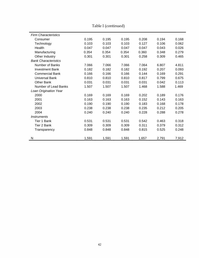
42

Table I (continued) Firm Characteristics Consumer 0.195 0.195 0.195 0.208 0.194 0.168 Technology 0.103 0.103 0.103 0.127 0.106 0.062 Health 0.047 0.047 0.047 0.047 0.043 0.026 Manufacturing 0.354 0.354 0.354 0.360 0.348 0.279 Other Industry 0.301 0.301 0.301 0.258 0.309 0.465 Bank Characteristics Number of Banks 7.066 7.066 7.066 7.064 6.807 4.811 Investment Bank 0.182 0.182 0.182 0.192 0.207 0.093 Commercial Bank 0.166 0.166 0.166 0.144 0.169 0.291 Universal Bank 0.810 0.810 0.810 0.817 0.799 0.675 Other Bank 0.031 0.031 0.031 0.031 0.042 0.113 Number of Lead Banks 1.507 1.507 1.507 1.468 1.588 1.469 Loan Origination Year 2000 0.169 0.169 0.169 0.202 0.189 0.176 2001 0.163 0.163 0.163 0.152 0.143 0.163 2002 0.190 0.190 0.190 0.183 0.168 0.178 2003 0.238 0.238 0.238 0.235 0.212 0.205 2004 0.240 0.240 0.240 0.228 0.288 0.278 Instruments Tier 1 Bank 0.531 0.531 0.531 0.542 0.463 0.318 Tier 2 Bank 0.309 0.309 0.309 0.311 0.379 0.312 Transparency 0.848 0.848 0.848 0.815 0.525 0.248 N 1,591 1,591 1,591 1,657 2,791 7,912

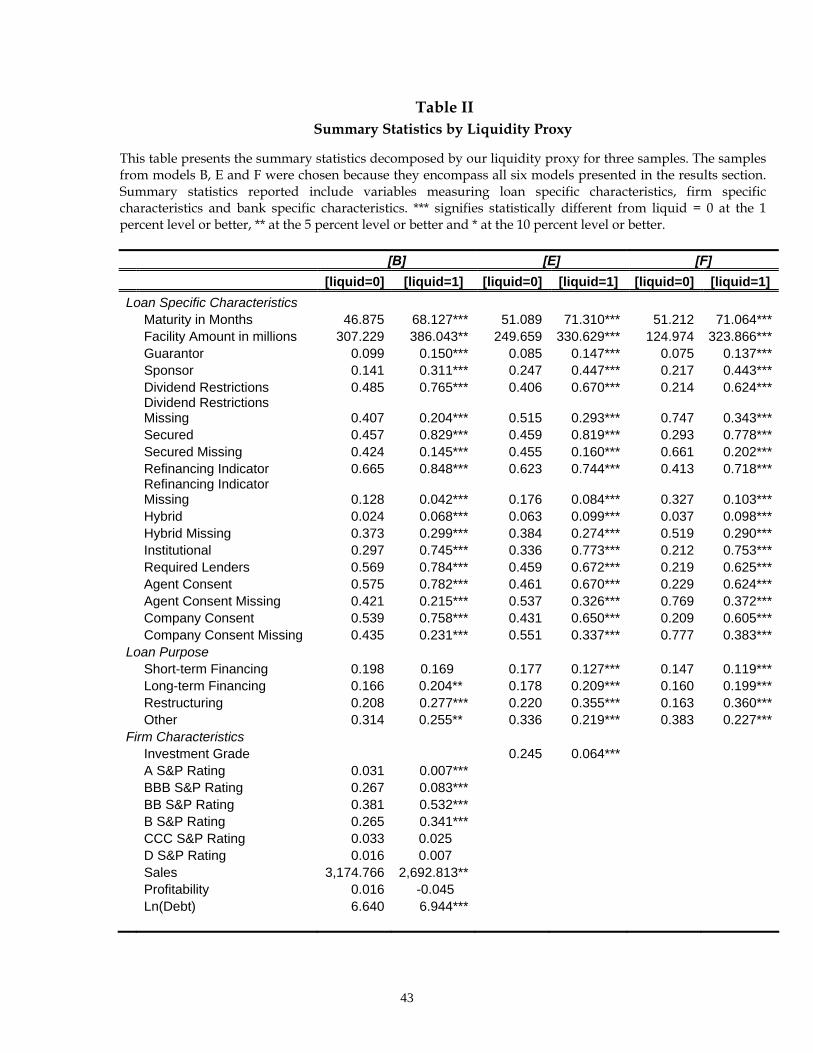
43

Table II Summary Statistics by Liquidity Proxy

This table presents the summary statistics decomposed by our liquidity proxy for three samples. The samples from models B, E and F were chosen because they encompass all six models presented in the results section. Summary statistics reported include variables measuring loan specific characteristics, firm specific characteristics and bank specific characteristics. *** signifies statistically different from liquid = 0 at the 1 percent level or better, ** at the 5 percent level or better and * at the 10 percent level or better. [B] [E] [F] [liquid=0] [liquid=1] [liquid=0] [liquid=1] [liquid=0] [liquid=1] Loan Specific Characteristics Maturity in Months 46.875 68.127*** 51.089 71.310*** 51.212 71.064*** Facility Amount in millions 307.229 386.043** 249.659 330.629*** 124.974 323.866*** Guarantor 0.099 0.150*** 0.085 0.147*** 0.075 0.137*** Sponsor 0.141 0.311*** 0.247 0.447*** 0.217 0.443*** Dividend Restrictions 0.485 0.765*** 0.406 0.670*** 0.214 0.624***

Dividend Restrictions Missing 0.407 0.204*** 0.515 0.293*** 0.747 0.343***

Secured 0.457 0.829*** 0.459 0.819*** 0.293 0.778*** Secured Missing 0.424 0.145*** 0.455 0.160*** 0.661 0.202*** Refinancing Indicator 0.665 0.848*** 0.623 0.744*** 0.413 0.718***

Refinancing Indicator Missing 0.128 0.042*** 0.176 0.084*** 0.327 0.103***

Hybrid 0.024 0.068*** 0.063 0.099*** 0.037 0.098*** Hybrid Missing 0.373 0.299*** 0.384 0.274*** 0.519 0.290*** Institutional 0.297 0.745*** 0.336 0.773*** 0.212 0.753*** Required Lenders 0.569 0.784*** 0.459 0.672*** 0.219 0.625*** Agent Consent 0.575 0.782*** 0.461 0.670*** 0.229 0.624*** Agent Consent Missing 0.421 0.215*** 0.537 0.326*** 0.769 0.372*** Company Consent 0.539 0.758*** 0.431 0.650*** 0.209 0.605*** Company Consent Missing 0.435 0.231*** 0.551 0.337*** 0.777 0.383***Loan Purpose Short-term Financing 0.198 0.169 0.177 0.127*** 0.147 0.119*** Long-term Financing 0.166 0.204** 0.178 0.209*** 0.160 0.199*** Restructuring 0.208 0.277*** 0.220 0.355*** 0.163 0.360*** Other 0.314 0.255** 0.336 0.219*** 0.383 0.227***Firm Characteristics Investment Grade 0.245 0.064*** A S&P Rating 0.031 0.007*** BBB S&P Rating 0.267 0.083*** BB S&P Rating 0.381 0.532*** B S&P Rating 0.265 0.341*** CCC S&P Rating 0.033 0.025 D S&P Rating 0.016 0.007 Sales 3,174.766 2,692.813** Profitability 0.016 -0.045 Ln(Debt) 6.640 6.944***

44

Table II (continued) Firm Characteristics Consumer 0.178 0.225** 0.175 0.226*** 0.168 0.231*** Technology 0.078 0.145*** 0.094 0.127*** 0.062 0.121*** Health 0.041 0.057 0.038 0.052* 0.026 0.046*** Manufacturing 0.360 0.343 0.352 0.336 0.279 0.327** Other Industry 0.343 0.230*** 0.341 0.259*** 0.465 0.275***Bank Characteristics Number of Banks 6.733 7.628*** 6.819 6.788 4.811 6.895*** Investment Bank 0.154 0.228*** 0.171 0.267*** 0.093 0.250*** Commercial Bank 0.209 0.093*** 0.217 0.088*** 0.291 0.100*** Universal Bank 0.767 0.882*** 0.765 0.854*** 0.675 0.856*** Other Bank 0.043 0.010*** 0.060 0.013*** 0.113 0.020*** Number of Lead Banks 1.446 1.610 1.580 1.600 1.469 1.627***Loan Origination Year 2000 0.173 0.164 0.197 0.176 0.176 0.188 2001 0.189 0.118*** 0.153 0.127* 0.163 0.120*** 2002 0.200 0.174 0.178 0.151* 0.178 0.157** 2003 0.211 0.282*** 0.187 0.253*** 0.205 0.252*** 2004 0.227 0.262 0.285 0.293 0.278 0.283 Instruments Tier 1 Bank 0.462 0.647*** 0.406 0.558*** 0.318 0.550*** Tier 2 Bank 0.311 0.306 0.378 0.382*** 0.312 0.382*** Transparency 0.850 0.845 0.496 0.573*** 0.248 0.531*** n 999 592 1,747 1,044 6,733 1,179

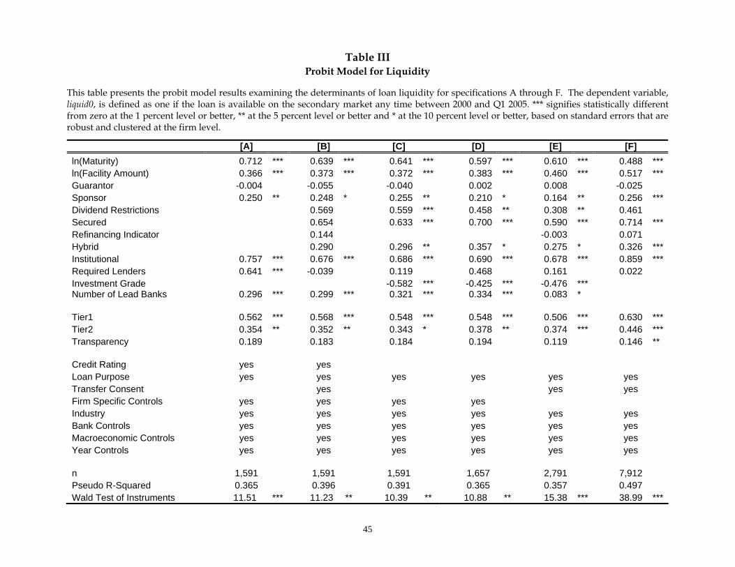
45

Table III Probit Model for Liquidity

This table presents the probit model results examining the determinants of loan liquidity for specifications A through F. The dependent variable, liquid0, is defined as one if the loan is available on the secondary market any time between 2000 and Q1 2005. *** signifies statistically different from zero at the 1 percent level or better, ** at the 5 percent level or better and * at the 10 percent level or better, based on standard errors that are robust and clustered at the firm level. [A] [B] [C] [D] [E] [F] ln(Maturity) 0.712 *** 0.639 *** 0.641 *** 0.597 *** 0.610 *** 0.488 ***ln(Facility Amount) 0.366 *** 0.373 *** 0.372 *** 0.383 *** 0.460 *** 0.517 ***Guarantor -0.004 -0.055 -0.040 0.002 0.008 -0.025 Sponsor 0.250 ** 0.248 * 0.255 ** 0.210 * 0.164 ** 0.256 ***Dividend Restrictions 0.569 0.559 *** 0.458 ** 0.308 ** 0.461 Secured 0.654 0.633 *** 0.700 *** 0.590 *** 0.714 ***Refinancing Indicator 0.144 -0.003 0.071 Hybrid 0.290 0.296 ** 0.357 * 0.275 * 0.326 ***Institutional 0.757 *** 0.676 *** 0.686 *** 0.690 *** 0.678 *** 0.859 ***Required Lenders 0.641 *** -0.039 0.119 0.468 0.161 0.022 Investment Grade -0.582 *** -0.425 *** -0.476 *** Number of Lead Banks 0.296 *** 0.299 *** 0.321 *** 0.334 *** 0.083 * Tier1 0.562 *** 0.568 *** 0.548 *** 0.548 *** 0.506 *** 0.630 ***Tier2 0.354 ** 0.352 ** 0.343 * 0.378 ** 0.374 *** 0.446 ***Transparency 0.189 0.183 0.184 0.194 0.119 0.146 ** Credit Rating yes yes Loan Purpose yes yes yes yes yes yes Transfer Consent yes yes yes Firm Specific Controls yes yes yes yes Industry yes yes yes yes yes yes Bank Controls yes yes yes yes yes yes Macroeconomic Controls yes yes yes yes yes yes Year Controls yes yes yes yes yes yes n 1,591 1,591 1,591 1,657 2,791 7,912 Pseudo R-Squared 0.365 0.396 0.391 0.365 0.357 0.497 Wald Test of Instruments 11.51 *** 11.23 ** 10.39 ** 10.88 ** 15.38 *** 38.99 ***

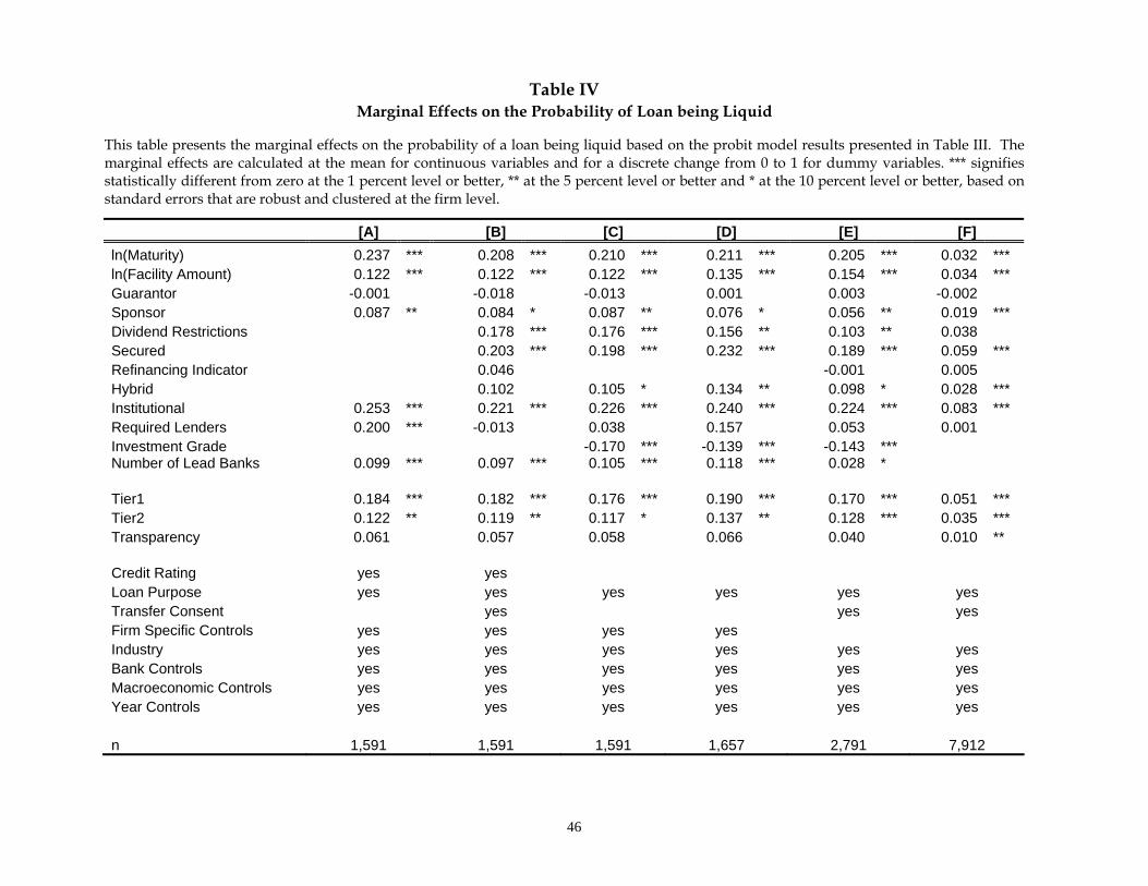
46

Table IV Marginal Effects on the Probability of Loan being Liquid

This table presents the marginal effects on the probability of a loan being liquid based on the probit model results presented in Table III. The marginal effects are calculated at the mean for continuous variables and for a discrete change from 0 to 1 for dummy variables. *** signifies statistically different from zero at the 1 percent level or better, ** at the 5 percent level or better and * at the 10 percent level or better, based on standard errors that are robust and clustered at the firm level. [A] [B] [C] [D] [E] [F] ln(Maturity) 0.237 *** 0.208 *** 0.210 *** 0.211 *** 0.205 *** 0.032 *** ln(Facility Amount) 0.122 *** 0.122 *** 0.122 *** 0.135 *** 0.154 *** 0.034 *** Guarantor -0.001 -0.018 -0.013 0.001 0.003 -0.002 Sponsor 0.087 ** 0.084 * 0.087 ** 0.076 * 0.056 ** 0.019 *** Dividend Restrictions 0.178 *** 0.176 *** 0.156 ** 0.103 ** 0.038 Secured 0.203 *** 0.198 *** 0.232 *** 0.189 *** 0.059 *** Refinancing Indicator 0.046 -0.001 0.005 Hybrid 0.102 0.105 * 0.134 ** 0.098 * 0.028 *** Institutional 0.253 *** 0.221 *** 0.226 *** 0.240 *** 0.224 *** 0.083 *** Required Lenders 0.200 *** -0.013 0.038 0.157 0.053 0.001 Investment Grade -0.170 *** -0.139 *** -0.143 *** Number of Lead Banks 0.099 *** 0.097 *** 0.105 *** 0.118 *** 0.028 * Tier1 0.184 *** 0.182 *** 0.176 *** 0.190 *** 0.170 *** 0.051 *** Tier2 0.122 ** 0.119 ** 0.117 * 0.137 ** 0.128 *** 0.035 *** Transparency 0.061 0.057 0.058 0.066 0.040 0.010 ** Credit Rating yes yes Loan Purpose yes yes yes yes yes yes Transfer Consent yes yes yes Firm Specific Controls yes yes yes yes Industry yes yes yes yes yes yes Bank Controls yes yes yes yes yes yes Macroeconomic Controls yes yes yes yes yes yes Year Controls yes yes yes yes yes yes n 1,591 1,591 1,591 1,657 2,791 7,912

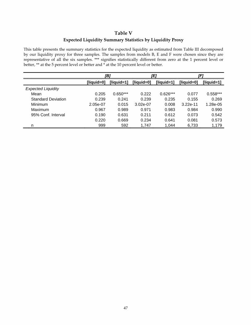
47

Table V Expected Liquidity Summary Statistics by Liquidity Proxy

This table presents the summary statistics for the expected liquidity as estimated from Table III decomposed by our liquidity proxy for three samples. The samples from models B, E and F were chosen since they are representative of all the six samples. *** signifies statistically different from zero at the 1 percent level or better, ** at the 5 percent level or better and * at the 10 percent level or better. [B] [E] [F] [liquid=0] [liquid=1] [liquid=0] [liquid=1] [liquid=0] [liquid=1] Expected Liquidity Mean 0.205 0.650*** 0.222 0.626*** 0.077 0.558*** Standard Deviation 0.239 0.241 0.239 0.235 0.155 0.269 Minimum 2.05e-07 0.015 3.02e-07 0.008 3.22e-11 1.28e-05 Maximum 0.967 0.989 0.971 0.983 0.984 0.990 95% Conf. Interval 0.190 0.631 0.211 0.612 0.073 0.542 0.220 0.669 0.234 0.641 0.081 0.573 n 999 592 1,747 1,044 6,733 1,179

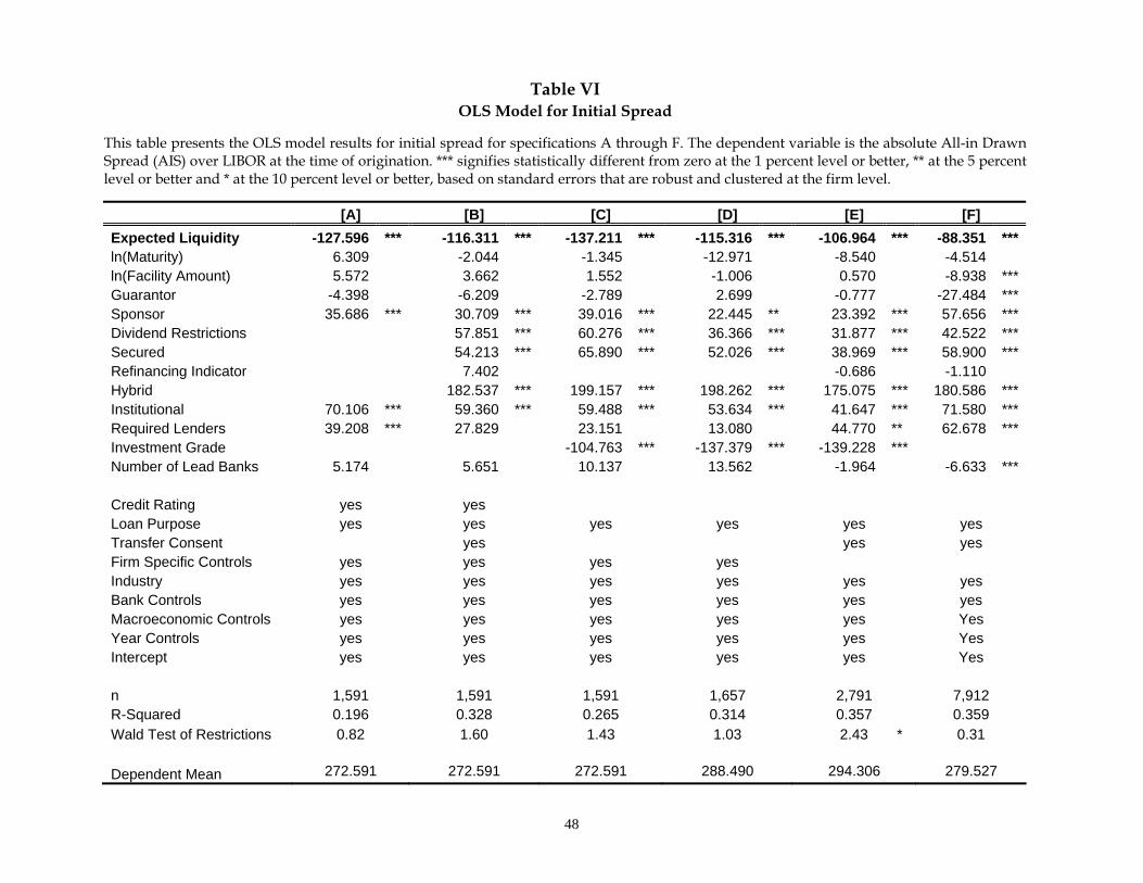
48

Table VI OLS Model for Initial Spread

This table presents the OLS model results for initial spread for specifications A through F. The dependent variable is the absolute All-in Drawn Spread (AIS) over LIBOR at the time of origination. *** signifies statistically different from zero at the 1 percent level or better, ** at the 5 percent level or better and * at the 10 percent level or better, based on standard errors that are robust and clustered at the firm level.

[A] [B] [C] [D] [E] [F] Expected Liquidity -127.596 *** -116.311 *** -137.211 *** -115.316 *** -106.964 *** -88.351 ***ln(Maturity) 6.309 -2.044 -1.345 -12.971 -8.540 -4.514 ln(Facility Amount) 5.572 3.662 1.552 -1.006 0.570 -8.938 ***Guarantor -4.398 -6.209 -2.789 2.699 -0.777 -27.484 ***Sponsor 35.686 *** 30.709 *** 39.016 *** 22.445 ** 23.392 *** 57.656 ***Dividend Restrictions 57.851 *** 60.276 *** 36.366 *** 31.877 *** 42.522 ***Secured 54.213 *** 65.890 *** 52.026 *** 38.969 *** 58.900 ***Refinancing Indicator 7.402 -0.686 -1.110 Hybrid 182.537 *** 199.157 *** 198.262 *** 175.075 *** 180.586 ***Institutional 70.106 *** 59.360 *** 59.488 *** 53.634 *** 41.647 *** 71.580 ***Required Lenders 39.208 *** 27.829 23.151 13.080 44.770 ** 62.678 ***Investment Grade -104.763 *** -137.379 *** -139.228 *** Number of Lead Banks 5.174 5.651 10.137 13.562 -1.964 -6.633 *** Credit Rating yes yes Loan Purpose yes yes yes yes yes yes Transfer Consent yes yes yes Firm Specific Controls yes yes yes yes Industry yes yes yes yes yes yes Bank Controls yes yes yes yes yes yes Macroeconomic Controls yes yes yes yes yes Yes Year Controls yes yes yes yes yes Yes Intercept yes yes yes yes yes Yes n 1,591 1,591 1,591 1,657 2,791 7,912 R-Squared 0.196 0.328 0.265 0.314 0.357 0.359 Wald Test of Restrictions 0.82 1.60 1.43 1.03 2.43 * 0.31 Dependent Mean 272.591 272.591 272.591 288.490 294.306 279.527

49

Table VII OLS Model for Initial Relative Spread

This table presents the OLS model results for initial relative spread for specifications A through F. The dependent variable is the initial relative spread measured as the ratio of the initial All-in Drawn Spread over LIBOR and the LIBOR at the time of origination. *** signifies statistically different from zero at the 1 percent level or better, ** at the 5 percent level or better and * at the 10 percent level or better, based on standard errors that are robust and clustered at the firm level.

[A] [B] [C] [D] [E] [F] Expected Liquidity -0.700 *** -0.601 *** -0.727 *** -0.640 *** -0.625 *** -0.464 ***ln(Maturity) 0.005 -0.033 -0.031 -0.114 ** -0.095 ** -0.058 ***ln(Facility Amount) 0.027 0.007 -0.006 0.004 0.027 -0.039 ***Guarantor 0.002 0.005 0.031 0.072 0.018 -0.178 ***Sponsor 0.264 *** 0.220 *** 0.274 *** 0.204 *** 0.214 *** 0.373 ***Dividend Restrictions 0.201 ** 0.219 ** 0.100 0.070 0.124 ** Secured 0.266 *** 0.309 *** 0.280 *** 0.298 *** 0.336 ***Refinancing Indicator -0.019 -0.052 -0.029 Hybrid 1.395 *** 1.524 *** 1.543 *** 1.302 *** 1.354 ***Institutional 0.375 *** 0.324 *** 0.321 *** 0.268 *** 0.180 *** 0.380 ***Required Lenders 0.224 *** 0.180 0.196 0.174 0.304 *** Investment Grade -0.542 *** -0.699 *** -0.726 *** Number of Lead Banks -0.044 -0.028 -0.006 -0.039 -0.026 -0.070 *** Credit Rating yes yes Loan Purpose yes yes yes yes yes yes Firm Specific Controls yes yes yes yes Industry yes yes yes yes yes yes Bank Controls yes yes yes yes yes yes Macroeconomic Controls yes yes yes yes yes yes Year Controls yes yes yes yes yes yes Intercept yes yes yes yes yes yes n 1,591 1,591 1,591 1,657 2,791 7,912 R-Squared 0.525 0.603 0.557 0.592 0.604 0.580 Wald Test of Restrictions 0.960 1.860 1.75 1.43 2.51 * 0.74 Dependent Mean 1.520 1.520 1.520 1.576 1.624 1.523

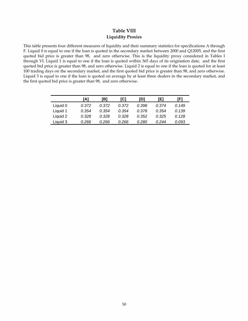
50

Table VIII Liquidity Proxies

This table presents four different measures of liquidity and their summary statistics for specifications A through F. Liquid 0 is equal to one if the loan is quoted in the secondary market between 2000 and Q12005, and the first quoted bid price is greater than 98, and zero otherwise. This is the liquidity proxy considered in Tables I through VI. Liquid 1 is equal to one if the loan is quoted within 365 days of its origination date, and the first quoted bid price is greater than 98, and zero otherwise. Liquid 2 is equal to one if the loan is quoted for at least 100 trading days on the secondary market, and the first quoted bid price is greater than 98, and zero otherwise. Liquid 3 is equal to one if the loan is quoted on average by at least three dealers in the secondary market, and the first quoted bid price is greater than 98, and zero otherwise.

[A] [B] [C] [D] [E] [F] Liquid 0 0.372 0.372 0.372 0.398 0.374 0.149 Liquid 1 0.354 0.354 0.354 0.378 0.354 0.139 Liquid 2 0.328 0.328 0.328 0.352 0.325 0.128 Liquid 3 0.266 0.266 0.266 0.280 0.244 0.093

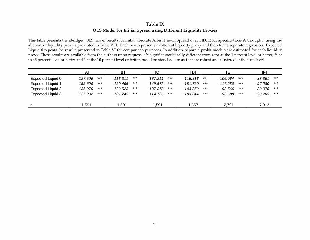
51

Table IX OLS Model for Initial Spread using Different Liquidity Proxies

This table presents the abridged OLS model results for initial absolute All-in Drawn Spread over LIBOR for specifications A through F using the alternative liquidity proxies presented in Table VIII. Each row represents a different liquidity proxy and therefore a separate regression. Expected Liquid 0 repeats the results presented in Table VI for comparison purposes. In addition, separate probit models are estimated for each liquidity proxy. These results are available from the authors upon request. *** signifies statistically different from zero at the 1 percent level or better, ** at the 5 percent level or better and * at the 10 percent level or better, based on standard errors that are robust and clustered at the firm level. [A] [B] [C] [D] [E] [F] Expected Liquid 0 -127.596 *** -116.311 *** -137.211 *** -115.316 ** -106.964 *** -88.351 *** Expected Liquid 1 -153.896 *** -130.466 *** -149.673 *** -151.730 *** -117.250 *** -97.080 *** Expected Liquid 2 -136.976 *** -122.523 *** -137.878 *** -103.359 *** -92.566 *** -80.076 *** Expected Liquid 3 -127.202 *** -101.745 *** -114.736 *** -103.044 *** -93.688 *** -93.205 *** n 1,591 1,591 1,591 1,657 2,791 7,912

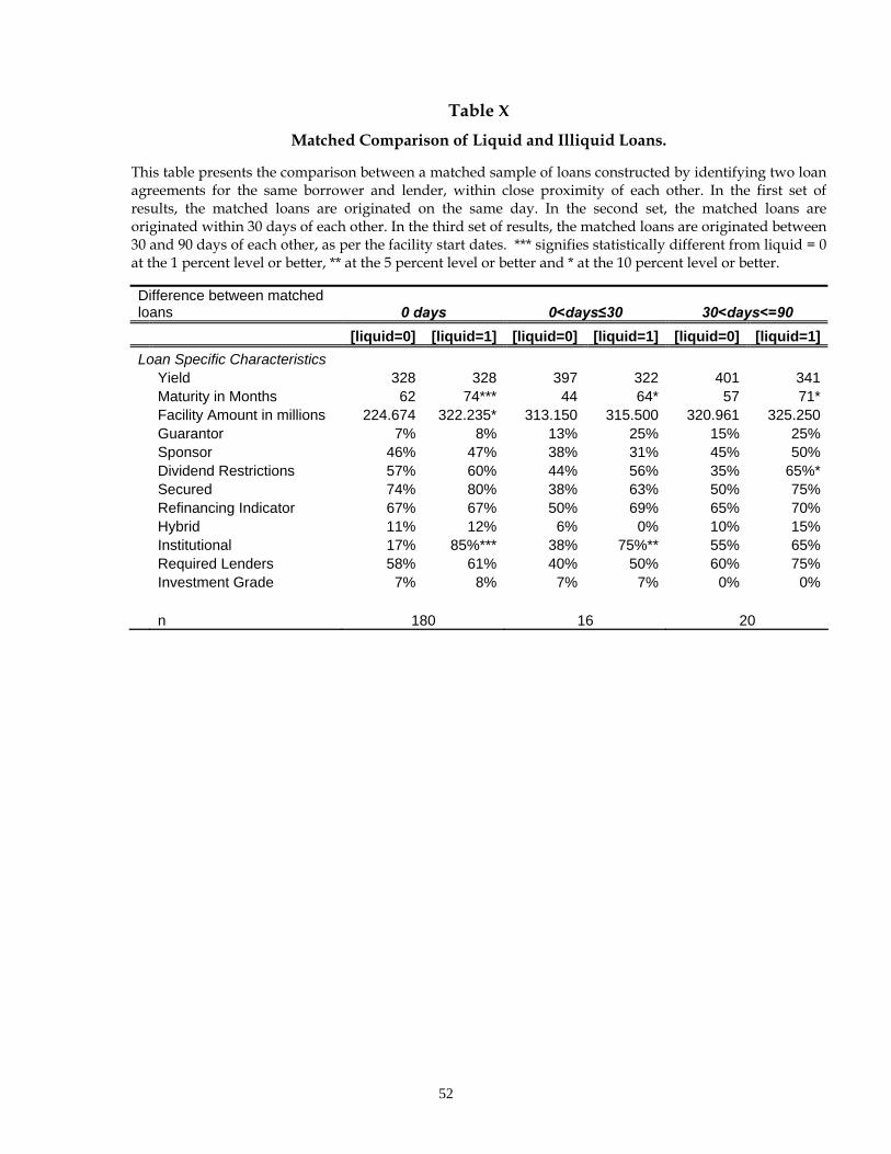
52

Table X

Matched Comparison of Liquid and Illiquid Loans.

This table presents the comparison between a matched sample of loans constructed by identifying two loan agreements for the same borrower and lender, within close proximity of each other. In the first set of results, the matched loans are originated on the same day. In the second set, the matched loans are originated within 30 days of each other. In the third set of results, the matched loans are originated between 30 and 90 days of each other, as per the facility start dates. *** signifies statistically different from liquid = 0 at the 1 percent level or better, ** at the 5 percent level or better and * at the 10 percent level or better.

Difference between matched loans 0 days 0<days≤30 30<days<=90 [liquid=0] [liquid=1] [liquid=0] [liquid=1] [liquid=0] [liquid=1]Loan Specific Characteristics Yield 328 328 397 322 401 341 Maturity in Months 62 74*** 44 64* 57 71* Facility Amount in millions 224.674 322.235* 313.150 315.500 320.961 325.250 Guarantor 7% 8% 13% 25% 15% 25% Sponsor 46% 47% 38% 31% 45% 50% Dividend Restrictions 57% 60% 44% 56% 35% 65%* Secured 74% 80% 38% 63% 50% 75% Refinancing Indicator 67% 67% 50% 69% 65% 70% Hybrid 11% 12% 6% 0% 10% 15% Institutional 17% 85%*** 38% 75%** 55% 65% Required Lenders 58% 61% 40% 50% 60% 75% Investment Grade 7% 8% 7% 7% 0% 0% n 180 16 20

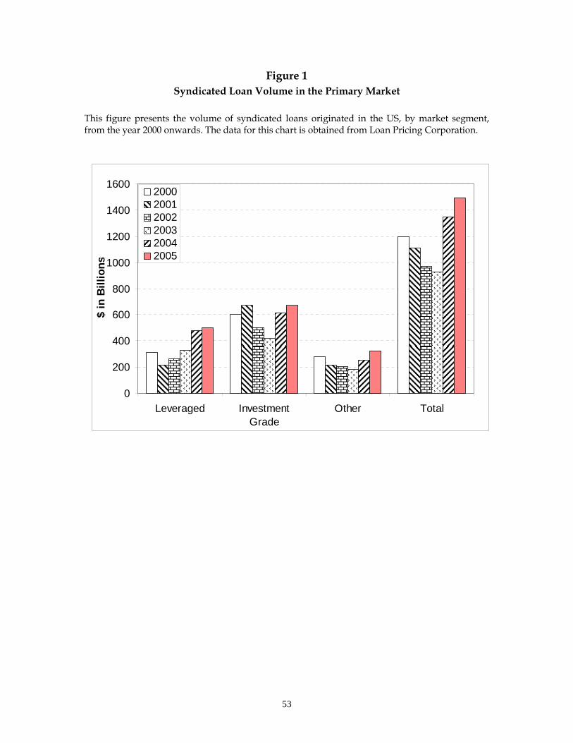
53

0

200

400

600

800

1000

1200

1400

1600

Leveraged InvestmentGrade

Other Total

$ in

Bill

ions

200020012002200320042005

Figure 1 Syndicated Loan Volume in the Primary Market

This figure presents the volume of syndicated loans originated in the US, by market segment, from the year 2000 onwards. The data for this chart is obtained from Loan Pricing Corporation.

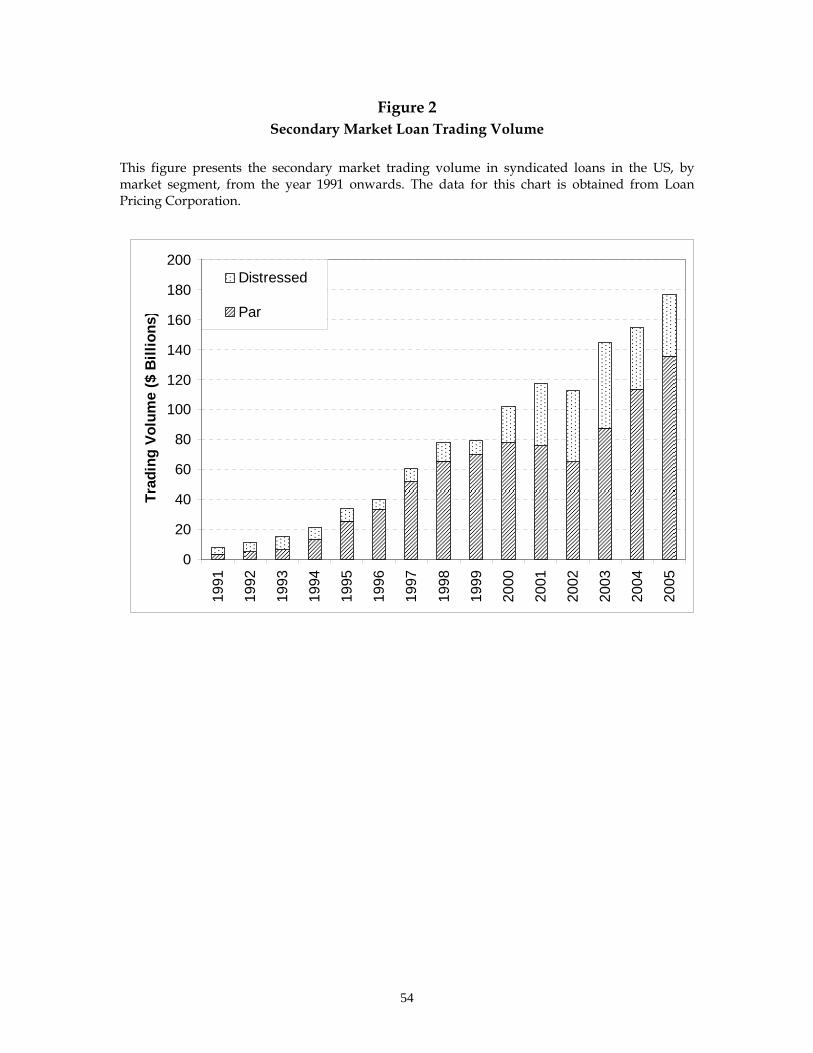
54

0

20

40

60

80

100

120

140

160

180

200

1991

1992

1993

1994

1995

1996

1997

1998

1999

2000

2001

2002

2003

2004

2005

Trad

ing

Volu

me

($ B

illio

ns)

Distressed

Par

Figure 2 Secondary Market Loan Trading Volume

This figure presents the secondary market trading volume in syndicated loans in the US, by market segment, from the year 1991 onwards. The data for this chart is obtained from Loan Pricing Corporation.

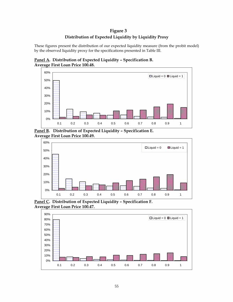
55

Figure 3 Distribution of Expected Liquidity by Liquidity Proxy

These figures present the distribution of our expected liquidity measure (from the probit model) by the observed liquidity proxy for the specifications presented in Table III. Panel A. Distribution of Expected Liquidity – Specification B. Average First Loan Price 100.48.

0%

10%

20%

30%

40%

50%

60%

0.1 0.2 0.3 0.4 0.5 0.6 0.7 0.8 0.9 1

Liquid = 0 Liquid = 1

Panel B. Distribution of Expected Liquidity – Specification E. Average First Loan Price 100.49.

0%

10%

20%

30%

40%

50%

60%

0.1 0.2 0.3 0.4 0.5 0.6 0.7 0.8 0.9 1

Liquid = 0 Liquid = 1

Panel C. Distribution of Expected Liquidity – Specification F. Average First Loan Price 100.47.

0%

10%

20%

30%

40%

50%

60%

70%

80%

90%

0.1 0.2 0.3 0.4 0.5 0.6 0.7 0.8 0.9 1

Liquid = 0 Liquid = 1