Embed Size (px)
Citation preview
*This paper was recommended for publication in revised formby Associate Editor P. Dorato. Corresponding author Y. Fang.Tel. 00852 2788 9965; Fax 00852 2788 7791 E-mail [email protected] of Electronic Engineering, City University of
Hong Kong, Tat Chee Avenue, Kowloon, Hong Kong
PII: S0005–1098(98)00091–0Automatica, Vol. 34, No. 11, pp. 1459—1462, 1998( 1998 Elsevier Science Ltd. All rights reserved
Printed in Great Britain0005-1098/98 $—see front matter
Technical Communique
Iterative Learning Control of Linear Discrete-TimeMultivariable Systems*
YONG FANG- and TOMMY W. S. CHOW-
Key Words—Discrete-time systems; uncertain systems; iterative learning control; 2-D system theory; closedloop.
Abstract—The authors present an iterative learning control rulefor linear discrete-time multivariable systems. The control ruleassures a zero output error for the whole desired trajectory afteronly one learning iteration. The robustness of the control ruleis studied and two numerical examples are used to validatethe new control rule. ( 1998 Elsevier Science Ltd. All rightsreserved.
1. IntroductionA control system which has a desired response for a finite timeinterval is widely applied for processing industries, painting,sealing, and robotics pick-and-place operations. Generally, a dy-namic controller in a closed-loop system that cannot achieveconsistently perfect tracking (Gupta and Sinha, 1996) becausethe required responses differ for each task. In order to obtaina control sequence defined on a finite time interval that givea perfect trajectory tracking performance, one must consider thesystem as an iterative control system such that the outputaccuracy can be iteratively improved. Iterative learning controlwas firstly introduced by Arimoto et al (1984). Since then, manysimple learning control approaches have been studied (Moore,1993; Amann et al., 1996). However, in all these proposed learn-ing algorithms many iterations are needed to achieve the re-quired accuracy.
Recently, two-dimensional (2D) system theory was introducedto establish a suitable mathematical model to clearly describeboth the dynamics of the control system and the behavior of thelearning process, and thus design the learning control algo-rithms for discrete-time systems (Geng et al., 1990). Also, Chowand Fang (1998) proposed an iterative learning control methodfor continuous-time systems based on 2D continuous-discretesystem model. Kurek and Zaremba (1993) proposed an effectivealgorithm in which control error converges to zero in finiteiterations. They also proposed a theoretical algorithm which iscapable of driving the control error to zero after only onelearning iteration. In other words, the new control input can bedetermined in accordance with the initialized input withoutfurther iterations. This building process, however, requiresnew state information of the system which is yielded by the newcontrol input. This approach is not practical because the newcontrol input is, in fact, an unknown. To overcome this diffi-culty, an estimated system state was employed in their proposedalgorithm at an expense of output performance. As a result, thisleads to an increase of control (Kurek and Zaremba, 1993). Inaddition, the effectiveness and the convergence of the controlalgorithm cannot be always guaranteed. This shortcoming isillustrated in ‘‘Example 2’’ of this paper.
In this paper, we propose a learning algorithm that assuresthe desired trajectory to be accurately tracked after only one
learning iteration. In the proposed algorithm, the difficulty ofKurek’s algorithm is overcome. We also derive the necessaryand sufficient conditions for the convergence of the proposedalgorithm applying to the control systems with unknown plantparameters. Two examples are used to demonstrate that ourproposed control algorithm is more effective than Kurek’s algo-rithm in terms of output convergence.
2. Problem formulationThis work is concerned with a linear discrete-time multi-
variable system represented by
x (t#1)"Ax (t)#Bu (t), (1)
y(t)"Cx(t), (2)
where x3Rn is the state vector; u3Rm is the input vector; y3Rp
is the output vector; and A, B, C are real matrices of appropriatedimensions. Without loss of generality, it is assumed that thematrices B and C are full rank. If the initial condition x(0)"x
0,
this system has the following well-known solution:
y(t)"CAtx0#
t~1+i/0
CAt~1~iBu(i). (3)
For a given trajectory Myd(t), t"1,2,2 , NN, our goal is to
design a control sequence Mu(t),t"0, 1,2 , N!1N for the sys-tem (1), (2) with the initial condition x(0)"x
0such that the
given trajectory can be perfectly tracked. Obviously, a controlsequence can be obtained when the system is known exactly.However, the system matrices A, B and C are not usually knownand only their estimate values are available. It is usually neces-sary that each new control sequence is created in each iterationfrom the pre-existing control sequence. The generation of theiteration can be expressed by
u (t)=u (t)#*u(t). (4)
Despite the fact that many studies were performed on the iter-ative learning control rule, *u(t), for both discrete systems andcontinuous systems (Moore, 1993; Chow and Fang, 1998), a newderivation of the *u (t), which assures the output error can bedriven to zero within one control iteration, is presented in thenext section.
3. Design of learning control ruleThe design of an appropriate iterative learning control rule is
crucial to the tracking performance of a control system. Usually,the current state and errors information of the system are neces-sary for the learning rule. The learning rule proposed hererequires the state information of the closed-loop system witha state feedback. We firstly present the following two lemmas.
¸emma 1. There exists matrices K1
and K2
such thatI!CBK
1"0 and !CA#CBK
2"0, where I is an identity
matrix of appropriate dimensions, iff matrix CB is full-row rank,and K
1and K
2can always be calculated by
K1"(CB)T[CB(CB)T]~1 and K
2"K
1CA, (5)
where T denotes the transpose.
1459
By applying the Kroneck—Capelli theorem (Kaczorek, 1985),the lemma is easy to prove.
¸emma 2. If the condition of Lemma 1 is satisfied, for any inputsequence, u(t), t"0,1,2 ,N!1, and K
1and K
2which are
calculated according to equation (5), let
u*(t)"(I!K1CB)u (t)#K
1y$(t#1), (6)
then the closed-loop system
xL (t#1)"(A!BK2)xL (t)#Bu*(t), (7)
yL (t)"CxL (t) (8)
has the desired output, y$(t), t"1, 2,2 , N.
Proof. According to equation (3), the output of the closed-loopsystem (7), (8) can be expressed as follows:
yL (t)"C(A!BK2)tx
0#
t~1+i/0
C(A!BK2)t~1~i
]B[(I!K1CB)u(i)#K
1y$(i#1)]. (9)
By Lemma 1, for t'0, we have C(A!BK2)t"0. Thus,
yL (t)"CB(I!K1CB)u(t!1)#CBK
1y$(t)
"(I!CBK1)CBu(t!1)#CBK
1y$(t)
"y$(t).
u*(t), which is the input of the closed-loop system (7), (8), isconstructed by the input u(t) of system (1), (2). Based onLemma 2, the output of the closed-loop system (7), (8) are alwaysidentical to the desired trajectory for any input signal u(t) in u*(t).We have designed an output reference system according tosystem (1), (2). The system output does not depend on the inputsignal u(t) in u*(t), which implies that the signal u(t) in u*(t) has noeffect for the output of the closed-loop system (7), (8). In thefollowing applications, the input signal u(t) in u*(t) is identical asthe input of system (1), (2).
Our objective is to find the control sequence such that thesystem (1), (2) has the desired output. For system (1), (2) with anyinitial input sequence, u(t), t"0,1,2 , N!1, and a given de-sired output, the closed-loop system (7), (8) with the input u*(t)has the desired output if the condition of Lemma 1 is satisfied.The state information of the closed-loop system (7), (8) areutilized to formulate the new control input of system (1), (2). Thefollowing theorem describes clearly the solution of the problem.
¹heorem 1. The following iterative learning control rule drivesthe control error to zero for the whole desired trajectory afteronly one learning iteration if the condition of Lemma 1 issatisfied:
u(t)=u* (t)!K2xL (t), (10)
where matrix K*2
is calculated by equation (5), u*(t) is defined byequation (6) and xL (t) is the state vector of system (7).
Proof. Applying the control input (10) to system (1), (2), weobtain
x(t#1)"Ax(t)#B[u*(t)!K2xL (t)] and y(t)"Cx(t). (11)
From Lemma 2, we know that the output of the system (7), (8) isidentical to the desired trajectory. Namely, y
$(t)"yL (t). Defining
the tracking error e (t)"y$(t )!y(t), for 14t4N. Therefore,
the error equations are derived by equations (1) and (8)
e(t!1)"y$(t#1)!y(t#1)
"CxL (t#1)#Cx(t#1)
"C (A!BK2)xL (t )#Bu*(t)!CAx(t)
!CB[u*(t)!K2xL (t)],
where 04t4N!1. Since !CA#CBK2"0, it follows that
e(t#1)"!CAx(t)#CBK2xL (t )"!CA[x(t)!xL (t)]. (12)
On the other hand, by equations (7) and (11) we have
x (t#1)!xL (t#1)"A[x (t)!xL (t)] (13)
holds. Since both system (1), (2) and system (7), (8) have the sameinitial condition x (0)"xL (0)"x
0, x (t)!xL (t)"0 holds for
0(t4N. Hence, from equation (12) we get for e (t#1)"0 for04t4N!1. That is, e (t)"0 holds for 0(t4N. This com-pletes the proof. K
According to equations (6) and (10), the iterative learningcontrol rule (10) can be given by
u (t)f(I!K1CB)u(t)#K
1y$(t#1)!K
2xL (t). (14)
By using the iterative learning control rule, the new controlinput can be determined by the current control input, the desiredtrajectory, and the state information of the closed-loop system(7). Obviously, this is a more effective learning rule than otherlearning methods which usually require many iterations.
For the learning rule (14), the learning matrices are requiredto be calculated by equation (5). This implies that the learningrule depends upon the system matrices A, B and C which are notusually known. Only estimated values of A, B and C are avail-able. As a result, many learning iterations are inevitably re-quired. It is also noticed that the error has not been included inthe learning rule (14). When the system matrices are not known,the error term is essential for the derivation of the iterative rule.In view of the above reasons, equation (14) is rewritten as thefollowing equivalent form:
u(t )fu(t)!K1CBu(t)#K
1y$(t!1)!K
1y(t#1)
#K1y(t#1)!K
2xL (t)
"u (t)!K1CBu(t)#K
1e(t#1)#K
1C[Ax(t)#Bu(t)]
!K2xL (t)
"u (t)#K1e (t#1)#K
1CAx(t)!K
2xL (t)
"u (t)#K1e (t#1)#K
2[x(t)!xL (t)]. (15)
Namely,
*u(t)"Kie(t#1)#K
2[x (t)!xL (t)] (16)
Obviously, only the learning matrices K1
and K2
are required.The control rule (15) has certain similarity to that of Kurek andZaremba’s (1993), *u(t)"K
1e(t#1)#K
2[x(t)!x@ (t)], which
drives the control error to zero after only one iteration. Theircontrol rule requires the information of the current system statex@(t) yielded by the new control sequence, which is not available.In the implementation of the control rule, this shortcoming isresolved by estimating the current system state, x@ (t), by usingthe input sequence u*(t). Consequently, the control error cannot be driven to zero after one iteration. The convergence ishardly guaranteed, as demonstrated in Example 2.
To determine the conditions that the estimated learningmatrices K
1and K
2should satisfy, let subscript k denote the kth
iteration, and KI1
and KI2
denote the estimates of K1
and K2.
According to Lemmas 1, 2 and equation (11), x (t)!xL (t)"0,the control error of the k#1th iteration is given by
ek`1
(t#1)"y$(t#1)!y
k`1(t#1)
"C (A!BK2)xL
k`1(t)
#CB[u(t)#K1ek(t#1)#K
2xk(t)]
!CAxk`1
(t)!CB[u(t)#KI1ek(t#1)
#KI2xk(t)!KI
2xLk`1
(t)]
"(1!CBKI1)e
k(t#1)#(CA!CBKI
2)
][xk(t)!x
k`1(t)]. (17)
Let gk(t#1)"x
k~1(t)!x
k(t), then from equation (11) with KI
1and KI
2, we can obtain
gk(t#1)"(A!BKI
2)g
k(t)!BKI
1e (t) (18)
1460 Technical Communiques
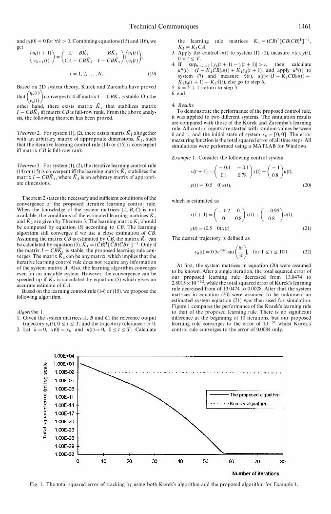
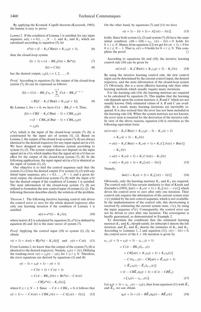
Fig. 1. The total squared error of tracking by using both Kurek’s algorithm and the proposed algorithm for Example 1.
and gk(0)"0 for ∀k'0. Combining equations (15) and (16), we
get
Agk(t#1)
ek`1
(t) B"AA!BKI
2CA!CBKI
2
!BKI1
I!CBKI1B A
gk(t)
ek(t)B ,
t"1, 2,2 , N. (19)
Based on 2D system theory, Kurek and Zaremba have proved
that Agk(t)
ek(t)B converges to 0 iff matrix I!CBKI
1is stable. On the
other hand, there exists matrix KI1
that stabilizes matrixI!CBKI
1iff matrix CB is full-row rank. From the above analy-
sis, the following theorem has been proved.
¹heorem 2. For system (1), (2), there exists matrix KI1
altogetherwith an arbitrary matrix of appropriate dimensions, KI
2, such
that the iterative learning control rule (14) or (15) is convergentiff matrix CB is full-row rank.
¹heorem 3. For system (1), (2), the iterative learning control rule(14) or (15) is convergent iff the learning matrix KI
1stabilizes the
matrix I!CBKI1, where KI
2is an arbitrary matrix of appropri-
ate dimensions.
Theorem 2 states the necessary and sufficient conditions of theconvergence of the proposed iterative learning control rule.When the knowledge of the system matrices (A, B, C) is notavailable, the conditions of the estimated learning matrices KI
1and KI
2are given by Theorem 3. The learning matrix K
1should
be computed by equation (5) according to CB. The learningalgorithm still converges if we use a close estimation of CB.Assuming the matrix CB is estimated by CI B, the matrix KI
1can
be calculated by equation (5), KI1"(CI B)T[CI B(CM B)T]~1. Only if
the matrix I!CBKI1
is stable, the proposed learning rule con-verges. The matrix KI
2can be any matrix, which implies that the
iterative learning control rule does not require any informationof the system matrix A. Also, the learning algorithm convergeseven for an unstable system. However, the convergence can bespeeded up if KI
2is calculated by equation (5) which gives an
accurate estimate of CA.Based on the learning control rule (14) or (15), we propose the
following algorithm.
Algorithm 1.1. Given the system matrices A, B and C; the reference output
trajectory yr(t), 04t4¹; and the trajectory tolerance e'0.
2. Let k"0, x (0)"x0
and u(t)"0, 04t4¹. Calculate
the learning rule matrices K1"(CB)T[CB(CB)T]~1,
K2"K
1CA.
3. Apply the control u(t) to system (1), (2), measure x (t), y(t),0(t4¹.
4. If sup04t(¹D y
$(t#1)!y(t#1) D'e, then calculate
u*(t)"(I!K1CB)u(t)#K
1y$(t#1), and apply u*(t) to
system (7) and measure xL (t), u(t)f(I!K1CB)u (t)#
K1y$(t#1)!K
2xL (t), else go to step 6.
5. k"k#1, return to step 3.6. end.
4. ResultsTo demonstrate the performance of the proposed control rule,
it was applied to two different systems. The simulation resultsare compared with those of the Kurek and Zaremba’s learningrule. All control inputs are started with random values between0 and 1, and the initial state of system x
0"[0, 0]. The error
measuring function is the total squared error of all time steps. Allsimulations were performed using a MATLAB for Windows.
Example 1. Consider the following control system:
x (t#1)"A!0.1
0.1
!0.1
0.78 Bx(t)#A!1
0.8 Bu(t),
y (t)"(0.5 0)x (t), (20)
which is estimated as
x(t#1)"A!0.2
0
0
0.8Bx (t)#A!0.95
0.8 B u(t),
y(t)"(0.5 0)x(t). (21)
The desired trajectory is defined as
y$(t)"0.5et@50 sin A
6t
50B, for 14t4100. (22)
At first, the system matrices in equation (20) were assumedto be known. After a single iteration, the total squared error ofour proposed learning rule decreased from 13.0474 to2.8015]10~32, while the total squared error of Kurek’s learningrule decreased from of 13.0474 to 0.0028. After that the systemmatrices in equation (20) were assumed to be unknown, anestimated system equation (21) was then used for simulation.Figure 1 compares the performance of the Kurek’s learning ruleto that of the proposed learning rule. There is no significantdifference at the beginning of 10 iterations, but our proposedlearning rule converges to the error of 10~31 whilst Kurek’scontrol rule converges to the error of 0.0084 only.
Technical Communiques 1461
Fig. 2. The total squared error of tracking by using both Kurek’s algorithm and the proposed algorithm for Example 2.
Example 2. Consider the changed control system:
x(t#1)"A!1.1
0.1
!0.1
0.78 B x(t)#A!1
0.8 B u(t),
y(t)"(0.5 0)x(t). (23)
which is estimated as
x (t#1)"A!1
0
0
0.8B x (t)#A!0.95
0.8 B u (t),
y(t)"(0.5 0)x (t). (24)
If the system matrices in equation (23) were known, the totalsquared error of our proposed learning rule decreased from2.4909]107 to 3.7246]10~26 while the total squared errorof Kurek’s learning rule increased to 7.3087]108 from2.4909]107. It is also noticed that the error level of Kurek’slearning rule could not be reduced for further iterations. Whenthe system matrices in equation (23) was unknown, the estimatedsystem (24) was used. Figure 2 shows the convergence of theerror. The total squared error of our proposed learning ruleconverged to the error of about 10~25, whilst the error did notconverge to a level comparably small when Kurek’s learningrule was applied.
5. ConclusionsAn iterative learning control rule is presented for linear dis-
crete-time multivariable systems. The system governed by theproposed control rule tracks the desired trajectory accuratelyafter only one learning iteration. Necessary and sufficient condi-tions for the convergence are derived. The robustness of theproposed control rule is also discussed. The convergence isassured even if there is small perturbations of the system para-meters. As a result, the proposed learning control rule is capable
of maintaining an excellent performance when system para-meters are unknown, or change during operation. Another ma-jor advantage of the proposed control rule is that no informa-tion yielded by the new control input is required. This enablesthe control system to drive the output error to a negligible value.Simulation results show that the proposed control rule is ca-pable of driving the control error to a very small level, which isa significant improvement compared to the control rule pro-posed by Kurek and Zaremba.
ReferencesAmann, N., D. H. Owens and E. Rogers (1996). Iterative learning
control for discrete-time systems with exponential rate ofconvergence. IEE Proc. Control ¹heory Appl., 143, 217—224.
Arimoto, S., S. Kawamura and F. Miyazaki (1984). Betteringoperation of robots by learning. Proc. 23rd IEEE Conf. onDecision and Control, pp. 1064—1069.
Chow, T. W. S. and Y. Fang (1998). An iterative learning controlmethod for continuous-time systems based on 2-D systemtheory. IEEE ¹rans. Circuits Systems—I, 45, 683—689.
Geng, Z., R. Carroll and J. Xies (1990). Two-dimensional modeland algorithm analysis for a class of iterative learning controlsystems. Int. J. Control., 52, 833—862.
Gupta, M. M. and N. K. Sinha (1987). Intelligent ControlSystem. IEEE Neural Networks Council, Sponsor, IEEEPress, New York.
Kaczorek, T. (1985). ¹wo-Dimensional ¸inear Systems. SpringerBerlin.
Kurek, J. E. and M. B. Zaremba (1993). Iterative learningcontrol synthesis based on 2-D system theory. IEEE ¹rans.Automat. Control, 38, 121—125.
Moore, K. L. (1993). Iterative ¸earning Control for DeterministicSystem, Advances in Industrial Control Series. SpringerLondon.
1462 Technical Communiques