INVESTIGATING FAST FOLDING OF RNA PSEUDOKNOT VPK WITH ANULTRAFAST MICROFLUIDIC MIXER

By

Andreas John Meindl

A THESIS

Submitted toMichigan State University

in partial fulfillment of the requirementsfor the degree of

MASTER OF SCIENCE

Physics

2012

ABSTRACT

INVESTIGATING FAST FOLDING OF RNA PSEUDOKNOT VPK WITHAN ULTRAFAST MICROFLUIDIC MIXER

By

Andreas John Meindl

Despite advances in understanding the theory behind RNA folding, ab initio prediction of

the folding process has not been achieved yet. Given only the sequence information we still

cannot tell the precise three-dimensional structure of neither RNA nor protein. Knowing the

kinetics of folding we hope to learn more about the arrangement of secondary and tertiary

structure.

For that reason we investigated the folding process of RNA pseudoknot VPK with our

microfluidic mixing device. VPK (variant pseudoknot) is a variant of the mouse mammary

tumor virus (MMTV) pseudoknot and it was specifically designed to prevent the formation

of alternative base pairings in the stem regions. Using two differently labeled samples,

VPK-2AP and F-VPK, and high and low salt folding conditions, we analyzed the folding

process and determined the different folding rates. Our results match very well with recently

published findings, but they also raise the possible existence of folding transitions not seen

in T-jump experiments. The measured folding times are in the range of 0.5 to several

milliseconds. The folding process seems to have different pathways with one of the stems of

the pseudoknot forming before, perhaps even initiating the folding of the other.

ACKNOWLEDGMENT

Writing a thesis can only prove successful with an interested and motivating mentor and

advisor. Therefore, I am very grateful to Lisa Lapidus for the time and effort she invested

in instructing me and discussing with me.

I would like to thank my fellow group members for their expertise and the good working

atmosphere. Ling Wu introduced me to our setup knowledgeably and laid the base for the

success of my work. Terry Ball’s help with buffers and the RNA samples was crucial for the

good results of the experiments. Srabasti Acharya answered my questions always helpfully,

both on general and scientific issues.

The Studienstiftung des deutschen Volkes (German National Academic Foundation)

made this wonderful experience of studying abroad possible for me. I am aware of and

thankful for their great support, not only in the United States but also during my stud-

ies in Germany. At events of the Studienstiftung I have always met the most interesting

people. The same holds for events of the Fulbright Association. Bringing people together

and giving them the opportunity to make connections is one of the greatest ways to receive

encouragement.

I am also indebted to the many friends I made here in East Lansing. Playing all kinds of

sports together, having BBQs, watching movies... That doesn’t sound like a big thing, but

it made life so much more enjoyable.

Last but not least, I would like to thank my family for their ongoing support and guidance

in my life. Without you I would not be who I am.

iii

TABLE OF CONTENTS

List of Tables . . . . . . . . . . . . . . . . . . . . . . . . . . . . . . . . . . v

List of Figures . . . . . . . . . . . . . . . . . . . . . . . . . . . . . . . . vi

Chapter 1 Introduction . . . . . . . . . . . . . . . . . . . . . . . . . . . . . . . . 1

Chapter 2 Theory . . . . . . . . . . . . . . . . . . . . . . . . . . . . . . . . . . . 32.1 RNA folding . . . . . . . . . . . . . . . . . . . . . . . . . . . . . . . . . . . . 42.2 Folding kinetics . . . . . . . . . . . . . . . . . . . . . . . . . . . . . . . . . . 52.3 Protein folding . . . . . . . . . . . . . . . . . . . . . . . . . . . . . . . . . . 92.4 Computational approaches to RNA and protein folding . . . . . . . . . . . . 102.5 Experimental approaches to RNA and protein folding . . . . . . . . . . . . . 11

Chapter 3 Experimental methods and setup . . . . . . . . . . . . . . . . . . . 123.1 Confocal microscopy . . . . . . . . . . . . . . . . . . . . . . . . . . . . . . . 123.2 Microfluidic mixing . . . . . . . . . . . . . . . . . . . . . . . . . . . . . . . . 143.3 Experimental setup . . . . . . . . . . . . . . . . . . . . . . . . . . . . . . . . 153.4 Temperature jump . . . . . . . . . . . . . . . . . . . . . . . . . . . . . . . . 193.5 Difference in T- and ion-jump experiments . . . . . . . . . . . . . . . . . . . 20

Chapter 4 Folding kinetics of RNA pseudoknot VPK . . . . . . . . . . . . . 224.1 Experimental details . . . . . . . . . . . . . . . . . . . . . . . . . . . . . . . 224.2 Results . . . . . . . . . . . . . . . . . . . . . . . . . . . . . . . . . . . . . . . 254.3 Discussion . . . . . . . . . . . . . . . . . . . . . . . . . . . . . . . . . . . . . 33

Chapter 5 Summary and outlook . . . . . . . . . . . . . . . . . . . . . . . . . . 41

Bibliography . . . . . . . . . . . . . . . . . . . . . . . . . . . . . . . . . . 46

iv

LIST OF TABLES

Table 4.1 Folding rates and times for F-VPK in NaC based on a single expo-nential fit excluding data points before 200µs. . . . . . . . . . . . . 27

Table 4.2 Folding rates and times for F-VPK in MOPS based on a double ex-ponential fit to the data. All points after 10µs were included for thefit. The data obtained for 55 and 60 ◦C were not fitted due to itsnoisiness. . . . . . . . . . . . . . . . . . . . . . . . . . . . . . . . . . 29

Table 4.3 Folding rates and times for VPK-2AP in NaC based on a doubleexponential fit to the data. All points after 10µs were included forthe fit. . . . . . . . . . . . . . . . . . . . . . . . . . . . . . . . . . . 31

Table 4.4 Folding rates and times for VPK-2AP in MOPS based on a singleexponential fit to the data. All points after 10µs were included forthe fit. . . . . . . . . . . . . . . . . . . . . . . . . . . . . . . . . . . 32

v

LIST OF FIGURES

Figure 2.1 Simplified view of a folding reaction. The unfolded state (U) is en-ergetically unfavourable. The native, i.e. folded state (F) minimizes∆G. During the folding process the molecule can get trapped in (mul-tiple) local minima of the energy landscape. These conformations arecalled intermediate states (I). For interpretation of the references tocolor in this and all other figures, the reader is referred to the elec-tronic version of this thesis. . . . . . . . . . . . . . . . . . . . . . . . 5

Figure 2.2 Unfolded (U) and folded (F) state separated by an energy barrier.Depending on the side of the barrier, the former may seem higher orlower, which leads to different folding/unfolding rates. . . . . . . . 7

Figure 2.3 Typical plot of the logarithm of the observed folding rate k versus con-centration of denaturant or salt, respectively, for a two-state model.The orange line (“chevron”) represents the observed folding rate, theblue lines show the linear relationship between the logarithm of the(un)folding rate and the exponent of equation 2.7. . . . . . . . . . . 8

Figure 3.1 Schematics of epitaxial confocal microscopy. Point illumination ex-cites only fluorophores in the focal volume. Stray light from pointsout of focus (orange line) is blocked by a pinhole. These two measuresincrease the signal-to-noise ratio significantly. . . . . . . . . . . . . 13

Figure 3.2 Schematics of our mixing chip. Flow through the center channel con-taining RNA/protein in denaturant solution gets compressed (“fo-cused”) by two side channels containing buffer, and a jet of centerchannel solution is formed. Sandwiched by buffer the RNA/proteinsolution flows down the mixing channel. Buffer diffuses quickly intothe tiny jet, and different positions behind the mixing region can beassigned different points in time after mixing, thus allowing a timeresolved investigation of the folding kinetics. . . . . . . . . . . . . . 16

vi

Figure 3.3 Schematics of our setup. Excitation light coming from the laser isfocused on the sample by the objective. Emitted fluorescence light iscollected by the same objective and, after passing through a dichroicmirror, focused on the pinhole before hitting the photon counter. . . 17

Figure 3.4 Mixing region of the microfluidic mixer. From the left the centerchannel solution flows into the mixing region, where a tiny jet isproduced by pressure applied via the side channels coming from thetop and bottom. On forming the jet the signal drops sharply. Thefocussed jet proceeds through the exit channel. The dimension of thisscan is 50 × 10µm. . . . . . . . . . . . . . . . . . . . . . . . . . . . 18

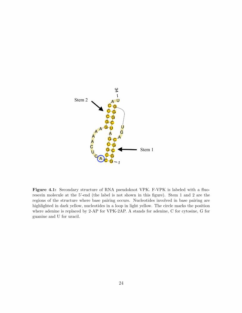
Figure 4.1 Secondary structure of RNA pseudoknot VPK. F-VPK is labeled witha fluorescein molecule at the 5’-end (the label is not shown in thisfigure). Stem 1 and 2 are the regions of the structure where basepairing occurs. Nucleotides involved in base pairing are highlightedin dark yellow, nucleotides in a loop in light yellow. The circle marksthe position where adenine is replaced by 2-AP for VPK-2AP. Astands for adenine, C for cytosine, G for guanine and U for uracil. . 24

Figure 4.2 Tertiary structure of RNA pseudoknot VPK. The residue marked bythe yellow sphere is replaced by the fluorescent nucleic acid analogue2-aminopurine (2-AP) for VPK-2AP. . . . . . . . . . . . . . . . . . 25

Figure 4.3 a) Intensity curve for F-VPK in sodium cacodylate at 30 ◦C. The plot(black dots) shows the ratio of our folding and control measurements(without counterions). The dashed line represents the ratio of thepremixing amplitudes. The fit (red line) is a single exponential decayfor the data after 200µs giving a characteristic folding time of 614 ±8µs. Before 200µs a rise can be seen, but we are unable to resolveit in terms of folding time. Apparently, the folding process startsearly and conformational changes happen already within mixing time(≈ 10µs). b) Arrhenius plot for F-VPK in MOPS. The downwardspointing triangles stand for a fitted exponential decay. The foldingrate is almost constant. . . . . . . . . . . . . . . . . . . . . . . . . . 26

vii

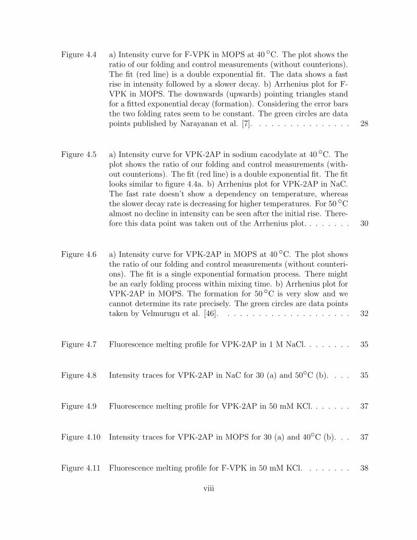
Figure 4.4 a) Intensity curve for F-VPK in MOPS at 40 ◦C. The plot shows theratio of our folding and control measurements (without counterions).The fit (red line) is a double exponential fit. The data shows a fastrise in intensity followed by a slower decay. b) Arrhenius plot for F-VPK in MOPS. The downwards (upwards) pointing triangles standfor a fitted exponential decay (formation). Considering the error barsthe two folding rates seem to be constant. The green circles are datapoints published by Narayanan et al. [7]. . . . . . . . . . . . . . . . 28

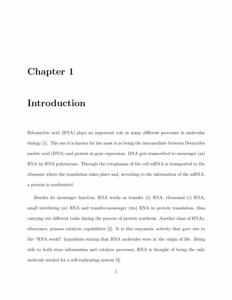
Figure 4.5 a) Intensity curve for VPK-2AP in sodium cacodylate at 40 ◦C. Theplot shows the ratio of our folding and control measurements (with-out counterions). The fit (red line) is a double exponential fit. The fitlooks similar to figure 4.4a. b) Arrhenius plot for VPK-2AP in NaC.The fast rate doesn’t show a dependency on temperature, whereasthe slower decay rate is decreasing for higher temperatures. For 50 ◦Calmost no decline in intensity can be seen after the initial rise. There-fore this data point was taken out of the Arrhenius plot. . . . . . . . 30

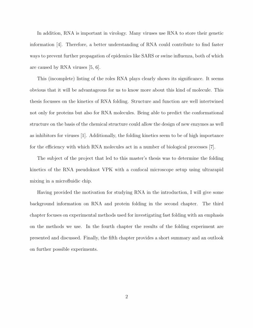
Figure 4.6 a) Intensity curve for VPK-2AP in MOPS at 40 ◦C. The plot showsthe ratio of our folding and control measurements (without counteri-ons). The fit is a single exponential formation process. There mightbe an early folding process within mixing time. b) Arrhenius plot forVPK-2AP in MOPS. The formation for 50 ◦C is very slow and wecannot determine its rate precisely. The green circles are data pointstaken by Velmurugu et al. [46]. . . . . . . . . . . . . . . . . . . . . 32

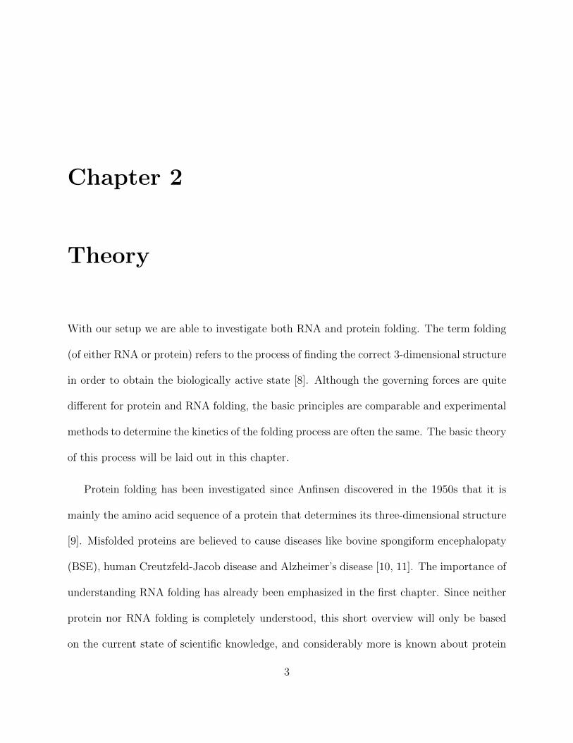
Figure 4.7 Fluorescence melting profile for VPK-2AP in 1 M NaCl. . . . . . . . 35

Figure 4.8 Intensity traces for VPK-2AP in NaC for 30 (a) and 50◦C (b). . . . 35

Figure 4.9 Fluorescence melting profile for VPK-2AP in 50 mM KCl. . . . . . . 37

Figure 4.10 Intensity traces for VPK-2AP in MOPS for 30 (a) and 40◦C (b). . . 37

Figure 4.11 Fluorescence melting profile for F-VPK in 50 mM KCl. . . . . . . . 38

viii

Figure 4.12 Intensity traces for F-VPK in MOPS for 30 (a) and 50◦C (b). . . . . 38

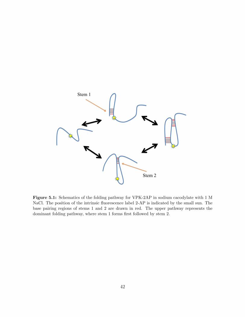
Figure 5.1 Schematics of the folding pathway for VPK-2AP in sodium cacodylatewith 1 M NaCl. The position of the intrinsic fluorescence label 2-APis indicated by the small sun. The base pairing regions of stems 1and 2 are drawn in red. The upper pathway represents the dominantfolding pathway, where stem 1 forms first followed by stem 2. . . . . 42

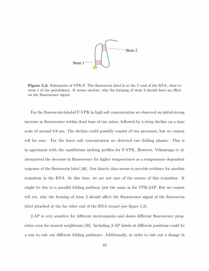
Figure 5.2 Schematics of VPK-F. The fluorescein label is at the 5’-end of theRNA, close to stem 1 of the pseudoknot. It seems unclear, why theforming of stem 2 should have an effect on the fluorescence signal. . 43

ix

Chapter 1

Introduction

Ribonucleic acid (RNA) plays an important role in many different processes in molecular

biology [1]. The one it is known for the most is as being the intermediate between Deoxyribo

nucleic acid (DNA) and protein in gene expression: DNA gets transcribed to messenger (m)

RNA by RNA polymerase. Through the cytoplasma of the cell mRNA is transported to the

ribosome where the translation takes place and, according to the information of the mRNA,

a protein is synthesized.

Besides its messenger function, RNA works as transfer (t) RNA, ribosomal (r) RNA,

small interfering (si) RNA and transfer-messenger (tm) RNA in protein translation, thus

carrying out different tasks during the process of protein synthesis. Another class of RNAs,

ribozymes, possess catalytic capabilities [2]. It is this enzymatic activity that gave rise to

the “RNA world” hypothesis stating that RNA molecules were at the origin of life. Being

able to both store information and catalyze processes, RNA is thought of being the only

molecule needed for a self-replicating system [3].

1

In addition, RNA is important in virology. Many viruses use RNA to store their genetic

information [4]. Therefore, a better understanding of RNA could contribute to find faster

ways to prevent further propagation of epidemics like SARS or swine influenza, both of which

are caused by RNA viruses [5, 6].

This (incomplete) listing of the roles RNA plays clearly shows its significance. It seems

obvious that it will be advantageous for us to know more about this kind of molecule. This

thesis focusses on the kinetics of RNA folding. Structure and function are well intertwined

not only for proteins but also for RNA molecules. Being able to predict the conformational

structure on the basis of the chemical structure could allow the design of new enzymes as well

as inhibitors for viruses [1]. Additionally, the folding kinetics seem to be of high importance

for the efficiency with which RNA molecules act in a number of biological processes [7].

The subject of the project that led to this master’s thesis was to determine the folding

kinetics of the RNA pseudoknot VPK with a confocal microscope setup using ultrarapid

mixing in a microfluidic chip.

Having provided the motivation for studying RNA in the introduction, I will give some

background information on RNA and protein folding in the second chapter. The third

chapter focuses on experimental methods used for investigating fast folding with an emphasis

on the methods we use. In the fourth chapter the results of the folding experiment are

presented and discussed. Finally, the fifth chapter provides a short summary and an outlook

on further possible experiments.

2

Chapter 2

Theory

With our setup we are able to investigate both RNA and protein folding. The term folding

(of either RNA or protein) refers to the process of finding the correct 3-dimensional structure

in order to obtain the biologically active state [8]. Although the governing forces are quite

different for protein and RNA folding, the basic principles are comparable and experimental

methods to determine the kinetics of the folding process are often the same. The basic theory

of this process will be laid out in this chapter.

Protein folding has been investigated since Anfinsen discovered in the 1950s that it is

mainly the amino acid sequence of a protein that determines its three-dimensional structure

[9]. Misfolded proteins are believed to cause diseases like bovine spongiform encephalopaty

(BSE), human Creutzfeld-Jacob disease and Alzheimer’s disease [10, 11]. The importance of

understanding RNA folding has already been emphasized in the first chapter. Since neither

protein nor RNA folding is completely understood, this short overview will only be based

on the current state of scientific knowledge, and considerably more is known about protein

3

than RNA folding.

2.1 RNA folding

RNA is built up from a sequence of four different nucleotides: adenine, cytosine, guanine

and uracil, often referred to as A, C, G and U. These nucleotides form single strands by

binding covalently to each other. Just as for DNA it is favorable for RNA to form Watson-

Crick base pairs between A and U (i.e. thymine for DNA) and C and G, respectively.

Since complimentary parts of the sequence are likely to pair, normally the RNA is not in

an extended but in a folded configuration [1]. Also, since every single nucleotide carries a

phosphate group with a negative charge, ions in the solvent play an important role for the

folding process [12].

The sequence information is referred to as the primary structure. Secondary structure

describes the Watson-Crick base pairs that form as a consequence of available hydrogen

bonds, base stacking and electrostatic interactions. Double stranded RNA forms double

helices just as DNA does. The secondary structure motifs RNA can form are hairpins,

bulges, internal loops and junctions. Finally, tertiary structure characterizes how secondary

structures orient with respect to each other. The RNA we investigated for this thesis forms

a pseudoknot. This is essentially a hairpin loop that base-pairs with a later part of the

sequence. Other tertiary structures include for example loop-loop interactions [13].

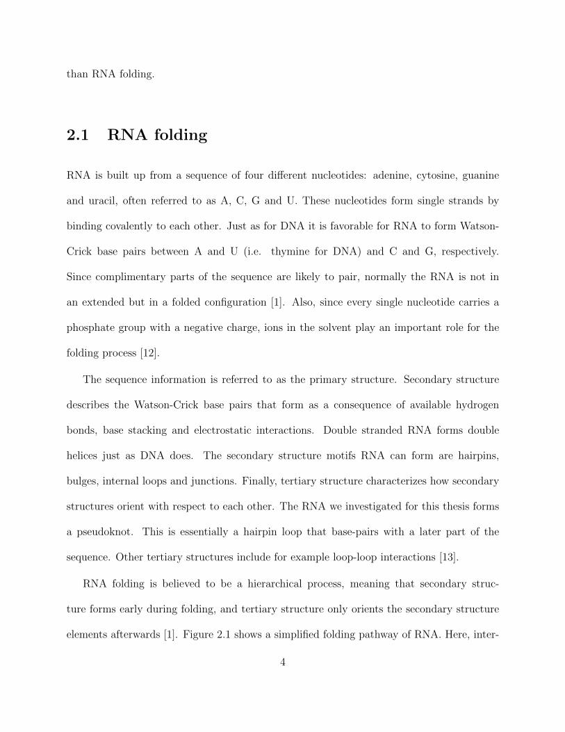
RNA folding is believed to be a hierarchical process, meaning that secondary struc-

ture forms early during folding, and tertiary structure only orients the secondary structure

elements afterwards [1]. Figure 2.1 shows a simplified folding pathway of RNA. Here, inter-

4

ΔG

Folding reaction

U

I

F

Figure 2.1: Simplified view of a folding reaction. The unfolded state (U) is energeticallyunfavourable. The native, i.e. folded state (F) minimizes ∆G. During the folding process themolecule can get trapped in (multiple) local minima of the energy landscape. These conforma-tions are called intermediate states (I). For interpretation of the references to color in this andall other figures, the reader is referred to the electronic version of this thesis.

mediate states (commonly referred to as I or IS), that could trap the RNA in a non-native

state, may show up.

2.2 Folding kinetics

Perhaps the easiest way the folding process can be thought of is a transition within a two-

state model. This approach is valid under the condition of rapid equilibration of the unfolded

conformations before folding takes place [14]. The two-state model has a denatured or

unfolded (U) state and a native or folded (F) state. These two states are in equilibrium

5

with each other and knowing the folding and unfolding rates kf and ku, we can calculate

the equilibrium constant Keq and the difference in the Gibbs free energy, ∆G, which is a

measure of the stability of the folded protein [15]:

Fkukf

U (2.1)

Keq =kukf

(2.2)

∆Gunfold = −RT lnKeq (2.3)

with R the universal gas constant and T the absolute temperature. ∆G can also be written

as:

∆Gunfold = ∆H − T∆S (2.4)

with ∆H and ∆S the change in enthalpy and entropy, respectively. Equation 2.4 elucidates

that folding is an interplay between entropy and enthalpy. When a protein folds, the number

of possible configurations is reduced, i.e. S decreases unfavorably. Therefore folding can only

occur when at the same time enthalpy decreases by the forming of energetically favorable

contacts between nucleotides [16].

In terms of folding time τf , equation 2.3 can be written as:

τf = τ0f · exp

(∆GFkBT

)(2.5)

where ∆GF is the height of the free energy barrier and τ0f a prefactor which can be approx-

6

ΔG

U

F

ΔG

ΔG

ΔG unfold

F

U

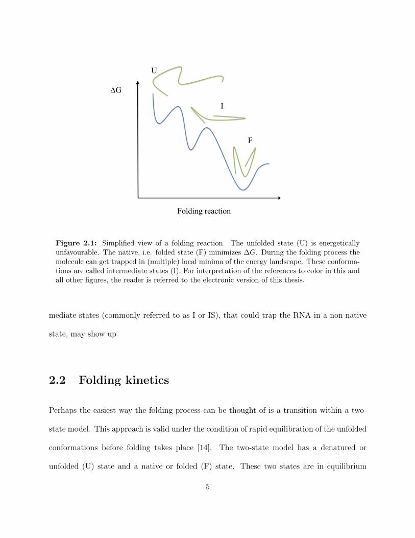
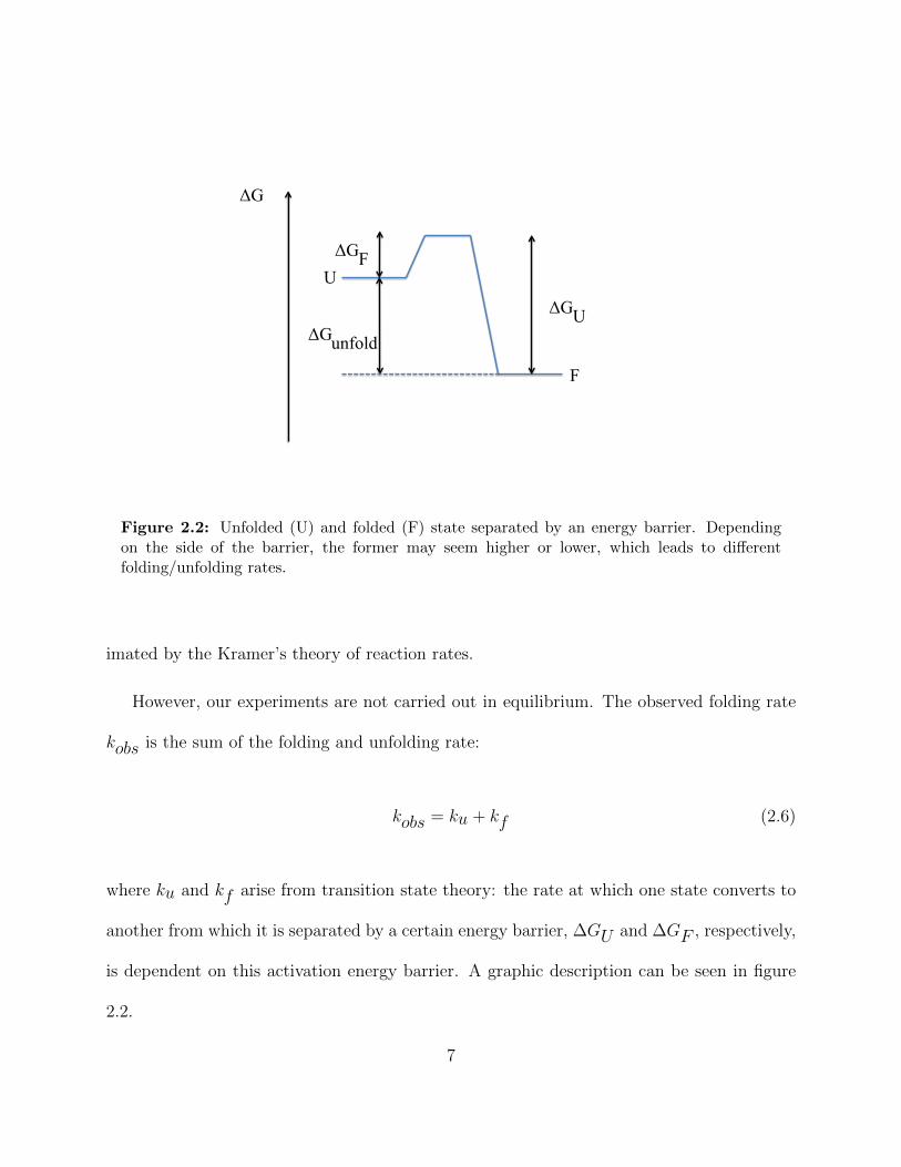
Figure 2.2: Unfolded (U) and folded (F) state separated by an energy barrier. Dependingon the side of the barrier, the former may seem higher or lower, which leads to differentfolding/unfolding rates.

imated by the Kramer’s theory of reaction rates.

However, our experiments are not carried out in equilibrium. The observed folding rate

kobs is the sum of the folding and unfolding rate:

kobs = ku + kf (2.6)

where ku and kf arise from transition state theory: the rate at which one state converts to

another from which it is separated by a certain energy barrier, ∆GU and ∆GF , respectively,

is dependent on this activation energy barrier. A graphic description can be seen in figure

2.2.

7

ln k

[Denaturant/salt]

k k U F

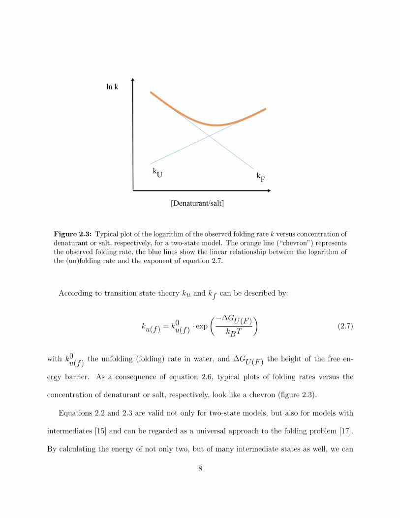
Figure 2.3: Typical plot of the logarithm of the observed folding rate k versus concentration ofdenaturant or salt, respectively, for a two-state model. The orange line (“chevron”) representsthe observed folding rate, the blue lines show the linear relationship between the logarithm ofthe (un)folding rate and the exponent of equation 2.7.

According to transition state theory ku and kf can be described by:

ku(f) = k0u(f) · exp

(−∆GU(F )

kBT

)(2.7)

with k0u(f)

the unfolding (folding) rate in water, and ∆GU(F ) the height of the free en-

ergy barrier. As a consequence of equation 2.6, typical plots of folding rates versus the

concentration of denaturant or salt, respectively, look like a chevron (figure 2.3).

Equations 2.2 and 2.3 are valid not only for two-state models, but also for models with

intermediates [15] and can be regarded as a universal approach to the folding problem [17].

By calculating the energy of not only two, but of many intermediate states as well, we can

8

draw an energy landscape. This energy landscape is like a rugged funnel through which RNA

or protein has to go upon folding and in which it sometimes gets trapped in intermediate

states. Rather than being well-defined, intermediate states often resemble an ensemble of

states [18]. Beauchamp et al. recently investigated whether the two-state model describes

protein folding well [19]. Based on 14 different protein folding simulations their conclusion

is that the two-state model is a reasonable approximation of the folding process.

2.3 Protein folding

All the equations in the last section hold for RNA and protein folding. Only the governing

principles are different, since the structures of RNAs and proteins differ.

The primary structure of proteins is a sequence of 20 different amino acids. As opposed to

RNA, some amino acids carry either a positive or a negative charge, and some are electrically

neutral. Proteins consist of from a few tens to thousands of amino acids. The protein titin,

for example, is made up of around 30,000 amino acids [20]. Amino acids not adjacent in the

sequence interact with each other via hydrogen bonds and electrostatic interactions. This and

the hydrophobicity of some of the amino acids leads to the forming the secondary structure.

The most common motifs are α-helices, β-sheets and connecting loops [8]. Tertiary structure,

again, is the spatial orientation of these secondary structure elements.

9

2.4 Computational approaches to RNA and protein

folding

Soon after the structure of proteins was discovered the so called Levinthal Paradox became

apparent [21]: The molecules find their unique structure in a much shorter time than needed

for an entropic search through all possible conformations. Despite advances it still remains

most challenging to simulate the folding process. Simulating 1 nanosecond still takes around

one day for a supercomputer [22].

Progress has been achieved by both new algorithms and better hardware. New tech-

niques and better algorithms, e.g. more exact force fields and coarse-grained models, speed

up the simulation of protein folding. Recently Lindorff-Larsen et. al. published a study

showing their results of all-atom molecular dynamics (MD) simulations for 12 different pro-

tein domains and comparing them in a consistent way [23]. These simulations were run

on a specifically designed parallel supercomputer called “Anton” [24]. The project “Fold-

ing@home” follows a distributed computing approach that uses idle time of participating

personal computers to obtain more and more computational power [25]. Therefore all-atom

MD simulations for large proteins might be feasible in a reasonable amount of time not too

far away in the future [26].

However, since the big breakthrough in understanding protein folding has not occurred

yet, further experiments are still necessary, not least for the validation of computational

results.

10

2.5 Experimental approaches to RNA and protein fold-

ing

RNA and protein folding is still a huge challenge to investigate and also to computationally

simulate. In order to reduce complexity fast-folding proteins with folding times shorter than

100µs have become the focus of attention [27]. In general folding can be initialized by chain

synthesis, the application of forces to the ends of the molecule or by changing the chemical

environment, i.e. the solvent [28]. For fast-folding experiments the latter is the preferred

method. There are different ways to change the solvent condition, e.g. photochemical

triggering, temperature- or pressure-jump, and ultrarapid mixing [29]. For our experiments

described in this thesis we used ultrarapid mixing and later on we will compare our results

with temperature (T)-jump experiments. Both of these methods will be described in chapters

3.2 and 3.4, respectively.

11

Chapter 3

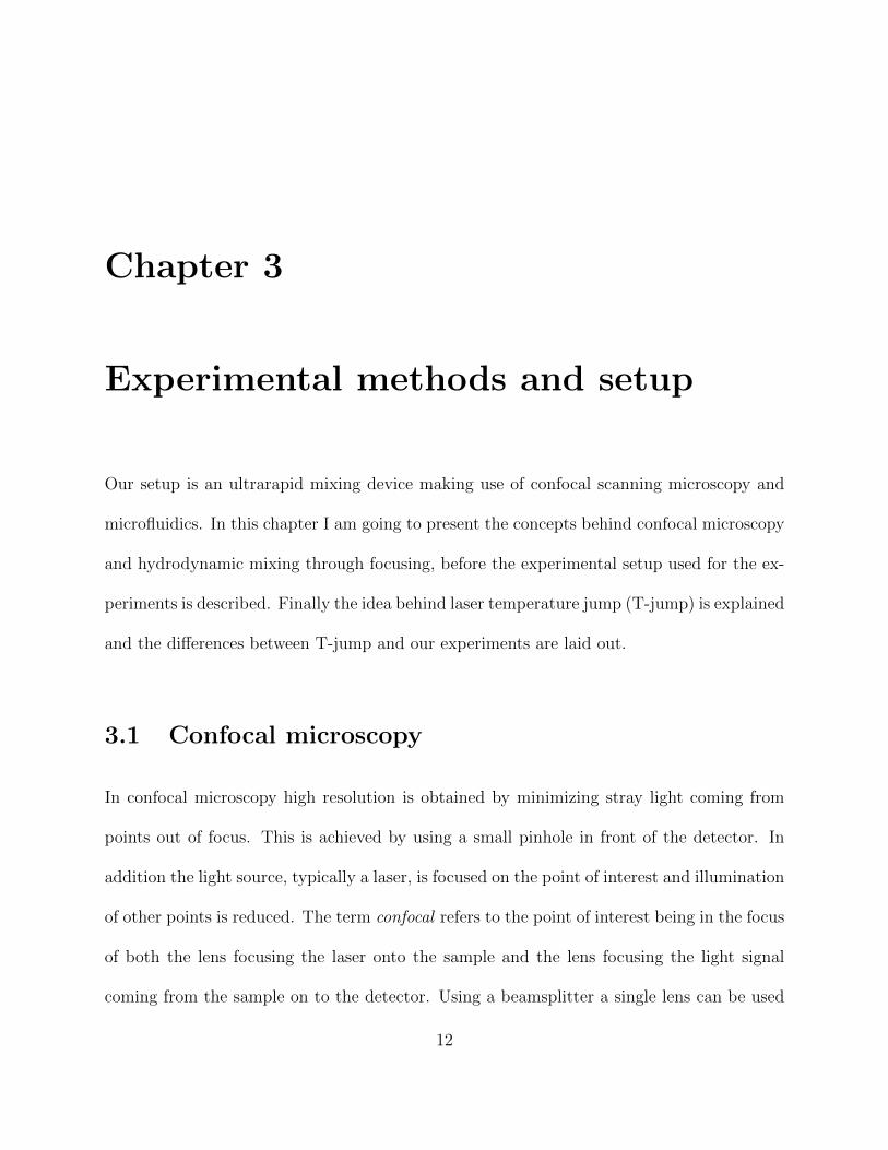
Experimental methods and setup

Our setup is an ultrarapid mixing device making use of confocal scanning microscopy and

microfluidics. In this chapter I am going to present the concepts behind confocal microscopy

and hydrodynamic mixing through focusing, before the experimental setup used for the ex-

periments is described. Finally the idea behind laser temperature jump (T-jump) is explained

and the differences between T-jump and our experiments are laid out.

3.1 Confocal microscopy

In confocal microscopy high resolution is obtained by minimizing stray light coming from

points out of focus. This is achieved by using a small pinhole in front of the detector. In

addition the light source, typically a laser, is focused on the point of interest and illumination

of other points is reduced. The term confocal refers to the point of interest being in the focus

of both the lens focusing the laser onto the sample and the lens focusing the light signal

coming from the sample on to the detector. Using a beamsplitter a single lens can be used

12

Figure 3.1: Schematics of epitaxial confocal microscopy. Point illumination excites onlyfluorophores in the focal volume. Stray light from points out of focus (orange line) is blockedby a pinhole. These two measures increase the signal-to-noise ratio significantly.

for both purposes as it is shown in figure 3.1. This is called epitaxial confocal microscopy,

since light source and detector are on the same side of the sample [30].

Theoretically the resolution R of a diffraction limited microscope is given by the Rayleigh

criterion [31]:

R =0.61 · λNA

(3.1)

where λ is the wavelength of the illuminating light and NA the numerical aperture. This

limit is referring to the case where the first diffraction minimum of one source point coincides

with the maximum of another.

Confocal microscopes have a slightly higher resolution due to only pointwise illumination

13

of the sample. The theoretical resolution then is approximately [32]:

Rconfocal =0.4 · λNA

(3.2)

For our argon ion laser at λ = 258 nm and a numerical aperture of 0.5, as used in our

experiment, this results in an optical resolution of R ≈ 200 nm = 0.2µm. Even so, the

manufacturer of the objective used in our setup states a maximum resolution of only 1µm.

3.2 Microfluidic mixing

Mixing is most often associated with turbulence. In order to achieve shorter mixing times,

however, turbulent mixing it is not necessarily the best way [33]. Hydrodynamic focusing in

microfluidic devices uses the laminar flow regime to mix solutions quickly and in a controlled

manner.

A way to differentiate between turbulent and laminar flow is the Reynolds number. It is

defined as the ratio between viscous and inertial forces and, for a flow it can be simplified

to [34]:

Re =u ·Dhν

(3.3)

where u is the velocity, ν the kinematic viscosity and Dh is the hydraulic diameter. The

latter is essentially the diameter of the passage. For Reynolds numbers lower than 100 the

flow is laminar, the transition to turbulent flow occurs at around Re ≈ 2000 [35]. Therefore

using very small channel dimensions allows work in the laminar flow regime. Applying

equation 3.3 to our setup, for a kinematic viscosity of around 10−6 m/s2 for water at room

14

temperature, a typical flow speed of 1 m/s and channel dimensions of 10 µm, the Reynolds

number equals 10. Therefore the flow conditions in our microfluidic chip are well in the

laminar flow regime.

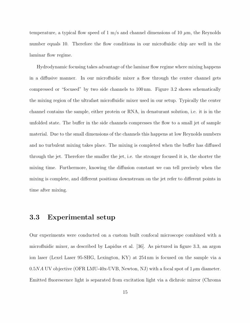
Hydrodynamic focusing takes advantage of the laminar flow regime where mixing happens

in a diffusive manner. In our microfluidic mixer a flow through the center channel gets

compressed or “focused” by two side channels to 100 nm. Figure 3.2 shows schematically

the mixing region of the ultrafast microfluidic mixer used in our setup. Typically the center

channel contains the sample, either protein or RNA, in denaturant solution, i.e. it is in the

unfolded state. The buffer in the side channels compresses the flow to a small jet of sample

material. Due to the small dimensions of the channels this happens at low Reynolds numbers

and no turbulent mixing takes place. The mixing is completed when the buffer has diffused

through the jet. Therefore the smaller the jet, i.e. the stronger focused it is, the shorter the

mixing time. Furthermore, knowing the diffusion constant we can tell precisely when the

mixing is complete, and different positions downstream on the jet refer to different points in

time after mixing.

3.3 Experimental setup

Our experiments were conducted on a custom built confocal microscope combined with a

microfluidic mixer, as described by Lapidus et al. [36]. As pictured in figure 3.3, an argon

ion laser (Lexel Laser 95-SHG, Lexington, KY) at 254 nm is focused on the sample via a

0.5NA UV objective (OFR LMU-40x-UVB, Newton, NJ) with a focal spot of 1µm diameter.

Emitted fluorescence light is separated from excitation light via a dichroic mirror (Chroma

15

Buffer

Buffer

RNA/Protein in Denaturant Solution

Figure 3.2: Schematics of our mixing chip. Flow through the center channel containingRNA/protein in denaturant solution gets compressed (“focused”) by two side channels con-taining buffer, and a jet of center channel solution is formed. Sandwiched by buffer theRNA/protein solution flows down the mixing channel. Buffer diffuses quickly into the tinyjet, and different positions behind the mixing region can be assigned different points in timeafter mixing, thus allowing a time resolved investigation of the folding kinetics.

16

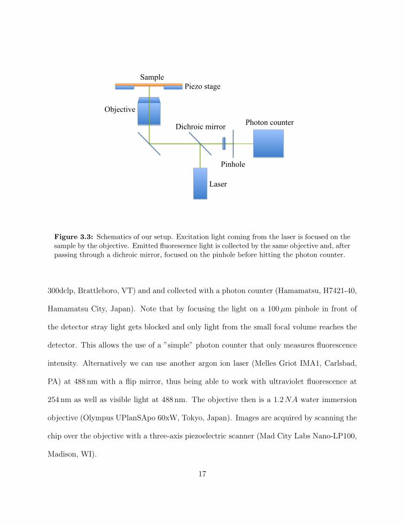
Photon counter

Laser

Dichroic mirror

Objective

Piezo stage Sample

Pinhole

Figure 3.3: Schematics of our setup. Excitation light coming from the laser is focused on thesample by the objective. Emitted fluorescence light is collected by the same objective and, afterpassing through a dichroic mirror, focused on the pinhole before hitting the photon counter.

300dclp, Brattleboro, VT) and and collected with a photon counter (Hamamatsu, H7421-40,

Hamamatsu City, Japan). Note that by focusing the light on a 100µm pinhole in front of

the detector stray light gets blocked and only light from the small focal volume reaches the

detector. This allows the use of a ”simple” photon counter that only measures fluorescence

intensity. Alternatively we can use another argon ion laser (Melles Griot IMA1, Carlsbad,

PA) at 488 nm with a flip mirror, thus being able to work with ultraviolet fluorescence at

254 nm as well as visible light at 488 nm. The objective then is a 1.2NA water immersion

objective (Olympus UPlanSApo 60xW, Tokyo, Japan). Images are acquired by scanning the

chip over the objective with a three-axis piezoelectric scanner (Mad City Labs Nano-LP100,

Madison, WI).

17

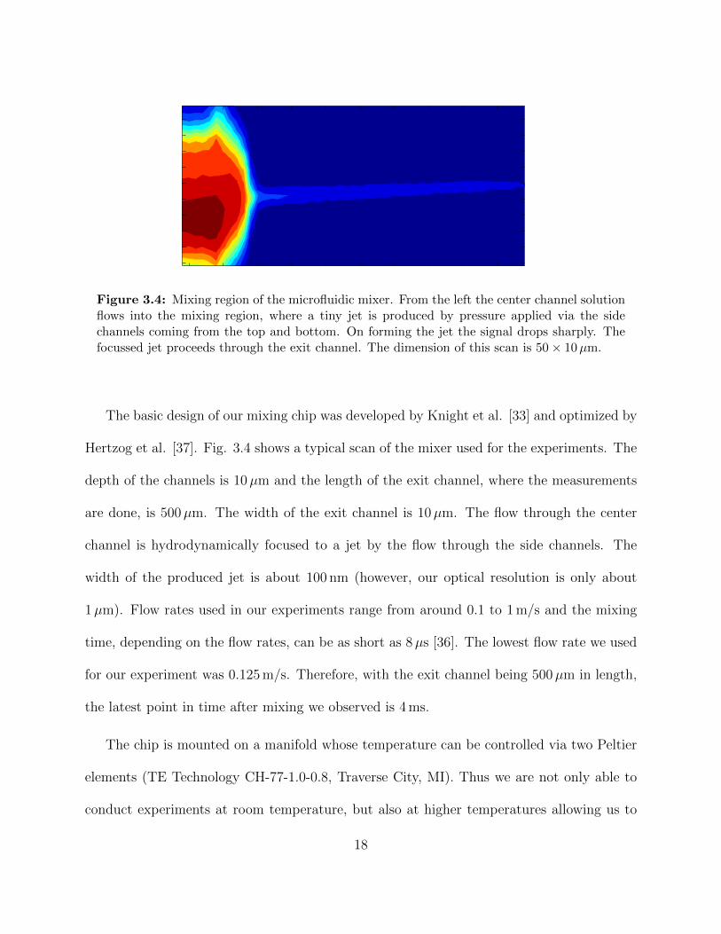
Figure 3.4: Mixing region of the microfluidic mixer. From the left the center channel solutionflows into the mixing region, where a tiny jet is produced by pressure applied via the sidechannels coming from the top and bottom. On forming the jet the signal drops sharply. Thefocussed jet proceeds through the exit channel. The dimension of this scan is 50 × 10µm.

The basic design of our mixing chip was developed by Knight et al. [33] and optimized by

Hertzog et al. [37]. Fig. 3.4 shows a typical scan of the mixer used for the experiments. The

depth of the channels is 10µm and the length of the exit channel, where the measurements

are done, is 500µm. The width of the exit channel is 10µm. The flow through the center

channel is hydrodynamically focused to a jet by the flow through the side channels. The

width of the produced jet is about 100 nm (however, our optical resolution is only about

1µm). Flow rates used in our experiments range from around 0.1 to 1 m/s and the mixing

time, depending on the flow rates, can be as short as 8µs [36]. The lowest flow rate we used

for our experiment was 0.125 m/s. Therefore, with the exit channel being 500µm in length,

the latest point in time after mixing we observed is 4 ms.

The chip is mounted on a manifold whose temperature can be controlled via two Peltier

elements (TE Technology CH-77-1.0-0.8, Traverse City, MI). Thus we are not only able to

conduct experiments at room temperature, but also at higher temperatures allowing us to

18

reach different regions of the energy landscape of the folding process. The manifold also

incorporates reservoirs for the different solutions. Computer controlled pressure transducers

(Marsh Bellofram Type 2000, Newell, WV) apply air pressure on these reservoirs in order to

obtain the desired flow speeds.

Folding can be observed as a change in fluorescent signal from the jet. The molecules

under observation are either intrinsically fluorescent or have some fluorescent labels attached.

In certain structural conformations quenching occurs, i.e. quantum yield, and therefore

fluorescent intensity decreases. This allows to deduce in which conformational state, folded

or unfolded, the molecules are. Most important to us, even if we don’t know the exact

configuration, the change in signal intensity tells us about the kinetics of the folding reaction.

In order to differentiate between loss in fluorescence intensity due to diffusion out of the

jet and due to a change in conformation, respectively, we have to take control measurements

without the salt in the side channels. We then analyze the ratio of the intensities from

the folding and control measurements along the jet. This ratio should reveal characteristic

folding kinetics by comparing it with equilibrium fluorescence data. Another advantage of

taking the ratio is to overcome the signal drop in the mixing region due to the forming the

jet (cf. figure 3.4).

3.4 Temperature jump

Laser temperature jump (T-jump) is a method that investigates kinetic processes of biolog-

ical macromolecules. Starting from equilibrium a system gets disturbed by a rapid rise in

temperature. This disturbance is most often a short laser pulse that heats up the sample. In

19

order to gain a high temporal resolution, the laser pulse has to be short. However, it should

be powerful enough to change the equilibrated system significantly. After the pulse the re-

laxation of the system can be monitored, e.g. by UV absorption or fluorescence intensity.

Because of the high temporal resolution of this technique it is very well suited for ultra-fast

folding molecules [38].

3.5 Difference in T- and ion-jump experiments

T- and ion-jump experiments both investigate the kinetics from a non-native to the native

state. However, the trigger for starting this transition differs for the two methods. In T-jump

experiments a sudden change in temperature disturbs an equilibrated system. The deviation

from the equilibrium by the T-jump is dependent on the change in temperature. Speaking

in terms of an energy landscape for folding processes, the bigger the jump, the farther away

the system gets from its original state.

Our setup is an ion-jump experiment. Ultrarapid mixing represents an abrupt change in

solvent environment for the RNA. After mixing the system is observed while it is equilibrat-

ing. Since the sample is first in denaturant without salt, it is completely unfolded and in an

extended conformation due to its intrinsic negative charges.

This difference in starting conditions for the two methods is crucial. Biyun et al. studied

the difference of the two methods in a coarse grained molecular dynamics simulation of a

pseudoknot found in human telomerase [39]. For ion-jump experiments electrostatic inter-

actions lead to a very fast folding process at timescales of a few hundred microseconds. On

the other hand, for T-jump experiments non-bonded tertiary interactions, which are weaker

20

compared to electrostatic interactions, play a major role. One of the results of their sim-

ulation is that folding after ion-jump usually happens faster than after T-jump. In their

specific case of the human telomerase RNA pseudoknot, the first phase of folding happened

five times faster for ion jump than for T-jump, and the slower phase took only half the time.

However, Narayanan et al. recently reported folding/unfolding kinetics of a nucleic acid

hairpin investigated by both laser T-jump and ion-jump (ultrafast mixing with counterions),

with folding rates for ion-jump as much as 10 times slower than for T-jump [40]. This might

be due to the fact that in ion-jump experiments nucleic acids collapses very quickly and the

subsequent kinetics are mainly dominated by a transition from the collapsed to the folded

state.

21

Chapter 4

Folding kinetics of RNA pseudoknot

VPK

In general, pseudoknots as a minimal motif in secondary structure of RNA play a crucial

role in many biological processes, such as translational frameshifting and gene expression

and replication [7, 41, 42]. As mentioned earlier, small, fast-folding molecules are interesting

objects to study due to their lower complexity. The folding process is less complicated and

easier to reconstruct. The following chapter presents the results of our experiments on the

folding kinetics of RNA pseudoknot VPK, which is a variant of the mouse mammary tumor

virus (MMTV) mRNA.

4.1 Experimental details

The setup we used for the experiments was described in chapter 3.3. We conducted experi-

ments with two different samples. One was pseudoknot F-VPK labeled with fluorescein at the

22

5’-end. The other one was VPK-2AP with one nucleic acid substituted with 2-aminopurine

(2-AP). 2-AP is a fluorescent analog of adenine and guanine, allowing to investigate the

structure and kinetics of RNA and DNA, respectively [43]. In our sample, a gift from the

Ansari group at the University of Illinois at Chicago, only a single adenine base is replaced

by 2-AP (cf. figure 4.1). These two samples highlight slightly different features of the folding

process, since the fluorescence signal comes from different positions in the secondary struc-

ture: the fluorescein label is attached at one end of the pseudoknot, 2-AP is at position 20

of the RNA chain. Although the fluorescence signal under folding might look different for

the two samples, the derived kinetics from both samples should be the same if the relatively

large fluorescein label has no impact on the folding process.

For the experiments, both samples were dissolved in 8 M urea, a strong denaturant. Urea

prohibits hydrogen bonding between RNA strands, i.e. the forming of secondary structure,

by making hydrogen bonds with the RNA bases itself [44]. Therefore, before mixing the

RNA in the center channel is in an unfolded, extended conformation, not least because no

counterions are present in order to prevent the nucleotides from repelling each other due to

their negative charge.

The side channels contained either 10 mM sodium cacodylate (NaC) with 1 M sodium

chloride (NaCl) or 10 mM 3-(N-morpholino)propanesulfonic acid (MOPS) buffer with 50 mM

potassium chloride (KCl), from now on referred to as NaC and MOPS, respectively. These

two different folding environments allow us to compare our results with recently published

papers [7, 45]. The low salt concentration in MOPS is a more physiological environment,

the high salt concentration in sodium cacodylate buffer is closer to the simulated conditions

by Cho et al. [45]. The salt in the side channels provides a charged environment. These

23

Stem 1

Stem 2

Figure 4.1: Secondary structure of RNA pseudoknot VPK. F-VPK is labeled with a fluo-rescein molecule at the 5’-end (the label is not shown in this figure). Stem 1 and 2 are theregions of the structure where base pairing occurs. Nucleotides involved in base pairing arehighlighted in dark yellow, nucleotides in a loop in light yellow. The circle marks the positionwhere adenine is replaced by 2-AP for VPK-2AP. A stands for adenine, C for cytosine, G forguanine and U for uracil.

24

Figure 4.2: Tertiary structure of RNA pseudoknot VPK. The residue marked by the yellowsphere is replaced by the fluorescent nucleic acid analogue 2-aminopurine (2-AP) for VPK-2AP.

counterions are crucial for the RNA to fold, since all the single nucleic acids are negatively

charged and would repel each other otherwise.

Briefly, we mix unfolded RNA in folding buffer and observe the folding process.

4.2 Results

We investigated folding kinetics for the two slightly different samples (F-VPK and VPK-

2AP) and two folding conditions (NaC and MOPS) at up to 7 different temperatures.

A typical fluorescence intensity curve for F-VPK in NaC is shown in figure 4.3a. It shows

a steep rise shortly after mixing and a slower decay afterwards. We normalized the data,

so that for t < 0, i.e. before mixing, the intensity ratio of control and folding experiments

is 1. The fact that the intensity ratio shortly after mixing is constantly above 1 for all

measurements, is a clear sign for an early folding process within and shortly after our mixing

25

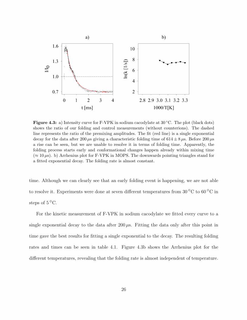
Figure 4.3: a) Intensity curve for F-VPK in sodium cacodylate at 30 ◦C. The plot (black dots)shows the ratio of our folding and control measurements (without counterions). The dashedline represents the ratio of the premixing amplitudes. The fit (red line) is a single exponentialdecay for the data after 200µs giving a characteristic folding time of 614 ± 8µs. Before 200µsa rise can be seen, but we are unable to resolve it in terms of folding time. Apparently, thefolding process starts early and conformational changes happen already within mixing time(≈ 10µs). b) Arrhenius plot for F-VPK in MOPS. The downwards pointing triangles stand fora fitted exponential decay. The folding rate is almost constant.

time. Although we can clearly see that an early folding event is happening, we are not able

to resolve it. Experiments were done at seven different temperatures from 30 ◦C to 60 ◦C in

steps of 5 ◦C.

For the kinetic measurement of F-VPK in sodium cacodylate we fitted every curve to a

single exponential decay to the data after 200µs. Fitting the data only after this point in

time gave the best results for fitting a single exponential to the decay. The resulting folding

rates and times can be seen in table 4.1. Figure 4.3b shows the Arrhenius plot for the

different temperatures, revealing that the folding rate is almost independent of temperature.

26

Table 4.1: Folding rates and times for F-VPK in NaC based on a single exponential fitexcluding data points before 200µs.

T in ◦C k in 1/s ∆k in 1/s τf in s ∆τ in s

30 1630 20 6.15E-04 7.E-0635 1990 20 5.02E-04 5.E-0640 1700 20 5.89E-04 7.E-0645 1650 30 6.07E-04 9.E-0650 1210 20 8.3E-04 2.E-0555 1750 30 5.70E-04 9.E-0660 2530 50 3.95E-04 7.E-06

27

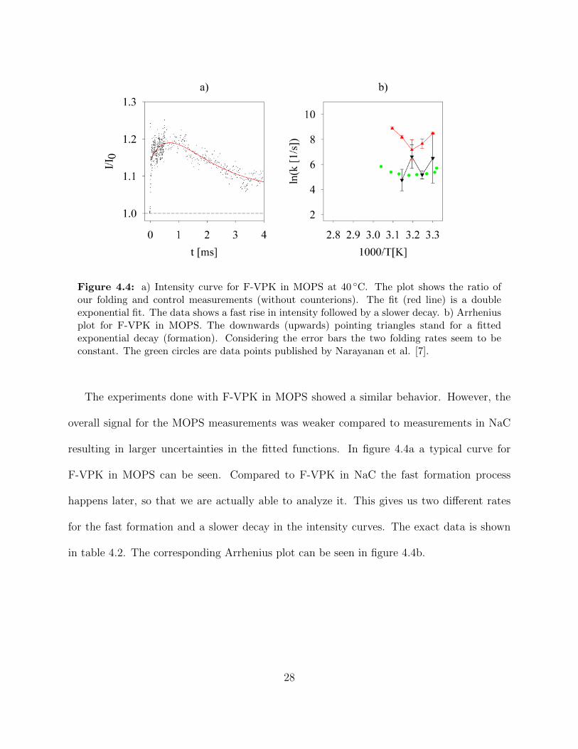
Figure 4.4: a) Intensity curve for F-VPK in MOPS at 40 ◦C. The plot shows the ratio ofour folding and control measurements (without counterions). The fit (red line) is a doubleexponential fit. The data shows a fast rise in intensity followed by a slower decay. b) Arrheniusplot for F-VPK in MOPS. The downwards (upwards) pointing triangles stand for a fittedexponential decay (formation). Considering the error bars the two folding rates seem to beconstant. The green circles are data points published by Narayanan et al. [7].

The experiments done with F-VPK in MOPS showed a similar behavior. However, the

overall signal for the MOPS measurements was weaker compared to measurements in NaC

resulting in larger uncertainties in the fitted functions. In figure 4.4a a typical curve for

F-VPK in MOPS can be seen. Compared to F-VPK in NaC the fast formation process

happens later, so that we are actually able to analyze it. This gives us two different rates

for the fast formation and a slower decay in the intensity curves. The exact data is shown

in table 4.2. The corresponding Arrhenius plot can be seen in figure 4.4b.

28

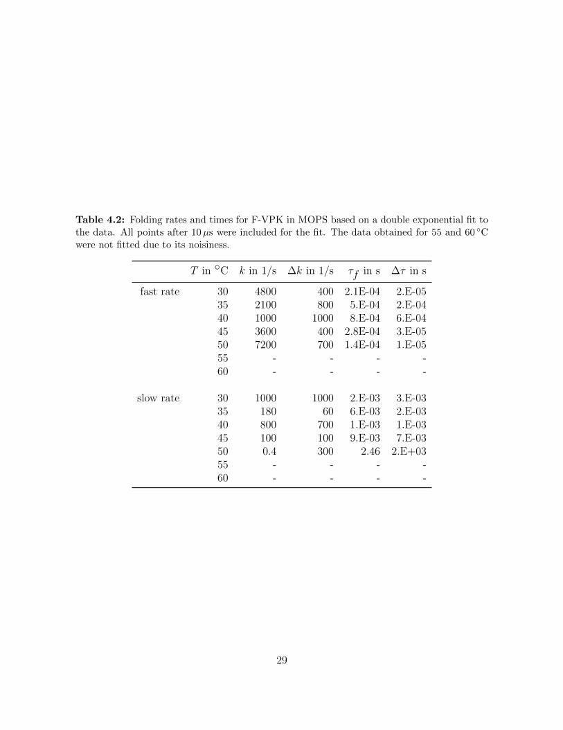
Table 4.2: Folding rates and times for F-VPK in MOPS based on a double exponential fit tothe data. All points after 10µs were included for the fit. The data obtained for 55 and 60 ◦Cwere not fitted due to its noisiness.

T in ◦C k in 1/s ∆k in 1/s τf in s ∆τ in s

fast rate 30 4800 400 2.1E-04 2.E-0535 2100 800 5.E-04 2.E-0440 1000 1000 8.E-04 6.E-0445 3600 400 2.8E-04 3.E-0550 7200 700 1.4E-04 1.E-0555 - - - -60 - - - -

slow rate 30 1000 1000 2.E-03 3.E-0335 180 60 6.E-03 2.E-0340 800 700 1.E-03 1.E-0345 100 100 9.E-03 7.E-0350 0.4 300 2.46 2.E+0355 - - - -60 - - - -

29

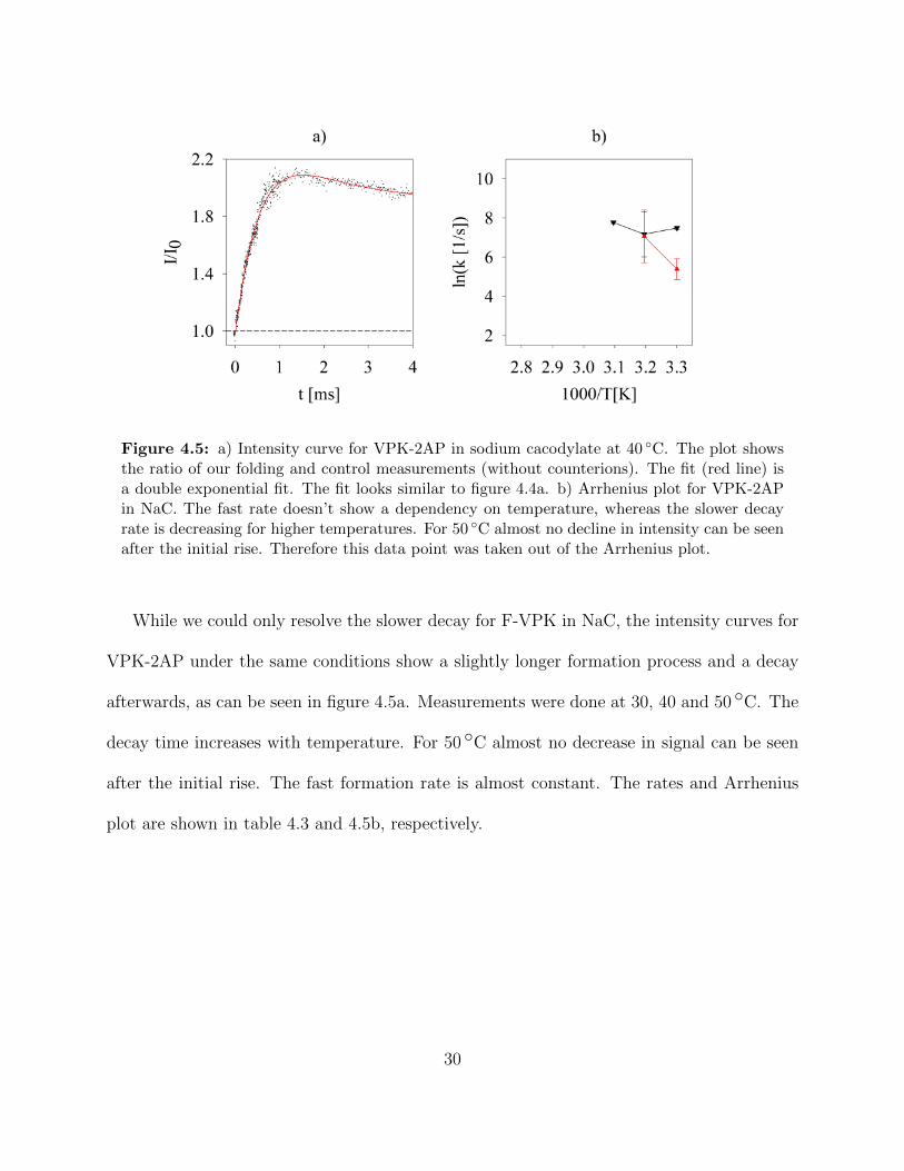
Figure 4.5: a) Intensity curve for VPK-2AP in sodium cacodylate at 40 ◦C. The plot showsthe ratio of our folding and control measurements (without counterions). The fit (red line) isa double exponential fit. The fit looks similar to figure 4.4a. b) Arrhenius plot for VPK-2APin NaC. The fast rate doesn’t show a dependency on temperature, whereas the slower decayrate is decreasing for higher temperatures. For 50 ◦C almost no decline in intensity can be seenafter the initial rise. Therefore this data point was taken out of the Arrhenius plot.

While we could only resolve the slower decay for F-VPK in NaC, the intensity curves for

VPK-2AP under the same conditions show a slightly longer formation process and a decay

afterwards, as can be seen in figure 4.5a. Measurements were done at 30, 40 and 50 ◦C. The

decay time increases with temperature. For 50 ◦C almost no decrease in signal can be seen

after the initial rise. The fast formation rate is almost constant. The rates and Arrhenius

plot are shown in table 4.3 and 4.5b, respectively.

30

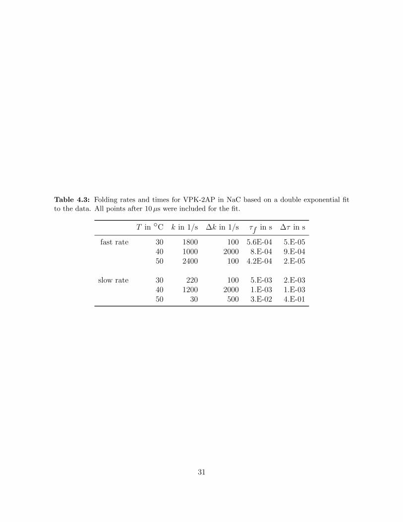
Table 4.3: Folding rates and times for VPK-2AP in NaC based on a double exponential fitto the data. All points after 10µs were included for the fit.

T in ◦C k in 1/s ∆k in 1/s τf in s ∆τ in s

fast rate 30 1800 100 5.6E-04 5.E-0540 1000 2000 8.E-04 9.E-0450 2400 100 4.2E-04 2.E-05

slow rate 30 220 100 5.E-03 2.E-0340 1200 2000 1.E-03 1.E-0350 30 500 3.E-02 4.E-01

31

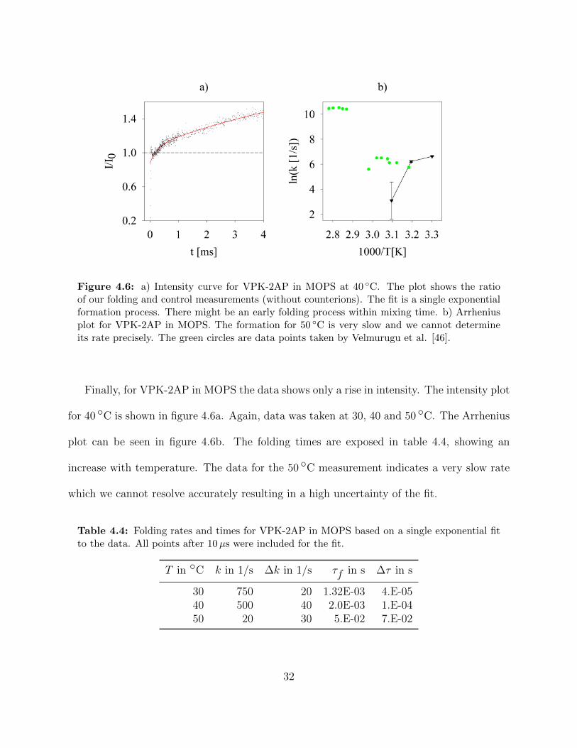
Figure 4.6: a) Intensity curve for VPK-2AP in MOPS at 40 ◦C. The plot shows the ratioof our folding and control measurements (without counterions). The fit is a single exponentialformation process. There might be an early folding process within mixing time. b) Arrheniusplot for VPK-2AP in MOPS. The formation for 50 ◦C is very slow and we cannot determineits rate precisely. The green circles are data points taken by Velmurugu et al. [46].

Finally, for VPK-2AP in MOPS the data shows only a rise in intensity. The intensity plot

for 40 ◦C is shown in figure 4.6a. Again, data was taken at 30, 40 and 50 ◦C. The Arrhenius

plot can be seen in figure 4.6b. The folding times are exposed in table 4.4, showing an

increase with temperature. The data for the 50 ◦C measurement indicates a very slow rate

which we cannot resolve accurately resulting in a high uncertainty of the fit.

Table 4.4: Folding rates and times for VPK-2AP in MOPS based on a single exponential fitto the data. All points after 10µs were included for the fit.

T in ◦C k in 1/s ∆k in 1/s τf in s ∆τ in s

30 750 20 1.32E-03 4.E-0540 500 40 2.0E-03 1.E-0450 20 30 5.E-02 7.E-02

32

4.3 Discussion

The folding kinetics of RNA pseudoknot VPK have been investigated recently by two other

groups. Cho et al. simulated the folding process of VPK in a coarse grained molecular

dynamics simulation [45]. In their simulation they generated an ensemble of unfolded con-

formations at a temperature above the highest melting temperature. Folding is triggered

by suddenly reducing the temperature in the simulation to a level below the lowest melt-

ing temperature. They reported a hierarchical mechanism with parallel folding pathways.

The formation of one loop initiates the folding process. VPK has two stems with distinct

stabilities. In terms of free energy stem 1 (cf. figure 4.1) is about 3.8 kcal/mol more stable

than stem 2, resulting in a dominating pathway where stem 1 forms before stem 2 with a

probability of 77 %. Corresponding to these different stabilities Cho et al. determined the

folding time for stem 1 and stem 2 to be about 0.4 ms and 4.3 ms, respectively [45].

Recently Narayanan et al. confirmed these theoretical predictions in a T-jump experiment

[7]. They measured folding times of about 0.95 ms and 4.3 ms. This is in very good agreement

with the simulation data. As discussed in chapter 3.5, theoretically slightly shorter folding

times for ion-jump experiments compared to T-jump are predicted; experimentally, however,

the opposite was shown.

Our folding conditions were chosen so as to be able to compare our results with the

aforementioned studies. However, a direct comparison between the experiments in 10 mM

MOPS with 50 mM KCl and 10 mM NaC with 1 M NaCl might not be possible. Vieregg

et al. measured a slight difference in RNA hairpin stability and folding rate depending on

whether potassium or sodium cations were present [47].

33

While for all of our experiments, except for VPK-2AP in MOPS, we could see at least

two kinetic phases, we were not able to resolve all of them properly. This was partly because

the corresponding folding event started already within the dead time of our mixer, partly

due to our limit to follow the folding process only until 4 ms after mixing due to the length

of the exit channel.

The Arrhenius-plots of our folding rates shown in the previous section do not have the

chevron-shape shown in figure 2.3. This is in agreement with measurements on VPK-2AP

in MOPS by Narayani (cf. figure 4.4b). The absence of a chevron-look is probably due to a

very small difference in free energy for the different temperatures.

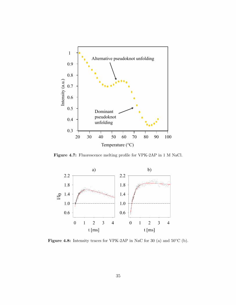
Melting profiles showing equilibrium intensity measurements for VPK-2AP and F-VPK

at different temperatures were taken by Velmurugu et al. [46]. Figure 4.7 shows the melting

profile for VPK-2AP in 1 M NaCl. The transitions at 51 and 77 ◦C are attributed to the

melting of the pseudoknot stems. In our experiments we observe the folding process from

extended to native conformation. Therefore we should read the melting plots from right to

left and stop at the temperature at which the experiment was conducted.

Read in such a way, for 30 ◦C the intensity should go up significantly and decrease slightly

at the end. For 40 and 50 ◦C the final decrease should be smaller and almost disappear. This

is exactly what our intensity data for VPK-2AP in NaC (with 1 M NaCl) looks like (figure

4.8). We identify the fast increase in intensity as the formation of stem 2 of pseudoknot

VPK upon an already formed stem 1, while the slower decay is due to the alternative folding

pathway in which stem 1 forms after stem 2. In agreement with the equilibrium data, the

alternative folding pathway vanishes for higher temperatures, since stem 2 melts at around

50 ◦C. A schematic drawing of the two pathways can be seen in figure 5.1.

34

Inte

nsity

(a.u

.)

Temperature (°C)

1 0.9 0.8 0.7 0.6 0.5 0.4 0.3 20 30 40 50 60 70 80 90 100

Alternative pseudoknot unfolding

Dominant pseudoknot unfolding

Figure 4.7: Fluorescence melting profile for VPK-2AP in 1 M NaCl.

Figure 4.8: Intensity traces for VPK-2AP in NaC for 30 (a) and 50◦C (b).

35

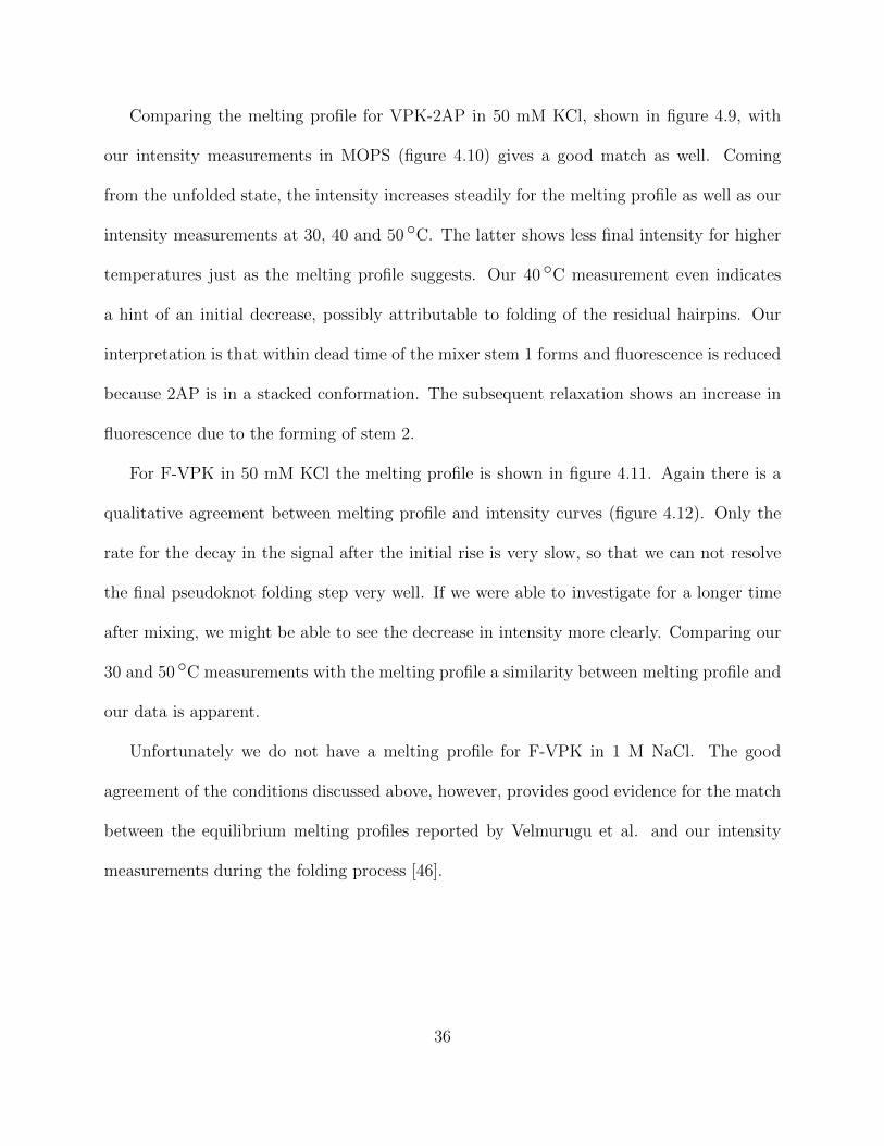
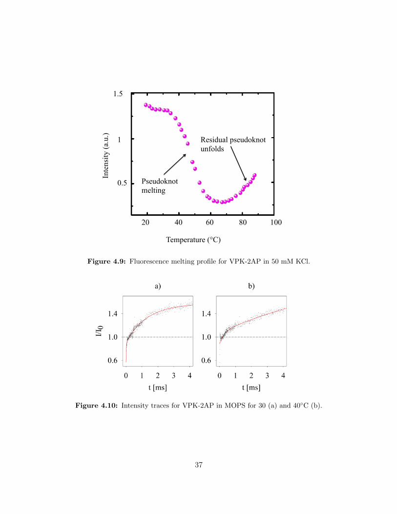
Comparing the melting profile for VPK-2AP in 50 mM KCl, shown in figure 4.9, with

our intensity measurements in MOPS (figure 4.10) gives a good match as well. Coming

from the unfolded state, the intensity increases steadily for the melting profile as well as our

intensity measurements at 30, 40 and 50 ◦C. The latter shows less final intensity for higher

temperatures just as the melting profile suggests. Our 40 ◦C measurement even indicates

a hint of an initial decrease, possibly attributable to folding of the residual hairpins. Our

interpretation is that within dead time of the mixer stem 1 forms and fluorescence is reduced

because 2AP is in a stacked conformation. The subsequent relaxation shows an increase in

fluorescence due to the forming of stem 2.

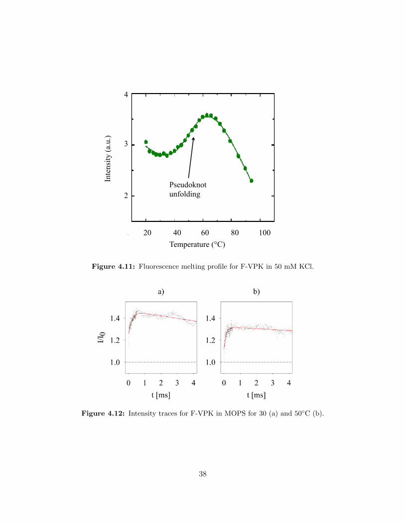
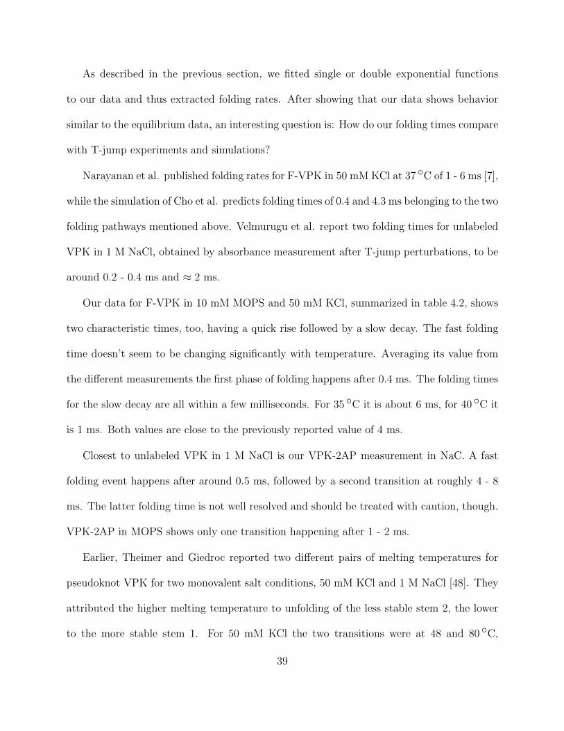
For F-VPK in 50 mM KCl the melting profile is shown in figure 4.11. Again there is a

qualitative agreement between melting profile and intensity curves (figure 4.12). Only the

rate for the decay in the signal after the initial rise is very slow, so that we can not resolve

the final pseudoknot folding step very well. If we were able to investigate for a longer time

after mixing, we might be able to see the decrease in intensity more clearly. Comparing our

30 and 50 ◦C measurements with the melting profile a similarity between melting profile and

our data is apparent.

Unfortunately we do not have a melting profile for F-VPK in 1 M NaCl. The good

agreement of the conditions discussed above, however, provides good evidence for the match

between the equilibrium melting profiles reported by Velmurugu et al. and our intensity

measurements during the folding process [46].

36

Inte

nsity

(a.u

.)

Temperature (°C)

1.5

20 40 60 80 100

Pseudoknot melting

1

0.5

Residual pseudoknot unfolds

Figure 4.9: Fluorescence melting profile for VPK-2AP in 50 mM KCl.

Figure 4.10: Intensity traces for VPK-2AP in MOPS for 30 (a) and 40◦C (b).

37

Inte

nsity

(a.u

.)

Temperature (°C)

4

20 40 60 80 100

Pseudoknot unfolding

3

2

Figure 4.11: Fluorescence melting profile for F-VPK in 50 mM KCl.

Figure 4.12: Intensity traces for F-VPK in MOPS for 30 (a) and 50◦C (b).

38

As described in the previous section, we fitted single or double exponential functions

to our data and thus extracted folding rates. After showing that our data shows behavior

similar to the equilibrium data, an interesting question is: How do our folding times compare

with T-jump experiments and simulations?

Narayanan et al. published folding rates for F-VPK in 50 mM KCl at 37 ◦C of 1 - 6 ms [7],

while the simulation of Cho et al. predicts folding times of 0.4 and 4.3 ms belonging to the two

folding pathways mentioned above. Velmurugu et al. report two folding times for unlabeled

VPK in 1 M NaCl, obtained by absorbance measurement after T-jump perturbations, to be

around 0.2 - 0.4 ms and ≈ 2 ms.

Our data for F-VPK in 10 mM MOPS and 50 mM KCl, summarized in table 4.2, shows

two characteristic times, too, having a quick rise followed by a slow decay. The fast folding

time doesn’t seem to be changing significantly with temperature. Averaging its value from

the different measurements the first phase of folding happens after 0.4 ms. The folding times

for the slow decay are all within a few milliseconds. For 35 ◦C it is about 6 ms, for 40 ◦C it

is 1 ms. Both values are close to the previously reported value of 4 ms.

Closest to unlabeled VPK in 1 M NaCl is our VPK-2AP measurement in NaC. A fast

folding event happens after around 0.5 ms, followed by a second transition at roughly 4 - 8

ms. The latter folding time is not well resolved and should be treated with caution, though.

VPK-2AP in MOPS shows only one transition happening after 1 - 2 ms.

Earlier, Theimer and Giedroc reported two different pairs of melting temperatures for

pseudoknot VPK for two monovalent salt conditions, 50 mM KCl and 1 M NaCl [48]. They

attributed the higher melting temperature to unfolding of the less stable stem 2, the lower

to the more stable stem 1. For 50 mM KCl the two transitions were at 48 and 80 ◦C,

39

while for 1 M NaCl these temperatures were shifted to higher temperatures, 70 and 95 ◦C.

Monovalent salt in the environment therefore stabilizes the pseudoknot structure. This

conclusion was confirmed by Holmstrom et al. [49]. Investigating the relationship between

formation of tertiary structure (a tetraloop-receptor) and Na+ concentration, they found a

clear relationship between salt concentration and the folding and unfolding rate: the higher

the concentration the larger (smaller) the folding (unfolding) rate.

Although the size of the counterions seems to have a slight effect on the folding rates, a

comparison of our results for the two folding conditions agrees with the general finding that

the higher the monovalent salt concentration is, the shorter are the folding times. Having a

look at VPK-2AP in NaC and MOPS, respectively, the early folding process for the higher

concentration occurs after around 0.6 ms, while for the lower one it starts only after 1 - 2 ms.

Similarly for F-VPK at high salt concentration we cannot resolve the early folding process,

but we can deduce that it is completed within the first 200 µs. For the lower concentration

the folding time is roughly 0.4 ms.

40

Chapter 5

Summary and outlook

Our folding experiments of RNA pseudoknot VPK exhibit different behaviors for different

solvent and labels. Overall, equilibrium melting plots and our folding traces match quite

well. This seems surprising, since we did not expect to see this adiabatic behavior in our fast-

folding experiment. For VPK-2AP in high salt concentration (1 M NaCl) we interpret our

data as showing two different folding pathways (see figure 5.1), while in low salt concentration

we can see only one transition. There could be two explanations for the “missing” transition:

either one of the stems forms within dead time of our instrument, or it forms on a longer

timescale than we can observe. We think the former is more likely, since according to the

equilibrium melting profile, the formation of the first hairpin loop occurs at high temperature

with a decay in fluorescence signal. Suppose that this formation happens within mixing time,

then indeed we wouldn’t see a drop in intensity, if drop and subsequent recovery both take

place very fast. The characteristic folding times are approximately 1 - 2 ms for the low and

0.5 ms and 4 - 8 ms for the high salt concentration, respectively.

41

Stem 1

Stem 2

Figure 5.1: Schematics of the folding pathway for VPK-2AP in sodium cacodylate with 1 MNaCl. The position of the intrinsic fluorescence label 2-AP is indicated by the small sun. Thebase pairing regions of stems 1 and 2 are drawn in red. The upper pathway represents thedominant folding pathway, where stem 1 forms first followed by stem 2.

42

Stem 1

Stem 2

Figure 5.2: Schematics of VPK-F. The fluorescein label is at the 5’-end of the RNA, close tostem 1 of the pseudoknot. It seems unclear, why the forming of stem 2 should have an effecton the fluorescence signal.

For the fluorescein-labeled F-VPK in high salt concentration we observed an initial strong

increase in fluorescence within dead time of our mixer, followed by a steep decline on a time

scale of around 0.6 ms. The decline could possibly consist of two processes, but we cannot

tell for sure. For the lower salt concentration we detected two folding phases. This is

in agreement with the equilibrium melting profiles for F-VPK. However, Velmurugu et al.

interpreted the decrease in fluorescence for higher temperatures as a temperature dependent

response of the fluorescein label [46]. Our kinetic data seems to provide evidence for another

transition in the RNA. At this time, we are not sure of the nature of this transition. It

might be due to a parallel folding pathway just the same as for VPK-2AP. But we cannot

tell yet, why the forming of stem 2 should affect the fluorescence signal of the fluorescein

label attached at the far other end of the RNA strand (see figure 5.2).

2-AP is very sensitive for different environments and shows different fluorescence prop-

erties even for nearest neighbours [50]. Including 2-AP labels at different positions could be

a way to rule out different folding pathways. Additionally, in order to rule out a change in

43

signal due to the mixing of 2-AP in the folding buffer, measurements of 2-AP alone should

be done.

Vieregg et al. showed that the size of the counterions matters in terms folding rate [47].

It could prove insightful to conduct measurements at different concentrations of the same

salt. This would make direct comparisons of different salt conditions possible. Also, a more

detailed investigation of the influence the size of counterions has on the RNA folding process

could reveal interesting findings and be helpful for the analysis of further experiments in the

future.

44

BIBLIOGRAPHY

45

BIBLIOGRAPHY

[1] I. Tinoco Jr. and C. Bustamante, J. Mol. Biol. 293, 271 (1999).

[2] P. G. Higgs, Q. Rev. Biophys. 33, 199 (2000).

[3] W. Gilbert, Nature 319, 618 (1986).

[4] J. Carter and V. Saunders, Virology: Principles and Applications ; Wiley: Chichester,2007; page 32.

[5] H. Yang, M. Yang, Y. Ding, Y. Liu, Z. Lou, Z. Zhou, L. Sun, L. Mo, S.Ye, H. Pang, G.F. Gao, K. Anand, M. Bartlam, R. Hilgenfeld, and Z. Rao, PNAS 100, 1390 (2003).

[6] G. Neumann, T. Noda, and Y. Kawaoka, Nature 459, 931 (2009).

[7] R. Narayanan, Y. Velmurugu, S. G. Kuznetsov, and A. Ansari, J. Am. Chem. Soc. 133,18767 (2011).

[8] C. Branden and J. Tooze, Introduction to Protein Structure; Garland Publishing, Inc.:New York, 1999; Chapter 2 and 6.

[9] M. Sela, F. H. White, and C. B. Anfinsen, Science 125, 691 (1957).

[10] S. B. Prusiner, Science 278, 5336 (1997).

[11] L. M. Luheshi, D. C. Crowther, and C. M. Dobson, Curr. Opin. Chem. Biol. 12, 25(2008).

[12] D. E. Draper, Biophys. J. 95, 5489 (2008).

[13] J. R. Wyatt, J. D. Puglisi, and I. Tinoco Jr., BioEssays 11, 100 (1989).

[14] R. Zwanzig, PNAS 94, 148 (2005).

46

[15] A. D. Robertson and K. D. Murphy, Chem. Rev. 97, 1251 (1997).

[16] Martin Karplus, Nat. Chem. Biol. 7, 401 (2011).

[17] A. Szilagyi, J. Kardos, S. Osvath, L. Barna, and P. Zavodszky, Protein Folding. InHandbook of Neurochemistry and Molecular Neurobiology, A. Lajtha and N. Banik, Eds.;Springer: New York, 2007; Vol. 7, Chapter 10, pp. 303-344.

[18] J. N. Onuchic, Z. Luthey-Schulten, and P. G. Wolynes, Annu. Rev. Phys. Chem. 48,545 (1997).

[19] K. A. Beauchamp, R. McGibbon, Y. Lin, and V. S. Pande, PNAS10.1073/pnas.1201810109 (published ahead of print July 9, 2012).

[20] A. B. Fulton and W. B. Isaacs, BioEssays 13, 157 (1991).

[21] C. Levinthal, How to fold Graciously. In Mossbauer Spectroscopy in Biological Systems:Proceedings of a meeting held at Allerton House, Monticello, Illinois, J. T. P. DeBrunnerand E. Munck, Eds., University of Illinois Press: Champaign, 1969; pp. 22-24.

[22] V. Pande and Stanford University (2012), The Science behind Folding@home. Retrievedfrom http://folding.stanford.edu/English/Science.

[23] K. Lindorff-Larsen, S. Piana, R. O. Dror, and D. E. Shaw, Science 334, 517 (2011).

[24] D. E. Shaw, M. D. Deneroff, R. O. Dror, J. S. Kuskin, R. H. Larson, J. K. Salmon,C. Young, B. Batson, K. J. Bowers, J. C. Chao, M. P. Eastwood, J. Gagliardo, J. P.Grossman, C. R. Ho, D. J. Ierardi, I. Kolossvry, J. L. Klepeis, T. Layman, C. McLeavey,M. A. Moraes, R. Mueller, E. C. Priest, Y. Shan, J. Spengler, M. Theobald, B. Towles,and S. C. Wang, Comm. of the ACM 51, 91 (2008).

[25] V. Pande and Stanford University (2012), Folding@home. Retrieved fromhttp://folding.stanford.edu/English/HomePage.

[26] H. A. Scheraga, M. Khalili, and A. Liwo, Annu. Rev. Phys. Chem. 58, 57 (2007).

[27] J. Kubelka, J. Hofrichter, and W. A. Eaton, Curr. Opin. Struct. Biol. 14, 76 (2004).

[28] T. R. Sosnick, Protein Sci. 17, 1308 (2008).

47

[29] W. A. Eaton, V. Munoz, S. J. Hagen, G. S. Jas, L. J. Lapidus, E. R. Henry, and J.Hofrichter, Annu. Rev. Biophys. Biomol. Struct. 29, 327 (2000).

[30] R. H. Webb, Rep. Prog. Phys. 59, 427 (1996).

[31] M. W. Davidson (2012), Basic Concepts and Formulas in Microscopy. Retrieved fromhttp://www.microscopyu.com/articles/formulas/formulasresolution.html.

[32] K. R. Spring, T. J. Fellers, and M. W. Davidson (2009),Resolution and Contrast in Confocal Microscopy. Retrieved fromhttp://www.olympusconfocal.com/theory/resolutionintro.html.

[33] J. B. Knight, A. Vishwanath, J. P. Brody, and R. H. Austin, Phys. Rev. Lett. 80, 3863(1998).

[34] L. Capretto, W. Cheng, M. Hill, and X. Zhang, Top. Curr. Chem. 304, 27 (2011).

[35] N.-T. Nguyen and S. T. Wereley, Fundamentals and Application of Microfluidics ; ArtechHouse, Inc.: Norwood, 2002, p. 39.

[36] L. J. Lapidus, S. Yao, K. S. McGarrity, D. E. Hertzog, and E. Tubman, Biophys. J. 93,218 (2007).

[37] D. E. Hertzog, X. Michalet, M. Jager, X. Kong, J. G. Santiago, S. Weiss, and O. Bakajin,Anal. Chem. 76, 7169 (2004).

[38] J. Kubelka, Photochem. Photobiol. Sci. 8, 499 (2009).

[39] S. Biyun, S. S. Cho, and D. Thirumalai, J. Am. Chem. Soc. 133, 20634 (2011).

[40] R. Narayanan, L. Zhu, Y. Velmurugu, S. V. Kuznetsov, L. Lapidus, and A. Ansari(2012) Exploring the energy landscape of nucleic acid hairpins using laser temperature-jump and microfluidic mixing. Manuscript submitted for publication.

[41] L. X. Shen and I. Tinoco, Jr, J. Mol. Biol. 247, 963 (1995).

[42] I. Brierley, S. Pennell, and R. G. C. Gilbert, Nat. Rev. Microbiol. 5, 598 (2007).

48

[43] J. M. Jean and K. B. Hall, PNAS 98, 37 (2000).

[44] U. D. Priyakumar, C. Hyeon, D. Thirumalai, and A. D. MacKerell, Jr, J. Am. Chem.Soc. 131, 17559 (2009).

[45] S. S. Cho, D. L. Pincus, and D. Thirumalai, PNAS 106, 17349 (2009).

[46] Y. Velmurugu, R. Narayanan, J. Roca, J. Liu, S. V. Kuznetsov, and A. Ansari, Laser T-jump studies of RNA pseudoknots reveal parallel folding/unfolding pathways. Poster sessionpresented at: Gordon Research Conferences 2012. Biopolymers - In Vitro, In Silico, andin the Cell. June 3-8, 2012. Newport, RI.

[47] J. Viergg, W. Cheng, C. Bustamante, I. Tinoco, Jr., J. Am. Chem. Soc. 48, 14966(2007).

[48] C. A. Theimer and D. P. Giedroc, RNA 6, 409 (2000).

[49] E. D. Holmstrom, J. L. Fiore, and D. J. Nesbitt, Biochem. 51, 3732 (2012).

[50] K. B. Hall and F. J. Williams, RNA 10, 34 (2000).

49