Introduction to Regression Techniques By Allan T. Mense, Ph.D., PE, CRE Principal Engineering Fellow, RMS

Table of Contents Introduction Regression and Model Building Simple Linear Regression (SLR) Variation of estimated Parameters

Analysis of Variance (ANOVA) Multivariate Linear Regression (MLR) Principal Components Binary Logistics Regression (BLR) Appendices GOS

Introduction. The purpose of this note is to try and lay out some of the techniques that are used to take data and deduce a response (y) or responses in terms of input variables (x values). This is a collection of topics and is meant to be a refresher not a complete text on the subject for which there are many. See the references section. These techniques fall into the broad category of regression analysis and that regression analysis divides up into linear regression and nonlinear regression. This first note will deal with linear regression and a follow-on note will look at nonlinear regression.

Regression analysis is used when you want to predict a continuous dependent variable or response from a number of independent or input variables. If the dependent variable is dichotomous, then logistic regression should be used.

The independent variables used in regression can be either continuous or dichotomous (i.e. take on a value of 0 or 1). Categorical independent variables with more than two values can also be used in regression analyses, but they first must be converted into variables that have only two levels. This is called dummy coding or indicator variables. Usually, regression analysis is used with naturally-occurring variables, as opposed to experimentally manipulated variables, although you can use regression with experimentally manipulated variables. One point to keep in mind with regression analysis is that causal relationships among the variables cannot be determined.

The areas I want to explore are 1) simple linear regression (SLR) on one variable including polynomial regression e.g. εββ ++= xy 10 , and 2) multiple linear regression

(MLR) or multivariate regression e.g. εβ += XY that uses vectors and matrices to represent the equations of interest. Included in my discussions are the techniques for

determining the coefficients ( β etc.) that multiply the variates (e.g. least squares, weighted least squares, maximum likelihood estimators, etc.). Under multivariate regression one has a number of techniques for determining equations for the response in terms of the variates: 1) design of experiments (DOE), and 2) point estimation method (PEM), are useful if data does not already exist, 3) stepwise regression either forward or backward, 4) principal components analysis (PCA), 5) canonical correlation analysis (CCA), 6) Generalized Orthogonal Solutions (GOS), and 7) partial least squares (PLS) analysis are useful when data already exists and further experiments are either not possible or not affordable. Regression analysis is much more complicated that simply “fitting a curve to data.” Anybody with more courage than brains can put data into excel or some other program and generate a curve fit, but how good is the fit? Are all the input variables important? Are there interactions between the input variables that affect the response(s)? How does one know if some terms are significant and others are not? Does the data support the postulated model for the behavior? These questions are not answered by simply “curve fitting.” I will try to address these issues. The important topic of validation of regression models will be save for a third note.

Regression and Model Building. Regression analysis is a statistical technique for investigating the relationship among variables. This is all there is to it. Everything else is how to do it, what the errors are in doing it, and how you make sense of it. In addition, there are a few cautionary tales that will be included at the right places! Of course there are volumes of papers and books covering this subject so someone thinks there is a lot more to regression than simply fitting a curve to data. This is very true!

Note: While the terminology is such that we say that X "predicts" Y, we cannot say that X "causes" Y even though one many times says the ‘X” variables are causal variables we really mean that “X” shows a trending relationship with the response “Y.” We cannot even say Y is correlated with X if the X-values are fixed levels of some variable i.e. if X is not a random variable. Correlation (and covariance) only applies between random variables and then it is a measure of only a linear relationship. This may seem too subtle to bring up right now but my experience is that it is better said early in the study of this subject and thus keep our definitions straight.

Let’s start with the easy stuff first by way of an example. Example Data: A rocket motor is manufactured by bonding an igniter propellant and a sustainer propellant together inside a metal housing (Montgomery, et al.). The shear strength of the bond is an important quality characteristic that can affect the reliability and availability of the rocket. It is suspected (engineering judgment) that the shear

strength is related to the age in weeks of the batch of sustainer propellant used in the bonding. Here are 20 observations on the shear strength vs. age of sustainer batch production.

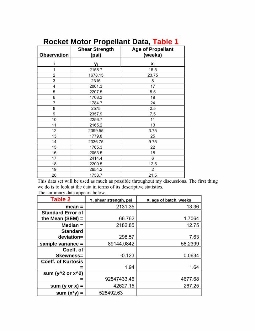
Rocket Motor Propellant Data, Table 1 Observation

Shear Strength (psi)

Age of Propellant (weeks)

i yi xi 1 2158.7 15.5 2 1678.15 23.75 3 2316 8 4 2061.3 17 5 2207.5 5.5 6 1708.3 19 7 1784.7 24 8 2575 2.5 9 2357.9 7.5 10 2256.7 11 11 2165.2 13 12 2399.55 3.75 13 1779.8 25 14 2336.75 9.75 15 1765.3 22 16 2053.5 18 17 2414.4 6 18 2200.5 12.5 19 2654.2 2 20 1753.7 21.5

This data set will be used as much as possible throughout my discussions. The first thing we do is to look at the data in terms of its descriptive statistics. The summary data appears below.

Table 2 Y, shear strength, psi X, age of batch, weeks mean = 2131.35 13.36

Standard Error of the Mean (SEM) = 66.762 1.7064

Median = 2182.85 12.75 Standard

deviation= 298.57 7.63 sample variance = 89144.0842 58.2399

Coeff. of Skewness= -0.123 0.0634

Coeff. of Kurtosis = 1.94 1.64

sum (y^2 or x^2) = 92547433.46 4677.68

sum (y or x) = 42627.15 267.25 sum (x*y) = 528492.63

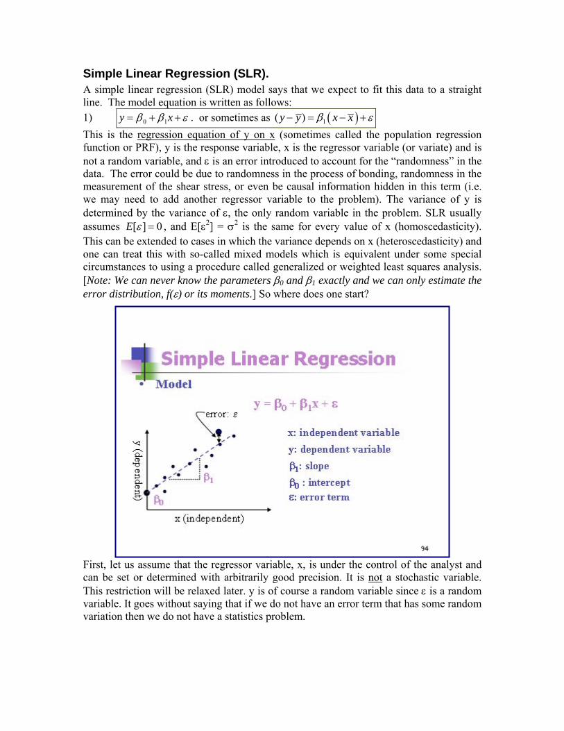
Simple Linear Regression (SLR). A simple linear regression (SLR) model says that we expect to fit this data to a straight line. The model equation is written as follows: 1) εββ ++= xy 10 . or sometimes as ( )1( )y y x x− β ε= − + This is the regression equation of y on x (sometimes called the population regression function or PRF), y is the response variable, x is the regressor variable (or variate) and is not a random variable, and ε is an error introduced to account for the “randomness” in the data. The error could be due to randomness in the process of bonding, randomness in the measurement of the shear stress, or even be causal information hidden in this term (i.e. we may need to add another regressor variable to the problem). The variance of y is determined by the variance of ε, the only random variable in the problem. SLR usually assumes 0][ =εE , and E[ε2] = σ2 is the same for every value of x (homoscedasticity). This can be extended to cases in which the variance depends on x (heteroscedasticity) and one can treat this with so-called mixed models which is equivalent under some special circumstances to using a procedure called generalized or weighted least squares analysis. [Note: We can never know the parameters β0 and β1 exactly and we can only estimate the error distribution, f(ε) or its moments.] So where does one start?

First, let us assume that the regressor variable, x, is under the control of the analyst and can be set or determined with arbitrarily good precision. It is not a stochastic variable. This restriction will be relaxed later. y is of course a random variable since ε is a random variable. It goes without saying that if we do not have an error term that has some random variation then we do not have a statistics problem.

For any given value of x, y is distributed about a mean value, [ ]|E y x , and the distribution is the same as the distribution of ε, i.e. var(y)=var(ε). Since the expected value of ε is assumed to be zero, the expected value or mean of this distribution of y, given the regressor value x, is 2) [ ] xxyE 10| β += β . It is this equation we wish to model. The variance of y given x is given by the formula 3) [ ] ( ) 2

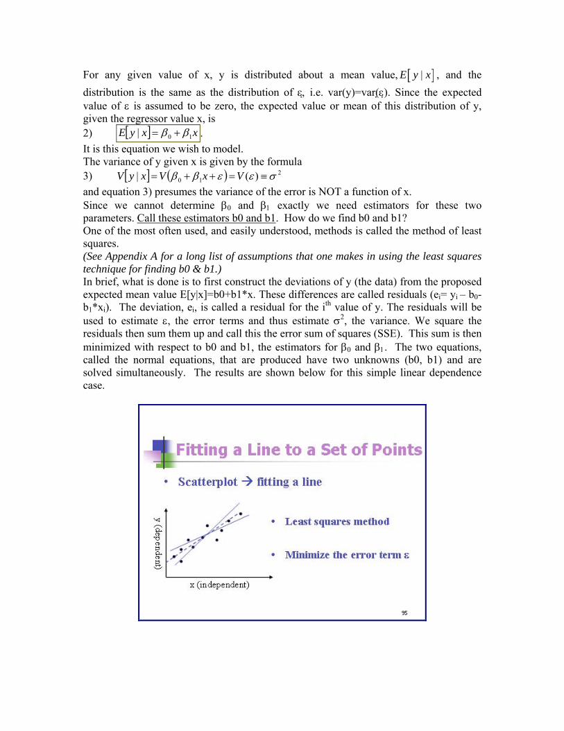
10 )(| σεεββ ≡=++= VxVxyVand equation 3) presumes the variance of the error is NOT a function of x. Since we cannot determine β0 and β1 exactly we need estimators for these two parameters. Call these estimators b0 and b1. How do we find b0 and b1? One of the most often used, and easily understood, methods is called the method of least squares. (See Appendix A for a long list of assumptions that one makes in using the least squares technique for finding b0 & b1.) In brief, what is done is to first construct the deviations of y (the data) from the proposed expected mean value E[y|x]=b0+b1*x. These differences are called residuals (ei= yi – b0-b1*xi). The deviation, ei, is called a residual for the ith value of y. The residuals will be used to estimate ε, the error terms and thus estimate σ2, the variance. We square the residuals then sum them up and call this the error sum of squares (SSE). This sum is then minimized with respect to b0 and b1, the estimators for β0 and β1. The two equations, called the normal equations, that are produced have two unknowns (b0, b1) and are solved simultaneously. The results are shown below for this simple linear dependence case.

4) ( ) ( )2

1 1 10 1 0 1

1 10

0 2 1

n

i n ni

i i in ni i

e

1

n

ii

y b b x b y b xb

=

= =

∂= = − − − ⇒ = −

∂

∑∑ ∑

=∑

This is well detailed in the literature (Ref 1, pg 13) and the result is 4a) 0 1 *b y b x= − where y , x are the averages of the measured values and

5) ( ) ( )2 1

1 10 1 2

11 2 1

1 1

0 2 1 1

n n

i i nni i

i i i n nii in

i i

e xx y b b x b

bx x

= =

=

= =

∂ −= = − − − ⇒ =

∂ ⎛ ⎞− ⎜ ⎟

⎝ ⎠

∑ ∑∑

∑ ∑1 1

n n

i i ii i

y x y= =∑ ∑

5a) ( )( ) ( )2

1 11 , ,

n nxy

xy j j xx jxx j j

Sb S y y x x S xS= =

= = − − =∑ ∑ x−

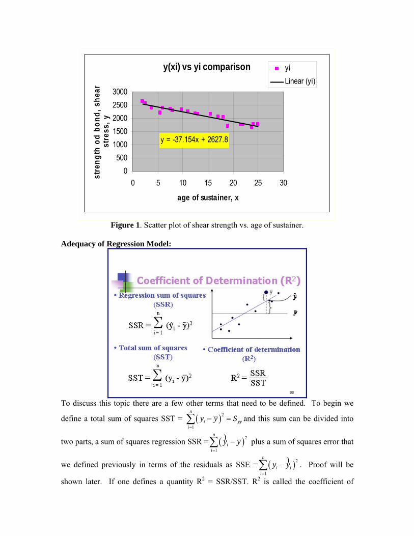
We now have an equation to estimate the mean value of y (shear stress in psi) in terms of the age, x (weeks) of the batch of the sustainer propellant used in the rocket motor. This equation gives the expected value of shear stress at a specified value of batch age and is simply 6) ˆ[ | ] 0 1*E y x y b b x≡ = + . This is the fitted regression line or sample regression function (SRF). It measures the location of the expected mean value of a number of measurements of y given x. This all seems easy! Just wait. We can make the easiest of methods very complicated. A note to the wise. Do not use equation, 6), to predict vales for E[y|x] outside the limits of the x and y values you use to determine the coefficients b0 and b1. This is NOT an extrapolation formula. Let’s do the math for the example shown in Table 1.

Variable Value Sxy = -41112.65 Sxx = 1106.56 Syy = 1693737.60 b1 = -37.15 b0 = 2627.82

If we plot the data values yi vs. xi (called a scatter plot) and compare them to the values obtained from equation 6) above we can see how well this works on this particular problem. Looking at Figure 1 below, the linear fit appears to be quite good and one could use a number of measures to show this quantitatively.

y(xi) vs yi comparison

y = -37.154x + 2627.8

0500

10001500200025003000

0 5 10 15 20 25 30

age of sustainer, x

stre

ngth

od

bond

, she

ar

stre

ss, y

yiLinear (yi)

Figure 1. Scatter plot of shear strength vs. age of sustainer.

Adequacy of Regression Model:

To discuss this topic there are a few other terms that need to be defined. To begin we

define a total sum of squares SST = ( )2

1

n

ii

yyy y S=

− =∑ and this sum can be divided into

two parts, a sum of squares regression SSR = ( 2

1

n

ii

)y y=

−∑ ) plus a sum of squares error that

we defined previously in terms of the residuals as SSE = ( 2

1

n

i ii

)y y=

−∑ ) . Proof will be

shown later. If one defines a quantity R2 = SSR/SST. R2 is called the coefficient of

determination. It is the proportion of the variation of y that is explained by the regressor variable x. For the above problem R2 = 0.9018 which is fairly good. Values of R2 close to 1 imply that most of the variability of y is explained by x. Problem is done, yes? NOT YET.

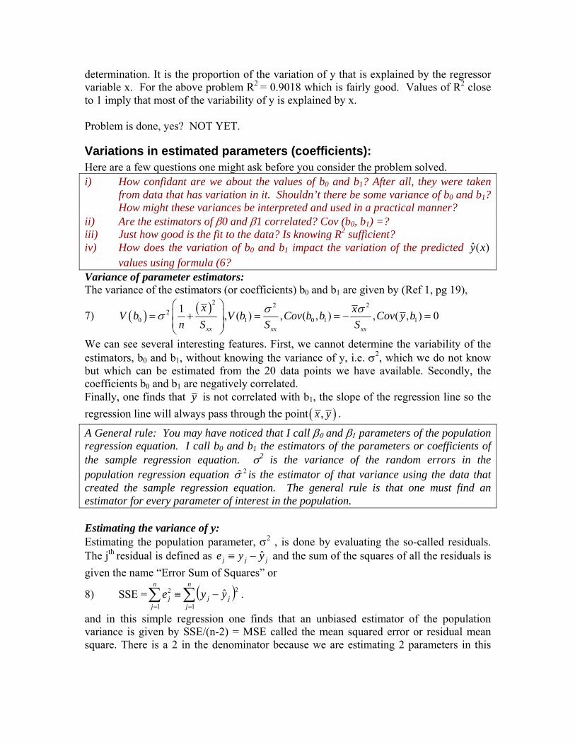
Variations in estimated parameters (coefficients): Here are a few questions one might ask before you consider the problem solved. i) How confidant are we about the values of b0 and b1? After all, they were taken

from data that has variation in it. Shouldn’t there be some variance of b0 and b1? How might these variances be interpreted and used in a practical manner?

ii) Are the estimators of β0 and β1 correlated? Cov (b0, b1) =? iii) Just how good is the fit to the data? Is knowing R2 sufficient? iv) How does the variation of b0 and b1 impact the variation of the predicted )(ˆ xy

values using formula (6? Variance of parameter estimators: The variance of the estimators (or coefficients) b0 and b1 are given by (Ref 1, pg 19),

7) ( ) ( )2 2 22

0 1 0 11 , ( ) , ( , ) , ( , ) 0

xx xx xx

x xV b V b Cov b b Cov y bn S S S

σ σσ⎛ ⎞⎜ ⎟= + = = − =⎜ ⎟⎝ ⎠

1

We can see several interesting features. First, we cannot determine the variability of the estimators, b0 and b1, without knowing the variance of y, i.e. σ2, which we do not know but which can be estimated from the 20 data points we have available. Secondly, the coefficients b0 and b1 are negatively correlated. Finally, one finds that y is not correlated with b1, the slope of the regression line so the regression line will always pass through the point ( ),x y .

A General rule: You may have noticed that I call β0 and β1 parameters of the population regression equation. I call b0 and b1 the estimators of the parameters or coefficients of the sample regression equation. σ2 is the variance of the random errors in the population regression equation is the estimator of that variance using the data that 2σcreated the sample regression equation. The general rule is that one must find an estimator for every parameter of interest in the population. Estimating the variance of y: Estimating the population parameter, σ2 , is done by evaluating the so-called residuals. The jth residual is defined as jjj yye ˆ−≡ and the sum of the squares of all the residuals is given the name “Error Sum of Squares” or

8) SSE = . ( )∑∑==

−≡n

jjj

n

jj yye

1

2

1

2 ˆ

and in this simple regression one finds that an unbiased estimator of the population variance is given by SSE/(n-2) = MSE called the mean squared error or residual mean square. There is a 2 in the denominator because we are estimating 2 parameters in this

example (β0 and β1). Again it can be shown (ref 1, pg 16) that the best estimator of the variance of y, E[ ] = σ2, is given by 2σ

9) ( )∑=

−−

=−

=n

jjj yy

nnSSE

1

22 ˆ2

1)2(

σ .

Since is an estimator of the variance we can prescribe a confidence interval for if we can say something about how the errors are distributed, i.e. if we presume that errors are normally distributed, then we can use the chi-squared distribution and bound σ2 by the confidence interval shown below which assumes a 95% confidence level.

2σ 2σ

10) 2220,2/975.0

22

220,2/05.0

)2()2(

−−

−≤≤

−χ

σχ

MSEnMSEn

(Note: For the above confidence interval to be correct the random errors should be normally distributed with variance =σ2 = constant for all values of x.). Digression: Note that we can calculate a number of point estimators (b0, b1, ) but 2σthey do us little good unless we know something about how the random variation is distributed. When we calculated estimators that make use of the sum of many small errors then we can invoke the central limit theorem (and the theorem of large numbers) to let us use the normal distribution as a good guess. This assumption allowed us to use χ2 distribution to find a confidence interval for the population variance. This assumption is even useful for small samples (e.g. n=20) and can be tested as will be shown later in this note. In this day and age of computers, we can use other distributions or even nonparametric statistics. Confidence interval for β1: This is also a confidence interval problem. In the analysis we just performed we wished to know β1 and to do this we calculated the estimator b1. Reference 1 again gives the following formula for the 95% confidence interval for β1.

11) 1 .05/ 2,20 2 1 .05/ 2,20 2ˆ

,20 20

b t b tσ− −

⎛ ⎞− +⎜ ⎟

⎝ ⎠

σ= (-43.2,-31.1)

for the example shown in Table 1. Again, one assumes the errors are normally distributed and the sample size is small. What does this mean? For this specific case, and stating it loosely, one says the above interval is constructed in such a manner that we are 95% confident that the actual β1 value is between -43.2 and -31.1 based upon the n=20 sample data set in Table 1. Another way of saying the same thing is that even though the estimated value E[b1] = -37.15, the real value of β1 should fall between -43.2 and -31.1 with 95% confidence. Thus it could be as low as -43.2 or as high as -31.3. We have only narrowed down our estimate of β1 to b1*(1 +/- 16.3%). At least if we want to be 95% confident of our results. If we want a tighter interval about b1 then we need to have a larger sample size, n or be willing to live with a lower level of confidence. If n=180 instead of 20 we would find the actual interval would be smaller by about a factor of 3 on each side of b1.

Confidence interval for β0: The confidence interval for β0 for this specific example (ref 1, pg 25) is given by the following for confidence level = 95%:

12) 2 2

0 .05/ 2,20 2 0 .05/ 2,20 21 1,

xx xx

x xb t MSE b t MSEn S n S− −

⎛ ⎞⎛ ⎞ ⎛ ⎞⎜ ⎟− + +⎜ ⎟ ⎜ ⎟⎜ ⎟⎝ ⎠ ⎝ ⎠⎝ ⎠+

0

Confidence interval for the mean value of y at a given x value, E[y|X=x0]. The formula is 0 0 0 1ˆ( ) ( | ) *y x E y x b b x= = + and the confidence interval for E[y|x0] is given by the following formula, again using n=20 from the example we are using with n=20 data points and setting the confidence level to 95%: 13)

( ) ( )2 20 0

.05/ 2,20 2 .05/ 2,20 21 1ˆ ˆ( ) , ( )20 20o o

xx xx

x x x xy x t MSE y x t MSE

S S− −

⎛ ⎞⎛ ⎞ ⎛ ⎞− −⎜ ⎟− + + +⎜ ⎟ ⎜ ⎟⎜ ⎟ ⎜ ⎟⎜ ⎟⎝ ⎠ ⎝ ⎠⎝ ⎠

Prediction interval for y itself at a given value of x, y(xi). Finally if we wish to know the prediction interval for a new set of m observations there is the formula

14) ⎟⎟

⎠

⎞

⎜⎜

⎝

⎛⎥⎦

⎤⎢⎣

⎡ −++Δ+⎥

⎦

⎤⎢⎣

⎡ −++Δ−

xx

ii

xx

ii S

xxn

MSExyS

xxn

MSExy22 )(11)(ˆ,)(11)(ˆ

where 1.mfor 2,2 ==Δ −ntα Note the interval for the prediction about y(xi) is greater than the confidence interval for the mean value. [Why?] There are also methods for the simultaneous bounding of b0 and b1 instead of the “rectangular bounds” imposed by the equations 11) and 12). For m>1 there are other methods for determining the correct value of Δ. (See Ref 1, pg 32 for Bonferroni method). All this is pretty well known and establishes a base from which we can explore other regression techniques. Lack of fit (LOF): There is a formal statistical test for “Lack of Fit” of a regression equation. The procedure assumes the residuals are normally distributed, independent of one another and that the variance is a constant. Under these conditions and assuming only the linearity of the fit is in doubt one proceeds as follows. We need to have data with at least one repeat observation one or more levels of x. (See appendix for discussion of replication vs. repetition). Begin by partitioning the sum of squares error into two parts. SSE=SSPE + SSLOF. The parts are found by using the formulation ( ) ( ) ( )ij i ij i i iy y y y y y− = − + −) ) and squaring both sides followed by summing over the m-levels of x and the ni values measured at each level. I.e.

15) SSE= ( ) ( ) ( )2 2 2

1 1 1 1 1

i in nm m m

ij i ij i i i ii j i j i

y y y y n y= = = = =

− = − + −∑∑ ∑∑ ∑) )y

which produces the obvious definitions for the “pure error”

16) ( )2

1 1

inm

PE ij ii j

SS y y= =

≡ −∑∑

and for the “lack of fit” term,

17) ( )2

1

m

LOF i i ii

SS n y y=

≡ −∑ ) .

The justification of this partitioning is that the double sum in the SSPE term represents the corrected sum of squares of the repeat observations at each level of x and then pooling those errors over the m levels of x. If the assumption of constant variance is true then this double sum is a model independent measure of pure error since only the variability of y at each x level is used to compute SSPE. Since there are ni-1 degrees of freedom for

pure error at each of the m levels them ( )1

1m

ii

n n=

m− = −∑ degrees of freedom total.

Similarly for the SSLOF term we see that it is a weighted sum of squared deviations between the response iy at each level of x and the fitted values iy) . If the fitted values are close to each level mean value then one has a good fit. To the extent that SSLOF is large on has a lack of fit. There are m-2 degrees of freedom associated with SSLOF since one needs 2 degrees to obtain the b0 and b1 coefficients in the model. The test statistic for

lack of fit is 0( 2)

( )

LOF

LOF

PE PE

SSMSmF SS MS

n m

−≡ =

−

and since the expected value of MSPE = σ2 and

the expected value of MSLOF can be shown to be (ref 1, pg 87)

( )20 1

2 1[ ]

[ ]2

m

i i ii

LOF

n E y b b xE MS

mσ =

− −= +

−

∑ then, if the regression function produces a

good linear fit to the data E[MSLOF] =σ2 this implies F0 ~ 1.0. Under this situation F0 is distributed as an F distribution, more specifically as Fm-2,n-m . Therefore if F0 >> Fα,m-2,n-m one has reason to reject the hypothesis that a linear fit is a good fit with some confidence level 1-α.. If rejected then the fit must be nonlinear either in the variables or in the functional form of the fitting equation. We will address higher order fitting later in this note and will discuss nonlinear regression in a later note. Now let’s look at the analysis of variance which is a standard step in regression analysis.

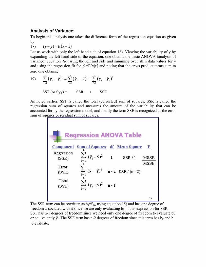
Analysis of Variance: To begin this analysis one takes the difference form of the regression equation as given by 18) ( )xxbyy −=− 1)ˆ( Let us work with only the left hand side of equation 18). Viewing the variability of y by expanding the left hand side of the equation, one obtains the basic ANOVA (analysis of variance) equation. Squaring the left and side and summing over all n data values for y and using the regression fit for y =E[y|x] and noting that the cross product terms sum to zero one obtains;

19) ( ) ( ) (∑∑∑===

−+−=−n

iii

n

ii

n

ii yyyyyy

1

2

1

2

1

2 ˆˆ )

SST (or Syy) = SSR + SSE As noted earlier, SST is called the total (corrected) sum of squares; SSR is called the regression sum of squares and measures the amount of the variability that can be accounted for by the regression model, and finally the term SSE is recognized as the error sum of squares or residual sum of squares.

The SSR term can be rewritten as b1*Sxy using equation 15) and has one degree of freedom associated with it since we are only evaluating b1 in this expression for SSR. SST has n-1 degrees of freedom since we need only one degree of freedom to evaluate b0 or equivalently y . The SSE term has n-2 degrees of freedom since this term has b0 and b1 to evaluate.

To test the significance of the regression model one again makes use of the F-test where the F statistic is given by

20) MSEMSR

nSSE

SSRF =

−=

)2(

10

Noting that the expected values of these terms are given by 21) xxSMSRE 2

12][ βσ +=

and 22) 2][ σ=MSEE

the F statistic represents in the limit 2

21

0 1 σβ xxSF +≈

Thus F>>1 implies the regression analysis is significant i.e. β1 is not zero so there is a significant linear dependency that is represented by the regression. How big must F0 become to be considered significant? Up to this point, we have calculated variances and standard deviations from the statistical data. One cannot however interpret these measures of variability without a model of how the randomness of the variables is distributed. For example, what is the probability that β1 might be between 11 2 bb σ± ) ? The answer is you don’t know unless you know how β1 is distributed? If it is distributed normally then ~95.4% of the range of β1 lies within 2 standard deviations of b1. If it is distributed in some other way then this is not true. So it is incorrect to think that regression analysis is simply curve fitting. How one interprets the exactness of the “fit” is dependent on the statistical distribution of the error term in the population regression equation and the assumptions about how the independent variables are or are not correlated Summary: From data one has fitted a straight line, the best straight line possible in the sense that the intercept (b0) and the slope (b1) have the smallest variance given the n=20 data points at hand. We have given formulas that calculate the variance of the estimators b0, b1 and found the intervals bounding the predicted expected value of y at a given x=x0, and the prediction of the actual value of y at x=x0.

Multivariate Linear Regression (MLR). Taking the above univariate analysis and moving it into multiple dimensions requires the use of matrix algebra. This is easily done but takes some getting used to. The easiest equational model is shown below 23) 0 1 1 2 2 , 1, 2, ,i i i k iky x x x i nβ β β β= + + + + =L L and xik is the ith measured value of the kth regressor variable. In matrix notation

24)

1 11 1 0

2 21 2 1

1

11

1

k

k

n n nk n

y x xy x x

y x x

1

2

n

β εβ ε

β ε

⎡ ⎤ ⎡ ⎤ ⎡ ⎤ ⎡ ⎤⎢ ⎥ ⎢ ⎥ ⎢ ⎥ ⎢ ⎥⎢ ⎥ ⎢ ⎥ ⎢ ⎥ ⎢ ⎥= +⎢ ⎥ ⎢ ⎥ ⎢ ⎥ ⎢ ⎥⎢ ⎥ ⎢ ⎥ ⎢ ⎥ ⎢ ⎥⎢ ⎥ ⎢ ⎥ ⎢ ⎥ ⎢ ⎥⎣ ⎦ ⎣ ⎦ ⎣ ⎦ ⎣ ⎦

LL

M M M L M M ML

or

25) y X β ε= + . I will drop the underlining notation when the vector/matrix nature of the problem is well understood. Everything noted from the univariate analysis is true here with the exception that one may have covariance between y variables. The solution vector for the estimator of β is called b and is given by (ref 1, pg 122), 26) ( ) 1' 'y Xb X X X X y Hy

−= = ≡) therefore

27) ( ) 1'b X X X−

= ' y

1

2

3

n

. The actual terms are shown in appendix B. An example may be useful at this point. One is interested in the pull strength of a wirebond to a printed circuit board. The variables that appear to be relevant are the length of the wire being bonded and the height of the die of the chip. The following experimental data on pull strength (Y) vs. wire length (X1) and die height (X2) are shown below. We wish to find a formula for Y in terms of X1 and X2. The population regression model: E[Y|x1,x2] = β0 + β1*x1 + β2* x2 + ε and the sample regression function is given by,

E[Y|x1,x2] = b0 + b1*x1 + b2* x2 The vector of coefficients is found from the above formulas to be b = (b0,b1,b2) = (X’X)-1X’Y

1 0 1 11 2 2

2 0 1 12 2 2

3 0 1 13 2 2

0 1 1 2 2n n

y x xy x xy x x

y x x

β β ββ β ββ β β

β β β

= + += + += + +

= + +M

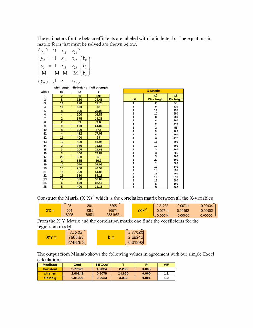
The estimators for the beta coefficients are labeled with Latin letter b. The equations in matrix form that must be solved are shown below.

1 11 21

2 12 22

3 13 23

2

1 2

111

1n n n

y x x

0

1

y x x by x x b

by x x

⎛ ⎞ ⎛ ⎞⎜ ⎟ ⎜ ⎟⎛ ⎞⎜ ⎟ ⎜ ⎟⎜ ⎟⎜ ⎟ ⎜ ⎟= ⎜ ⎟⎜ ⎟ ⎜ ⎟⎜ ⎟

⎝ ⎠⎜ ⎟ ⎜ ⎟⎜ ⎟ ⎜ ⎟⎝ ⎠ ⎝ ⎠

M M M M

25 204 8295X'X = 204 2382 76574

8295 76574 3531953

0.21232 -0.00711 -0.00034(X'X)-1 -0.00711 0.00162 -0.00002

-0.00034 -0.00002 0.00000

Construct the Matrix (X’X)-1 which is the correlation matrix between all the X-variables From the X’Y Matrix and the correlation matrix one finds the coefficients for the regression model

The output from Minitab shows the following values in agreement with our simple Excel calculation.

Predictor Coef SE Coef T P VIFConstant 2.77628 1.2324 2.253 0.035wire len 2.69242 0.1078 24.985 0.000 1.2die heig 0.01292 0.0033 3.952 0.001 1.2

wire length die height Pull strengthObs # x1 x2 Y

1 2 50 9.952 8 110 24.453 11 120 31.754 10 550 355 8 295 25.026 4 200 16.867 2 375 14.388 2 53 9.69 9 100 24.3510 8 300 27.511 4 412 17.0812 11 400 3713 12 500 41.9514 2 360 11.6615 3 205 21.6516 3 400 17.8917 20 600 6918 1 585 10.319 10 540 34.9320 15 250 46.5921 15 290 44.8822 16 510 54.1223 17 590 56.6324 6 100 22.1325 5 400 21.15

X-Matrixx1 x2

unit Wire length Die height1 2 501 8 1101 11 1201 10 5501 8 2951 4 2001 2 3751 2 531 9 1001 8 3001 4 4121 11 4001 12 5001 2 3601 3 2051 3 4001 20 6001 1 5851 10 5401 15 2501 15 2901 16 5101 17 5901 6 1001 5 400

725.82X'Y = 7968.93

274826.3

2.77628b = 2.69242

0.01292

Principal Components Analysis (PCA) Principal components are linear combinations of random variables that have special properties in terms of variances. For example, the first principal component is the normalized linear combination with maximum variance. In effect, PCA transforms the original vector variable to the vector of principal components which amounts to a rotation of coordinate axes to a new coordinate system that has some useful inherent statistical properties. In addition, principal components vectors turn out to be characteristic vectors of the covariance matrix. This technique is useful when there are lots of data and one wants to reduce the number of vectors needed to represent the useful data. It is in essence a variable reduction technique. Correctly used PCA separates the meaningful few variables from the “trivial many.” Suppose random vector X has p components each of length n. The covariance matrix is given by Σ. e.g.

1

p

XX

X

⎛ ⎞⎜

= ⎜⎜ ⎟⎝ ⎠

M⎟⎟ [ ],E Xμ ≡ [( )( ) '] [ '] 'E X X E XXμ μ μμΣ ≡ − − = −

and recalling the matrix operations if Y DX f= + then [ ] [ ]E Y DE X f= + and the covariance of Y is given by 'Y D DΣ = Σ . Let β be a p-component column vector such that ββ’=1. The variance of β’X is given by,

( )2[ ' ] ' ' 'E X E XXβ β β β⎡ ⎤ β= = Σ⎣ ⎦

To determine the normalized linear combination ' Xβ with maximum variance, one must find a vector b satisfying β’β=1 which maximizes the variance. This accomplished by

maximizing ( ) 2' ' 1 i ij j ii j i

φ β β λ β β β σ β λ β⎛= Σ − − = − −⎜⎝ ⎠

∑∑ ∑ 1⎞⎟ where λ is a

Lagrange multiplier.

2 2φ β λββ

∂= Σ −

∂ = 0 leads to solving the following eigenvalue equation for λ. Then λ is

substituted back to obtain the eigenvectors β . ( ) 0Iλ βΣ − =

In order to have non-trivial solution for b, one requires 0IλΣ − = which is a polynomial

in λ of degree p.

Noting that pre-multiplying φβ

∂∂

by β ’ gives ' 'β β λβ β λΣ = = and shows that if β

satisfies the eigenvalue equation and the normalization condition, β ’ β =1, then the variance( β ’X)=λ. Thus for maximum variance we should use the largest eigenvalue, λ = λ1, and the corresponding eigenvector, β(1). So let b(1) be the normalized solution to ( ) (1)

1 0Iλ βΣ − = then U1=β(1)’X is a normalized linear combination with maximum variance. Now one needs to find the vector that has maximum variance and is uncorrelated with U1. Lack of correlation implies (1) (1) (1)

1 1[ ' ] [ ' ' ] ' ' 0E XU E XXβ β β β β λ β β= = Σ = = which in turn means that b’X is orthogonal to U1 in both the statistical sense (lack of correlation) and in the geometric sense (inner product of vectors β and β(1) equals zero). Now one needs to maximize φ2 where, ( ) (1)

2 1' ' 1 2 'φ β β λ β β ν β β≡ Σ − − − Σ and λ and ν1

are Lagrange multipliers. Again setting 2 0φβ

∂=

∂ one obtains –2ν1λ1=0 which implies

ν1=0 and β must again satisfy the eigenvalue equation. Let λ2 be the maximum eigenvalue that is solution to ( )2 0 and ' 1Iλ β β βΣ − = = . Call this solution β(2) and

U2=β(2)’X is the linear combination with maximum variance that is orthogonal to β(1). The process can continue until there are p principal components as there were p initial variables. Hopefully one does not need all p principal components and the problem can be usefully solved with many fewer components. Otherwise there is not much advantage to using principal components.

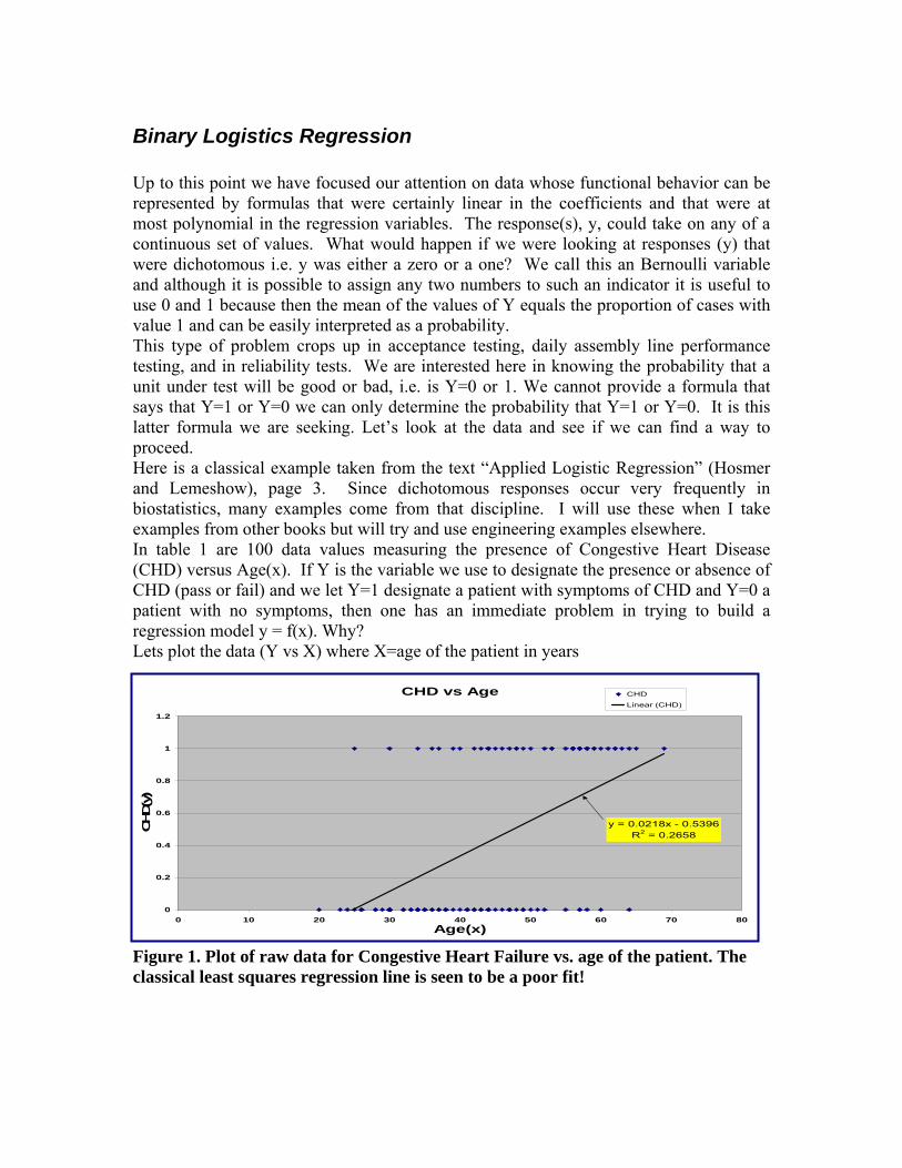
Binary Logistics Regression Up to this point we have focused our attention on data whose functional behavior can be represented by formulas that were certainly linear in the coefficients and that were at most polynomial in the regression variables. The response(s), y, could take on any of a continuous set of values. What would happen if we were looking at responses (y) that were dichotomous i.e. y was either a zero or a one? We call this an Bernoulli variable and although it is possible to assign any two numbers to such an indicator it is useful to use 0 and 1 because then the mean of the values of Y equals the proportion of cases with value 1 and can be easily interpreted as a probability. This type of problem crops up in acceptance testing, daily assembly line performance testing, and in reliability tests. We are interested here in knowing the probability that a unit under test will be good or bad, i.e. is Y=0 or 1. We cannot provide a formula that says that Y=1 or Y=0 we can only determine the probability that Y=1 or Y=0. It is this latter formula we are seeking. Let’s look at the data and see if we can find a way to proceed. Here is a classical example taken from the text “Applied Logistic Regression” (Hosmer and Lemeshow), page 3. Since dichotomous responses occur very frequently in biostatistics, many examples come from that discipline. I will use these when I take examples from other books but will try and use engineering examples elsewhere. In table 1 are 100 data values measuring the presence of Congestive Heart Disease (CHD) versus Age(x). If Y is the variable we use to designate the presence or absence of CHD (pass or fail) and we let Y=1 designate a patient with symptoms of CHD and Y=0 a patient with no symptoms, then one has an immediate problem in trying to build a regression model y = f(x). Why? Lets plot the data (Y vs X) where X=age of the patient in years

CHD vs Age

y = 0.0218x - 0.5396R2 = 0.2658

0

0.2

0.4

0.6

0.8

1

1.2

0 10 20 30 40 50 60 70Age(x)

CHD(y

)

80

CHD

Linear (CHD)

Figure 1. Plot of raw data for Congestive Heart Failure vs. age of the patient. The classical least squares regression line is seen to be a poor fit!

Shown in figure 1 is a plot a least squares linear fit to the data. Clearly this is not a good fit. Also note that the equation is CHD =Y = 0.0218*X-0.5396 where X=age. Now we know that Y cannot be < 0 nor > 1 no matter what the value of X. . Is that true with this equation? Certainly not. Try x=22 or X= 71. There are other problems in using SLR on this problem but they will be discussed later. There has to be a better way. How about grouping the data into age groups and then plotting the average proportion of CHD in each group. i.e. <CHD>= number of Y=1 responses in a given age group / total number in that age group. Such a plot can be done and yields the following useful figure.

Mean of CHD vs Age Group

0.0

0.2

0.4

0.6

0.8

1.0

20 25 30 35 40 45 50 55 60 65 70

Age(x)

<CH

D>(

y)

<CHD>

The plotted values had age = middle of range of ages in the group

Figure 2. Plot of proportion of CHD cases in each age group vs. the median of the age group. By examining this plot a clearer pictures emerges of the relationship between CHD and age.

Table for Age Group vs avg CHDAge group

mean AGRP count absent present <CHD>24.5 1 10 9 1 0.10032 2 15 13 2 0.13337 3 12 9 3 0.25042 4 15 10 5 0.33347 5 13 7 6 0.46252 6 8 3 5 0.62557 7 17 4 13 0.765

64.5 8 10 2 8 0.800

It appears that as age increases the proportion (<CHD>) of individuals with symptoms of CDH increases. While this gives some insight, we still need a functional relationship. We note the following: In any regression problem the key quantity is the mean value of the outcome variable given the value of the independent variable. This quantity is called the conditional mean and is expressed as E(Y|x} where Y denotes the outcome variable and x denotes a value of the independent variable. The quantity E(Y|x) is read “the expected value of Y, given the value x.” In linear regression we assume that this mean may be expressed as an equation, say a polynomial, in x. The simplest equation would be

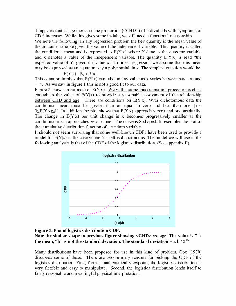
E(Y|x)= β0 + β1x. This equation implies that E(Y|x) can take on any value as x varies between say – ∞ and + ∞. As we saw in figure 1 this is not a good fit to our data. Figure 2 shows an estimate of E(Y|x). We will assume this estimation procedure is close enough to the value of E(Y|x) to provide a reasonable assessment of the relationship between CHD and age. There are conditions on E(Y|x). With dichotomous data the conditional mean must be greater than or equal to zero and less than one. [i.e. 0≤E(Y|x)≤1]. In addition the plot shows that E(Y|x) approaches zero and one gradually. The change in E(Y|x) per unit change in x becomes progressively smaller as the conditional mean approaches zero or one. The curve is S-shaped. It resembles the plot of the cumulative distribution function of a random variable. It should not seem surprising that some well-known CDFs have been used to provide a model for E(Y|x) in the case where Y itself is dichotomous. The model we will use in the following analyses is that of the CDF of the logistics distribution. (See appendix E)

logistics distribution

0

0.2

0.4

0.6

0.8

1

1.2

-6 -4 -2 0 2 4 6

(x-a)/b

CD

F

Figure 3. Plot of logistics distribution CDF. Note the similar shape to previous figure showing <CHD> vs. age. The value “a” is the mean, “b” is not the standard deviation. The standard deviation = π b / 31/2. Many distributions have been proposed for use in this kind of problem. Cox [1970] discusses some of these. There are two primary reasons for picking the CDF of the logistics distribution. First, from a mathematical viewpoint, the logistics distribution is very flexible and easy to manipulate. Second, the logistics distribution lends itself to fairly reasonable and meaningful physical interpretation.

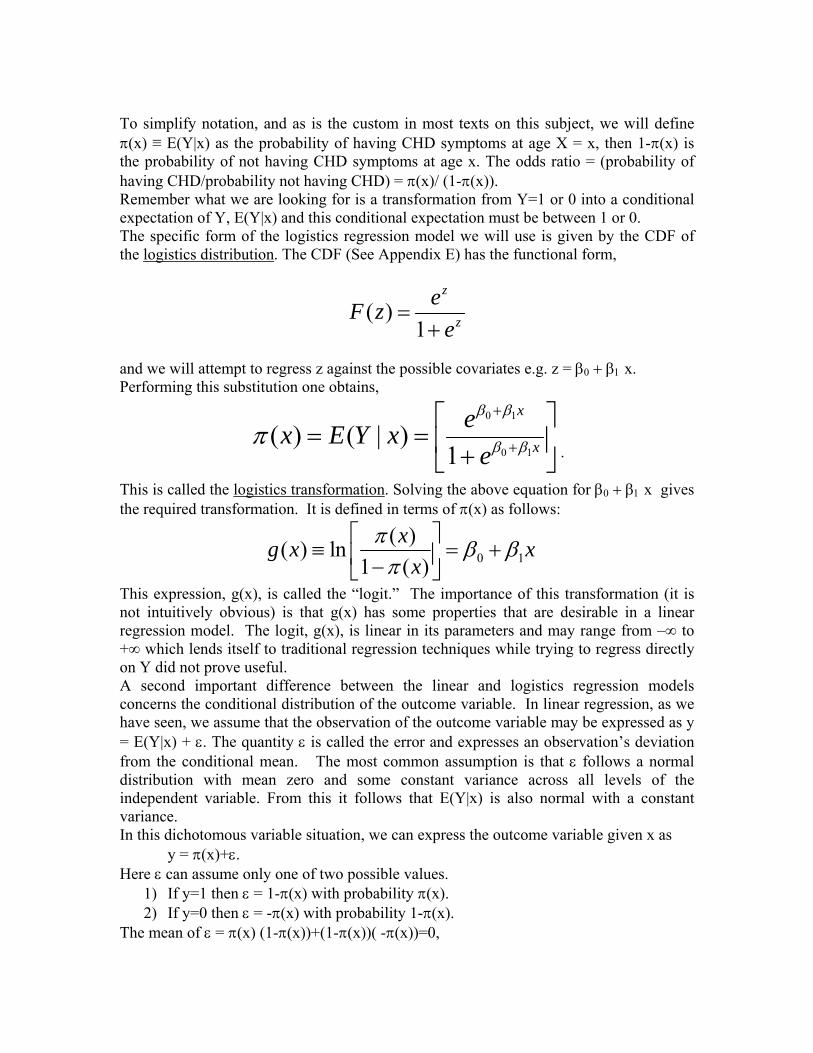
To simplify notation, and as is the custom in most texts on this subject, we will define π(x) ≡ E(Y|x) as the probability of having CHD symptoms at age X = x, then 1-π(x) is the probability of not having CHD symptoms at age x. The odds ratio = (probability of having CHD/probability not having CHD) = π(x)/ (1-π(x)). Remember what we are looking for is a transformation from Y=1 or 0 into a conditional expectation of Y, E(Y|x) and this conditional expectation must be between 1 or 0. The specific form of the logistics regression model we will use is given by the CDF of the logistics distribution. The CDF (See Appendix E) has the functional form,

( )1

z

z

eF ze

=+

and we will attempt to regress z against the possible covariates e.g. z = β0 + β1 x. Performing this substitution one obtains,

0 1

0 1( ) ( | )

1

x

xex E Y x

e

β β

β βπ+

+

⎡ ⎤= = ⎢ ⎥+⎣ ⎦ .

This is called the logistics transformation. Solving the above equation for β0 + β1 x gives the required transformation. It is defined in terms of π(x) as follows:

0 1( )( ) ln

1 ( )xg x x

xπ β β

π⎡ ⎤

≡ =⎢ ⎥−⎣ ⎦+

This expression, g(x), is called the “logit.” The importance of this transformation (it is not intuitively obvious) is that g(x) has some properties that are desirable in a linear regression model. The logit, g(x), is linear in its parameters and may range from –∞ to +∞ which lends itself to traditional regression techniques while trying to regress directly on Y did not prove useful. A second important difference between the linear and logistics regression models concerns the conditional distribution of the outcome variable. In linear regression, as we have seen, we assume that the observation of the outcome variable may be expressed as y = E(Y|x) + ε. The quantity ε is called the error and expresses an observation’s deviation from the conditional mean. The most common assumption is that ε follows a normal distribution with mean zero and some constant variance across all levels of the independent variable. From this it follows that E(Y|x) is also normal with a constant variance. In this dichotomous variable situation, we can express the outcome variable given x as

y = π(x)+ε. Here ε can assume only one of two possible values.

1) If y=1 then ε = 1-π(x) with probability π(x). 2) If y=0 then ε = -π(x) with probability 1-π(x).

The mean of ε = π(x) (1-π(x))+(1-π(x))( -π(x))=0,

The variance of ε =Var[ε]= π(x) (1-π(x))2+( 1-π(x))( -π(x))2 = π(x) (1-π(x)). Thus ε has a distribution with mean = 0 and variance = π(x)(1-π(x)) thus ε has a binomial distribution and therefore so is Y. Not surprising. If the probability π is a function of X then this violates one of the fundamental assumptions of SLR analysis so one cannot use simple least squares techniques to solve the regression problem. One uses maximum likelihood estimation (MLE) techniques instead (see below). In summary, when the outcome or response variable is dichotomous, (1) the conditional mean of the regression equation must be formulated in such a way that it is bounded between 0 and 1, (2) the binomial not the normal distribution describes the distribution of errors and will be the statistical distribution upon which the analysis is based, and (3) the principles that guide an analysis using linear regression will also guide us in logistics regression.

Fitting the Logistics Regression Model. Take a sample of data composed of n independent measurements of Y at selected values of X. These pairs (xi,yi), I=1,2,…,n, where yi denotes the value of the dichotomous outcome variable and xi is the value of the independent variable for the ith trial or test or subject. Assume the outcome variable has been coded to be either a zero or a one. We now need to determine the values of the coefficients β0 and β1 (in this simple linear model). These are the unknown parameters in this problem. Since the SLR regression techniques cannot be used, I will use a technique called the maximum likelihood estimator (MLE) method. In this MLE technique of estimating the unknown parameters one constructs the probability of actually obtaining the outcomes (yi|xi), this is called the likelihood function, and then one maximizes this likelihood function with respect to the parameters b0 and b1 using calculus. The resulting estimators are those that agree most closely with the observed data. Likelihood function. To construct a likelihood function one must recall a basic rule for probabilities. If one has two events say y1 and y2, then the probability of both events y1 and y2 occurring is given by P(y1 and y2)=P(y1)P(y2) if the two events are independent of one another. This is called the product rule for probabilities. If we have n independent events whose probabilities of occurring are θ(x1), θ(x2), …,θ(xn), then the product of all these

probabilities is called a likelihood function, . ( )1

n

ii

Likelihood xθ=

= ∏How would one construct such a function for this dichotomous outcome problem? Given that Y is coded as zero or one then the expression for π(x) provides the conditional probability that Y=1 given x. This will be denoted P(Y=1|x). It follows that the quantity1-π(x) gives the probability that Y=0 given x, denoted by P(Y=0|x). Therefore for those pairs (xi,yi) where yi=1 the contribution to the likelihood function is π(xi), and for those pairs where yi=0 the contribution to the likelihood is 1-π(xi), where π(xi) denotes the value of π(x) at xi. The probability for any single observation is given by

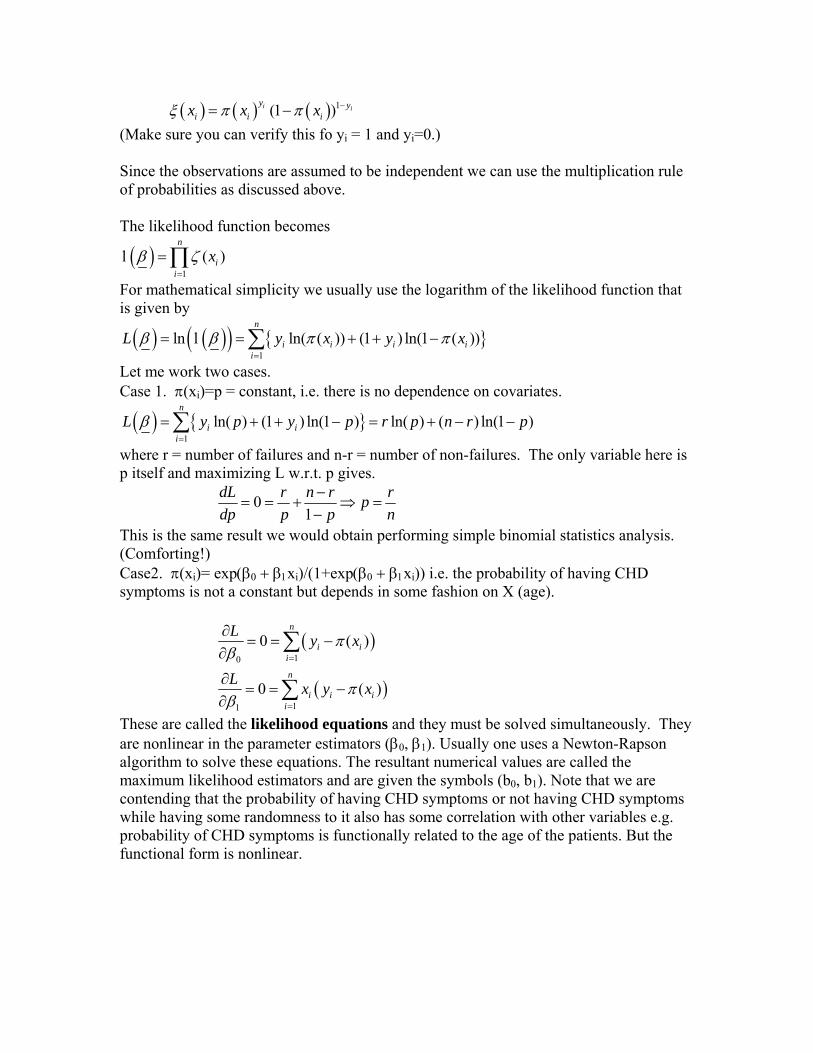
( ) ( ) ( ) 1(1 )i iy y

i i ix x xξ π π −= − (Make sure you can verify this fo yi = 1 and yi=0.) Since the observations are assumed to be independent we can use the multiplication rule of probabilities as discussed above. The likelihood function becomes

( )1

( )n

ii

xβ ζ=

= ∏l

For mathematical simplicity we usually use the logarithm of the likelihood function that is given by

( ) ( )( ) { }1

ln ln( ( )) (1 ) ln(1 ( ))n

i i i ii

L y x yβ β π π=

= = + + −∑l x

Let me work two cases. Case 1. π(xi)=p = constant, i.e. there is no dependence on covariates.

( ) { }1

ln( ) (1 ) ln(1 ) ln( ) ( ) ln(1 )n

i ii

L y p y p r p n rβ=

= + + − = + −∑ p−

where r = number of failures and n-r = number of non-failures. The only variable here is p itself and maximizing L w.r.t. p gives.

01

dL r n r rpdp p p n

−= = + ⇒ =

−

This is the same result we would obtain performing simple binomial statistics analysis. (Comforting!) Case2. π(xi)= exp(β0 + β1xi)/(1+exp(β0 + β1xi)) i.e. the probability of having CHD symptoms is not a constant but depends in some fashion on X (age).

( )

( )

10

11

0 (

0 (

n

i ii

n

i i ii

L y x

L

)

)x y x

πβ

πβ

=

=

∂= = −

∂

∂= = −

∂

∑

∑

These are called the likelihood equations and they must be solved simultaneously. They are nonlinear in the parameter estimators (β0, β1). Usually one uses a Newton-Rapson algorithm to solve these equations. The resultant numerical values are called the maximum likelihood estimators and are given the symbols (b0, b1). Note that we are contending that the probability of having CHD symptoms or not having CHD symptoms while having some randomness to it also has some correlation with other variables e.g. probability of CHD symptoms is functionally related to the age of the patients. But the functional form is nonlinear.

There are some interesting properties of these maximum likelihood estimators.

1 1( )

n n

i ii i

y xπ= =

=∑ ∑ )

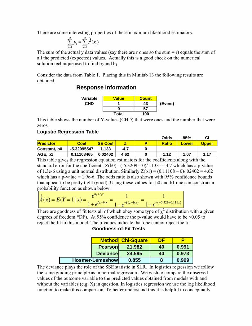
The sum of the actual y data values (say there are r ones so the sum = r) equals the sum of all the predicted (expected) values. Actually this is a good check on the numerical solution technique used to find b0 and b1. Consider the data from Table 1. Placing this in Minitab 13 the following results are obtained.

Response Information

Variable Value CountCHD 1 43 (Event)

0 57Total 100

This table shows the number of Y-values (CHD) that were ones and the number that were zeros. Logistic Regression Table Odds 95% CI Predictor Coef SE Coef Z P Ratio Lower Upper Constant, b0 -5.32095547 1.133 -4.7 0 AGE, b1 0.11108465 0.02402 4.62 0 1.12 1.07 1.17 This table gives the regression equation estimators for the coefficients along with the standard error for the coefficient. Z(b0)= (-5.3209 – 0)/1.133 = -4.7 which has a p-value of 1.3e-6 using a unit normal distribution. Similarly Z(b1) = (0.11108 – 0)/.02402 = 4.62 which has a p-value = 1.9e-6. The odds ratio is also shown with 95% confidence bounds that appear to be pretty tight (good). Using these values for b0 and b1 one can construct a probability function as shown below.

( ) ( )

0 1

0 1 0 1 5.321 0.111

1 1( ) ( 1| )1 11

b b x

b b x xb b x

ex E Y xe ee

π+

+ − − +− += = = = =

+ ++)

There are goodness of fit tests all of which obey some type of χ2 distribution with a given degrees of freedom *DF). At 95% confidence the p-value would have to be <0.05 to reject the fit to this model. The p-values indicate that one cannot reject the fit

Goodness-of-Fit Tests

Method Chi-Square DF P0.990785869 Pearson 21.982 40 0.9910.97348832 Deviance 24.595 40 0.973

Hosmer-Lemeshow 0.855 8 0.999 The deviance plays the role of the SSE statistic in SLR. In logistics regression we follow the same guiding principle as in normal regression. We wish to compare the observed values of the outcome variable to the predicted values obtained from models with and without the variables (e.g. X) in question. In logistics regression we use the log likelihood function to make this comparison. To better understand this it is helpful to conceptually

think of an observed response variable as also being a predicted value from saturated model. A saturated model is one that contains as many parameters as there are data points. The comparison of observed to predicted values of the likelihood function is based on the expression

likelihood of the current model2 lnlikelihood of the saturated model

D ⎧ ⎫= − ⎨ ⎬⎩ ⎭

D is called the deviance. The quantity inside the curly brackets is called the likelihood ratio. The reason for the –2 and taking the natural log is to transform this ratio into a quantity that has a known distribution that we can use for hypothesis testing. Such a test is called a likelihood ratio test. Using the previous equations we can express D in the following form.

1

12 ln (1 ) ln1

ni i

i ii i i

D y yy yπ π

=

⎡ ⎤⎛ ⎞ ⎛ ⎞−= − + −⎢ ⎥⎜ ⎟ ⎜ ⎟−⎢ ⎥⎝ ⎠ ⎝ ⎠⎣ ⎦

∑) )

,

i

and ( )i xπ π=) ) . For comparison purposes one wishes to know the significance of adding or subtracting from the model various independent variables e.g. X. One can do this by comparing D with and with out the variable in question. To do this the variable G is constructed where G=D(model w/o the variable) – D(model with the variable) so G has the form

likelihood without the variable2lnlikelihood with the variable

G ⎧ ⎫= − ⎨ ⎬⎩ ⎭

For the specific case given in table 1 where there is only one independent variable to test, it is easy to show that the model w/o the variable has an MLE estimate for b0 given by ln(n1/n0) where n1 = iy∑ and n0 = (1 )iy−∑ and that the predicted value p =n1/n. (see case 1). Using this one can construct G as follows:

( )

01

i

nn01

n1y

ii=1

nnn n2ln

1 iyi

Gπ π −

⎧ ⎫⎛ ⎞⎛ ⎞⎪ ⎪⎜ ⎟ ⎜ ⎟⎪ ⎪⎝ ⎠ ⎝ ⎠= − ⎨ ⎬⎪ ⎪−⎪ ⎪⎩ ⎭∏ ) )

[ ] [ 1 1 0 01

2 ln( ) (1 ) ln(1 ) ln( ) ln( ) ln( )n

i i i ii

G y y n n n n n nπ π=

⎧ ⎫= + − − − + −⎨ ⎬

⎩ ⎭∑ ) ) ]

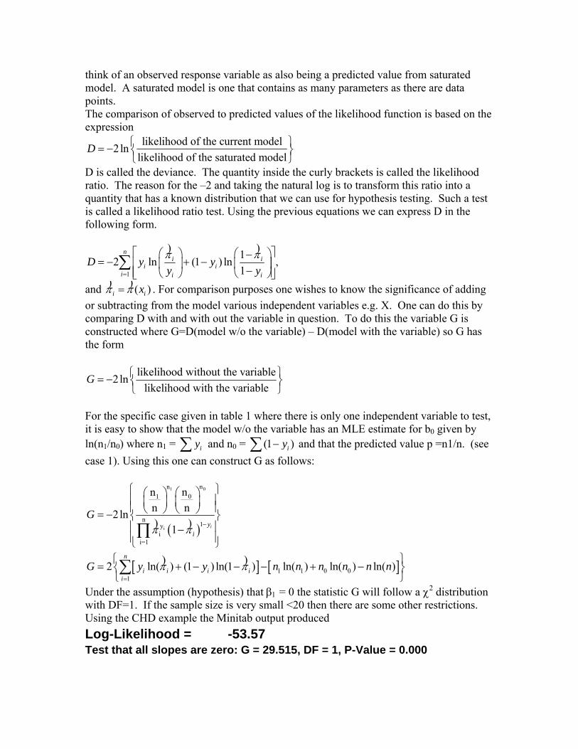
Under the assumption (hypothesis) that β1 = 0 the statistic G will follow a χ2 distribution with DF=1. If the sample size is very small <20 then there are some other restrictions. Using the CHD example the Minitab output produced Log-Likelihood = -53.57 Test that all slopes are zero: G = 29.515, DF = 1, P-Value = 0.000

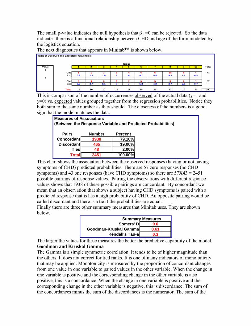
The small p-value indicates the null hypothesis that β1 =0 can be rejected. So the data indicates there is a functional relationship between CHD and age of the form modeled by the logistics equation. The next diagnostics that appears in Minitab™ is shown below. Table of Observed and Expected Frequencies:

GroupValue 1 2 3 4 5 6 7 8 9 10 Total

1ObsExp 0.8 1.3 1.9 3 4 4.7 5.8 9.3 7.9 4.3

0ObsExp 9.2 8.7 8.1 8 7 5.3 4.2 3.7 2.1 0.7

10 10 10 11 11 10 10 13 10 5 100

1 1 2 3 4 5 5 10 8 4 43

9 9 8 8 7 5 5 3 2 1 57

Total

This is comparison of the number of occurrences observed of the actual data (y=1 and y=0) vs. expected values grouped together from the regression probabilities. Notice they both sum to the same number as they should. The closeness of the numbers is a good sign that the model matches the data.

Measures of Association:(Between the Response Variable and Predicted Probabilities)

Pairs Number PercentConcordant 79.10%Discordant 19.00%

Ties 2.00%100.00%

193846548

Total 2451 This chart shows the association between the observed responses (having or not having symptoms of CHD) predicted probabilities. There are 57 zero responses (no CHD symptoms) and 43 one responses (have CHD symptoms) so there are 57X43 = 2451 possible pairings of response values. Pairing the observations with different response values shows that 1938 of these possible pairings are concordant. By concordant we mean that an observation that shows a subject having CHD symptoms is paired with a predicted response that is has a high probability of CHD. An opposite pairing would be called discordant and there is a tie if the probabilities are equal. Finally there are three other summary measures that Minitab uses. They are shown below.

Summary MeasuresSomers' D

Goodman-Kruskal GammaKendall's Tau-a

0.60.610.3

The larger the values for these measures the better the predictive capability of the model. Goodman and Kruskal Gamma The Gamma is a simple symmetric correlation. It tends to be of higher magnitude than the others. It does not correct for tied ranks. It is one of many indicators of monotonicity that may be applied. Monotonicity is measured by the proportion of concordant changes from one value in one variable to paired values in the other variable. When the change in one variable is positive and the corresponding change in the other variable is also positive, this is a concordance. When the change in one variable is positive and the corresponding change in the other variable is negative, this is discordance. The sum of the concordances minus the sum of the discordances is the numerator. The sum of the

concordances and the sum of the discordances is the total number of relations. This is the denominator. Hence, the statistic is the proportion of concordances to the total number of relations.

Kendall's Tau a For symmetric tables, Kendall noted that the number of concordances minus the number of discordances is compared to the total number of pairs, n(n-1)/2, this statistic is the Kendall's Tau a:

ID AGRP AGE CHD ID AGRP AGE CHD1 1 20 0 51 4 442 1 23 0 52 4 443 1 24 0 53 5 454 1 25 0 54 5 455 1 25 1 55 5 466 1 26 0 56 5 467 1 26 0 57 5 478 1 28 0 58 5 479 1 28 0 59 5 47

10 1 29 0 60 5 4811 2 30 0 61 5 4812 2 30 0 62 5 4813 2 30 0 63 5 4914 2 30 0 64 5 4915 2 30 0 65 5 4916 2 30 1 66 6 5017 2 32 0 67 6 5018 2 32 0 68 6 5119 2 33 0 69 6 5220 2 33 0 70 6 5221 2 34 0 71 6 5322 2 34 0 72 6 5323 2 34 1 73 6 5524 2 34 0 74 7 5525 2 34 0 75 7 5626 3 35 0 76 7 5627 3 35 0 77 7 5628 3 36 0 78 7 5629 3 36 1 79 7 5630 3 36 0 80 7 5731 3 37 0 81 7 5732 3 37 1 82 7 5733 3 37 0 83 7 5734 3 38 0 84 7 5735 3 38 0 85 7 5736 3 39 0 86 7 5837 3 39 1 87 7 5838 4 40 0 88 7 5839 4 40 1 89 7 5940 4 41 0 90 7 5941 4 41 0 91 8 6042 4 42 0 92 8 6043 4 42 0 93 8 6144 4 42 0 94 8 6245 4 42 1 95 8 6246 4 43 0 96 8 6347 4 43 0 97 8 6448 4 43 1 98 8 6449 4 44 0 99 8 6550 4 44 0 100 8 69 1

1101010010110010100111101111100111101111011111011

Table 1.1 H&L page 3

References: [1] D.C. Montgomery, E.A. Peck, G.G. Vining,(2006), Introduction to Linear Regression Analysis, 4th edition, Wiley-Interscience Publication. [2] D.N. Gujarati, (2009, paperback), Basic Econometrics, 4rd edition, McGraw-Hill. [3] T.W. Anderson,(1984), An Introduction to Multivariate Statistical Analysis, 2nd edition, John Wiley & Sons. [4] D.J. Sheskin, (1997), Handbook of Parametric & Nonparametric Statistical Procedures. CRC Press. [5] Neter, Kutner, Nachtsheim & Wasserman,(1996), Applied Linear Statistical Models, 4th edition, Irwin Pub. Co.. [6] Hahn & Shapiro, (1994), Statistical Models in Engineering, Wiley Classics Library. [7] F.A. Graybill, H.K. Iyer, (1994), Regression Analysis, Duxbury Press. [8] D.W. Hosmer, S. Lemeshow, (2000), Applied Logistic Regression, 2nd Ed., Wiley. [9] F.C. Pampel,(2000), Logistic Regression: A Primer, SAGE Publications #132. [10] N.R. Draper, D. Smith, (1998), Applied Regression Analysis, 3rd Edition.Wiley [11] Tabachnick & Fidell (1989), Using Multivariate Statistics, 2nd Edition. New York: HarperCollins. (See Appendix F)

Appendices: Appendix A: Assumptions on Liner Regression Model and the Method of Least Squares: We wish to explore the simple linear regression model and what is actually being assumed when one uses the method of least squares to solve for the coefficients (parameter estimators). Definition: The first item that needs definition is the word “linear.” Linear can have two meanings when it comes to a regression model. The first and perhaps most natural meaning of linearity is that the conditional expectation of y, i.e. , is a linear ]|[ jXYEfunction of variable Xj. Geometrically this curve would be a straight line on a y vs. xj plot. Using this interpretation, would not be a linear function 2

20]|[ jj XXYE ββ +=because the regressor variable Xj appears with a power index of 2. The second interpretation of linearity, and the one most used in this business, is that E[y|x] is a linear function of the parameters Λ,,, 210 βββ and it may or may not be linear in the x variables. The model is linear under this definition but 2

20 jXββ +]|[ jXYE =

the model jX2jXYE 0]|[ ββ += is not linear. We shall always use linear to mean linear in the parameters (or regressor coefficients) and it may or may not be linear in the regressor variables themselves. Least squares estimators (numerical properties): When using the least squares solution process to find the coefficients b0 and b1 for the equation one needs to first note the following numerical properties of these coefficients.

XbbXYE 10]|[ +=

1) The coefficients are expressed solely in terms of the observable data (X and Y). 2) The coefficients b0 and b1 are “point estimators.” That is, given a set of data (sample), there is only a single value produced for b0 and a single value for b1. 3) Once the estimates are obtained from the sample data the regression line is easily computed and it has the properties that the line passes through the sample means ),( xy . Also one notes the mean value for the estimated y, y is equal to the mean of the actual y. i.e. yy =ˆ . 4) Following from this is the mean value of the residuals is zero, i.e.

( ) 0)(ˆ1

1

1

1 =−= ∑∑==

n

jjjn

n

jjn xyye .

5) The residuals, ej, are uncorrelated with the predicted y, yj, 0ˆ1

1 =∑=

n

jjjn ey .

6) The residuals, ej, are uncorrelated with the regressor variables xj, . 01

=∑=

n

jjjex

We are now in a position to address the assumptions underlying the method of least squares. Least squares estimators (statistical properties):

Remember our objective in developing a model is to not only estimate 10 , ββ but to also draw inferences about the true 10 , ββ . How close is b1 to 1β ? How close is to the actual E[y|xj]?

)jx(y

Least squares estimators (statistical properties): The corner stone of most theory using SLR is the Gaussian standard, or classical linear regression model (CLRM) which carries with it the follow ten assumptions. Assumption 1: The regression model is linear in the parameters Λ,,, 210 βββ etc. Assumption 2: Values taken by the regressor variable(s) X are considered fixed in repeated samples. The x values are under the control of the analyst and can be inserted with arbitrary accuracy into the problem. More technically x is assumed to be non-stochastic. Assumption 3: Given a value of X=xi, the mean or expected value of the error ε is zero. (Note: this is not the residual e, which is an estimator of ε). Technically the conditional mean of ε is zero, E[ε|xi]=0. Assumption 4: Given the value of X, the variance of ε is the same for all observations. This is called homoscedasticity. In symbols . This assumptions is often violated which causes the analyst to transform the data so the variance in this transformed space is homoscedastic.

22 ]|[)|var( σεε == iiii xEx

Assumption 5: No serial correlation (autocorrelation) between the errors. 0),|,cov( =jiji xxεε . Given any two values of the regressor variable x, the correlation

between their respective error terms is zero. This means that given an Xi the deviations of any two Y values from their mean value do not exhibit patterns. Assumption 6: Zero covariance between εi and Xi, or E[εiXi]=0. Symbolically

)assumption(by 0)|cov( =ii xε and this needs to be tested. Assumption 7: The number of observations, n, must be greater than the number of parameters to be estimated. The development of the technique of partial least squares (PLS) finds its way around this restriction. Assumption 8: The X values in a given sample musty not all be the same. Technically this means that . Computing Sxx to find b1 should not produce an infinite value for b1.

0 and finite)var( >=x

Assumption 9: Regression model is correctly specified and there is no specification bias or error in the model used for the analysis. If the actual best fit model is

jj X

xy 1)(ˆ 21 ββ += and we are trying to fit with an equation of the form

jj Xxy 21)(ˆ αα += then we will not enjoy the fruits of our labor as the formulation will not be accurate. This use of a wrong model is called specification error. Assumption 10: There is no perfect multicollinearity. No perfect linear relationship between the regressor (explanatory) variables. How realistic are these assumptions? There is no general answer to this question because models always simplify the truth. If the model is useful in your understanding of the problem at hand then the realism of the assumptions may not be all that important.

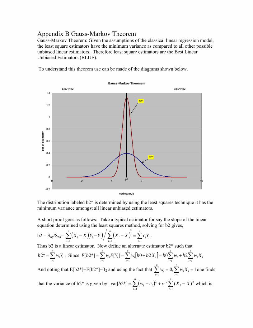
Appendix B Gauss-Markov Theorem Gauss-Markov Theorem: Given the assumptions of the classical linear regression model, the least square estimators have the minimum variance as compared to all other possible unbiased linear estimators. Therefore least square estimators are the Best Linear Unbiased Estimators (BLUE). To understand this theorem use can be made of the diagrams shown below.

Gauss-Markov Theomem

-0.2

0

0.2

0.4

0.6

0.8

1

1.2

1.4

0 2 4 6 8 10

estimator, b

pdf o

f est

imat

or

E[b2^]=β2E[b2*]=β2

β2

b2^

b2*

The distribution labeled b2^ is determined by using the least squares technique it has the minimum variance amongst all linear unbiased estimators. A short proof goes as follows: Take a typical estimator for say the slope of the linear equation determined using the least squares method, solving for b2 gives,

b2 = Sxy/Sxx= ( )( ) ( ) ∑∑∑===

=−−−n

iii

n

iii

n

ii YcXXYYXX

1

2

11.

Thus b2 is a linear estimator. Now define an alternate estimator b2* such that

. Since ∑=

=n

iiiYwb

1

*2 [ ] ∑∑∑∑====

+=+==n

iii

n

ii

n

iii

n

iii XwbwbXbbwYEwbE

1111

2020][*]2[

And noting that E[b2*]=E[b2^]=β2 and using the fact that one finds

that the variance of b2* is given by:

1,011

== ∑∑==

n

iii

n

ii Xww

( ) ∑∑==

−+−=n

ii

n

iii XXcwb

1

22

1

2 )(*]2var[ σ which is

minimized by choosing wi=ci which means that the weighting factor for b2* is the same as that for the least squares method. QED. Appendix C Multivariate regression matrices

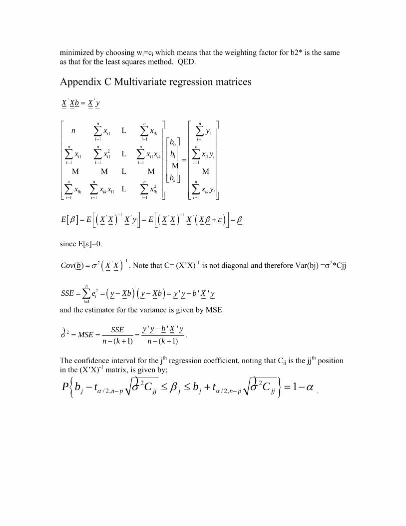
' 'X Xb X y=

11 1

02

1 1 1 111 1 1 1

21

1 1 1 1

n n n

i iki i i

n n n n

i i i ik ii i i i

kn n n n

ik ik i ik ik ii i i i

n x x yb 1

i

ix x x x b

b

x y

x x x x x y

= = =

= = = =

= = = =

⎡ ⎤⎢ ⎥⎢ ⎥ ⎡ ⎤⎢ ⎥ ⎢ ⎥⎢ ⎥ ⎢ ⎥ =⎢ ⎥ ⎢ ⎥⎢ ⎥ ⎢ ⎥

⎢ ⎥⎢ ⎥ ⎣ ⎦⎢ ⎥⎢ ⎥⎣ ⎦

∑ ∑ ∑

∑ ∑ ∑ ∑

∑ ∑ ∑ ∑

L

LM

M M L M M

L

⎡ ⎤⎢ ⎥⎢ ⎥⎢ ⎥⎢ ⎥⎢ ⎥⎢ ⎥⎢ ⎥⎢ ⎥⎢ ⎥⎣ ⎦

[ ] ( ) ( ) ( )1 1' ' ' 'E E X X X y E X X X Xβ β ε β− −⎡ ⎤ ⎡= = +⎢ ⎥ ⎢⎣ ⎦ ⎣

⎤ =⎥⎦

since E[ε]=0.

( ) 12 '( )Cov b X Xσ−

= . Note that C= (X’X)-1 is not diagonal and therefore Var(bj) =σ2*Cjj

( ) ( )'2

1' ' '

n

ii

SSE e y Xb y Xb y y b X y=

= = − − = −∑

and the estimator for the variance is given by MSE.

2 ' ' '( 1) ( 1)

y y b X ySSEMSEn k n k

σ−

= = =− + − +

) .

The confidence interval for the jth regression coefficient, noting that Cjj is the jjth position in the (X’X)-1 matrix, is given by;

{ }2 2/ 2, / 2, 1j n p jj j j n p jjP b t C b t Cα ασ β σ− −− ≤ ≤ +) ) α= − .

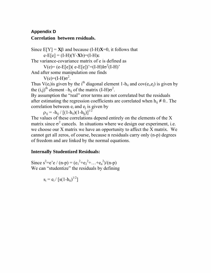
Appendix D Correlation between residuals. Since E[Y] = Xβ and because (I-H)X=0, it follows that e-E[e] = (I-H)(Y-Xb)=(I-H)ε The variance-covariance matrix of e is defined as V(e)= (e-E[e])( e-E[e])’=(I-H)Iσ2(I-H)’ And after some manipulation one finds V(e)=(I-H)σ2. Thus V(ei)is given by the ith diagonal element 1-hii and cov(ei,ej) is given by the (i,j)th element –hij of the matrix (I-H)σ2. By assumption the “real” error terms are not correlated but the residuals after estimating the regression coefficients are correlated when hij ≠ 0.. The correlation between ei and ej is given by ρij = -hij / [(1-hii)(1-hjj)]1/2 The values of these correlations depend entirely on the elements of the X matrix since σ2 cancels. In situations where we design our experiment, i.e. we choose our X matrix we have an opportunity to affect the X matrix. We cannot get all zeros, of course, because n residuals carry only (n-p) degrees of freedom and are linked by the normal equations. Internally Studentized Residuals: Since s2=e’e / (n-p) = (e1

2+e22+…+en

2)/(n-p) We can “studentize” the residuals by defining si = ei / [s(1-hii)1/2]

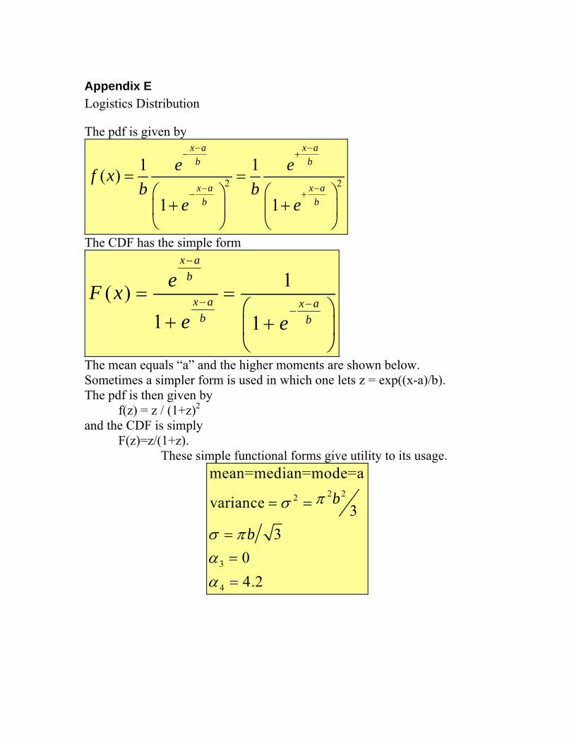
Appendix E Logistics Distribution The pdf is given by

2 21 1( )

1 1

x a x ab b

x a x ab b

e ef xb b

e e

− −− +

− −− +

= =⎛ ⎞ ⎛

+ +⎜ ⎟ ⎜⎝ ⎠ ⎝

⎞⎟⎠

The CDF has the simple form

1( )1 1

x ab

x a x ab b

eF xe e

−

− −−

= =⎛ ⎞

+ +⎜ ⎟⎝ ⎠

The mean equals “a” and the higher moments are shown below. Sometimes a simpler form is used in which one lets z = exp((x-a)/b). The pdf is then given by

f(z) = z / (1+z)2 and the CDF is simply

F(z)=z/(1+z). These simple functional forms give utility to its usage.

2 22

3

4

mean=median=mode=a

variance 33

04.2

b

b

πσ

σ παα

= =

===

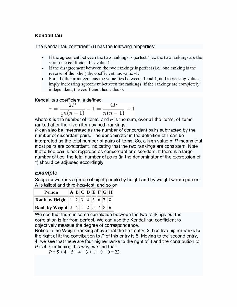
Kendall tau

The Kendall tau coefficient (τ) has the following properties:

• If the agreement between the two rankings is perfect (i.e., the two rankings are the same) the coefficient has value 1.

• If the disagreement between the two rankings is perfect (i.e., one ranking is the reverse of the other) the coefficient has value -1.

• For all other arrangements the value lies between -1 and 1, and increasing values imply increasing agreement between the rankings. If the rankings are completely independent, the coefficient has value 0.

Kendall tau coefficient is defined

where n is the number of items, and P is the sum, over all the items, of items ranked after the given item by both rankings. P can also be interpreted as the number of concordant pairs subtracted by the number of discordant pairs. The denominator in the definition of τ can be interpreted as the total number of pairs of items. So, a high value of P means that most pairs are concordant, indicating that the two rankings are consistent. Note that a tied pair is not regarded as concordant or discordant. If there is a large number of ties, the total number of pairs (in the denominator of the expression of τ) should be adjusted accordingly.

Example Suppose we rank a group of eight people by height and by weight where person A is tallest and third-heaviest, and so on:

Person A B C D E F G H

Rank by Height 1 2 3 4 5 6 7 8 Rank by Weight 3 4 1 2 5 7 8 6 We see that there is some correlation between the two rankings but the correlation is far from perfect. We can use the Kendall tau coefficient to objectively measue the degree of correspondence. Notice in the Weight ranking above that the first entry, 3, has five higher ranks to the right of it; the contribution to P of this entry is 5. Moving to the second entry, 4, we see that there are four higher ranks to the right of it and the contribution to P is 4. Continuing this way, we find that

P = 5 + 4 + 5 + 4 + 3 + 1 + 0 + 0 = 22.

Thus .

This result indicates a strong agreement between the rankings, as expected.

Goodman – Kruskal Gamma

Another non-parametric measure of correlation is Goodman – Kruskal Gamma ( Γ) which is based on the difference between concordant pairs (C) and discordant pairs (D). Gamma is computed as follows:

Γ = (C-D)/(C+D)

Thus, Gamma is the surplus of concordant pairs over discordant pairs, as a percentage of all pairs, ignoring ties. Gamma defines perfect association as weak monotonicity. Under statistical independence, Gamma will be 0, but it can be 0 at other times as well (whenever concordant minus discordant pairs are 0).

Gamma is a symmetric measure and computes the same coefficient value, regardless of which is the independent (column) variable. Its value ranges between +1 to –1.

In terms of the underlying assumptions, Gamma is equivalent to Spearman’s Rho or Kendall’s Tau; but in terms of its interpretation and computation, it is more similar to Kendall’s Tau than Spearman’s Rho. Gamma statistic is, however, preferable to Spearman’s Rho and Kandall’s Tau, when the data contain many tied observations.

Fisher's Exact Test

Fisher's exact test is a test for independence in a 2 × 2 table.. . This test is designed to test the hypothesis that the two column percentages are equal. It is particularly useful when sample sizes are small (even zero in some cells) and the Chi-square test is not appropriate. The test determines whether the two groups differ in the proportion with which they fall in two classifications: The test is based on the probability of the observed outcome, and is given by the following formula:

where a, b, c, d represent the frequencies in the four cells;. N = total number of cases.

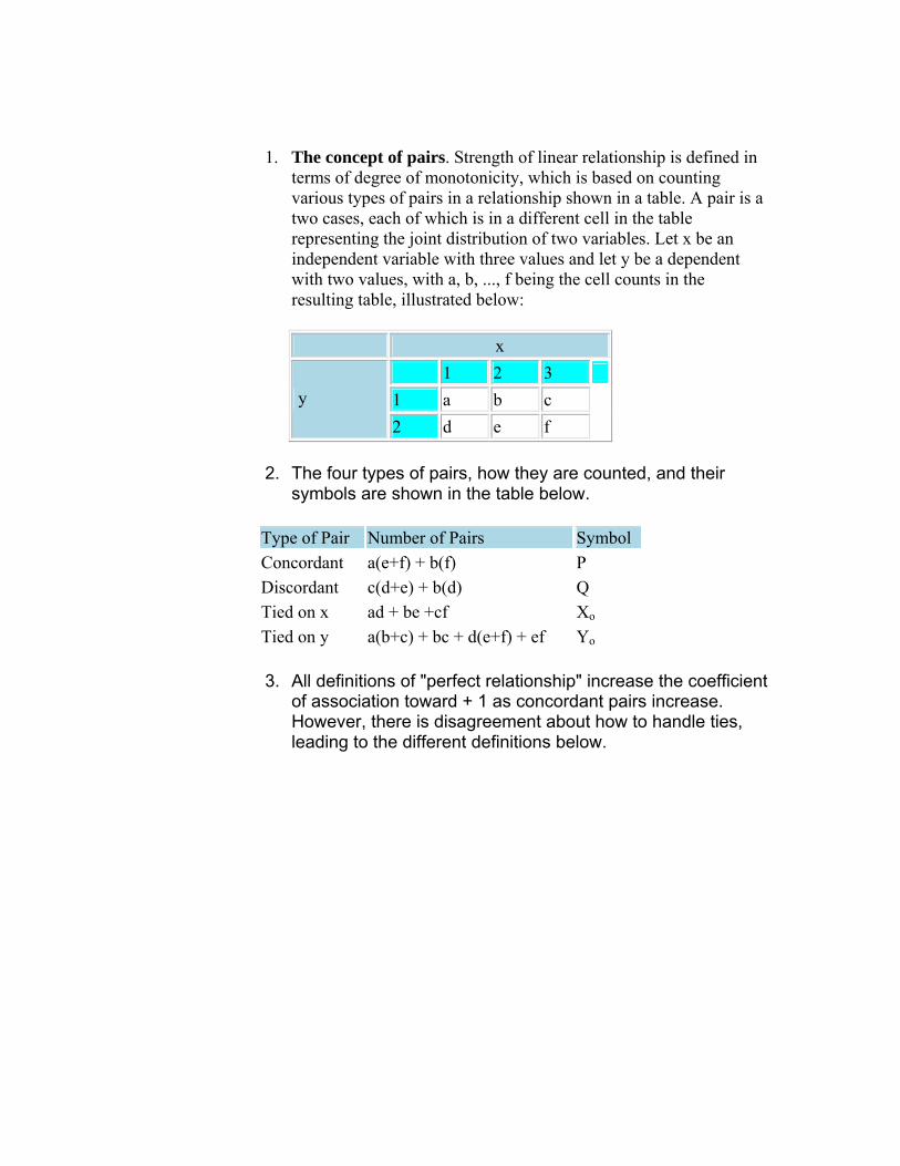
1. The concept of pairs. Strength of linear relationship is defined in terms of degree of monotonicity, which is based on counting various types of pairs in a relationship shown in a table. A pair is a two cases, each of which is in a different cell in the table representing the joint distribution of two variables. Let x be an independent variable with three values and let y be a dependent with two values, with a, b, ..., f being the cell counts in the resulting table, illustrated below:

x 1 2 3

1 a b c y 2 d e f

2. The four types of pairs, how they are counted, and their symbols are shown in the table below.

Type of Pair Number of Pairs Symbol Concordant a(e+f) + b(f) P Discordant c(d+e) + b(d) Q Tied on x ad + be +cf Xo Tied on y a(b+c) + bc + d(e+f) + ef Yo

3. All definitions of "perfect relationship" increase the coefficient of association toward + 1 as concordant pairs increase. However, there is disagreement about how to handle ties, leading to the different definitions below.

Appendix F

Assumptions of Regression (Much of this information comes from Tabachnick & Fidell (1989), Using Multivariate Statistics. (2nd Edition). New York: HarperCollins)

Number of cases

When doing regression, the number of data points-to-Independent Variables (IVs) ratio should ideally be 20:1; that is 20 data values for every IV in the model. The lowest your ratio should be is 5:1 (i.e., 5 data values for every IV in the model).

Accuracy of data

If you have entered the data (rather than using an established dataset), it is a good idea to check the accuracy of the data entry. If you don't want to re-check each data point, you should at least check the minimum and maximum value for each variable to ensure that all values for each variable are "valid." For example, a variable that is measured using a 1 to 5 scale should not have a value of 8.

Missing data

You also want to look for missing data. If specific variables have a lot of missing values, you may decide not to include those variables in your analyses. If only a few cases have any missing values, then you might want to delete those cases. If there are missing values for several cases on different variables, then you probably don't want to delete those cases (because a lot of your data will be lost). If there are not too much missing data, and there does not seem to be any pattern in terms of what is missing, then you don't really need to worry. Just run your regression, and any cases that do not have values for the variables used in that regression will not be included. Although tempting, do not assume that there is no pattern; check for this. To do this, separate the dataset into two groups: those cases missing values for a certain variable, and those not missing a value for that variable. Using t-tests, you can determine if the two groups differ on other variables included in the sample. For example, you might find that the cases that are missing values for the "salary" variable are younger than those cases that have values for salary. You would want to do t-tests for each variable with a lot of missing values. If there is a systematic difference between the two groups (i.e., the group missing values vs. the group not missing values), then you would need to keep this in mind when interpreting your findings and not over generalize.

After examining your data, you may decide that you want to replace the missing values with some other value. The easiest thing to use as the replacement value is the mean of this variable. Some statistics programs have an option within regression where you can replace the missing value with the mean. Alternatively, you may want to substitute a group mean (e.g., the mean for females) rather than the overall mean.

The default option of statistics packages is to exclude cases that are missing values for any variable that is included in regression. (But that case could be included in another regression, as long as it was not missing values on any of the variables included in that analysis.) You can change this option so that your regression analysis does not exclude cases that are missing data for any variable included in the regression, but then you might have a different number of cases for each variable.

Outliers

You also need to check your data for outliers (i.e., an extreme value on a particular item) An outlier is often operationally defined as a value that is at least 3 standard deviations above or below the mean. If you feel that the cases that produced the outliers are not part of the same "population" as the other cases, then you might just want to delete those cases. Alternatively, you might want to count those extreme values as "missing," but retain the case for other variables. Alternatively, you could retain the outlier, but reduce how extreme it is. Specifically, you might want to recode the value so that it is the highest (or lowest) non-outlier value.

Normality

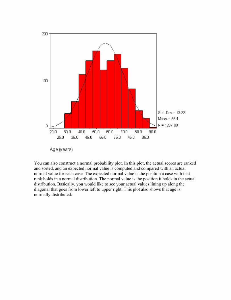
You also want to check that your data is normally distributed. To do this, you can construct histograms and "look" at the data to see its distribution. Often the histogram will include a line that depicts what the shape would look like if the distribution were truly normal (and you can "eyeball" how much the actual distribution deviates from this line). This histogram shows that age is normally distributed:

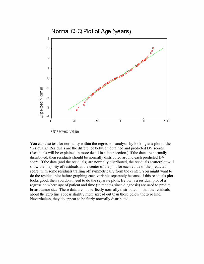
You can also construct a normal probability plot. In this plot, the actual scores are ranked and sorted, and an expected normal value is computed and compared with an actual normal value for each case. The expected normal value is the position a case with that rank holds in a normal distribution. The normal value is the position it holds in the actual distribution. Basically, you would like to see your actual values lining up along the diagonal that goes from lower left to upper right. This plot also shows that age is normally distributed:

You can also test for normality within the regression analysis by looking at a plot of the "residuals." Residuals are the difference between obtained and predicted DV scores. (Residuals will be explained in more detail in a later section.) If the data are normally distributed, then residuals should be normally distributed around each predicted DV score. If the data (and the residuals) are normally distributed, the residuals scatterplot will show the majority of residuals at the center of the plot for each value of the predicted score, with some residuals trailing off symmetrically from the center. You might want to do the residual plot before graphing each variable separately because if this residuals plot looks good, then you don't need to do the separate plots. Below is a residual plot of a regression where age of patient and time (in months since diagnosis) are used to predict breast tumor size. These data are not perfectly normally distributed in that the residuals about the zero line appear slightly more spread out than those below the zero line. Nevertheless, they do appear to be fairly normally distributed.

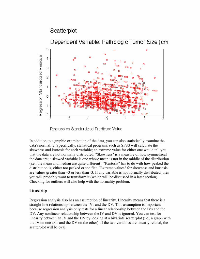
In addition to a graphic examination of the data, you can also statistically examine the data's normality. Specifically, statistical programs such as SPSS will calculate the skewness and kurtosis for each variable; an extreme value for either one would tell you that the data are not normally distributed. "Skewness" is a measure of how symmetrical the data are; a skewed variable is one whose mean is not in the middle of the distribution (i.e., the mean and median are quite different). "Kurtosis" has to do with how peaked the distribution is, either too peaked or too flat. "Extreme values" for skewness and kurtosis are values greater than +3 or less than -3. If any variable is not normally distributed, then you will probably want to transform it (which will be discussed in a later section). Checking for outliers will also help with the normality problem.

Linearity

Regression analysis also has an assumption of linearity. Linearity means that there is a straight line relationship between the IVs and the DV. This assumption is important because regression analysis only tests for a linear relationship between the IVs and the DV. Any nonlinear relationship between the IV and DV is ignored. You can test for linearity between an IV and the DV by looking at a bivariate scatterplot (i.e., a graph with the IV on one axis and the DV on the other). If the two variables are linearly related, the scatterplot will be oval.

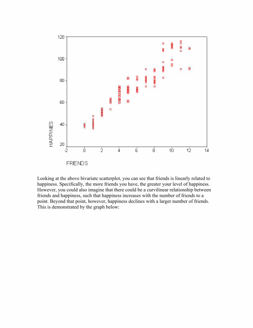
Looking at the above bivariate scatterplot, you can see that friends is linearly related to happiness. Specifically, the more friends you have, the greater your level of happiness. However, you could also imagine that there could be a curvilinear relationship between friends and happiness, such that happiness increases with the number of friends to a point. Beyond that point, however, happiness declines with a larger number of friends. This is demonstrated by the graph below:

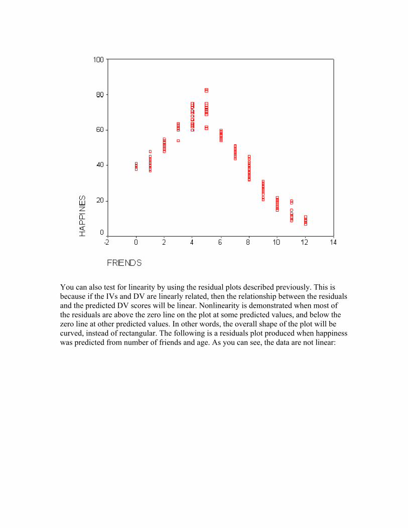
You can also test for linearity by using the residual plots described previously. This is because if the IVs and DV are linearly related, then the relationship between the residuals and the predicted DV scores will be linear. Nonlinearity is demonstrated when most of the residuals are above the zero line on the plot at some predicted values, and below the zero line at other predicted values. In other words, the overall shape of the plot will be curved, instead of rectangular. The following is a residuals plot produced when happiness was predicted from number of friends and age. As you can see, the data are not linear:

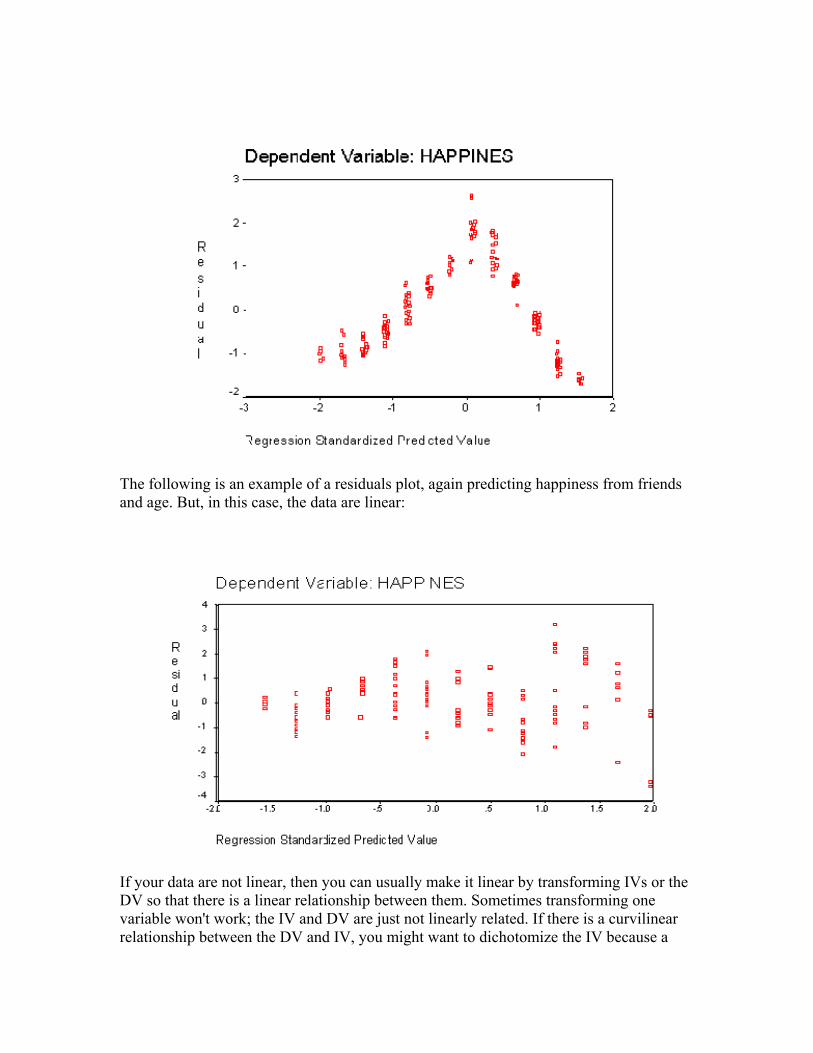
The following is an example of a residuals plot, again predicting happiness from friends and age. But, in this case, the data are linear:

If your data are not linear, then you can usually make it linear by transforming IVs or the DV so that there is a linear relationship between them. Sometimes transforming one variable won't work; the IV and DV are just not linearly related. If there is a curvilinear relationship between the DV and IV, you might want to dichotomize the IV because a

dichotomous variable can only have a linear relationship with another variable (if it has any relationship at all). Alternatively, if there is a curvilinear relationship between the IV and the DV, then you might need to include the square of the IV in the regression (this is also known as a quadratic regression).

The failure of linearity in regression will not invalidate your analysis so much as weaken it; the linear regression coefficient cannot fully capture the extent of a curvilinear relationship. If there is both a curvilinear and a linear relationship between the IV and DV, then the regression will at least capture the linear relationship.

Homoscedasticity

The assumption of homoscedasticity is that the residuals are approximately equal for all predicted DV scores. Another way of thinking of this is that the variability in scores for your IVs is the same at all values of the DV. You can check homoscedasticity by looking at the same residuals plot talked about in the linearity and normality sections. Data are homoscedastic if the residuals plot is the same width for all values of the predicted DV. Heteroscedasticity is usually shown by a cluster of points that is wider as the values for the predicted DV get larger. Alternatively, you can check for homoscedasticity by looking at a scatterplot between each IV and the DV. As with the residuals plot, you want the cluster of points to be approximately the same width all over. The following residuals plot shows data that are fairly homoscedastic. In fact, this residuals plot shows data that meet the assumptions of homoscedasticity, linearity, and normality (because the residual plot is rectangular, with a concentration of points along the center):

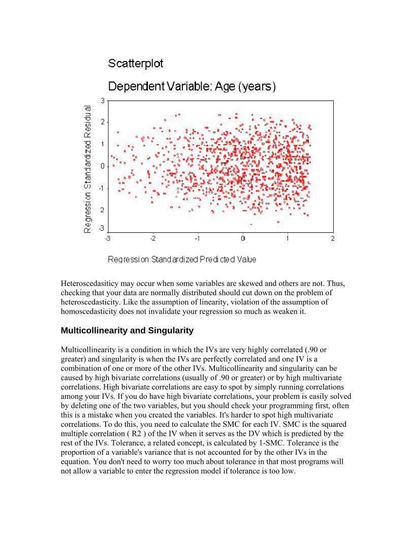
Heteroscedasiticy may occur when some variables are skewed and others are not. Thus, checking that your data are normally distributed should cut down on the problem of heteroscedasticity. Like the assumption of linearity, violation of the assumption of homoscedasticity does not invalidate your regression so much as weaken it.

Multicollinearity and Singularity

Multicollinearity is a condition in which the IVs are very highly correlated (.90 or greater) and singularity is when the IVs are perfectly correlated and one IV is a combination of one or more of the other IVs. Multicollinearity and singularity can be caused by high bivariate correlations (usually of .90 or greater) or by high multivariate correlations. High bivariate correlations are easy to spot by simply running correlations among your IVs. If you do have high bivariate correlations, your problem is easily solved by deleting one of the two variables, but you should check your programming first, often this is a mistake when you created the variables. It's harder to spot high multivariate correlations. To do this, you need to calculate the SMC for each IV. SMC is the squared multiple correlation ( R2 ) of the IV when it serves as the DV which is predicted by the rest of the IVs. Tolerance, a related concept, is calculated by 1-SMC. Tolerance is the proportion of a variable's variance that is not accounted for by the other IVs in the equation. You don't need to worry too much about tolerance in that most programs will not allow a variable to enter the regression model if tolerance is too low.

Statistically, you do not want singularity or multicollinearity because calculation of the regression coefficients is done through matrix inversion. Consequently, if singularity exists, the inversion is impossible, and if multicollinearity exists the inversion is unstable. Logically, you don't want multicollinearity or singularity because if they exist, then your IVs are redundant with one another. In such a case, one IV doesn't add any predictive value over another IV, but you do lose a degree of freedom. As such, having multicollinearity/ singularity can weaken your analysis. In general, you probably wouldn't want to include two IVs that correlate with one another at .70 or greater.

Transformations

As mentioned in the section above, when one or more variables are not normally distributed, you might want to transform them. You could also use transformations to correct for heteroscedasiticy, nonlinearity, and outliers. Some people do not like to do transformations because it becomes harder to interpret the analysis. Thus, if your variables are measured in "meaningful" units, such as days, you might not want to use transformations. If, however, your data are just arbitrary values on a scale, then transformations don't really make it more difficult to interpret the results.

Since the goal of transformations is to normalize your data, you want to re- check for normality after you have performed your transformations. Deciding which transformation is best is often an exercise in trial-and-error where you use several transformations and see which one has the best results. "Best results" means the transformation whose distribution is most normal. The specific transformation used depends on the extent of the deviation from normality. If the distribution differs moderately from normality, a square root transformation is often the best. A log transformation is usually best if the data are more substantially non-normal. An inverse transformation should be tried for severely non-normal data. If nothing can be done to "normalize" the variable, then you might want to dichotomize the variable (as was explained in the linearity section). Direction of the deviation is also important. If the data is negatively skewed, you should "reflect" the data and then apply the transformation. To reflect a variable, create a new variable where the original value of the variable is subtracted from a constant. The constant is calculated by adding 1 to the largest value of the original variable.

If you have transformed your data, you need to keep that in mind when interpreting your findings. For example, imagine that your original variable was measured in days, but to make the data more normally distributed, you needed to do an inverse transformation. Now you need to keep in mind that the higher the value for this transformed variable, the lower the value the original variable, days. A similar thing will come up when you "reflect" a variable. A greater value for the original variable will translate into a smaller value for the reflected variable.

Simple Linear Regression

Simple linear regression is when you want to predict values of one variable, given values of another variable. For example, you might want to predict a person's height (in inches)

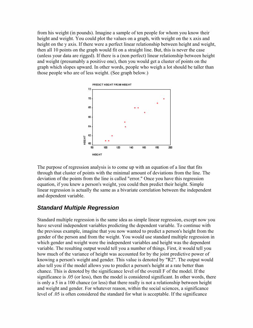
from his weight (in pounds). Imagine a sample of ten people for whom you know their height and weight. You could plot the values on a graph, with weight on the x axis and height on the y axis. If there were a perfect linear relationship between height and weight, then all 10 points on the graph would fit on a straight line. But, this is never the case (unless your data are rigged). If there is a (non perfect) linear relationship between height and weight (presumably a positive one), then you would get a cluster of points on the graph which slopes upward. In other words, people who weigh a lot should be taller than those people who are of less weight. (See graph below.)

The purpose of regression analysis is to come up with an equation of a line that fits through that cluster of points with the minimal amount of deviations from the line. The deviation of the points from the line is called "error." Once you have this regression equation, if you knew a person's weight, you could then predict their height. Simple linear regression is actually the same as a bivariate correlation between the independent and dependent variable.

Standard Multiple Regression

Standard multiple regression is the same idea as simple linear regression, except now you have several independent variables predicting the dependent variable. To continue with the previous example, imagine that you now wanted to predict a person's height from the gender of the person and from the weight. You would use standard multiple regression in which gender and weight were the independent variables and height was the dependent variable. The resulting output would tell you a number of things. First, it would tell you how much of the variance of height was accounted for by the joint predictive power of knowing a person's weight and gender. This value is denoted by "R2". The output would also tell you if the model allows you to predict a person's height at a rate better than chance. This is denoted by the significance level of the overall F of the model. If the significance is .05 (or less), then the model is considered significant. In other words, there is only a 5 in a 100 chance (or less) that there really is not a relationship between height and weight and gender. For whatever reason, within the social sciences, a significance level of .05 is often considered the standard for what is acceptable. If the significance

level is between .05 and .10, then the model is considered marginal. In other words, the model is fairly good at predicting a person's height, but there is between a 5-10% probability that there really is not a relationship between height and weight and gender.

In addition to telling you the predictive value of the overall model, standard multiple regression tells you how well each independent variable predicts the dependent variable, controlling for each of the other independent variables. In our example, then, the regression would tell you how well weight predicted a person's height, controlling for gender, as well as how well gender predicted a person's height, controlling for weight.

To see if weight was a "significant" predictor of height you would look at the significance level associated with weight on the printout. Again, significance levels of .05 or lower would be considered significant, and significance levels .05 and .10 would be considered marginal. Once you have determined that weight was a significant predictor of height, then you would want to more closely examine the relationship between the two variables. In other words, is the relationship positive or negative? In this example, we would expect that there would be a positive relationship. In other words, we would expect that the greater a person's weight, the greater his height. (A negative relationship would be denoted by the case in which the greater a person's weight, the shorter his height.) We can determine the direction of the relationship between weight and height by looking at the regression coefficient associated with weight. There are two kinds of regression coefficients: B (unstandardized) and beta (standardized). The B weight associated with each variable is given in terms of the units of this variable. For weight, the unit would be pounds, and for height, the unit is inches. The beta uses a standard unit that is the same for all variables in the equation. In our example, this would be a unit of measurement that would be common to weight and height. Beta weights are useful because then you can compare two variables that are measured in different units, as are height and weight.

If the regression coefficient is positive, then there is a positive relationship between height and weight. If this value is negative, then there is a negative relationship between height and weight. We can more specifically determine the relationship between height and weight by looking at the beta coefficient for weight. If the beta = .35, for example, then that would mean that for one unit increase in weight, height would increase by .35 units. If the beta=-.25, then for one unit increase in weight, height would decrease by .25 units. Of course, this relationship is valid only when holding gender constant.

A similar procedure would be done to see how well gender predicted height. However, because gender is a dichotomous variable, the interpretation of the printouts is slightly different. As with weight, you would check to see if gender was a significant predictor of height, controlling for weight. The difference comes when determining the exact nature of the relationship between gender and height. That is, it does not make sense to talk about the effect on height as gender increases or decreases, since gender is not a continuous variable (we would hope). Imagine that gender had been coded as either 0 or 1, with 0 = female and 1=male. If the beta coefficient of gender were positive, this would mean that males are taller than females. If the beta coefficient of gender were negative, this would mean that males are shorter than females. Looking at the magnitude of the

beta, you can more closely determine the relationship between height and gender. Imagine that the beta of gender were .25. That means that males would be .25 units taller than females. Conversely, if the beta coefficient were -.25, this would mean that males were .25 units shorter than females. Of course, this relationship would be true only when controlling for weight.

As mentioned, the significance levels given for each independent variable indicates whether that particular independent variable is a significant predictor of the dependent variable, over and above the other independent variables. Because of this, an independent variable that is a significant predictor of a dependent variable in simple linear regression may not be significant in multiple regression (i.e., when other independent variables are added into the equation). This could happen because the variance that the first independent variable shares with the dependent variable could overlap with the variance that is shared between the second independent variable and the dependent variable. Consequently, the first independent variable is no longer uniquely predictive and thus would not show up as being significant in the multiple regression. Because of this, it is possible to get a highly significant R2, but have none of the independent variables be significant.

Appendix G

Ridge Regression and the SPSS Ridge Regression Macro Ridge regression is an ad hoc solution applied to a data set that is troublesome because of multicollinearity, or high inter-correlations among scores on the independent variables. Excessive multicollinearity can cause several problems: (a) estimates of regression coefficients that are biased and don’t seem plausible, given the ordinary (zero-order) correlations of scores on single independent variables with those on the dependent variable; and (b) poor accuracy of regression computations, due to very small tolerances. Common methods for avoiding such situations include: • Dropping variables that appear to be redundant with others. • Combining variables into linear composites that are independent of others. Ridge regression involves purposely introducing error into the data set (independent variables) in order to reduce the bias in estimates of the individual regression coefficients. This is accomplished by adding a small, constant value to the main diagonal of the correlation matrix prior to performing the inversion (when all variables are standardized, as is the case in a correlation matrix, the standardized regression coefficients may be estimated by R-1r, where R is the correlation matrix for independent variables, and r is the vector of correlations of the independent variables with the dependent variable). Thus, a small “ridge” is built up, so that the values on the main diagonal tend to be larger than the values elsewhere in the correlation matrix, R. Usually, one starts with very small values, and adds successively larger ones. The goal is to choose the smallest constant value that seems to result in stable estimates of coefficients. Suppose that the matrix of correlations among three predictors was: Original Matrix (lower diagonal shown) Var1 1.00 Var2 0.85 1.00

Var3 0.92 0.90 1.00 This matrix manifests considerable redundancy among the independent variables. One measure of this situation is the value of the determinant, which is 0.029. The smaller the determinant, the less unique information or variation can be said to exist among the set of variables (or, conversely, the higher the overlap or redundancy). Now, consider the same matrix, with a ridge constant of .05 added on the main diagonal; the determinant is now 0.067. Matrix with Ridge Constant of .05 Added (lower diagonal shown):

Var1 Var2 Var3Var1 1.05Var2 0.85 1.05Var3 0.92 0.9 1.05

An Example From Longley, J. W. (1967). An appraisal of least squares programs for the electronic computer from the point of view of the user. Journal of the American Statistical Association, 62, 819-841. The Longley data set is often used as an example of a data set that manifests severe multicollinearity among the independent variables. Variables are: X1 = GNP Deflator X2 = GNP (Gross National Product) X3 = Unemployed X4 = Armed Forces X5 = U.S. Population (in millions) X6 = Year (1947-1962) Y = Employed (in millions) Correlations.

Y X1 X2 X3 X4 X5 X6Y 1 0.971 0.984 0.502 0.457 0.96 0.971X1 1 0.992 0.621 0.465 0.979 0.991X2 1 0.604 0.446 0.991 0.995X3 1 -0.177 0.687 0.668X4 1 0.364 0.417X5 1 0.994X6 1

Determinant of correlation matrix (among Xs: X1-X6) = 0.0000000016 DATA

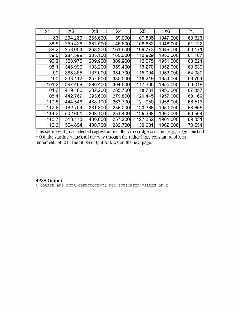
X1 X2 X3 X4 X5 X6 Y.83 234.289 235.600 159.000 107.608 1947.000 60.323

88.5 259.426 232.500 145.600 108.632 1948.000 61.12288.2 258.054 368.200 161.600 109.773 1949.000 60.17189.5 284.599 335.100 165.000 110.929 1950.000 61.18796.2 328.975 209.900 309.900 112.075 1951.000 63.22198.1 346.999 193.200 359.400 113.270 1952.000 63.639

99 365.385 187.000 354.700 115.094 1953.000 64.989100 363.112 357.800 335.000 116.219 1954.000 63.761

101.2 397.469 290.400 304.800 117.388 1955.000 66.019104.6 419.180 282.200 285.700 118.734 1956.000 67.857108.4 442.769 293.600 279.800 120.445 1957.000 68.169110.8 444.546 468.100 263.700 121.950 1958.000 66.513112.6 482.704 381.300 255.200 123.366 1959.000 68.655114.2 502.601 393.100 251.400 125.368 1960.000 69.564115.7 518.173 480.600 257.200 127.852 1961.000 69.331116.9 554.894 400.700 282.700 130.081 1962.000 70.551

This set-up will give selected regression results for no ridge constant (e.g., ridge constant = 0.0, the starting value), all the way through the rather large constant of .40, in increments of .01. The SPSS output follows on the next page. SPSS Output: R-SQUARE AND BETA COEFFICIENTS FOR ESTIMATED VALUES OF K

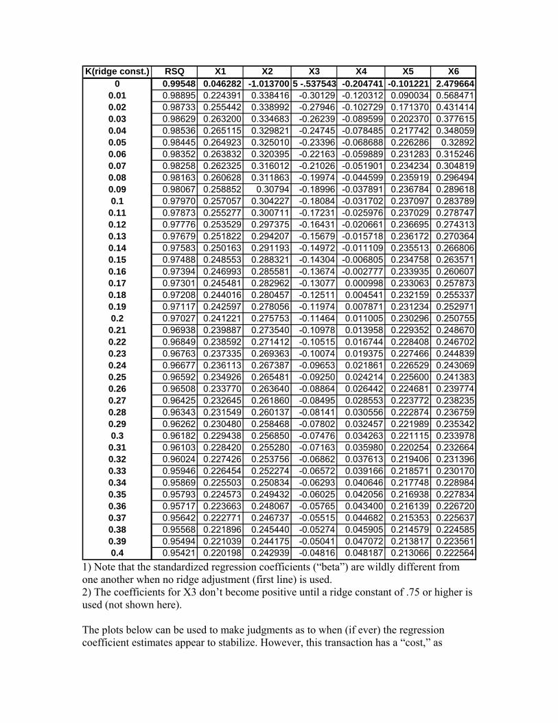
K(ridge const.) RSQ X1 X2 X3 X4 X5 X60 0.99548 0.046282 -1.013700 5 -.537543 -0.204741 -0.101221 2.479664

0.01 0.98895 0.224391 0.338416 -0.30129 -0.120312 0.090034 0.5684710.02 0.98733 0.255442 0.338992 -0.27946 -0.102729 0.171370 0.4314140.03 0.98629 0.263200 0.334683 -0.26239 -0.089599 0.202370 0.3776150.04 0.98536 0.265115 0.329821 -0.24745 -0.078485 0.217742 0.3480590.05 0.98445 0.264923 0.325010 -0.23396 -0.068688 0.226286 0.328920.06 0.98352 0.263832 0.320395 -0.22163 -0.059889 0.231283 0.3152460.07 0.98258 0.262325 0.316012 -0.21026 -0.051901 0.234234 0.3048190.08 0.98163 0.260628 0.311863 -0.19974 -0.044599 0.235919 0.2964940.09 0.98067 0.258852 0.30794 -0.18996 -0.037891 0.236784 0.2896180.1 0.97970 0.257057 0.304227 -0.18084 -0.031702 0.237097 0.283789

0.11 0.97873 0.255277 0.300711 -0.17231 -0.025976 0.237029 0.2787470.12 0.97776 0.253529 0.297375 -0.16431 -0.020661 0.236695 0.2743130.13 0.97679 0.251822 0.294207 -0.15679 -0.015718 0.236172 0.2703640.14 0.97583 0.250163 0.291193 -0.14972 -0.011109 0.235513 0.2668060.15 0.97488 0.248553 0.288321 -0.14304 -0.006805 0.234758 0.2635710.16 0.97394 0.246993 0.285581 -0.13674 -0.002777 0.233935 0.2606070.17 0.97301 0.245481 0.282962 -0.13077 0.000998 0.233063 0.2578730.18 0.97208 0.244016 0.280457 -0.12511 0.004541 0.232159 0.2553370.19 0.97117 0.242597 0.278056 -0.11974 0.007871 0.231234 0.2529710.2 0.97027 0.241221 0.275753 -0.11464 0.011005 0.230296 0.250755

0.21 0.96938 0.239887 0.273540 -0.10978 0.013958 0.229352 0.2486700.22 0.96849 0.238592 0.271412 -0.10515 0.016744 0.228408 0.2467020.23 0.96763 0.237335 0.269363 -0.10074 0.019375 0.227466 0.2448390.24 0.96677 0.236113 0.267387 -0.09653 0.021861 0.226529 0.2430690.25 0.96592 0.234926 0.265481 -0.09250 0.024214 0.225600 0.2413830.26 0.96508 0.233770 0.263640 -0.08864 0.026442 0.224681 0.2397740.27 0.96425 0.232645 0.261860 -0.08495 0.028553 0.223772 0.2382350.28 0.96343 0.231549 0.260137 -0.08141 0.030556 0.222874 0.2367590.29 0.96262 0.230480 0.258468 -0.07802 0.032457 0.221989 0.2353420.3 0.96182 0.229438 0.256850 -0.07476 0.034263 0.221115 0.233978

0.31 0.96103 0.228420 0.255280 -0.07163 0.035980 0.220254 0.2326640.32 0.96024 0.227426 0.253756 -0.06862 0.037613 0.219406 0.2313960.33 0.95946 0.226454 0.252274 -0.06572 0.039166 0.218571 0.2301700.34 0.95869 0.225503 0.250834 -0.06293 0.040646 0.217748 0.2289840.35 0.95793 0.224573 0.249432 -0.06025 0.042056 0.216938 0.2278340.36 0.95717 0.223663 0.248067 -0.05765 0.043400 0.216139 0.2267200.37 0.95642 0.222771 0.246737 -0.05515 0.044682 0.215353 0.2256370.38 0.95568 0.221896 0.245440 -0.05274 0.045905 0.214579 0.2245850.39 0.95494 0.221039 0.244175 -0.05041 0.047072 0.213817 0.2235610.4 0.95421 0.220198 0.242939 -0.04816 0.048187 0.213066 0.222564

1) Note that the standardized regression coefficients (“beta”) are wildly different from one another when no ridge adjustment (first line) is used. 2) The coefficients for X3 don’t become positive until a ridge constant of .75 or higher is used (not shown here). The plots below can be used to make judgments as to when (if ever) the regression coefficient estimates appear to stabilize. However, this transaction has a “cost,” as

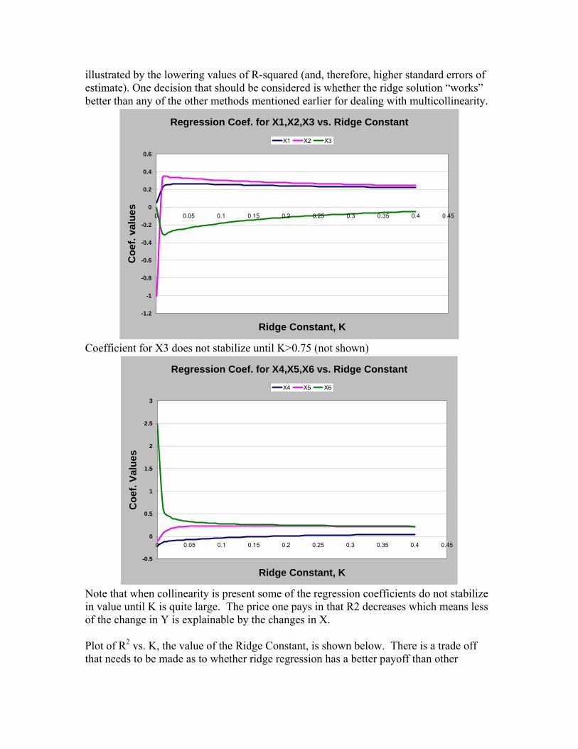
illustrated by the lowering values of R-squared (and, therefore, higher standard errors of estimate). One decision that should be considered is whether the ridge solution “works” better than any of the other methods mentioned earlier for dealing with multicollinearity.

Regression Coef. for X1,X2,X3 vs. Ridge Constant

-1.2

-1

-0.8

-0.6

-0.4

-0.2

0

0.2

0.4

0.6

0 0.05 0.1 0.15 0.2 0.25 0.3 0.35 0.4 0.45

Ridge Constant, K

Coe

f. va

lues

X1 X2 X3

Coefficient for X3 does not stabilize until K>0.75 (not shown)

Regression Coef. for X4,X5,X6 vs. Ridge Constant

-0.5

0

0.5

1

1.5

2

2.5

3

0 0.05 0.1 0.15 0.2 0.25 0.3 0.35 0.4 0.45

Ridge Constant, K

Coe

f. Va

lues

X4 X5 X6

Note that when collinearity is present some of the regression coefficients do not stabilize in value until K is quite large. The price one pays in that R2 decreases which means less of the change in Y is explainable by the changes in X.

Plot of R2 vs. K, the value of the Ridge Constant, is shown below. There is a trade off that needs to be made as to whether ridge regression has a better payoff than other

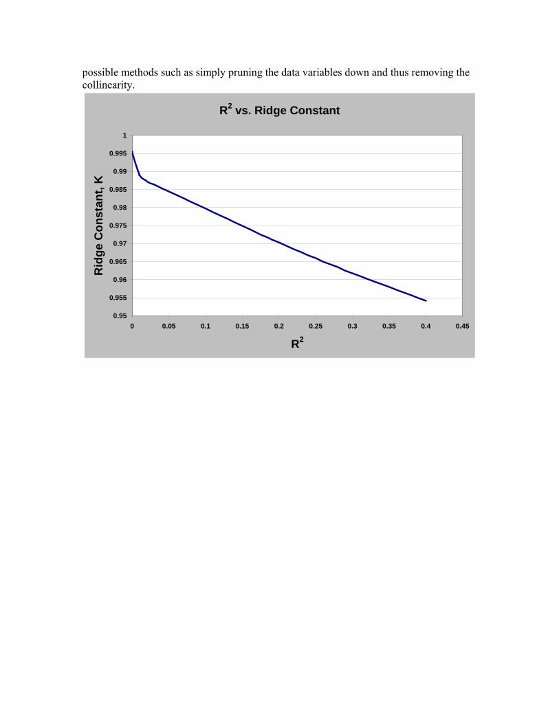
possible methods such as simply pruning the data variables down and thus removing the collinearity.

R2 vs. Ridge Constant

0.95

0.955

0.96

0.965

0.97

0.975

0.98

0.985

0.99

0.995

1

0 0.05 0.1 0.15 0.2 0.25 0.3 0.35 0.4 0.45

R2

Rid

ge C

onst

ant,

K

Generalized Orthogonal Solutions. This is a regression technique that selects linear combinations of the data vectors {X1, X2,…, Xk} that “correlate” most closely with the response Y and are orthogonal to one another. As opposed to selecting special levels of the factors X that will produce an orthogonal set of “causal” vectors one simply takes the data at hand and creates orthogonal causal vectors. This is useful when one already has data and has little prospect of getting any more data so you want the best fit to the data possible. This technique does just that as long as the input (causal or independent variable) vectors are not perfectly collinear.