Introduction to Regression Analysis

Dr. Devlina Chatterjee

11th August, 2017

What is regression analysis?

Regression analysis is a statistical technique for studying linear

relationships.

One dependent variable and one or more independent

variables, often called predictor variables.

Regression is being used more and more in “analytics”

research that affects many aspects of our daily lives, from how

much we pay for automobile insurance to which ads appear in

our social media.

Example of questions where regression

analysis is used

What is the effect of one more year of education on the

income of an individual?

What are the factors that indicate whether a particular

individual will get a job?

Can we predict how the price of a particular stock will

change in the next few weeks?

How will a particular policy such as change in taxes on

cigarettes affect the incidence of smoking in a state?

How long will a patient survive after being given a particular

treatment as compared to not being given that treatment?

Population vs. Sample

The research question may be – does more education lead to

more income?

We want to understand the relationship between two variables

(education and income) in the population

We do not have data for every person in the population

Look at data for a smaller sample drawn from the population

If the sample is “large enough” and drawn randomly from the

population, then we can make inferences about the population

from the relationships observed in the sample

The reason we can draw inferences is because of two

fundamental theorems in probability:

“Law of Large Numbers” and “Central Limit Theorem”.

Sampling Distributions

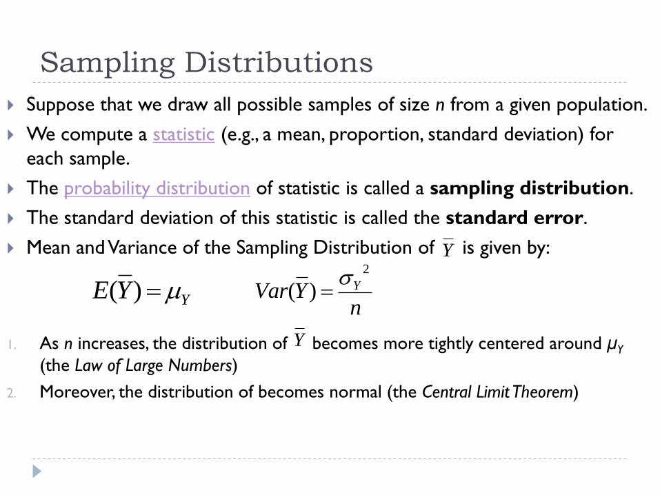
Suppose that we draw all possible samples of size n from a given population.

We compute a statistic (e.g., a mean, proportion, standard deviation) for

each sample.

The probability distribution of statistic is called a sampling distribution.

The standard deviation of this statistic is called the standard error.

Mean and Variance of the Sampling Distribution of is given by:

1. As n increases, the distribution of becomes more tightly centered around μY

(the Law of Large Numbers)

2. Moreover, the distribution of becomes normal (the Central Limit Theorem)

YYE )(n

YVar Y

2

)(

Y

Y

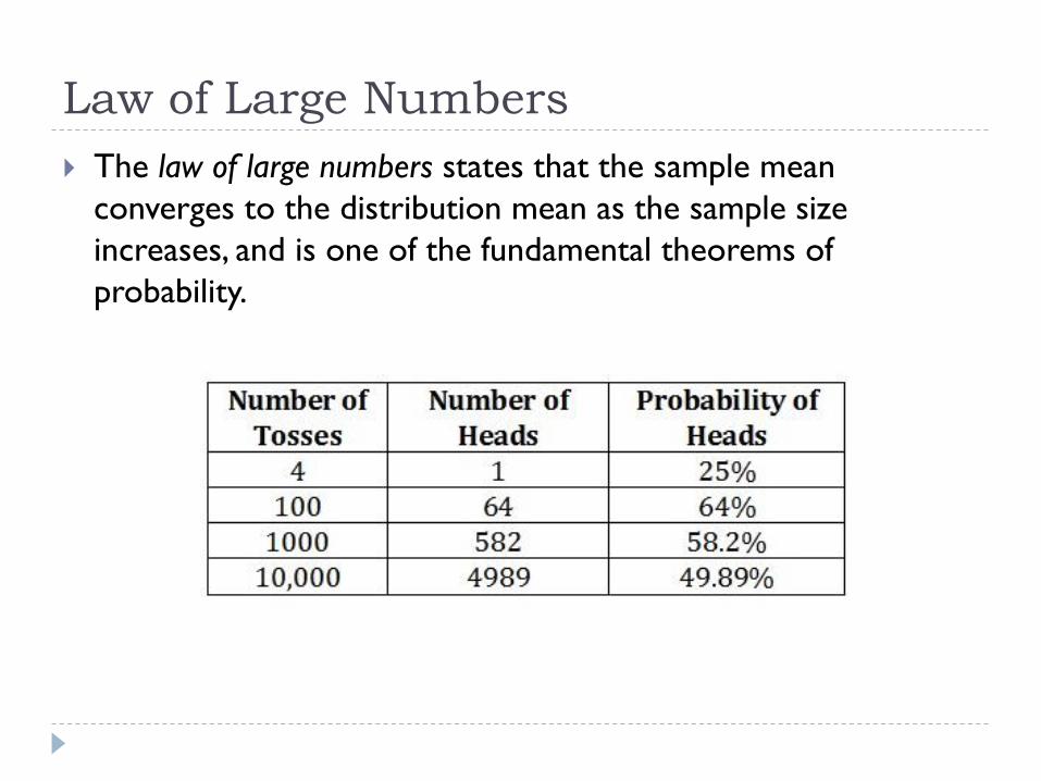
Law of Large Numbers

The law of large numbers states that the sample mean

converges to the distribution mean as the sample size

increases, and is one of the fundamental theorems of

probability.

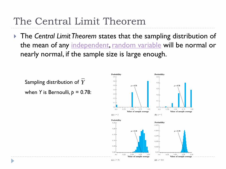
The Central Limit Theorem

The Central Limit Theorem states that the sampling distribution of

the mean of any independent, random variable will be normal or

nearly normal, if the sample size is large enough.

Sampling distribution of

when Y is Bernoulli, p = 0.78:

Y

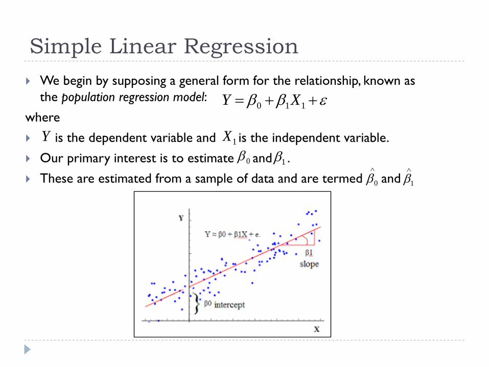
Simple Linear Regression

We begin by supposing a general form for the relationship, known as

the population regression model:

where

is the dependent variable and is the independent variable.

Our primary interest is to estimate and .

These are estimated from a sample of data and are termed and

110 XY

Y 1X

0 1

0

1

Reasons for doing Regression

Determining whether there is evidence that an explanatory variable

belongs in a regression model (Statistical significance of a variable)

Estimating the effect of an explanatory variable on the dependent variable

(Effect Size – magnitude of the coefficient )

Measuring the explanatory power of a model (R2)

Making individual predictions for individuals not in the original sample

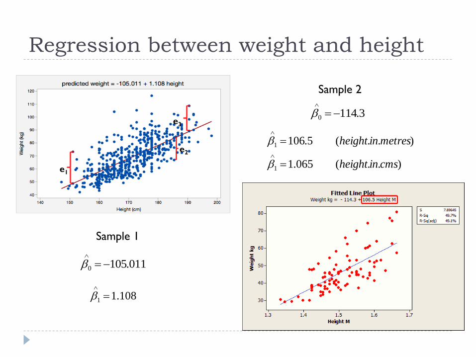
Regression between weight and height

e1

e2

e3

Sample 1

Sample 2

011.1050

108.11

3.1140

)..(065.1

)..(5.106

1

1

cmsinheight

metresinheight

The idea of statistical significance

Someone may look at the regression results from Sample 1 and Sample 2

and see that the results are slightly different.

How much confidence can we have in the values of and estimated

from our first sample?

We need to test the hypothesis that there is indeed a non-zero correlation

between Y and X

Which translates to testing the null hypotheses: and

0

1

00

01

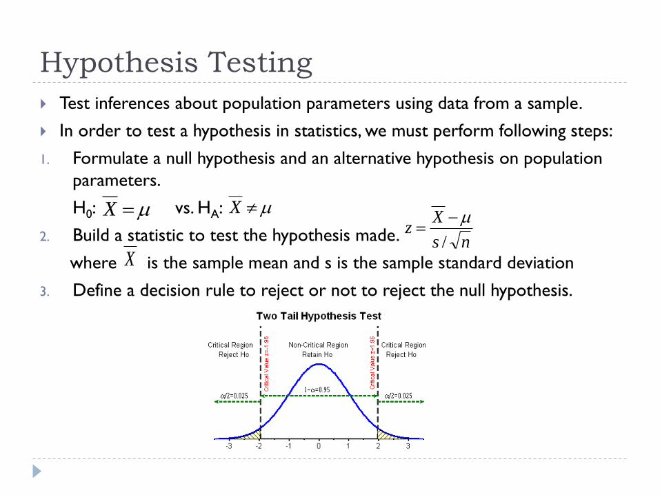
Hypothesis Testing

Test inferences about population parameters using data from a sample.

In order to test a hypothesis in statistics, we must perform following steps:

1. Formulate a null hypothesis and an alternative hypothesis on population

parameters.

H0: vs. HA:

2. Build a statistic to test the hypothesis made.

where is the sample mean and s is the sample standard deviation

3. Define a decision rule to reject or not to reject the null hypothesis.

ns

Xz

/

X X

X

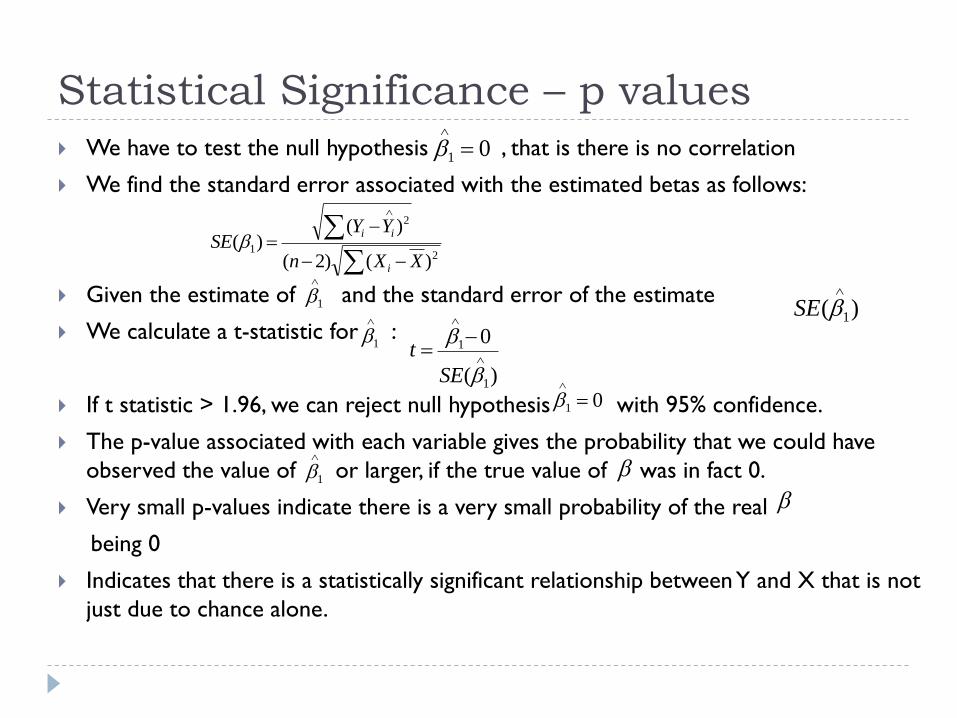
Statistical Significance – p values

We have to test the null hypothesis , that is there is no correlation

We find the standard error associated with the estimated betas as follows:

Given the estimate of and the standard error of the estimate

We calculate a t-statistic for :

If t statistic > 1.96, we can reject null hypothesis with 95% confidence.

The p-value associated with each variable gives the probability that we could have

observed the value of or larger, if the true value of was in fact 0.

Very small p-values indicate there is a very small probability of the real

being 0

Indicates that there is a statistically significant relationship between Y and X that is not

just due to chance alone.

2

2

1

)()2(

)()(

XXn

YYSE

i

ii

01

1 )( 1

SE

1

)(

0

1

1

SE

t

01

1

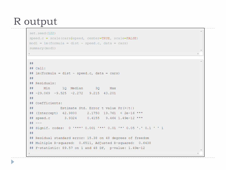
R output

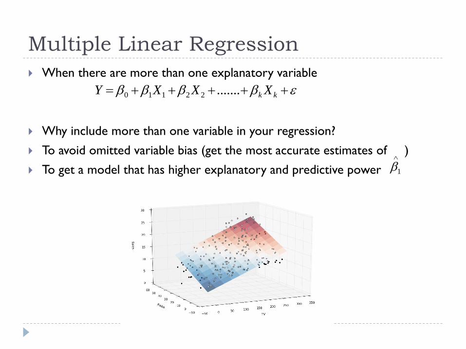
Multiple Linear Regression

When there are more than one explanatory variable

Why include more than one variable in your regression?

To avoid omitted variable bias (get the most accurate estimates of )

To get a model that has higher explanatory and predictive power

kk XXXY .......22110

1

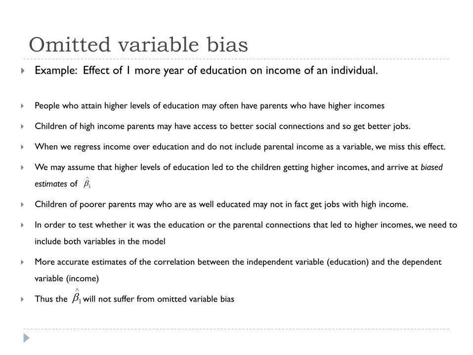
Omitted variable bias Example: Effect of 1 more year of education on income of an individual.

People who attain higher levels of education may often have parents who have higher incomes

Children of high income parents may have access to better social connections and so get better jobs.

When we regress income over education and do not include parental income as a variable, we miss this effect.

We may assume that higher levels of education led to the children getting higher incomes, and arrive at biased

estimates of

Children of poorer parents may who are as well educated may not in fact get jobs with high income.

In order to test whether it was the education or the parental connections that led to higher incomes, we need to

include both variables in the model

More accurate estimates of the correlation between the independent variable (education) and the dependent

variable (income)

Thus the will not suffer from omitted variable bias

1

1

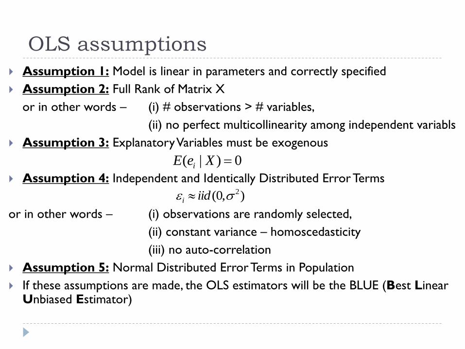
OLS assumptions

Assumption 1: Model is linear in parameters and correctly specified

Assumption 2: Full Rank of Matrix X

or in other words – (i) # observations > # variables,

(ii) no perfect multicollinearity among independent variabls

Assumption 3: Explanatory Variables must be exogenous

Assumption 4: Independent and Identically Distributed Error Terms

or in other words – (i) observations are randomly selected,

(ii) constant variance – homoscedasticity

(iii) no auto-correlation

Assumption 5: Normal Distributed Error Terms in Population

If these assumptions are made, the OLS estimators will be the BLUE (Best Linear Unbiased Estimator)

0)|( XeE i

),0( 2 iidi

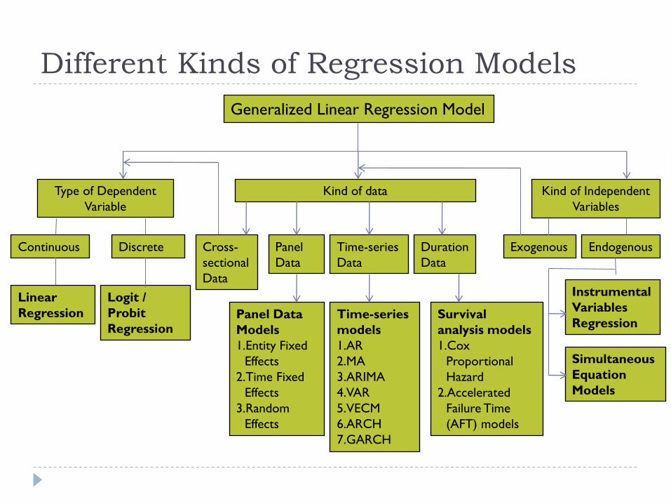
Different Kinds of Regression Models

Generalized Linear Regression Model

Type of Dependent

Variable

Kind of data

DiscreteContinuous Cross-

sectional

Data

Time-series

Data

Duration

Data

Linear

Regression

Logit /

Probit

RegressionTime-series

models

1.AR

2.MA

3.ARIMA

4.VAR

5.VECM

6.ARCH

7.GARCH

Panel

Data

Panel Data

Models

1.Entity Fixed

Effects

2.Time Fixed

Effects

3.Random

Effects

Survival

analysis models

1.Cox

Proportional

Hazard

2.Accelerated

Failure Time

(AFT) models

Kind of Independent

Variables

EndogenousExogenous

Instrumental

Variables

Regression

Simultaneous

Equation

Models

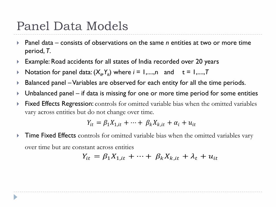
Panel Data Models

Panel data – consists of observations on the same n entities at two or more time

period, T.

Example: Road accidents for all states of India recorded over 20 years

Notation for panel data: (Xit, Yit) where i = 1,....,n and t = 1,....,T

Balanced panel –Variables are observed for each entity for all the time periods.

Unbalanced panel – if data is missing for one or more time period for some entities

Fixed Effects Regression: controls for omitted variable bias when the omitted variables

vary across entities but do not change over time.

Time Fixed Effects controls for omitted variable bias when the omitted variables vary

over time but are constant across entities

𝑌𝑖𝑡 = 𝛽1𝑋1,𝑖𝑡 + ⋯+ 𝛽𝑘𝑋𝑘 ,𝑖𝑡 + 𝛼𝑖 + 𝑢𝑖𝑡

𝑌𝑖𝑡 = 𝛽1𝑋1,𝑖𝑡 + ⋯+ 𝛽𝑘𝑋𝑘 ,𝑖𝑡 + 𝜆𝑡 + 𝑢𝑖𝑡

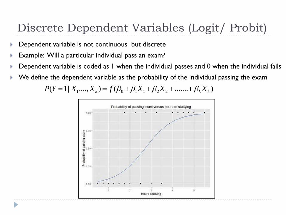
Discrete Dependent Variables (Logit/ Probit)

Dependent variable is not continuous but discrete

Example: Will a particular individual pass an exam?

Dependent variable is coded as 1 when the individual passes and 0 when the individual fails

We define the dependent variable as the probability of the individual passing the exam

).......(),...,|1( 221101 kkk XXXfXXYP

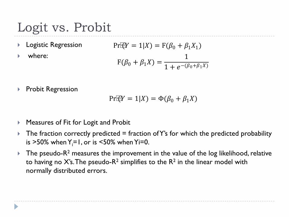
Logit vs. Probit

Logistic Regression

where:

Probit Regression

Measures of Fit for Logit and Probit

The fraction correctly predicted = fraction of Y’s for which the predicted probability

is >50% when Yi=1, or is <50% when Yi=0.

The pseudo-R2 measures the improvement in the value of the log likelihood, relative

to having no X’s. The pseudo-R2 simplifies to the R2 in the linear model with

normally distributed errors.

Pr(𝑌 = 1|𝑋) = F(𝛽0 + 𝛽1𝑋1)

F(𝛽0 + 𝛽1𝑋) =1

1 + 𝑒−(𝛽0+𝛽1𝑋)

Pr(𝑌 = 1|𝑋) = Φ(𝛽0 + 𝛽1𝑋)

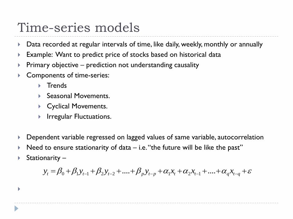
Time-series models Data recorded at regular intervals of time, like daily, weekly, monthly or annually

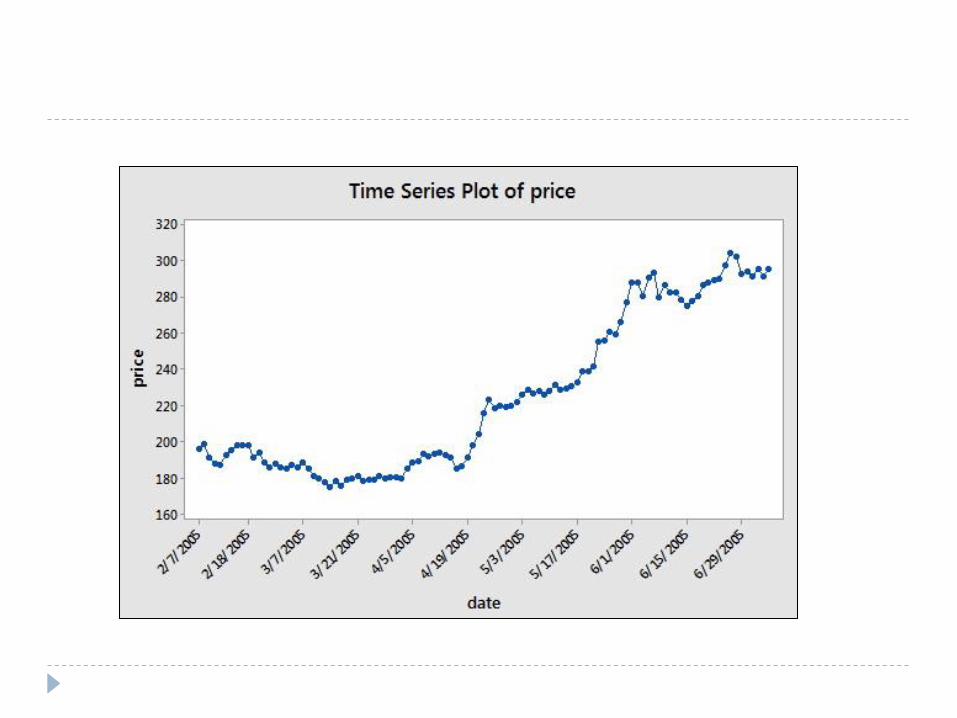
Example: Want to predict price of stocks based on historical data

Primary objective – prediction not understanding causality

Components of time-series:

Trends

Seasonal Movements.

Cyclical Movements.

Irregular Fluctuations.

Dependent variable regressed on lagged values of same variable, autocorrelation

Need to ensure stationarity of data – i.e. “the future will be like the past”

Stationarity –

qtqttptpttt xxxyyyy ........ 12122110

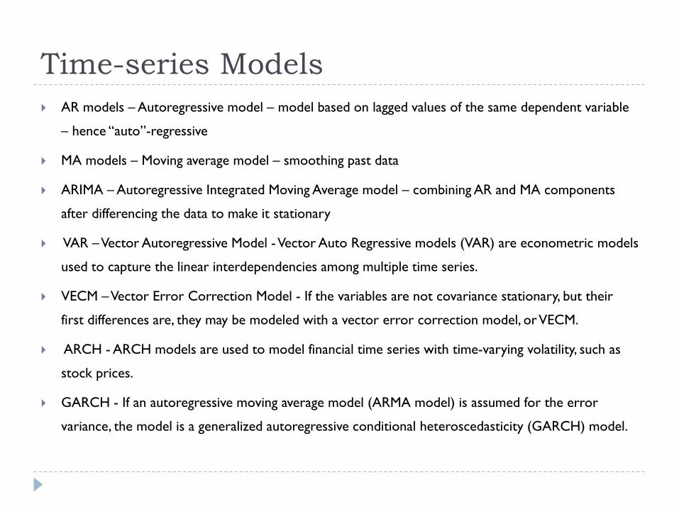
Time-series Models

AR models – Autoregressive model – model based on lagged values of the same dependent variable

– hence “auto”-regressive

MA models – Moving average model – smoothing past data

ARIMA – Autoregressive Integrated Moving Average model – combining AR and MA components

after differencing the data to make it stationary

VAR –Vector Autoregressive Model -Vector Auto Regressive models (VAR) are econometric models

used to capture the linear interdependencies among multiple time series.

VECM –Vector Error Correction Model - If the variables are not covariance stationary, but their

first differences are, they may be modeled with a vector error correction model, or VECM.

ARCH - ARCH models are used to model financial time series with time-varying volatility, such as

stock prices.

GARCH - If an autoregressive moving average model (ARMA model) is assumed for the error

variance, the model is a generalized autoregressive conditional heteroscedasticity (GARCH) model.