Embed Size (px)
Citation preview
CVE 475 Statistical Techniques in Hydrology 1/80
Simple Linear Regression and Correlation
In this chapter, you learn:How to use regression analysis to predict the value of a dependent variable based on an independent variableThe meaning of the regression coefficients b0 and b1
How to evaluate the assumptions of regression analysis and know what to do if the assumptions are violatedTo make inferences about the slope and correlation coefficientTo estimate mean values and predict individual values
CVE 475 Statistical Techniques in Hydrology 2/80
Correlation vs. Regression
A scatter diagram can be used to show the relationship between two variables
Correlation analysis is used to measure strength of the association (linear relationship) between two variables
Correlation is only concerned with strength of the relationship
No causal effect is implied with correlation
CVE 475 Statistical Techniques in Hydrology 3/80
Introduction to Regression Analysis
Regression analysis is used to:Predict the value of a dependent variable based on the value of at least one independent variable
Explain the impact of changes in an independent variable on the dependent variable
Dependent variable: the variable we wish to predictor explain (i.e. runoff)
Independent variable: the variable used to explain the dependent variable (i.e. rainfall)
CVE 475 Statistical Techniques in Hydrology 4/80
Simple Linear Regression Model
Only one independent variable, X
Relationship between X and Y is described by a linear function
Changes in Y are assumed to be caused by changes in X
CVE 475 Statistical Techniques in Hydrology 5/80
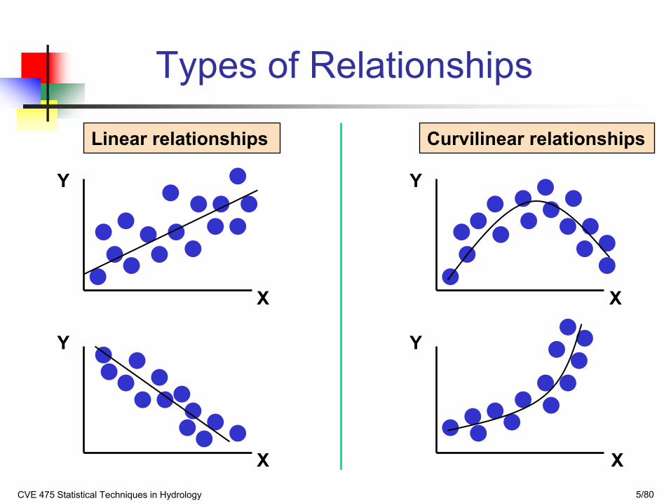
Types of Relationships
Y
X
Y
X
Y
Y
X
X
Linear relationships Curvilinear relationships
CVE 475 Statistical Techniques in Hydrology 6/80
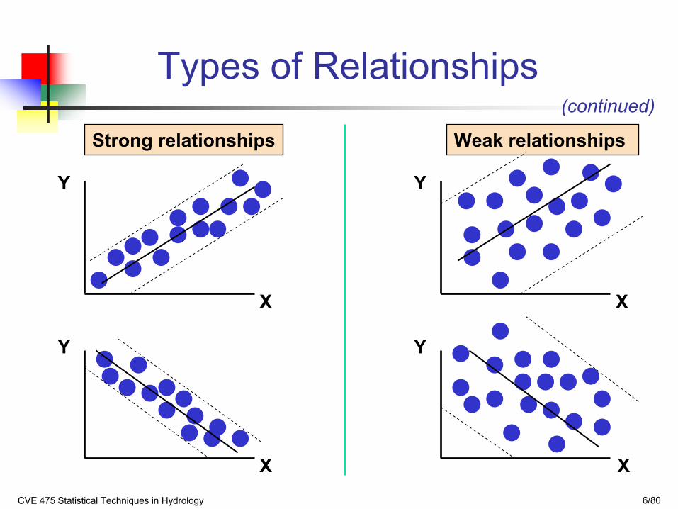
Types of Relationships
Y
X
Y
X
Y
Y
X
X
Strong relationships Weak relationships
(continued)
CVE 475 Statistical Techniques in Hydrology 7/80
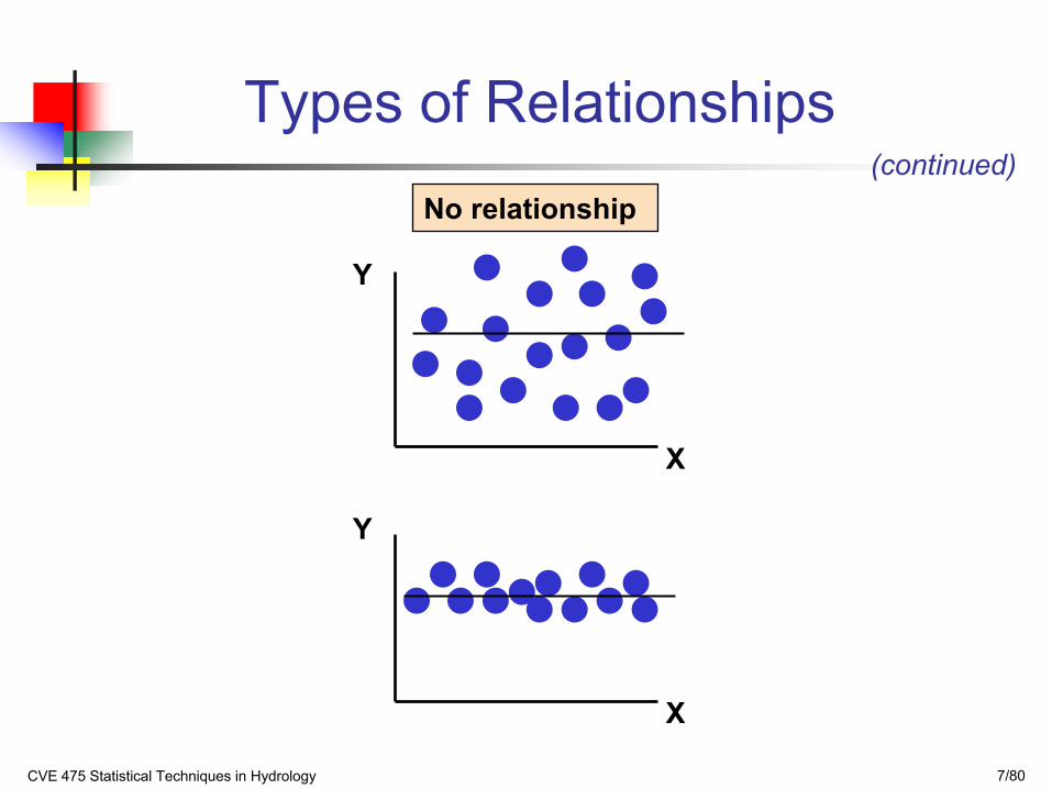
Types of Relationships
Y
X
Y
X
No relationship(continued)
CVE 475 Statistical Techniques in Hydrology 8/80
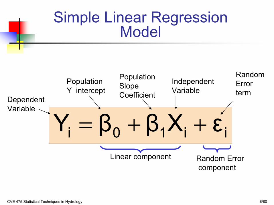
ii10i εXββY ++=Linear component
Simple Linear Regression Model
Population Y intercept
Population SlopeCoefficient
Random Error term
Dependent Variable
Independent Variable
Random Errorcomponent
CVE 475 Statistical Techniques in Hydrology 9/80
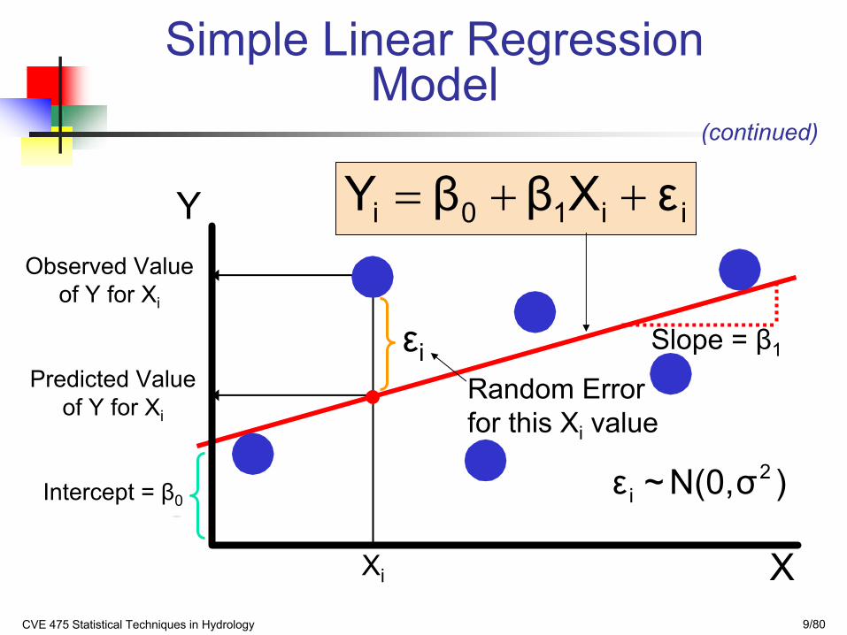
(continued)
Random Error for this Xi value
Y
X
Observed Value of Y for Xi
Predicted Value of Y for Xi
ii10i εXββY ++=
Xi
Slope = β1
Intercept = β0
εi
Simple Linear Regression Model
)σN(0,~ε 2i
CVE 475 Statistical Techniques in Hydrology 10/80
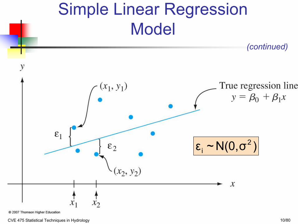
Simple Linear Regression Model
)σN(0,~ε 2i
(continued)
CVE 475 Statistical Techniques in Hydrology 11/80
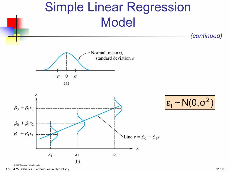
Simple Linear Regression Model
(continued)
)σN(0,~ε 2i
CVE 475 Statistical Techniques in Hydrology 12/80
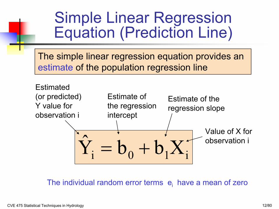
i10i XbbY +=
The simple linear regression equation provides an estimate of the population regression line
Simple Linear Regression Equation (Prediction Line)
Estimate of the regression intercept
Estimate of the regression slope
Estimated (or predicted) Y value for observation i
Value of X for observation i
The individual random error terms ei have a mean of zero
CVE 475 Statistical Techniques in Hydrology 13/80
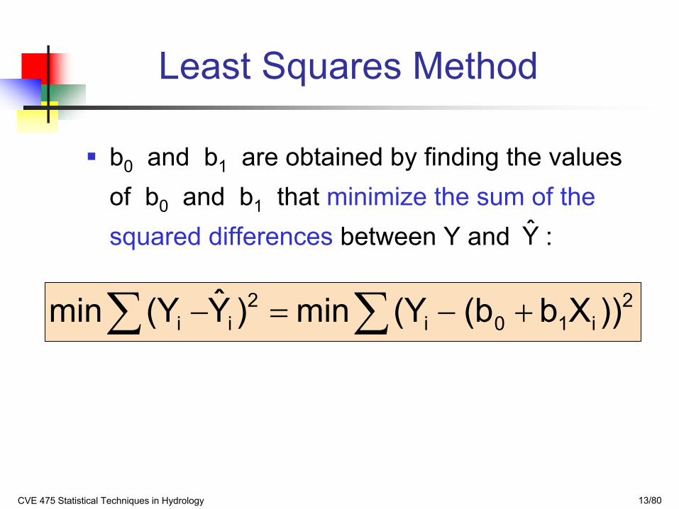
Least Squares Method
b0 and b1 are obtained by finding the values of b0 and b1 that minimize the sum of the squared differences between Y and :
2i10i
2ii ))Xb(b(Ymin)Y(Ymin +−=− ∑∑
Y
CVE 475 Statistical Techniques in Hydrology 14/80
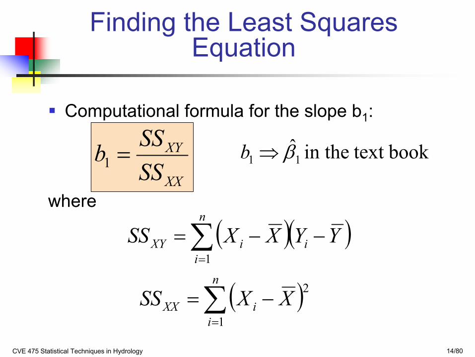
Finding the Least Squares Equation
Computational formula for the slope b1:
whereXX
XY
SSSSb =1
( )( )
( )∑
∑
=
=
−=
−−=
n
iiXX
i
n
iiXY
XXSS
YYXXSS
1
2
1
book text in the11 β⇒b
CVE 475 Statistical Techniques in Hydrology 15/80
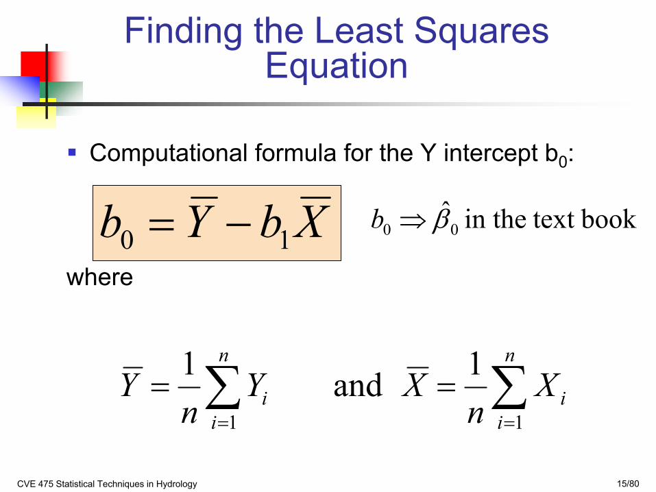
Finding the Least Squares Equation
Computational formula for the Y intercept b0:
where
XbYb 10 −=
∑∑==
==n
ii
n
ii X
nXY
nY
11
1and1
book text in theˆ00 β⇒b
CVE 475 Statistical Techniques in Hydrology 16/80
Finding the Least Squares Equation
The coefficients b0 and b1 , and other regression results in this chapter, will be found using Excel
CVE 475 Statistical Techniques in Hydrology 17/80
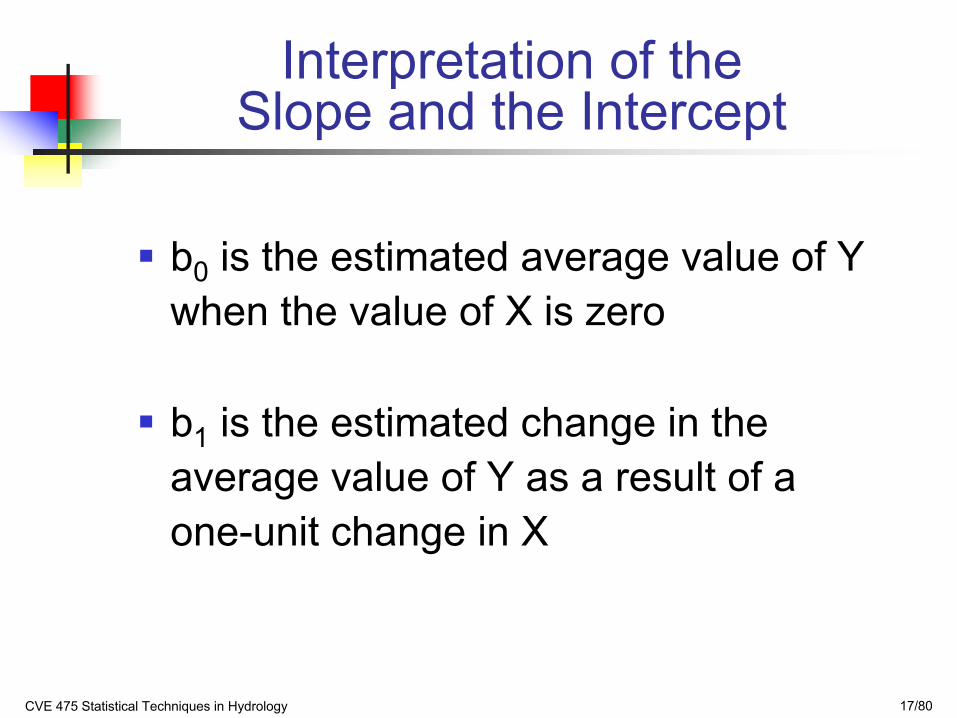
b0 is the estimated average value of Y when the value of X is zero
b1 is the estimated change in the average value of Y as a result of a one-unit change in X
Interpretation of the Slope and the Intercept
CVE 475 Statistical Techniques in Hydrology 18/80
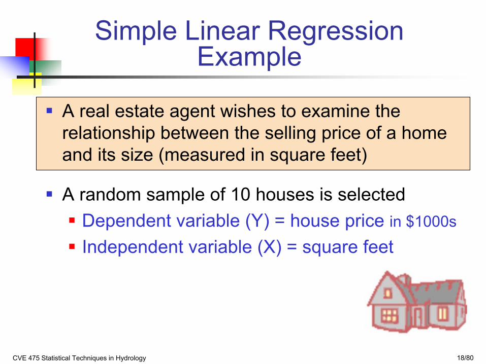
Simple Linear Regression Example
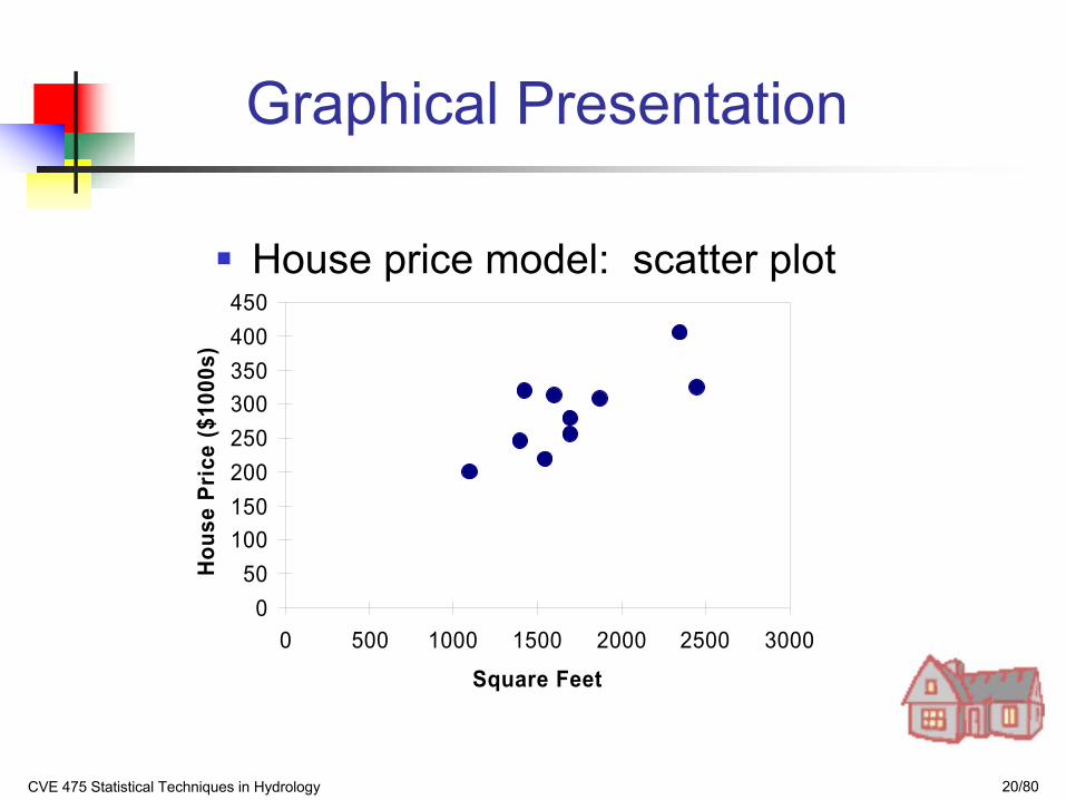
A real estate agent wishes to examine the relationship between the selling price of a home and its size (measured in square feet)
A random sample of 10 houses is selectedDependent variable (Y) = house price in $1000s
Independent variable (X) = square feet
CVE 475 Statistical Techniques in Hydrology 19/80
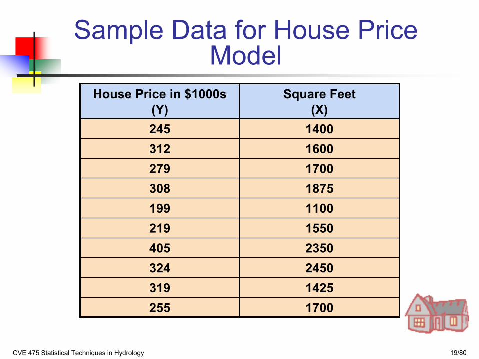
Sample Data for House Price Model
1700255142531924503242350405155021911001991875308170027916003121400245
Square Feet (X)
House Price in $1000s(Y)
CVE 475 Statistical Techniques in Hydrology 20/80
050
100150200250300350400450
0 500 1000 1500 2000 2500 3000
Square Feet
Hou
se P
rice
($10
00s)
Graphical Presentation
House price model: scatter plot
CVE 475 Statistical Techniques in Hydrology 21/80
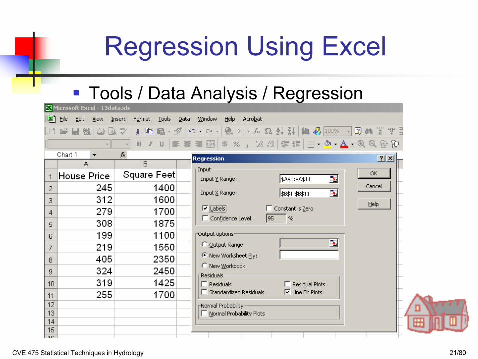
Regression Using ExcelTools / Data Analysis / Regression
CVE 475 Statistical Techniques in Hydrology 22/80
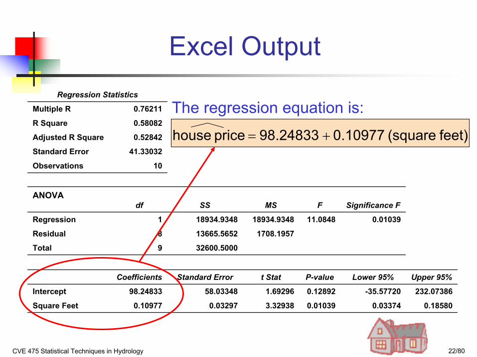
Excel Output
0.185800.033740.010393.329380.032970.10977Square Feet
232.07386-35.577200.128921.6929658.0334898.24833Intercept
Upper 95%Lower 95%P-valuet StatStandard ErrorCoefficients
32600.50009Total
1708.195713665.56528Residual
0.0103911.084818934.934818934.93481Regression
Significance FFMSSSdfANOVA
10Observations
41.33032Standard Error
0.52842Adjusted R Square
0.58082R Square
0.76211Multiple R
Regression Statistics
The regression equation is:
feet) (square 0.10977 98.24833 price house +=
CVE 475 Statistical Techniques in Hydrology 23/80
050
100150200250300350400450
0 500 1000 1500 2000 2500 3000
Square Feet
Hou
se P
rice
($10
00s)
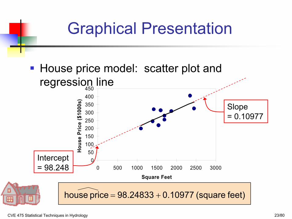
Graphical Presentation
House price model: scatter plot and regression line
feet) (square 0.10977 98.24833 price house +=
Slope = 0.10977
Intercept = 98.248
CVE 475 Statistical Techniques in Hydrology 24/80
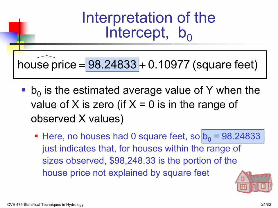
Interpretation of the Intercept, b0
b0 is the estimated average value of Y when the value of X is zero (if X = 0 is in the range of observed X values)
Here, no houses had 0 square feet, so b0 = 98.24833 just indicates that, for houses within the range of sizes observed, $98,248.33 is the portion of the house price not explained by square feet
feet) (square 0.10977 98.24833 price house +=
CVE 475 Statistical Techniques in Hydrology 25/80
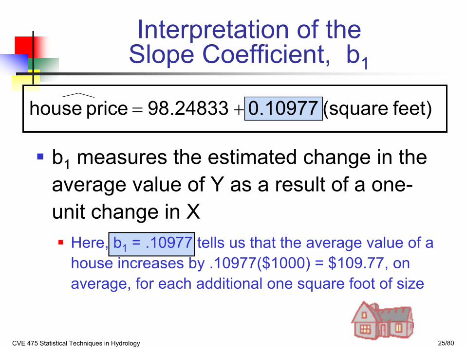
Interpretation of the Slope Coefficient, b1
b1 measures the estimated change in the average value of Y as a result of a one-unit change in X
Here, b1 = .10977 tells us that the average value of a house increases by .10977($1000) = $109.77, on average, for each additional one square foot of size
feet) (square 0.10977 98.24833 price house +=
CVE 475 Statistical Techniques in Hydrology 26/80
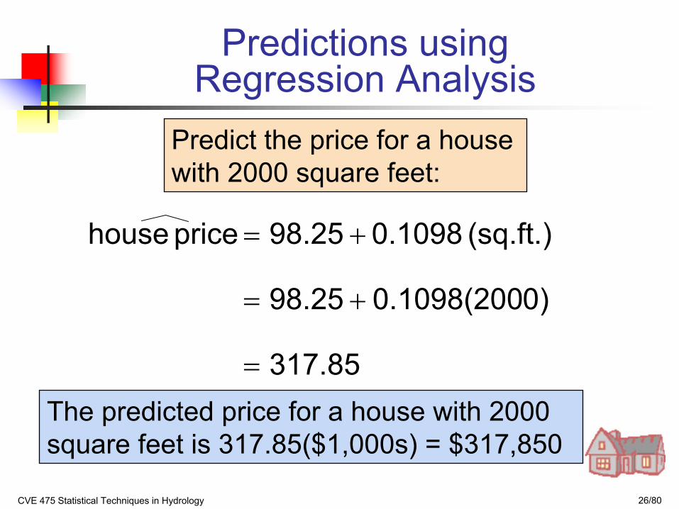
317.85
0)0.1098(200 98.25
(sq.ft.) 0.1098 98.25 price house
=
+=
+=
Predict the price for a house with 2000 square feet:
The predicted price for a house with 2000 square feet is 317.85($1,000s) = $317,850
Predictions using Regression Analysis
CVE 475 Statistical Techniques in Hydrology 27/80
050
100150200250300350400450
0 500 1000 1500 2000 2500 3000
Square Feet
Hou
se P
rice
($10
00s)
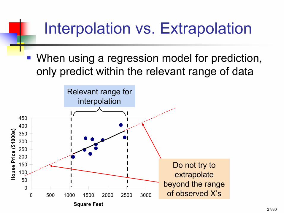
Interpolation vs. Extrapolation
When using a regression model for prediction, only predict within the relevant range of data
Relevant range for interpolation
Do not try to extrapolate
beyond the range of observed X’s
CVE 475 Statistical Techniques in Hydrology 28/80
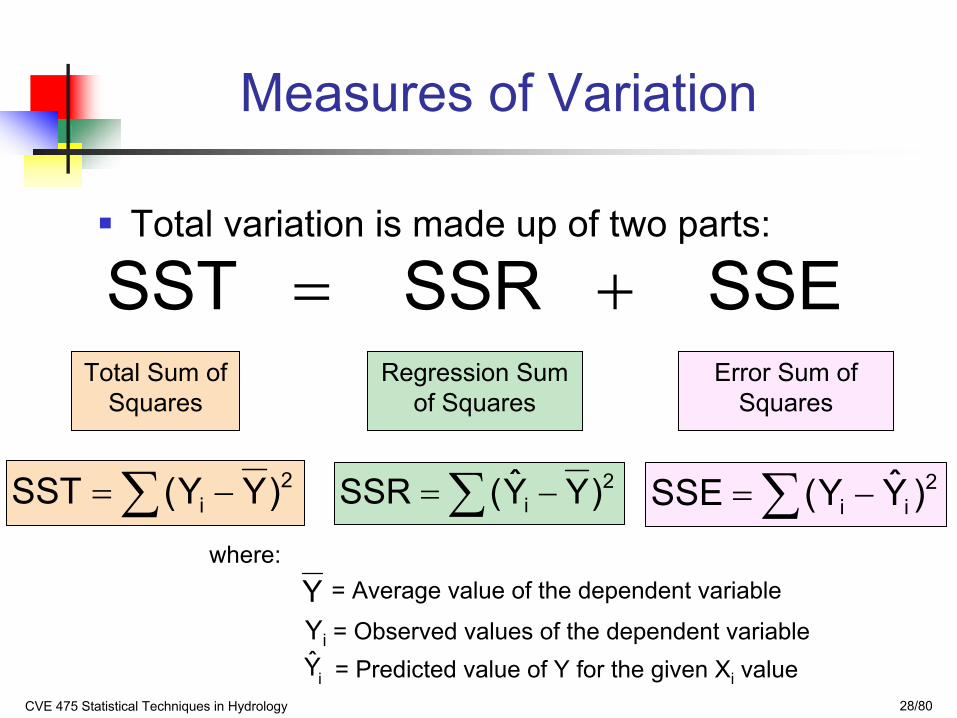
Measures of Variation
Total variation is made up of two parts:
SSE SSR SST +=Total Sum of
SquaresRegression Sum
of SquaresError Sum of
Squares
∑ −= 2i )YY(SST ∑ −= 2
ii )YY(SSE∑ −= 2i )YY(SSR
where:= Average value of the dependent variable
Yi = Observed values of the dependent variable
i = Predicted value of Y for the given Xi valueY
Y
CVE 475 Statistical Techniques in Hydrology 29/80
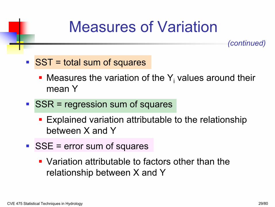
SST = total sum of squares
Measures the variation of the Yi values around their mean Y
SSR = regression sum of squares
Explained variation attributable to the relationship between X and Y
SSE = error sum of squares
Variation attributable to factors other than the relationship between X and Y
(continued)
Measures of Variation
CVE 475 Statistical Techniques in Hydrology 30/80
(continued)
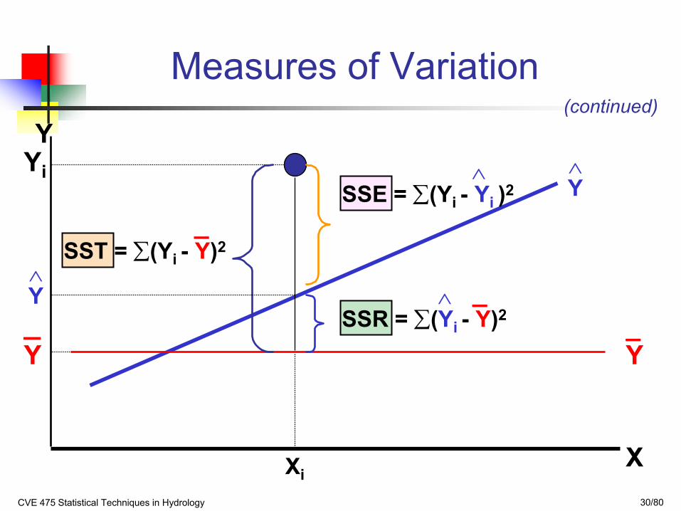
Xi
Y
X
Yi
SST = ∑(Yi - Y)2
SSE = ∑(Yi - Yi )2∧
SSR = ∑(Yi - Y)2∧
__
_Y∧
Y
Y_Y∧
Measures of Variation
CVE 475 Statistical Techniques in Hydrology 31/80
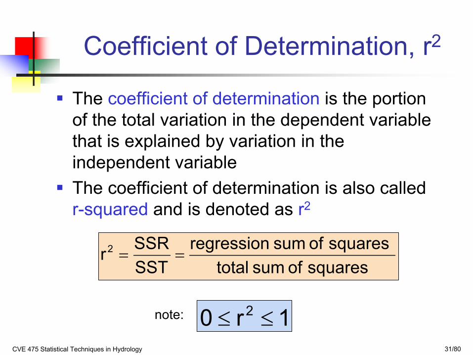
The coefficient of determination is the portion of the total variation in the dependent variable that is explained by variation in the independent variableThe coefficient of determination is also called r-squared and is denoted as r2
Coefficient of Determination, r2
1r0 2 ≤≤note:
squares of sum total squares of sum regression
SSTSSRr2 ==
CVE 475 Statistical Techniques in Hydrology 32/80
r2 = 1
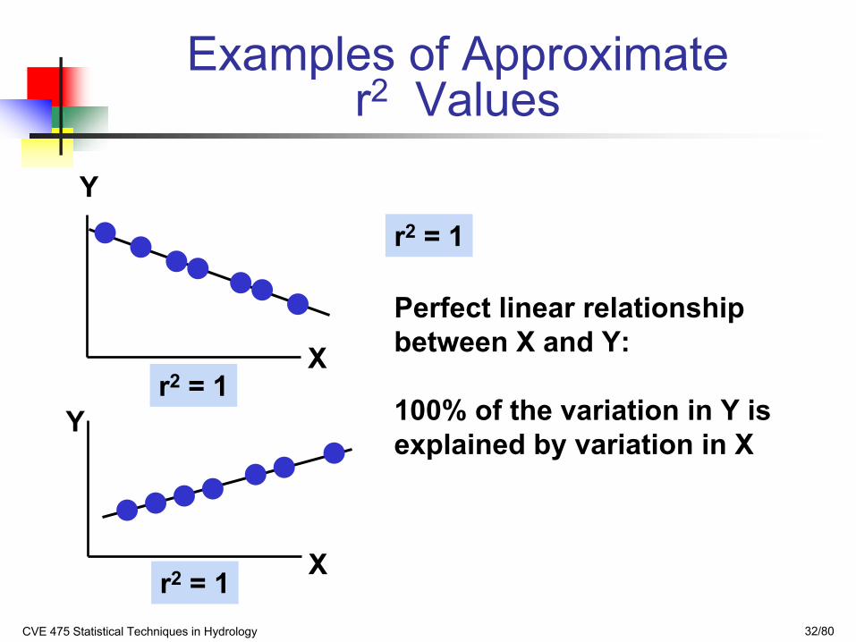
Examples of Approximate r2 Values
Y
X
Y
X
r2 = 1
r2 = 1
Perfect linear relationship between X and Y:
100% of the variation in Y is explained by variation in X
CVE 475 Statistical Techniques in Hydrology 33/80
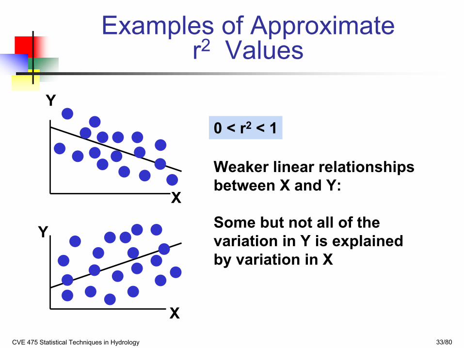
Examples of Approximate r2 Values
Y
X
Y
X
0 < r2 < 1
Weaker linear relationships between X and Y:
Some but not all of the variation in Y is explained by variation in X
CVE 475 Statistical Techniques in Hydrology 34/80
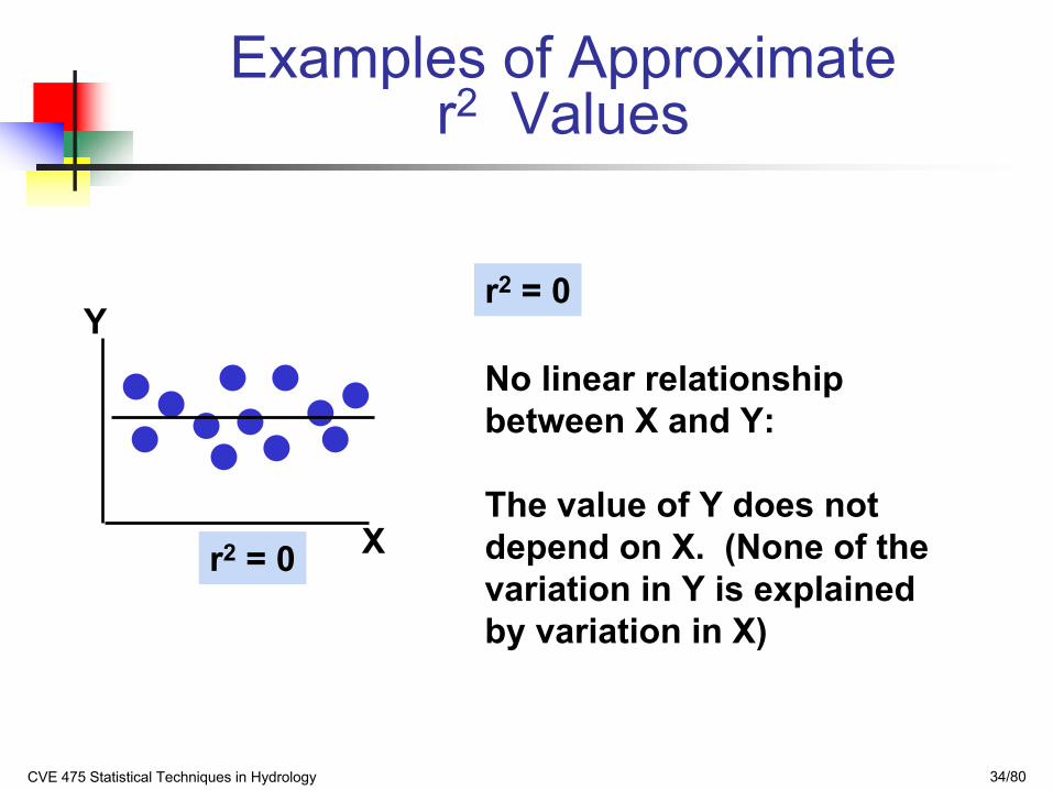
Examples of Approximate r2 Values
r2 = 0
No linear relationship between X and Y:
The value of Y does not depend on X. (None of the variation in Y is explained by variation in X)
Y
Xr2 = 0
CVE 475 Statistical Techniques in Hydrology 35/80
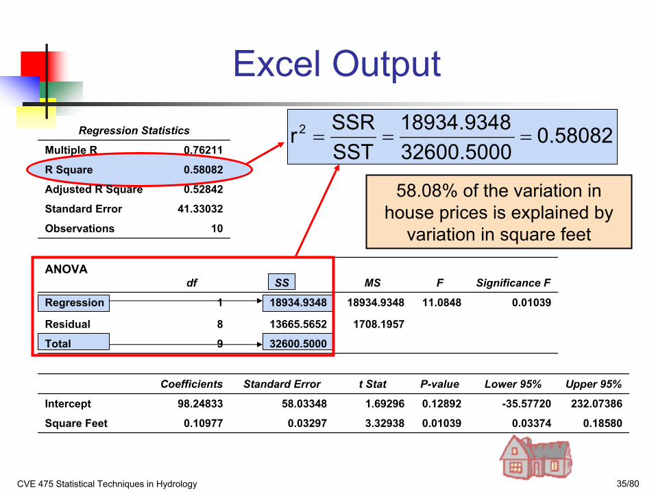
Excel Output
0.185800.033740.010393.329380.032970.10977Square Feet
232.07386-35.577200.128921.6929658.0334898.24833Intercept
Upper 95%Lower 95%P-valuet StatStandard ErrorCoefficients
32600.50009Total
1708.195713665.56528Residual
0.0103911.084818934.934818934.93481Regression
Significance FFMSSSdfANOVA
10Observations
41.33032Standard Error
0.52842Adjusted R Square
0.58082R Square
0.76211Multiple R
Regression Statistics
58.08% of the variation in house prices is explained by
variation in square feet
0.5808232600.500018934.9348
SSTSSRr2 ===
CVE 475 Statistical Techniques in Hydrology 36/80
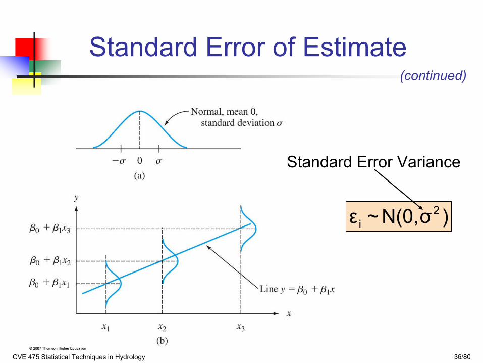
Standard Error of Estimate(continued)
)σN(0,~ε 2i
Standard Error Variance
CVE 475 Statistical Techniques in Hydrology 37/80
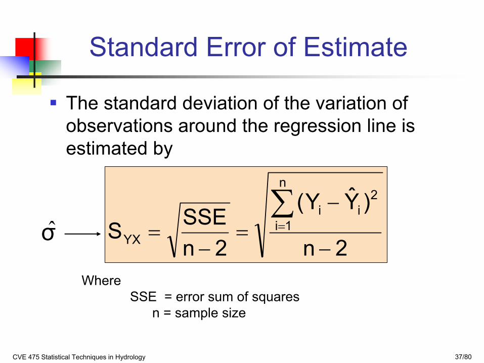
Standard Error of Estimate
The standard deviation of the variation of observations around the regression line is estimated by
2n
)YY(
2nSSES
n
1i
2ii
YX −
−=
−=
∑=
WhereSSE = error sum of squares
n = sample size
σ
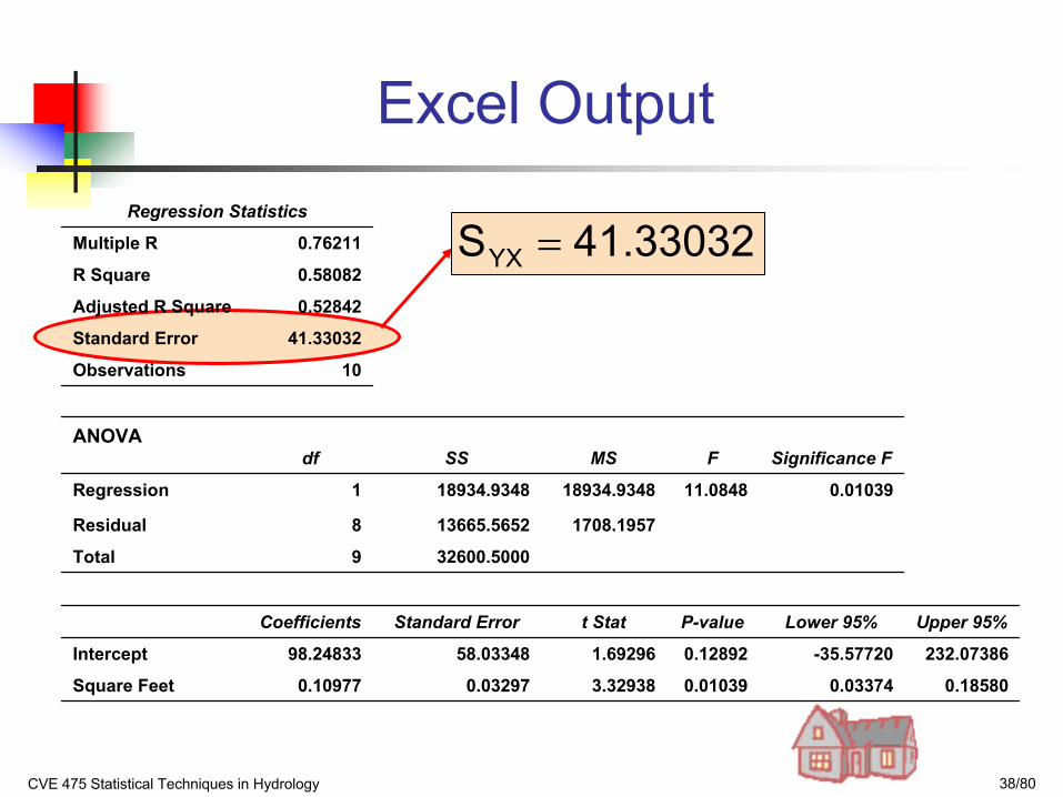
CVE 475 Statistical Techniques in Hydrology 38/80
Excel Output
0.185800.033740.010393.329380.032970.10977Square Feet
232.07386-35.577200.128921.6929658.0334898.24833Intercept
Upper 95%Lower 95%P-valuet StatStandard ErrorCoefficients
32600.50009Total
1708.195713665.56528Residual
0.0103911.084818934.934818934.93481Regression
Significance FFMSSSdfANOVA
10Observations
41.33032Standard Error
0.52842Adjusted R Square
0.58082R Square
0.76211Multiple R
Regression Statistics
41.33032SYX =
CVE 475 Statistical Techniques in Hydrology 39/80
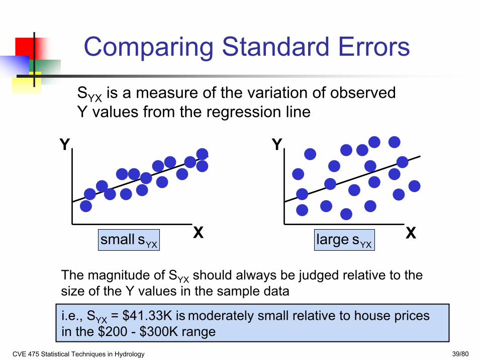
Comparing Standard Errors
YY
X XYXs small YXs large
SYX is a measure of the variation of observed Y values from the regression line
The magnitude of SYX should always be judged relative to the size of the Y values in the sample data
i.e., SYX = $41.33K is moderately small relative to house prices in the $200 - $300K range
CVE 475 Statistical Techniques in Hydrology 40/80
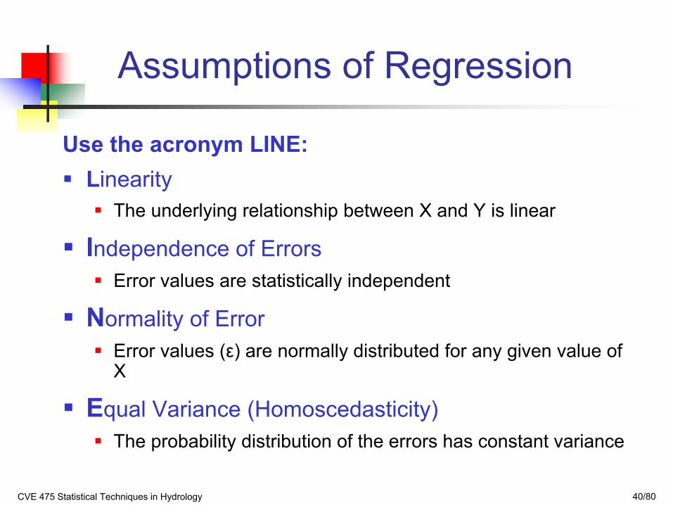
Assumptions of Regression
Use the acronym LINE:Linearity
The underlying relationship between X and Y is linear
Independence of ErrorsError values are statistically independent
Normality of ErrorError values (ε) are normally distributed for any given value of X
Equal Variance (Homoscedasticity)The probability distribution of the errors has constant variance
CVE 475 Statistical Techniques in Hydrology 41/80
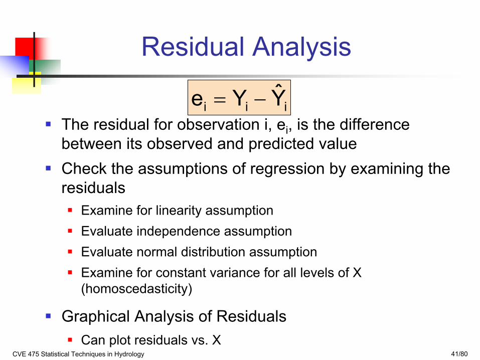
Residual Analysis
The residual for observation i, ei, is the difference between its observed and predicted valueCheck the assumptions of regression by examining the residuals
Examine for linearity assumptionEvaluate independence assumption Evaluate normal distribution assumption Examine for constant variance for all levels of X (homoscedasticity)
Graphical Analysis of ResidualsCan plot residuals vs. X
iii YYe −=
CVE 475 Statistical Techniques in Hydrology 42/80
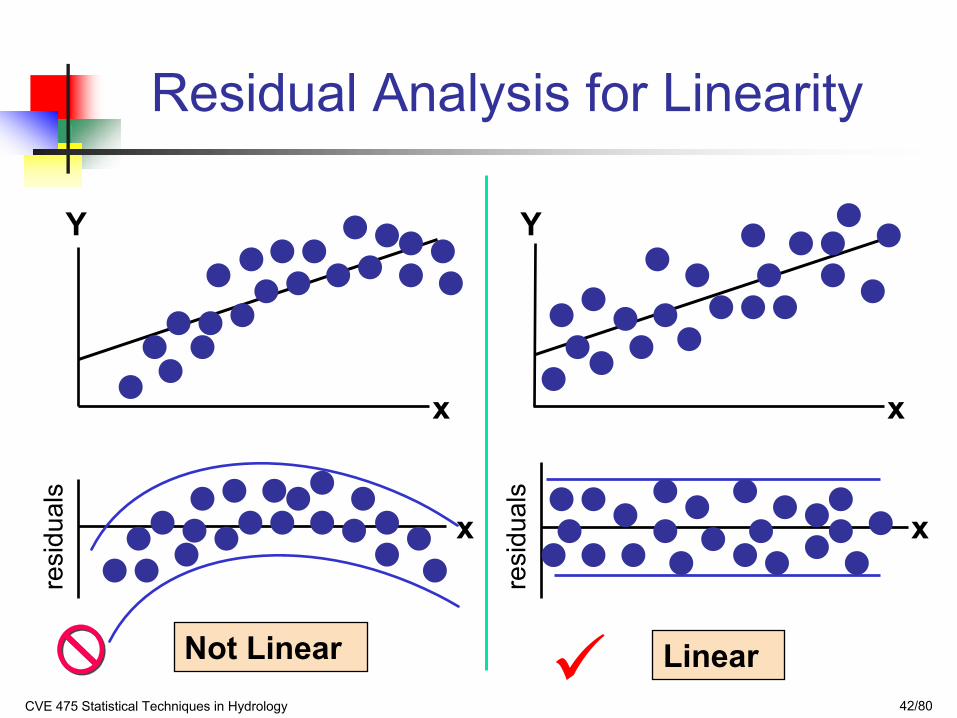
Residual Analysis for Linearity
Not Linear Linear
x
resi
dual
s
x
Y
x
Y
x
resi
dual
s
CVE 475 Statistical Techniques in Hydrology 43/80
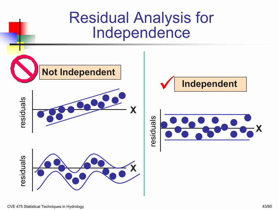
Residual Analysis for Independence
Not IndependentIndependent
X
Xresi
dual
s
resi
dual
s
X
resi
dual
s
CVE 475 Statistical Techniques in Hydrology 44/80
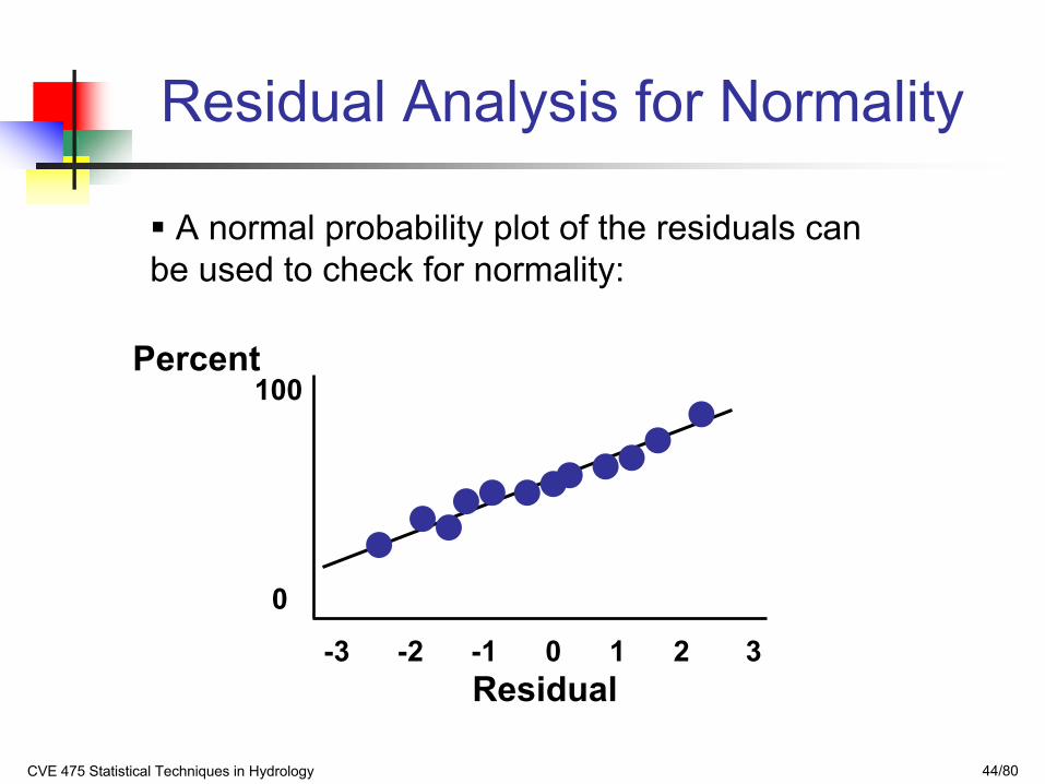
Residual Analysis for Normality
Percent
Residual
A normal probability plot of the residuals can be used to check for normality:
-3 -2 -1 0 1 2 3
0
100
CVE 475 Statistical Techniques in Hydrology 45/80
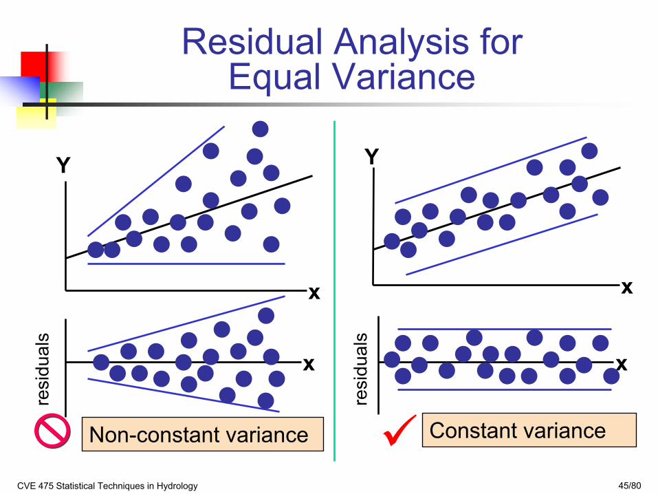
Residual Analysis for Equal Variance
Non-constant variance Constant variance
x x
Y
x x
Y
resi
dual
s
resi
dual
s
CVE 475 Statistical Techniques in Hydrology 46/80
House Price Model Residual Plot
-60
-40
-20
0
20
40
60
80
0 1000 2000 3000
Square Feet
Res
idua
ls
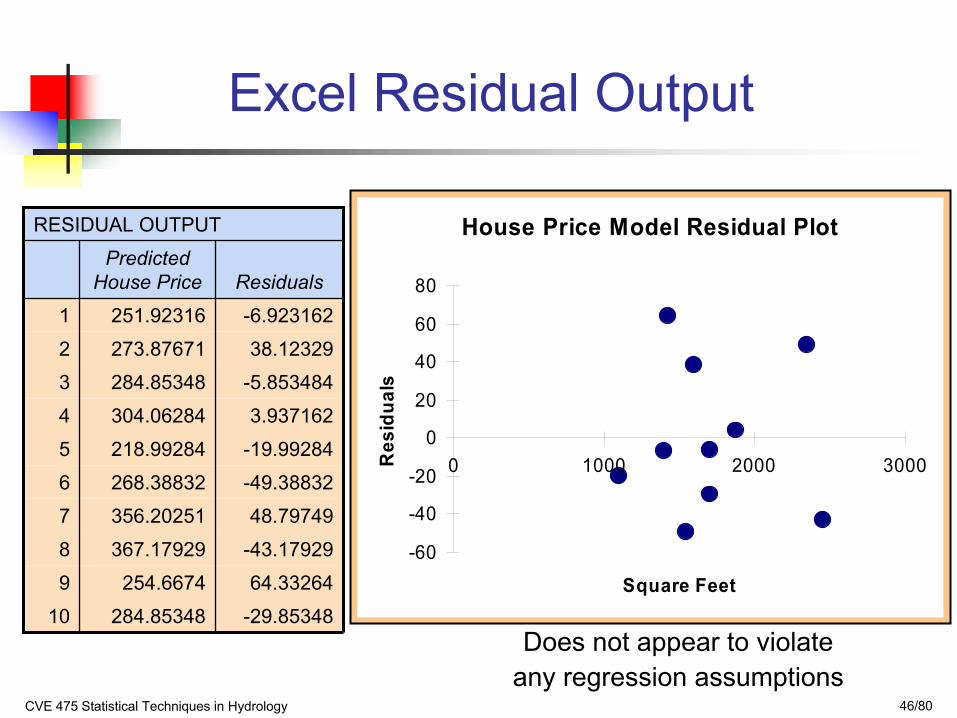
Excel Residual Output
-29.85348284.8534810
64.33264254.66749
-43.17929367.179298
48.79749356.202517
-49.38832268.388326
-19.99284218.992845
3.937162304.062844
-5.853484284.853483
38.12329273.876712
-6.923162251.923161
ResidualsPredicted
House Price
RESIDUAL OUTPUT
Does not appear to violate any regression assumptions
CVE 475 Statistical Techniques in Hydrology 47/80
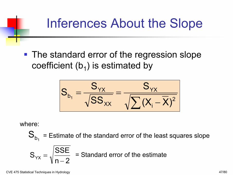
Inferences About the Slope
The standard error of the regression slope coefficient (b1) is estimated by
∑ −==
2i
YX
XX
YXb
)X(X
SSSSS
1
where:
= Estimate of the standard error of the least squares slope
= Standard error of the estimate
1bS
2nSSESYX −
=
CVE 475 Statistical Techniques in Hydrology 48/80
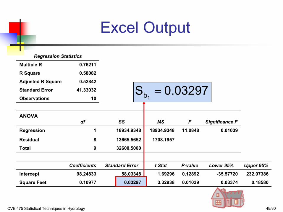
Excel Output
0.185800.033740.010393.329380.032970.10977Square Feet
232.07386-35.577200.128921.6929658.0334898.24833Intercept
Upper 95%Lower 95%P-valuet StatStandard ErrorCoefficients
32600.50009Total
1708.195713665.56528Residual
0.0103911.084818934.934818934.93481Regression
Significance FFMSSSdfANOVA
10Observations
41.33032Standard Error
0.52842Adjusted R Square
0.58082R Square
0.76211Multiple R
Regression Statistics
0.03297S1b =
CVE 475 Statistical Techniques in Hydrology 49/80
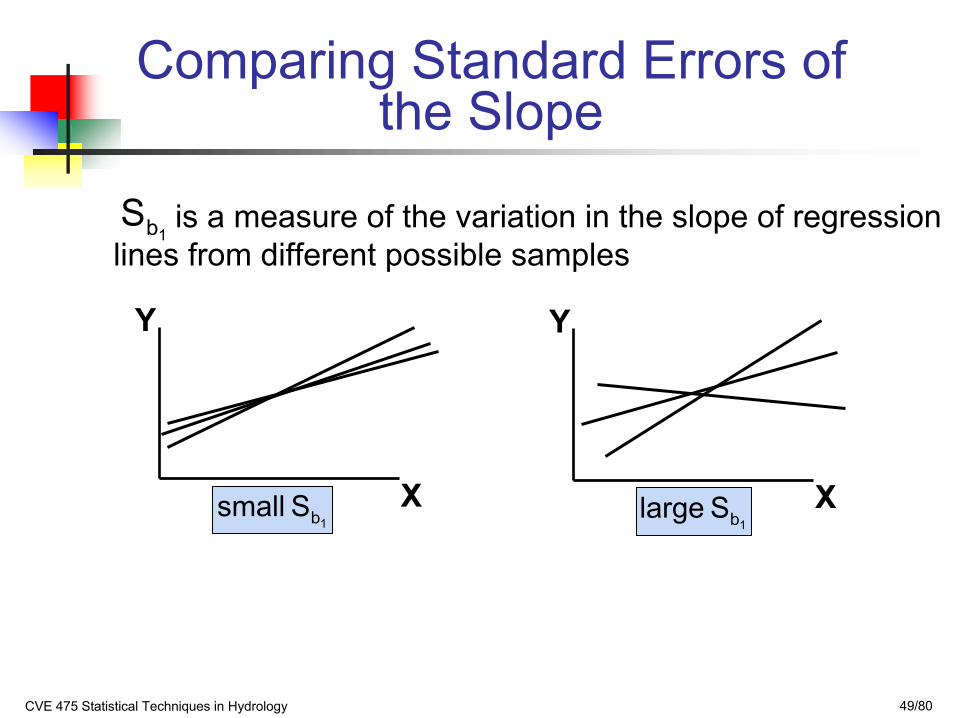
Comparing Standard Errors of the Slope
Y
X
Y
X1bS small
1bS large
is a measure of the variation in the slope of regression lines from different possible samples
1bS
CVE 475 Statistical Techniques in Hydrology 50/80
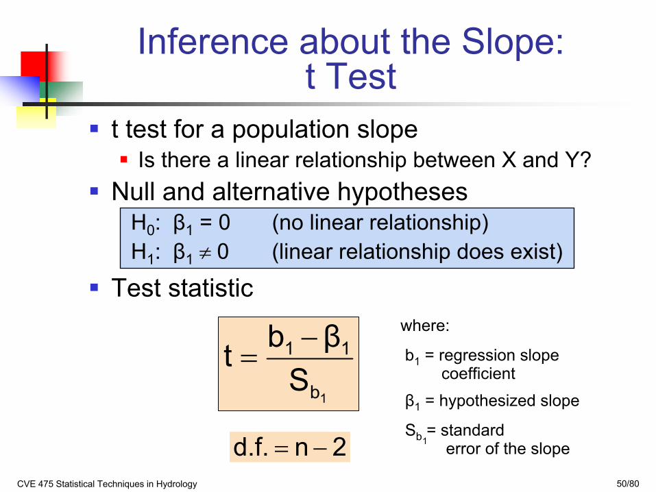
Inference about the Slope: t Test
t test for a population slopeIs there a linear relationship between X and Y?
Null and alternative hypothesesH0: β1 = 0 (no linear relationship)H1: β1 ≠ 0 (linear relationship does exist)
Test statistic
1b
11
Sβbt −
=
2nd.f. −=
where:
b1 = regression slopecoefficient
β1 = hypothesized slope
Sb = standarderror of the slope1
CVE 475 Statistical Techniques in Hydrology 51/80
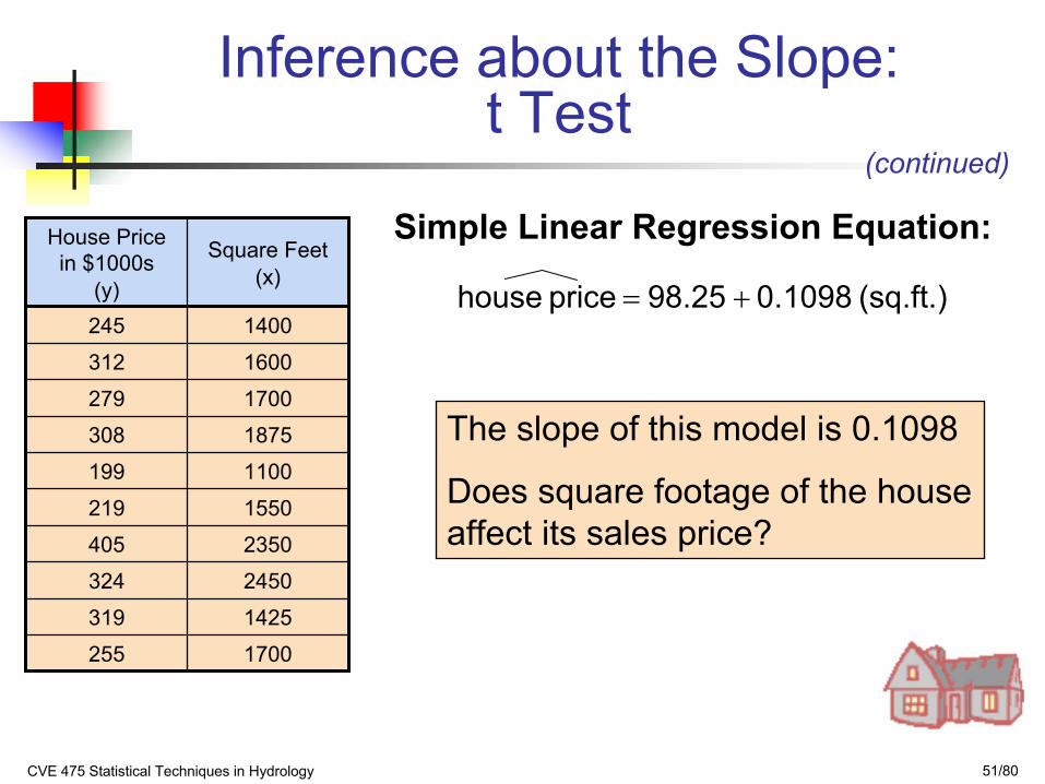
1700255
1425319
2450324
2350405
1550219
1100199
1875308
1700279
1600312
1400245
Square Feet (x)
House Price in $1000s
(y) (sq.ft.) 0.1098 98.25 price house +=
Simple Linear Regression Equation:
The slope of this model is 0.1098
Does square footage of the house affect its sales price?
Inference about the Slope: t Test
(continued)
CVE 475 Statistical Techniques in Hydrology 52/80
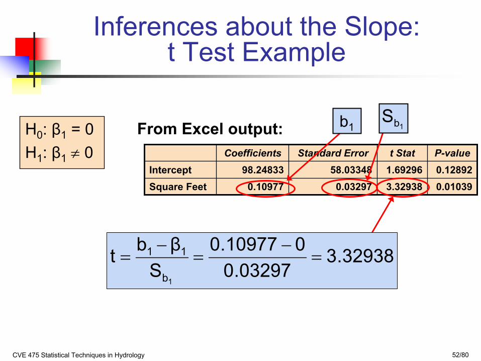
Inferences about the Slope: t Test Example
H0: β1 = 0H1: β1 ≠ 0
From Excel output:
0.010393.329380.032970.10977Square Feet0.128921.6929658.0334898.24833InterceptP-valuet StatStandard ErrorCoefficients
1bS
t
b1
32938.303297.0
010977.0Sβbt1b
11 =−
=−
=
CVE 475 Statistical Techniques in Hydrology 53/80
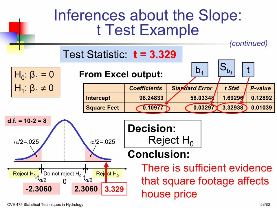
Inferences about the Slope: t Test Example
H0: β1 = 0H1: β1 ≠ 0
Test Statistic: t = 3.329
There is sufficient evidence that square footage affects house price
From Excel output:
Reject H0
0.010393.329380.032970.10977Square Feet0.128921.6929658.0334898.24833InterceptP-valuet StatStandard ErrorCoefficients
1bS tb1
Decision:
Conclusion:Reject H0Reject H0
α/2=.025
-tα/2Do not reject H0
0 tα/2
α/2=.025
-2.3060 2.3060 3.329
d.f. = 10-2 = 8
(continued)
CVE 475 Statistical Techniques in Hydrology 54/80
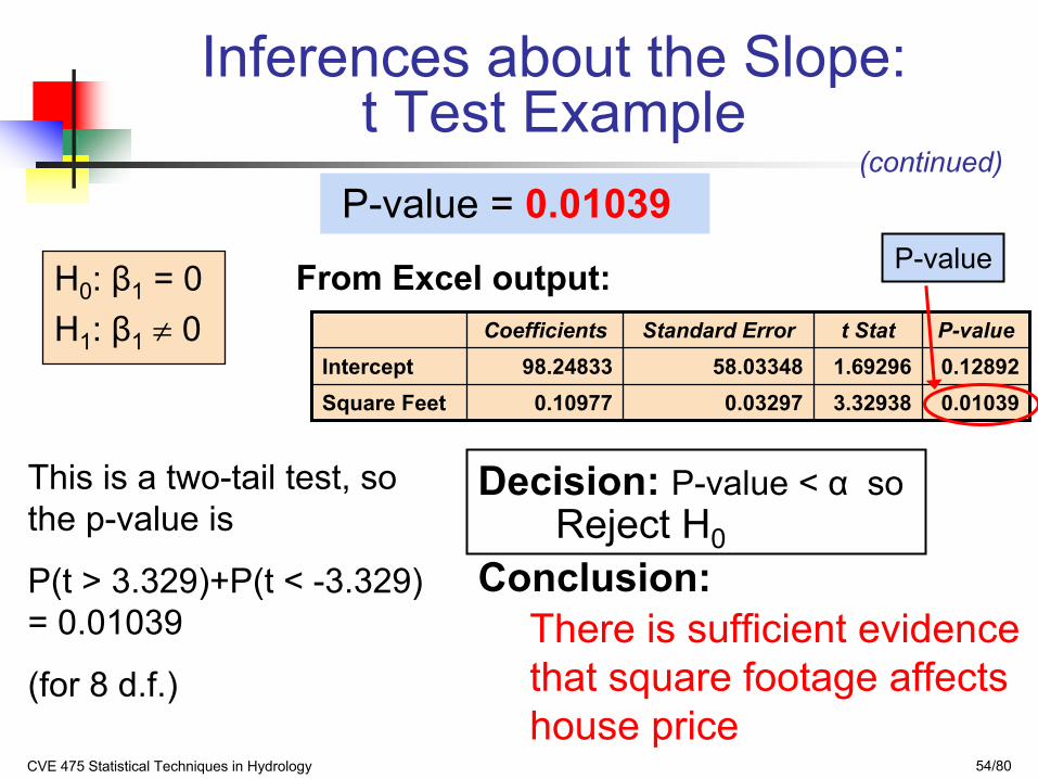
Inferences about the Slope: t Test Example
H0: β1 = 0H1: β1 ≠ 0
P-value = 0.01039
There is sufficient evidence that square footage affects house price
From Excel output:
Reject H0
0.010393.329380.032970.10977Square Feet0.128921.6929658.0334898.24833InterceptP-valuet StatStandard ErrorCoefficients
P-value
Decision: P-value < α so
Conclusion:
(continued)
This is a two-tail test, so the p-value is
P(t > 3.329)+P(t < -3.329) = 0.01039
(for 8 d.f.)
CVE 475 Statistical Techniques in Hydrology 55/80
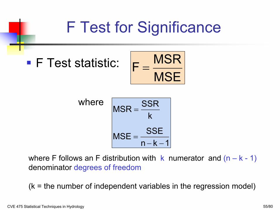
F Test for Significance
F Test statistic:
where
MSEMSRF =
1knSSEMSE
kSSRMSR
−−=
=
where F follows an F distribution with k numerator and (n – k - 1)denominator degrees of freedom
(k = the number of independent variables in the regression model)
CVE 475 Statistical Techniques in Hydrology 56/80
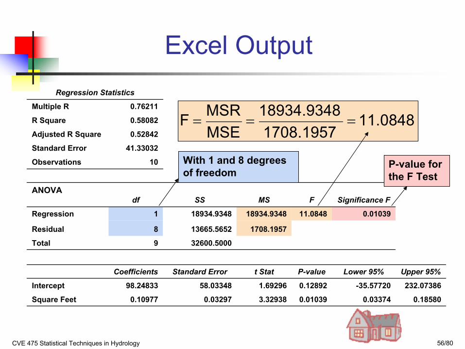
Excel Output
0.185800.033740.010393.329380.032970.10977Square Feet
232.07386-35.577200.128921.6929658.0334898.24833Intercept
Upper 95%Lower 95%P-valuet StatStandard ErrorCoefficients
32600.50009Total
1708.195713665.56528Residual
0.0103911.084818934.934818934.93481Regression
Significance FFMSSSdfANOVA
10Observations
41.33032Standard Error
0.52842Adjusted R Square
0.58082R Square
0.76211Multiple R
Regression Statistics
11.08481708.1957
18934.9348MSEMSRF ===
With 1 and 8 degrees of freedom
P-value for the F Test
CVE 475 Statistical Techniques in Hydrology 57/80
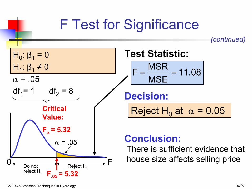
H0: β1 = 0H1: β1 ≠ 0α = .05df1= 1 df2 = 8
Test Statistic:
Decision:
Conclusion:
Reject H0 at α = 0.05
There is sufficient evidence that house size affects selling price0
α = .05
F.05 = 5.32Reject H0Do not
reject H0
11.08MSEMSRF ==
Critical Value:
Fα = 5.32
F Test for Significance(continued)
F
CVE 475 Statistical Techniques in Hydrology 58/80
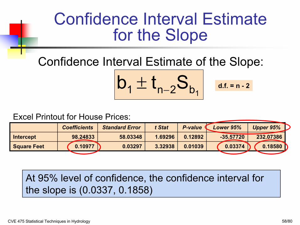
Confidence Interval Estimate for the Slope
Confidence Interval Estimate of the Slope:
Excel Printout for House Prices:
At 95% level of confidence, the confidence interval for the slope is (0.0337, 0.1858)
1b2n1 Stb −±
0.185800.033740.010393.329380.032970.10977Square Feet
232.07386-35.577200.128921.6929658.0334898.24833Intercept
Upper 95%Lower 95%P-valuet StatStandard ErrorCoefficients
d.f. = n - 2
CVE 475 Statistical Techniques in Hydrology 59/80
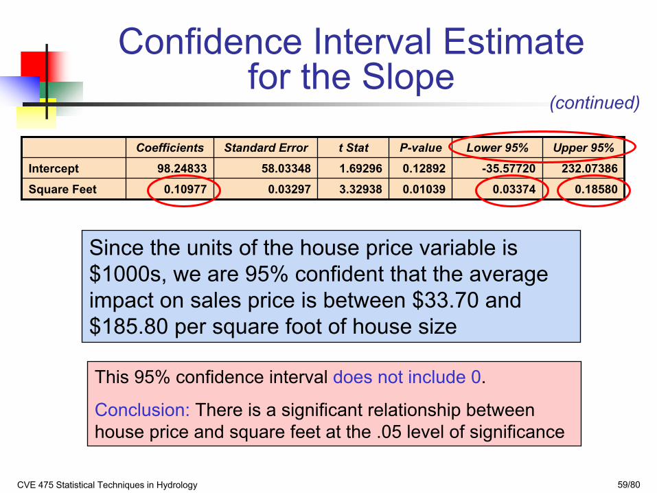
Since the units of the house price variable is $1000s, we are 95% confident that the average impact on sales price is between $33.70 and $185.80 per square foot of house size
0.185800.033740.010393.329380.032970.10977Square Feet
232.07386-35.577200.128921.6929658.0334898.24833Intercept
Upper 95%Lower 95%P-valuet StatStandard ErrorCoefficients
This 95% confidence interval does not include 0.
Conclusion: There is a significant relationship between house price and square feet at the .05 level of significance
Confidence Interval Estimate for the Slope
(continued)
CVE 475 Statistical Techniques in Hydrology 60/80
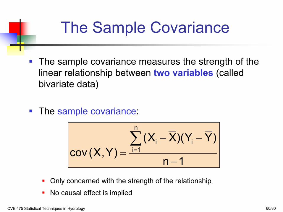
The Sample Covariance
The sample covariance measures the strength of the linear relationship between two variables (called bivariate data)
The sample covariance:
Only concerned with the strength of the relationship
No causal effect is implied
1n
)YY)(XX()Y,X(cov
n
1iii
−
−−=∑=
CVE 475 Statistical Techniques in Hydrology 61/80
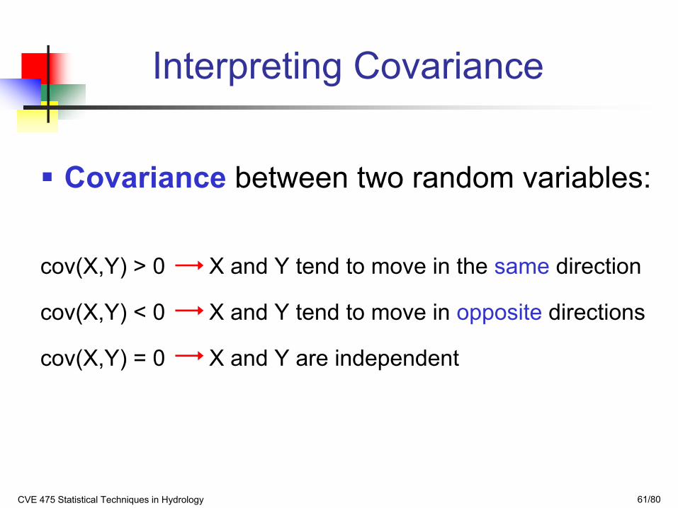
Covariance between two random variables:
cov(X,Y) > 0 X and Y tend to move in the same direction
cov(X,Y) < 0 X and Y tend to move in opposite directions
cov(X,Y) = 0 X and Y are independent
Interpreting Covariance
CVE 475 Statistical Techniques in Hydrology 62/80
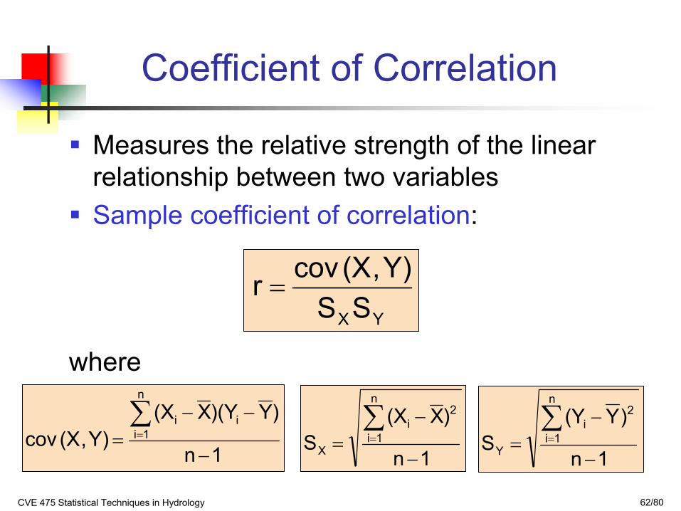
Coefficient of Correlation
Measures the relative strength of the linear relationship between two variablesSample coefficient of correlation:
where
YXSSY),(Xcovr =
1n
)X(XS
n
1i
2i
X −
−=∑=
1n
)Y)(YX(XY),(Xcov
n
1iii
−
−−=∑=
1n
)Y(YS
n
1i
2i
Y −
−=∑=
CVE 475 Statistical Techniques in Hydrology 63/80
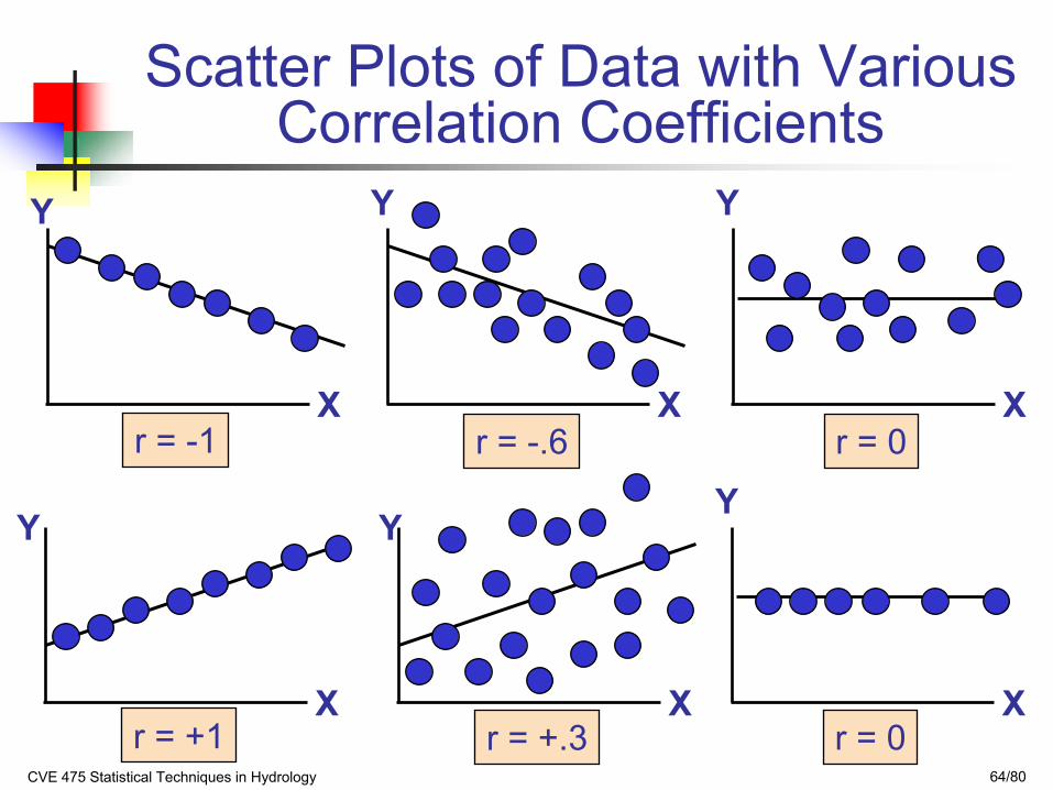
Features of Correlation Coefficient, r
Unit free
Ranges between –1 and 1
The closer to –1, the stronger the negative linear relationship
The closer to 1, the stronger the positive linear relationship
The closer to 0, the weaker the linear relationship
CVE 475 Statistical Techniques in Hydrology 64/80
Scatter Plots of Data with Various Correlation Coefficients
Y
X
Y
X
Y
X
Y
X
Y
X
r = -1 r = -.6 r = 0
r = +.3r = +1
Y
Xr = 0
CVE 475 Statistical Techniques in Hydrology 65/80
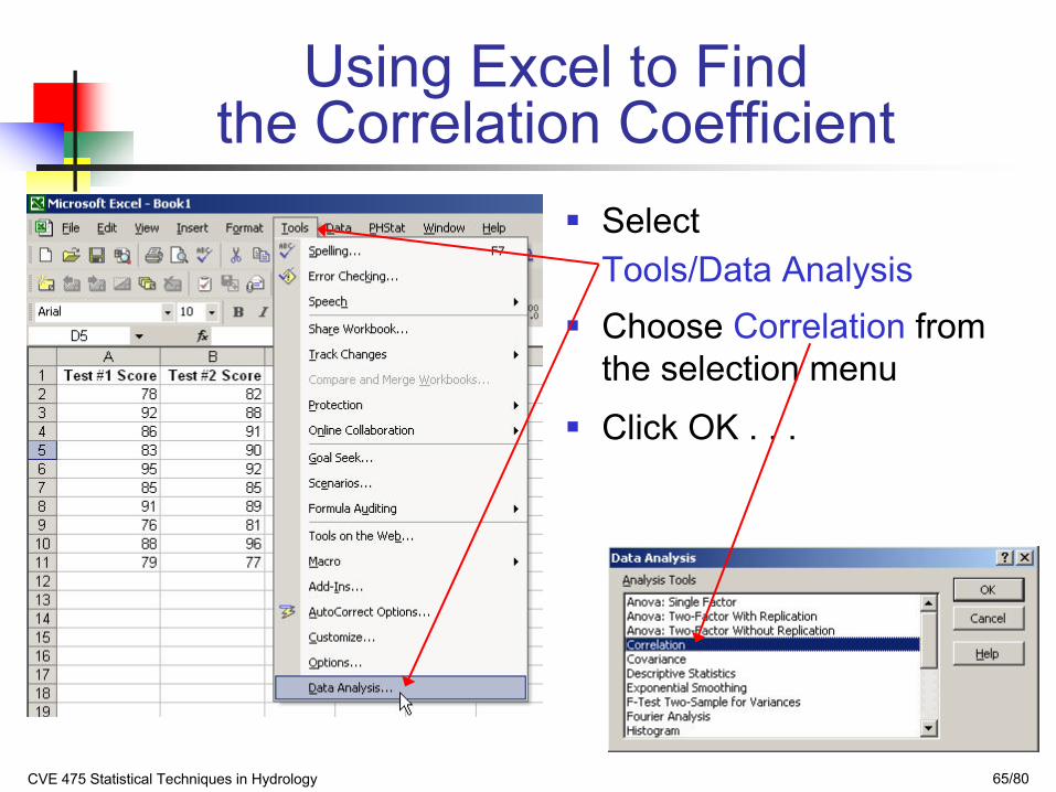
Using Excel to Find the Correlation Coefficient
Select Tools/Data AnalysisChoose Correlation from the selection menu
Click OK . . .
CVE 475 Statistical Techniques in Hydrology 66/80
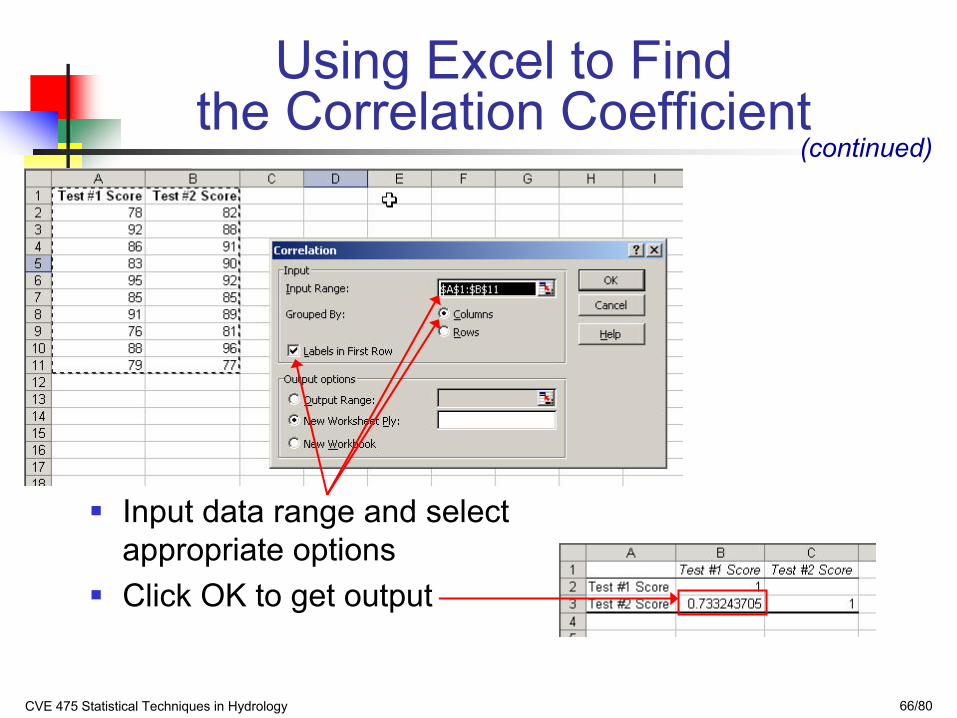
Using Excel to Find the Correlation Coefficient
Input data range and select appropriate optionsClick OK to get output
(continued)
CVE 475 Statistical Techniques in Hydrology 67/80
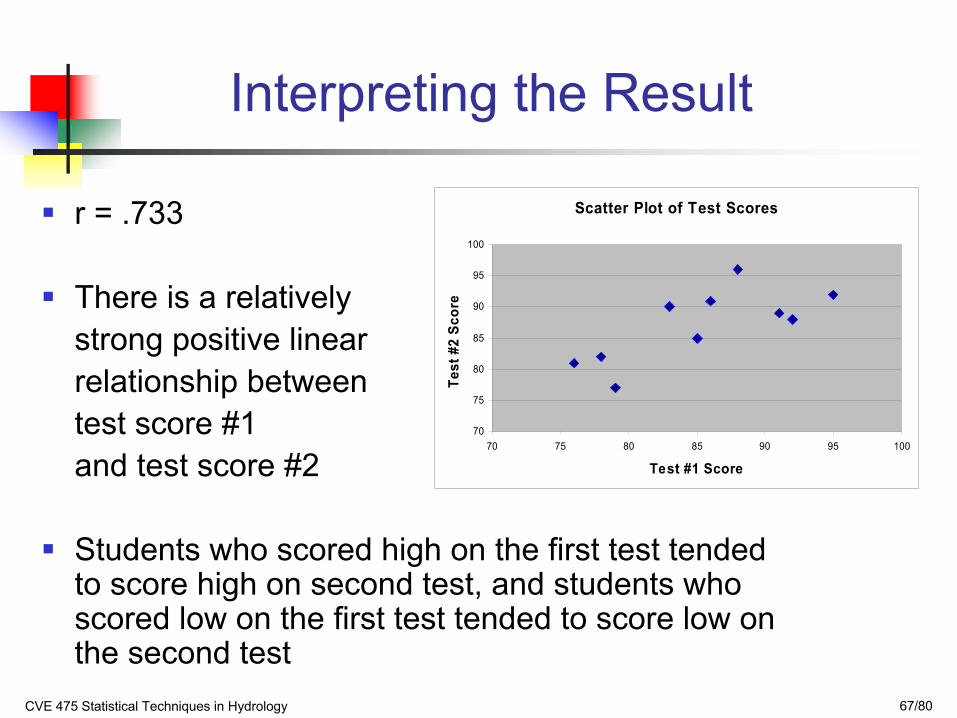
Interpreting the Result
r = .733
There is a relatively strong positive linear relationship between test score #1 and test score #2
Students who scored high on the first test tended to score high on second test, and students who scored low on the first test tended to score low on the second test
Scatter Plot of Test Scores
70
75
80
85
90
95
100
70 75 80 85 90 95 100
Test #1 ScoreTe
st #
2 Sc
ore
CVE 475 Statistical Techniques in Hydrology 68/80
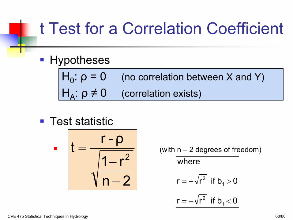
t Test for a Correlation Coefficient
Hypotheses H0: ρ = 0 (no correlation between X and Y)
HA: ρ ≠ 0 (correlation exists)
Test statistic
(with n – 2 degrees of freedom)
2nr1ρ-rt
2
−−
=
0 b if rr
0 b if rr
where
12
12
<−=
>+=
CVE 475 Statistical Techniques in Hydrology 69/80
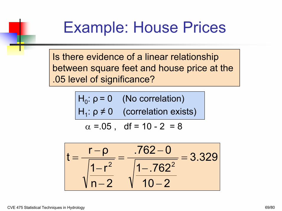
Example: House Prices
Is there evidence of a linear relationship between square feet and house price at the .05 level of significance?
H0: ρ = 0 (No correlation)H1: ρ ≠ 0 (correlation exists)α =.05 , df = 10 - 2 = 8
3.329
210.7621
0.762
2nr1ρrt
22=
−−
−=
−−
−=
CVE 475 Statistical Techniques in Hydrology 70/80
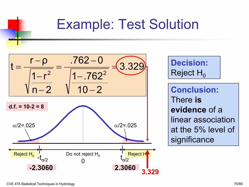
Example: Test Solution
Conclusion:There is evidence of a linear association at the 5% level of significance
Decision:Reject H0
Reject H0Reject H0
α/2=.025
-tα/2Do not reject H0
0 tα/2
α/2=.025
-2.3060 2.3060 3.329
d.f. = 10-2 = 8
3.329
210.7621
0.762
2nr1ρrt
22=
−−
−=
−−
−=
CVE 475 Statistical Techniques in Hydrology 71/80
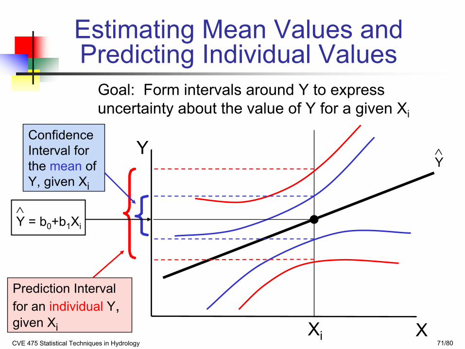
Estimating Mean Values and Predicting Individual Values
Y
XXi
Y = b0+b1Xi
∧
Confidence Interval for the mean of Y, given Xi
Prediction Interval for an individual Y,given Xi
Goal: Form intervals around Y to express uncertainty about the value of Y for a given Xi
Y∧
CVE 475 Statistical Techniques in Hydrology 72/80
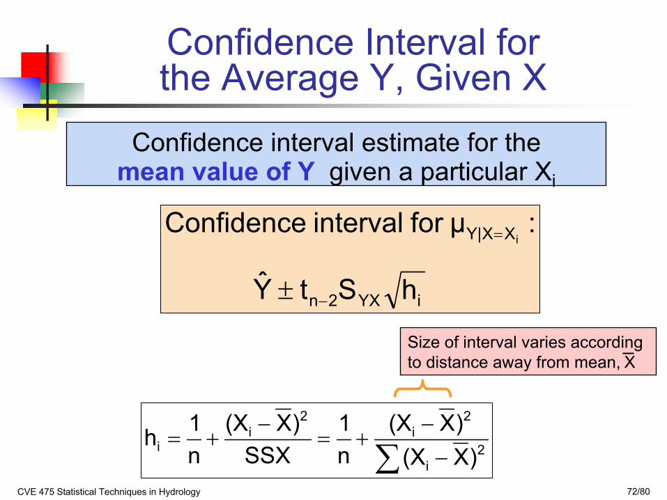
Confidence Interval for the Average Y, Given X
Confidence interval estimate for the mean value of Y given a particular Xi
Size of interval varies according to distance away from mean, X
iYX2n
XX|Y
hStY
:µ for interval Confidencei
−
=
±
∑ −−
+=−
+=2
i
2i
2i
i )X(X)X(X
n1
SSX)X(X
n1h
CVE 475 Statistical Techniques in Hydrology 73/80
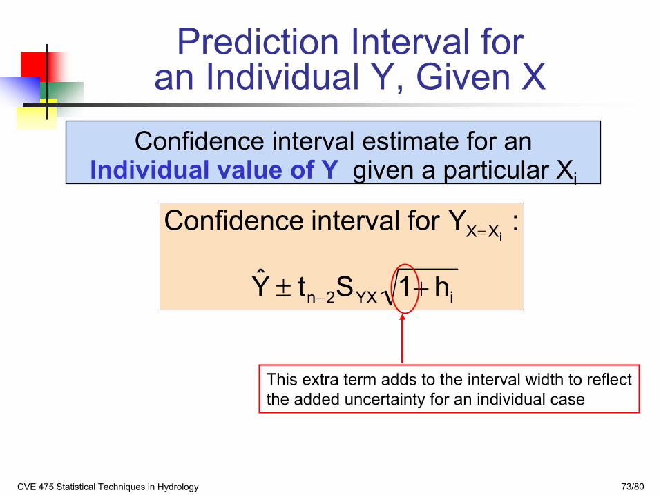
Prediction Interval for an Individual Y, Given X
Confidence interval estimate for an Individual value of Y given a particular Xi
This extra term adds to the interval width to reflect the added uncertainty for an individual case
iYX2n
XX
h1StY
: Yfor interval Confidencei
+± −
=
CVE 475 Statistical Techniques in Hydrology 74/80
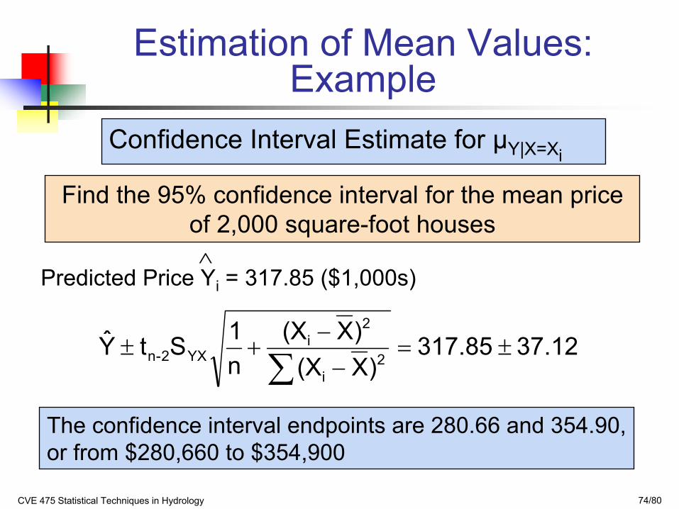
Estimation of Mean Values: Example
Find the 95% confidence interval for the mean price of 2,000 square-foot houses
Predicted Price Yi = 317.85 ($1,000s)∧
Confidence Interval Estimate for µY|X=X
37.12317.85)X(X
)X(Xn1StY
2i
2i
YX2-n ±=−
−+±∑
The confidence interval endpoints are 280.66 and 354.90, or from $280,660 to $354,900
i
CVE 475 Statistical Techniques in Hydrology 75/80
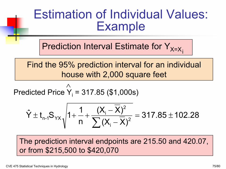
Estimation of Individual Values: Example
Find the 95% prediction interval for an individual house with 2,000 square feet
Predicted Price Yi = 317.85 ($1,000s)∧
Prediction Interval Estimate for YX=X
102.28317.85)X(X
)X(Xn11StY
2i
2i
YX1-n ±=−
−++±∑
The prediction interval endpoints are 215.50 and 420.07, or from $215,500 to $420,070
i
CVE 475 Statistical Techniques in Hydrology 76/80
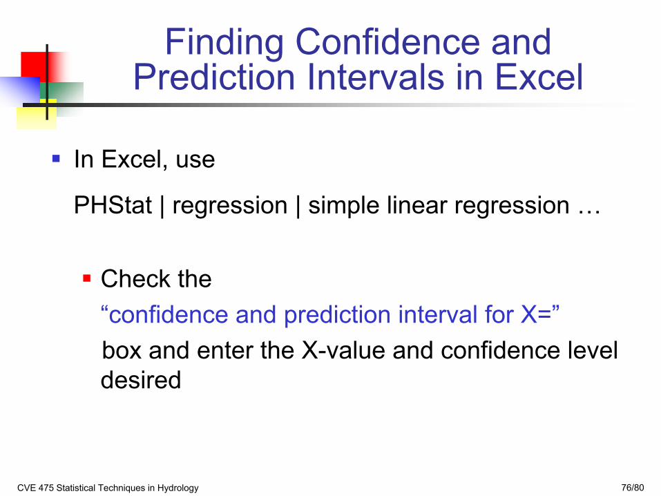
Finding Confidence and Prediction Intervals in Excel
In Excel, use
PHStat | regression | simple linear regression …
Check the “confidence and prediction interval for X=”box and enter the X-value and confidence level desired
CVE 475 Statistical Techniques in Hydrology 77/80
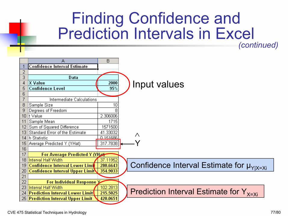
Input values
Finding Confidence and Prediction Intervals in Excel
(continued)
Confidence Interval Estimate for µY|X=Xi
Prediction Interval Estimate for YX=Xi
Y ∧
CVE 475 Statistical Techniques in Hydrology 78/80
Pitfalls of Regression Analysis
Lacking an awareness of the assumptions underlying least-squares regressionNot knowing how to evaluate the assumptionsNot knowing the alternatives to least-squares regression if a particular assumption is violatedUsing a regression model without knowledge of the subject matterExtrapolating outside the relevant range
CVE 475 Statistical Techniques in Hydrology 79/80
Strategies for Avoiding the Pitfalls of Regression
Start with a scatter diagram of X vs. Y to observe possible relationshipPerform residual analysis to check the assumptions
Plot the residuals vs. X to check for violations of assumptions such as homoscedasticityUse a histogram, stem-and-leaf display, box-and-whisker plot, or normal probability plot of the residuals to uncover possible non-normality
CVE 475 Statistical Techniques in Hydrology 80/80
Strategies for Avoiding the Pitfalls of Regression
If there is violation of any assumption, use alternative methods or modelsIf there is no evidence of assumption violation, then test for the significance of the regression coefficients and construct confidence intervals and prediction intervalsAvoid making predictions or forecasts outside the relevant range
(continued)


![[Hydrology] groundwater hydrology david k. todd (2005)](https://img.pdfslide.us/doc/110x75/55a8e6001a28ab6c2f8b4687/hydrology-groundwater-hydrology-david-k-todd-2005-55b0d9a792c06.jpg)