Statistical Analysis of the Statistical Analysis of the Regression-Discontinuity DesignRegression-Discontinuity Design

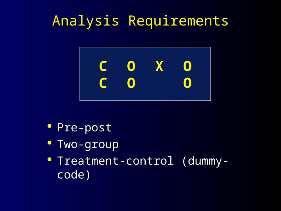
Analysis RequirementsAnalysis Requirements

Pre-postPre-post Two-groupTwo-group Treatment-control (dummy-code)Treatment-control (dummy-code)

C O X OC O O

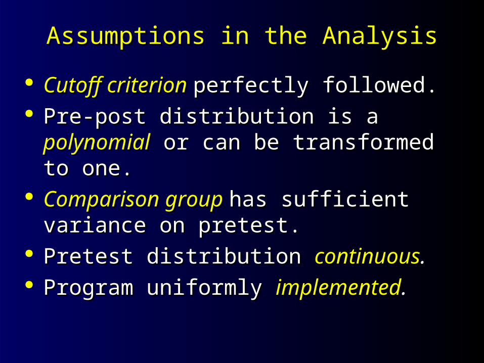
Assumptions in the AnalysisAssumptions in the Analysis

Cutoff criterionCutoff criterion perfectly followed.perfectly followed. Pre-post distribution is a Pre-post distribution is a polynomialpolynomial or can or can

be transformed to one.be transformed to one. Comparison groupComparison group has sufficient variance has sufficient variance

on pretest.on pretest. Pretest distribution Pretest distribution continuouscontinuous.. Program uniformly Program uniformly implementedimplemented..

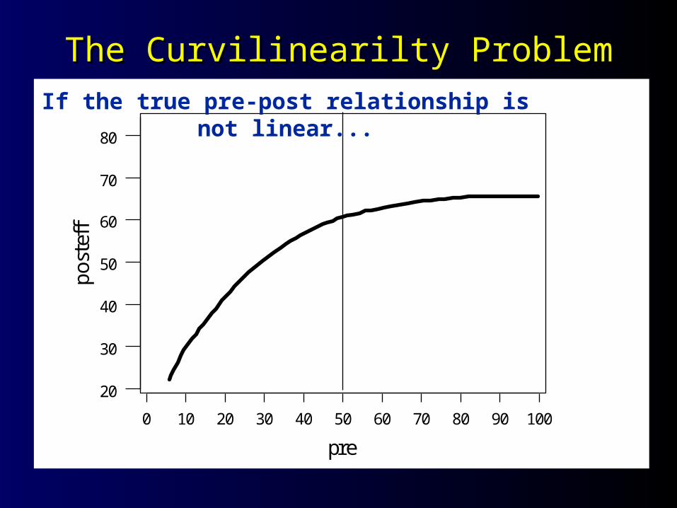
The Curvilinearilty ProblemThe Curvilinearilty Problem

1009080706050403020100

80

70

60

50

40

30

20

pre

po

ste

ffIf the true pre-post relationship is not linear...

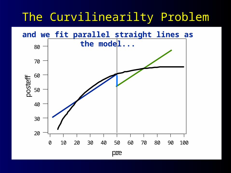
The Curvilinearilty ProblemThe Curvilinearilty Problem

1009080706050403020100

80

70

60

50

40

30

20

pre

po

ste

ffand we fit parallel straight lines as the model...

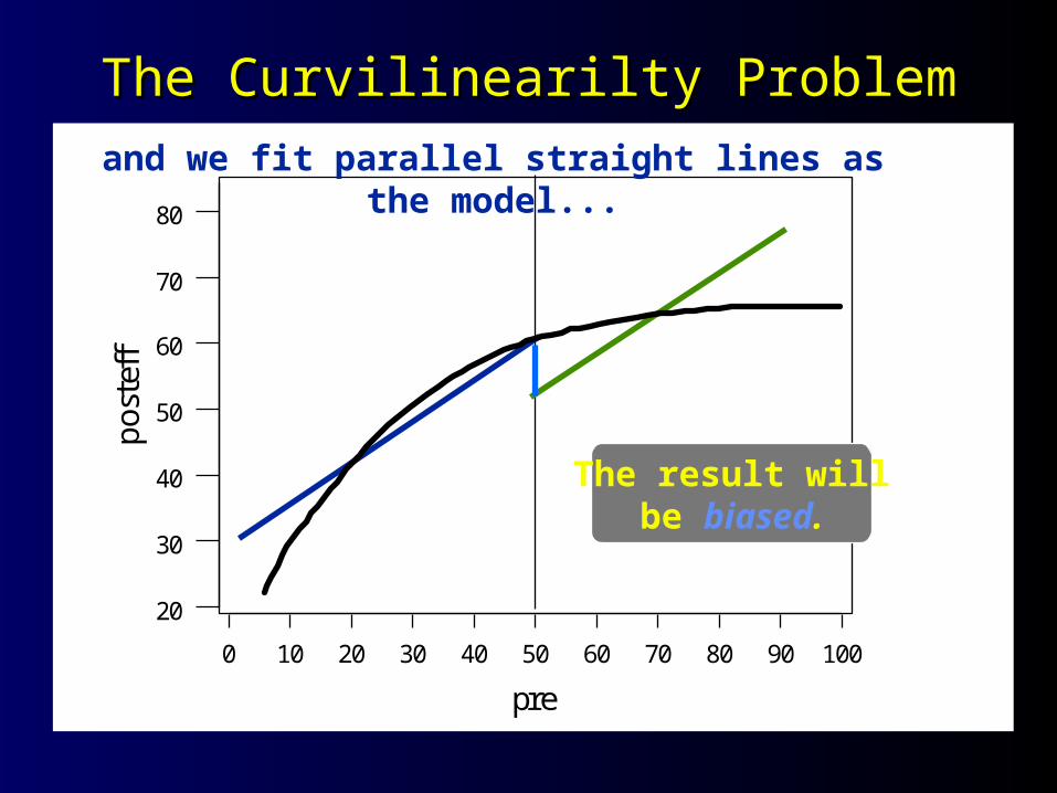
The Curvilinearilty ProblemThe Curvilinearilty Problem

1009080706050403020100

80

70

60

50

40

30

20

pre

po

ste

ffand we fit parallel straight lines as the model...

The result willbe biased.

The Curvilinearilty ProblemThe Curvilinearilty Problem

1009080706050403020100

80

70

60

50

40

30

20

pre

po

ste

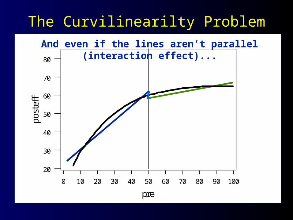
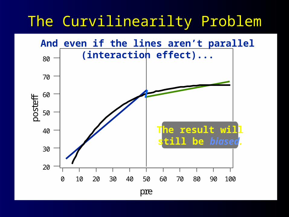
ffAnd even if the lines aren’t parallel (interaction effect)...

The Curvilinearilty ProblemThe Curvilinearilty Problem

1009080706050403020100

80

70

60

50

40

30

20

pre

po

ste

ffAnd even if the lines aren’t parallel (interaction effect)...

The result willstill be biased.

Model SpecificationModel Specification

If you specify the model If you specify the model exactlyexactly, there is , there is no bias.no bias.

If you If you overspecifyoverspecify the model (add more the model (add more terms than needed), the result is terms than needed), the result is unbiased, but inefficientunbiased, but inefficient

If you If you underspecifyunderspecify the model (omit one the model (omit one or more necessary terms, the result is or more necessary terms, the result is biased.biased.

Model SpecificationModel Specification

yi = 0 + 1Xi + 2Zi

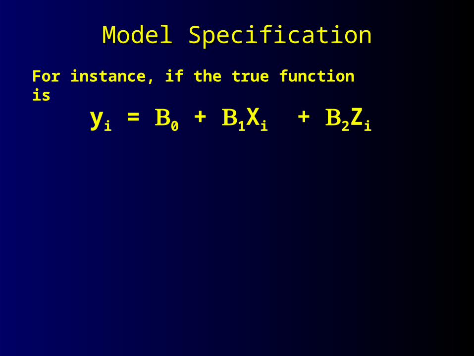
For instance, if the true function is

Model SpecificationModel Specification

yi = 0 + 1Xi + 2Zi

For instance, if the true function is

And we fit:

yi = 0 + 1Xi + 2Zi + ei

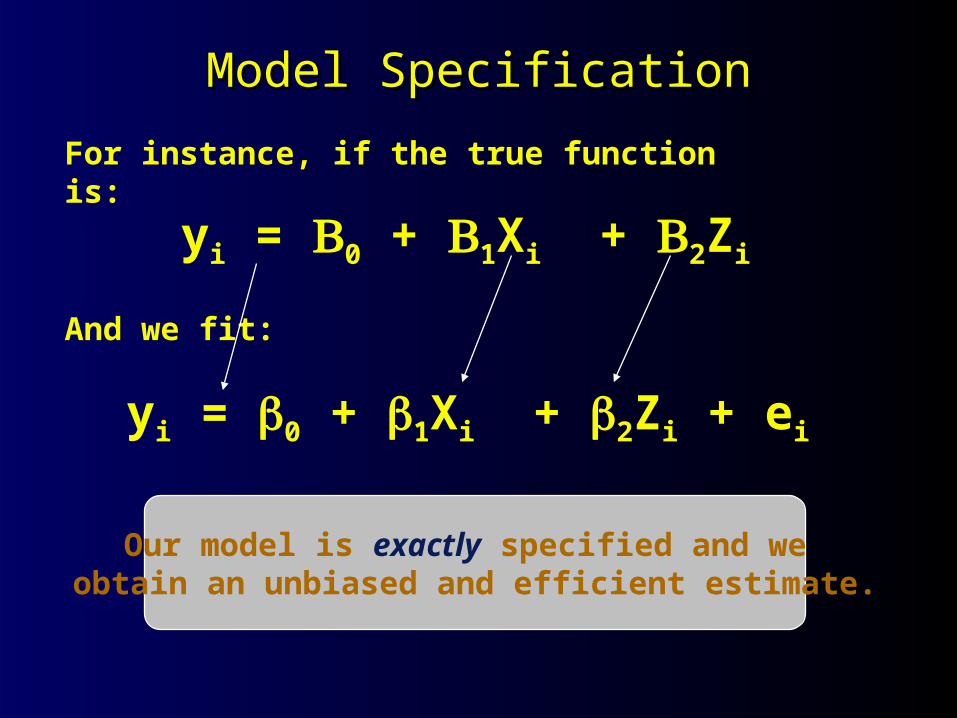
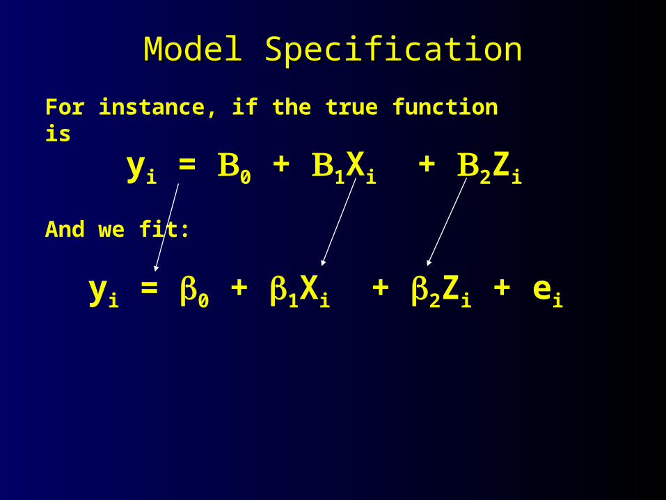
Model SpecificationModel Specification

yi = 0 + 1Xi + 2Zi

For instance, if the true function is:

And we fit:

yi = 0 + 1Xi + 2Zi + ei

Our model is exactly specified and we obtain an unbiased and efficient estimate.

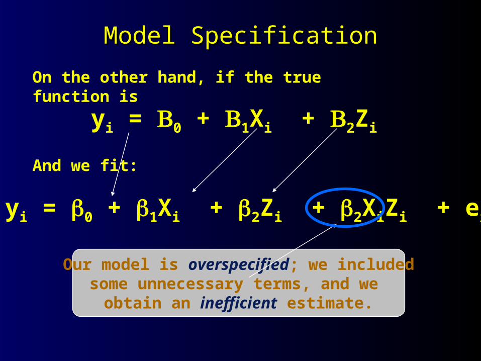
Model SpecificationModel Specification

yi = 0 + 1Xi + 2Zi

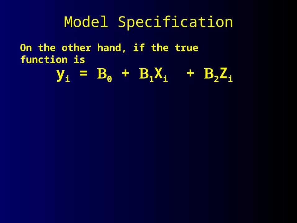
On the other hand, if the true function is

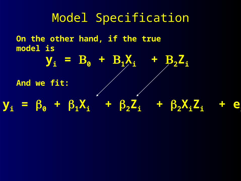
Model SpecificationModel Specification

yi = 0 + 1Xi + 2Zi

On the other hand, if the true model is

And we fit:

yi = 0 + 1Xi + 2Zi + 2XiZi + ei

Model SpecificationModel Specification

yi = 0 + 1Xi + 2Zi

On the other hand, if the true function is

And we fit:

yi = 0 + 1Xi + 2Zi + 2XiZi + ei

Our model is overspecified; we includedsome unnecessary terms, and we

obtain an inefficient estimate.

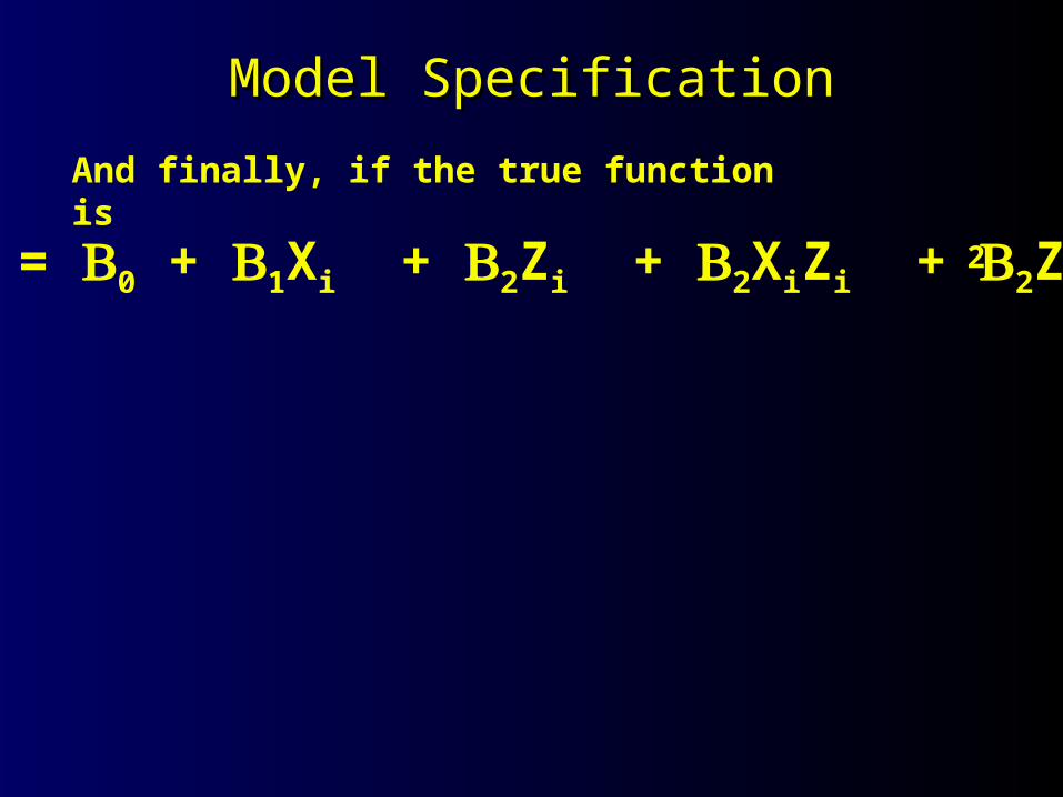
Model SpecificationModel Specification

yi = 0 + 1Xi + 2Zi + 2XiZi + 2Zi

And finally, if the true function is

2

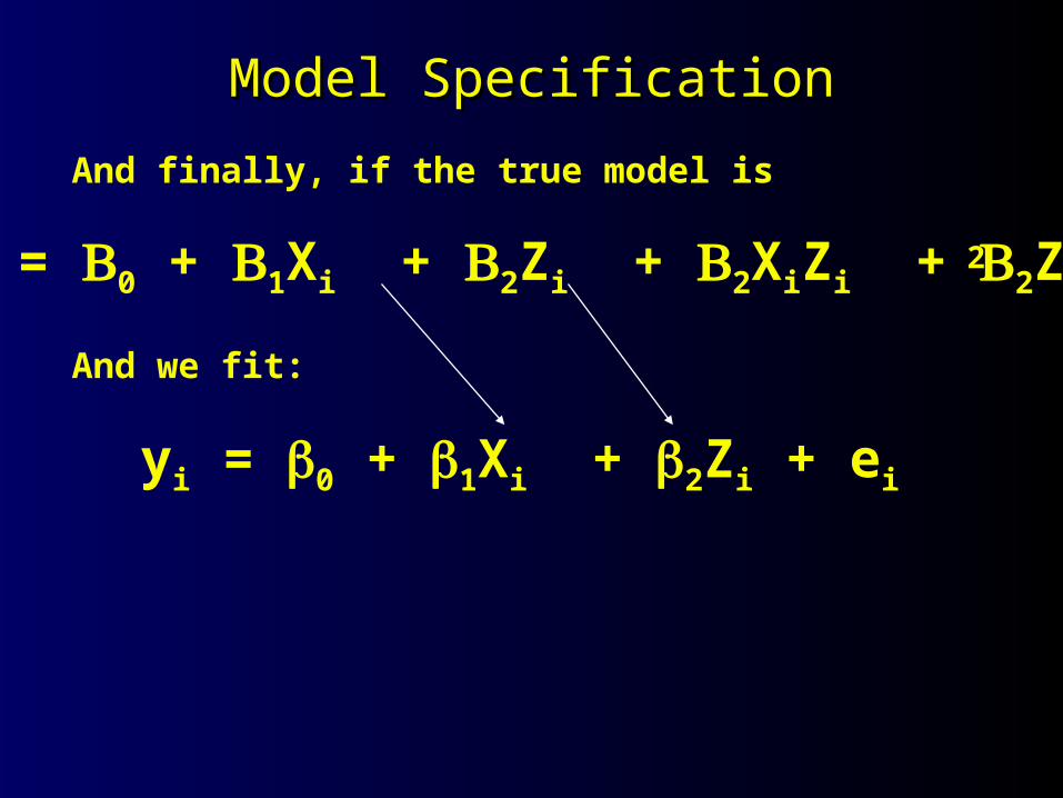
Model SpecificationModel Specification

yi = 0 + 1Xi + 2Zi + 2XiZi + 2Zi

And finally, if the true model is

And we fit:

yi = 0 + 1Xi + 2Zi + ei

2

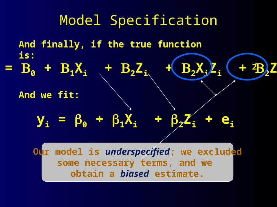
Model SpecificationModel Specification

yi = 0 + 1Xi + 2Zi + 2XiZi + 2Zi

And finally, if the true function is:

And we fit:

yi = 0 + 1Xi + 2Zi + ei

Our model is underspecified; we excludedsome necessary terms, and we

obtain a biased estimate.

2

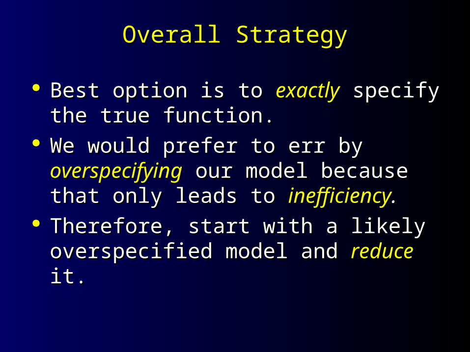
Overall StrategyOverall Strategy

Best option is to Best option is to exactlyexactly specify the true specify the true function.function.

We would prefer to err by We would prefer to err by overspecifyingoverspecifying our model because that only leads to our model because that only leads to inefficiencyinefficiency..

Therefore, start with a likely overspecified Therefore, start with a likely overspecified model and model and reducereduce it. it.

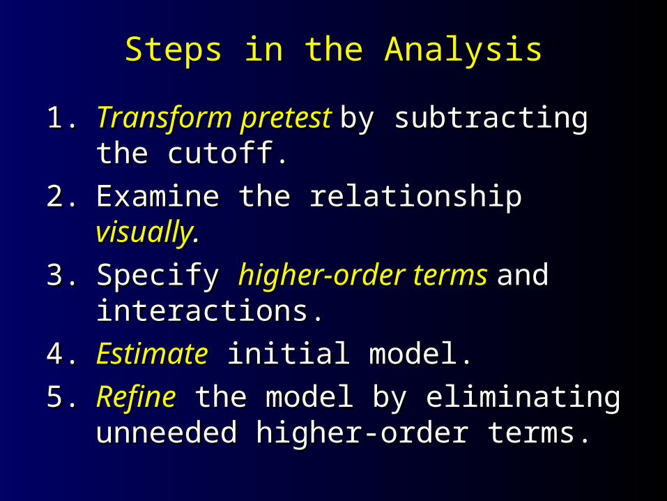
Steps in the AnalysisSteps in the Analysis

1.1. Transform pretestTransform pretest by subtracting the by subtracting the cutoff.cutoff.

2.2. Examine the relationship Examine the relationship visuallyvisually..

3.3. Specify Specify higher-order termshigher-order terms and and interactions.interactions.

4.4. EstimateEstimate initial model. initial model.

5.5. RefineRefine the model by eliminating the model by eliminating unneeded higher-order terms.unneeded higher-order terms.

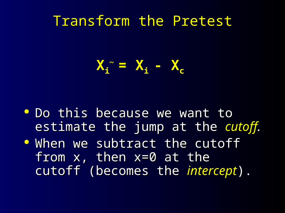
Transform the PretestTransform the Pretest

Do this because we want to estimate Do this because we want to estimate the jump at the the jump at the cutoffcutoff..

When we subtract the cutoff from x, When we subtract the cutoff from x, then x=0 at the cutoff (becomes the then x=0 at the cutoff (becomes the interceptintercept).).

Xi = Xi - Xc~

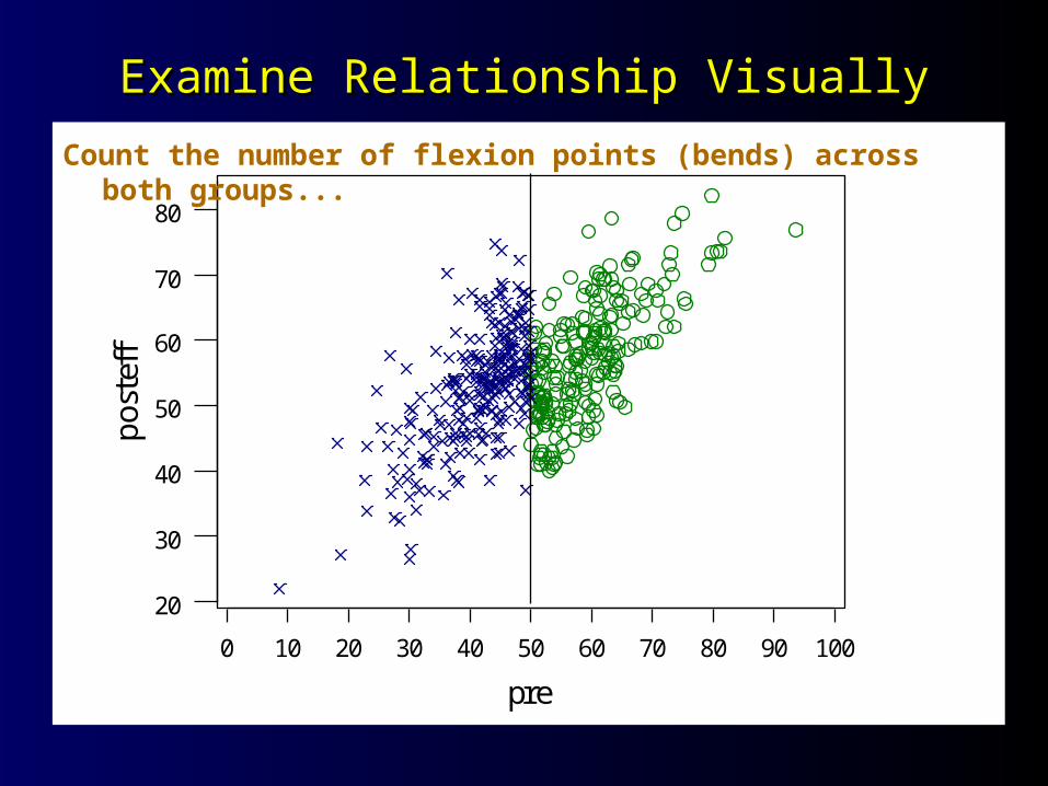
Examine Relationship VisuallyExamine Relationship Visually

1009080706050403020100

80

70

60

50

40

30

20

pre

po

ste

ffCount the number of flexion points (bends) across both groups...

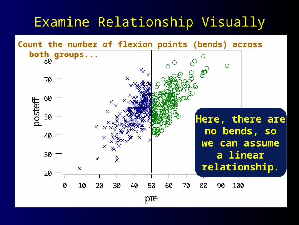
Examine Relationship VisuallyExamine Relationship Visually

1009080706050403020100

80

70

60

50

40

30

20

pre

po

ste

ff

Here, there areno bends, so

we can assumea linear

relationship.

Count the number of flexion points (bends) across both groups...

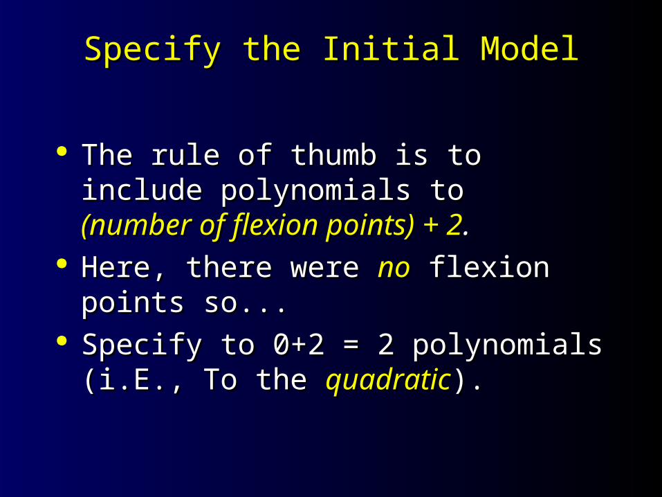
Specify the Initial ModelSpecify the Initial Model

The rule of thumb is to include The rule of thumb is to include polynomials topolynomials to(number of flexion points) + 2(number of flexion points) + 2..

Here, there were Here, there were nono flexion points so... flexion points so... Specify to 0+2 = 2 polynomials (i.E., To Specify to 0+2 = 2 polynomials (i.E., To

the the quadraticquadratic).).

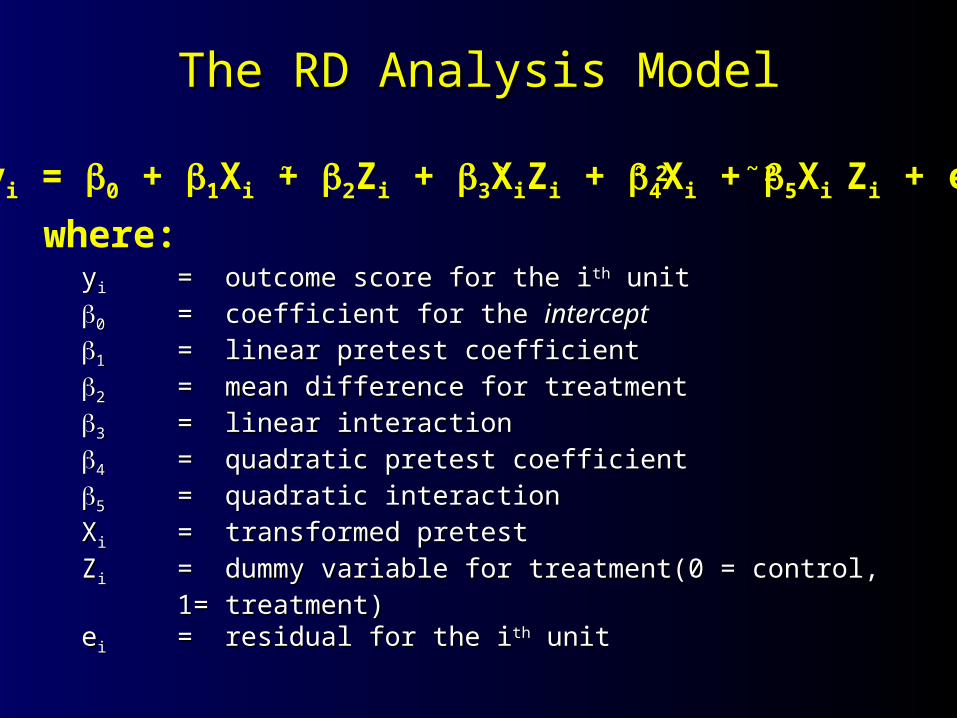
yi = 0 + 1Xi + 2Zi + 3XiZi + 4Xi + 5Xi Zi + ei

The RD Analysis ModelThe RD Analysis Model

yyii = = outcome score for the ioutcome score for the ithth unit unit

00 == coefficient for the coefficient for the interceptintercept

11 == linear pretest coefficientlinear pretest coefficient

22 == mean difference for treatmentmean difference for treatment

33 == linear interactionlinear interaction

44 == quadratic pretest coefficientquadratic pretest coefficient

55 == quadratic interactionquadratic interaction

XXii == transformed pretesttransformed pretest

ZZii == dummy variable for treatment(0 = control, 1= treatment)dummy variable for treatment(0 = control, 1= treatment)

eeii == residual for the iresidual for the ithth unit unit

where:

~ ~ ~ ~2 2

Data to AnalyzeData to Analyze

1009080706050403020100

80

70

60

50

40

30

20

pre

po

ste

ff

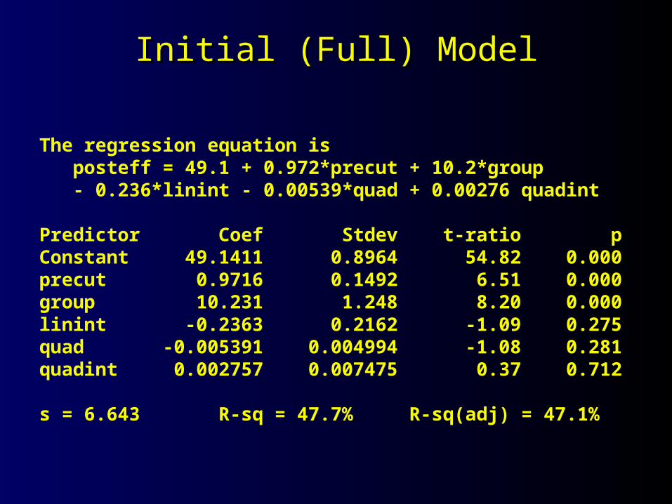
Initial (Full) ModelInitial (Full) Model

The regression equation is posteff = 49.1 + 0.972*precut + 10.2*group - 0.236*linint - 0.00539*quad + 0.00276 quadint

Predictor Coef Stdev t-ratio pConstant 49.1411 0.8964 54.82 0.000precut 0.9716 0.1492 6.51 0.000group 10.231 1.248 8.20 0.000linint -0.2363 0.2162 -1.09 0.275quad -0.005391 0.004994 -1.08 0.281quadint 0.002757 0.007475 0.37 0.712

s = 6.643 R-sq = 47.7% R-sq(adj) = 47.1%

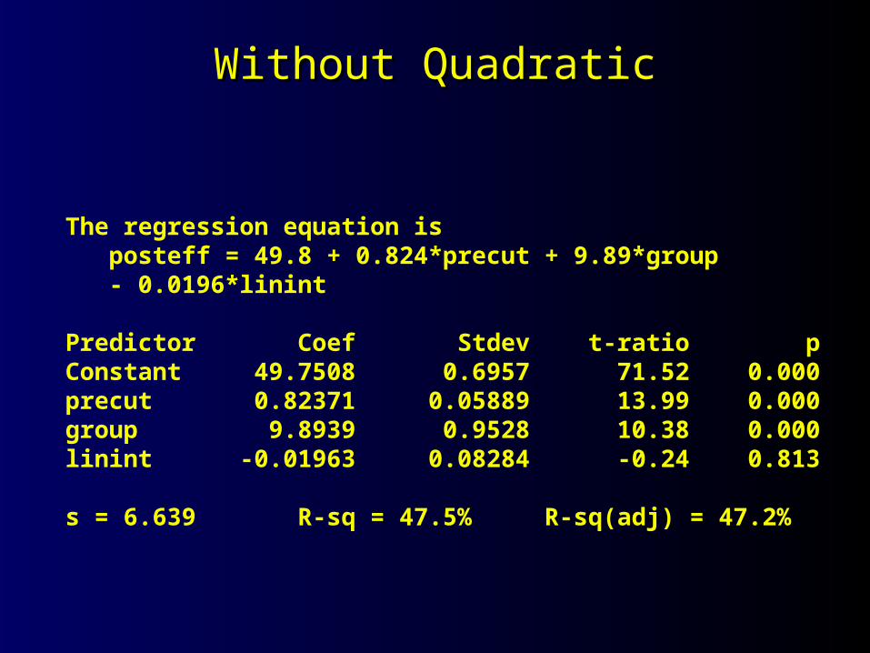
Without QuadraticWithout Quadratic

The regression equation is posteff = 49.8 + 0.824*precut + 9.89*group - 0.0196*linint

Predictor Coef Stdev t-ratio pConstant 49.7508 0.6957 71.52 0.000precut 0.82371 0.05889 13.99 0.000group 9.8939 0.9528 10.38 0.000linint -0.01963 0.08284 -0.24 0.813

s = 6.639 R-sq = 47.5% R-sq(adj) = 47.2%

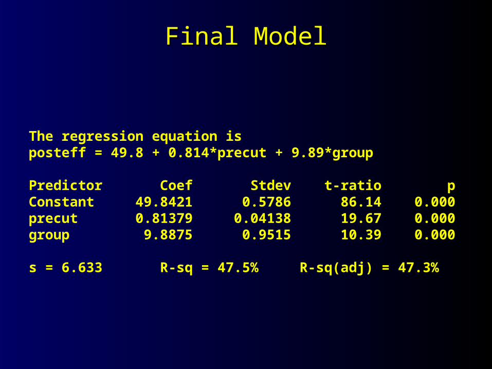
Final ModelFinal Model

The regression equation isposteff = 49.8 + 0.814*precut + 9.89*group

Predictor Coef Stdev t-ratio pConstant 49.8421 0.5786 86.14 0.000precut 0.81379 0.04138 19.67 0.000group 9.8875 0.9515 10.39 0.000

s = 6.633 R-sq = 47.5% R-sq(adj) = 47.3%

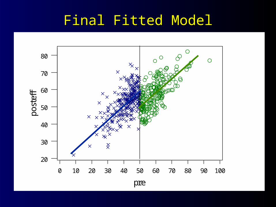
Final Fitted ModelFinal Fitted Model

1009080706050403020100

80

70

60

50

40

30

20

pre

po

ste

ff