Introduction to CFD Analysis - · PDF file2-1 © Fluent Inc. 12/26/2001 Introductory FLUENT Notes FLUENT v6.0 Jan 2002 Fluent User Services Center Introduction to CFD Analysis

© Fluent Inc. 12/26/20012-1

Introductory FLUENT NotesFLUENT v6.0 Jan 2002

Fluent User Services Center

www.fluentusers.com

Introduction to CFD Analysis

© Fluent Inc. 12/26/20012-2



www.fluentusers.com

What is CFD?

Computational Fluid Dynamics (CFD) is the science of predicting fluid flow, heat transfer, mass transfer, chemical reactions, and related phenomena by solving mathematical equations that represent physical laws, using a numerical process.

Conservation of mass, momentum, energy, species, ...The result of CFD analyses is relevant engineering data:

conceptual studies of new designsdetailed product developmenttroubleshootingredesign

CFD analysis complements testing and experimentation.Reduces the total effort required in the laboratory.

© Fluent Inc. 12/26/20012-3



www.fluentusers.com

How does CFD work?

FLUENT solvers are based on thefinite volume method.

Domain is discretized into a finite set of control volumes or cells.General conservation (transport) equation for mass, momentum, energy, etc.,

are discretized into algebraic equations.

All equations are solved to render flow field.

∫∫∫∫ +⋅∇Γ=⋅+∂∂

VAAV

dVSdddVt φφρφρφ AAV

unsteady convection diffusion generation

Eqn.continuity 1

x-mom. uy-mom. venergy h

φ

Fluid region of pipe flow discretized into finite set of control volumes (mesh).

control volume

© Fluent Inc. 12/26/20012-4



www.fluentusers.com

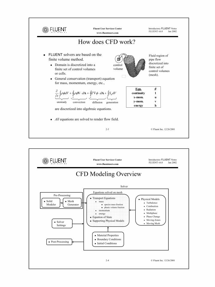
CFD Modeling Overview

Transport Equationsmass

species mass fractionphasic volume fraction

momentumenergy

Equation of StateSupporting Physical Models

Solver

Physical ModelsTurbulenceCombustionRadiationMultiphasePhase ChangeMoving ZonesMoving Mesh

Mesh Generator

Material PropertiesBoundary ConditionsInitial Conditions

Solver Settings

Pre-Processing

Solid Modeler

Post-Processing

Equations solved on mesh

© Fluent Inc. 12/26/20012-5



www.fluentusers.com

CFD Analysis: Basic Steps

Problem Identification and Pre-Processing1. Define your modeling goals.2. Identify the domain you will model.3. Design and create the grid.Solver Execution4. Set up the numerical model.5. Compute and monitor the solution.Post-Processing6. Examine the results.7. Consider revisions to the model.

© Fluent Inc. 12/26/20012-6



www.fluentusers.com

Define Your Modeling Goals

What results are you looking for, and how will they be used?What are your modeling options?

What physical models will need to be included in your analysis?What simplifying assumptions do you have to make?What simplifying assumptions can you make?Do you require a unique modeling capability?

User-defined functions (written in C) in FLUENT 6User-defined subroutines (written in FORTRAN) in FLUENT 4.5

What degree of accuracy is required?How quickly do you need the results?

Problem Identification and Pre-Processing1. Define your modeling goals.2. Identify the domain you will model.3. Design and create the grid.

© Fluent Inc. 12/26/20012-7



www.fluentusers.com

Identify the Domain You Will Model

How will you isolate a piece of the complete physical system?Where will the computational domain begin and end?

Do you have boundary condition information at these boundaries?Can the boundary condition types accommodate that information?Can you extend the domain to a point where reasonable data exists?

Can the problem be simplified to 2D?

Problem Identification and Pre-Processing1. Define your modeling goals.2. Identify the domain you will model.3. Design and create the grid

Gas

Riser

Cyclone

L-valve

Gas Example: Cyclone Separator

© Fluent Inc. 12/26/20012-8



www.fluentusers.com

Design and Create the GridCan you benefit from Mixsim, Icepak, or Airpak?Can you use a quad/hex grid or should you use a tri/tet grid or hybrid grid?

How complex is the geometry and flow?Will you need a non-conformal interface?

What degree of grid resolution is required in each region of the domain?

Is the resolution sufficient for the geometry?Can you predict regions with high gradients?Will you use adaption to add resolution?

Do you have sufficient computer memory?How many cells are required?How many models will be used?

triangle quadrilateral

tetrahedron

pyramid prism/wedge

hexahedron

Problem Identification and Pre-Processing1. Define your modeling goals.2. Identify the domain you will model.3. Design and create the grid.

© Fluent Inc. 12/26/20012-9



www.fluentusers.com

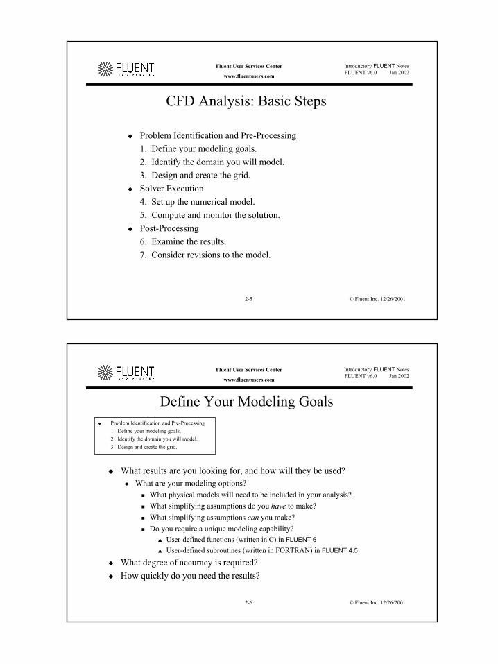
Tri/Tet vs. Quad/Hex Meshes

For simple geometries, quad/hex meshes can provide high-quality solutions with fewer cells than a comparable tri/tet mesh.

Align the gridlines with the flow.

For complex geometries, quad/hex meshes show no numerical advantage, and you can save meshing effort by using a tri/tet mesh.

© Fluent Inc. 12/26/20012-10



www.fluentusers.com

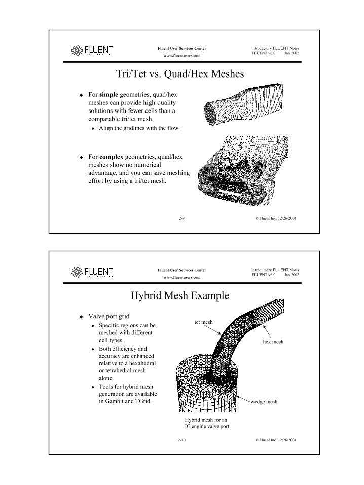
Hybrid Mesh Example

Valve port gridSpecific regions can be meshed with different cell types.Both efficiency and accuracy are enhanced relative to a hexahedral or tetrahedral mesh alone.Tools for hybrid mesh generation are available in Gambit and TGrid.

Hybrid mesh for an IC engine valve port

tet mesh

hex mesh

wedge mesh

© Fluent Inc. 12/26/20012-11



www.fluentusers.com

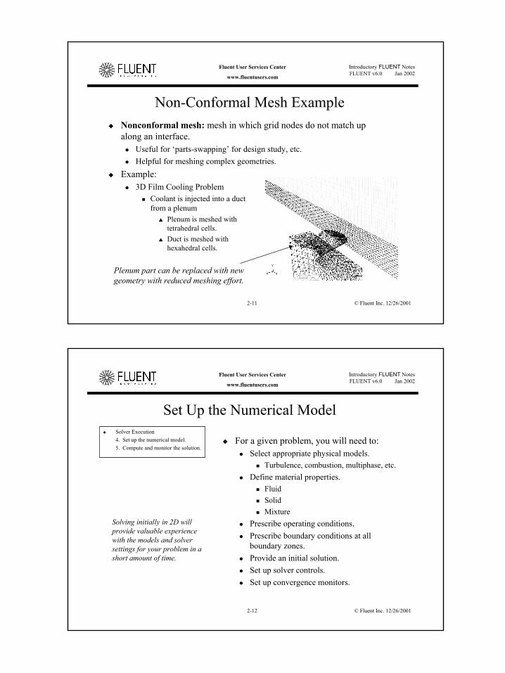
Non-Conformal Mesh ExampleNonconformal mesh: mesh in which grid nodes do not match up along an interface.

Useful for ‘parts-swapping’ for design study, etc.Helpful for meshing complex geometries.

Example:3D Film Cooling Problem

Coolant is injected into a ductfrom a plenum

Plenum is meshed withtetrahedral cells.Duct is meshed withhexahedral cells.

Plenum part can be replaced with new geometry with reduced meshing effort.

© Fluent Inc. 12/26/20012-12



www.fluentusers.com

Set Up the Numerical Model

For a given problem, you will need to:Select appropriate physical models.

Turbulence, combustion, multiphase, etc.Define material properties.

Fluid SolidMixture

Prescribe operating conditions.Prescribe boundary conditions at all boundary zones.Provide an initial solution.Set up solver controls.Set up convergence monitors.

Solver Execution4. Set up the numerical model.5. Compute and monitor the solution.

Solving initially in 2D will provide valuable experience with the models and solver settings for your problem in a short amount of time.

© Fluent Inc. 12/26/20012-13



www.fluentusers.com

Compute the SolutionThe discretized conservation equations are solved iteratively.

A number of iterations are usually required to reach a converged solution.

Convergence is reached when:Changes in solution variables from one iteration to the next are negligible.

Residuals provide a mechanism to help monitor this trend.

Overall property conservation is achieved.The accuracy of a converged solution is dependent upon:

Appropriateness and accuracy of physical models.Grid resolution and independenceProblem setup

Solver Execution4. Set up the numerical model.5. Compute and monitor the solution.

A converged and grid-independent solution on a well-posed problem will provide useful engineering results!

© Fluent Inc. 12/26/20012-14



www.fluentusers.com

Examine the ResultsExamine the results to review solution and extract useful data.

Visualization Tools can be used to answer such questions as:

What is the overall flow pattern?Is there separation?Where do shocks, shear layers, etc. form?Are key flow features being resolved?

Numerical Reporting Tools can be used to calculate quantitative results:

Forces and MomentsAverage heat transfer coefficientsSurface and Volume integrated quantitiesFlux Balances

Post-Processing6. Examine the results.7. Consider revisions to the model.

Examine results to ensure property conservation and correct physical behavior. High residuals may be attributable to only a few cells of poor quality.

© Fluent Inc. 12/26/20012-15



www.fluentusers.com

Consider Revisions to the ModelAre physical models appropriate?

Is flow turbulent?Is flow unsteady?Are there compressibility effects?Are there 3D effects?

Are boundary conditions correct?Is the computational domain large enough?Are boundary conditions appropriate?Are boundary values reasonable?

Is grid adequate?Can grid be adapted to improve results?Does solution change significantly with adaption, or is the solution grid independent?Does boundary resolution need to be improved?

Post-Processing6. Examine the results.7. Consider revisions to the model.

© Fluent Inc. 12/26/20012-16



www.fluentusers.com

FLUENT DEMO

Startup Gambit (Pre-processing)load databasedefine boundary zonesexport mesh

Startup Fluent (Solver Execution)GUIProblem SetupSolve

Post-ProcessingOnline Documentation

© Fluent Inc. 1/29/023-1



www.fluentusers .com

Solver Basics

© Fluent Inc. 1/29/023-2




Solver Execution

u Solver Execution:l Menu is laid out such that order of

operation is generally left to right.n Import and scale mesh file.n Select physical models.n Define material properties.n Prescribe operating conditions.n Prescribe boundary conditions.n Provide an initial solution.n Set solver controls.n Set up convergence monitors.n Compute and monitor solution.

l Post-Processingn Feedback into Solvern Engineering Analysis

© Fluent Inc. 1/29/023-4




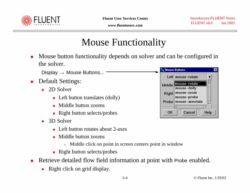
Mouse Functionalityu Mouse button functionality depends on solver and can be configured in

the solver.Display → Mouse Buttons...

u Default Settings:l 2D Solver

n Left button translates (dolly)n Middle button zoomsn Right button selects/probes

l 3D Solvern Left button rotates about 2-axesn Middle button zooms

s Middle click on point in screen centers point in window

n Right button selects/probes

u Retrieve detailed flow field information at point with Probe enabled.l Right click on grid display.

© Fluent Inc. 1/29/023-5




Reading Mesh: Mesh Components

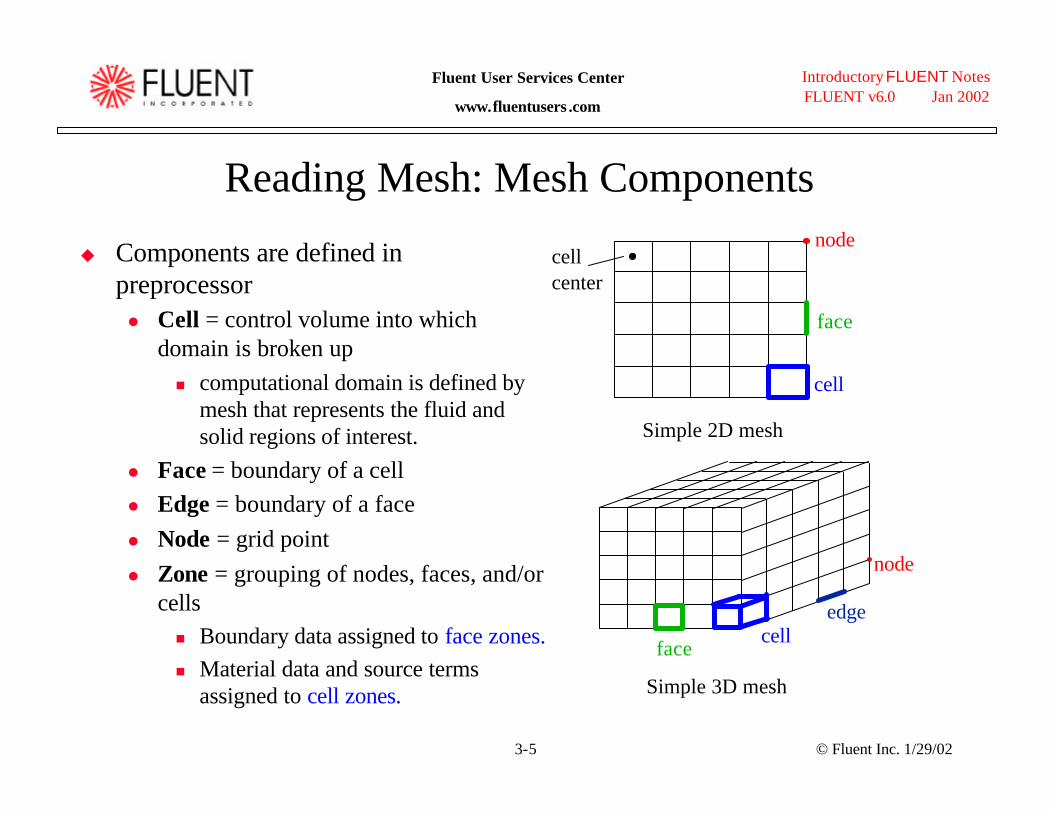
u Components are defined in preprocessorl Cell = control volume into which

domain is broken upn computational domain is defined by

mesh that represents the fluid and solid regions of interest.

l Face = boundary of a celll Edge = boundary of a facel Node = grid pointl Zone = grouping of nodes, faces, and/or

cellsn Boundary data assigned to face zones.n Material data and source terms

assigned to cell zones.

facecell

node

edge

Simple 2D mesh

Simple 3D mesh

node

face

cell

cell center

© Fluent Inc. 1/29/023-7




Scaling Mesh and Units

u All physical dimensions initially assumed to be in meters.l Scale grid accordingly.

u Other quantities can also be scaled independent of other units used.l Fluent defaults to SI units.

© Fluent Inc. 1/29/023-8




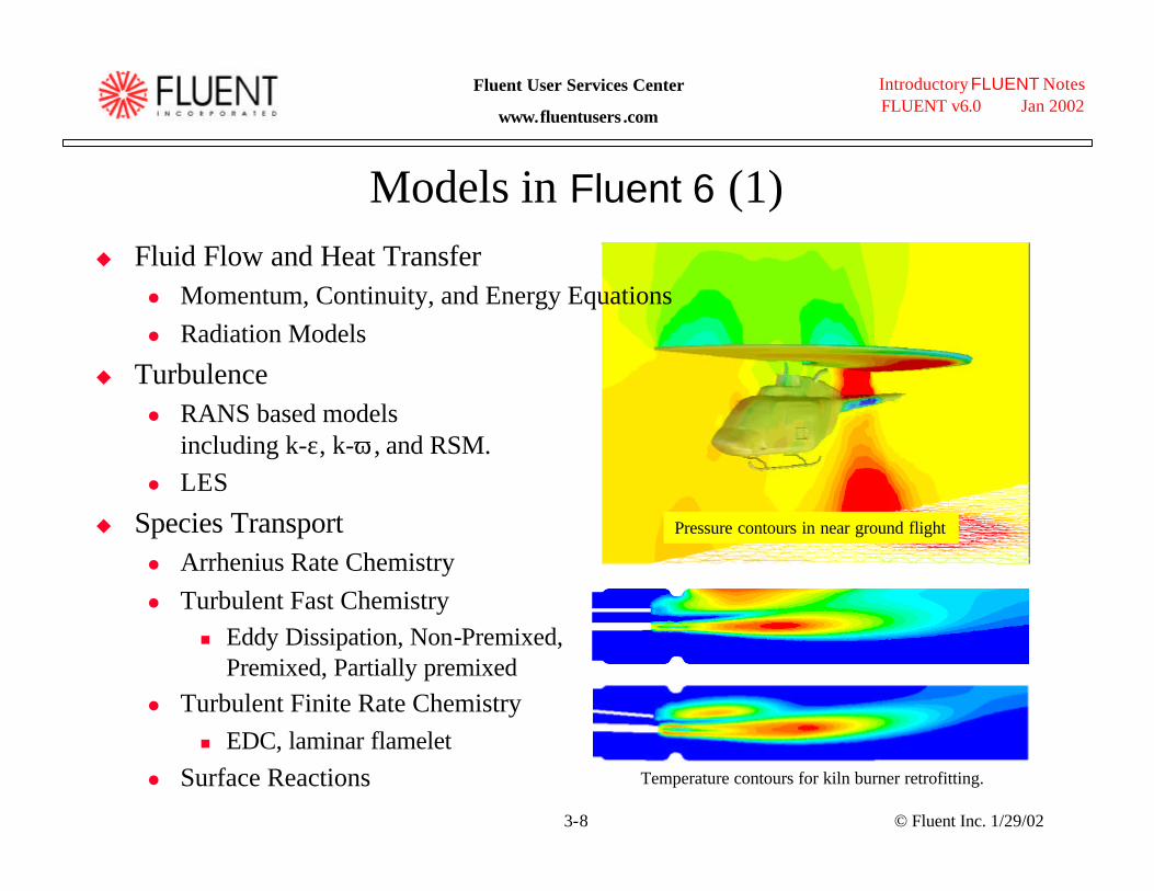
u Fluid Flow and Heat Transferl Momentum, Continuity, and Energy Equationsl Radiation Models

u Turbulencel RANS based models

including k-ε, k-ω, and RSM.l LES

u Species Transportl Arrhenius Rate Chemistryl Turbulent Fast Chemistry

n Eddy Dissipation, Non-Premixed, Premixed, Partially premixed

l Turbulent Finite Rate Chemistryn EDC, laminar flamelet

l Surface Reactions

Models in Fluent 6 (1)

Pressure contours in near ground flight

Temperature contours for kiln burner retrofitting.

© Fluent Inc. 1/29/023-9




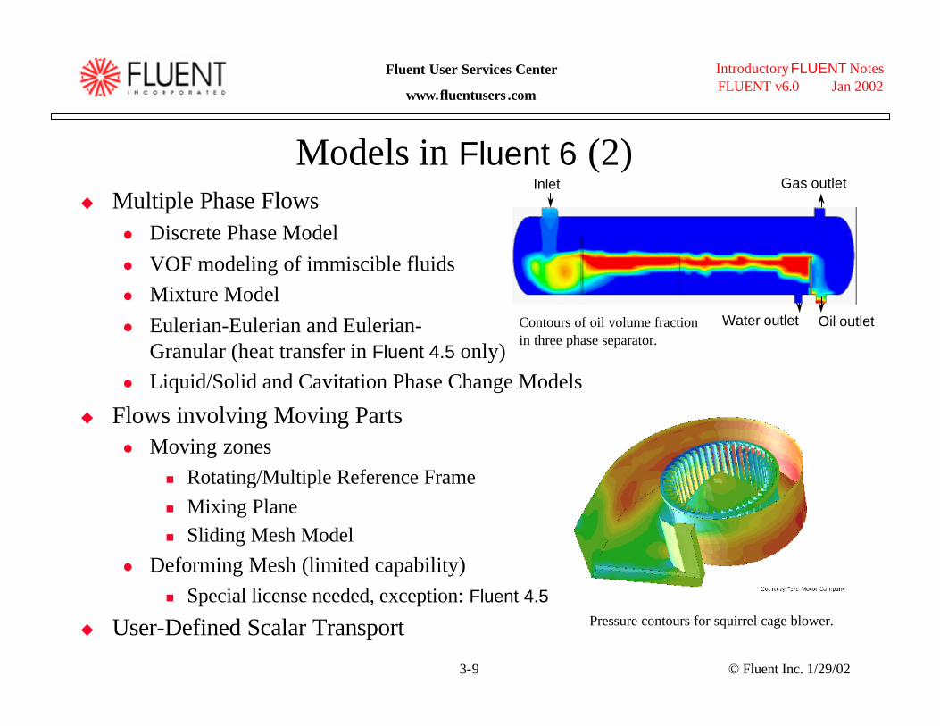
u Multiple Phase Flowsl Discrete Phase Modell VOF modeling of immiscible fluidsl Mixture Modell Eulerian-Eulerian and Eulerian-

Granular (heat transfer in Fluent 4.5 only)l Liquid/Solid and Cavitation Phase Change Models

u Flows involving Moving Partsl Moving zones

n Rotating/Multiple Reference Framen Mixing Planen Sliding Mesh Model

l Deforming Mesh (limited capability)n Special license needed, exception: Fluent 4.5

u User-Defined Scalar Transport

Models in Fluent 6 (2)Gas outlet

Oil outlet

Inlet

Water outletContours of oil volume fraction in three phase separator.

Pressure contours for squirrel cage blower.

© Fluent Inc. 1/29/023-10




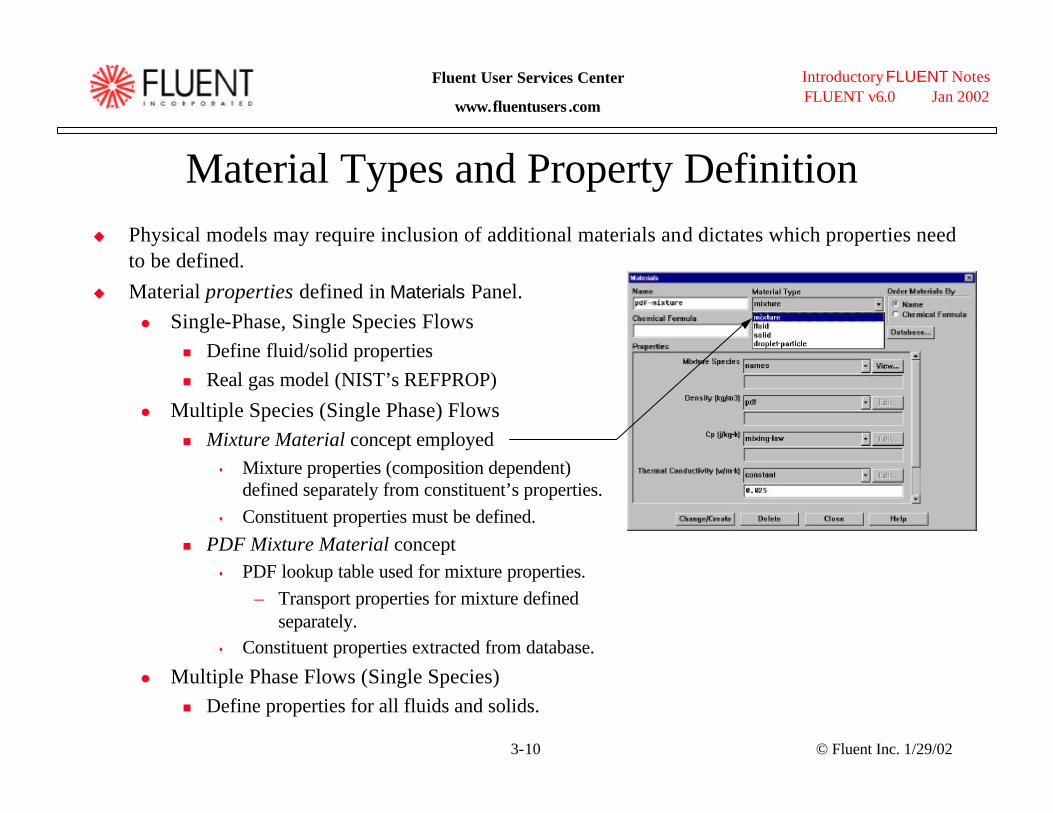
Material Types and Property Definitionu Physical models may require inclusion of additional materials and dictates which properties need

to be defined.u Material properties defined in Materials Panel.

l Single-Phase, Single Species Flowsn Define fluid/solid propertiesn Real gas model (NIST’s REFPROP)

l Multiple Species (Single Phase) Flowsn Mixture Material concept employed

s Mixture properties (composition dependent) defined separately from constituent’s properties.

s Constituent properties must be defined.n PDF Mixture Material concept

s PDF lookup table used for mixture properties.– Transport properties for mixture defined

separately.s Constituent properties extracted from database.

l Multiple Phase Flows (Single Species)n Define properties for all fluids and solids.

© Fluent Inc. 1/29/023-11




Fluid Density

u For ρ = constant, incompressible flow:l Select constant in Define → Materials...

u For incompressible flow: l ρ = poperating/RT

n Use incompressible-ideal-gas

n Set poperating close to mean pressure in problem.

u For compressible flow use ideal-gas:l ρ = pabsolute/RT

n For low Mach number flows, set poperating close to mean pressure in problem to avoid round-off errors.

n Use Floating Operating Pressure for unsteady flows with large, gradual changes in absolute pressure (seg. only).

u Density can also be defined as a function of Temperaturel polynomial or piecewise-polynomial

l boussinesq model discussed in heat transfer lecture.

u Density can also be defined using UDF- not to be function of pressure!

© Fluent Inc. 1/29/023-13




Solver Execution: Other Lectures...

u Physical models discussed on Day 2.

© Fluent Inc. 1/29/023-14




Post-Processingu Many post-processing tools are available.u Post-Processing functions typically operate on surfaces.

l Surfaces are automatically created from zones.l Additional surfaces can be created.

u Example: an Iso-Surface of constant grid coordinate can be created for viewing data within a plane.

© Fluent Inc. 1/29/023-15




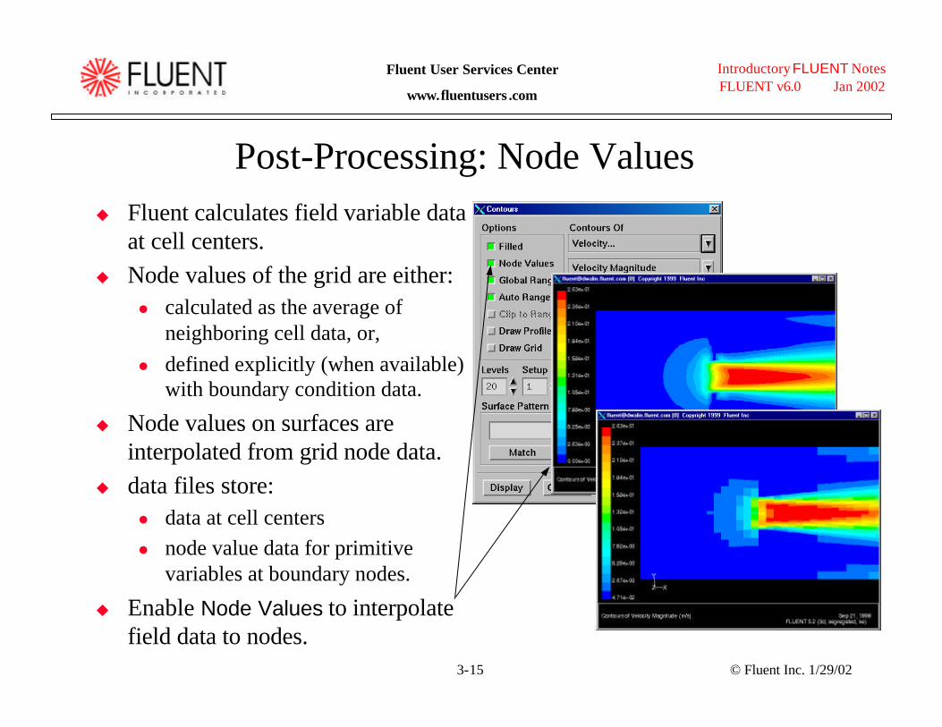
Post-Processing: Node Valuesu Fluent calculates field variable data

at cell centers.u Node values of the grid are either:

l calculated as the average of neighboring cell data, or,

l defined explicitly (when available) with boundary condition data.

u Node values on surfaces are interpolated from grid node data.

u data files store:l data at cell centersl node value data for primitive

variables at boundary nodes.

u Enable Node Values to interpolate field data to nodes.

© Fluent Inc. 1/29/023-16




Reportsu Flux Reports

l Net flux is calculated.l Total Heat Transfer Rate

includes radiation.

u Surface Integralsl slightly less accurate on

user-generated surfaces due to interpolation error.

u Volume Integrals

Examples:

© Fluent Inc. 1/29/023-17




Solver Enhancements: Grid Adaptionu Grid adaption adds more cells where needed to

resolve the flow field without pre-processor.u Fluent adapts on cells listed in register.

l Registers can be defined based on:n Gradients of flow or user-defined variablesn Iso-values of flow or user-defined variablesn All cells on a boundaryn All cells in a regionn Cell volumes or volume changesn y+ in cells adjacent to walls

l To assist adaption process, you can:n Combine adaption registersn Draw contours of adaption functionn Display cells marked for adaptionn Limit adaption based on cell size

and number of cells:

© Fluent Inc. 1/29/023-18




Adaption Example: 2D Planar Shell

2D planar shell - initial grid

u Adapt grid in regions of high pressure gradient to better resolve pressure jump across the shock.

2D planar shell - contours of pressure initial grid

© Fluent Inc. 1/29/023-19




Adaption Example: Final Grid and Solution

2D planar shell - contours of pressure final grid

2D planar shell - final grid

© Fluent Inc. 1/29/024-1




Boundary Conditions

© Fluent Inc. 1/29/024-2




Defining Boundary Conditions

u To define a problem that results in a unique solution, you must specify information on the dependent (flow) variables at the domain boundaries.l Specifying fluxes of mass, momentum, energy, etc. into domain.

u Defining boundary conditions involves:l identifying the location of the boundaries (e.g., inlets, walls, symmetry)l supplying information at the boundaries

u The data required at a boundary depends upon the boundary condition type and the physical models employed.

u You must be aware of the information that is required of the boundary condition and locate the boundaries where the information on the flow variables are known or can be reasonably approximated.l Poorly defined boundary conditions can have a significant impact on your

solution.

© Fluent Inc. 1/29/024-3




Fuel

Air

Combustor Wall

Manifold box

1

1

23

Nozzle

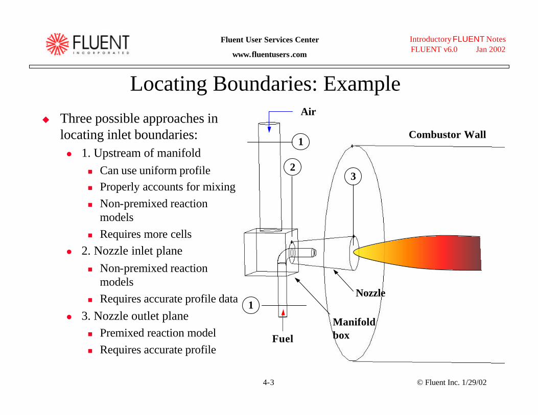
Locating Boundaries: Exampleu Three possible approaches in

locating inlet boundaries:l 1. Upstream of manifold

n Can use uniform profilen Properly accounts for mixingn Non-premixed reaction

modelsn Requires more cells

l 2. Nozzle inlet planen Non-premixed reaction

modelsn Requires accurate profile data

l 3. Nozzle outlet planen Premixed reaction modeln Requires accurate profile

© Fluent Inc. 1/29/024-4




General Guidelines

u General guidelines:l If possible, select boundary

location and shape such that flow either goes in or out.n Not necessary, but will typically

observe better convergence.l Should not observe large

gradients in direction normal to boundary.n Indicates incorrect set-up.

l Minimize grid skewness near boundary.n Introduces error early in

calculation.21

Upper pressure boundary modified to ensure that flow always enters domain.

© Fluent Inc. 1/29/024-5




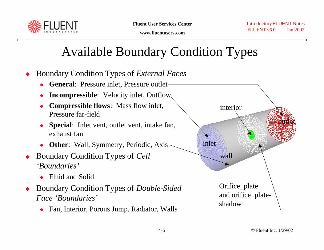
Available Boundary Condition Types

u Boundary Condition Types of External Facesl General: Pressure inlet, Pressure outletl Incompressible: Velocity inlet, Outflowl Compressible flows: Mass flow inlet,

Pressure far-fieldl Special: Inlet vent, outlet vent, intake fan,

exhaust fanl Other: Wall, Symmetry, Periodic, Axis

u Boundary Condition Types of Cell ‘Boundaries’l Fluid and Solid

u Boundary Condition Types of Double-Sided Face ‘Boundaries’l Fan, Interior, Porous Jump, Radiator, Walls

inlet

outlet

wall

interior

Orifice_plate and orifice_plate-shadow

© Fluent Inc. 1/29/024-6




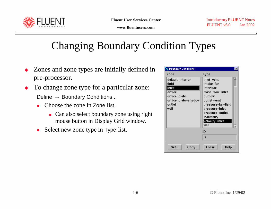
Changing Boundary Condition Types

u Zones and zone types are initially defined in pre-processor.

u To change zone type for a particular zone:Define → Boundary Conditions...

l Choose the zone in Zone list.n Can also select boundary zone using right

mouse button in Display Grid window.l Select new zone type in Type list.

© Fluent Inc. 1/29/024-7




Setting Boundary Condition Datau Explicitly assign data in BC panels.

l To set boundary conditions for particular zone:n Choose the zone in Zone list.n Click Set... button

l Boundary condition data can be copied from one zone to another.

u Boundary condition data can be stored and retrieved from file.l file → write-bc and file → read-bc

u Boundary conditions can also be defined by UDFs and Profiles.

u Profiles can be generated by:l Writing a profile from another CFD simulationl Creating an appropriately formatted text file

with boundary condition data.

© Fluent Inc. 1/29/024-8




Velocity Inlet

u Specify Velocity by:l Magnitude, Normal to Boundaryl Componentsl Magnitude and Direction

u Velocity profile is uniform by defaultu Intended for incompressible flows.

l Static pressure adjusts to accommodate prescribed velocity distribution.

l Total (stagnation) properties of flow also varies.l Using in compressible flows can lead to non-physical results.

u Can be used as an outlet by specifying negative velocity.l You must ensure that mass conservation is satisfied if multiple inlets are used.

© Fluent Inc. 1/29/024-9




Pressure Inlet (1)u Specify:

l Total Gauge Pressuren Defines energy to drive flow.n Doubles as back pressure (static gauge)

for cases where back flow occurs.s Direction of back flow determined

from interior solution.

l Static Gauge Pressuren Static pressure where flow is locally

supersonic; ignored if subsonicn Will be used if flow field is initialized

from this boundary.l Total Temperature

n Used as static temperature for incompressible flow.

l Inlet Flow Direction

21(1 )

2total statick

T T M−

= +

2 /( 1), ,

1(1 )

2k k

total abs static absk

p p M −−= +

2

21

vpp statictotal ρ+=Incompressible flows:

Compressible flows:

© Fluent Inc. 1/29/024-10




Pressure Inlet (2)

u Note: Gauge pressure inputs are required.l

l Operating pressure input is set under: Define → Operating Conditions

u Suitable for compressible and incompressible flows.l Pressure inlet boundary is treated as loss-free transition from stagnation to

inlet conditions.l Fluent calculates static pressure and velocity at inletl Mass flux through boundary varies depending on interior solution and

specified flow direction.

u Can be used as a “free” boundary in an external or unconfined flow.

operatinggaugeabsolute ppp +=

© Fluent Inc. 1/29/024-12




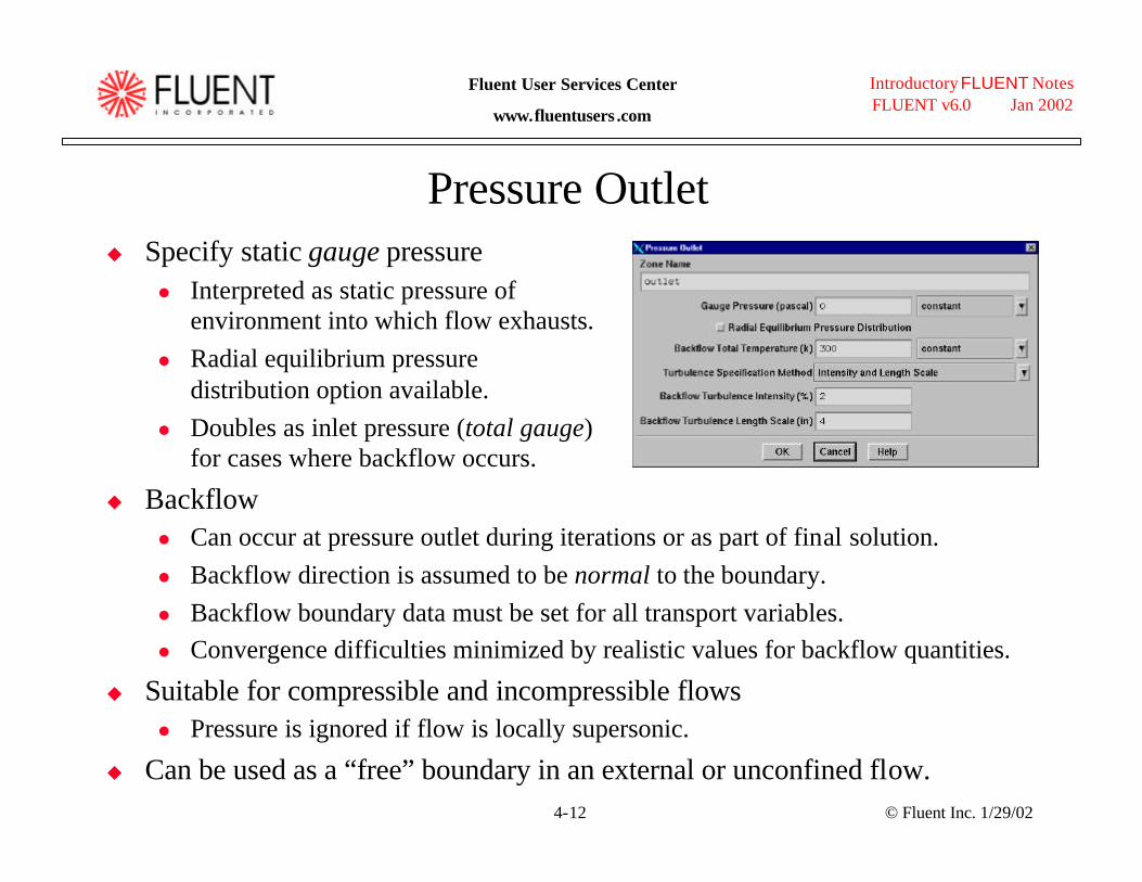
Pressure Outletu Specify static gauge pressure

l Interpreted as static pressure of environment into which flow exhausts.

l Radial equilibrium pressuredistribution option available.

l Doubles as inlet pressure (total gauge)for cases where backflow occurs.

u Backflowl Can occur at pressure outlet during iterations or as part of final solution.l Backflow direction is assumed to be normal to the boundary.l Backflow boundary data must be set for all transport variables.l Convergence difficulties minimized by realistic values for backflow quantities.

u Suitable for compressible and incompressible flowsl Pressure is ignored if flow is locally supersonic.

u Can be used as a “free” boundary in an external or unconfined flow.

© Fluent Inc. 1/29/024-13




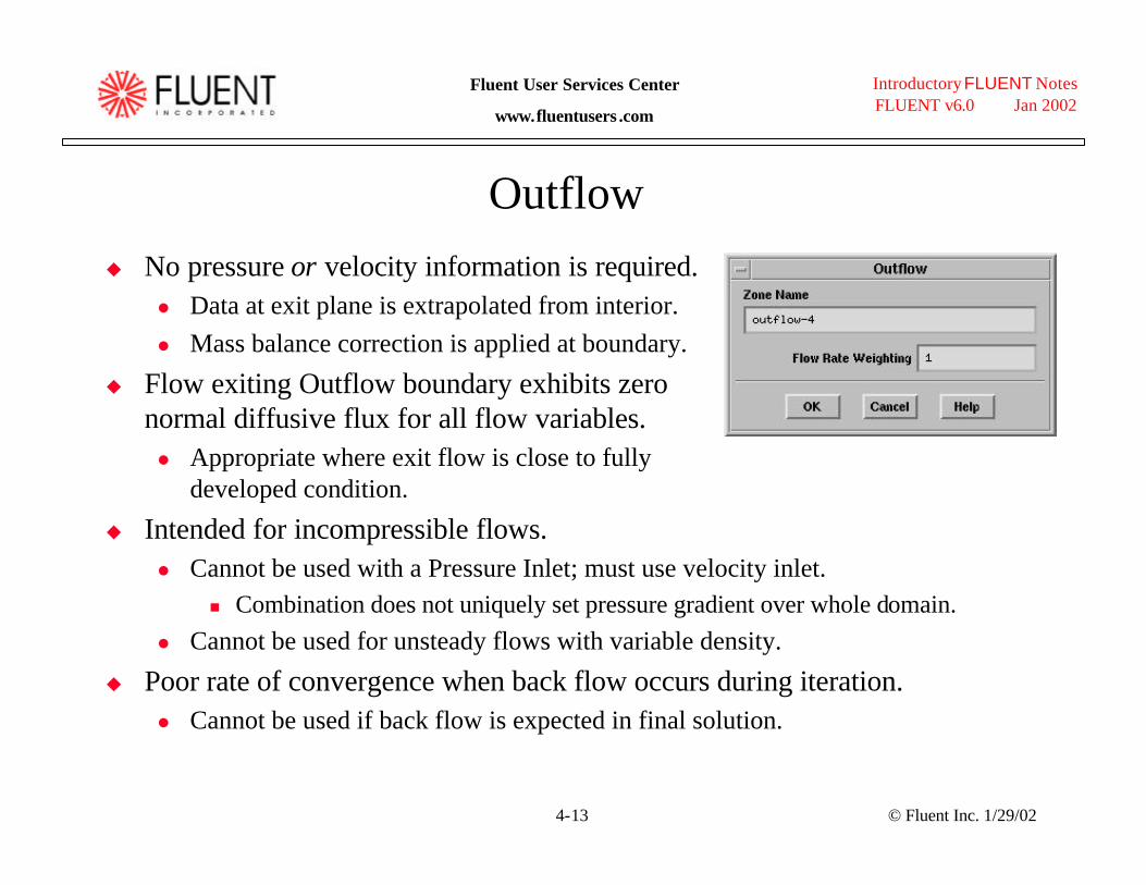
Outflowu No pressure or velocity information is required.

l Data at exit plane is extrapolated from interior.l Mass balance correction is applied at boundary.

u Flow exiting Outflow boundary exhibits zero normal diffusive flux for all flow variables.l Appropriate where exit flow is close to fully

developed condition.

u Intended for incompressible flows.l Cannot be used with a Pressure Inlet; must use velocity inlet.

n Combination does not uniquely set pressure gradient over whole domain. l Cannot be used for unsteady flows with variable density.

u Poor rate of convergence when back flow occurs during iteration.l Cannot be used if back flow is expected in final solution.

© Fluent Inc. 1/29/024-14




Modeling Multiple Exitsu Flows with multiple exits can be modeled using Pressure Outlet or

Outflow boundaries.l Pressure Outlets

l Outflow:n Mass flow rate fraction determined from Flow Rate Weighting by:

s mi=FRW i/ΣFRW i where 0 < FRW < 1.

s FRW set to 1 by default implying equal flow rates

n static pressure varies among exits to accommodate flow distribution.

pressure-inlet (p0,T0) pressure-outlet (ps)2

velocity-inlet (v,T0)pressure-outlet (ps)1

or

FRW2

velocity inlet

FRW1

© Fluent Inc. 1/29/024-16




Wall Boundaries

u Used to bound fluid and solid regions.u In viscous flows, no-slip condition

enforced at walls:l Tangential fluid velocity equal

to wall velocity.l Normal velocity component = 0l Shear stress can also be specified.

u Thermal boundary conditions:l several types availablel Wall material and thickness can be defined for 1-D or shell conduction heat transfer

calculations.

u Wall roughness can be defined for turbulent flows.l Wall shear stress and heat transfer based on local flow field.

u Translational or rotational velocity can be assigned to wall.

© Fluent Inc. 1/29/024-19




Cell Zones: Fluidu Fluid zone = group of cells for

which all active equations are solved.

u Fluid material input required.l Single species, phase.

u Optional inputs allow setting of source terms:l mass, momentum, energy, etc.

u Define fluid zone as laminar flow region if modeling transitional flow.

u Can define zone as porous media.u Define axis of rotation for rotationally periodic flows.u Can define motion for fluid zone.

© Fluent Inc. 1/29/024-21




Cell Zones: Solidu “Solid” zone = group of cells for which only

heat conduction problem solved.l No flow equations solvedl Material being treated as solid may actually

be fluid, but it is assumed that no convection takes place.

u Only required input is material typel So appropriate material properties used.

u Optional inputs allow you to set volumetric heat generation rate (heat source).

u Need to specify rotation axis if rotationally periodic boundaries adjacent to solid zone.

u Can define motion for solid zone

© Fluent Inc. 1/29/024-22




Internal Face Boundaries

u Defined on cell facesl Do not have finite thicknessl Provide means of introducing step change in flow properties.

u Used to implement physical models representing:l Fansl Radiatorsl Porous jump

n Preferable over porous media- exhibits better convergence behavior.l Interior wall

© Fluent Inc. 1/29/024-23




Summary

u Zones are used to assign boundary conditions.u Wide range of boundary conditions permit flow to enter and exit

solution domain.u Wall boundary conditions used to bound fluid and solid regions.u Repeating boundaries used to reduce computational effort.u Internal cell zones used to specify fluid, solid, and porous regions.u Internal face boundaries provide way to introduce step change in flow

properties.

© Fluent Inc. 1/29/025-1




Solver Settings

© Fluent Inc. 1/29/025-2




Outlineu Using the Solver

l Setting Solver Parametersl Convergence

n Definitionn Monitoringn Stabilityn Accelerating Convergence

l Accuracyn Grid Independencen Adaption

u Appendix: Backgroundl Finite Volume Methodl Explicit vs. Implicitl Segregated vs. Coupledl Transient Solutions

© Fluent Inc. 1/29/025-3




Modify solution parameters or grid

NoYes

No

Set the solution parameters

Initialize the solution

Enable the solution monitors of interest

Calculate a solution

Check for convergence

Check for accuracy

Stop

Yes

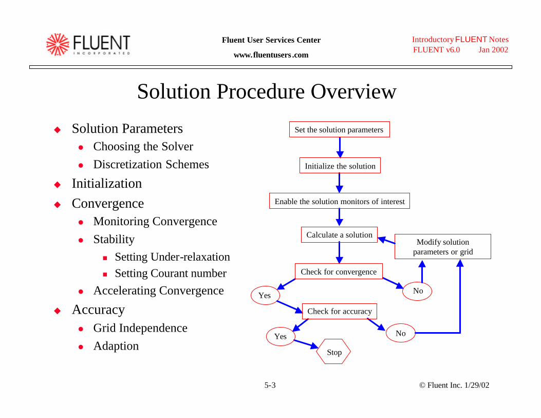
Solution Procedure Overview

u Solution Parametersl Choosing the Solverl Discretization Schemes

u Initializationu Convergence

l Monitoring Convergencel Stability

n Setting Under-relaxationn Setting Courant number

l Accelerating Convergence

u Accuracyl Grid Independencel Adaption

© Fluent Inc. 1/29/025-4




Choosing a Solveru Choices are Coupled-Implicit, Coupled-Explicit, or Segregated (Implicit)u The Coupled solvers are recommended if a strong inter-dependence exists

between density, energy, momentum, and/or species.l e.g., high speed compressible flow or finite-rate reaction modeled flows.l In general, the Coupled-Implicit solver is recommended over the coupled-explicit

solver.n Time required: Implicit solver runs roughly twice as fast.n Memory required: Implicit solver requires roughly twice as much memory as coupled-

explicit or segregated-implicit solvers!

l The Coupled-Explicit solver should only be used for unsteady flows when the characteristic time scale of problem is on same order as that of the acoustics.n e.g., tracking transient shock wave

u The Segregated (implicit) solver is preferred in all other cases.l Lower memory requirements than coupled-implicit solver.l Segregated approach provides flexibility in solution procedure.

© Fluent Inc. 1/29/025-8




Initializationu Iterative procedure requires that all solution variables be initialized

before calculating a solution.Solve → Initialize → Initialize...l Realistic ‘guesses’ improves solution stability and accelerates convergence.l In some cases, correct initial guess is required:

n Example: high temperature region to initiate chemical reaction.

u “Patch” values for individualvariables in certain regions.Solve → Initialize → Patch...l Free jet flows

(patch high velocity for jet)l Combustion problems

(patch high temperaturefor ignition)

© Fluent Inc. 1/29/025-10




Convergenceu At convergence:

l All discrete conservation equations (momentum, energy, etc.) areobeyed in all cells to a specified tolerance.

l Solution no longer changes with more iterations.l Overall mass, momentum, energy, and scalar balances are obtained.

u Monitoring convergence with residuals:l Generally, a decrease in residuals by 3 orders of magnitude indicates at

least qualitative convergence. n Major flow features established.

l Scaled energy residual must decrease to 10-6 for segregated solver.l Scaled species residual may need to decrease to 10-5 to achieve species

balance.

u Monitoring quantitative convergence:l Monitor other variables for changes.l Ensure that property conservation is satisfied.

© Fluent Inc. 1/29/025-11




Convergence Monitors: Residualsu Residual plots show when the residual values have reached the

specified tolerance.Solve → Monitors → Residual...

All equations converged.

10-3

10-6

© Fluent Inc. 1/29/025-12




Convergence Monitors: Forces/Surfacesu In addition to residuals, you can also monitor:

l Lift, drag, or momentSolve → Monitors → Force...

l Variables or functions (e.g., surface integrals)at a boundary or any defined surface: Solve → Monitors → Surface...

© Fluent Inc. 1/29/025-13




Checking for Property Conservation

u In addition to monitoring residual and variable histories, you should also check for overall heat and mass balances.l At a minimum, the net imbalance should be less than 1% of smallest flux

through domain boundary.Report → Fluxes...

© Fluent Inc. 1/29/025-14




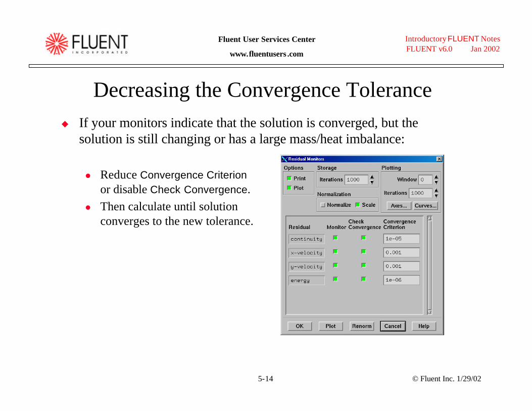
Decreasing the Convergence Toleranceu If your monitors indicate that the solution is converged, but the

solution is still changing or has a large mass/heat imbalance:

l Reduce Convergence Criterionor disable Check Convergence.

l Then calculate until solutionconverges to the new tolerance.

© Fluent Inc. 1/29/025-15




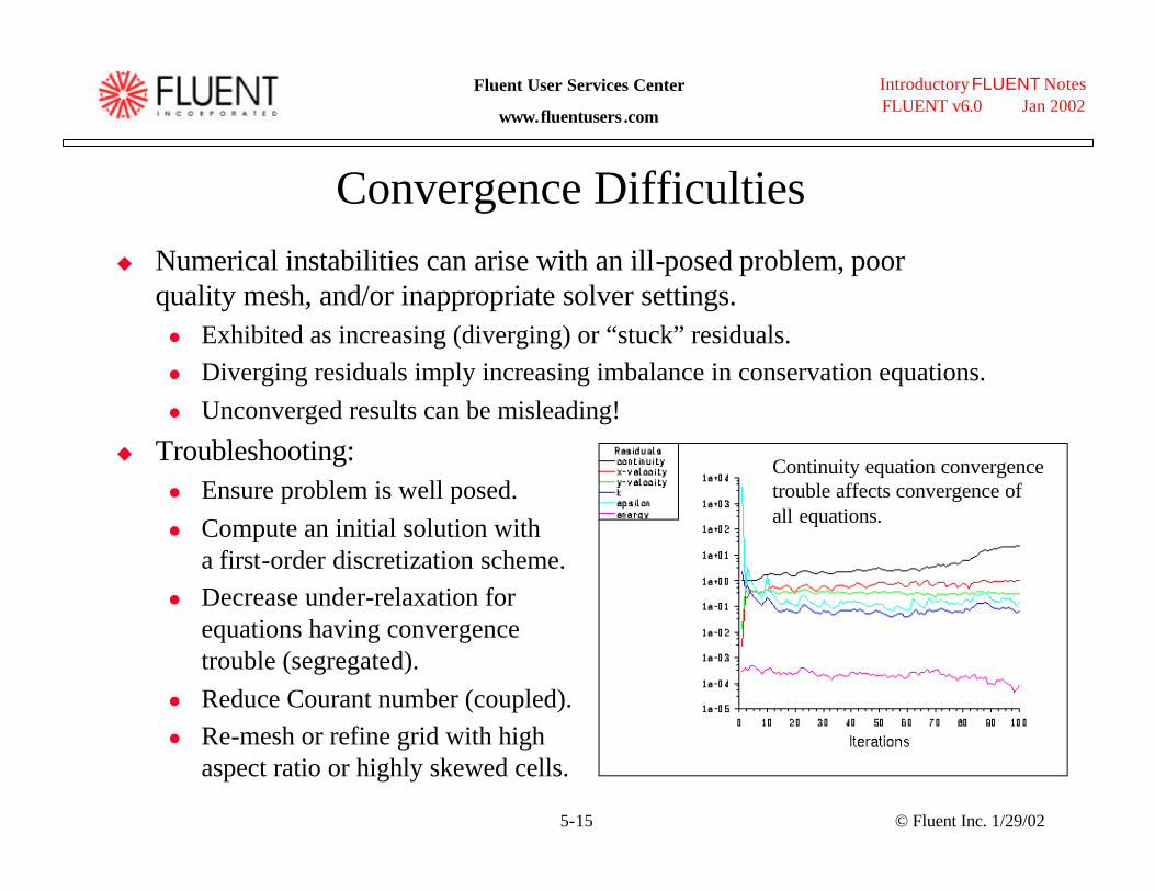
Convergence Difficultiesu Numerical instabilities can arise with an ill-posed problem, poor

quality mesh, and/or inappropriate solver settings.l Exhibited as increasing (diverging) or “stuck” residuals.l Diverging residuals imply increasing imbalance in conservation equations.l Unconverged results can be misleading!

u Troubleshooting:l Ensure problem is well posed.l Compute an initial solution with

a first-order discretization scheme.l Decrease under-relaxation for

equations having convergence trouble (segregated).

l Reduce Courant number (coupled).l Re-mesh or refine grid with high

aspect ratio or highly skewed cells.

Continuity equation convergencetrouble affects convergence ofall equations.

© Fluent Inc. 1/29/025-16




Modifying Under-relaxation Factors

u Under-relaxation factor, α, is included to stabilize the iterative process for the segregated solver.

u Use default under-relaxation factors to start a calculation.

Solve → Controls → Solution...

u Decreasing under-relaxation for momentum often aids convergence.l Default settings are aggressive but

suitable for wide range of problems.l ‘Appropriate’ settings best learned

from experience.

poldpp φαφφ ∆+= ,

u For coupled solvers, under-relaxation factors for equations outside coupled set are modified as in segregated solver.

© Fluent Inc. 1/29/025-17




Modifying the Courant Numberu Courant number defines a ‘time

step’ size for steady-state problems.l A transient term is included in the

coupled solver even for steady state problems.

u For coupled-explicit solver:l Stability constraints impose a

maximum limit on Courant number.n Cannot be greater than 2.

s Default value is 1.

n Reduce Courant number when having difficulty converging.

ux

t∆

=∆)CFL(

u For coupled-implicit solver:l Courant number is not limited by stability constraints.

n Default is set to 5.

© Fluent Inc. 1/29/025-18




Accelerating Convergence

u Convergence can be accelerated by:l Supplying good initial conditions

n Starting from a previous solution.l Increasing under-relaxation factors or Courant number

n Excessively high values can lead to instabilities.n Recommend saving case and data files before continuing iterations.

l Controlling multigrid solver settings.n Default settings define robust Multigrid solver and typically do not need

to be changed.

© Fluent Inc. 1/29/025-21




Accuracy

u A converged solution is not necessarily an accurate one.l Solve using 2nd order discretization.l Ensure that solution is grid-independent.

n Use adaption to modify grid.

u If flow features do not seem reasonable:l Reconsider physical models and boundary conditions.l Examine grid and re-mesh.

© Fluent Inc. 1/29/025-22




Mesh Quality and Solution Accuracyu Numerical errors are associated with calculation of cell gradients and cell

face interpolations.u These errors can be contained:

l Use higher order discretization schemes.l Attempt to align grid with flow.l Refine the mesh.

n Sufficient mesh density is necessary to resolve salient features of flow.s Interpolation errors decrease with decreasing cell size.

n Minimize variations in cell size.s Truncation error is minimized in a uniform mesh.s Fluent provides capability to adapt mesh based on cell size variation.

n Minimize cell skewness and aspect ratio.s In general, avoid aspect ratios higher than 5:1 (higher ratios allowed in b.l.).s Optimal quad/hex cells have bounded angles of 90 degreess Optimal tri/tet cells are equilateral.

© Fluent Inc. 1/29/025-23




Determining Grid Independenceu When solution no longer changes with further grid refinement, you

have a “grid-independent” solution.u Procedure:

l Obtain new grid:n Adapt

s Save original mesh before adapting.– If you know where large gradients are expected, concentrate the

original grid in that region, e.g., boundary layer. s Adapt grid.

– Data from original grid is automatically interpolated to finer grid.

n file → write-bc and file → read-bc facilitates set up of new problem

n file → reread-grid and File → Interpolate...

l Continue calculation to convergence.l Compare results obtained w/different grids.l Repeat procedure if necessary.

© Fluent Inc. 1/29/025-24




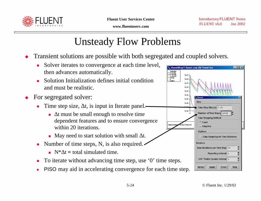
Unsteady Flow Problems u Transient solutions are possible with both segregated and coupled solvers.

l Solver iterates to convergence at each time level, then advances automatically.

l Solution Initialization defines initial condition and must be realistic.

u For segregated solver:l Time step size, ∆t, is input in Iterate panel.

n ∆t must be small enough to resolve time dependent features and to ensure convergence within 20 iterations.

n May need to start solution with small ∆t.l Number of time steps, N, is also required.

n N*∆t = total simulated time.l To iterate without advancing time step, use ‘0’ time steps.l PISO may aid in accelerating convergence for each time step.

© Fluent Inc. 1/29/025-26




Summary

u Solution procedure for the segregated and coupled solvers is the same:l Calculate until you get a converged solution.l Obtain second-order solution (recommended).l Refine grid and recalculate until grid-independent solution is obtained.

u All solvers provide tools for judging and improving convergence and ensuring stability.

u All solvers provide tools for checking and improving accuracy.u Solution accuracy will depend on the appropriateness of the physical

models that you choose and the boundary conditions that you specify.

© Fluent Inc. 1/29/026-1




Modeling Turbulent Flows

© Fluent Inc. 1/29/026-2




What is Turbulence?u Unsteady, irregular (aperiodic) motion in which transported quantities

(mass, momentum, scalar species) fluctuate in time and spacel Identifiable swirling patterns characterizes turbulent eddies.l Enhanced mixing (matter, momentum, energy, etc.) results

u Fluid properties exhibit random variationsl Statistical averaging results in accountable, turbulence related transport

mechanisms.l This characteristic allows for Turbulence Modeling.

u Wide range in size of turbulent eddies (scales spectrum).l Size/velocity of large eddies

on order of mean flow.n derive energy from

mean flow

© Fluent Inc. 1/29/026-3




Is the Flow Turbulent?

External Flows

Internal Flows

Natural Convection

5105×≥xRe along a surface

around an obstacle

where

µρULReL ≡where

Other factors such as free-stream turbulence, surface conditions, and disturbances may cause earlier transition to turbulent flow.

L = x, D, Dh, etc.

,3002 ≥hD Re

108 1010 −≥Raµα

ρβ 3TLgRa ∆≡

20,000≥DRe

© Fluent Inc. 1/29/026-4




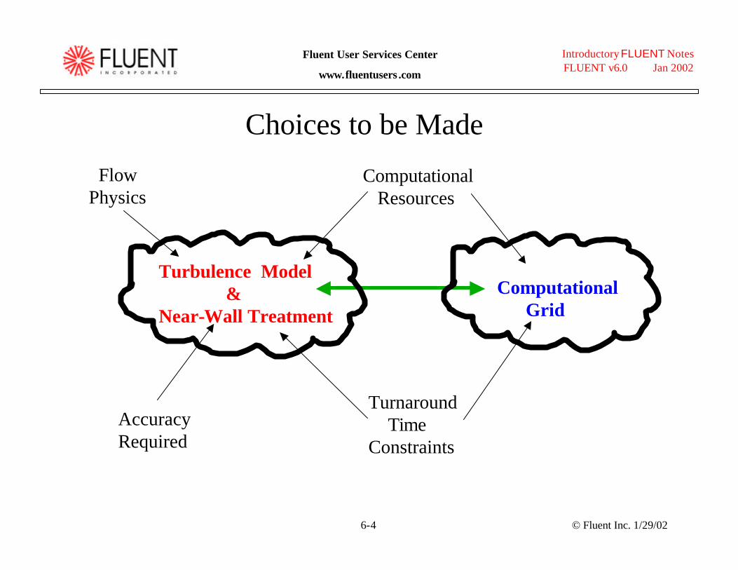
Choices to be Made

Turbulence Model&

Near-Wall Treatment

Flow Physics

AccuracyRequired

ComputationalResources

TurnaroundTime

Constraints

ComputationalGrid

© Fluent Inc. 1/29/026-5




Modeling Turbulenceu Direct numerical simulation (DNS) is the solution of the time-

dependent Navier-Stokes equations without recourse to modeling.l Mesh must be fine enough to resolve smallest eddies, yet sufficiently

large to encompass complete model.l Solution is inherently unsteady to capture convecting eddies.l DNS is only practical for simple low-Re flows.

u The need to resolve the full spectrum of scales is not necessary for most engineering applications.l Mean flow properties are generally sufficient.l Most turbulence models resolve the mean flow.

u Many different turbulence models are available and used.l There is no single, universally reliable engineering turbulence model

for wide class of flows.l Certain models contain more physics that may be better capable of

predicting more complex flows including separation, swirl, etc.

© Fluent Inc. 1/29/026-6




Modeling Approaches

u ‘Mean’ flow can be determined by solving a set of modified equations.u Two modeling approaches:

l (1) Governing equations are ensemble or time averaged (RANS-based models).n Transport equations for mean flow quantities are solved.n All scales of turbulence are modeled.n If mean flow is unsteady, ∆t is set by global unsteadiness.

l (2) Governing equations are spatially averaged (LES). n Transport equations for ‘resolvable scales.’n Resolves larger eddies; models smaller ones.n Inherently unsteady, ∆t set by small eddies.n Resulting models requires more CPU time/memory and is not practical for

the majority of engineering applications.

u Both approaches requires modeling of the scales that are averaged out.

© Fluent Inc. 1/29/026-7




RANS Modeling - Ensemble Averagingu Imagine how velocity, temperature, pressure, etc. might vary in a turbulent

flow field downstreamof a valve that has beenslightly perturbed:

u Ensemble averaging may be used to extract the mean flow properties from the instantaneous properties.

( ) ( )( )∑=

∞→=

N

n

niNi txu

NtxU

1

,1

lim,rr

U

u'i

Ui ui

t

u

( ) ( ) ( )txutxUtxu iii ,,,rrr ′+=

n identifies the ‘sample’ ID

© Fluent Inc. 1/29/026-13




Zero-Equation Models

One-Equation ModelsSpalart-Allmaras

Two-Equation ModelsStandard k-εRNG k-εRealizable k-εStandard k-ωSST k-ω

Reynolds-Stress Model

Large-Eddy Simulation

Direct Numerical Simulation

Turbulence Models in Fluent

IncreaseComputationalCostPer Iteration

Availablein FLUENT 6

RANS-basedmodels

© Fluent Inc. 1/29/026-16




Large Eddy Simulation (LES)u Motivation:

l Large eddies:n Mainly responsible for transport of momentum, energy, and other scalars,

directly affecting the mean fields.n Anisotropic, subjected to history effects, and flow-dependent, i.e., strongly

dependent on flow configuration, boundary conditions, and flow parameters.l Small eddies tend to be more isotropic, less flow-dependent, and hence more

amenable to modeling.

u Approach:l LES resolves large eddies and models only small eddies.l Equations are similar in form to RANS equations

n Dependent variables are now spatially averaged instead of time averaged.

u Large computational effortl Number of grid points, NLES ∝l Unsteady calculation

2Reτu

© Fluent Inc. 1/29/026-29




Summary: Turbulence Modeling Guidelinesu Successful turbulence modeling requires engineering judgement of:

l Flow physicsl Computer resources availablel Project requirements

n Accuracyn Turnaround time

l Turbulence models & near-wall treatments that are available

u Modeling Procedurel Calculate characteristic Re and determine if Turbulence needs modeling.l Estimate wall-adjacent cell centroid y+ first before generating mesh.l Begin with SKE (standard k-ε) and change to RNG, RKE, SKO, or SST if

needed.l Use RSM for highly swirling flows.l Use wall functions unless low-Re flow and/or complex near-wall physics are

present.

Documents

Introduction to CFD Analysis - · PDF file2-1 © Fluent Inc. 12/26/2001 Introductory FLUENT Notes FLUENT v6.0 Jan 2002 Fluent User Services Center Introduction to CFD Analysis