© Fluent Inc. 9/19/20156-1 Introductory FLUENT Notes FLUENT v6.0 Jan 2002 Fluent User Services Center Modeling Turbulent Flows

© Fluent Inc. 04/19/236-1

Introductory FLUENT Notes FLUENT v6.0 Jan 2002

Fluent User Services Center

www.fluentusers.com

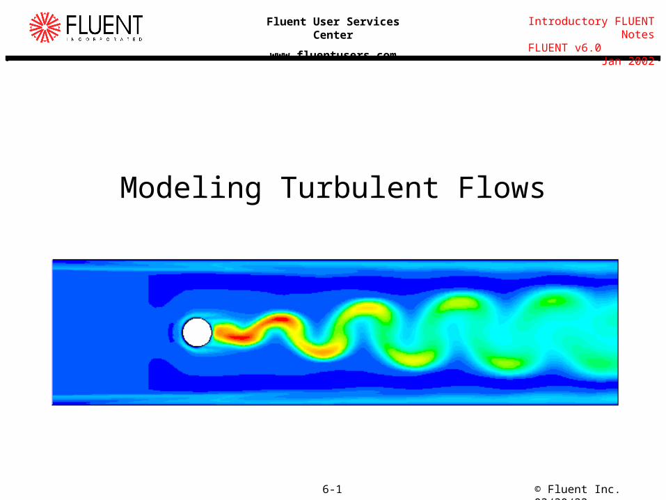
Modeling Turbulent Flows

© Fluent Inc. 04/19/236-2



www.fluentusers.com

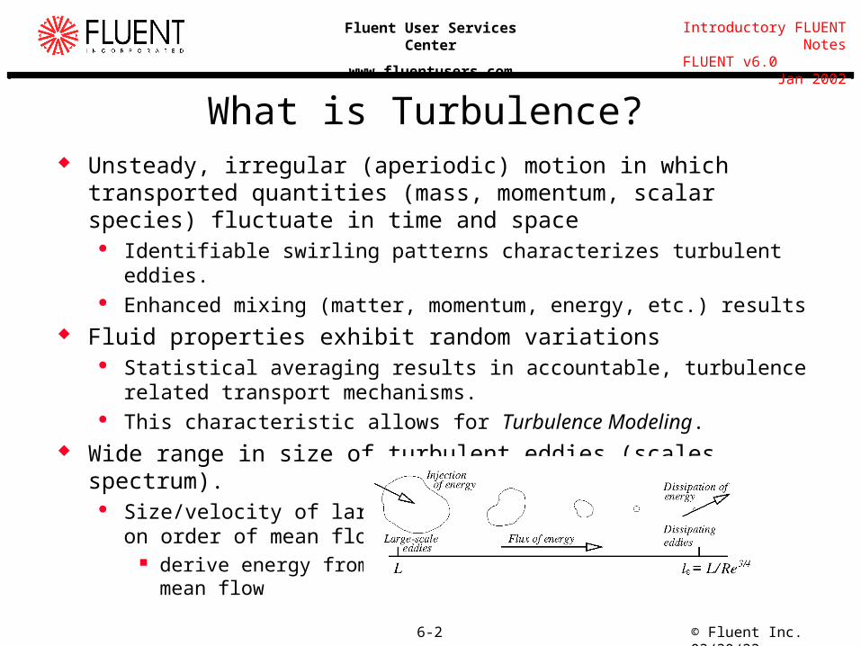
What is Turbulence? Unsteady, irregular (aperiodic) motion in which transported quantities

(mass, momentum, scalar species) fluctuate in time and space Identifiable swirling patterns characterizes turbulent eddies. Enhanced mixing (matter, momentum, energy, etc.) results

Fluid properties exhibit random variations Statistical averaging results in accountable, turbulence related transport

mechanisms. This characteristic allows for Turbulence Modeling.

Wide range in size of turbulent eddies (scales spectrum). Size/velocity of large eddies

on order of mean flow. derive energy from

mean flow

© Fluent Inc. 04/19/236-3



www.fluentusers.com

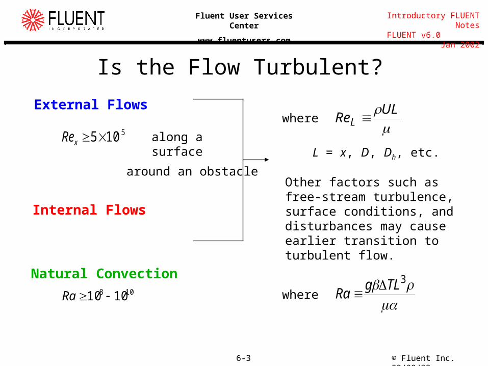
Is the Flow Turbulent?

External Flows

Internal Flows

Natural Convection

5105xRe along a surface

around an obstacle

where

UL

ReL where

Other factors such as free-stream turbulence, surface conditions, and disturbances may cause earlier transition to turbulent flow.

L = x, D, Dh, etc.

108 1010 Ra 3TLg

Ra

© Fluent Inc. 04/19/236-4



www.fluentusers.com

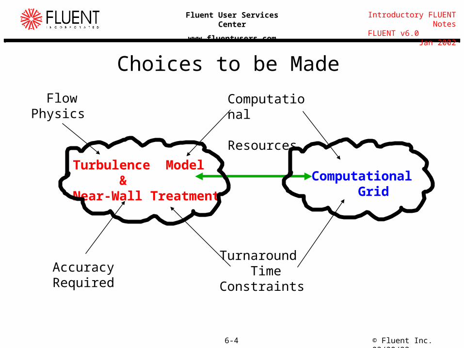
Choices to be Made

Turbulence Model&

Near-Wall Treatment

Flow Physics

AccuracyRequired

Computational Resources

Turnaround TimeConstraints

Computational Grid

© Fluent Inc. 04/19/236-5



www.fluentusers.com

Modeling Turbulence Direct numerical simulation (DNS) is the solution of the time-

dependent Navier-Stokes equations without recourse to modeling. Mesh must be fine enough to resolve smallest eddies, yet sufficiently

large to encompass complete model. Solution is inherently unsteady to capture convecting eddies. DNS is only practical for simple low-Re flows.

The need to resolve the full spectrum of scales is not necessary for most engineering applications. Mean flow properties are generally sufficient. Most turbulence models resolve the mean flow.

Many different turbulence models are available and used. There is no single, universally reliable engineering turbulence model

for wide class of flows. Certain models contain more physics that may be better capable of

predicting more complex flows including separation, swirl, etc.

© Fluent Inc. 04/19/236-6



www.fluentusers.com

Modeling Approaches

‘Mean’ flow can be determined by solving a set of modified equations. Two modeling approaches:

(1) Governing equations are ensemble or time averaged (RANS-based models). Transport equations for mean flow quantities are solved. All scales of turbulence are modeled. If mean flow is unsteady, t is set by global unsteadiness.

(2) Governing equations are spatially averaged (LES). Transport equations for ‘resolvable scales.’ Resolves larger eddies; models smaller ones. Inherently unsteady, t set by small eddies. Resulting models requires more CPU time/memory and is not practical for

the majority of engineering applications. Both approaches requires modeling of the scales that are averaged out.

© Fluent Inc. 04/19/236-7



www.fluentusers.com

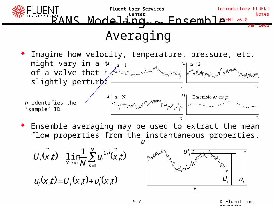
RANS Modeling - Ensemble Averaging Imagine how velocity, temperature, pressure, etc. might vary in a

turbulent flow field downstreamof a valve that has beenslightly perturbed:

Ensemble averaging may be used to extract the mean flow properties from the instantaneous properties.

N

n

ni

Ni txu

NtxU

1

,1

lim,

U

u'i

Ui ui

t

u

txutxUtxu iii ,,,

n identifies the ‘sample’ ID

© Fluent Inc. 04/19/236-8



www.fluentusers.com

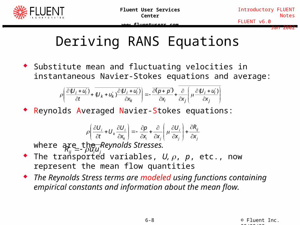
Substitute mean and fluctuating velocities in instantaneous Navier-Stokes equations and average:

Reynolds Averaged Navier-Stokes equations:

where are the Reynolds Stresses. The transported variables, U, , p, etc., now represent the mean flow

quantities The Reynolds Stress terms are modeled using functions containing

empirical constants and information about the mean flow.

j

ii

jik

iikk

ii

x

uU

xx

pp

x

uUuU

t

uU )()()(

)(

Deriving RANS Equations

j

ij

j

i

jik

ik

i

x

R

x

U

xx

p

x

UU

t

U

jiij uuR

© Fluent Inc. 04/19/236-9



www.fluentusers.com

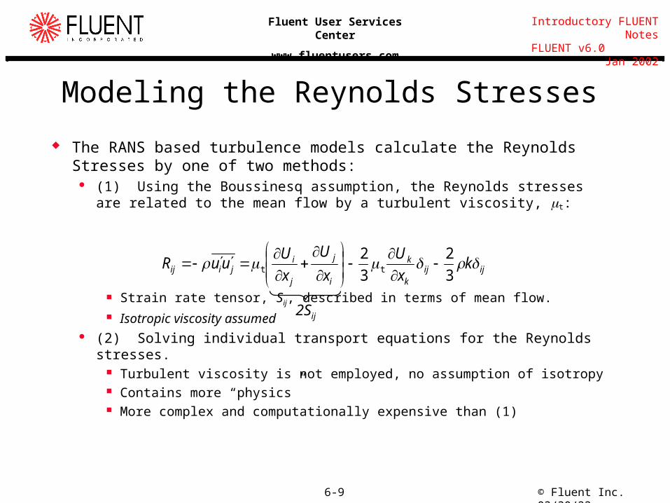
Modeling the Reynolds Stresses

The RANS based turbulence models calculate the Reynolds Stresses by one of two methods: (1) Using the Boussinesq assumption, the Reynolds stresses are related to the

mean flow by a turbulent viscosity, t:

Strain rate tensor, Sij, described in terms of mean flow. Isotropic viscosity assumed

(2) Solving individual transport equations for the Reynolds stresses. Turbulent viscosity is not employed, no assumption of isotropy Contains more “physics” More complex and computationally expensive than (1)

ijijk

k

i

j

j

ijiij k

x

U

x

U

x

UuuR

3

2

3

2tt

2Sij

© Fluent Inc. 04/19/236-10



www.fluentusers.com

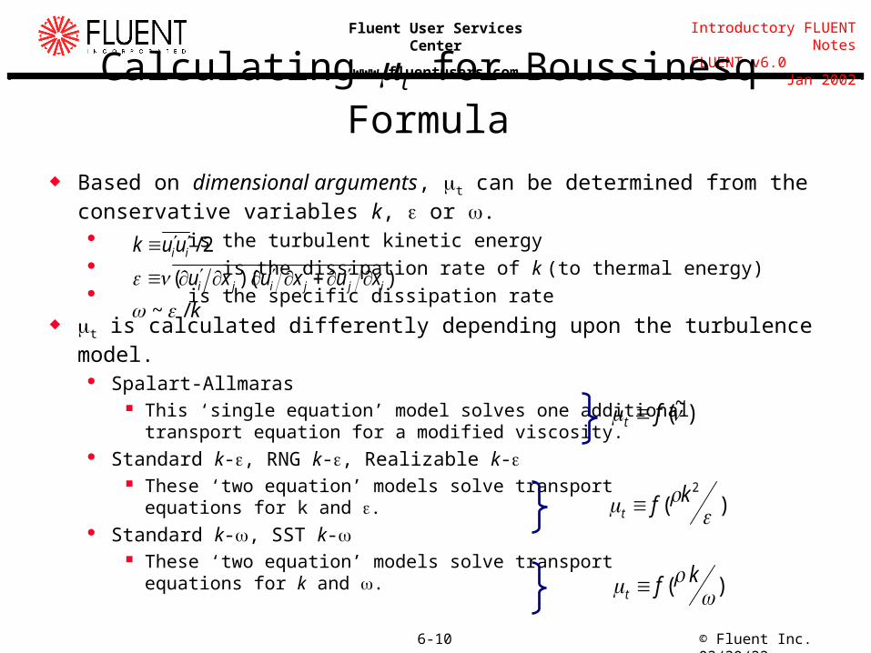
Calculating t for Boussinesq Formula

Based on dimensional arguments, t can be determined from the conservative variables k, or . is the turbulent kinetic energy is the dissipation rate of k (to thermal energy) is the specific dissipation rate

t is calculated differently depending upon the turbulence model. Spalart-Allmaras

This ‘single equation’ model solves one additional transport equation for a modified viscosity.

Standard k-, RNG k-, Realizable k- These ‘two equation’ models solve transport

equations for k and . Standard k-, SST k-

These ‘two equation’ models solve transportequations for k and .

)(2

kft

)( kft

)~( ft

2/iiuuk

))(( ijjiji xuxuxu k/~

© Fluent Inc. 04/19/236-11



www.fluentusers.com

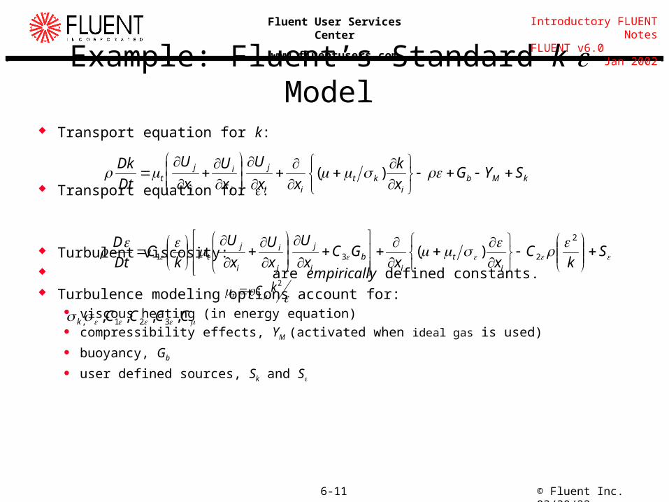
Transport equation for k:

Transport equation for :

Turbulent viscosity: are empirically defined constants. Turbulence modeling options account for:

viscous heating (in energy equation) compressibility effects, YM (activated when ideal gas is used)

buoyancy, Gb

user defined sources, Sk and S

Example: Fluent’s Standard k- Model

CCCCk ,,,, 321,

kMbi

ktii

j

j

i

i

jt SYG

x

k

xx

U

x

U

x

U

Dt

Dk

)(

Sk

Cxx

GCx

U

x

U

x

U

kC

Dt

D

it

ib

i

j

j

i

i

jt

2

231 )(

2kCt

© Fluent Inc. 04/19/236-12



www.fluentusers.com

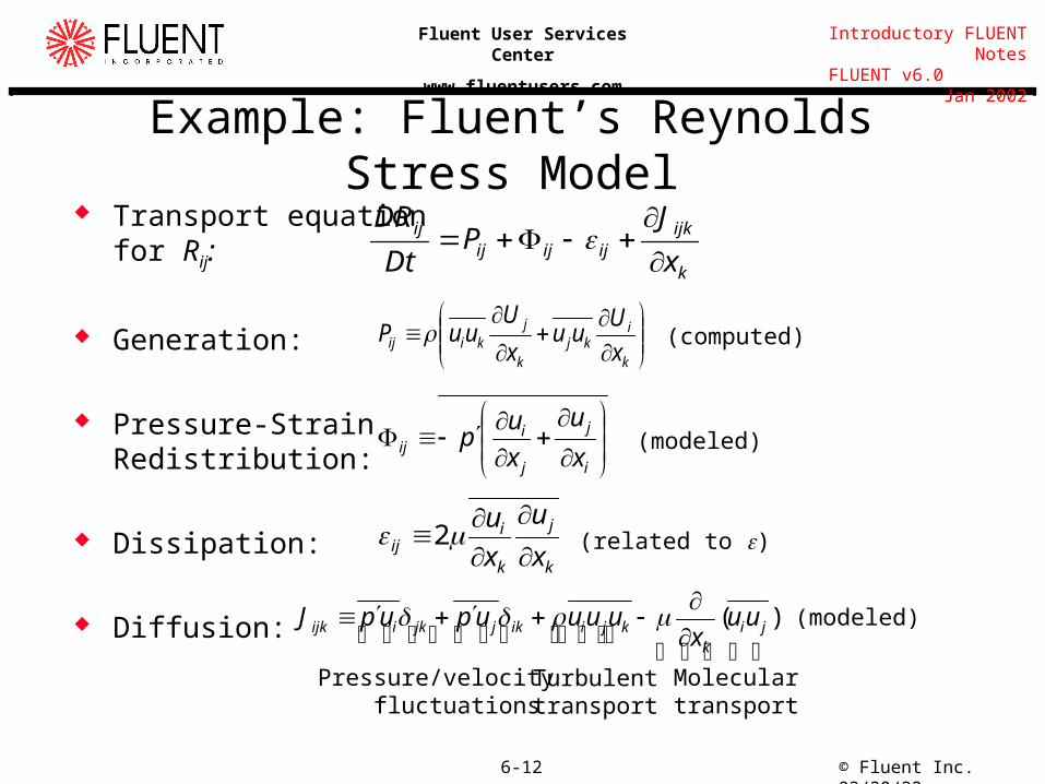
Example: Fluent’s Reynolds Stress Model

k

ijkijijij

ij

x

JP

Dt

DR

k

ikj

k

jkiij x

Uuu

x

UuuP

i

j

j

iij x

u

x

up

k

j

k

iij x

u

x

u

2

(modeled)

(related to )

(modeled)

(computed)

)( jik

kjiikjjkiijk uux

uuuupupJ

Pressure/velocity fluctuations

Turbulenttransport

Moleculartransport

Transport equation for Rij:

Generation:

Pressure-StrainRedistribution:

Dissipation:

Diffusion:

© Fluent Inc. 04/19/236-13



www.fluentusers.com

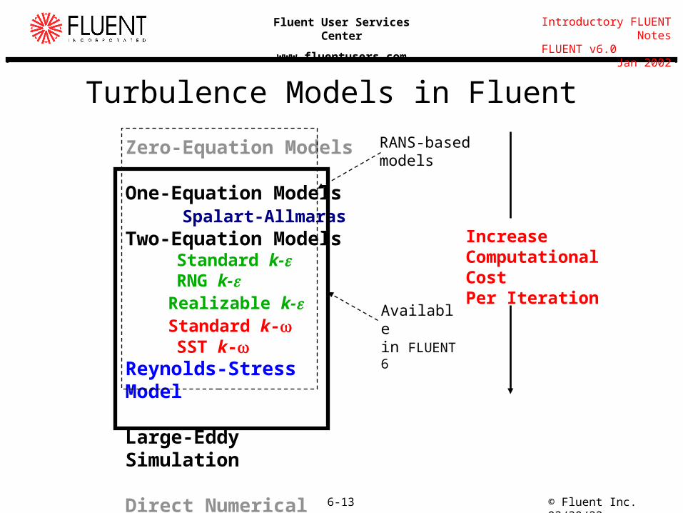
Zero-Equation Models

One-Equation Models Spalart-AllmarasTwo-Equation Models Standard k- RNG k-Realizable k-Standard k- SST k-Reynolds-Stress Model

Large-Eddy Simulation

Direct Numerical Simulation

Turbulence Models in Fluent

IncreaseComputationalCostPer Iteration

Availablein FLUENT 6

RANS-basedmodels

© Fluent Inc. 04/19/236-14



www.fluentusers.com

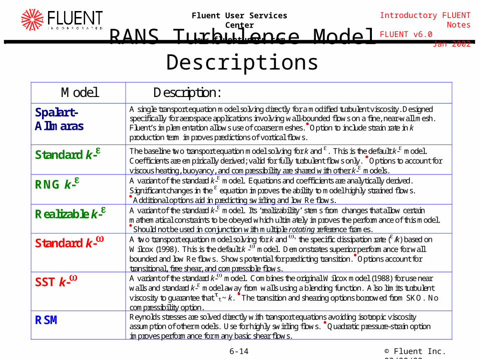
RANS Turbulence Model DescriptionsModel Description:

Spalart-Allmaras

A single transport equation model solving directly for a modified turbulent viscosity. Designedspecifically for aerospace applications involving wall-bounded flows on a fine, near-wall mesh.Fluent’s implementation allows use of coarser meshes. Option to include strain rate in kproduction term improves predictions of vortical flows.

Standard k- The baseline two transport equation model solving for k and . This is the default k-model.Coefficients are empirically derived; valid for fully turbulent flows only. Options to account forviscous heating, buoyancy, and compressibility are shared with other k- models.

RNG k- A variant of the standard k-model. Equations and coefficients are analytically derived.Significant changes in the equation improves the ability to model highly strained flows.Additional options aid in predicting swirling and low Re flows.

Realizable k- A variant of the standard k-model. Its ‘realizability’ stems from changes that allow certainmathematical constraints to be obeyed which ultimately improves the performance of this model.Should not be used in conjunction with multiple rotating reference frames.

Standard k- A two transport equation model solving for k and the specific dissipation rate (/k) based onWilcox (1998). This is the default k - model. Demonstrates superior performance for wallbounded and low Re flows. Shows potential for predicting transition. Options account fortransitional, free shear, and compressible flows.

SST k- A variant of the standard k- model. Combines the original Wilcox model (1988) for use nearwalls and standard k- model away from walls using a blending function. Also limits turbulentviscosity to guarantee that t ~ k. The transition and shearing options borrowed from SKO. Nocompressibility option.

RSM Reynolds stresses are solved directly with transport equations avoiding isotropic viscosityassumption of other models. Use for highly swirling flows. Quadratic pressure-strain optionimproves performance for many basic shear flows.

© Fluent Inc. 04/19/236-15



www.fluentusers.com

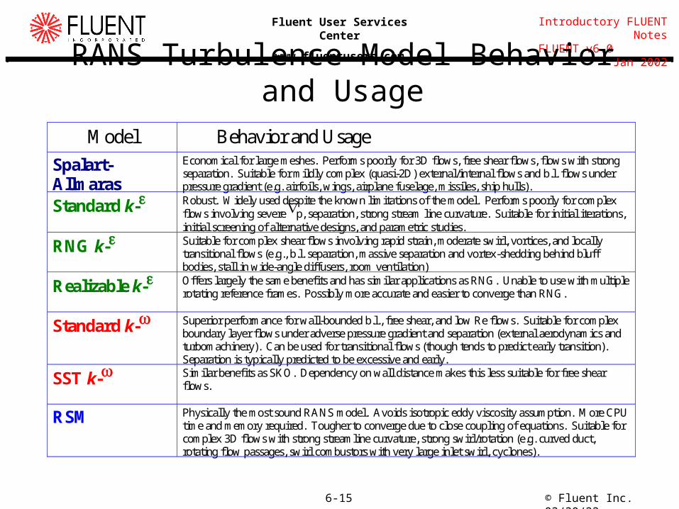
RANS Turbulence Model Behavior and UsageModel Behavior and Usage

Spalart-Allmaras

Economical for large meshes. Performs poorly for 3D flows, free shear flows, flows with strongseparation. Suitable for mildly complex (quasi-2D) external/internal flows and b.l. flows underpressure gradient (e.g. airfoils, wings, airplane fuselage, missiles, ship hulls).

Standard k- Robust. Widely used despite the known limitations of the model. Performs poorly for complexflows involving severe p, separation, strong stream line curvature. Suitable for initial iterations,initial screening of alternative designs, and parametric studies.

RNG k- Suitable for complex shear flows involving rapid strain, moderate swirl, vortices, and locallytransitional flows (e.g., b.l. separation, massive separation and vortex-shedding behind bluffbodies, stall in wide-angle diffusers, room ventilation)

Realizable k- Offers largely the same benefits and has similar applications as RNG. Unable to use with multiplerotating reference frames. Possibly more accurate and easier to converge than RNG.

Standard k- Superior performance for wall-bounded b.l., free shear, and low Re flows. Suitable for complexboundary layer flows under adverse pressure gradient and separation (external aerodynamics andturbomachinery). Can be used for transitional flows (though tends to predict early transition).Separation is typically predicted to be excessive and early.

SST k- Similar benefits as SKO. Dependency on wall distance makes this less suitable for free shearflows.

RSM Physically the most sound RANS model. Avoids isotropic eddy viscosity assumption. More CPUtime and memory required. Tougher to converge due to close coupling of equations. Suitable forcomplex 3D flows with strong streamline curvature, strong swirl/rotation (e.g. curved duct,rotating flow passages, swirl combustors with very large inlet swirl, cyclones).

© Fluent Inc. 04/19/236-16



www.fluentusers.com

Large Eddy Simulation (LES) Motivation:

Large eddies: Mainly responsible for transport of momentum, energy, and other scalars,

directly affecting the mean fields. Anisotropic, subjected to history effects, and flow-dependent, i.e., strongly

dependent on flow configuration, boundary conditions, and flow parameters. Small eddies tend to be more isotropic, less flow-dependent, and hence more

amenable to modeling. Approach:

LES resolves large eddies and models only small eddies. Equations are similar in form to RANS equations

Dependent variables are now spatially averaged instead of time averaged. Large computational effort

Number of grid points, NLES Unsteady calculation

2Reu

© Fluent Inc. 04/19/236-17



www.fluentusers.com

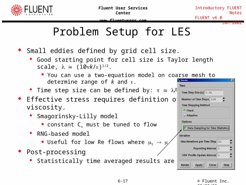
Problem Setup for LES

Small eddies defined by grid cell size. Good starting point for cell size is Taylor length scale, (10k/)1/2.

You can use a two-equation model on coarse mesh to determine range of k and .

Time step size can be defined by: U. Effective stress requires definition of Subgrid Scale

viscosity. Smagorinsky-Lilly model

constant Cs must be tuned to flow

RNG-based model Useful for low Re flows where t

Post-processing Statistically time averaged results are available.

© Fluent Inc. 04/19/236-18



www.fluentusers.com

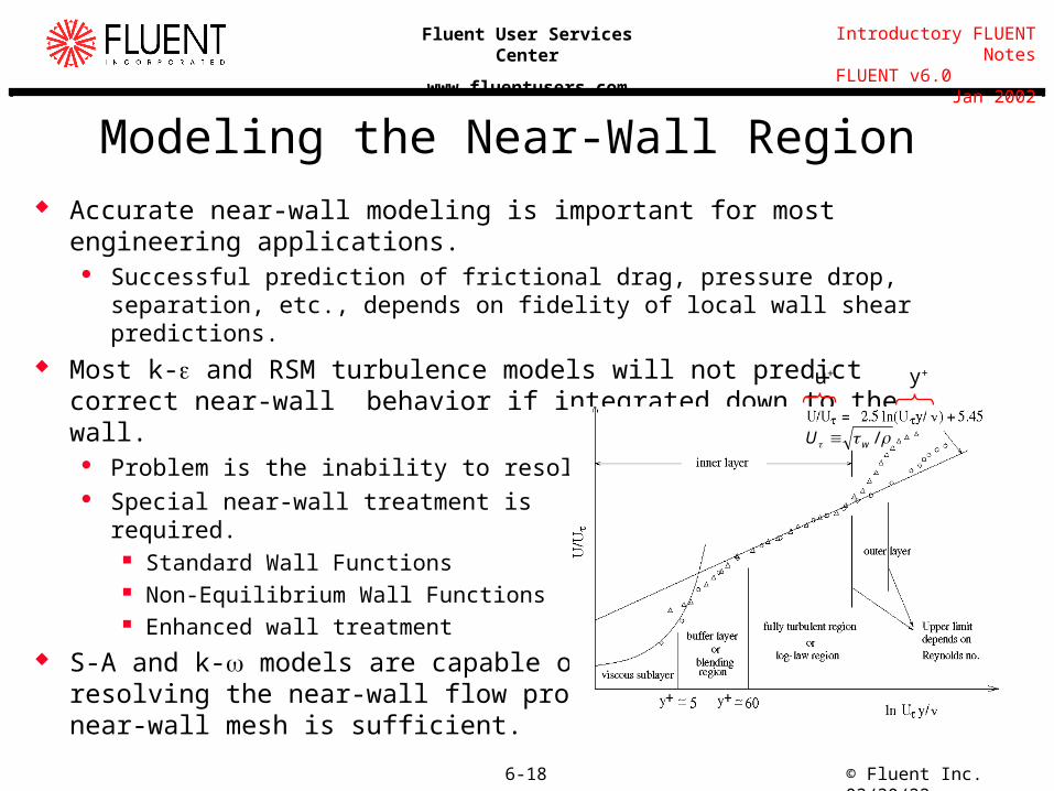
Accurate near-wall modeling is important for most engineering applications. Successful prediction of frictional drag, pressure drop, separation, etc., depends

on fidelity of local wall shear predictions. Most k- and RSM turbulence models will not predict correct near-wall

behavior if integrated down to the wall. Problem is the inability to resolve . Special near-wall treatment is

required. Standard Wall Functions Non-Equilibrium Wall Functions Enhanced wall treatment

S-A and k- models are capable ofresolving the near-wall flow provided near-wall mesh is sufficient.

u+ y+

Modeling the Near-Wall Region

/wU

© Fluent Inc. 04/19/236-19



www.fluentusers.com

In general, ‘wall functions’ are a collection or set of laws that serve as boundary conditions for momentum, energy, and species as well as for turbulence quantities.

Wall Function Options The Standard and Non-equilibrium Wall Function options

refer to specific ‘sets’ designed for high Re flows. The viscosity affected, near-wall region is not resolved. Near-wall mesh is relatively coarse. Cell center information bridged by empirically-based wall

functions.

Enhanced Wall Treatment Option This near-wall model combines the use of enhanced wall

functions and a two-layer model. Used for low-Re flows or flows with complex near-wall

phenomena. Generally requires a very fine near-wall mesh capable of

resolving the near-wall region. Turbulence models are modified for ‘inner’ layer.

Near-Wall Modeling Options

inner layer

outer layer

© Fluent Inc. 04/19/236-20



www.fluentusers.com

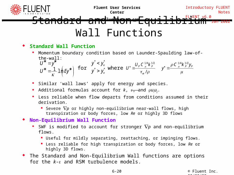
Standard Wall Function Momentum boundary condition based on Launder-Spaulding law-of-the-wall:

Similar ‘wall laws’ apply for energy and species. Additional formulas account for k, , and uiuj. Less reliable when flow departs from conditions assumed in their derivation.

Severe p or highly non-equilibrium near-wall flows, high transpiration or body forces, low Re or highly 3D flows

Non-Equilibrium Wall Function SWF is modified to account for stronger p and non-equilibrium flows.

Useful for mildly separating, reattaching, or impinging flows. Less reliable for high transpiration or body forces, low Re or highly 3D flows.

The Standard and Non-Equilibrium Wall functions are options for the k- and RSM turbulence models.

/

2/14/1

w

PP kCUU

PP ykC

y2/14/1

where

EyU ln1

yUfor

**vyy **vyy

Standard and Non-Equilibrium Wall Functions

© Fluent Inc. 04/19/236-21



www.fluentusers.com

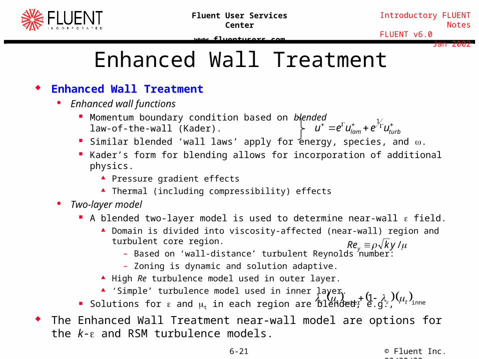
Enhanced Wall Treatment Enhanced Wall Treatment

Enhanced wall functions Momentum boundary condition based on blended

law-of-the-wall (Kader). Similar blended ‘wall laws’ apply for energy, species, and . Kader’s form for blending allows for incorporation of additional physics.

Pressure gradient effects Thermal (including compressibility) effects

Two-layer model A blended two-layer model is used to determine near-wall field.

Domain is divided into viscosity-affected (near-wall) region and turbulent core region.

– Based on ‘wall-distance’ turbulent Reynolds number:

– Zoning is dynamic and solution adaptive. High Re turbulence model used in outer layer. ‘Simple’ turbulence model used in inner layer.

Solutions for and t in each region are blended, e.g.,

The Enhanced Wall Treatment near-wall model are options for the k- and RSM turbulence models.

/ykRey

turblam ueueu1

innerouter 1 tt

© Fluent Inc. 04/19/236-22



www.fluentusers.com

Estimating Placement of First Grid Point

Ability for near-wall treatments to accurately predict near-wall flows depends on placement of wall adjacent cell centroids (cell size). For SWF and NWF, centroid should be located in

log-layer: For best results using EWT, centroid should be located in laminar

sublayer: This near-wall treatment can accommodate cells placed in the log-layer.

To determine actual size of wall adjacent cells, recall that: The skin friction coefficient can be estimated from empirical correlations:

Flat Plate- Pipe Flow-

Use post-processing to confirm near-wall mesh resolution.

2// few cUu

2.0Re0359.02 Lfc

2.0Re039.02 Dfc

30030 py

1py

uyyuyy pppp //

© Fluent Inc. 04/19/236-23



www.fluentusers.com

Near-Wall Modeling Recommended Strategy

Use SWF or NWF for most high Re applications (Re > 106) for which you cannot afford to resolve the viscous sublayer. There is little gain from resolving viscous sublayer (choice of core

turbulence model is more important). Use NWF for mildly separating, reattaching, or impinging flows.

You may consider using EWT if: The characteristic Re is low or if near wall characteristics need to be

resolved. The same or similar cases ran successfully previously with the two-

layer zonal model (in Fluent v5). The physics and near-wall mesh of the case is such that y+ is likely

to vary significantly over a wide portion of the wall region. Try to make the mesh either coarse or fine enough, and avoid

putting the wall-adjacent cells in the buffer layer (y+ = 5 ~ 30).

© Fluent Inc. 04/19/236-24



www.fluentusers.com

Setting Boundary Conditions When turbulent flow enters a domain at inlets or outlets (backflow),

boundary values for: k, and/or must be specified

Four methods for directly or indirectly specifying turbulence parameters: Explicitly input k, , or

This is the only method that allows for profile definition. Turbulence intensity and length scale

Length scale is related to size of large eddies that contain most of energy. For boundary layer flows: l 0.499

For flows downstream of grid: l opening size Turbulence intensity and hydraulic diameter

Ideally suited for duct and pipe flows Turbulence intensity and turbulent viscosity ratio

For external flows: 1 < t/ < 10

Turbulence intensity depends on upstream conditions:

jiuu

jiuu

%20/3/2 Uku/U

© Fluent Inc. 04/19/236-25



www.fluentusers.com

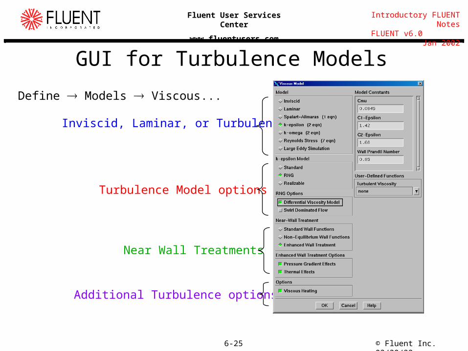
GUI for Turbulence Models

Define Models Viscous...

Turbulence Model options

Near Wall Treatments

Inviscid, Laminar, or Turbulent

Additional Turbulence options

© Fluent Inc. 04/19/236-26



www.fluentusers.com

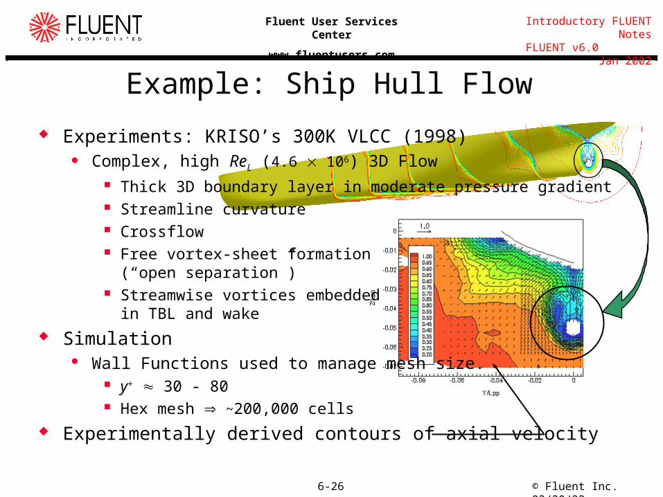
Example: Ship Hull Flow

Experiments: KRISO’s 300K VLCC (1998) Complex, high ReL (4.6 106) 3D Flow

Thick 3D boundary layer in moderate pressure gradient Streamline curvature Crossflow Free vortex-sheet formation

(“open separation”) Streamwise vortices embedded

in TBL and wake Simulation

Wall Functions used to manage mesh size. y+ 30 - 80 Hex mesh ~200,000 cells

Experimentally derived contours of axial velocity

© Fluent Inc. 04/19/236-27



www.fluentusers.com

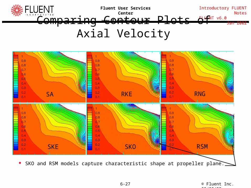
Comparing Contour Plots of Axial Velocity

SKO and RSM models capture characteristic shape at propeller plane.

SA RKE RNG

SKE SKO RSM

© Fluent Inc. 04/19/236-28



www.fluentusers.com

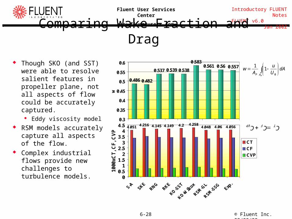
0.486 0.482

0.537 0.539 0.538

0.5830.561 0.56 0.557

0.3

0.35

0.4

0.45

0.5

0.55

0.6

w

4.051 4.216 4.145 4.149 4.2 4.2584.048 4.06 4.056

00.5

11.5

22.5

33.5

44.5

1000

xC

T,

CF

, C

VP

CT

CF

CVP

Comparing Wake Fraction and Drag

Though SKO (and SST) were able to resolve salient features in propeller plane, not all aspects of flow could be accurately captured. Eddy viscosity model

RSM models accurately capture all aspects of the flow.

Complex industrial flows provide new challenges to turbulence models.

dAU

u

Aw

PAP

0

11

VP F TC C C

© Fluent Inc. 04/19/236-29



www.fluentusers.com

Summary: Turbulence Modeling Guidelines Successful turbulence modeling requires engineering judgement of:

Flow physics Computer resources available Project requirements

Accuracy Turnaround time

Turbulence models & near-wall treatments that are available Modeling Procedure

Calculate characteristic Re and determine if Turbulence needs modeling. Estimate wall-adjacent cell centroid y+ first before generating mesh. Begin with SKE (standard k-) and change to RNG, RKE, SKO, or SST if

needed. Use RSM for highly swirling flows. Use wall functions unless low-Re flow and/or complex near-wall physics are

present.

Documents

© Fluent Inc. 9/19/20156-1 Introductory FLUENT Notes FLUENT v6.0 Jan 2002 Fluent User Services Center Modeling Turbulent Flows