CFD ANALYSIS OF UAVs USING VORSTAB, FLUENT, AND …

CFD ANALYSIS OF UAVs USING VORSTAB, FLUENT, AND ADVANCED

AIRCRAFT ANALYSIS SOFTWARE

BY

Benjamin Sweeten

Submitted to the graduate degree program in Aerospace Engineering

and the Graduate Faculty of the University of Kansas

in partial fulfillment of the requirements for the degree of

Master‟s of Science

_____________________________

Dr. Shahriar Keshmiri, Chairperson

Committee members* _____________________________*

Dr. Ray Taghavi

_____________________________*

Dr. Saeed Farokhi

_____________________________*

Dr. Richard Hale

Date Defended: April 27, 2010

ii

The Thesis Committee for Benjamin Sweeten certifies

that this is the approved Version of the following thesis:

CFD ANALYSIS OF UAVs USING VORSTAB, FLUENT, AND ADVANCED

AIRCRAFT ANALYSIS SOFTWARE

Committee:

_____________________________

Dr. Shahriar Keshmiri, Chairperson

_____________________________

Dr. Ray Taghavi

_____________________________

Dr. Saeed Farokhi

_____________________________

Dr. Richard Hale

Date approved:____________________

iii

Acknowledgements

I would like to thank NASA and the National Science Foundation for the

contributions to the University of Kansas Aerospace Engineering Department.

Without their support and funding, this research would have not taken place. Also,

thank you to Dr. Shahriar Keshmiri for his leadership and guidance during my

graduate and undergraduate career. Dr. Keshmiri helped in every aspect of my

research, from selecting classes, funding, and research topics. Thank you to Dr.

Richard Hale for his guidance on the Meridian UAV. He has high expectations of his

students, and is willing to put out the same amount of effort if not more. Thank you

to my professors that I have had throughout my education. They have given the

knowledge needed for my career path. Thank you to Dr. Lan, for allowing me to use

his program and giving me guidance during the learning process of this program.

Thank you to Andy Pritchard, the Aerospace Engineering Department‟s airplane and

power plant mechanic. Andy worked with me on many projects and research. He

offered his guidance and experience to everyone, and he was a major influence on my

graduate career. Thank you to all my fellow colleagues and students for their help.

In particular Dave Royer, Jonathan Tom, and Bill Donovan for answering and helping

with all questions that were asked of them. Without their hard work the Meridian

would have never flew. I would like to thank my family for offering their support

and anything I needed during my college career. Lastly, I would like to thank my

fiancée Jessica Donigan for her love and support. She dealt with me in a very

difficult time and has always been there for me. Thank you to everyone that I may

iv

have neglected to mention. There have been many people that gave me guidance and

support during my graduate and undergraduate career.

v

Abstract

The University of Kansas has long been involved in the research and

development of uninhabited aerial vehicles, UAVs. Currently a 1,100 lb UAV has

been designed, built, and flown from the University. A major problem with the

current design of these UAVs is that very little effort was put into the aerodynamics.

The stability and control derivatives are critical for the flight of the vehicle, and many

methods can be used to estimate them prior to flight testing. The topic of this

research is using high fidelity computer software, VORSTAB and FLUENT, to

determine the flying qualities of three different UAVs. These UAVs are the 1/3 scale

YAK-54, the MantaHawk, and the Meridian. The results found from the high fidelity

computation fluid dynamics programs were then compared to the values found from

the Advance Aircraft Analysis, AAA, software. AAA is not considered to be as

accurate as CFD, but is a very useful tool for design. Flight test data was also used to

help determine how well each program estimated the stability and control derivative

or flying qualities.

The YAK-54 results from both programs were very close to each other and

also to the flight test results. The results from the other two UAVs varied largely, due

to the complexity of the aircraft design. VORSTAB had a very difficult time

handling the complex body of the Meridian. Its results showed the aircraft was

unstable in several different modes, when this is known to not be the case after

several flight tests.

vi

From these results it was determined that VORSTAB, while a high fidelity

program, has difficulty handling aircraft with complex geometry. If the aircraft is a

traditional style aircraft with non-complex geometry VORSTAB will return highly

accurate results that are better than AAA. The benefit of AAA is that a model can be

created rather quickly and the results will typically be within an acceptable error

range. A VORSTAB model can be very time consuming to make, and this can

outweigh the improved results. It is rather simple to determine if the VORSTAB

results are valid or not, and the input file can be easily improved to increase the

accuracy of the results. It is always a smart idea to use both software programs to

check the results with one another.

FLUENT was used to determine the possible downwash issue over the

Meridian fuselage. This software is a widely accepted program that is known to

produce very accurate results. The major problem is that it is very time consuming to

make a model and requires someone with a large amount of knowledge about the

software to do so. FLUENT results showed a possibility for a large boundary layer

near the tail and flow separation at high angles of attack. These results are all

discussed throughout the report in detail.

vii

Table of Contents Page #

Acknowledgements ...................................................................................................... iii Abstract ..........................................................................................................................v

List of Figures .............................................................................................................. ix List of Tables ............................................................................................................. xiii List of Symbols ............................................................................................................xv 1 Introduction .........................................................................................................1 2 Literature Review................................................................................................3

2.1 Wavelike Characteristics of Low Reynolds Number Aerodynamics ........... 3 2.2 A Generic Stability and Control Methodology For Novel Aircraft

Conceptual Design ..................................................................................................... 4 2.3 Theoretical Aerodynamics in Today‟s Real World, Opportunities and

Challenges ................................................................................................................. 5 2.4 The Lockheed SR-71 Blackbird – A Senior Capstone Re-Engineering

Experience ................................................................................................................. 6 3 Stability and Control Derivatives........................................................................8

3.1 Longitudinal Motion ..................................................................................... 8

3.2 Lateral-Directional Motion ......................................................................... 14

3.3 Perturbed State ............................................................................................ 20 4 AAA ..................................................................................................................22 5 VORSTAB ........................................................................................................23

5.1 Creating a Model......................................................................................... 24 6 FLUENT ...........................................................................................................26

7 YAK-54.............................................................................................................29 7.1 AAA Modeling of the YAK-54 .................................................................. 32 7.2 VORSTAB Modeling of the YAK-54 ........................................................ 35

7.3 Method Comparison YAK-54..................................................................... 51 7.4 Linearized Model of the YAK-54 ............................................................... 55

8 MantaHawk .......................................................................................................56

8.1 AAA Modeling of the MantaHawk ............................................................ 57 8.2 VORSTAB Modeling of the MantaHawk .................................................. 60 8.3 Method Comparison MantaHawk ............................................................... 73 8.4 Linearized Model of the MantaHawk ......................................................... 77

9 Meridian UAV ..................................................................................................78

9.1 AAA Modeling of the Meridian ................................................................. 80 9.2 VORSTAB Modeling of the Meridian ....................................................... 83 9.3 Linearized Model of the Meridian ............................................................ 135 9.4 FLUENT Modeling of the Meridian ......................................................... 135 9.5 FLUENT Model Generation ..................................................................... 141

9.6 Method Comparison Meridian .................................................................. 158 10 Conclusions and Recommendations ...............................................................165

11 References .......................................................................................................169

viii

Table of Contents Continued

Appendix A ................................................................................................................171 Appendix B ................................................................................................................172

ix

List of Figures

Figure 1: Earth-Fixed and Body-Fixed Axes System ................................................... 9 Figure 2: YAK-54 ....................................................................................................... 29 Figure 3: Unigraphics CAD Model of YAK-54 ......................................................... 31 Figure 4: YAK-54 VORSTAB Lift Curve Slope ....................................................... 36

Figure 5: YAK-54 VORSTAB Drag Curve................................................................ 36 Figure 6: YAK-54 VORSTAB Pitching Moment Coefficient Curve ......................... 37

Figure 7: YAK-54 VORSTAB Longitudinal Derivatives .......................................... 37 Figure 8: YAK-54 VORSTAB Lateral-Directional Derivatives due to Sideslip ....... 39 Figure 9: YAK-54 VORSTAB Lateral-Directional Derivatives due to Roll Rate ..... 39 Figure 10: YAK-54 VORSTAB Lateral-Directional Derivatives due to Yaw Rate .. 40

Figure 11: YAK-54 VORSTAB Sideforce Coefficient due to Aileron Deflection .... 42 Figure 12: YAK-54 VORSTAB Rolling Moment Coefficient due to Aileron

Deflection .................................................................................................................... 42

Figure 13: YAK-54 VORSTAB Yawing Moment Coefficient due to Aileron

Deflection .................................................................................................................... 43

Figure 14: YAK-54 VORSTAB Lift Coefficient due to Elevator Deflection ............ 45

Figure 15: YAK-54 VORSTAB Drag Coefficient due to Elevator Deflection .......... 45

Figure 16: YAK-54 VORSTAB Pitching Moment Coefficient due to Elevator

Deflection .................................................................................................................... 46

Figure 17: YAK-54 VORSTAB Sideforce Coefficient due to Rudder Deflection .... 48 Figure 18: YAK-54 VORSTAB Rolling Moment Coefficient due to Rudder

Deflection .................................................................................................................... 48

Figure 19: YAK-54 VORSTAB Yawing Moment Coefficient due to Rudder

Deflection .................................................................................................................... 49

Figure 20: MantaHawk ............................................................................................... 57 Figure 21: MantaHawk VORSTAB Lift Coefficient .................................................. 61 Figure 22: MantaHawk VORSTAB Drag Coefficient................................................ 61

Figure 23: MantaHawk VORSTAB Pitching Moment Coefficient ............................ 62 Figure 24: MantaHawk VORSTAB Lift Coefficient due to Pitch Rate ..................... 62 Figure 25: MantaHawk VORSTAB Pitching Moment Coefficient due to Pitch

Rate ............................................................................................................................. 63 Figure 26: MantaHawk VORSTAB Lateral-Directional Derivatives due to

Sideslip ........................................................................................................................ 64 Figure 27: MantaHawk VORSTAB Lateral-Directional Derivatives due to Roll

Rate ............................................................................................................................. 65

Figure 28: MantaHawk VORSTAB Lateral-Directional Derivatives due to Yaw

Rate ............................................................................................................................. 65

Figure 29: MantaHawk VORSTAB Lift Coefficient due to Symmetrical Deflection 68 Figure 30: MantaHawk VORSTAB Drag Coefficient due to Symmetrical

Deflection .................................................................................................................... 68

x

List of Figures Continued

Figure 31: MantaHawk VORSTAB Pitching Moment Coefficient due to Symmetrical

Deflection .................................................................................................................... 69

Figure 32: MantaHawk VORSTAB Sideforce Coefficient due to Asymmetrical

Deflection .................................................................................................................... 71 Figure 33: MantaHawk VORSTAB Rolling Moment Coefficient due to

Asymmetrical Deflection ............................................................................................ 71 Figure 34: MantaHawk VORSTAB Yawing Moment Coefficient due to

Asymmetrical Deflection ............................................................................................ 72 Figure 35: Unigraphics CAD Model of the Meridian UAV ....................................... 79

Figure 36: Meridian Empennage Models 1 and 2 ....................................................... 86 Figure 37: Meridian VORSTAB Model 2 Lift Coefficient due to Angle of Attack... 88 Figure 38: Meridian VORSTAB Model 2 Drag Coefficient due to Angle of Attack. 88 Figure 39: Meridian VORSTAB Model 2 Pitching Moment Coefficient due to Angle

of Attack...................................................................................................................... 89 Figure 40: Meridian VORSTAB Model 2 Longitudinal Derivatives due to Pitch

Rate ............................................................................................................................. 89 Figure 41: Meridian VORSTAB Model 2 Lateral-Directional Derivatives due to

Sideslip ........................................................................................................................ 91

Figure 42: Meridian VORSTAB Model 2 Lateral-Directional Derivatives due to Roll

Rate ............................................................................................................................. 91 Figure 43: Meridian VORSTAB Model 2 Lateral-Directional Derivatives due to Yaw

Rate ............................................................................................................................. 92

Figure 44: Meridian VORSTAB Model 2 Sideforce Coefficient due to Aileron

Deflection .................................................................................................................... 95

Figure 45: Meridian VORSTAB Model 2 Rolling Moment Coefficient due to Aileron

Deflection .................................................................................................................... 95 Figure 46: Meridian VORSTAB Model 2 Yawing Moment Coefficient due to Aileron

Deflection .................................................................................................................... 96

Figure 47: Meridian VORSTAB Model 2 Lift Coefficient due to Elevator Input ..... 98 Figure 48: Meridian VORSTAB Model 2 Drag Coefficient due to Elevator Input ... 98 Figure 49: Meridian VORSTAB Model 2 Pitching Moment Coefficient due to

Elevator Input.............................................................................................................. 99 Figure 50: Meridian VORSTAB Model 2 Sideforce Coefficient due to Rudder

Input .......................................................................................................................... 101 Figure 51: Meridian VORSTAB Model 2 Rolling Moment Coefficient due to Rudder

Input .......................................................................................................................... 101 Figure 52: Meridian VORSTAB Model 2 Yawing Moment Coefficient due to Rudder

Input .......................................................................................................................... 102

Figure 53: Meridian VORSTAB Model 3 Lift Coefficient due to Angle of Attack. 103

Figure 54: Meridian VORSTAB Model 3 Drag Coefficient due to Angle of

Attack ........................................................................................................................ 104

xi


Figure 55: Meridian VORSTAB Model 3 Pitching Moment Coefficient due to Angle

of Attack.................................................................................................................... 104

Figure 56: Meridian VORSTAB Model 3 Longitudinal Coefficients due to Pitch

Rate ........................................................................................................................... 105 Figure 57: Meridian VORSTAB Model 3 Lateral-Directional Derivatives due to

Sideslip ...................................................................................................................... 106 Figure 58: Meridian VORSTAB Model 3 Lateral-Directional Derivatives due to Roll

Rate ........................................................................................................................... 106 Figure 59: Meridian VORSTAB Model 3 Lateral-Directional Derivatives due to Yaw

Rate ........................................................................................................................... 107 Figure 60: Meridian VORSTAB Model 3 Sideforce Coefficient due to Aileron

Deflection .................................................................................................................. 109 Figure 61: Meridian VORSTAB Model 3 Rolling Moment Coefficient due to Aileron

Deflection .................................................................................................................. 109 Figure 62: Meridian VORSTAB Model 3 Yawing Moment Coefficient due to Aileron

Deflection .................................................................................................................. 110 Figure 63: Meridian VORSTAB Model 3 Lift Coefficient due to Elevator Input ... 112 Figure 64: Meridian VORSTAB Model 3 Drag Coefficient at due to Elevator

Input .......................................................................................................................... 112

Figure 65: Meridian VORSTAB Model 3 Pitching Moment Coefficient due to

Elevator Input............................................................................................................ 113 Figure 66: Meridian VORSTAB Model 3 Sideforce Coefficient due to Rudder



Input .......................................................................................................................... 116

Figure 69: Meridian VORSTAB Model 4 Lift Coefficient due to Angle of Attack. 117

Figure 70: Meridian VORSTAB Model 4 Drag Coefficient due to Angle of

Attack ........................................................................................................................ 118 Figure 71: Meridian VORSTAB Model 4 Pitching Moment Coefficient due to Angle

of Attack.................................................................................................................... 118 Figure 72: Meridian VORSTAB Model 4 Longitudinal Derivatives due to Pitch

Rate ........................................................................................................................... 119 Figure 73: Meridian VORSTAB Model 4 Lateral-Directional Derivatives due to

Sideslip ...................................................................................................................... 120 Figure 74: Meridian VORSTAB Model 4 Lateral-Directional Derivatives due to Roll

Rate ........................................................................................................................... 121

Figure 75: Meridian VORSTAB Model 4 Lateral-Directional Derivatives due to

Yawing Moment ....................................................................................................... 121

Figure 76: Meridian VORSTAB Model 4 Sideforce Coefficient due to Aileron

Deflection .................................................................................................................. 124

xii



Deflection .................................................................................................................. 124

Figure 78: Meridian VORSTAB Model 4 Yawing Moment Coefficient due to Aileron

Deflection .................................................................................................................. 125 Figure 79: Meridian VORSTAB Model 4 Lift Coefficient due to Elevator Input ... 127 Figure 80: Meridian VORSTAB Model 4 Drag Coefficient due to Elevator Input . 127 Figure 81: Meridian VORSTAB Model 4 Pitching Moment Coefficient due to

Elevator Input............................................................................................................ 128 Figure 82: Meridian VORSTAB Model 4 Sideforce Coefficient due to Rudder



Input .......................................................................................................................... 131 Figure 85: Meridian Fuselage Axial Cross-Section for FLUENT ............................ 137

Figure 86: Meridian Fuselage with Farfield Divisions ............................................. 138 Figure 87: Meridian Farfield Meshes ....................................................................... 140 Figure 88: Meridian FLUENT Velocity Magnitude Profile for All Angle of

Attacks ...................................................................................................................... 145

Figure 89: Meridian FLUENT Velocity Angle Profile for All Angles of Attack .... 148 Figure 90: Velocity Profile in Boundary Layer with Favorable and Adverse Pressure

Gradient..................................................................................................................... 150

Figure 91: Velocity Profile with Flow Separation at Point S (dashed line u = 0) .... 151 Figure 92: Meridian FLUENT Total Pressure Profile for All Angles of Attack ...... 152

Figure 93: Meridian FLUENT Stream Function Profile at All Angles of Attack .... 154 Figure 94: Meridian FLUENT Vorticity Magnitude Profile at All Angles of

Attack ........................................................................................................................ 157

Figure 95: Circulation around an Airfoil Producing Lift .......................................... 158

xiii

List of Tables

Table 1: YAK-54 Lifting Surface Dimensions ........................................................... 30 Table 2: YAK-54 Flight Conditions ........................................................................... 31 Table 3: YAK-54 AAA Moment of Inertia and Trimmed Values .............................. 32 Table 4: YAK-54 AAA Longitudinal Derivatives...................................................... 33

Table 5: YAK-54 AAA Lateral-Directional Derivatives ............................................ 34 Table 6: YAK-54 AAA Stability Requirements ......................................................... 35

Table 7: YAK-54 VORSTAB Longitudinal Coefficient and Pitch Rate (1/rad) ........ 35 Table 8: YAK-54 VORSTAB Lateral-Directional Derivatives (1/rad) ...................... 38 Table 9: YAK-54 VORSTAB Lateral-Directional Due to Aileron Deflection

(1/rad) .......................................................................................................................... 41

Table 10: YAK-54 VORSTAB Longitudinal Due to Elevator Deflection (1/rad) ..... 44 Table 11: YAK-54 VORSTAB Lateral-Directional Due to Rudder Deflection

(1/rad) .......................................................................................................................... 47

Table 12: YAK-54 VORSTAB Stability Requirements ............................................. 50 Table 13: YAK-54 AAA and VORSTAB Stability and Control Comparison ........... 52

Table 14: YAK-54 Stability and Control Derivatives Typical Ranges ...................... 54

Table 15: MantaHawk AAA Longitudinal Derivatives .............................................. 58

Table 16: MantaHawk AAA Lateral-Directional Derivatives .................................... 59 Table 17: MantaHawk AAA Stability Requirements ................................................. 59

Table 18: MantaHawk VORSTAB Longitudinal Derivatives (1/rad) ........................ 60 Table 19: MantaHawk VORSTAB Lateral-Directional Derivatives (1/rad) .............. 64 Table 20: MantaHawk VORSTAB Longitudinal Derivatives due to Symmetrical

Deflection .................................................................................................................... 67 Table 21: MantaHawk VORSTAB Lateral-Directional Derivatives due to

Asymmetrical Deflections .......................................................................................... 70 Table 22: MantaHawk VORSTAB Stability Requirements ....................................... 73 Table 23: MantaHawk AAA and VORSTAB Comparison ........................................ 74

Table 24: MantaHawk Stability and Control Derivatives Typical Ranges ................. 76 Table 25: Meridian Characteristics ............................................................................. 79 Table 26: Meridian AAA Longitudinal Derivatives ................................................... 81

Table 27: Meridian AAA Lateral-Directional Derivatives ......................................... 82 Table 28: Meridian AAA Stability Requirements ...................................................... 83 Table 29: Meridian VORSTAB Model 1 Longitudinal Derivatives (1/rad) ............... 84 Table 30: Meridian VORSTAB Model 1 Lateral-Directional Derivatives (1/rad) ..... 84 Table 31: Fuselage Diameter for Meridian Models 1 and 2 ....................................... 86

Table 32: Meridian VORSTAB Model 2 Longitudinal Control Derivatives and

Affected by Pitch Rate ................................................................................................ 87

Table 33: Meridian VORSTAB Model 2 Lateral-Directional Derivatives due to

Sideslip and Roll Rate ................................................................................................. 90 Table 34: Meridian VORSTAB Model 2 Lateral-Directional Derivatives due to Yaw

Rate ............................................................................................................................. 92

xiv

List of Tables Continued

Table 35: Meridian VORSTAB Model 2 Lateral Directional Derivatives due to

Aileron Deflection ...................................................................................................... 94

Table 36: Meridian VORSTAB Model 2 Longitudinal Derivatives Affected by

Symmetrical Tail Deflections ..................................................................................... 97 Table 37: Model 2 Lateral Directional Control Derivatives Affected by Asymmetrical

Tail Deflection .......................................................................................................... 100 Table 38: Meridian VORSTAB Model 3 Longitudinal Derivatives at due to Pitch

Rate ........................................................................................................................... 103 Table 39: Meridian VORSTAB Model 3 Lateral-Directional Derivatives .............. 105

Table 40: Meridian VORSTAB Model 3 Lateral-Directional Derivative due to

Aileron Deflection .................................................................................................... 108 Table 41: Meridian VORSTAB Model 3 Longitudinal Derivatives due to

Symmetrical Tail Deflections ................................................................................... 111

Table 42: Meridian Model 3 Lateral-Directional Derivatives Affected by

Asymmetrical Tail Deflections ................................................................................. 114

Table 43: Meridian VORSTAB Model 4 Longitudinal Derivatives ........................ 117 Table 44: Meridian VORSTAB Model 4 Lateral-Directional Control Derivatives . 120 Table 45: Meridian VORSTAB Model 4 Lateral-Directional Derivatives due to

Aileron Deflection .................................................................................................... 123

Table 46: Meridian VORSTAB Model 4 Longitudinal Derivatives due to

Symmetrical Tail Deflection ..................................................................................... 126 Table 47: Meridian VORSTAB Model 4 Lateral-Directional Derivatives due to

Asymmetrical Deflection .......................................................................................... 129 Table 48: Meridian VORSTAB Stability and Control Derivatives Dr. Roskam‟s

Typical Ranges.......................................................................................................... 133 Table 49: Meridian AAA and VORSTAB Comparison ........................................... 134 Table 50: Meridian Farfield Edges ........................................................................... 139

Table 51: Meridian Edge Meshes ............................................................................. 139

Table 52: Meridian Fuselage Cross-Section FLUENT Lift and Drag ...................... 143 Table 53: Meridian Fuselage Lift and Drag Method Comparison ............................ 159 Table 54: Meridian AAA and VORSTAB Comparison ........................................... 161 Table 55: Meridian VORSTAB and AAA Stability and Control Derivatives Typical

Ranges ....................................................................................................................... 163

Table 56: YAK-54 Longitudinal Modes ................................................................... 173 Table 57: YAK-54 Lateral-Directional Modes ......................................................... 173 Table 58: MantaHawk Longitudinal Modes ............................................................. 175 Table 59: MantaHawk Lateral-Directional Modes ................................................... 176 Table 60: Meridian Model 2 Longitudinal Modes .................................................... 177

Table 61: Meridian Model 2 Lateral-Directional Modes .......................................... 178

Table 62: Meridian Model 3 Longitudinal Modes .................................................... 179

Table 63: Meridian Model 3 Lateral-Directional Modes .......................................... 180

xv

List of Symbols

Symbol Description Units

Normal

a ..................................................... Speed of Sound ..................................................... ft/sec

A or AR ........................................... Aspect Ratio ......................................................... -----

b ......................................................... Wing Span .............................................................. ft

c ............................................... Mean Geometric Chord .................................................... ft

cr ....................................................... Root Chord .............................................................. ft

ct ........................................................ Tip Chord ............................................................... ft

CD ................................................. Drag Coefficient ...................................................... -----

CD ....................... Variation of Airplane Drag with Angle of Attack .......................... 1/rad

CDe ................... Variation of Airplane Drag with Elevator Deflection ........................ 1/rad

CDu ............................... Variation of Airplane Drag with Speed .................................. 1/rad

CDq ........................... Variation of Airplane Drag with Pitch Rate ............................... 1/rad

Cl.......................................... Rolling Moment Coefficient ............................................. -----

Cl ............. Variation of Airplane Rolling Moment with Angle of Sideslip ................ 1/rad

Cla ........... Variation of Airplane Rolling Moment with Aileron Deflection ............... 1/rad

Clr ........... Variation of Airplane Rolling Moment with Rudder Deflection ............... 1/rad

Clp ..... Variation of Airplane Rolling Moment with Rate of Change of Roll Rate ....... 1/rad

Clr ..... Variation of Airplane Rolling Moment with Rate of Change of Yaw Rate ....... 1/rad

CL ................................................... Lift Coefficient ....................................................... -----

CL_ih ............ Variation of Airplane Lift with Differential Stabilizer Angle ................. 1/rad

CL ........................ Variation of Airplane Lift with Angle of Attack ........................... 1/rad

CLe .................... Variation of Airplane Lift with Elevator Deflection ......................... 1/rad

CLq ............................ Variation of Airplane Lift with Pitch Rate ................................ 1/rad

CLu ................... Variation of Airplane Lift with Dimensionless Speed ....................... 1/rad

Cm ....................................... Pitching Moment Coefficient ............................................ -----

Cm_ac .............. Pitching Moment Coefficient about Aerodynamic Center ...................... -----

Cm ............. Variation of Airplane Pitching Moment with Angle of Attack ................ 1/rad

Cme ......... Variation of Airplane Pitching Moment with Elevator Deflection .............. 1/rad

Cmq ................. Variation of Airplane Pitching Moment with Pitch Rate ..................... 1/rad

CmT ................... Variation of Airplane Pitching Moment due to Thrust ......................... -----

CmT . Variation of Airplane Pitching Moment due to Thrust with Angle of Attack .... 1/rad

Cn ......................................... Yawing Moment Coefficient ............................................ -----

Cn ............. Variation of Airplane Yawing Moment with Angle of Sideslip ................ 1/rad

Cna ........... Variation of Airplane Yawing Moment with Aileron Deflection ............... 1/rad

Cnr ........... Variation of Airplane Yawing Moment with Rudder Deflection ............... 1/rad

Cnp .... Variation of Airplane Yawing Moment with Rate of Change of Roll Rate ....... 1/rad

Cnr .... Variation of Airplane Yawing Moment with Rate of Change of Yaw Rate ....... 1/rad

CnT ....... Variation of Airplane Yawing Moment due to Thrust with Sideslip ............ 1/rad

CTx ........................... Variation of Airplane Thrust in X Direction................................. -----

CTxu ............. Variation of Airplane Thrust in X-axis with respect to speed ................... -----

Cy ............................................... Sideforce Coefficient .................................................. -----

xvi

Normal Continued

Cy ................... Variation of Airplane Sideforce with Angle of Sideslip ...................... 1/rad

Cya ................. Variation of Airplane Sideforce with Aileron Deflection..................... 1/rad

Cyr ................. Variation of Airplane Sideforce with Rudder Deflection ..................... 1/rad

Cyp .......... Variation of Airplane Sideforce with Rate of Change of Roll Rate ............. 1/rad

Cyr .......... Variation of Airplane Sideforce with Rate of Change of Yaw Rate ............. 1/rad

d/d.......................................... Downwash Gradient ................................................... -----

d/d ........................................... Sidewash Gradient .................................................... -----

D ............................................................. Drag ................................................................. lbs

e ............................................ Oswald‟s Efficiency Factor ............................................. -----

Fy ........................................................ Sideforce .............................................................. lbs

h ............................................................ Height .................................................................. ft

ih ....................................... Horizontal Tail Incidence Angle........................................... deg

Ixx, Iyy, Izz .................... Airplane Moments of Inertia about XYZ ............................ slugs-ft2

Ixz ................................ Airplane Products of Inertia about XYZ ............................. slugs-ft2

L .............................................................. Lift .................................................................. lbs

L, boundary layer ................. Flow Distance Along Body.................................................. ft

N ................................................... Yawing Moment .................................................... ft-lbs

N.D. .............................................. Non-dimensional...................................................... -----

M .................................................. Pitching Moment ................................................... ft-lbs

M∞......................................... Free Stream Mach Number .............................................. -----

p .......................................................... Roll Rate ....................................................... rad/sec

Ps ..................................................... Static Pressure ..................................................... lbs/ft2

PT .................................................... Total Pressure ..................................................... lbs/ft2

q ......................................................... Pitch Rate ...................................................... rad/sec

q =0.5V2 ............................. Aircraft Dynamic Pressure ........................................... lbs/ft

2

r........................................................... Yaw Rate ...................................................... rad/sec

u .............................................. x-component of Velocity ............................................. ft/sec

U ........................................... Axial Free Stream Velocity ........................................... ft/sec

v .............................................. y-component of Velocity ............................................. ft/sec

V .......................................................... Velocity........................................................... ft/sec

V ........................................... Volume Coefficient of Tail .............................................. -----

w ............................................. z-component of Velocity ............................................. ft/sec

S .............................................................. Area................................................................... ft2

Re ................................................ Reynolds Number ..................................................... -----

x .......................................... Axial Station Along Fuselage ................................................ ft

xac ...................Distance from Aerodynamic Center and Reference Point .......................... ft

xcg .................... Distance from Center of Gravity and Reference Point ............................. ft

xvs ................. Axial Distance Between Vertical Tail a.c and Airplane c.g. ........................ ft

2d ................................................. Two Dimensional ..................................................... -----

2ddp ............................... Two Dimensional Double Precision ....................................... -----

3d ................................................ Three Dimensional .................................................... -----

3ddp .............................. Three Dimensional Double Precision ...................................... -----

xvii

Greek

.................................................... Angle of Attack........................................................ deg

_dot .............................. Rate of Change of Angle of Attack ................................ deg/sec2

........................................................... Sideslip .............................................................. deg

..................................... Average Boundary Layer Thickness....................................... -----

* ............................................ Displacement Thickness ................................................ -----

e,a,el,r ..................................... Control Surface Deflection ............................................... deg

.........................................................Change in ........................................................... -----

............................................. Dynamic Pressure Ratio ................................................ -----

........................................................ Circulation ...................................................... m2/sec

........................................................ Taper Ratio .......................................................... -----

Kinematic Viscosity ............................................... m2/sec

.............................................................. 3.14 ................................................................ -----

........................................................... Density .......................................................... lbs/ft3

.................................... Angle of Attack Effectiveness Factor ...................................... -----

................................................ Momentum Thickness.................................................. -----

................................................... Angular Velocity ................................................ rad/sec

Stream Function ...................................................... -----

Acronyms

AAA .................................. Advanced Aircraft Analysis

CAD ..................................... Computer Aided Design

CFD ................................ Computational Fluid Dynamics

CReSIS .................... Center for Remote Sensing of Ice Sheets

KUAE ................. University of Kansas Aerospace Engineering

NSF .................................. National Science Foundation

PC ............................................. Personal Computer

TAS .............................................. True Airspeed

UAV .................................. Uninhabited Aerial Vehicle

Subscripts

a ......................................................... Aileron

B ........................................ Body Stability Axis System

e ......................................................... Elevator

el ......................................................... Elevon

f ........................................................ Fuselage

h................................................... Horizontal Tail

o....................................... Coefficient at Zero Deflection

r .......................................................... Rudder

v..................................................... Vertical Tail

w .......................................................... Wing

wf ................................................ Wing Fuselages

1............................................. Steady State Condition

1

1 Introduction

The shape and design of an aircraft can dramatically influence how the aircraft

handles and is controlled. The stability and control derivatives are essential for flight

simulation and handling qualities. There are several equations that can be used to

estimate some of the derivatives, but not all of them. These equations are just

estimations and can be magnitudes off. Therefore, better methods have to be used

before investing millions of dollars on an aircraft.

Wind tunnel tests, are a method that results in derivatives that are highly

accurate. The problems with wind tunnel tests are that it is very expensive and can be

very time consuming. Also, the wind tunnel models are scaled down to fit in the

tunnel, and this can have a dramatic change on the results, since the results do not

always scale up as easily. Air will flow over a smaller body differently than a larger

body, due to the changes in Reynolds number and other flow characteristics. Using

an experienced wind tunnel expert and a highly accurate tunnel can minimize these

problems, but will be very expensive. Over the past couple of decades computer

simulation has become much more prevalent. Computational Fluid Dynamic

software is much more accurate than it once was and is becoming more user friendly,

but it still requires an expert to create a 3-D full aircraft CFD model. The mesh

generation for a model can be difficult and requires a great deal of experience. This

software is expensive to purchase, but can be used over and over again. Also, many

different test cases can be run to determine flying qualities in various situations.

There are also several different programs that are readily available that can produce

2

high fidelity results, and some of these programs can be purchased at a reasonable

price.

Three different computer programs were used to determine the stability and

control derivatives on three different UAVs. Two of the aircrafts were being

designed and built to fly while the other one was already a production aircraft. The

1/3 scaled YAK-54 model was a production aircraft purchased by the University of

Kansas, and the Meridian and MantaHawk were designed at the University of Kansas.

The Meridian is a 1,100 lb aircraft that was designed to fly in the Polar Regions.

Advanced Aircraft Analysis (AAA) and VORSTAB were used on all three aircraft

and FLUENT was also used on the Meridian. FLUENT is a very high fidelity CFD

program, but requires a large amount of experience and time. High level CFD

programs can be very expensive and time consuming when performing aerodynamic

analysis. This is why engineers prefer to use engineering level programs, such as

AAA, to generate the derivatives quickly. The main goal of this research was to use

high fidelity CFD programs to test the validity of these engineering level programs.

The stability and control derivatives found from each software program were

compared to each other and conclusions about the software were drawn.

3

2 Literature Review

It is a wise idea to examine current and past research going on in the field of

study. This gives the researcher a chance to see what is currently going on, or has

previously been examined in the past. It can also give the researcher ideas on topics

and experiments to conduct. The research that was conducted in this paper is

aerodynamic analysis, using high fidelity CFD programs, to determine the stability

and control derivatives of UAVs with low Reynolds numbers. Therefore, the

literature review topics consisted of stability and control analysis software, low

Reynolds number aerodynamics, and the CFD software that was used in this research.

A brief summary of each article will be given and then the conclusion drawn from

these papers.

2.1 Wavelike Characteristics of Low Reynolds Number Aerodynamics

Lifting surfaces will demonstrate several uncharacteristic flow patterns when

flown at a low Reynolds number. These patterns include a drag increase greater than

the rate of increasing lift, acoustic disturbances, and variances in drag across the span

of the lifting surface. This has a great effect on the design of micro or small UAVs

since they have rather small Reynolds numbers. Spanwise flow can usually be

ignored at higher velocities, but due to the low Reynolds number the flow can travel

in the spanwise direction. Using velocity potential theory, boundary layer theory, and

sinusoidal wave theory, the drag variation can be modeled as a sinusoidal wave along

the span. These results were then comparedt to the research conducted by Guglielmo

4

and Selig, where the drag magnitude was observed to be happening in a wave form

along the span. The goal of this research was not to exactly match the Guglielmo and

Selig data, but to demonstrate that the drag magnitude and flow can be modeled using

sinusoidal wave theory. This goal was successfully accomplished even though it did

not match the trend observed by Guglielmo and Selig. All of this can be found in

detail in Ref [1].

This research shows how the low Reynolds number can affect the flow around

the aircraft‟s lifting surfaces. At low speeds the drag magnitude can vary along the

span of the lifting surface, and in turn this can dramatically affect the other stability

and control of the aircraft. If the flow is traveling at different speeds and in different

directions (spanwise) the aircraft will not react how it typically would at higher

speeds. The control surfaces would not have the same impact when the flow is

varying.

2.2 A Generic Stability and Control Methodology For Novel Aircraft

Conceptual Design

Stability and control is the most serious requirement for flight safety, and yet

there is not a standard or reliable method for determining stability and control in the

design phase. There are several methods used and many are considered acceptable

within the industry. A major weakness, of most methods, is the design and sizing of

the control effectors. Currently very simple methods are used for the sizing, and are

done so in the cruise, landing, and take-off conditions of the flight envelope. This

5

research shows that sizing should be done so in the grey areas of the flight envelope,

where non-linear aerodynamics prevail.

A method for generating stability and control was designed over a four year

period and is called AeroMesh. This method is capable of handling both

conventional and unconventional and symmetric or asymmetric flight vehicles.

Design constraints and various flight conditions are first implemented into the

program. An input file is then created for a CFD program called VORSTAB. This

CFD software will estimate the stability and control derivatives as well as determine

the size, position, and hinge lines of the control effectors. A 6 degree-of-freedom

model is then used to determine stability and control in the trimmed and untrimmed

condition. This 6-DOF model uses control power to determines the stability and

control derivatives in the trimmed and untrimmed conditions. All information was

taken from Ref [2].

This research shows just how important a high fidelity CFD program can be

do the design of the control effectors and their sizing. The design criteria are at the

extremes of the flight envelope, so the control effectors are designed at the point of

non-linear aerodynamics. Using VORSTAB can help eliminate the use of simple

methods that are low fidelity.

2.3 Theoretical Aerodynamics in Today’s Real World, Opportunities and

Challenges

CFD has revolutionized the aerodynamic industry, but it still faces many

challenges in predicting and controlling various flows. These flows include UAV

6

low Reynolds number, high angle of attack, boundary layer transition, three-

dimensional separation, and others. Since this is the case it is wise to combine

theoretical, computational, and experimental approaches when analyzing the flow.

These problems that a typical CFD program, has with the flow, is discussed and ways

to analytically solve these problems are given. Multiple approaches are applied to the

flow to find solutions. Using all three of the solution methods allows the users to see

the short comings of each method. It is a very important and critical skill set to know

and understand how to set up a problem up from the beginning, and then make

approximations using mathematical and physics-based models. This principle should

then be applied to a modern computational method. All information was taken from

Ref [3].

It can be seen that not only a CFD program should be used during the design

process, but also other methods. The research in this report covers both analytical

methods, AAA, and high fidelity methods, VORSTAB and FLUENT. Understanding

how to set up problems is very important due to the high complexity of modern CFD

programs. A small error in the input can dramatically influence the results. It is also

very important for the user to be able to interpret the results, and this skill set comes

from understanding the theoretical methods.

2.4 The Lockheed SR-71 Blackbird – A Senior Capstone Re-Engineering

Experience

At the University of Texas at Arlington, the senior aerospace class re-

engineered the Lockheed SR-71 Blackbird in a two part design course. Currently in

7

the aerospace industry, it is very rare for a company to start a design from scratch, but

rather add to or modify previous research.

There were no changes made to the SR-71 model, but rather the aircraft was

reanalyzed. A CAD model of the aircraft was created, and from there the stability

and control derivatives were determined in a two different ways. VORSTAB was the

primary method for obtaining the derivatives, but also the Dr. Roskam method was

used. The Roskam method is outlined in an eight book series about aircraft design.

This second method is the same as using the AAA software. Both methods

derivatives were then compared to the actual SR-71 data. The VORSTAB results

were off by an order of magnitude, but followed the correct trends with the exception

of the yawing moment coefficient due to sideslip and yawing moment coefficient due

to roll rate. All other aspects of the design process were completed ranging from

aircraft systems to flight performance. All information was taken from Ref [4].

The re-engineering of the SR-71 by the senior design class at the University of

Texas at Arlington is very similar to the topic of this thesis. Several methods of

analysis were used to determine the stability and control derivatives, and the results

were then compared to one another.

8

3 Stability and Control Derivatives

The stability and control derivatives come from the aerodynamic forces and

moments acting on upon the aircraft components. These components are defined as

the wings, tails, fuselage, and any other surface on the aircraft. The flow around an

entire aircraft is too complex to allow formulas to determine the derivatives. Wind

tunnel tests or high fidelity computational fluid dynamics should be used to estimate

the control derivatives with a high level of accuracy. To define and understand the

stability and control derivatives one must have a basic understanding of aerodynamic

principles; it will be assumed that the reader has this basic knowledge. The aircraft

forces and moments are broken into two distinct directional motions, longitudinal

motion and lateral-directional motion. Coupling between longitudinal and lateral-

directional dynamics is assumed to be zero for stability and control derivative

estimation.

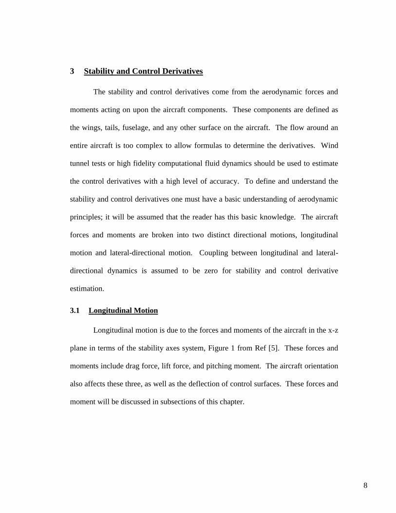
3.1 Longitudinal Motion

Longitudinal motion is due to the forces and moments of the aircraft in the x-z

plane in terms of the stability axes system, Figure 1 from Ref [5]. These forces and

moments include drag force, lift force, and pitching moment. The aircraft orientation

also affects these three, as well as the deflection of control surfaces. These forces and

moment will be discussed in subsections of this chapter.

9

Figure 1: Earth-Fixed and Body-Fixed Axes System (From Ref [5])

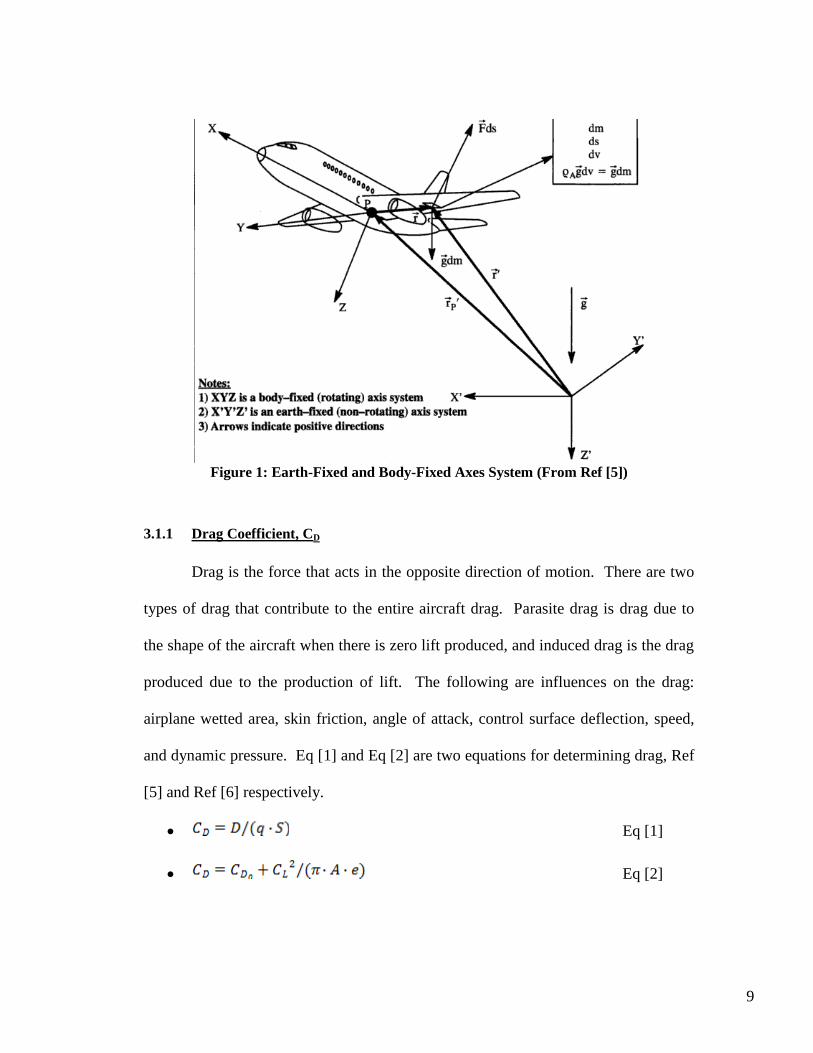
3.1.1 Drag Coefficient, CD

Drag is the force that acts in the opposite direction of motion. There are two

types of drag that contribute to the entire aircraft drag. Parasite drag is drag due to

the shape of the aircraft when there is zero lift produced, and induced drag is the drag

produced due to the production of lift. The following are influences on the drag:

airplane wetted area, skin friction, angle of attack, control surface deflection, speed,

and dynamic pressure. Eq [1] and Eq [2] are two equations for determining drag, Ref

[5] and Ref [6] respectively.

Eq [1]

Eq [2]

10

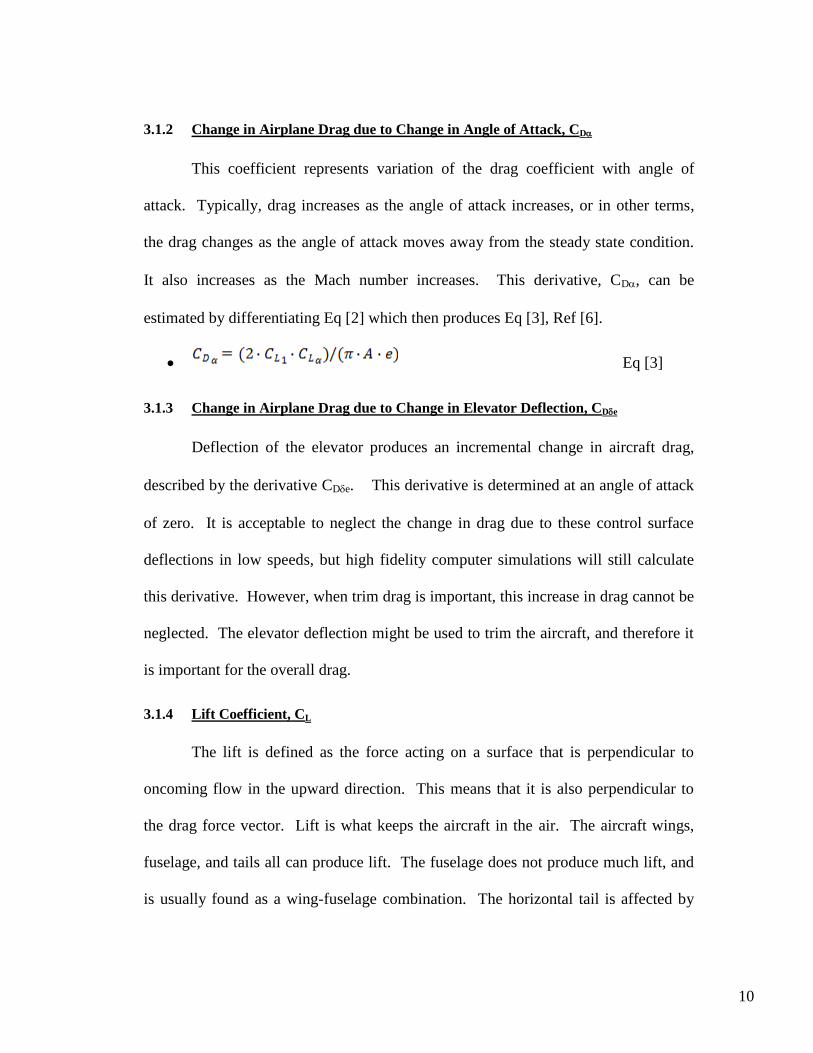
3.1.2 Change in Airplane Drag due to Change in Angle of Attack, CD

This coefficient represents variation of the drag coefficient with angle of

attack. Typically, drag increases as the angle of attack increases, or in other terms,

the drag changes as the angle of attack moves away from the steady state condition.

It also increases as the Mach number increases. This derivative, CD, can be

estimated by differentiating Eq [2] which then produces Eq [3], Ref [6].

Eq [3]

3.1.3 Change in Airplane Drag due to Change in Elevator Deflection, CDe

Deflection of the elevator produces an incremental change in aircraft drag,

described by the derivative CDe. This derivative is determined at an angle of attack

of zero. It is acceptable to neglect the change in drag due to these control surface

deflections in low speeds, but high fidelity computer simulations will still calculate

this derivative. However, when trim drag is important, this increase in drag cannot be

neglected. The elevator deflection might be used to trim the aircraft, and therefore it

is important for the overall drag.

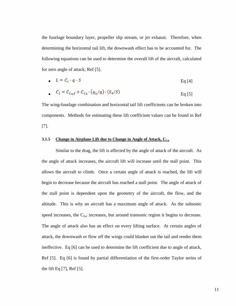
3.1.4 Lift Coefficient, CL

The lift is defined as the force acting on a surface that is perpendicular to

oncoming flow in the upward direction. This means that it is also perpendicular to

the drag force vector. Lift is what keeps the aircraft in the air. The aircraft wings,

fuselage, and tails all can produce lift. The fuselage does not produce much lift, and

is usually found as a wing-fuselage combination. The horizontal tail is affected by

11

the fuselage boundary layer, propeller slip stream, or jet exhaust. Therefore, when

determining the horizontal tail lift, the downwash effect has to be accounted for. The

following equations can be used to determine the overall lift of the aircraft, calculated

for zero angle of attack, Ref [5].

Eq [4]

Eq [5]

The wing-fuselage combination and horizontal tail lift coefficients can be broken into

components. Methods for estimating these lift coefficient values can be found in Ref

[7].

3.1.5 Change in Airplane Lift due to Change in Angle of Attack, CL

Similar to the drag, the lift is affected by the angle of attack of the aircraft. As

the angle of attack increases, the aircraft lift will increase until the stall point. This

allows the aircraft to climb. Once a certain angle of attack is reached, the lift will

begin to decrease because the aircraft has reached a stall point. The angle of attack of

the stall point is dependent upon the geometry of the aircraft, the flow, and the

altitude. This is why an aircraft has a maximum angle of attack. As the subsonic

speed increases, the CL increases, but around transonic region it begins to decrease.

The angle of attack also has an effect on every lifting surface. At certain angles of

attack, the downwash or flow off the wings could blanket out the tail and render them

ineffective. Eq [6] can be used to determine the lift coefficient due to angle of attack,

Ref [5]. Eq [6] is found by partial differentiation of the first-order Taylor series of

the lift Eq [7], Ref [5].

12

Eq [6]

Eq [7]

3.1.6 Change in Airplane Lift due to Change in Elevator Deflection, CLe

The deflection of the elevator will change the camber of the horizontal tail

airfoils and therefore change the lift of those airfoils. Highly cambered airfoils

usually have higher lift. Therefore, depending on the camber direction of the

horizontal tail and the direction of deflection, the lift of the horizontal tail will

increase or decrease. The effect of the elevator deflection on the total aircraft lift

coefficient can be found in Eq [8], Ref [5]. This is also found by partial

differentiation of the first-order Taylor series of lift Eq [7], Ref [5].

Eq [8]

3.1.7 Pitching Moment Coefficient, Cm

This is defined as the aerodynamic force that creates a moment that causes the

aircraft to pitch, or rotate upwards and downwards. Lifting forces create this resultant

force that causes the aircraft to pitch. The point that the aircraft rotates about is

typically defined as the center of gravity. Center of pressure is defined as the point at

which the pitching moment coefficient is equal to zero. Aerodynamic center is the

point about which the pitching moment coefficient does not vary with angle of attack.

As the angle of attack changes the center of pressure location will change. These two

points create the pitching moment coefficient; the center of pressure location changes

cause the change in the pitching moment. Most aircraft are inherently stable as long

13

as the center of gravity is ahead of the aerodynamic center. Elevator deflection and

angle of attack can dramatically change the pitching moment. The following

equations define the pitching moment coefficient and estimation of this value, Ref

[5].

Eq [9]

Eq [10]

3.1.8 Change in Airplane Pitching Moment due to Change in Angle of Attack, Cm

As stated previously, the center of pressure can move forward and aft as the

angle of attack changes. This results in a changing moment arm and an increasing or

decreasing pitching moment. The angle of attack also changes the lift on the aircraft,

and therefore changes the aerodynamic force that creates the pitching moment. This

derivative, Cm is called the static longitudinal stability derivative which should be

negative for an inherently longitudinally stable aircraft. For example, if the aircraft

that is statically stable is pitched upward it naturally returns to steady state and

pitches down or vice-versa if pitched downward. If it was not stable, the aircraft

would want to continue pitching upward and could flip over. The horizontal tail has a

large affect on this since it is used to pitch the aircraft. Horizontal tail incidence

angle can dramatically affect this derivative due to the lift it creates on the tail. Eq

[11] can be used to estimate this derivative, Ref [5].

14

Eq [11]

3.1.9 Change in Pitching Moment due to Change in Elevator Deflection, Cme

This derivative is referred to as the longitudinal control power derivative and

is typically negative. The effectiveness of the elevator is basically due to the volume

coefficient of the horizontal tail, Eq [12], and the angle of attack effectiveness of the

elevator, , Ref [5]. The larger the size of the elevator is, the more effect it has on the

pitching moment. For example, a fully moving horizontal tail has just as much effect

as the incidence of the horizontal tail. Eq [13] is used to estimate the derivative, Ref

[5].

Eq [12]

Eq [13]

3.2 Lateral-Directional Motion

The rolling motion is referred to as the lateral motion, and the yawing motion

is referred to as the directional motion. These two motions are results of control

surface deflections and sideforces, where sideslip plays a large role in lateral-

directional motion. This is the angle of directional rotation from the aircraft

centerline to the direction of the wind. The sideslip angle can be thought of as the

directional angle of attack. The forces and moments that are defined in the lateral-

15

directional motion are sideforce, yawing moment, and rolling moment. Similar to

longitudinal control, there are several variables that affect these forces and moments.

3.2.1 Rolling Moment, Cl

The rolling moment is the aircraft‟s rotation about the x-axis in the stability

coordinate system. Several different things can cause and influence the rolling

moment, and those are sideslip, angle of attack, the moment reference center (usually

center of gravity), deflection of control surfaces, and airspeed. The control surfaces

that affect the rolling moment are the aileron (lateral control surface) and rudder

(directional control surface). Elevator deflection influence can usually be ignored

since the deflections are symmetrical and theoretically cancel each other out. Eq [14]

is the dimensional form of the rolling moment and Eq [15] shows the first order

Taylor series form of the rolling moment, Ref [5].

Eq [14]

Eq [15]

3.2.2 Change in Airplane Rolling Moment due to Change in Sideslip, Cl

This derivative is often referred to as the airplane dihedral effect. The reason

for this is because the airplane dihedral angle can have a huge influence on the rolling

moment especially when at a sideslip. If the aircraft is at a sideslip and has a dihedral

angle on the wings, one of the wings will be hit with more air than the other. This

will cause a higher lift on that wing and in turn cause the airplane to roll. Rolling

moment derivative due to sideslip can be estimated by summing the dihedral effect of

16

the individual components of the aircraft, Eq [16], Ref [5]. There are many factors

that play into the individual components‟ dihedral effect. For example, the wings‟

location on the fuselage can affect the direction that the aircraft will want to roll. The

vertical tail will also see a higher sideforce when the aircraft is at a sideslip. For a

detailed explanation and ways to estimate the individual components of the dihedral

effect refer to Ref [5].

Eq [16]

3.2.3 Change in Airplane Rolling Moment due to Change in Aileron Deflection, Cla

A positive aileron deflection is defined as the right aileron up and the left

aileron down. This produces a rolling moment by decreasing the lift on the right

wing due to the negative camber of the aileron, and increasing the lift on the left wing

due to the positive camber of the aileron. These aileron deflections will also produce

a yawing moment, and this is why most ailerons are deflected differentially. This

differential deflection will help minimize the yawing moment that is produced. Flow

separation can also occur with large aileron deflections, and this can reduce the

effectiveness of the ailerons.

3.2.4 Change in Airplane Rolling Moment due to Change in Rudder Deflection, Clr

The purpose of the rudder is to produce a yawing moment, but due to the

typical location of the vertical tail and rudder a rolling moment is produced. With the

rudder deflected, the free stream air will encounter the rudder and produce a

sideforce. The resultant sideforce is typically located above the center of gravity and

17

will produce this rolling moment. This derivative is usually positive, but at high

angles of attack it can switch signs because of the vertical tail moment arm location

changes. Eq [17] shows how to estimate this derivative, Ref [5].

Eq [17]

3.2.5 Sideforce Coefficient, Cy

This is the aerodynamic force that causes the aircraft to yaw and can cause a

rolling moment if above or below the center of gravity. With zero angle of attack,

sideslip, and control surface deflection, the sideforce should equal zero for a

symmetrical aircraft. The sideforce is a result of sideslip, angle of attack, control

surface deflection, and symmetry of aircraft. For an unsymmetrical aircraft, a

sideforce could be produced from the side that has a larger amount of surface area

being hit by the free stream air. Eq [18] calculates the dimensional sideforce and Eq

[19] shows the first order Taylor series, Ref [5].

Eq [18]

Eq [19]

3.2.6 Change in Airplane Sideforce due to Change in Sideslip, Cy

Similar to the effect sideslip has on rolling moment, this derivative can be

broken down into individual components. The wings‟ contribution depends on the

dihedral angle. A larger dihedral will produce a large sideforce, because there is

more surface area for the sideslip free stream to contact; however, the wings‟

contribution is generally negligible. Fuselage contribution depends on its shape and

18

size. Large fuselages have more contact surface area to produce larger sideforces.

The vertical tail can produce a large sideforce due to the large moment arm from the

center of gravity and the size of the tail. This derivative can be estimated using

methods found in Ref [7].

3.2.7 Change in Airplane Sideforce due to Change in Aileron Deflection, Cya

This contribution to the sideforce is very small and more often than not

negligible. If these rolling moment controls are close to a vertical surface the

sideforce cannot be neglected. This happens by the increase in lift on one side and a

decrease on the opposite side. These changes in lift are actually changes in pressure

which, if close to a vertical surface, can produce a sideforce. Wind tunnel tests have

to be completed to measure this in a reliable fashion.

3.2.8 Change in Airplane Sideforce due to Change in Rudder Deflection, Cyr

The rudder has a large influence on the sideforce. The purpose of a rudder

deflection is to create a sideforce that will produce a yawing moment. Depending on

the location it will also produce a small rolling moment. This sideforce depends on

the size of the vertical tail in relation to the wings. The lift curve slope of the vertical

tail also plays into the influence of sideforce. The sideforce contribution of the

rudder can be determined using Eq [20], Ref [5].

Eq [20]

19

3.2.9 Yawing Moment, Cn

The aircraft yawing moment is the rotation about the z-axis in the stability

coordinate system. For a symmetrical aircraft the yawing moment is equal to zero for

zero angle of attack, sideslip, and control surface deflections. The same things that

influence the rolling moment influence the yawing moment. Those influences are

angle of attack, sideslip, speed, control surface deflections, and location of the

moment reference center. Eq [21] is the dimensional form of the yawing moment and

Eq [22] is the first order Taylor series, Ref [5].

Eq [21]

Eq [22]

3.2.10 Change in Yawing Moment due to Change in Sideslip, Cn

This derivative is referred to as the static directional stability and plays a large

role in Dutch roll and spiral dynamics. The derivative can be estimated by summing

the components of the aircraft, Eq [23], Ref [5]. The wings‟ influence can be

neglected since the flow is usually in line with the airfoil. The fuselage, on the other

hand, can play a large role, but it depends on the shape and the amount of projected

side area forward or aft of the center of gravity. Another impact on the fuselage

contribution is the Munk effect, which shifts the aerodynamic center forward. The

vertical tail also has a significant contribution. The size and location of the vertical

tail determines the amount of contribution it has. Eq [24] shows the contribution of

the vertical tail, Ref [5].

20

Eq [23]

Eq [24]

3.2.11 Change in Yawing Moment due to Change in Aileron Deflection, Cna

With aileron deflections, the lift increases on the aileron with positive camber,

downward deflection, and the lift decreases on the aileron with negative camber,

upward deflection. An increase in lift will cause an increase in induced drag, and a

decrease in lift will cause a decrease in induced drag. Higher drag on one wing will

cause the aircraft to yaw. This type of yawing moment, called an adverse yawing

moment, is undesirable because it tends to yaw the aircraft out of an intended turn.

Therefore, either pilot input or differential ailerons are used to prevent the aircraft

from yawing.

3.2.12 Change in Yawing Moment due to Change in Rudder Deflection, Cnr

This derivative depends largely on the size of the vertical tail in relation to the

wings. The lift curve slope of the vertical tail also plays a large role. The location of

the vertical tail will determine the moment arm. Also, the size of the rudder will

influence the yawing moment. Eq [25] is used to estimate the derivative, Ref [5].

Eq [25]

3.3 Perturbed State

A perturbed state flight condition is defined as one for which all motion

variables are defined relative to a known steady state flight condition, Ref [5]. It can

21

be thought of as the aircraft‟s motion varying from the steady state condition. These

variations are increases or decreases in velocity in any direction, or acceleration in

any direction or motion.

The longitudinal motion is influenced by a change in velocity in the u and w

direction if the velocity is broken down into three components, u, v, and w. Pitch

rate, q, also affects the longitudinal derivatives. It is assumed that the pitch rate has a

negligible influence on the lateral-directional motion.

Some of the lateral-directional perturbation influences are the v component of

a velocity change, yaw rate, and roll rate. Small roll rate perturbations cause non-

symmetrical changes in local angles of attack over the lifting surface. It can easily be

visualized how these changes in angle of attack will influence the lateral-directional

derivatives. Small yaw rate perturbations cause changes in the local velocity on the

lifting surfaces. They also cause changes in the angle of attack of the vertical tail.

There are also perturbation influences from changes in the flight angles. For

example, these flight angles can be the sideslip angle or angle of attack.

22

4 AAA

Advanced Aircraft Analysis, AAA, is a software program developed by

DARcorporation that is an aircraft stability, control, and design tool. It is widely

accepted as the industry standard and is used in 45 countries. The program follows

the Dr. Roskam method of preliminary aircraft design. Although the program will

model any size aircraft, the lower limit of the Reynolds number for calculations is

3e6. This means modeling of smaller aircraft may be inaccurate to some degree.

The software works for preliminary design all the way up to Class II cost

analysis. Geometric and flight characteristics of the aircraft being modeled are input,

and with a simple click of „calculate‟, outputs are produced. This program helps

eliminate errors in calculations and spreadsheets. If the designer does not understand

how something is being determined, there is a help button that shows all of the

equations used for each variable. This helps eliminate the black box feeling that

comes from most modeling software programs. If this help is not enough, the books

the program is based on are Airplane Design I-VIII, Airplane Flight Dynamics and

Automatic Flight Controls, Parts I and II, by Dr. Jan Roskam, and Airplane

Aerodynamics and Performance, by Dr. C.T. Lan and Dr. Jan Roskam, Ref [8].

AAA is used before the aircraft is ever built, but can also be used to model

production vehicles. Using AAA, the stability and control derivatives can be found

and compared with actual flight test data. Doing this helps validate the software,

allowing the designer to be more comfortable with the results AAA produces when

designing an aircraft from scratch.

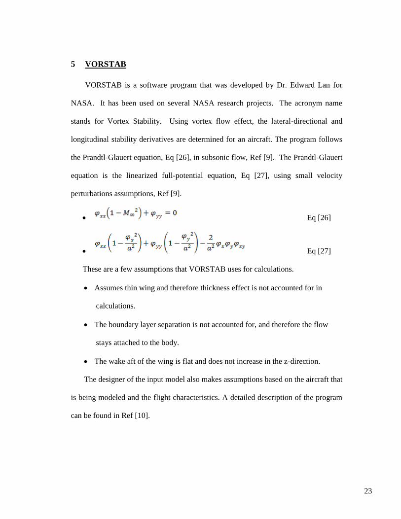
23

5 VORSTAB

VORSTAB is a software program that was developed by Dr. Edward Lan for

NASA. It has been used on several NASA research projects. The acronym name

stands for Vortex Stability. Using vortex flow effect, the lateral-directional and

longitudinal stability derivatives are determined for an aircraft. The program follows

the Prandtl-Glauert equation, Eq [26], in subsonic flow, Ref [9]. The Prandtl-Glauert

equation is the linearized full-potential equation, Eq [27], using small velocity

perturbations assumptions, Ref [9].

Eq [26]

Eq [27]

These are a few assumptions that VORSTAB uses for calculations.

Assumes thin wing and therefore thickness effect is not accounted for in

calculations.

The boundary layer separation is not accounted for, and therefore the flow

stays attached to the body.

The wake aft of the wing is flat and does not increase in the z-direction.

The designer of the input model also makes assumptions based on the aircraft that

is being modeled and the flight characteristics. A detailed description of the program

can be found in Ref [10].

24

5.1 Creating a Model

VORSTAB runs an input file that the designer creates. There are 83 groups

that are used to describe the aircraft and the test cases that are to be run. These

groups break down a step by step procedure for creating the model and allow the

designer to trouble shoot more easily. Not every group is used to describe the aircraft

that is being modeled, and many groups are repeated several times. Detailed

descriptions of the groups are found in Ref [11].

To create a model of the aircraft the designer needs to have detailed

schematics of the geometry. Typically, this geometry comes from a CAD model.

Using the CAD model the designer can find all of the geometry needed for

VORSTAB. The software does not require that a fuselage be present in the model.

The first step in creating the model is to specify the number of lifting surfaces that are

to be modeled. These lifting surfaces include wings, horizontal tail, vertical tail, v-

tail, and canards. The level flight geometry of each lifting surface is input into

VORSTAB. If this is not done, the program assumes that the geometry is at zero

angle of attack, when it might actually be more or less. For example, when the

Meridian sits on the ground, the wings and tail are at a higher angle of attack when

compared to level flight. The input lifting surface geometry required includes airfoil

characteristics (thickness and camber), location in terms of distance from reference

point (example: nose of aircraft), dihedral, twist, location of control surfaces, and

much more. Also needed is the lift coefficient, drag coefficient, and pitching moment

coefficient with respect to angle of attack. This step is repeated for each lifting

25

surface. Next, the fuselage data is input into VORSTAB. The geometry needed for

this includes cross-section shape, camber, axial locations from a reference point, and

much more. The more cross-sections used in this model, the more accurate the results

will be. It must be made sure that the lifting surfaces are not inside of the fuselage.

The fuselage model is also created in level flight for the same reason as the lifting

surfaces. Scaling the input file is very important. The entire aircraft is scaled to a

size where the largest cross-sectional radius of the fuselage is no larger than a

measurement of 1 in any unit system.

Next, the type of case that is to be run is described. This includes the flight

condition, control surface deflection angles, angle of attack, and more. With the input

file complete, VORSTAB can run. If there is an error in the input file, the output file

will stop at the group with the problem. This is a great advantage to find simple

problems in the input file that the designer overlooked. VORSTAB also creates a file

that can be opened with TECplot to see a graphical representation of the model. This

graphical representation allows the designer to visually determine if something looks

wrong with the model created.

26

6 FLUENT

FLUENT is a commercially sold computational fluid dynamics program that

is widely accepted for its high fidelity. The program has many different capabilities

and functions. Both 2-demensional and 3-demensional cases can be tested with

laminar, invisid, or turbulent flow. Depending on the model and flow type, the

designer chooses which flow field type is best. For large models, over 200,000 cells

and a coupled solver, a standard PC with single memory cannot process the model.

Super computers with multiple processors must be used to solve these larger models.

The following are the steps followed to run a FLUENT model.

Step 1: Create a GAMBIT model with a mesh for the flow field. GAMBIT is a

software program that allows the designer to easily create a geometric model of the

object being tested. The geometry of the object and the flow field around the model

are created. The size of the mesh will dramatically affect the accuracy of the results

and the processing time.

Step 2: Export the mesh so that it can be imported into FLUENT.

Step 3: With FLUENT opened, select either 2-D or 3-D, depending on the mesh

created in GAMBIT. There is also 2ddp and 3ddp. The “dp” stands for double

precision, and is more accurate than just the standard 2d or 3d. Case run time is

larger for this method, but the accuracy of the results is important to the validity of

the model.

27

Step 4: Import the mesh and run a check to see if there are errors in the mesh.

The size of the mesh can also be seen to verify that there are not too many cells to run

the test on a standard PC.

Step 5: Choose the type of solver: segregated or coupled. Coupled solver

requires much more computer memory. The „solver‟ is the method that the program

uses to solve the equations.

Segregated solver- solves the equations one by one. Momentum, continuity,

energy (if compressible flow), turbulent factor, and then check for

convergence.

Coupled solver- solves the same equations as the segregated solver, but does

this simultaneously instead of one by one.

Step 6: Choose the type of flow: laminar, invisid, or turbulent. If choosing

turbulent flow select the turbulent model to use. It is difficult to determine the most

accurate turbulent model without testing several different ones. The accuracy

depends on the mesh shape and flow pattern. Research has shown that the most

accurate method for aerodynamics is Spalart-Allmaras.

Step 7: Set the fluid properties and boundary conditions. The fluid properties

include but are not limited to density, viscosity, velocity, wall friction, and much

more.

Step 8: Select the solution controls and discretization methods. This depends on

the shape of the body and type of flow. A description of each solution and

28

discretization method should be read before the designer chooses which one is best

for their model. The FLUENT online help menu should be used for these questions.

SIMPLE and SIMPLEC are good choices for non-complicated flow problems

(such as laminar flow).

PISO is used for transient flows.

Step 9: Set the residuals and turn on what parameters are to be monitored. For

example, the lift and drag of the body can be monitored.

Step 10: Iterate until the solution converges. The convergence criteria is

determined by setting the residuals.

These steps can slightly vary from mesh to mesh, but in general these ten

steps allow the user to run a FLUENT model.

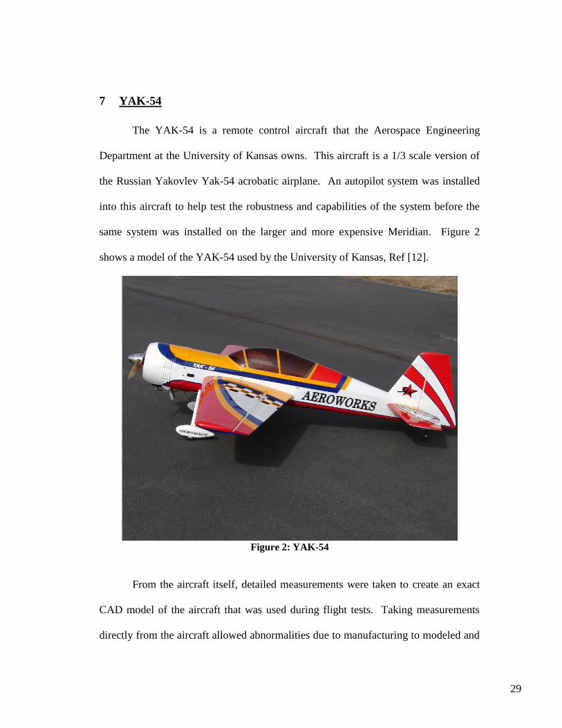
29

7 YAK-54

The YAK-54 is a remote control aircraft that the Aerospace Engineering

Department at the University of Kansas owns. This aircraft is a 1/3 scale version of

the Russian Yakovlev Yak-54 acrobatic airplane. An autopilot system was installed

into this aircraft to help test the robustness and capabilities of the system before the

same system was installed on the larger and more expensive Meridian. Figure 2

shows a model of the YAK-54 used by the University of Kansas, Ref [12].

Figure 2: YAK-54

From the aircraft itself, detailed measurements were taken to create an exact

CAD model of the aircraft that was used during flight tests. Taking measurements

directly from the aircraft allowed abnormalities due to manufacturing to modeled and

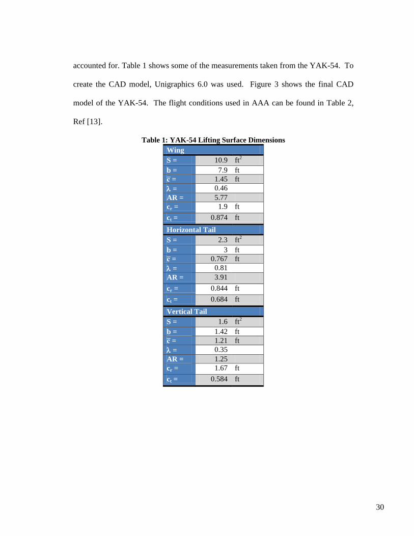
30

accounted for. Table 1 shows some of the measurements taken from the YAK-54. To

create the CAD model, Unigraphics 6.0 was used. Figure 3 shows the final CAD

model of the YAK-54. The flight conditions used in AAA can be found in Table 2,

Ref [13].

Table 1: YAK-54 Lifting Surface Dimensions

Wing

S = 10.9 ft2

b = 7.9 ft

c = 1.45 ft

= 0.46

AR = 5.77

cr = 1.9 ft

ct = 0.874 ft

Horizontal Tail

S = 2.3 ft2

b = 3 ft

c = 0.767 ft

= 0.81

AR = 3.91

cr = 0.844 ft

ct = 0.684 ft

Vertical Tail

S = 1.6 ft2

b = 1.42 ft

c = 1.21 ft

= 0.35

AR = 1.25

cr = 1.67 ft

ct = 0.584 ft

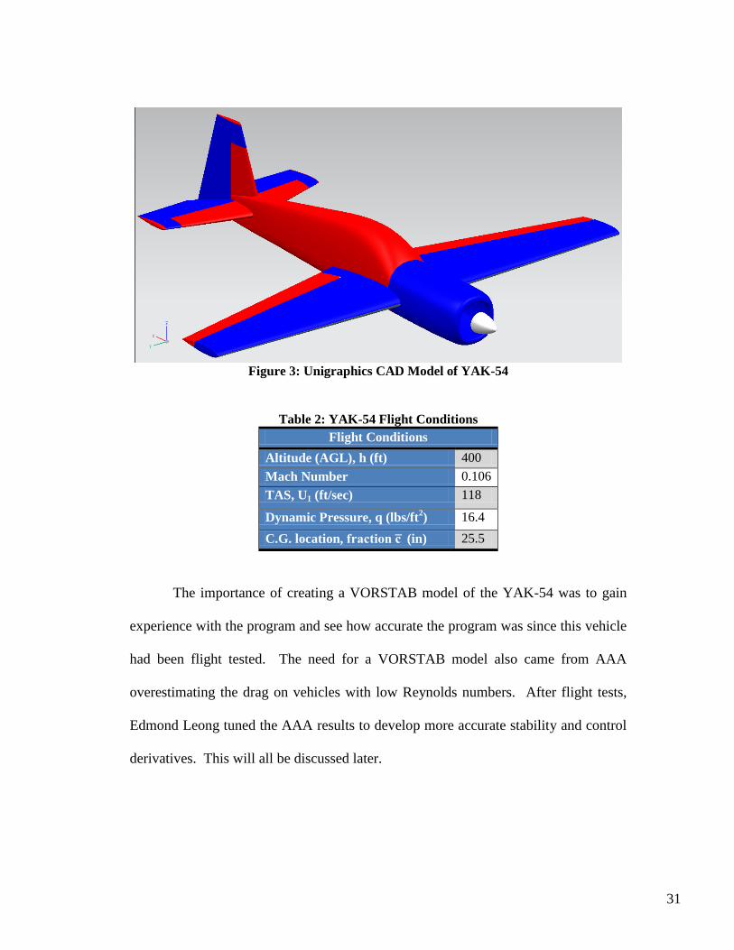
31

Figure 3: Unigraphics CAD Model of YAK-54

Table 2: YAK-54 Flight Conditions

Flight Conditions

Altitude (AGL), h (ft) 400

Mach Number 0.106

TAS, U1 (ft/sec) 118

Dynamic Pressure, q (lbs/ft2) 16.4

C.G. location, fraction c (in) 25.5

The importance of creating a VORSTAB model of the YAK-54 was to gain

experience with the program and see how accurate the program was since this vehicle

had been flight tested. The need for a VORSTAB model also came from AAA

overestimating the drag on vehicles with low Reynolds numbers. After flight tests,

Edmond Leong tuned the AAA results to develop more accurate stability and control

derivatives. This will all be discussed later.

32

7.1 AAA Modeling of the YAK-54

AAA was used to determine the YAK-54‟s dimensionless longitudinal and

lateral-directional stability and control derivatives. Table 3 shows the trimmed

condition values of the aircraft, Table 4 shows the longitudinal derivatives, and Table

5 shows the lateral-directional derivatives, all results were taken from Ref [13].

Table 6 shows the stability requirements for the YAK-54 produced by AAA, Ref

[13].

Table 3: YAK-54 AAA Moment of Inertia and Trimmed Values

Mass Data

Weight (lbs) 28

IxxB (slug-ft2) 1.09

IyyB (slug-ft2) 2.11

IzzB (slug-ft2) 3.04

IxzB (slug-ft2) 0.05

Steady State-Trimmed

CL1 0.147

CD1 0.053

CTx1 0.052

Cm1 -0.002

CmT1 0.0009

Angle of attack, 1 (deg) 1.79

Elevator Deflection Angle, e1 (deg) -0.69

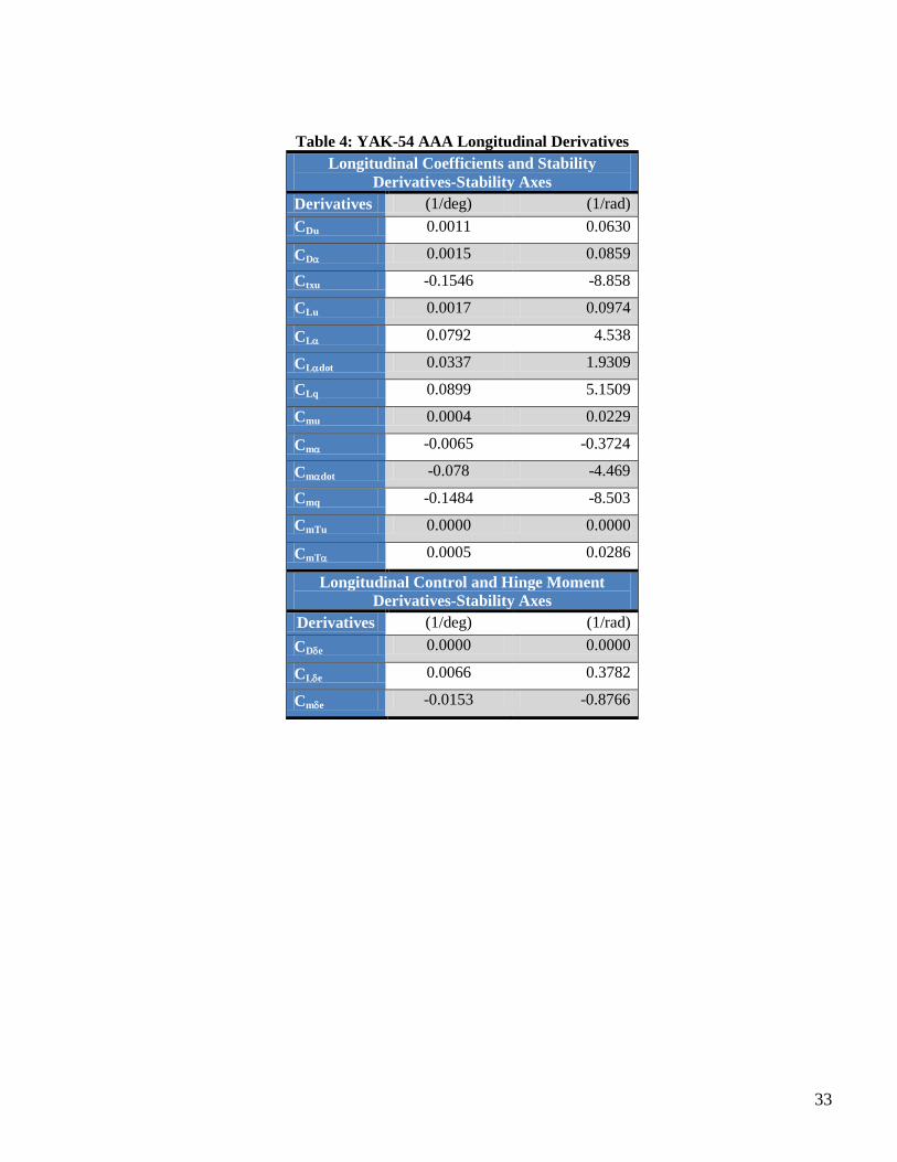
33

Table 4: YAK-54 AAA Longitudinal Derivatives

Longitudinal Coefficients and Stability

Derivatives-Stability Axes

Derivatives (1/deg) (1/rad)

CDu 0.0011 0.0630

CD 0.0015 0.0859

Ctxu -0.1546 -8.858

CLu 0.0017 0.0974

CL 0.0792 4.538

CLdot 0.0337 1.9309

CLq 0.0899 5.1509

Cmu 0.0004 0.0229

Cm -0.0065 -0.3724

Cmdot -0.078 -4.469

Cmq -0.1484 -8.503

CmTu 0.0000 0.0000

CmT 0.0005 0.0286

Longitudinal Control and Hinge Moment



CDe 0.0000 0.0000

CLe 0.0066 0.3782

Cme -0.0153 -0.8766

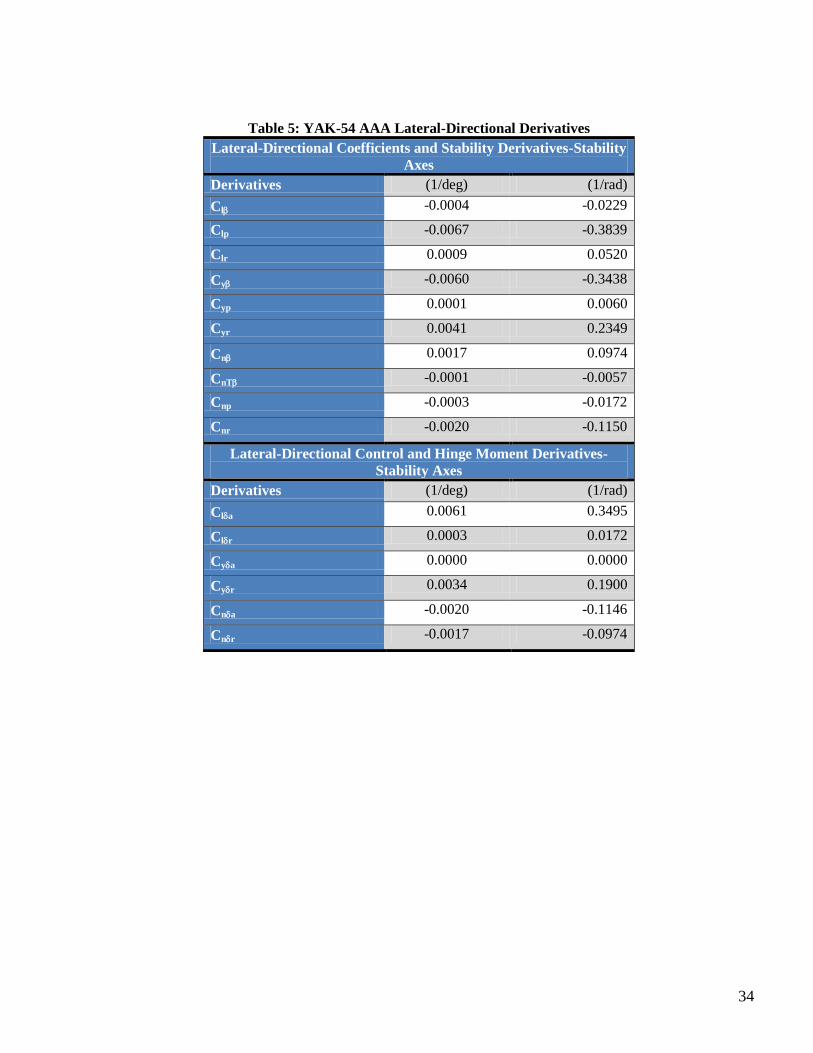
34

Table 5: YAK-54 AAA Lateral-Directional Derivatives

Lateral-Directional Coefficients and Stability Derivatives-Stability

Axes


Cl -0.0004 -0.0229

Clp -0.0067 -0.3839

Clr 0.0009 0.0520

Cy -0.0060 -0.3438

Cyp 0.0001 0.0060

Cyr 0.0041 0.2349

Cn 0.0017 0.0974

CnT -0.0001 -0.0057

Cnp -0.0003 -0.0172

Cnr -0.0020 -0.1150

Lateral-Directional Control and Hinge Moment Derivatives-

Stability Axes


Cla 0.0061 0.3495

Clr 0.0003 0.0172

Cya 0.0000 0.0000

Cyr 0.0034 0.1900

Cna -0.0020 -0.1146

Cnr -0.0017 -0.0974

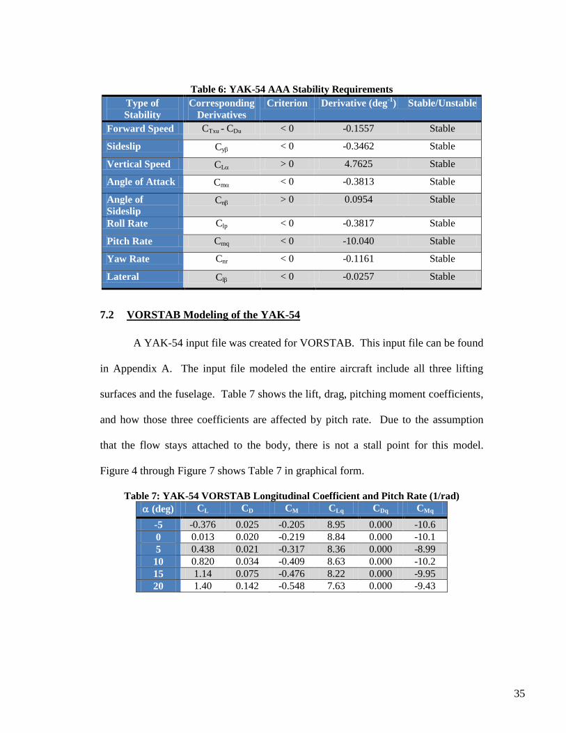
35

Table 6: YAK-54 AAA Stability Requirements

Type of

Stability

Corresponding

Derivatives

Criterion Derivative (deg-1

) Stable/Unstable

Forward Speed CTxu - CDu < 0 -0.1557 Stable

Sideslip Cy < 0 -0.3462 Stable

Vertical Speed CL > 0 4.7625 Stable

Angle of Attack Cm < 0 -0.3813 Stable

Angle of

Sideslip Cn > 0 0.0954 Stable

Roll Rate Clp < 0 -0.3817 Stable

Pitch Rate Cmq < 0 -10.040 Stable

Yaw Rate Cnr < 0 -0.1161 Stable

Lateral Cl < 0 -0.0257 Stable

7.2 VORSTAB Modeling of the YAK-54

A YAK-54 input file was created for VORSTAB. This input file can be found

in Appendix A. The input file modeled the entire aircraft include all three lifting

surfaces and the fuselage. Table 7 shows the lift, drag, pitching moment coefficients,

and how those three coefficients are affected by pitch rate. Due to the assumption

that the flow stays attached to the body, there is not a stall point for this model.

Figure 4 through Figure 7 shows Table 7 in graphical form.

Table 7: YAK-54 VORSTAB Longitudinal Coefficient and Pitch Rate (1/rad)

(deg) CL CD CM CLq CDq CMq

-5 -0.376 0.025 -0.205 8.95 0.000 -10.6

0 0.013 0.020 -0.219 8.84 0.000 -10.1

5 0.438 0.021 -0.317 8.36 0.000 -8.99

10 0.820 0.034 -0.409 8.63 0.000 -10.2

15 1.14 0.075 -0.476 8.22 0.000 -9.95

20 1.40 0.142 -0.548 7.63 0.000 -9.43

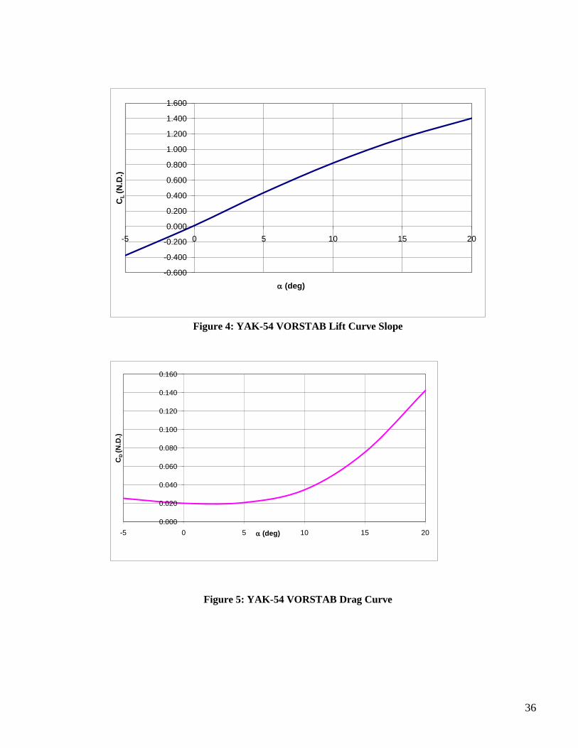
36

-0.600

-0.400

-0.200

0.000

0.200

0.400

0.600

0.800

1.000

1.200

1.400

1.600

-5 0 5 10 15 20

CL

(N

.D.)

(deg)

Figure 4: YAK-54 VORSTAB Lift Curve Slope

0.000

0.020

0.040

0.060

0.080

0.100

0.120

0.140

0.160

-5 0 5 10 15 20

CD

(N

.D.)

(deg)

Figure 5: YAK-54 VORSTAB Drag Curve

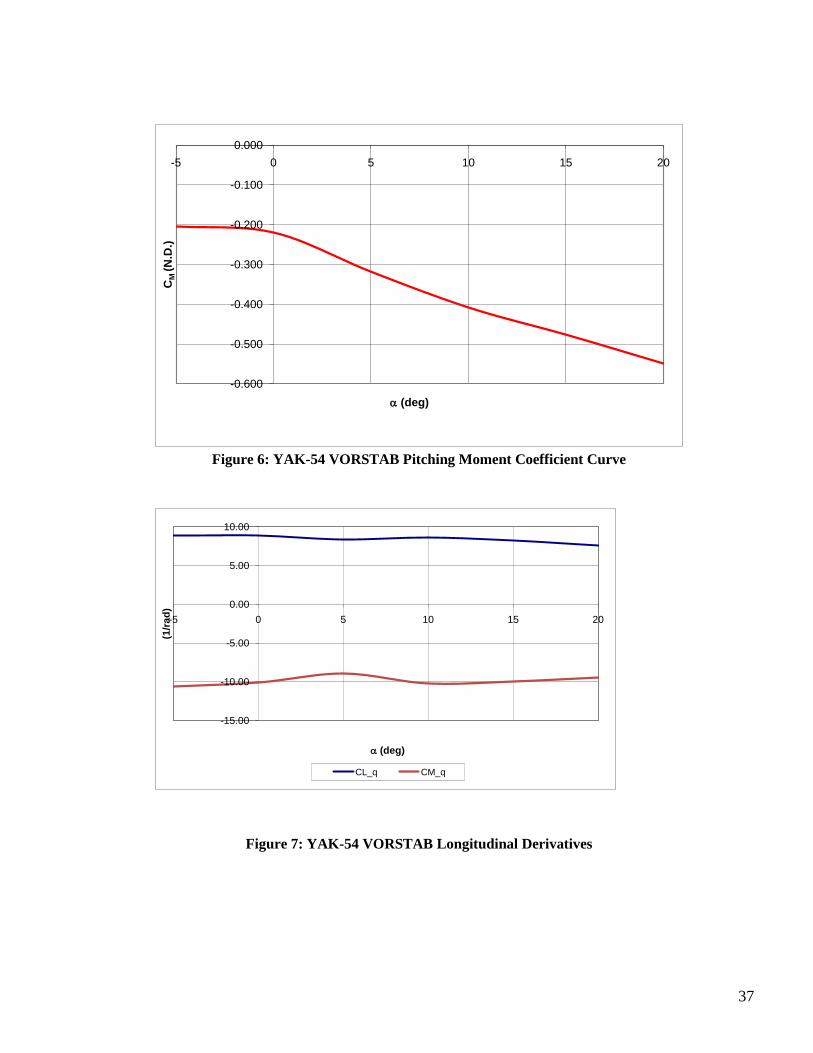
37

-0.600

-0.500

-0.400

-0.300

-0.200

-0.100

0.000

-5 0 5 10 15 20C

M (N

.D.)

(deg)

Figure 6: YAK-54 VORSTAB Pitching Moment Coefficient Curve

-15.00

-10.00

-5.00

0.00

5.00

10.00

-5 0 5 10 15 20

(1/r

ad

)

(deg)

CL_q CM_q

Figure 7: YAK-54 VORSTAB Longitudinal Derivatives

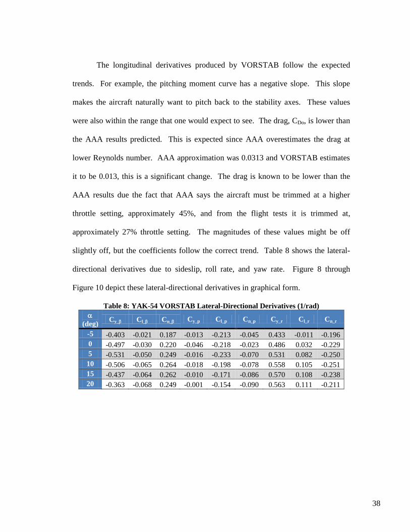
38

The longitudinal derivatives produced by VORSTAB follow the expected

trends. For example, the pitching moment curve has a negative slope. This slope

makes the aircraft naturally want to pitch back to the stability axes. These values

were also within the range that one would expect to see. The drag, CDo, is lower than

the AAA results predicted. This is expected since AAA overestimates the drag at

lower Reynolds number. AAA approximation was 0.0313 and VORSTAB estimates

it to be 0.013, this is a significant change. The drag is known to be lower than the

AAA results due the fact that AAA says the aircraft must be trimmed at a higher

throttle setting, approximately 45%, and from the flight tests it is trimmed at,

approximately 27% throttle setting. The magnitudes of these values might be off

slightly off, but the coefficients follow the correct trend. Table 8 shows the lateral-

directional derivatives due to sideslip, roll rate, and yaw rate. Figure 8 through

Figure 10 depict these lateral-directional derivatives in graphical form.

Table 8: YAK-54 VORSTAB Lateral-Directional Derivatives (1/rad)

(deg) Cy_ Cl_ Cn_ Cy_p Cl_p Cn_p Cy_r Cl_r Cn_r

-5 -0.403 -0.021 0.187 -0.013 -0.213 -0.045 0.433 -0.011 -0.196

0 -0.497 -0.030 0.220 -0.046 -0.218 -0.023 0.486 0.032 -0.229

5 -0.531 -0.050 0.249 -0.016 -0.233 -0.070 0.531 0.082 -0.250

10 -0.506 -0.065 0.264 -0.018 -0.198 -0.078 0.558 0.105 -0.251

15 -0.437 -0.064 0.262 -0.010 -0.171 -0.086 0.570 0.108 -0.238

20 -0.363 -0.068 0.249 -0.001 -0.154 -0.090 0.563 0.111 -0.211

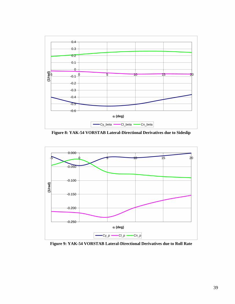
39

-0.6

-0.5

-0.4

-0.3

-0.2

-0.1

0

0.1

0.2

0.3

0.4

-5 0 5 10 15 20

(1/r

ad

)

(deg)

Cy_beta Cl_beta Cn_beta

Figure 8: YAK-54 VORSTAB Lateral-Directional Derivatives due to Sideslip

-0.250

-0.200

-0.150

-0.100

-0.050

0.000

-5 0 5 10 15 20

(1/r

ad

)

(deg)

Cy_p Cl_p Cn_p

Figure 9: YAK-54 VORSTAB Lateral-Directional Derivatives due to Roll Rate

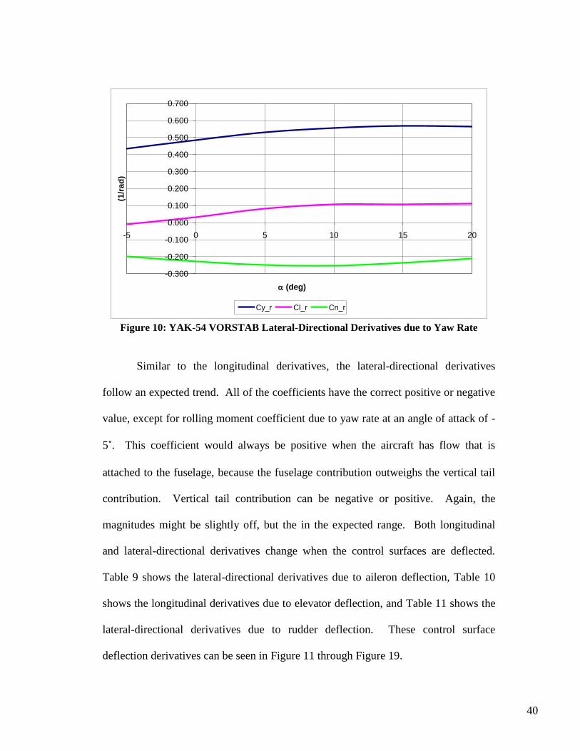
40

-0.300

-0.200

-0.100

0.000

0.100

0.200

0.300

0.400

0.500

0.600

0.700

-5 0 5 10 15 20

(1/r

ad

)

(deg)

Cy_r Cl_r Cn_r

Figure 10: YAK-54 VORSTAB Lateral-Directional Derivatives due to Yaw Rate

Similar to the longitudinal derivatives, the lateral-directional derivatives

follow an expected trend. All of the coefficients have the correct positive or negative

value, except for rolling moment coefficient due to yaw rate at an angle of attack of -

5˚. This coefficient would always be positive when the aircraft has flow that is

attached to the fuselage, because the fuselage contribution outweighs the vertical tail

contribution. Vertical tail contribution can be negative or positive. Again, the

magnitudes might be slightly off, but the in the expected range. Both longitudinal

and lateral-directional derivatives change when the control surfaces are deflected.

Table 9 shows the lateral-directional derivatives due to aileron deflection, Table 10

shows the longitudinal derivatives due to elevator deflection, and Table 11 shows the

lateral-directional derivatives due to rudder deflection. These control surface

deflection derivatives can be seen in Figure 11 through Figure 19.

41

Table 9: YAK-54 VORSTAB Lateral-Directional Due to Aileron Deflection (1/rad)

(deg) a Cy Cl Cn

0 -10 0.0009 -0.0240 -0.0054

5 -10 -0.0013 -0.0221 -0.0027

10 -10 -0.0041 -0.0243 0.0003

15 -10 -0.0077 -0.0224 0.0040

20 -10 -0.0103 -0.0176 0.0073

0 -5 -0.0054 -0.0120 0.0019

5 -5 -0.0070 -0.0110 0.0035

10 -5 -0.0083 -0.0121 0.0049

15 -5 -0.0093 -0.0111 0.0061

20 -5 -0.0099 -0.0087 0.0071

0 0 0.000 0.000 0.000

5 0 0.000 0.000 0.000

10 0 0.000 0.000 0.000

15 0 0.000 0.000 0.000

20 0 0.000 0.000 0.000

0 5 -0.0033 0.0121 0.0056

5 5 -0.0029 0.0110 0.0051

10 5 -0.0026 0.0121 0.0044

15 5 -0.0022 0.0110 0.0036

20 5 -0.0010 0.0086 0.0020

0 10 -0.0213 0.0244 0.0231

5 10 -0.0189 0.0221 0.0209

10 10 -0.0178 0.0242 0.0193

15 10 -0.0164 0.0219 0.0172

20 10 -0.0125 0.0171 0.0128

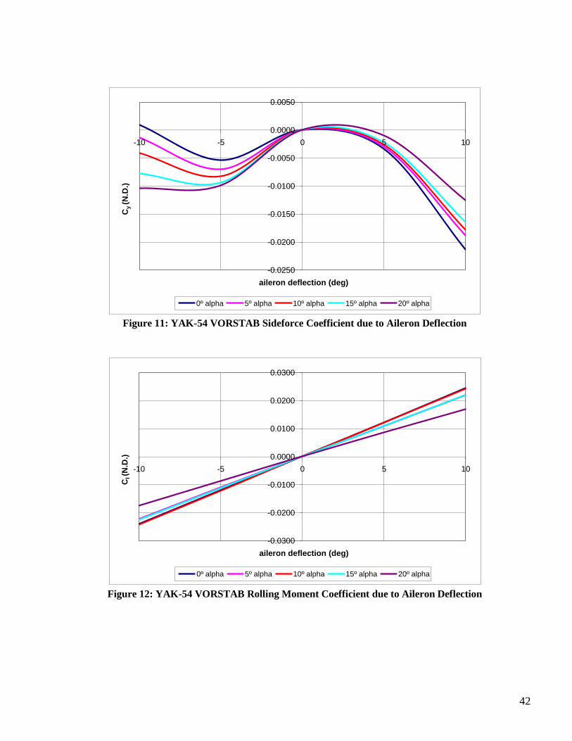
42

-0.0250

-0.0200

-0.0150

-0.0100

-0.0050

0.0000

0.0050

-10 -5 0 5 10

Cy (N

.D.)

aileron deflection (deg)

0º alpha 5º alpha 10º alpha 15º alpha 20º alpha

Figure 11: YAK-54 VORSTAB Sideforce Coefficient due to Aileron Deflection

-0.0300

-0.0200

-0.0100

0.0000

0.0100

0.0200

0.0300

-10 -5 0 5 10

Cl (N

.D.)



Figure 12: YAK-54 VORSTAB Rolling Moment Coefficient due to Aileron Deflection

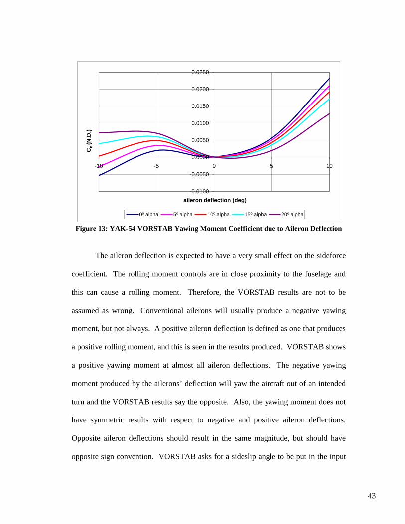
43

-0.0100

-0.0050

0.0000

0.0050

0.0100

0.0150

0.0200

0.0250

-10 -5 0 5 10

Cn

(N

.D.)



Figure 13: YAK-54 VORSTAB Yawing Moment Coefficient due to Aileron Deflection

The aileron deflection is expected to have a very small effect on the sideforce

coefficient. The rolling moment controls are in close proximity to the fuselage and

this can cause a rolling moment. Therefore, the VORSTAB results are not to be

assumed as wrong. Conventional ailerons will usually produce a negative yawing

moment, but not always. A positive aileron deflection is defined as one that produces

a positive rolling moment, and this is seen in the results produced. VORSTAB shows

a positive yawing moment at almost all aileron deflections. The negative yawing

moment produced by the ailerons‟ deflection will yaw the aircraft out of an intended

turn and the VORSTAB results say the opposite. Also, the yawing moment does not

have symmetric results with respect to negative and positive aileron deflections.

Opposite aileron deflections should result in the same magnitude, but should have

opposite sign convention. VORSTAB asks for a sideslip angle to be put in the input

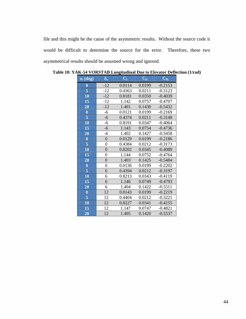
44

file and this might be the cause of the asymmetric results. Without the source code it

would be difficult to determine the source for the error. Therefore, these two

asymmetrical results should be assumed wrong and ignored.

Table 10: YAK-54 VORSTAB Longitudinal Due to Elevator Deflection (1/rad)

(deg) e CL CD CM

0 -12 0.0114 0.0199 -0.2153

5 -12 0.4363 0.0211 -0.3123

10 -12 0.8181 0.0350 -0.4039

15 -12 1.142 0.0757 -0.4707

20 -12 1.401 0.1430 -0.5432

0 -6 0.0121 0.0199 -0.2169

5 -6 0.4374 0.0211 -0.3148

10 -6 0.8191 0.0347 -0.4064

15 -6 1.143 0.0754 -0.4736

20 -6 1.402 0.1427 -0.5458

0 0 0.0129 0.0199 -0.2186

5 0 0.4384 0.0212 -0.3173

10 0 0.8202 0.0345 -0.4089

15 0 1.144 0.0752 -0.4764

20 0 1.403 0.1425 -0.5484

0 6 0.0136 0.0199 -0.2202

5 6 0.4394 0.0212 -0.3197

10 6 0.8213 0.0343 -0.4119

15 6 1.146 0.0749 -0.4793

20 6 1.404 0.1422 -0.5511

0 12 0.0143 0.0199 -0.2219

5 12 0.4404 0.0212 -0.3221

10 12 0.8227 0.0341 -0.4155

15 12 1.147 0.0747 -0.4821

20 12 1.405 0.1420 -0.5537

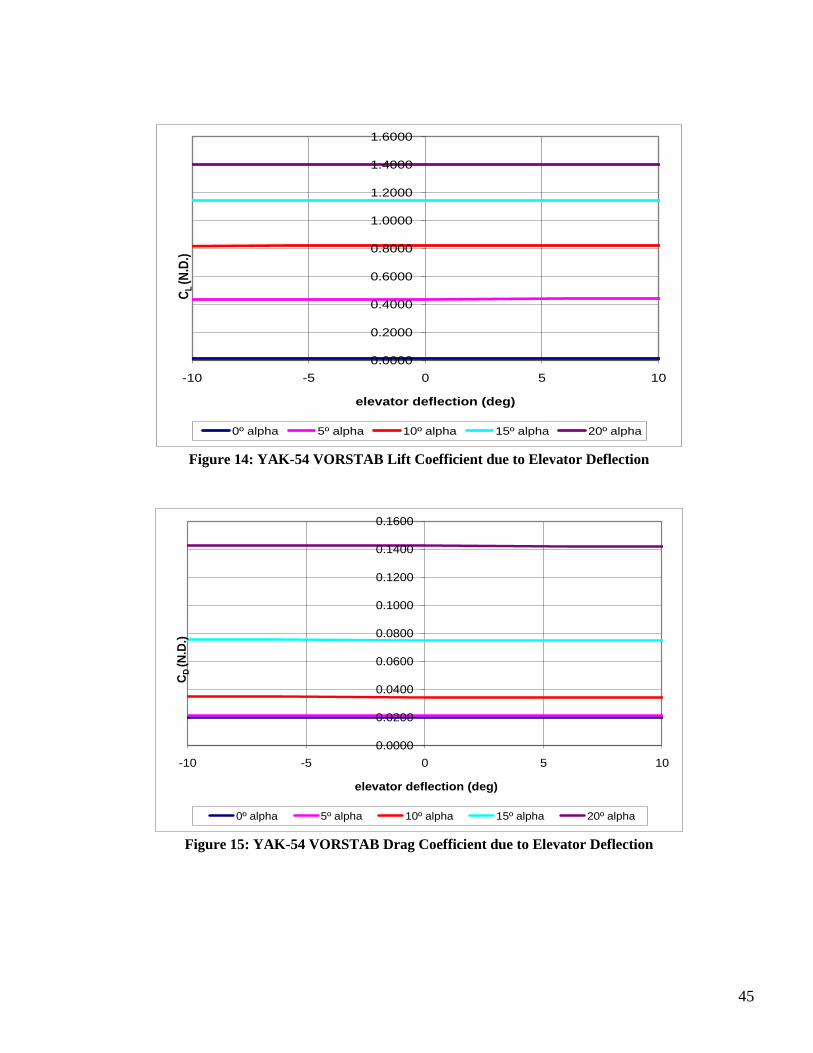
45

0.0000

0.2000

0.4000

0.6000

0.8000

1.0000

1.2000

1.4000

1.6000

-10 -5 0 5 10

CL

(N.D

.)

elevator deflection (deg)


Figure 14: YAK-54 VORSTAB Lift Coefficient due to Elevator Deflection

0.0000

0.0200

0.0400

0.0600

0.0800

0.1000

0.1200

0.1400

0.1600

-10 -5 0 5 10

CD

(N

.D.)



Figure 15: YAK-54 VORSTAB Drag Coefficient due to Elevator Deflection

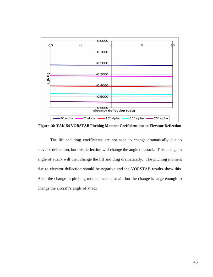
46

-0.6000

-0.5000

-0.4000

-0.3000

-0.2000

-0.1000

0.0000

-10 -5 0 5 10C

m (N

.D.)



Figure 16: YAK-54 VORSTAB Pitching Moment Coefficient due to Elevator Deflection

The lift and drag coefficients are not seen to change dramatically due to

elevator deflection, but this deflection will change the angle of attack. This change in

angle of attack will then change the lift and drag dramatically. The pitching moment

due to elevator deflection should be negative and the VORSTAB results show this.

Also, the change in pitching moment seems small, but the change is large enough to

change the aircraft‟s angle of attack.

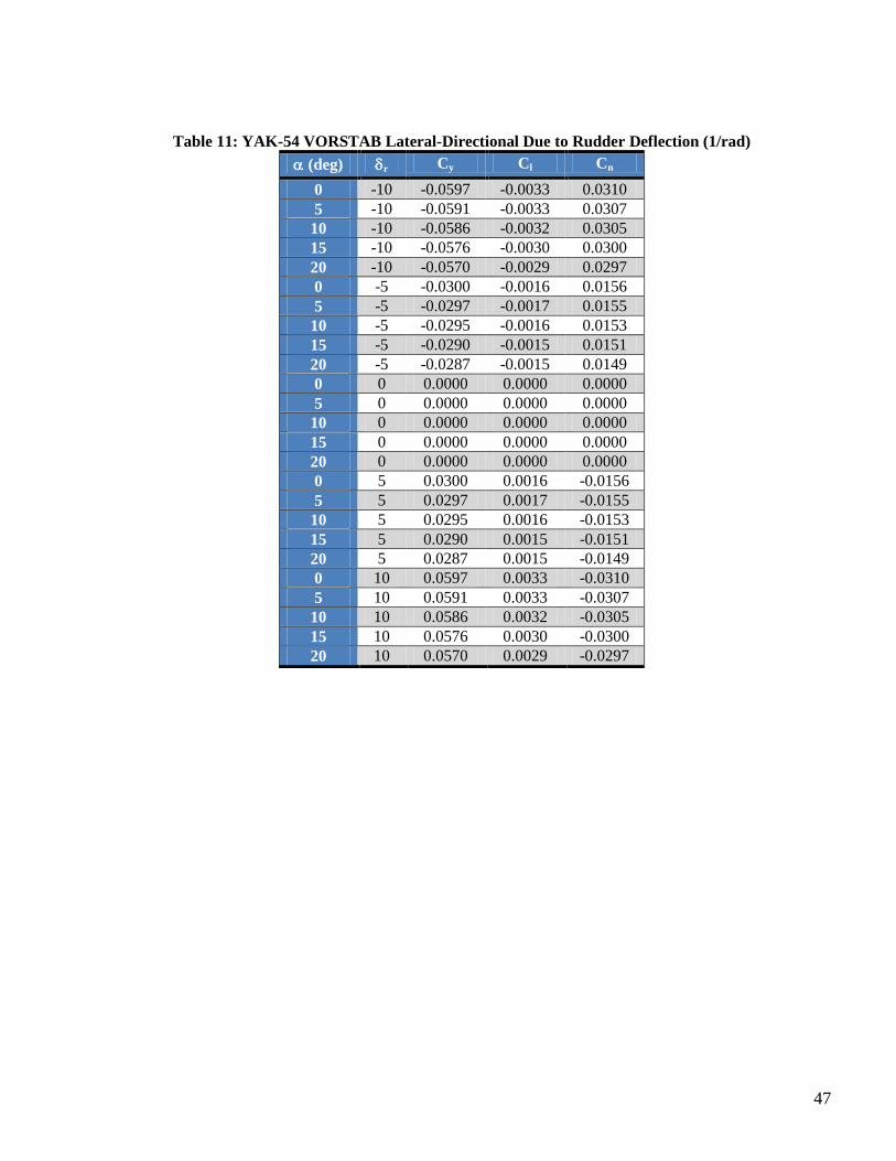
47

Table 11: YAK-54 VORSTAB Lateral-Directional Due to Rudder Deflection (1/rad)

(deg) r Cy Cl Cn

0 -10 -0.0597 -0.0033 0.0310

5 -10 -0.0591 -0.0033 0.0307

10 -10 -0.0586 -0.0032 0.0305

15 -10 -0.0576 -0.0030 0.0300

20 -10 -0.0570 -0.0029 0.0297

0 -5 -0.0300 -0.0016 0.0156

5 -5 -0.0297 -0.0017 0.0155

10 -5 -0.0295 -0.0016 0.0153

15 -5 -0.0290 -0.0015 0.0151

20 -5 -0.0287 -0.0015 0.0149

0 0 0.0000 0.0000 0.0000

5 0 0.0000 0.0000 0.0000

10 0 0.0000 0.0000 0.0000

15 0 0.0000 0.0000 0.0000

20 0 0.0000 0.0000 0.0000

0 5 0.0300 0.0016 -0.0156

5 5 0.0297 0.0017 -0.0155

10 5 0.0295 0.0016 -0.0153

15 5 0.0290 0.0015 -0.0151

20 5 0.0287 0.0015 -0.0149

0 10 0.0597 0.0033 -0.0310

5 10 0.0591 0.0033 -0.0307

10 10 0.0586 0.0032 -0.0305

15 10 0.0576 0.0030 -0.0300

20 10 0.0570 0.0029 -0.0297

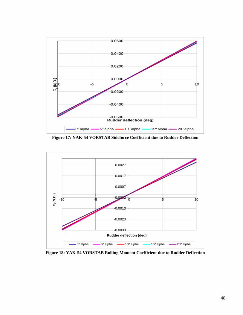
48

-0.0600

-0.0400

-0.0200

0.0000

0.0200

0.0400

0.0600

-10 -5 0 5 10

Cy (N

.D.)

Rudder deflection (deg)


Figure 17: YAK-54 VORSTAB Sideforce Coefficient due to Rudder Deflection

-0.0033

-0.0023

-0.0013

-0.0003

0.0007

0.0017

0.0027

-10 -5 0 5 10

Cl (N

.D.)



Figure 18: YAK-54 VORSTAB Rolling Moment Coefficient due to Rudder Deflection

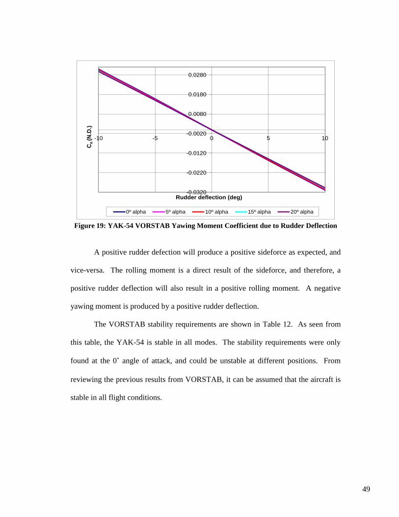
49

-0.0320

-0.0220

-0.0120

-0.0020

0.0080

0.0180

0.0280

-10 -5 0 5 10

Cn

(N

.D.)



Figure 19: YAK-54 VORSTAB Yawing Moment Coefficient due to Rudder Deflection

A positive rudder defection will produce a positive sideforce as expected, and

vice-versa. The rolling moment is a direct result of the sideforce, and therefore, a

positive rudder deflection will also result in a positive rolling moment. A negative

yawing moment is produced by a positive rudder deflection.

The VORSTAB stability requirements are shown in Table 12. As seen from

this table, the YAK-54 is stable in all modes. The stability requirements were only

found at the 0˚ angle of attack, and could be unstable at different positions. From

reviewing the previous results from VORSTAB, it can be assumed that the aircraft is

stable in all flight conditions.

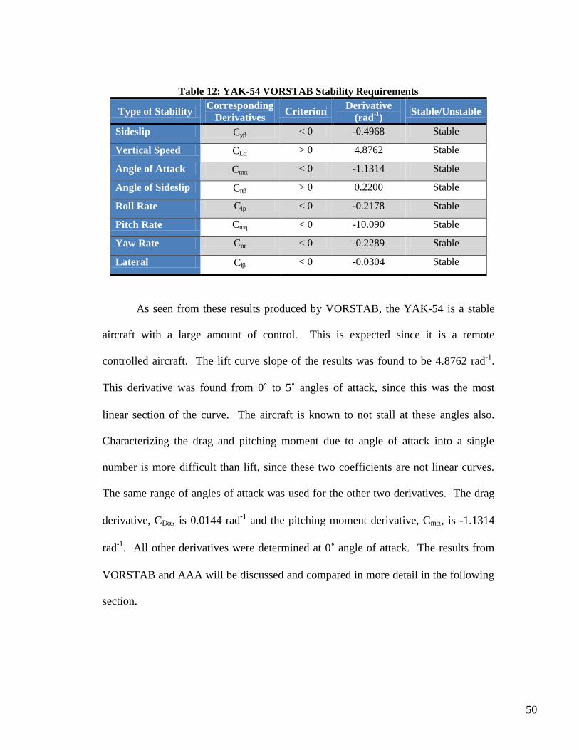
50

Table 12: YAK-54 VORSTAB Stability Requirements

Type of Stability Corresponding

Derivatives Criterion

Derivative

(rad-1

) Stable/Unstable




Angle of Sideslip Cn > 0 0.2200 Stable





As seen from these results produced by VORSTAB, the YAK-54 is a stable

aircraft with a large amount of control. This is expected since it is a remote

controlled aircraft. The lift curve slope of the results was found to be 4.8762 rad-1

.

This derivative was found from 0˚ to 5˚ angles of attack, since this was the most

linear section of the curve. The aircraft is known to not stall at these angles also.

Characterizing the drag and pitching moment due to angle of attack into a single

number is more difficult than lift, since these two coefficients are not linear curves.

The same range of angles of attack was used for the other two derivatives. The drag

derivative, CD, is 0.0144 rad-1

and the pitching moment derivative, Cm, is -1.1314

rad-1

. All other derivatives were determined at 0˚ angle of attack. The results from

VORSTAB and AAA will be discussed and compared in more detail in the following

section.

51

7.3 Method Comparison YAK-54

Both AAA and VORSTAB are considered as an accurate approximation for

the control derivatives. Using a computational fluid dynamic method such as

VORSTAB should produce results closer to that of the actual data than results from

DATCOM and AAA. As stated previously, the VORSTAB results were found over

an angle of attack range of 0˚ to 5˚. Table 13 shows the comparison data for the

YAK-54 for AAA and VORSTAB. The tuned AAA results were derived after

several flight tests were conducted, and the system identification warranted an

improved model. These turned values were taken from Ref [14] and explanation for

deriving them can be found there.

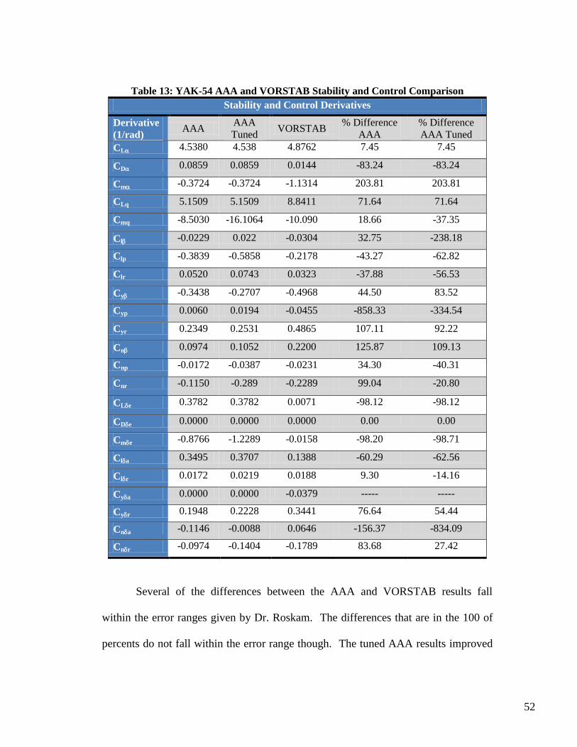
52

Table 13: YAK-54 AAA and VORSTAB Stability and Control Comparison

Stability and Control Derivatives

Derivative

(1/rad) AAA

AAA

Tuned VORSTAB

% Difference

AAA

% Difference

AAA Tuned

CL 4.5380 4.538 4.8762 7.45 7.45

CD 0.0859 0.0859 0.0144 -83.24 -83.24

Cm -0.3724 -0.3724 -1.1314 203.81 203.81

CLq 5.1509 5.1509 8.8411 71.64 71.64

Cmq -8.5030 -16.1064 -10.090 18.66 -37.35

Cl -0.0229 0.022 -0.0304 32.75 -238.18

Clp -0.3839 -0.5858 -0.2178 -43.27 -62.82

Clr 0.0520 0.0743 0.0323 -37.88 -56.53

Cy -0.3438 -0.2707 -0.4968 44.50 83.52

Cyp 0.0060 0.0194 -0.0455 -858.33 -334.54

Cyr 0.2349 0.2531 0.4865 107.11 92.22

Cn 0.0974 0.1052 0.2200 125.87 109.13

Cnp -0.0172 -0.0387 -0.0231 34.30 -40.31

Cnr -0.1150 -0.289 -0.2289 99.04 -20.80

CLe 0.3782 0.3782 0.0071 -98.12 -98.12

CDe 0.0000 0.0000 0.0000 0.00 0.00

Cme -0.8766 -1.2289 -0.0158 -98.20 -98.71

Cla 0.3495 0.3707 0.1388 -60.29 -62.56

Clr 0.0172 0.0219 0.0188 9.30 -14.16

Cya 0.0000 0.0000 -0.0379 ----- -----

Cyr 0.1948 0.2228 0.3441 76.64 54.44

Cna -0.1146 -0.0088 0.0646 -156.37 -834.09

Cnr -0.0974 -0.1404 -0.1789 83.68 27.42

Several of the differences between the AAA and VORSTAB results fall

within the error ranges given by Dr. Roskam. The differences that are in the 100 of

percents do not fall within the error range though. The tuned AAA results improved

53

in some cases and not in others. These derivatives, Cnr, Cnr, Cl, Cmq, and Cme were

tuned from the flight test and the others were taken from the AVL model. The tuned

yawing moment derivatives show an improvement in the VORSTAB results over

AAA. More flight tests need to be conducted and parameter system identification

need to be conducted to improve all of the derivatives.

Both methods show that the aircraft is stable. For stability and control

derivatives, there are typical ranges that can be expected, and through his vast

experience, Dr. Jan Roskam developed ranges for the control derivatives. These

ranges are for conventional aircraft, and the ranges are a function of Mach number.

Table 14 shows the Dr. Roskam, Ref. [1], typical ranges compared to the AAA and

VORSTAB results.

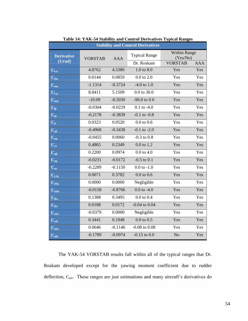
54

Table 14: YAK-54 Stability and Control Derivatives Typical Ranges


Derivative

(1/rad) VORSTAB AAA

Typical Range Within Range

(Yes/No)

Dr. Roskam VORSTAB AAA

CL 4.8762 4.5380 1.0 to 8.0 Yes Yes

CD 0.0144 0.0859 0.0 to 2.0 Yes Yes

Cm -1.1314 -0.3724 -4.0 to 1.0 Yes Yes

CLq 8.8411 5.1509 0.0 to 30.0 Yes Yes

Cmq -10.09 -8.5030 -90.0 to 0.0 Yes Yes

Cl -0.0304 -0.0229 0.1 to -4.0 Yes Yes

Clp -0.2178 -0.3839 -0.1 to -0.8 Yes Yes

Clr 0.0323 0.0520 0.0 to 0.6 Yes Yes

Cy -0.4968 -0.3438 -0.1 to -2.0 Yes Yes

Cyp -0.0455 0.0060 -0.3 to 0.8 Yes Yes

Cyr 0.4865 0.2349 0.0 to 1.2 Yes Yes

Cn 0.2200 0.0974 0.0 to 4.0 Yes Yes

Cnp -0.0231 -0.0172 -0.5 to 0.1 Yes Yes

Cnr -0.2289 -0.1150 0.0 to -1.0 Yes Yes

CLe 0.0071 0.3782 0.0 to 0.6 Yes Yes

CDe 0.0000 0.0000 Negligible Yes Yes

Cme -0.0158 -0.8766 0.0 to -4.0 Yes Yes

Cla 0.1388 0.3495 0.0 to 0.4 Yes Yes

Clr 0.0188 0.0172 -0.04 to 0.04 Yes Yes

Cya -0.0379 0.0000 Negligible Yes Yes

Cyr 0.3441 0.1948 0.0 to 0.5 Yes Yes

Cna 0.0646 -0.1146 -0.08 to 0.08 Yes Yes

Cnr -0.1789 -0.0974 -0.15 to 0.0 No Yes

The YAK-54 VORSTAB results fall within all of the typical ranges that Dr.

Roskam developed except for the yawing moment coefficient due to rudder

deflection, Cnr. These ranges are just estimations and many aircraft‟s derivatives do

55

not fall into the ranges. The ranges just give the designer an idea of things to expect.

Also, the sideforce moment coefficient due to aileron deflection, Cya, is not

negligible. This can happen when the rolling moment controls are in close proximity

to a vertical surface (fuselage or vertical tail). The ailerons, on the YAK-54, are in

close proximity to the fuselage, and this causes the coefficient to be a non-negligible

value. The AAA results all fall within the typical ranges. From these results, it is

concluded that both programs obtained valid results. These results should be

compared to the more flight test data to validate both software programs. A model

should be created with the new flight test data and then compared to the AAA and

VORSTAB results.

7.4 Linearized Model of the YAK-54

For the information and data on the state space model please refer to

Appendix B.

56

8 MantaHawk

The MantaHawk is a remote control aircraft designed at the University of

Kansas, by the AE 721 graduate design course in the fall 2009. The design team

consisted of Emily Arnold, Robert Burns, Dustin Grorud, Katrina Legursky, Rick

Riley, Dave Royer, and Jonathan Tom. This small UAV was developed in

conjunction with the CReSIS Meridian project. MantaHawk‟s size and weight were

well suited for a sea-born launch with a much shorter range than the other Meridian

Antarctic mission. The goal of the team was to help improve the current research

going on at the University of Kansas and within CReSIS itself.

After much was research conducted by the team, a wing-body configuration

was chosen as the most suitable configuration for the particular mission. The design

of the MantaHawk followed the Dr. Roskam method using AAA ,and AVL for some

of the stability and control derivatives that AAA did not produce. Class II design

resulted in an empty weight of 32 lbs for the vehicle with a design cruise speed of 70

kts. The vehicle had a payload capacity of 15 lbs plus 7 lbs of fuel. This aircraft was

a prototype and had its problems. Soon after take-off, the aircraft pitched downward

aggressively, and this caused the airplane to go into a nose dive. With post flight

analysis, the team determined that a negative pitching moment was much higher than

predicted and without pre-flight trim there was not enough control to fly. Figure 20

shows the MantaHawk designed by the AE 721 class, Ref [15]. The design and flight

test of the MantaHawk can be found in Ref [15].

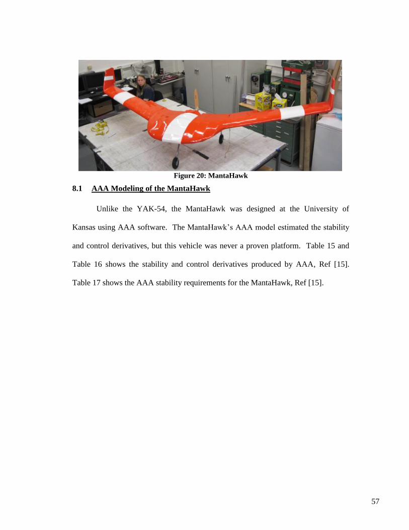
57

Figure 20: MantaHawk

8.1 AAA Modeling of the MantaHawk

Unlike the YAK-54, the MantaHawk was designed at the University of

Kansas using AAA software. The MantaHawk‟s AAA model estimated the stability

and control derivatives, but this vehicle was never a proven platform. Table 15 and

Table 16 shows the stability and control derivatives produced by AAA, Ref [15].

Table 17 shows the AAA stability requirements for the MantaHawk, Ref [15].

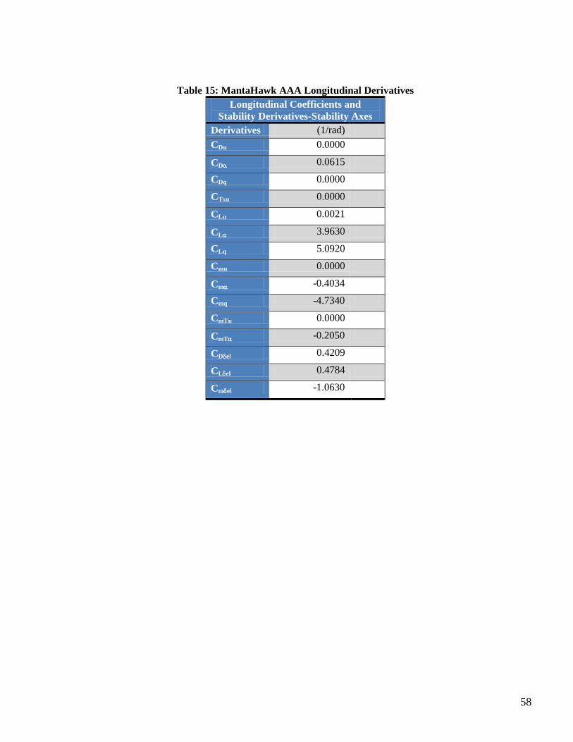
58

Table 15: MantaHawk AAA Longitudinal Derivatives

Longitudinal Coefficients and

Stability Derivatives-Stability Axes

Derivatives (1/rad)

CDu 0.0000

CD 0.0615

CDq 0.0000

CTxu 0.0000

CLu 0.0021

CL 3.9630

CLq 5.0920

Cmu 0.0000

Cm -0.4034

Cmq -4.7340

CmTu 0.0000

CmT -0.2050

CDel 0.4209

CLel 0.4784

Cmel -1.0630

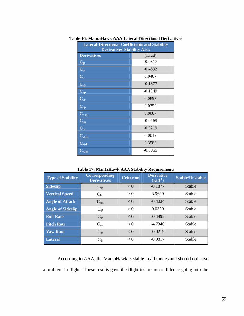
59

Table 16: MantaHawk AAA Lateral-Directional Derivatives

Lateral-Directional Coefficients and Stability


Derivatives (1/rad)

Cl -0.0817

Clp -0.4892

Clr 0.0407

Cy -0.1877

Cyp -0.1249

Cyr 0.0897

Cn 0.0359

CnT 0.0007

Cnp -0.0169

Cnr -0.0219

Cyel 0.0012

Clel 0.3588

Cnel -0.0055

Table 17: MantaHawk AAA Stability Requirements



Derivative

(rad-1

) Stable/Unstable









According to AAA, the MantaHawk is stable in all modes and should not have

a problem in flight. These results gave the flight test team confidence going into the

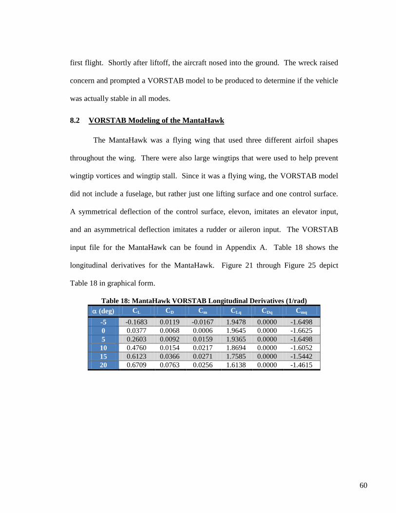
60

first flight. Shortly after liftoff, the aircraft nosed into the ground. The wreck raised

concern and prompted a VORSTAB model to be produced to determine if the vehicle

was actually stable in all modes.

8.2 VORSTAB Modeling of the MantaHawk

The MantaHawk was a flying wing that used three different airfoil shapes

throughout the wing. There were also large wingtips that were used to help prevent

wingtip vortices and wingtip stall. Since it was a flying wing, the VORSTAB model

did not include a fuselage, but rather just one lifting surface and one control surface.

A symmetrical deflection of the control surface, elevon, imitates an elevator input,

and an asymmetrical deflection imitates a rudder or aileron input. The VORSTAB

input file for the MantaHawk can be found in Appendix A. Table 18 shows the

longitudinal derivatives for the MantaHawk. Figure 21 through Figure 25 depict

Table 18 in graphical form.

Table 18: MantaHawk VORSTAB Longitudinal Derivatives (1/rad)

(deg) CL CD Cm CLq CDq Cmq

-5 -0.1683 0.0119 -0.0167 1.9478 0.0000 -1.6498

0 0.0377 0.0068 0.0006 1.9645 0.0000 -1.6625

5 0.2603 0.0092 0.0159 1.9365 0.0000 -1.6498

10 0.4760 0.0154 0.0217 1.8694 0.0000 -1.6052

15 0.6123 0.0366 0.0271 1.7585 0.0000 -1.5442

20 0.6709 0.0763 0.0256 1.6138 0.0000 -1.4615

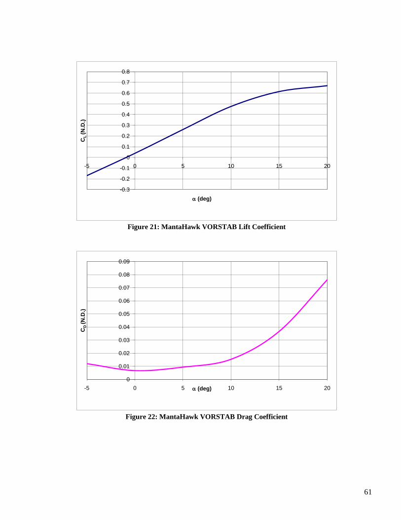
61

-0.3

-0.2

-0.1

0

0.1

0.2

0.3

0.4

0.5

0.6

0.7

0.8

-5 0 5 10 15 20

CL

(N

.D.)

(deg)

Figure 21: MantaHawk VORSTAB Lift Coefficient

0

0.01

0.02

0.03

0.04

0.05

0.06

0.07

0.08

0.09

-5 0 5 10 15 20

CD

(N

.D.)

(deg)

Figure 22: MantaHawk VORSTAB Drag Coefficient

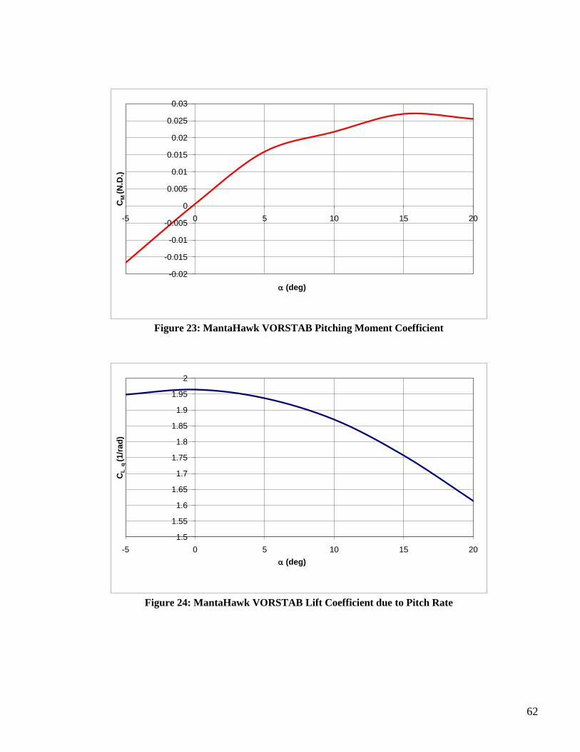
62

-0.02

-0.015

-0.01

-0.005

0

0.005

0.01

0.015

0.02

0.025

0.03

-5 0 5 10 15 20

CM

(N

.D.)

(deg)

Figure 23: MantaHawk VORSTAB Pitching Moment Coefficient

1.5

1.55

1.6

1.65

1.7

1.75

1.8

1.85

1.9

1.95

2

-5 0 5 10 15 20

CL

_q

(1/r

ad

)

(deg)

Figure 24: MantaHawk VORSTAB Lift Coefficient due to Pitch Rate

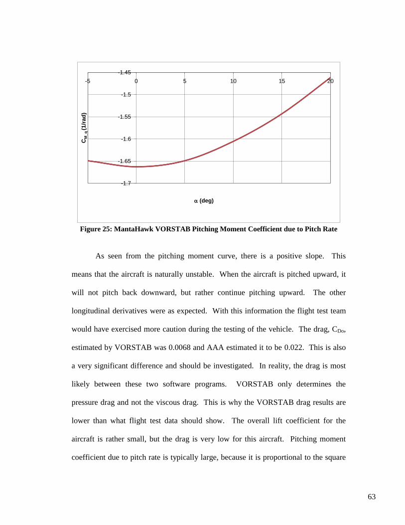
63

-1.7

-1.65

-1.6

-1.55

-1.5

-1.45

-5 0 5 10 15 20C

M_

q (1/r

ad

)

(deg)

Figure 25: MantaHawk VORSTAB Pitching Moment Coefficient due to Pitch Rate

As seen from the pitching moment curve, there is a positive slope. This

means that the aircraft is naturally unstable. When the aircraft is pitched upward, it

will not pitch back downward, but rather continue pitching upward. The other

longitudinal derivatives were as expected. With this information the flight test team

would have exercised more caution during the testing of the vehicle. The drag, CDo,

estimated by VORSTAB was 0.0068 and AAA estimated it to be 0.022. This is also

a very significant difference and should be investigated. In reality, the drag is most

likely between these two software programs. VORSTAB only determines the

pressure drag and not the viscous drag. This is why the VORSTAB drag results are

lower than what flight test data should show. The overall lift coefficient for the

aircraft is rather small, but the drag is very low for this aircraft. Pitching moment

coefficient due to pitch rate is typically large, because it is proportional to the square

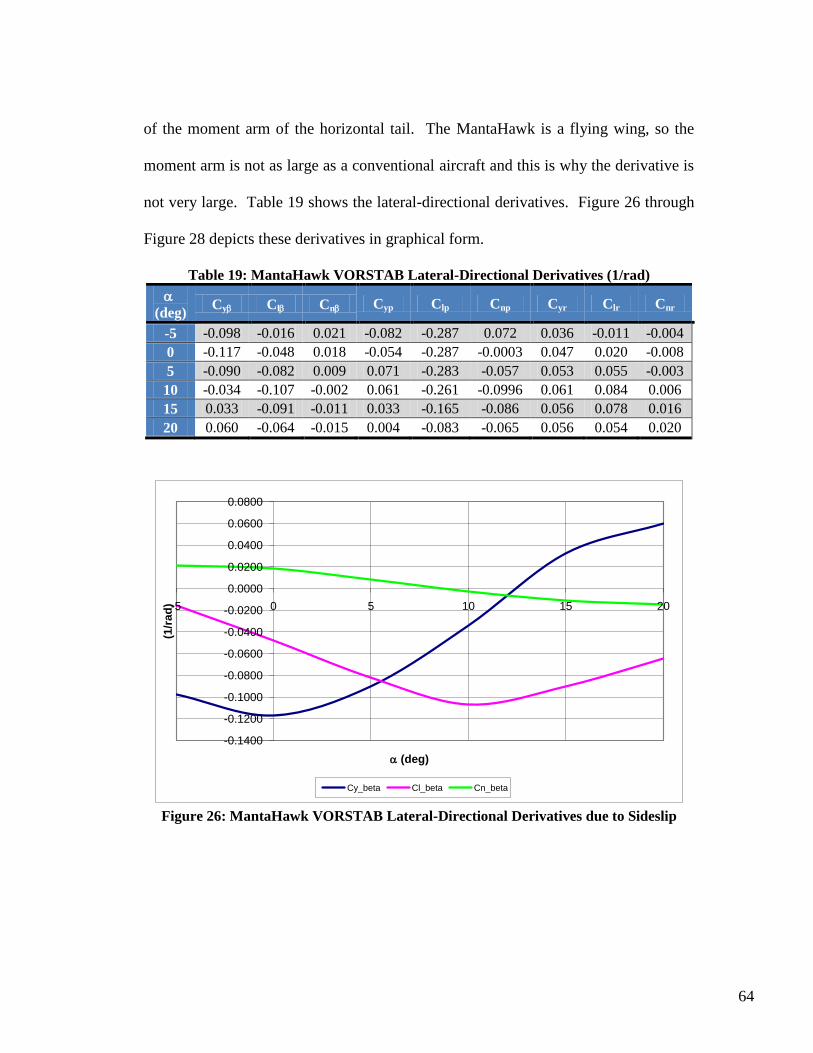
64

of the moment arm of the horizontal tail. The MantaHawk is a flying wing, so the

moment arm is not as large as a conventional aircraft and this is why the derivative is

not very large. Table 19 shows the lateral-directional derivatives. Figure 26 through

Figure 28 depicts these derivatives in graphical form.

Table 19: MantaHawk VORSTAB Lateral-Directional Derivatives (1/rad)

(deg) Cy Cl Cn Cyp Clp Cnp Cyr Clr Cnr

-5 -0.098 -0.016 0.021 -0.082 -0.287 0.072 0.036 -0.011 -0.004

0 -0.117 -0.048 0.018 -0.054 -0.287 -0.0003 0.047 0.020 -0.008

5 -0.090 -0.082 0.009 0.071 -0.283 -0.057 0.053 0.055 -0.003

10 -0.034 -0.107 -0.002 0.061 -0.261 -0.0996 0.061 0.084 0.006

15 0.033 -0.091 -0.011 0.033 -0.165 -0.086 0.056 0.078 0.016

20 0.060 -0.064 -0.015 0.004 -0.083 -0.065 0.056 0.054 0.020

-0.1400

-0.1200

-0.1000

-0.0800

-0.0600

-0.0400

-0.0200

0.0000

0.0200

0.0400

0.0600

0.0800

-5 0 5 10 15 20

(1/r

ad

)

(deg)

Cy_beta Cl_beta Cn_beta

Figure 26: MantaHawk VORSTAB Lateral-Directional Derivatives due to Sideslip

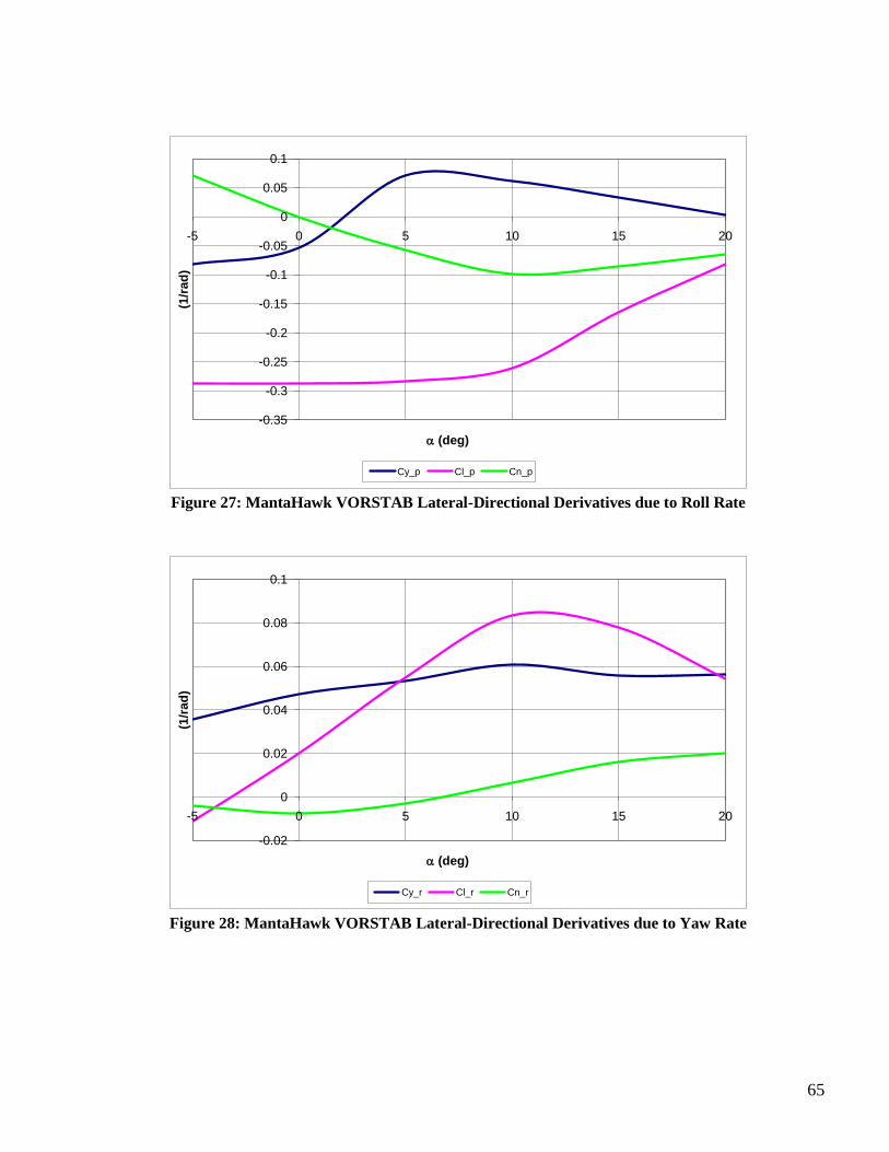
65

-0.35

-0.3

-0.25

-0.2

-0.15

-0.1

-0.05

0

0.05

0.1

-5 0 5 10 15 20

(1/r

ad

)

(deg)

Cy_p Cl_p Cn_p

Figure 27: MantaHawk VORSTAB Lateral-Directional Derivatives due to Roll Rate

-0.02

0

0.02

0.04

0.06

0.08

0.1

-5 0 5 10 15 20

(1/r

ad

)

(deg)

Cy_r Cl_r Cn_r

Figure 28: MantaHawk VORSTAB Lateral-Directional Derivatives due to Yaw Rate

66

At high angles of attack, aircrafts do not always follow the expected trends for

the derivatives. This is observed on several of these derivatives. The sideforce

coefficient due to sideslip is typically negative due to the defined positive angle of

sideslip. VORSTAB estimates that at high angles of attack this derivative becomes

positive. The yawing moment due to sideslip should be positive for the same reasons

as sideforce should be negative. This derivative becomes negative at high angles of

attack. Due to the definition of sideforce coefficient due to roll rate it would be

assumed that the derivative should be negative, but at high angles of attack the

moment arm will change signs. This will result in the derivative changing signs to

positive. It can be expected for the sign to change for the yawing moment derivative

due to roll rate as the angle of attack changes from positive to negative. The effect of

this derivative is rather small on the airplane dynamic stability, and since this is the

case the sign convention does not matter. Yawing moment coefficient due to yaw

rate changes signs due to the fact that as the angle of attack increase the moment arm

goes from positive to negative. All other derivatives were as expected.

With the control surfaces deflected, the longitudinal and lateral-directional

derivatives change. Table 20 shows the effects of an elevator input sent to the

elevons on the longitudinal derivatives. This type of input results in a symmetrical

deflection of the elevons. Table 21 shows the effects of the aileron or rudder input

sent to the elevons on the lateral directional derivatives. There is a resulting

asymmetrical deflection of the elevons. An asymmetrical deflection imitates an

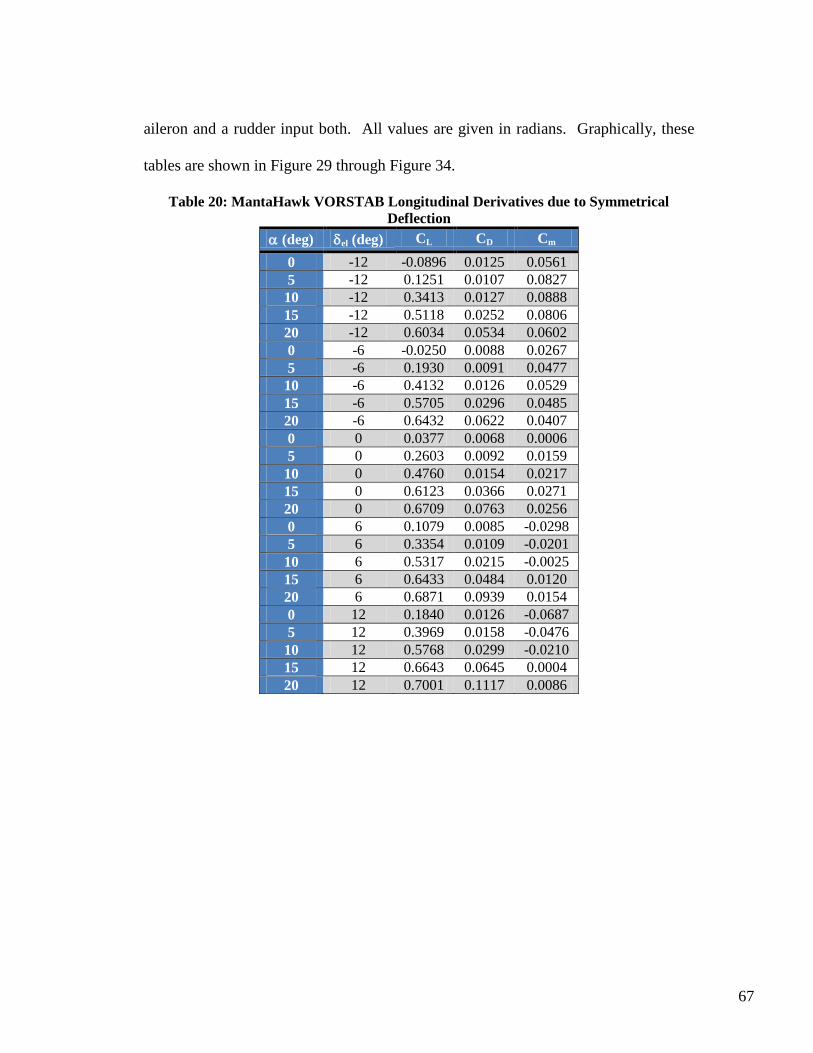
67

aileron and a rudder input both. All values are given in radians. Graphically, these

tables are shown in Figure 29 through Figure 34.

Table 20: MantaHawk VORSTAB Longitudinal Derivatives due to Symmetrical

Deflection

(deg) el (deg) CL CD Cm

0 -12 -0.0896 0.0125 0.0561

5 -12 0.1251 0.0107 0.0827

10 -12 0.3413 0.0127 0.0888

15 -12 0.5118 0.0252 0.0806

20 -12 0.6034 0.0534 0.0602

0 -6 -0.0250 0.0088 0.0267

5 -6 0.1930 0.0091 0.0477

10 -6 0.4132 0.0126 0.0529

15 -6 0.5705 0.0296 0.0485

20 -6 0.6432 0.0622 0.0407

0 0 0.0377 0.0068 0.0006

5 0 0.2603 0.0092 0.0159

10 0 0.4760 0.0154 0.0217

15 0 0.6123 0.0366 0.0271

20 0 0.6709 0.0763 0.0256

0 6 0.1079 0.0085 -0.0298

5 6 0.3354 0.0109 -0.0201

10 6 0.5317 0.0215 -0.0025

15 6 0.6433 0.0484 0.0120

20 6 0.6871 0.0939 0.0154

0 12 0.1840 0.0126 -0.0687

5 12 0.3969 0.0158 -0.0476

10 12 0.5768 0.0299 -0.0210

15 12 0.6643 0.0645 0.0004

20 12 0.7001 0.1117 0.0086

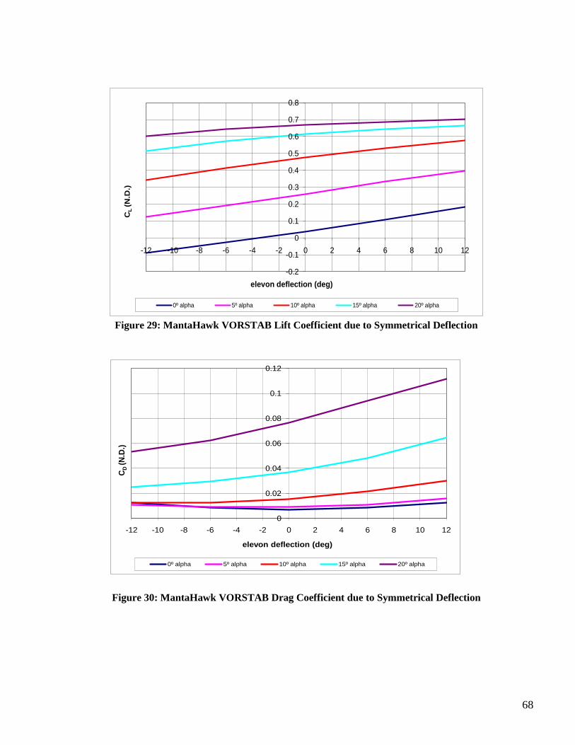
68

-0.2

-0.1

0

0.1

0.2

0.3

0.4

0.5

0.6

0.7

0.8

-12 -10 -8 -6 -4 -2 0 2 4 6 8 10 12

CL

(N

.D.)

elevon deflection (deg)


Figure 29: MantaHawk VORSTAB Lift Coefficient due to Symmetrical Deflection

0

0.02

0.04

0.06

0.08

0.1

0.12

-12 -10 -8 -6 -4 -2 0 2 4 6 8 10 12

CD

(N

.D.)



Figure 30: MantaHawk VORSTAB Drag Coefficient due to Symmetrical Deflection

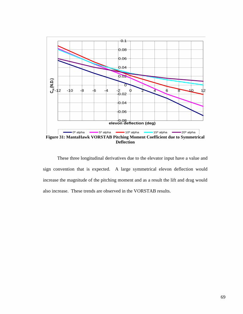
69

-0.08

-0.06

-0.04

-0.02

0

0.02

0.04

0.06

0.08

0.1

-12 -10 -8 -6 -4 -2 0 2 4 6 8 10 12Cm

(N.D

.)


0º alpha 5º alpha 10º alpha 15º alpha 20º alpha Figure 31: MantaHawk VORSTAB Pitching Moment Coefficient due to Symmetrical

Deflection

These three longitudinal derivatives due to the elevator input have a value and

sign convention that is expected. A large symmetrical elevon deflection would

increase the magnitude of the pitching moment and as a result the lift and drag would

also increase. These trends are observed in the VORSTAB results.

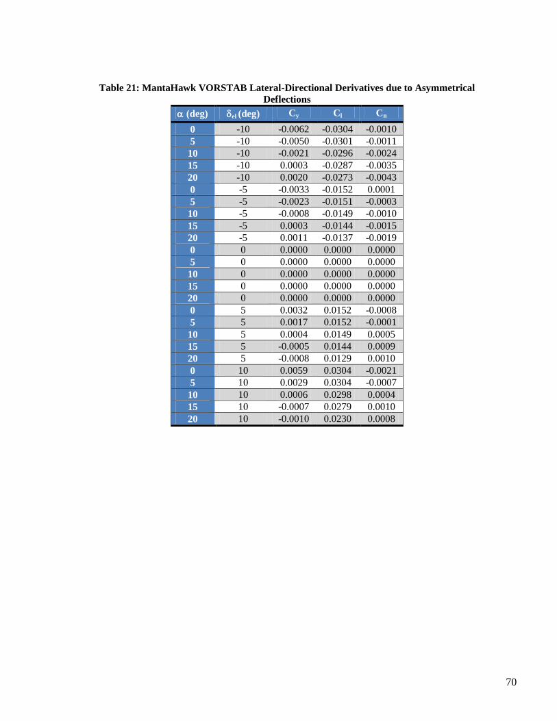
70

Table 21: MantaHawk VORSTAB Lateral-Directional Derivatives due to Asymmetrical

Deflections

(deg) el (deg) Cy Cl Cn

0 -10 -0.0062 -0.0304 -0.0010

5 -10 -0.0050 -0.0301 -0.0011

10 -10 -0.0021 -0.0296 -0.0024

15 -10 0.0003 -0.0287 -0.0035

20 -10 0.0020 -0.0273 -0.0043

0 -5 -0.0033 -0.0152 0.0001

5 -5 -0.0023 -0.0151 -0.0003

10 -5 -0.0008 -0.0149 -0.0010

15 -5 0.0003 -0.0144 -0.0015

20 -5 0.0011 -0.0137 -0.0019

0 0 0.0000 0.0000 0.0000

5 0 0.0000 0.0000 0.0000

10 0 0.0000 0.0000 0.0000

15 0 0.0000 0.0000 0.0000

20 0 0.0000 0.0000 0.0000

0 5 0.0032 0.0152 -0.0008

5 5 0.0017 0.0152 -0.0001

10 5 0.0004 0.0149 0.0005

15 5 -0.0005 0.0144 0.0009

20 5 -0.0008 0.0129 0.0010

0 10 0.0059 0.0304 -0.0021

5 10 0.0029 0.0304 -0.0007

10 10 0.0006 0.0298 0.0004

15 10 -0.0007 0.0279 0.0010

20 10 -0.0010 0.0230 0.0008

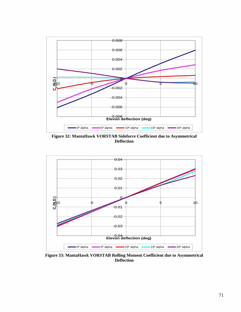
71

-0.008

-0.006

-0.004

-0.002

0

0.002

0.004

0.006

0.008

-10 -5 0 5 10

Cy (N

.D.)

Elevon deflection (deg)


Figure 32: MantaHawk VORSTAB Sideforce Coefficient due to Asymmetrical

Deflection

-0.04

-0.03

-0.02

-0.01

0

0.01

0.02

0.03

0.04

-10 -5 0 5 10

Cl (

N.D

.)



Figure 33: MantaHawk VORSTAB Rolling Moment Coefficient due to Asymmetrical

Deflection

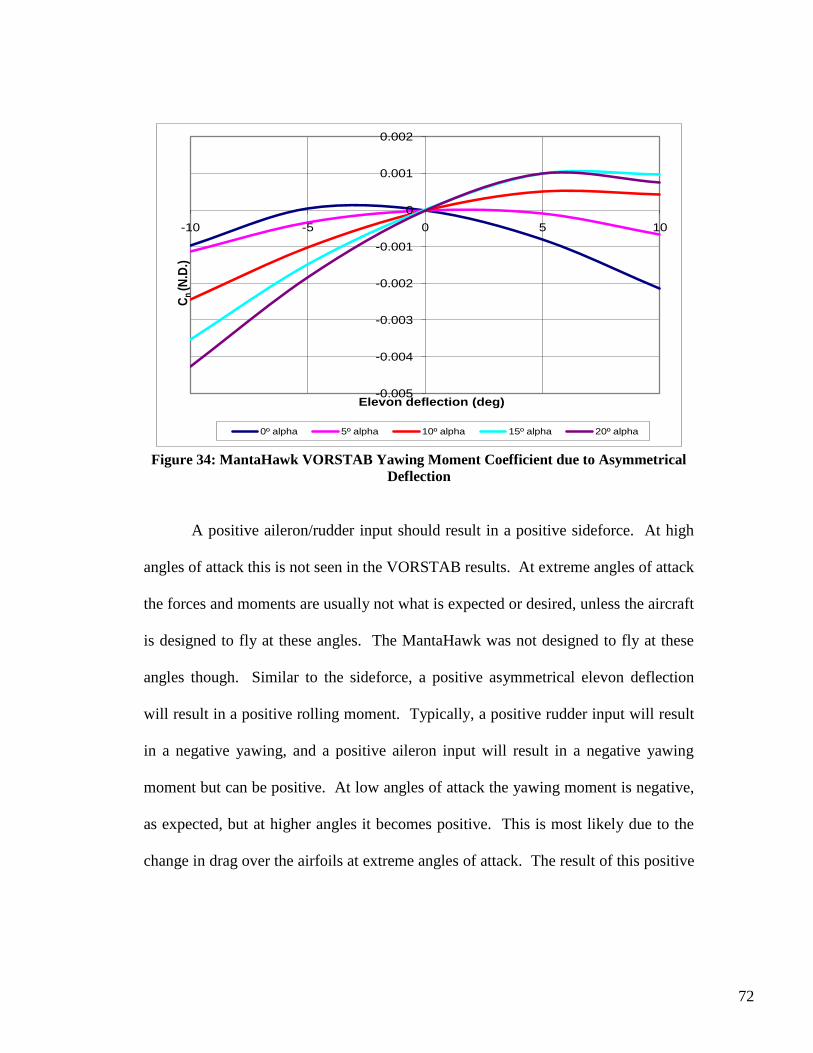
72

-0.005

-0.004

-0.003

-0.002

-0.001

0

0.001

0.002

-10 -5 0 5 10

Cn

(N.D

.)



Figure 34: MantaHawk VORSTAB Yawing Moment Coefficient due to Asymmetrical

Deflection

A positive aileron/rudder input should result in a positive sideforce. At high

angles of attack this is not seen in the VORSTAB results. At extreme angles of attack

the forces and moments are usually not what is expected or desired, unless the aircraft

is designed to fly at these angles. The MantaHawk was not designed to fly at these

angles though. Similar to the sideforce, a positive asymmetrical elevon deflection

will result in a positive rolling moment. Typically, a positive rudder input will result

in a negative yawing, and a positive aileron input will result in a negative yawing

moment but can be positive. At low angles of attack the yawing moment is negative,

as expected, but at higher angles it becomes positive. This is most likely due to the

change in drag over the airfoils at extreme angles of attack. The result of this positive

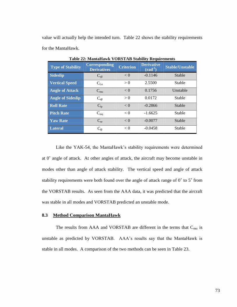
73

value will actually help the intended turn. Table 22 shows the stability requirements

for the MantaHawk.

Table 22: MantaHawk VORSTAB Stability Requirements



Derivative

(rad-1

) Stable/Unstable



Angle of Attack Cm < 0 0.1756 Unstable






Like the YAK-54, the MantaHawk‟s stability requirements were determined

at 0˚ angle of attack. At other angles of attack, the aircraft may become unstable in

modes other than angle of attack stability. The vertical speed and angle of attack

stability requirements were both found over the angle of attack range of 0˚ to 5˚ from

the VORSTAB results. As seen from the AAA data, it was predicted that the aircraft

was stable in all modes and VORSTAB predicted an unstable mode.

8.3 Method Comparison MantaHawk

The results from AAA and VORSTAB are different in the terms that Cm is

unstable as predicted by VORSTAB. AAA‟s results say that the MantaHawk is

stable in all modes. A comparison of the two methods can be seen in Table 23.

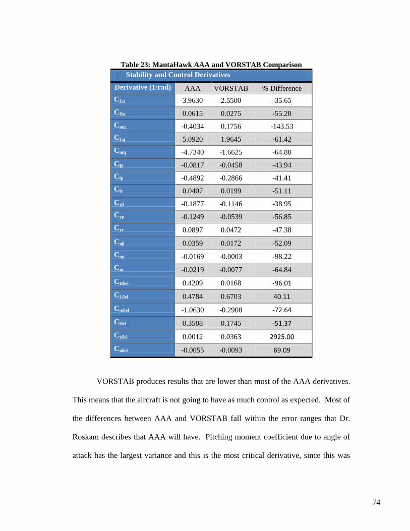
74

Table 23: MantaHawk AAA and VORSTAB Comparison


Derivative (1/rad) AAA VORSTAB % Difference

CL 3.9630 2.5500 -35.65

CD 0.0615 0.0275 -55.28

Cm -0.4034 0.1756 -143.53

CLq 5.0920 1.9645 -61.42

Cmq -4.7340 -1.6625 -64.88

Cl -0.0817 -0.0458 -43.94

Clp -0.4892 -0.2866 -41.41

Clr 0.0407 0.0199 -51.11

Cy -0.1877 -0.1146 -38.95

Cyp -0.1249 -0.0539 -56.85

Cyr 0.0897 0.0472 -47.38

Cn 0.0359 0.0172 -52.09

Cnp -0.0169 -0.0003 -98.22

Cnr -0.0219 -0.0077 -64.84

CDel 0.4209 0.0168 -96.01

CLel 0.4784 0.6703 40.11

Cmel -1.0630 -0.2908 -72.64

Clel 0.3588 0.1745 -51.37

Cyel 0.0012 0.0363 2925.00

Cnel -0.0055 -0.0093 69.09

VORSTAB produces results that are lower than most of the AAA derivatives.

This means that the aircraft is not going to have as much control as expected. Most of

the differences between AAA and VORSTAB fall within the error ranges that Dr.

Roskam describes that AAA will have. Pitching moment coefficient due to angle of

attack has the largest variance and this is the most critical derivative, since this was

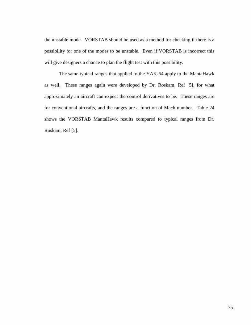
75

the unstable mode. VORSTAB should be used as a method for checking if there is a

possibility for one of the modes to be unstable. Even if VORSTAB is incorrect this

will give designers a chance to plan the flight test with this possibility.

The same typical ranges that applied to the YAK-54 apply to the MantaHawk

as well. These ranges again were developed by Dr. Roskam, Ref [5], for what

approximately an aircraft can expect the control derivatives to be. These ranges are

for conventional aircrafts, and the ranges are a function of Mach number. Table 24

shows the VORSTAB MantaHawk results compared to typical ranges from Dr.

Roskam, Ref [5].

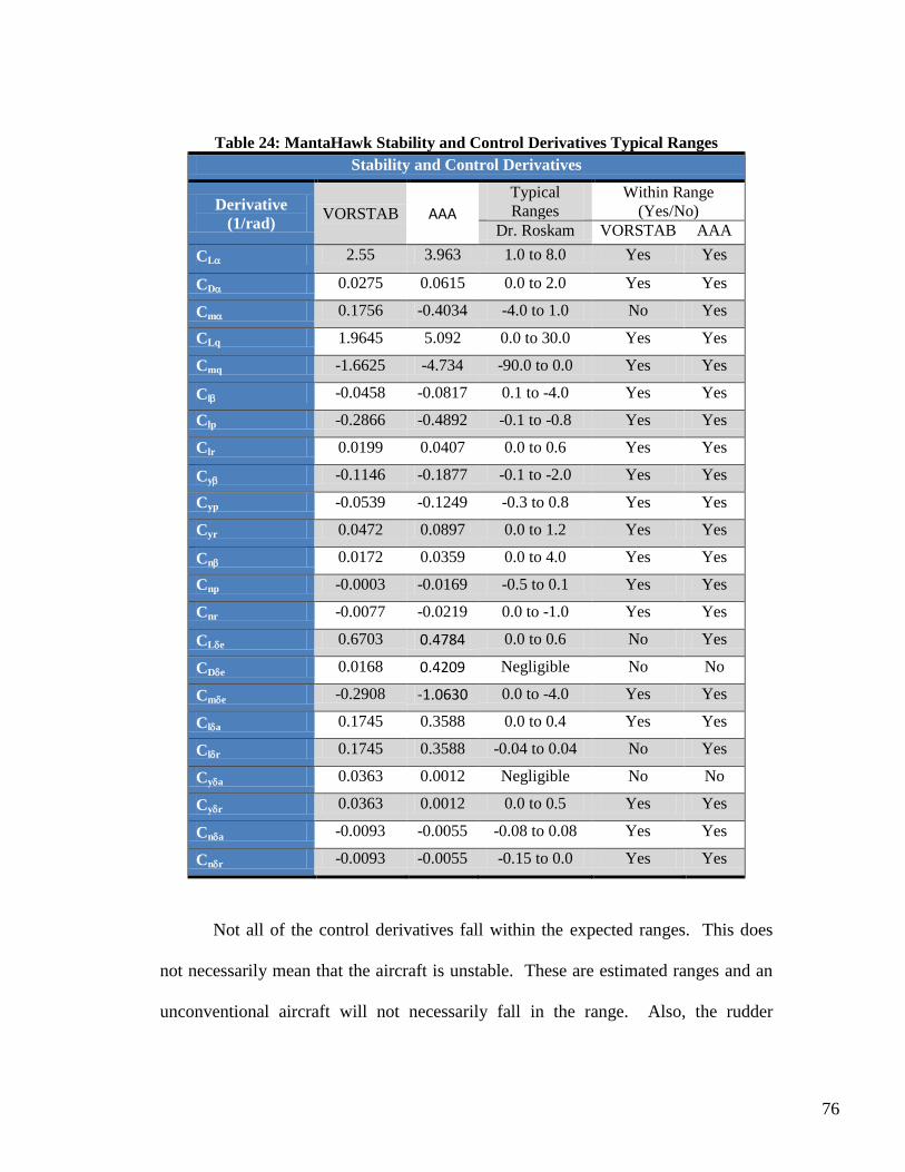
76

Table 24: MantaHawk Stability and Control Derivatives Typical Ranges


Derivative

(1/rad) VORSTAB AAA

Typical

Ranges

Within Range

(Yes/No)

Dr. Roskam VORSTAB AAA

CL 2.55 3.963 1.0 to 8.0 Yes Yes

CD 0.0275 0.0615 0.0 to 2.0 Yes Yes

Cm 0.1756 -0.4034 -4.0 to 1.0 No Yes

CLq 1.9645 5.092 0.0 to 30.0 Yes Yes

Cmq -1.6625 -4.734 -90.0 to 0.0 Yes Yes

Cl -0.0458 -0.0817 0.1 to -4.0 Yes Yes

Clp -0.2866 -0.4892 -0.1 to -0.8 Yes Yes

Clr 0.0199 0.0407 0.0 to 0.6 Yes Yes

Cy -0.1146 -0.1877 -0.1 to -2.0 Yes Yes

Cyp -0.0539 -0.1249 -0.3 to 0.8 Yes Yes

Cyr 0.0472 0.0897 0.0 to 1.2 Yes Yes

Cn 0.0172 0.0359 0.0 to 4.0 Yes Yes

Cnp -0.0003 -0.0169 -0.5 to 0.1 Yes Yes

Cnr -0.0077 -0.0219 0.0 to -1.0 Yes Yes

CLe 0.6703 0.4784 0.0 to 0.6 No Yes

CDe 0.0168 0.4209 Negligible No No

Cme -0.2908 -1.0630 0.0 to -4.0 Yes Yes

Cla 0.1745 0.3588 0.0 to 0.4 Yes Yes

Clr 0.1745 0.3588 -0.04 to 0.04 No Yes

Cya 0.0363 0.0012 Negligible No No

Cyr 0.0363 0.0012 0.0 to 0.5 Yes Yes

Cna -0.0093 -0.0055 -0.08 to 0.08 Yes Yes

Cnr -0.0093 -0.0055 -0.15 to 0.0 Yes Yes

Not all of the control derivatives fall within the expected ranges. This does

not necessarily mean that the aircraft is unstable. These are estimated ranges and an

unconventional aircraft will not necessarily fall in the range. Also, the rudder

77

deflection and aileron deflection control derivatives are the same because there is

only one input for those control surfaces. The input simulates both a rudder input and

an aileron input. This means that the control derivatives might fall into the range for

the rudder or aileron deflection, but not the other deflection. For example, the rolling

moment coefficient due to aileron deflection falls into the typical range Dr. Roskam

gives, but it does not fall into the typical range for the rudder deflection. The drag

coefficient due to elevator deflection is usually ignored. Therefore, there is no cause

for alarm that there is an increase in drag when the control surfaces are deflected. As

stated earlier, the MantaHawk is unstable in the pitching mode, and this is observed

since the pitching moment coefficient due to change in angle of attack, Cm, does not

fall into the typical range Dr. Roskam describes.

8.4 Linearized Model of the MantaHawk

For the information and data on the state space model please refer to

Appendix B.

78

9 Meridian UAV

The Center for Remote Sensing of Ice Sheets (CReSIS) is a science and

technology center established by the National Science Foundation (NSF) in 2005.

The foundation has the mission of developing new technologies and computer models

to measure and predict the response of sea level change to the mass balance of ice

sheets in Greenland and Antarctica. CReSIS is developing sophisticated sensors and

a long-duration un-inhabitant aerial vehicle (UAV), called the Meridian.

The KUAE, in close collaboration with national and international partners, has

designed and developed the Meridian UAV for the Center for Remote Sensing of Ice

Sheets (CReSIS). The Meridian has a gross takeoff weight of 1,100 lbs, a wingspan

of 26.4 ft, and a range of 950 nautical miles. Vehicle cruise speed is 100-120 kts,

endurance exceeds 9 hours, and available payload exceeds 120 lbs and 300W

consumed power. As such, this is an extraordinarily valuable scientific research

platform, since most civilian UAV research currently limits payloads to a few pounds

and a fraction of the power. Added benefits of greater than two cubic feet of payload

volume and eight wing hard points provide a sensor platform with little competition.

This data was taken from Ref [16]. Table 25 shows some of the important salient

characteristics and Figure 35 shows the design of the Meridian UAV both from Ref

[17]. Information about the design on the Meridian can also be found in Ref [17].

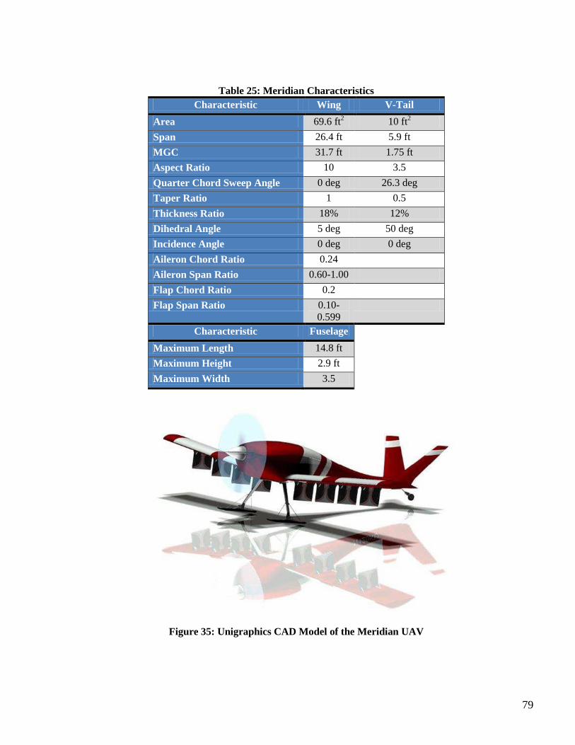
79

Table 25: Meridian Characteristics

Characteristic Wing V-Tail

Area 69.6 ft2 10 ft

2

Span 26.4 ft 5.9 ft

MGC 31.7 ft 1.75 ft

Aspect Ratio 10 3.5

Quarter Chord Sweep Angle 0 deg 26.3 deg

Taper Ratio 1 0.5

Thickness Ratio 18% 12%

Dihedral Angle 5 deg 50 deg

Incidence Angle 0 deg 0 deg

Aileron Chord Ratio 0.24

Aileron Span Ratio 0.60-1.00

Flap Chord Ratio 0.2

Flap Span Ratio 0.10-

0.599

Characteristic Fuselage

Maximum Length 14.8 ft

Maximum Height 2.9 ft

Maximum Width 3.5

Figure 35: Unigraphics CAD Model of the Meridian UAV

80

The design of the Meridian was completed using AAA and Dr. Roskam‟s

method. The AAA software was also used to find the stability and control derivatives

of the Meridian. The tail of the Meridian is unconventional and uses a v-tail. It is

also a fully moving tail.

9.1 AAA Modeling of the Meridian

Similar to the YAK-54 and MantaHawk, the AAA file produced stability and

control derivatives for the Meridian UAV. The longitudinal derivatives are found in

Table 26 and the lateral-directional derivatives are found in Table 27, both Ref [18].

As seen in Table 28 the aircraft is found to be stable in all modes.

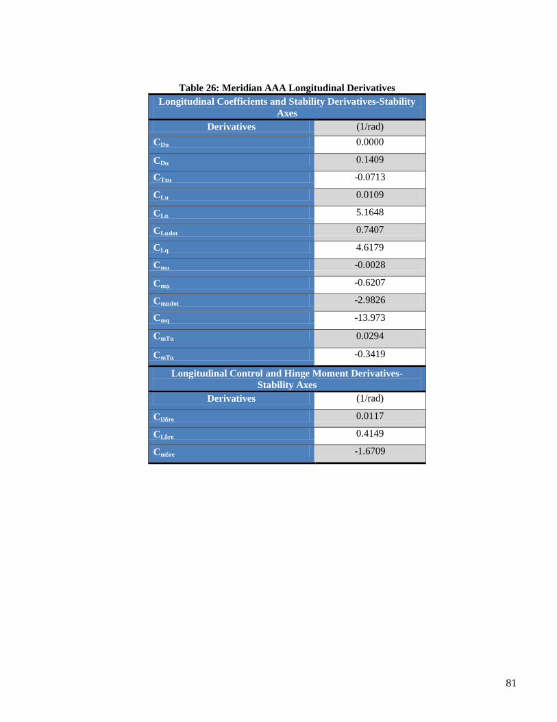
81

Table 26: Meridian AAA Longitudinal Derivatives

Longitudinal Coefficients and Stability Derivatives-Stability

Axes

Derivatives (1/rad)

CDu 0.0000

CD 0.1409

CTxu -0.0713

CLu 0.0109

CL 5.1648

CLdot 0.7407

CLq 4.6179

Cmu -0.0028

Cm -0.6207

Cmdot -2.9826

Cmq -13.973

CmTu 0.0294

CmT -0.3419

Longitudinal Control and Hinge Moment Derivatives-

Stability Axes

Derivatives (1/rad)

CDre 0.0117

CLre 0.4149

Cmre -1.6709

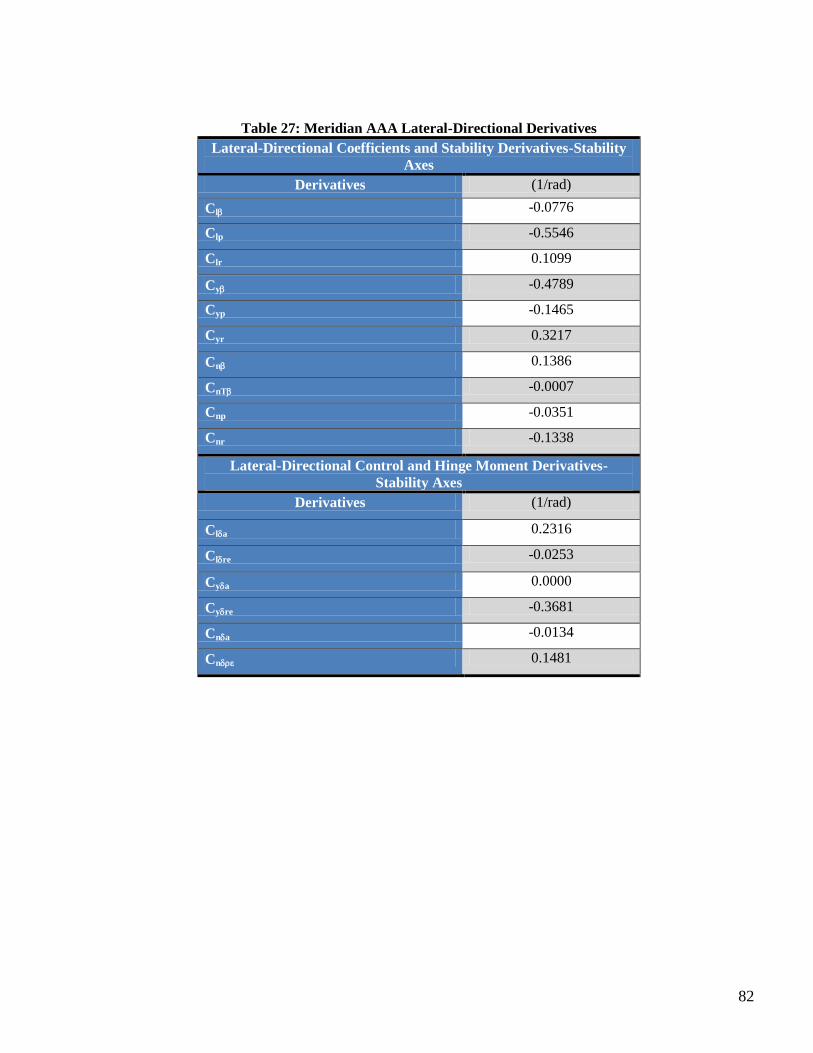
82

Table 27: Meridian AAA Lateral-Directional Derivatives

Lateral-Directional Coefficients and Stability Derivatives-Stability

Axes

Derivatives (1/rad)

Cl -0.0776

Clp -0.5546

Clr 0.1099

Cy -0.4789

Cyp -0.1465

Cyr 0.3217

Cn 0.1386

CnT -0.0007

Cnp -0.0351

Cnr -0.1338

Lateral-Directional Control and Hinge Moment Derivatives-

Stability Axes

Derivatives (1/rad)

Cla 0.2316

Clre -0.0253

Cya 0.0000

Cyre -0.3681

Cna -0.0134

Cn 0.1481

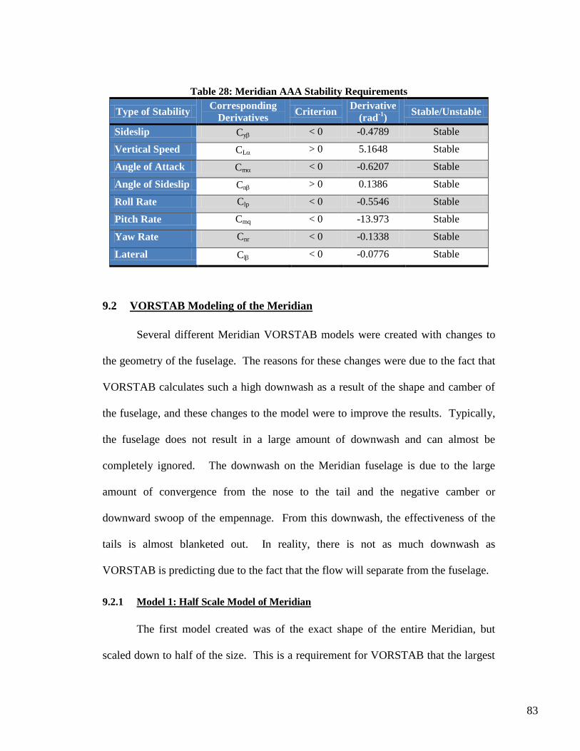
83

Table 28: Meridian AAA Stability Requirements



Derivative

(rad-1

) Stable/Unstable









9.2 VORSTAB Modeling of the Meridian

Several different Meridian VORSTAB models were created with changes to

the geometry of the fuselage. The reasons for these changes were due to the fact that

VORSTAB calculates such a high downwash as a result of the shape and camber of

the fuselage, and these changes to the model were to improve the results. Typically,

the fuselage does not result in a large amount of downwash and can almost be

completely ignored. The downwash on the Meridian fuselage is due to the large

amount of convergence from the nose to the tail and the negative camber or

downward swoop of the empennage. From this downwash, the effectiveness of the

tails is almost blanketed out. In reality, there is not as much downwash as

VORSTAB is predicting due to the fact that the flow will separate from the fuselage.

9.2.1 Model 1: Half Scale Model of Meridian

The first model created was of the exact shape of the entire Meridian, but

scaled down to half of the size. This is a requirement for VORSTAB that the largest

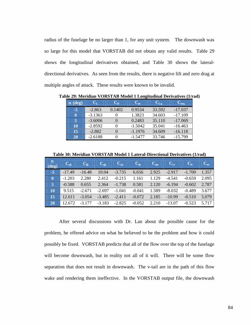
84

radius of the fuselage be no larger than 1, for any unit system. The downwash was

so large for this model that VORSTAB did not obtain any valid results. Table 29

shows the longitudinal derivatives obtained, and Table 30 shows the lateral-

directional derivatives. As seen from the results, there is negative lift and zero drag at

multiple angles of attack. These results were known to be invalid.

Table 29: Meridian VORSTAB Model 1 Longitudinal Derivatives (1/rad)

(deg) CL CD Cm CLq Cmq

-5 -2.863 0.1402 0.9534 33.592 -17.037

0 -3.1363 0 1.3823 34.603 -17.109

5 -3.6006 0 0.2483 35.110 -17.069

10 -2.8592 0 -1.5042 35.041 -16.463

15 -2.882 0 -1.1976 34.609 -16.118

20 -2.6188 0 -1.5477 33.746 -15.799

Table 30: Meridian VORSTAB Model 1 Lateral-Directional Derivatives (1/rad)


-5 -17.49 -16.48 10.04 -3.735 6.656 2.925 -2.917 -1.700 1.357

0 -1.203 2.280 2.412 -0.215 1.161 1.129 -4.541 -0.659 2.095

5 -0.588 0.655 2.364 -1.738 0.581 2.120 -6.194 -0.602 2.787

10 9.515 -2.671 -2.697 -1.041 -0.041 1.589 -8.032 -0.489 3.677

15 12.611 -3.054 -3.485 -2.411 -0.072 2.185 -10.99 -0.510 5.079

20 12.672 -3.177 -3.183 -2.825 -0.052 2.210 -13.07 -0.523 5.717

After several discussions with Dr. Lan about the possible cause for the

problem, he offered advice on what he believed to be the problem and how it could

possibly be fixed. VORSTAB predicts that all of the flow over the top of the fuselage

will become downwash, but in reality not all of it will. There will be some flow

separation that does not result in downwash. The v-tail are in the path of this flow

wake and rendering them ineffective. In the VORSTAB output file, the downwash

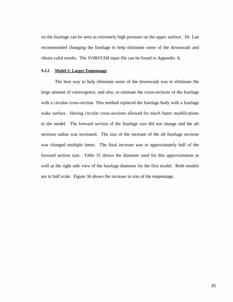
85

on the fuselage can be seen as extremely high pressure on the upper surface. Dr. Lan

recommended changing the fuselage to help eliminate some of the downwash and

obtain valid results. The VORSTAB input file can be found in Appendix A.

9.2.2 Model 2: Larger Empennage

The best way to help eliminate some of the downwash was to eliminate the

large amount of convergence, and also, to estimate the cross-sections of the fuselage

with a circular cross-section. This method replaced the fuselage body with a fuselage

wake surface. Having circular cross-sections allowed for much faster modifications

to the model. The forward section of the fuselage size did not change and the aft

sections radius was increased. The size of the increase of the aft fuselage sections

was changed multiple times. The final increase was to approximately half of the

forward section size. Table 31 shows the diameter used for this approximation as

well as the right side view of the fuselage diameter for the first model. Both models

are to half scale. Figure 36 shows the increase in size of the empennage.

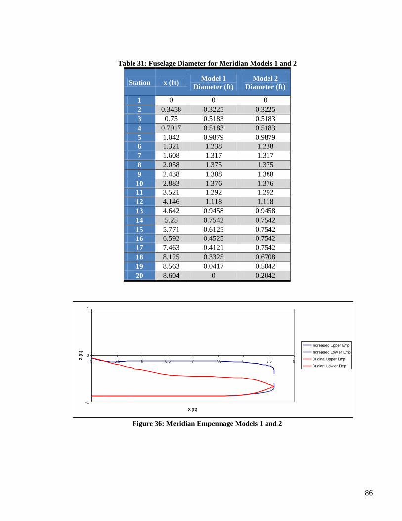
86

Table 31: Fuselage Diameter for Meridian Models 1 and 2

Station x (ft) Model 1

Diameter (ft)

Model 2

Diameter (ft)

1 0 0 0

2 0.3458 0.3225 0.3225

3 0.75 0.5183 0.5183

4 0.7917 0.5183 0.5183

5 1.042 0.9879 0.9879

6 1.321 1.238 1.238

7 1.608 1.317 1.317

8 2.058 1.375 1.375

9 2.438 1.388 1.388

10 2.883 1.376 1.376

11 3.521 1.292 1.292

12 4.146 1.118 1.118

13 4.642 0.9458 0.9458

14 5.25 0.7542 0.7542

15 5.771 0.6125 0.7542

16 6.592 0.4525 0.7542

17 7.463 0.4121 0.7542

18 8.125 0.3325 0.6708

19 8.563 0.0417 0.5042

20 8.604 0 0.2042

-1

0

1

5 5.5 6 6.5 7 7.5 8 8.5 9

X (ft)

Z (

ft)

Increased Upper Emp

Increased Low er Emp

Original Upper Emp

Origianl Low er Emp

Figure 36: Meridian Empennage Models 1 and 2

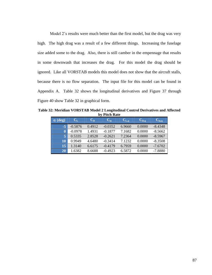
87

Model 2‟s results were much better than the first model, but the drag was very

high. The high drag was a result of a few different things. Increasing the fuselage

size added some to the drag. Also, there is still camber in the empennage that results

in some downwash that increases the drag. For this model the drag should be

ignored. Like all VORSTAB models this model does not show that the aircraft stalls,

because there is no flow separation. The input file for this model can be found in

Appendix A. Table 32 shows the longitudinal derivatives and Figure 37 through

Figure 40 show Table 32 in graphical form.

Table 32: Meridian VORSTAB Model 2 Longitudinal Control Derivatives and Affected

by Pitch Rate

(deg) CL CD Cm CL,q CD,q Cm,q

-5 -0.5876 0.4912 -0.0352 6.9660 0.0000 -8.4348

0 -0.0978 1.4931 -0.1877 7.1682 0.0000 -8.5662

5 0.5335 2.8528 -0.2621 7.2364 0.0000 -8.5967

10 0.9949 4.6480 -0.3414 7.1232 0.0000 -8.3508

15 1.3140 6.6175 -0.4179 6.7959 0.0000 -7.6702

20 1.6382 8.6688 -0.4923 6.5872 0.0000 -7.8880

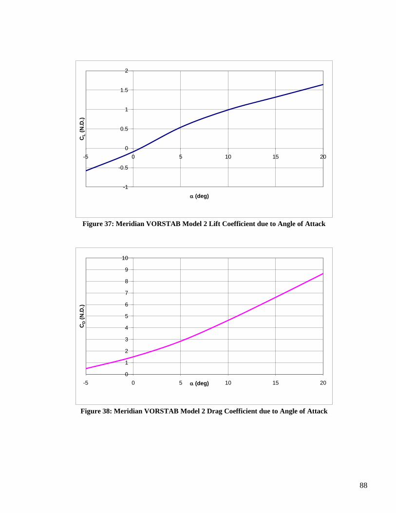
88

-1

-0.5

0

0.5

1

1.5

2

-5 0 5 10 15 20

CL

(N.D

.)

(deg)

Figure 37: Meridian VORSTAB Model 2 Lift Coefficient due to Angle of Attack

0

1

2

3

4

5

6

7

8

9

10

-5 0 5 10 15 20

CD

(N.D

.)

(deg)

Figure 38: Meridian VORSTAB Model 2 Drag Coefficient due to Angle of Attack

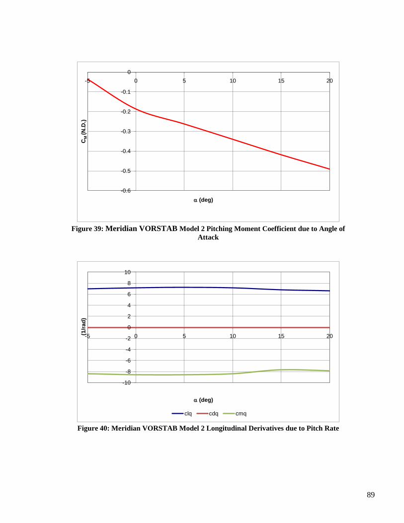
89

-0.6

-0.5

-0.4

-0.3

-0.2

-0.1

0

-5 0 5 10 15 20C

M (N

.D.)

(deg)

Figure 39: Meridian VORSTAB Model 2 Pitching Moment Coefficient due to Angle of

Attack

-10

-8

-6

-4

-2

0

2

4

6

8

10

-5 0 5 10 15 20(1/r

ad

)

(deg)

clq cdq cmq

Figure 40: Meridian VORSTAB Model 2 Longitudinal Derivatives due to Pitch Rate

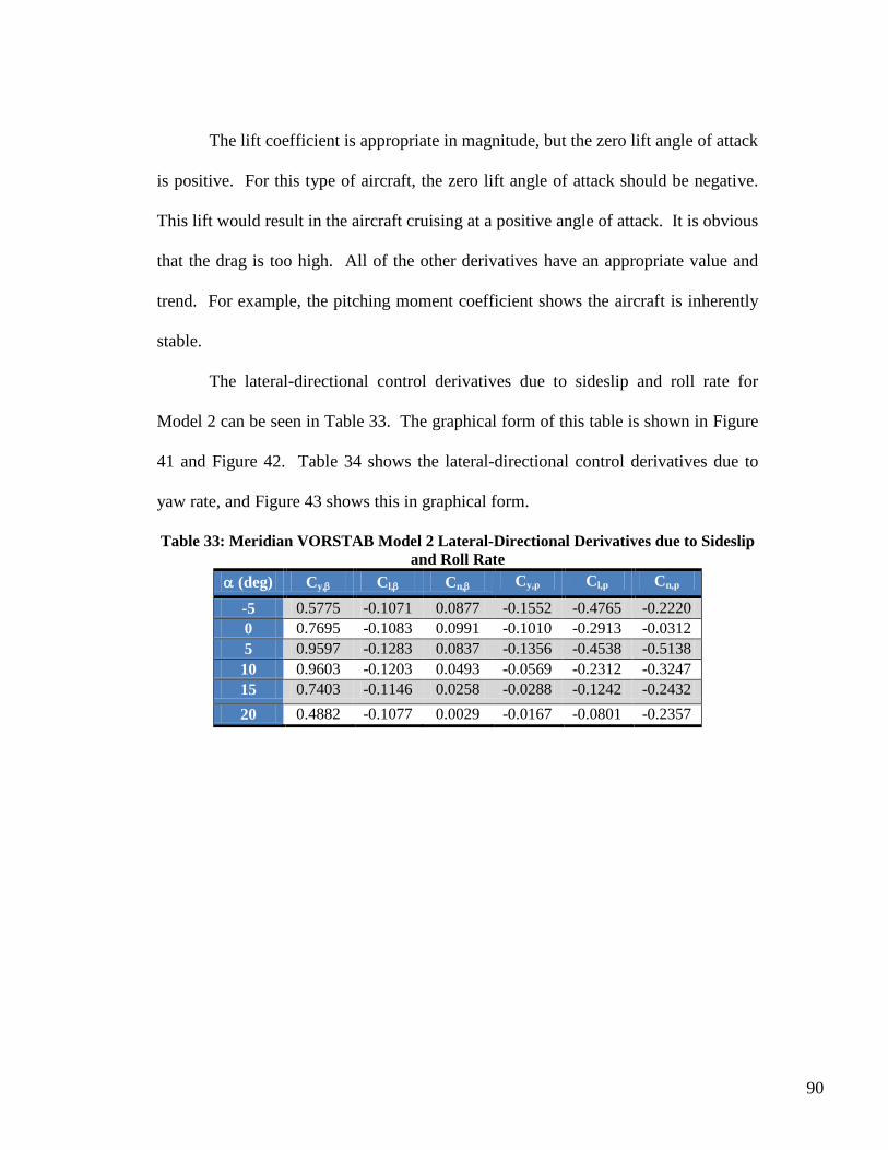
90

The lift coefficient is appropriate in magnitude, but the zero lift angle of attack

is positive. For this type of aircraft, the zero lift angle of attack should be negative.

This lift would result in the aircraft cruising at a positive angle of attack. It is obvious

that the drag is too high. All of the other derivatives have an appropriate value and

trend. For example, the pitching moment coefficient shows the aircraft is inherently

stable.

The lateral-directional control derivatives due to sideslip and roll rate for

Model 2 can be seen in Table 33. The graphical form of this table is shown in Figure

41 and Figure 42. Table 34 shows the lateral-directional control derivatives due to

yaw rate, and Figure 43 shows this in graphical form.

Table 33: Meridian VORSTAB Model 2 Lateral-Directional Derivatives due to Sideslip

and Roll Rate

(deg) Cy, Cl, Cn, Cy,p Cl,p Cn,p

-5 0.5775 -0.1071 0.0877 -0.1552 -0.4765 -0.2220

0 0.7695 -0.1083 0.0991 -0.1010 -0.2913 -0.0312

5 0.9597 -0.1283 0.0837 -0.1356 -0.4538 -0.5138

10 0.9603 -0.1203 0.0493 -0.0569 -0.2312 -0.3247

15 0.7403 -0.1146 0.0258 -0.0288 -0.1242 -0.2432

20 0.4882 -0.1077 0.0029 -0.0167 -0.0801 -0.2357

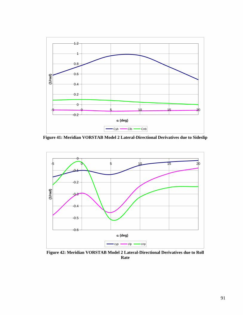
91

-0.2

0

0.2

0.4

0.6

0.8

1

1.2

-5 0 5 10 15 20

(1/r

ad

)

(deg)

Cyb Clb Cnb

Figure 41: Meridian VORSTAB Model 2 Lateral-Directional Derivatives due to Sideslip

-0.6

-0.5

-0.4

-0.3

-0.2

-0.1

0

-5 0 5 10 15 20

(1/r

ad

)

(deg)

cyp clp cnp


Rate

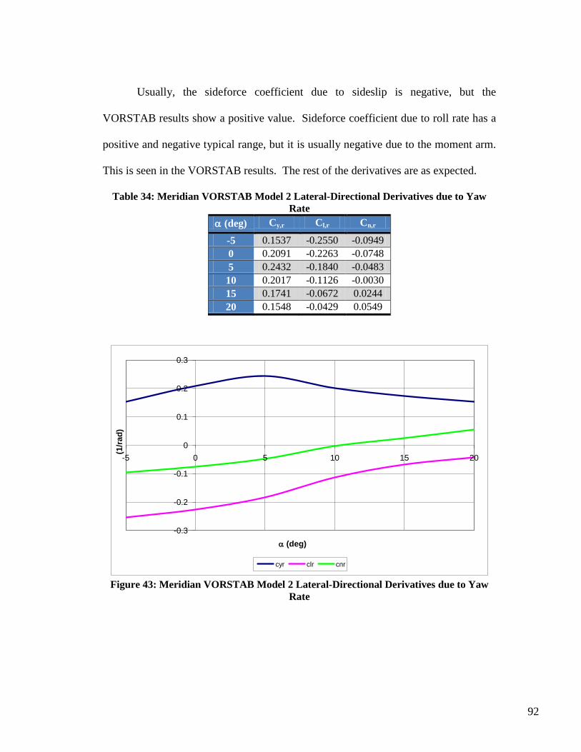
92

Usually, the sideforce coefficient due to sideslip is negative, but the

VORSTAB results show a positive value. Sideforce coefficient due to roll rate has a

positive and negative typical range, but it is usually negative due to the moment arm.

This is seen in the VORSTAB results. The rest of the derivatives are as expected.

Table 34: Meridian VORSTAB Model 2 Lateral-Directional Derivatives due to Yaw

Rate

(deg) Cy,r Cl,r Cn,r

-5 0.1537 -0.2550 -0.0949

0 0.2091 -0.2263 -0.0748

5 0.2432 -0.1840 -0.0483

10 0.2017 -0.1126 -0.0030

15 0.1741 -0.0672 0.0244

20 0.1548 -0.0429 0.0549

-0.3

-0.2

-0.1

0

0.1

0.2

0.3

-5 0 5 10 15 20

(1/r

ad

)

(deg)

cyr clr cnr

Figure 43: Meridian VORSTAB Model 2 Lateral-Directional Derivatives due to Yaw

Rate

93

The lateral-directional derivatives due to yaw rate have values that are

expected, except for the rolling moment coefficient. This derivative is normally a

positive value, since the wing-fuselage contribution is always positive and outweighs

the vertical tail contribution. The vertical tail contribution can be either positive or

negative. This vertical tail contribution outweighs the wing-fuselage contribution for

this aircraft since it has a negative value.

Deflecting the control surfaces affects the stability and control derivatives.

Table 35 through Table 37 show the control derivatives due to different control

surface deflections. These three tables are also graphical depicted in Figure 44

through Figure 52. The Meridian has a v-tail so there is not a conventional rudder or

elevators. The v-tail imitates a rudder input with an asymmetrical deflection of the

tails and imitates an elevator input with a symmetrical deflection of the tails. These

types of control surfaces are called rudevators.

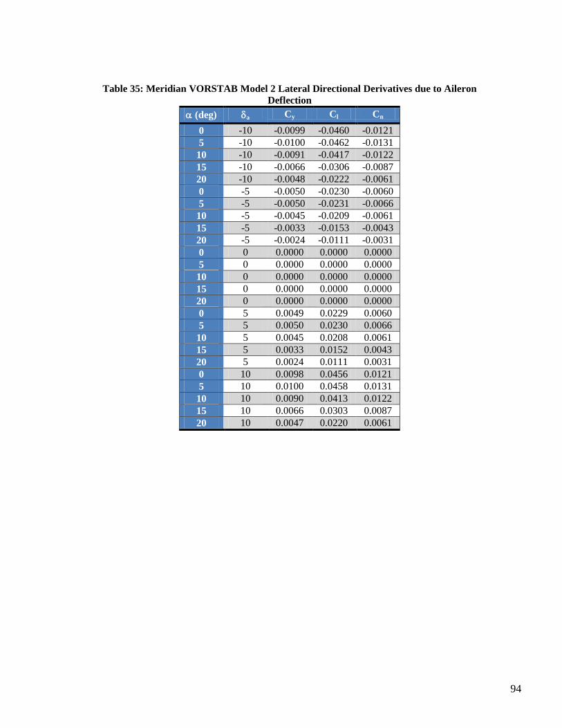
94

Table 35: Meridian VORSTAB Model 2 Lateral Directional Derivatives due to Aileron

Deflection

(deg) a Cy Cl Cn

0 -10 -0.0099 -0.0460 -0.0121

5 -10 -0.0100 -0.0462 -0.0131

10 -10 -0.0091 -0.0417 -0.0122

15 -10 -0.0066 -0.0306 -0.0087

20 -10 -0.0048 -0.0222 -0.0061

0 -5 -0.0050 -0.0230 -0.0060

5 -5 -0.0050 -0.0231 -0.0066

10 -5 -0.0045 -0.0209 -0.0061

15 -5 -0.0033 -0.0153 -0.0043

20 -5 -0.0024 -0.0111 -0.0031

0 0 0.0000 0.0000 0.0000

5 0 0.0000 0.0000 0.0000

10 0 0.0000 0.0000 0.0000

15 0 0.0000 0.0000 0.0000

20 0 0.0000 0.0000 0.0000

0 5 0.0049 0.0229 0.0060

5 5 0.0050 0.0230 0.0066

10 5 0.0045 0.0208 0.0061

15 5 0.0033 0.0152 0.0043

20 5 0.0024 0.0111 0.0031

0 10 0.0098 0.0456 0.0121

5 10 0.0100 0.0458 0.0131

10 10 0.0090 0.0413 0.0122

15 10 0.0066 0.0303 0.0087

20 10 0.0047 0.0220 0.0061

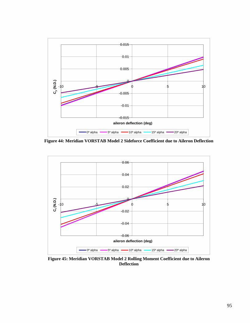
95

-0.015

-0.01

-0.005

0

0.005

0.01

0.015

-10 -5 0 5 10

Cy

(N.D

.)



Figure 44: Meridian VORSTAB Model 2 Sideforce Coefficient due to Aileron Deflection

-0.06

-0.04

-0.02

0

0.02

0.04

0.06

-10 -5 0 5 10

Cl(N

.D.)




Deflection

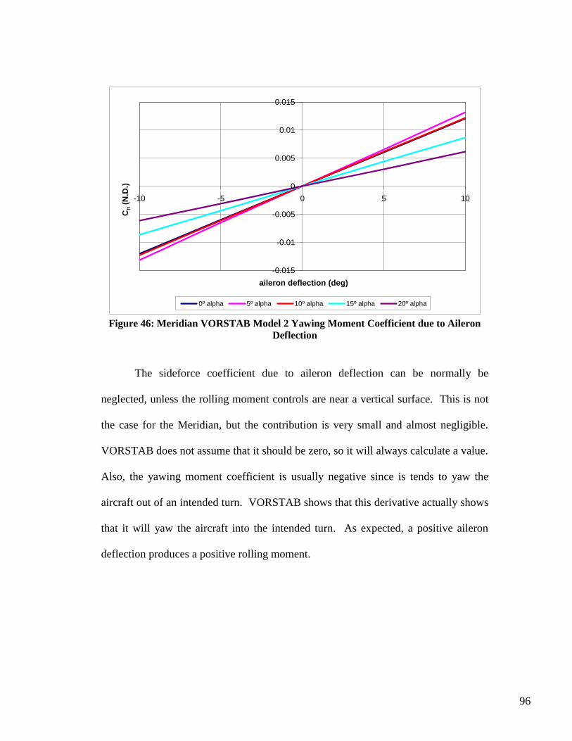
96

-0.015

-0.01

-0.005

0

0.005

0.01

0.015

-10 -5 0 5 10

Cn

(N.D

.)




Deflection

The sideforce coefficient due to aileron deflection can be normally be

neglected, unless the rolling moment controls are near a vertical surface. This is not

the case for the Meridian, but the contribution is very small and almost negligible.

VORSTAB does not assume that it should be zero, so it will always calculate a value.

Also, the yawing moment coefficient is usually negative since is tends to yaw the

aircraft out of an intended turn. VORSTAB shows that this derivative actually shows

that it will yaw the aircraft into the intended turn. As expected, a positive aileron

deflection produces a positive rolling moment.

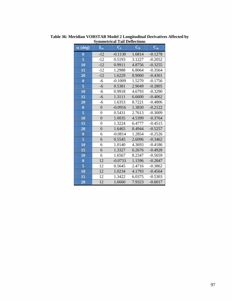
97

Table 36: Meridian VORSTAB Model 2 Longitudinal Derivatives Affected by

Symmetrical Tail Deflections

(deg) re CL CD Cm

0 -12 -0.1130 1.6814 -0.1278

5 -12 0.5193 3.1227 -0.2052

10 -12 0.9911 4.8756 -0.3255

15 -12 1.2988 6.8064 -0.3564

20 -12 1.6229 8.9060 -0.4301

0 -6 -0.1009 1.5270 -0.1756

5 -6 0.5381 2.9049 -0.2805

10 -6 0.9918 4.6793 -0.3290

15 -6 1.3111 6.6600 -0.4062

20 -6 1.6353 8.7221 -0.4806

0 0 -0.0916 1.3830 -0.2122

5 0 0.5431 2.7613 -0.3009

10 0 1.0035 4.5399 -0.3764

15 0 1.3224 6.4777 -0.4515

20 0 1.6465 8.4944 -0.5257

0 6 -0.0814 1.2854 -0.2526

5 6 0.5545 2.6096 -0.3462

10 6 1.0140 4.3693 -0.4186

15 6 1.3327 6.2676 -0.4928

20 6 1.6567 8.2347 -0.5659

0 12 -0.0733 1.1596 -0.2847

5 12 0.5645 2.4716 -0.3862

10 12 1.0234 4.1793 -0.4564

15 12 1.3422 6.0375 -0.5303

20 12 1.6660 7.9323 -0.6017

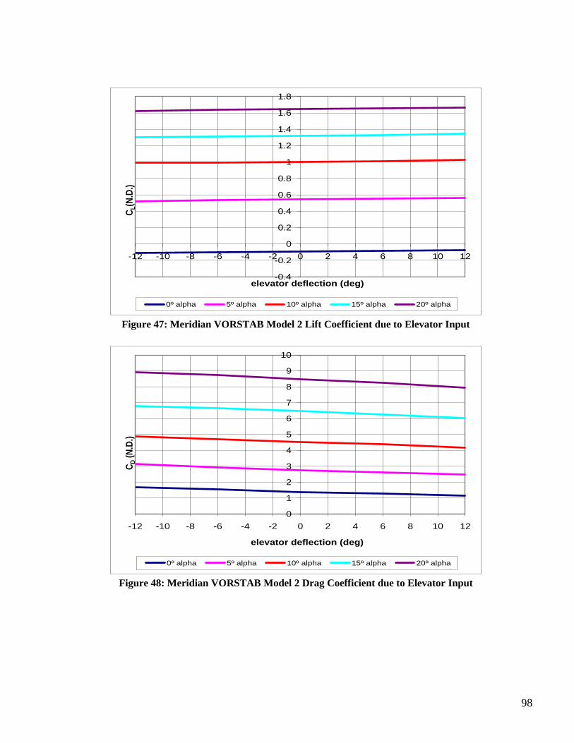
98

-0.4

-0.2

0

0.2

0.4

0.6

0.8

1

1.2

1.4

1.6

1.8

-12 -10 -8 -6 -4 -2 0 2 4 6 8 10 12

CL(N

.D.)



Figure 47: Meridian VORSTAB Model 2 Lift Coefficient due to Elevator Input

0

1

2

3

4

5

6

7

8

9

10

-12 -10 -8 -6 -4 -2 0 2 4 6 8 10 12

CD

(N.D

.)



Figure 48: Meridian VORSTAB Model 2 Drag Coefficient due to Elevator Input

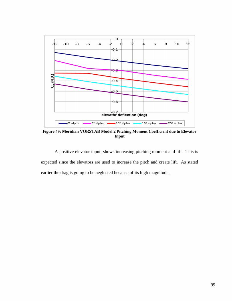
99

-0.7

-0.6

-0.5

-0.4

-0.3

-0.2

-0.1

0

-12 -10 -8 -6 -4 -2 0 2 4 6 8 10 12

Cm

(N.D

.)



Figure 49: Meridian VORSTAB Model 2 Pitching Moment Coefficient due to Elevator

Input

A positive elevator input, shows increasing pitching moment and lift. This is

expected since the elevators are used to increase the pitch and create lift. As stated

earlier the drag is going to be neglected because of its high magnitude.

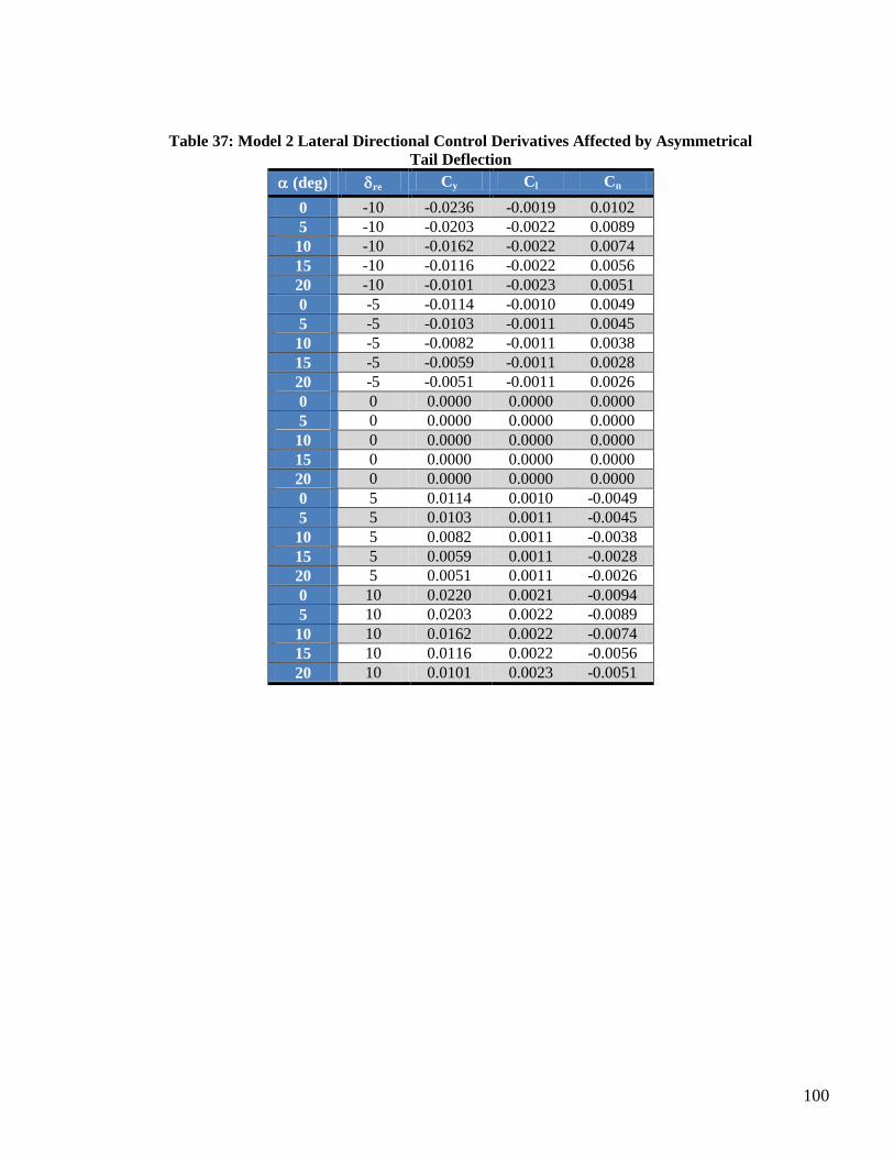
100

Table 37: Model 2 Lateral Directional Control Derivatives Affected by Asymmetrical

Tail Deflection

(deg) re Cy Cl Cn

0 -10 -0.0236 -0.0019 0.0102

5 -10 -0.0203 -0.0022 0.0089

10 -10 -0.0162 -0.0022 0.0074

15 -10 -0.0116 -0.0022 0.0056

20 -10 -0.0101 -0.0023 0.0051

0 -5 -0.0114 -0.0010 0.0049

5 -5 -0.0103 -0.0011 0.0045

10 -5 -0.0082 -0.0011 0.0038

15 -5 -0.0059 -0.0011 0.0028

20 -5 -0.0051 -0.0011 0.0026

0 0 0.0000 0.0000 0.0000

5 0 0.0000 0.0000 0.0000

10 0 0.0000 0.0000 0.0000

15 0 0.0000 0.0000 0.0000

20 0 0.0000 0.0000 0.0000

0 5 0.0114 0.0010 -0.0049

5 5 0.0103 0.0011 -0.0045

10 5 0.0082 0.0011 -0.0038

15 5 0.0059 0.0011 -0.0028

20 5 0.0051 0.0011 -0.0026

0 10 0.0220 0.0021 -0.0094

5 10 0.0203 0.0022 -0.0089

10 10 0.0162 0.0022 -0.0074

15 10 0.0116 0.0022 -0.0056

20 10 0.0101 0.0023 -0.0051

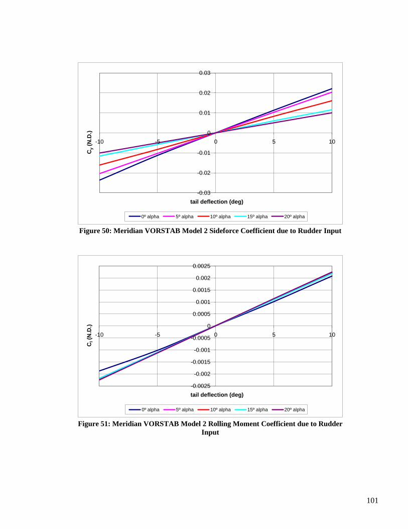
101

-0.03

-0.02

-0.01

0

0.01

0.02

0.03

-10 -5 0 5 10

Cy

(N.D

.)

tail deflection (deg)


Figure 50: Meridian VORSTAB Model 2 Sideforce Coefficient due to Rudder Input

-0.0025

-0.002

-0.0015

-0.001

-0.0005

0

0.0005

0.001

0.0015

0.002

0.0025

-10 -5 0 5 10

Cl(N

.D.)



Figure 51: Meridian VORSTAB Model 2 Rolling Moment Coefficient due to Rudder

Input

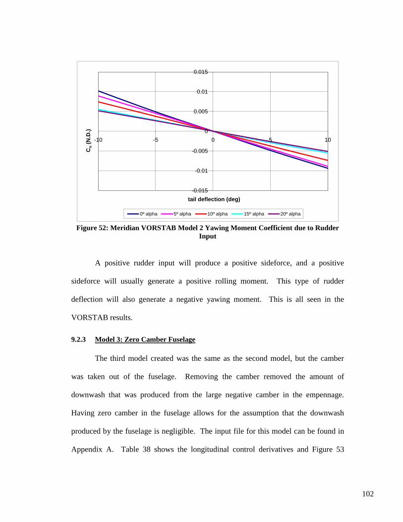
102

-0.015

-0.01

-0.005

0

0.005

0.01

0.015

-10 -5 0 5 10

Cn

(N.D

.)



Figure 52: Meridian VORSTAB Model 2 Yawing Moment Coefficient due to Rudder

Input

A positive rudder input will produce a positive sideforce, and a positive

sideforce will usually generate a positive rolling moment. This type of rudder

deflection will also generate a negative yawing moment. This is all seen in the

VORSTAB results.

9.2.3 Model 3: Zero Camber Fuselage

The third model created was the same as the second model, but the camber

was taken out of the fuselage. Removing the camber removed the amount of

downwash that was produced from the large negative camber in the empennage.

Having zero camber in the fuselage allows for the assumption that the downwash

produced by the fuselage is negligible. The input file for this model can be found in

Appendix A. Table 38 shows the longitudinal control derivatives and Figure 53

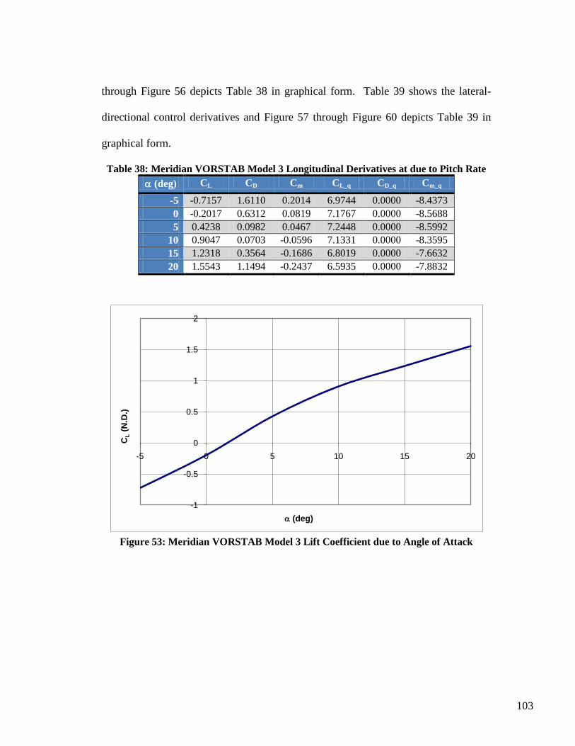
103

through Figure 56 depicts Table 38 in graphical form. Table 39 shows the lateral-

directional control derivatives and Figure 57 through Figure 60 depicts Table 39 in

graphical form.

Table 38: Meridian VORSTAB Model 3 Longitudinal Derivatives at due to Pitch Rate

(deg) CL CD Cm CL_q CD_q Cm_q

-5 -0.7157 1.6110 0.2014 6.9744 0.0000 -8.4373

0 -0.2017 0.6312 0.0819 7.1767 0.0000 -8.5688

5 0.4238 0.0982 0.0467 7.2448 0.0000 -8.5992

10 0.9047 0.0703 -0.0596 7.1331 0.0000 -8.3595

15 1.2318 0.3564 -0.1686 6.8019 0.0000 -7.6632

20 1.5543 1.1494 -0.2437 6.5935 0.0000 -7.8832

-1

-0.5

0

0.5

1

1.5

2

-5 0 5 10 15 20

CL

(N.D

.)

(deg)


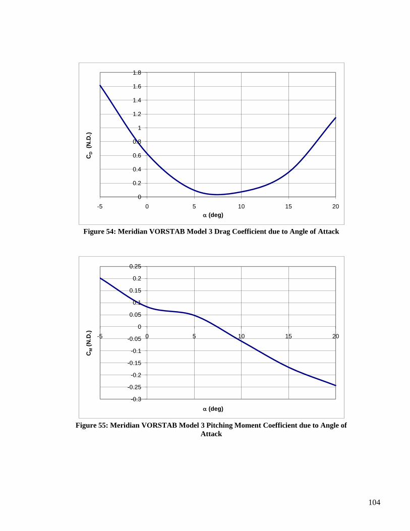
104

0

0.2

0.4

0.6

0.8

1

1.2

1.4

1.6

1.8

-5 0 5 10 15 20

CD

(N.D

.)

(deg)


-0.3

-0.25

-0.2

-0.15

-0.1

-0.05

0

0.05

0.1

0.15

0.2

0.25

-5 0 5 10 15 20

CM

(N.D

.)

(deg)


Attack

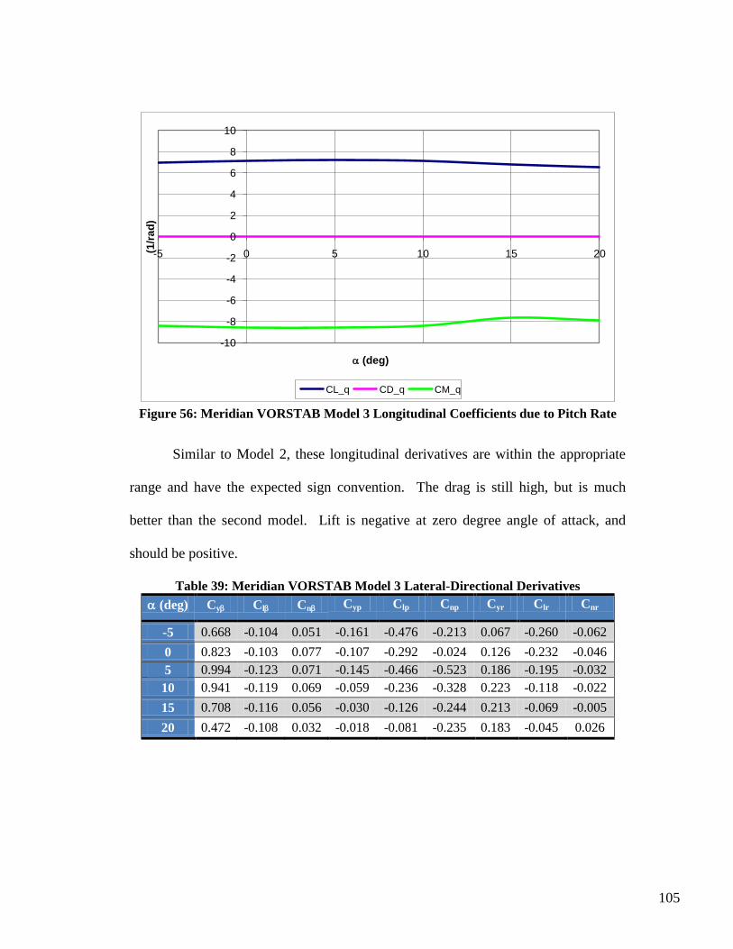
105

-10

-8

-6

-4

-2

0

2

4

6

8

10

-5 0 5 10 15 20(1/r

ad

)

(deg)

CL_q CD_q CM_q

Figure 56: Meridian VORSTAB Model 3 Longitudinal Coefficients due to Pitch Rate

Similar to Model 2, these longitudinal derivatives are within the appropriate

range and have the expected sign convention. The drag is still high, but is much

better than the second model. Lift is negative at zero degree angle of attack, and

should be positive.

Table 39: Meridian VORSTAB Model 3 Lateral-Directional Derivatives


-5 0.668 -0.104 0.051 -0.161 -0.476 -0.213 0.067 -0.260 -0.062

0 0.823 -0.103 0.077 -0.107 -0.292 -0.024 0.126 -0.232 -0.046

5 0.994 -0.123 0.071 -0.145 -0.466 -0.523 0.186 -0.195 -0.032

10 0.941 -0.119 0.069 -0.059 -0.236 -0.328 0.223 -0.118 -0.022

15 0.708 -0.116 0.056 -0.030 -0.126 -0.244 0.213 -0.069 -0.005

20 0.472 -0.108 0.032 -0.018 -0.081 -0.235 0.183 -0.045 0.026

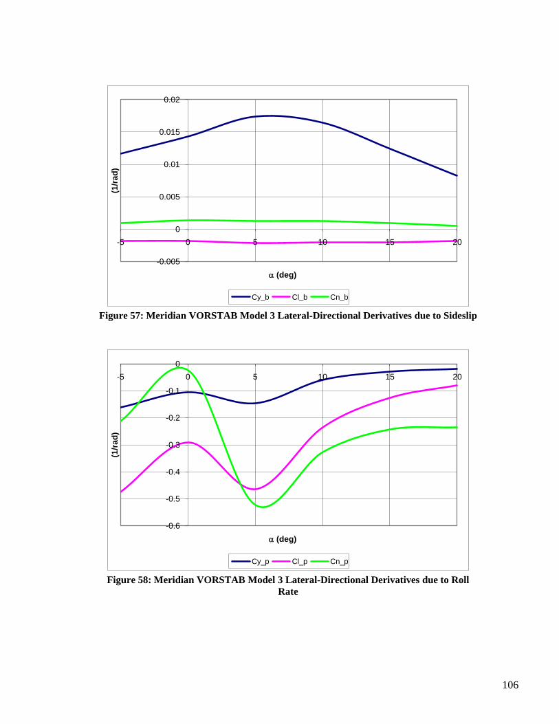
106

-0.005

0

0.005

0.01

0.015

0.02

-5 0 5 10 15 20

(1/r

ad

)

(deg)

Cy_b Cl_b Cn_b


-0.6

-0.5

-0.4

-0.3

-0.2

-0.1

0

-5 0 5 10 15 20

(1/r

ad

)

(deg)

Cy_p Cl_p Cn_p


Rate

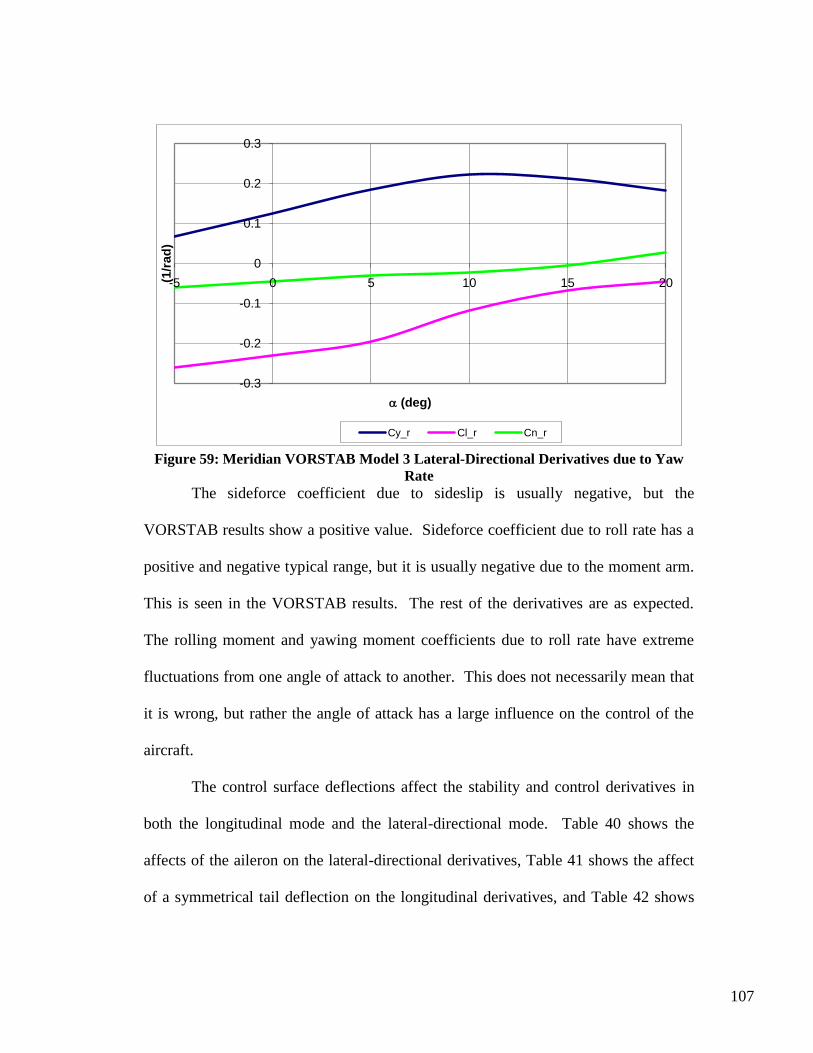
107

-0.3

-0.2

-0.1

0

0.1

0.2

0.3

-5 0 5 10 15 20(1/r

ad

)

(deg)

Cy_r Cl_r Cn_r

Figure 59: Meridian VORSTAB Model 3 Lateral-Directional Derivatives due to Yaw

Rate

The sideforce coefficient due to sideslip is usually negative, but the

VORSTAB results show a positive value. Sideforce coefficient due to roll rate has a

positive and negative typical range, but it is usually negative due to the moment arm.

This is seen in the VORSTAB results. The rest of the derivatives are as expected.

The rolling moment and yawing moment coefficients due to roll rate have extreme

fluctuations from one angle of attack to another. This does not necessarily mean that

it is wrong, but rather the angle of attack has a large influence on the control of the

aircraft.

The control surface deflections affect the stability and control derivatives in

both the longitudinal mode and the lateral-directional mode. Table 40 shows the

affects of the aileron on the lateral-directional derivatives, Table 41 shows the affect

of a symmetrical tail deflection on the longitudinal derivatives, and Table 42 shows

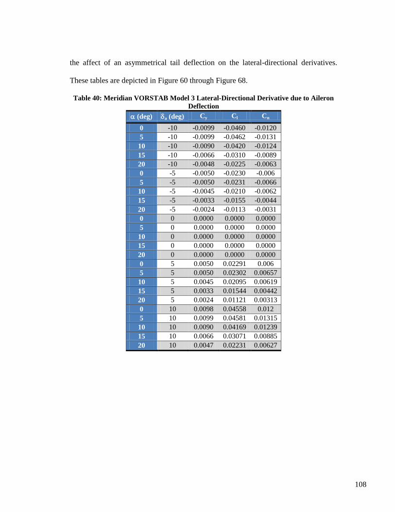
108

the affect of an asymmetrical tail deflection on the lateral-directional derivatives.

These tables are depicted in Figure 60 through Figure 68.

Table 40: Meridian VORSTAB Model 3 Lateral-Directional Derivative due to Aileron

Deflection

(deg) a (deg) Cy Cl Cn

0 -10 -0.0099 -0.0460 -0.0120

5 -10 -0.0099 -0.0462 -0.0131

10 -10 -0.0090 -0.0420 -0.0124

15 -10 -0.0066 -0.0310 -0.0089

20 -10 -0.0048 -0.0225 -0.0063

0 -5 -0.0050 -0.0230 -0.006

5 -5 -0.0050 -0.0231 -0.0066

10 -5 -0.0045 -0.0210 -0.0062

15 -5 -0.0033 -0.0155 -0.0044

20 -5 -0.0024 -0.0113 -0.0031

0 0 0.0000 0.0000 0.0000

5 0 0.0000 0.0000 0.0000

10 0 0.0000 0.0000 0.0000

15 0 0.0000 0.0000 0.0000

20 0 0.0000 0.0000 0.0000

0 5 0.0050 0.02291 0.006

5 5 0.0050 0.02302 0.00657

10 5 0.0045 0.02095 0.00619

15 5 0.0033 0.01544 0.00442

20 5 0.0024 0.01121 0.00313

0 10 0.0098 0.04558 0.012

5 10 0.0099 0.04581 0.01315

10 10 0.0090 0.04169 0.01239

15 10 0.0066 0.03071 0.00885

20 10 0.0047 0.02231 0.00627

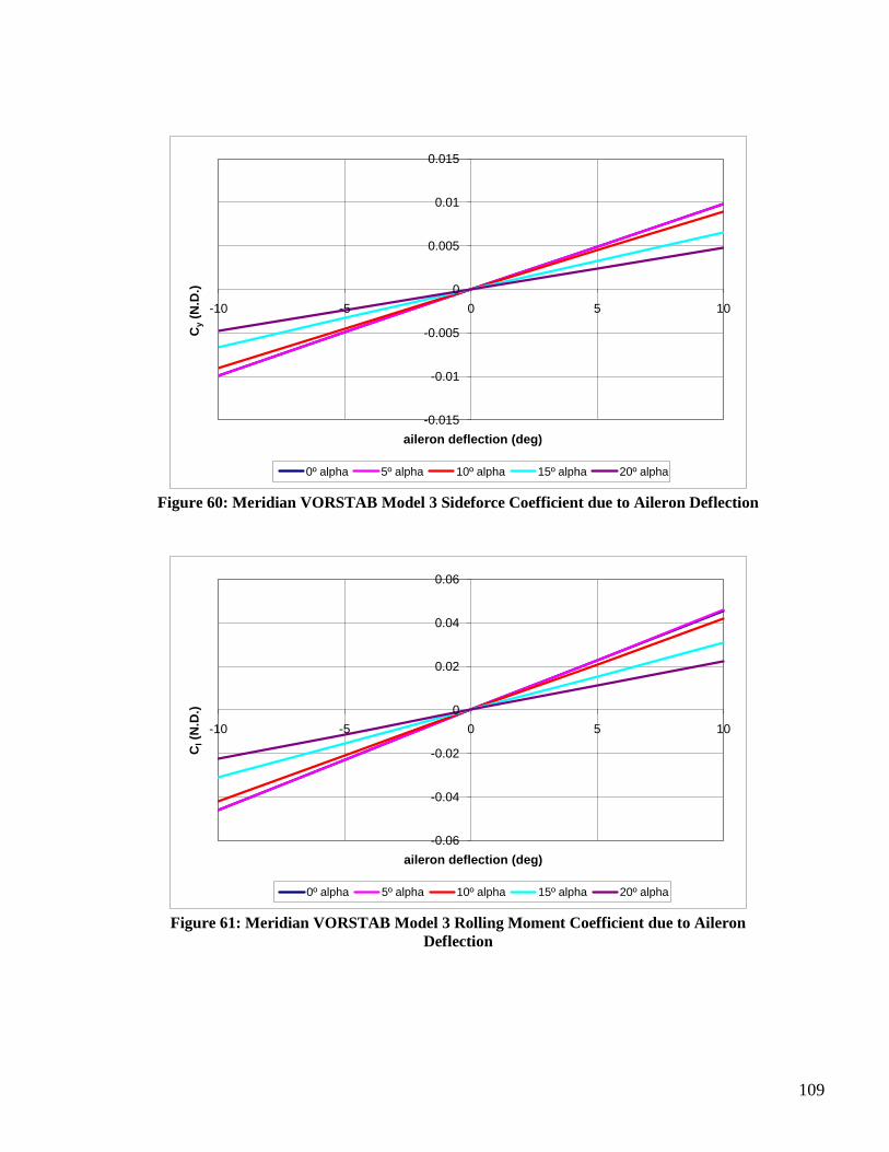
109

-0.015

-0.01

-0.005

0

0.005

0.01

0.015

-10 -5 0 5 10

Cy

(N.D

.)




-0.06

-0.04

-0.02

0

0.02

0.04

0.06

-10 -5 0 5 10

Cl(N

.D.)




Deflection

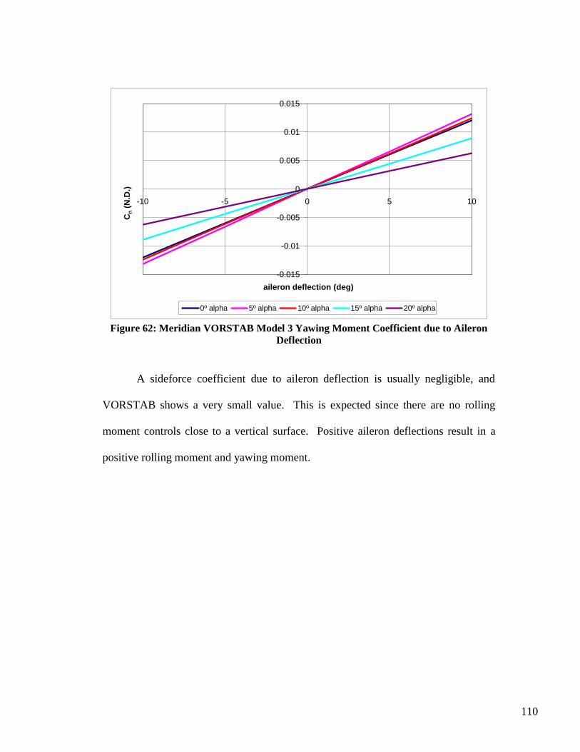
110

-0.015

-0.01

-0.005

0

0.005

0.01

0.015

-10 -5 0 5 10

Cn

(N.D

.)




Deflection

A sideforce coefficient due to aileron deflection is usually negligible, and

VORSTAB shows a very small value. This is expected since there are no rolling

moment controls close to a vertical surface. Positive aileron deflections result in a

positive rolling moment and yawing moment.

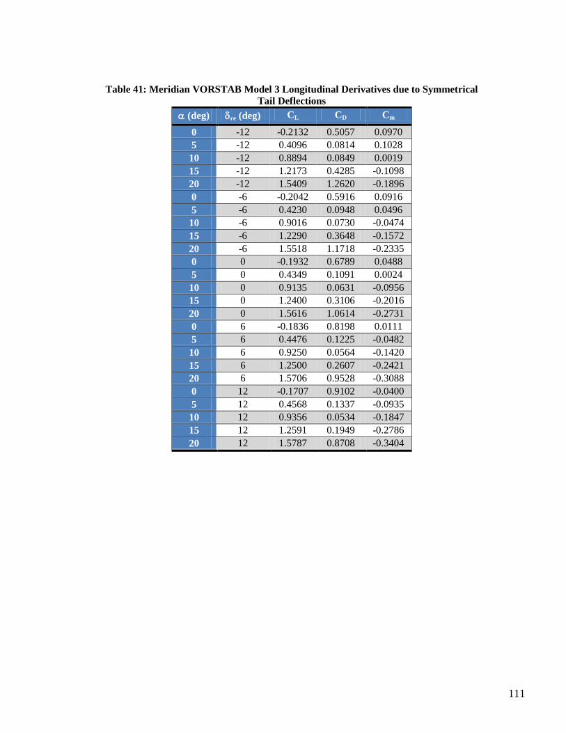
111

Table 41: Meridian VORSTAB Model 3 Longitudinal Derivatives due to Symmetrical

Tail Deflections

(deg) re (deg) CL CD Cm

0 -12 -0.2132 0.5057 0.0970

5 -12 0.4096 0.0814 0.1028

10 -12 0.8894 0.0849 0.0019

15 -12 1.2173 0.4285 -0.1098

20 -12 1.5409 1.2620 -0.1896

0 -6 -0.2042 0.5916 0.0916

5 -6 0.4230 0.0948 0.0496

10 -6 0.9016 0.0730 -0.0474

15 -6 1.2290 0.3648 -0.1572

20 -6 1.5518 1.1718 -0.2335

0 0 -0.1932 0.6789 0.0488

5 0 0.4349 0.1091 0.0024

10 0 0.9135 0.0631 -0.0956

15 0 1.2400 0.3106 -0.2016

20 0 1.5616 1.0614 -0.2731

0 6 -0.1836 0.8198 0.0111

5 6 0.4476 0.1225 -0.0482

10 6 0.9250 0.0564 -0.1420

15 6 1.2500 0.2607 -0.2421

20 6 1.5706 0.9528 -0.3088

0 12 -0.1707 0.9102 -0.0400

5 12 0.4568 0.1337 -0.0935

10 12 0.9356 0.0534 -0.1847

15 12 1.2591 0.1949 -0.2786

20 12 1.5787 0.8708 -0.3404

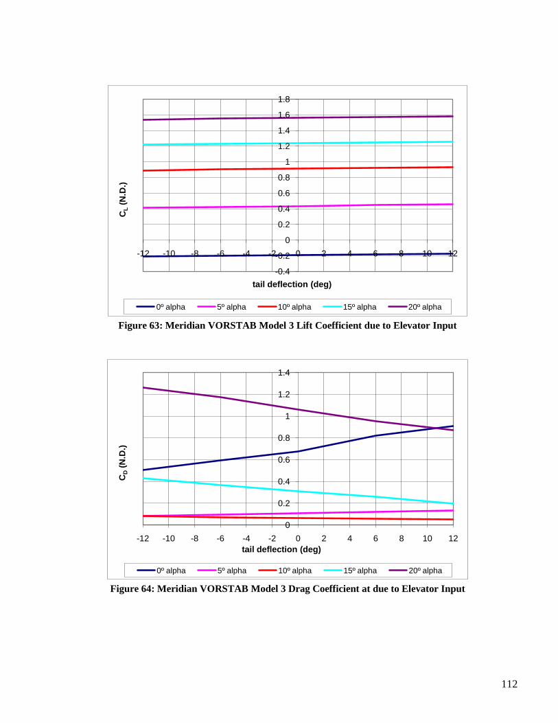
112

-0.4

-0.2

0

0.2

0.4

0.6

0.8

1

1.2

1.4

1.6

1.8

-12 -10 -8 -6 -4 -2 0 2 4 6 8 10 12

CL

(N.D

.)




0

0.2

0.4

0.6

0.8

1

1.2

1.4

-12 -10 -8 -6 -4 -2 0 2 4 6 8 10 12

CD

(N.D

.)



Figure 64: Meridian VORSTAB Model 3 Drag Coefficient at due to Elevator Input

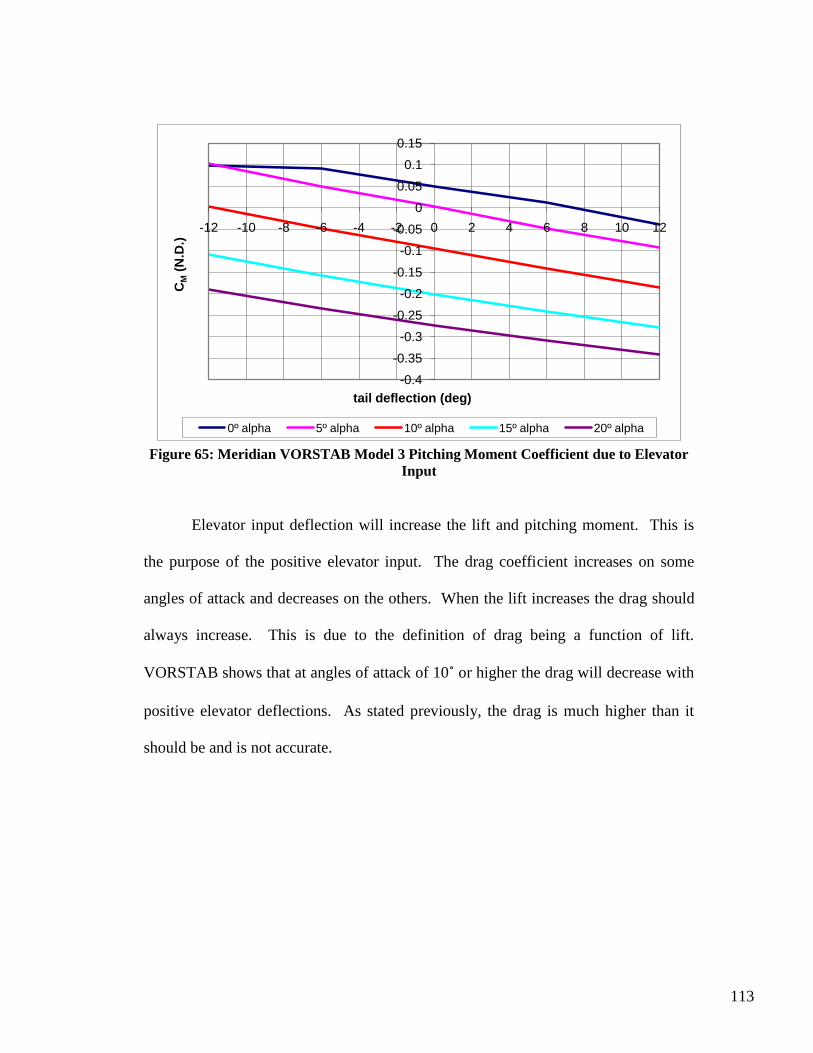
113

-0.4

-0.35

-0.3

-0.25

-0.2

-0.15

-0.1

-0.05

0

0.05

0.1

0.15

-12 -10 -8 -6 -4 -2 0 2 4 6 8 10 12

CM

(N.D

.)




Input

Elevator input deflection will increase the lift and pitching moment. This is

the purpose of the positive elevator input. The drag coefficient increases on some

angles of attack and decreases on the others. When the lift increases the drag should

always increase. This is due to the definition of drag being a function of lift.

VORSTAB shows that at angles of attack of 10˚ or higher the drag will decrease with

positive elevator deflections. As stated previously, the drag is much higher than it

should be and is not accurate.

114

Table 42: Meridian Model 3 Lateral-Directional Derivatives Affected by Asymmetrical

Tail Deflections

(deg) re (deg) Cy Cl Cn

0 -10 -0.0215 -0.0021 0.0083

5 -10 -0.0226 -0.0020 0.0092

10 -10 -0.0229 -0.0018 0.0098

15 -10 -0.0162 -0.0020 0.0070

20 -10 -0.0145 -0.0022 0.0064

0 -5 -0.0109 -0.0011 0.0042

5 -5 -0.0117 -0.0010 0.0048

10 -5 -0.0109 -0.0010 0.0046

15 -5 -0.0082 -0.0010 0.0035

20 -5 -0.0073 -0.0011 0.0033

0 0 0.0000 0.0000 0.0000

5 0 0.0000 0.0000 0.0000

10 0 0.0000 0.0000 0.0000

15 0 0.0000 0.0000 0.0000

20 0 0.0000 0.0000 0.0000

0 5 0.0109 0.0011 -0.0042

5 5 0.0123 0.0009 -0.0051

10 5 0.0109 0.0010 -0.0046

15 5 0.0082 0.0010 -0.0035

20 5 0.0073 0.0011 -0.0033

0 10 0.0215 0.0021 -0.0083

5 10 0.0239 0.0019 -0.0098

10 10 0.0209 0.0020 -0.0088

15 10 0.0162 0.0020 -0.0070

20 10 0.0145 0.0022 -0.0064

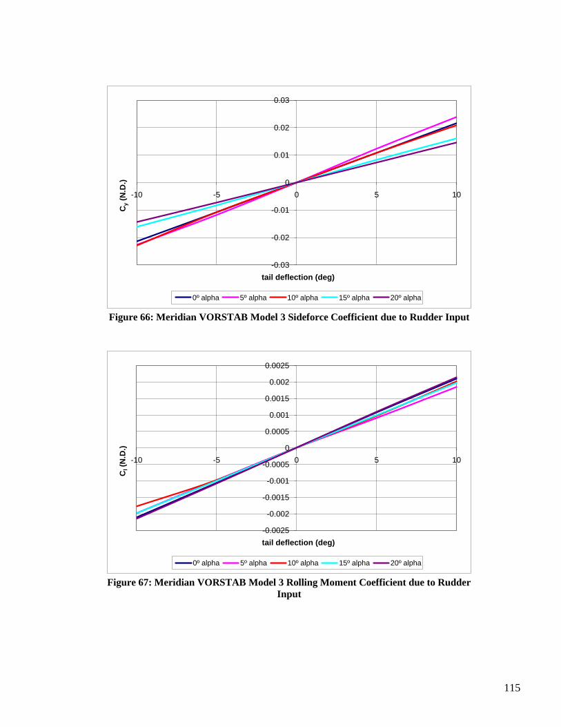
115

-0.03

-0.02

-0.01

0

0.01

0.02

0.03

-10 -5 0 5 10

Cy

(N.D

.)




-0.0025

-0.002

-0.0015

-0.001

-0.0005

0

0.0005

0.001

0.0015

0.002

0.0025

-10 -5 0 5 10

Cl(N

.D.)




Input

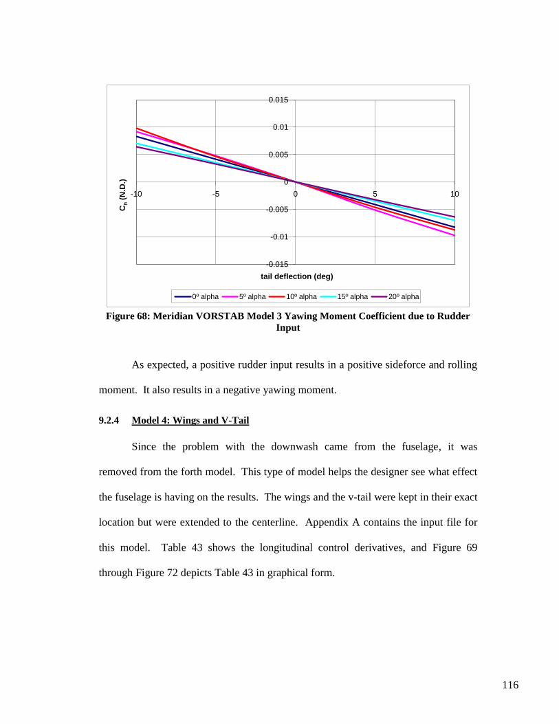
116

-0.015

-0.01

-0.005

0

0.005

0.01

0.015

-10 -5 0 5 10

Cn

(N.D

.)




Input

As expected, a positive rudder input results in a positive sideforce and rolling

moment. It also results in a negative yawing moment.

9.2.4 Model 4: Wings and V-Tail

Since the problem with the downwash came from the fuselage, it was

removed from the forth model. This type of model helps the designer see what effect

the fuselage is having on the results. The wings and the v-tail were kept in their exact

location but were extended to the centerline. Appendix A contains the input file for

this model. Table 43 shows the longitudinal control derivatives, and Figure 69

through Figure 72 depicts Table 43 in graphical form.

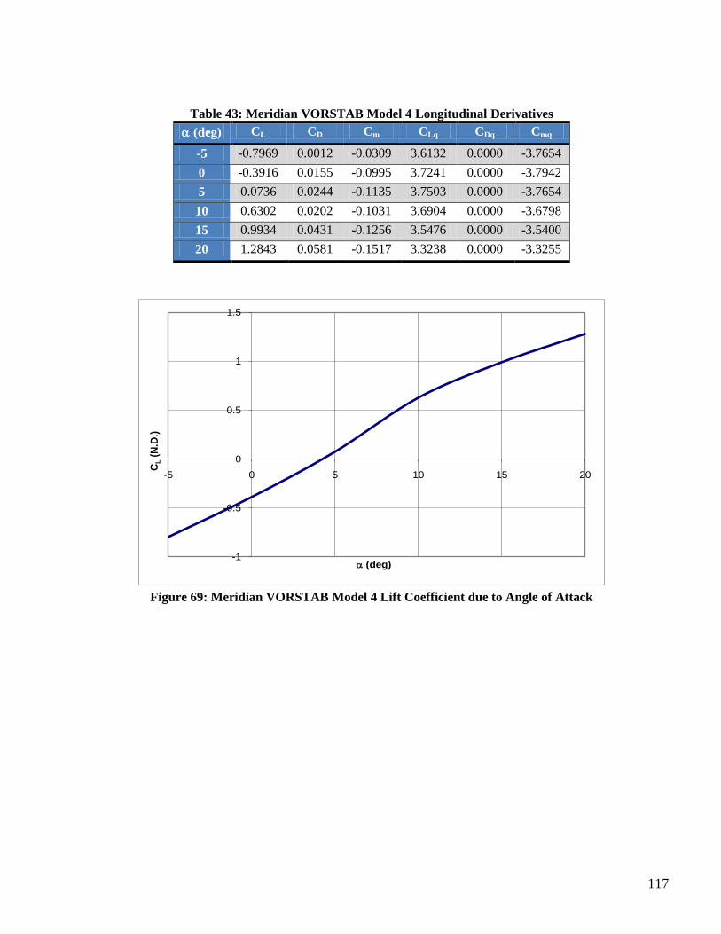
117

Table 43: Meridian VORSTAB Model 4 Longitudinal Derivatives

(deg) CL CD Cm CLq CDq Cmq

-5 -0.7969 0.0012 -0.0309 3.6132 0.0000 -3.7654

0 -0.3916 0.0155 -0.0995 3.7241 0.0000 -3.7942

5 0.0736 0.0244 -0.1135 3.7503 0.0000 -3.7654

10 0.6302 0.0202 -0.1031 3.6904 0.0000 -3.6798

15 0.9934 0.0431 -0.1256 3.5476 0.0000 -3.5400

20 1.2843 0.0581 -0.1517 3.3238 0.0000 -3.3255

-1

-0.5

0

0.5

1

1.5

-5 0 5 10 15 20

CL

(N.D

.)

(deg)


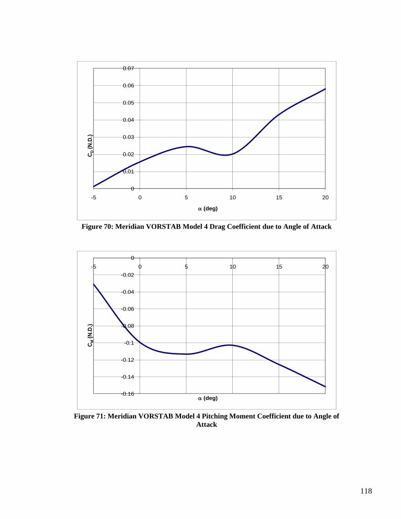
118

0

0.01

0.02

0.03

0.04

0.05

0.06

0.07

-5 0 5 10 15 20

CD

(N.D

.)

(deg)


-0.16

-0.14

-0.12

-0.1

-0.08

-0.06

-0.04

-0.02

0

-5 0 5 10 15 20

CM

(N.D

.)

(deg)


Attack

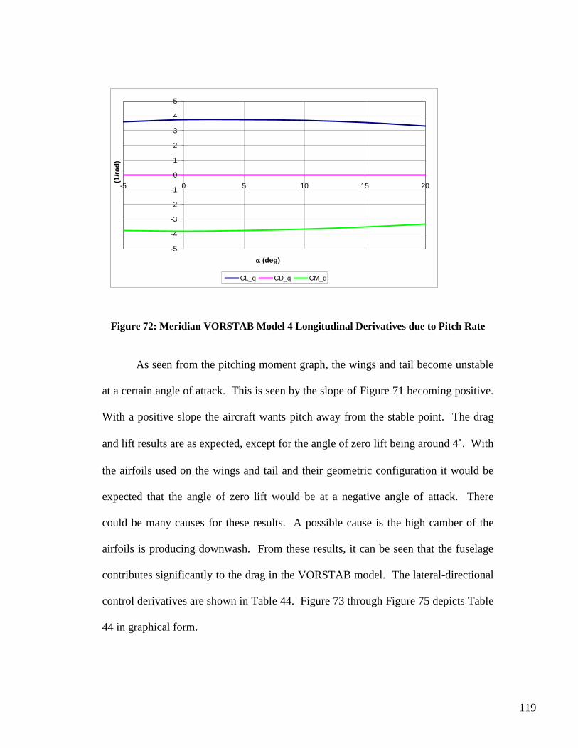
119

-5

-4

-3

-2

-1

0

1

2

3

4

5

-5 0 5 10 15 20

(1/r

ad

)

(deg)

CL_q CD_q CM_q

Figure 72: Meridian VORSTAB Model 4 Longitudinal Derivatives due to Pitch Rate

As seen from the pitching moment graph, the wings and tail become unstable

at a certain angle of attack. This is seen by the slope of Figure 71 becoming positive.

With a positive slope the aircraft wants pitch away from the stable point. The drag

and lift results are as expected, except for the angle of zero lift being around 4˚. With

the airfoils used on the wings and tail and their geometric configuration it would be

expected that the angle of zero lift would be at a negative angle of attack. There

could be many causes for these results. A possible cause is the high camber of the

airfoils is producing downwash. From these results, it can be seen that the fuselage

contributes significantly to the drag in the VORSTAB model. The lateral-directional

control derivatives are shown in Table 44. Figure 73 through Figure 75 depicts Table

44 in graphical form.

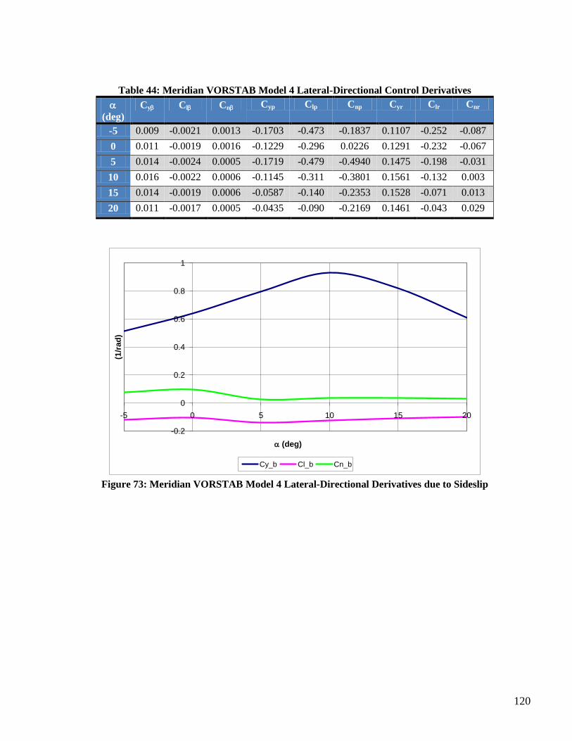
120

Table 44: Meridian VORSTAB Model 4 Lateral-Directional Control Derivatives

(deg)

Cy Cl Cn Cyp Clp Cnp Cyr Clr Cnr

-5 0.009 -0.0021 0.0013 -0.1703 -0.473 -0.1837 0.1107 -0.252 -0.087

0 0.011 -0.0019 0.0016 -0.1229 -0.296 0.0226 0.1291 -0.232 -0.067

5 0.014 -0.0024 0.0005 -0.1719 -0.479 -0.4940 0.1475 -0.198 -0.031

10 0.016 -0.0022 0.0006 -0.1145 -0.311 -0.3801 0.1561 -0.132 0.003

15 0.014 -0.0019 0.0006 -0.0587 -0.140 -0.2353 0.1528 -0.071 0.013

20 0.011 -0.0017 0.0005 -0.0435 -0.090 -0.2169 0.1461 -0.043 0.029

-0.2

0

0.2

0.4

0.6

0.8

1

-5 0 5 10 15 20

(1/r

ad

)

(deg)

Cy_b Cl_b Cn_b


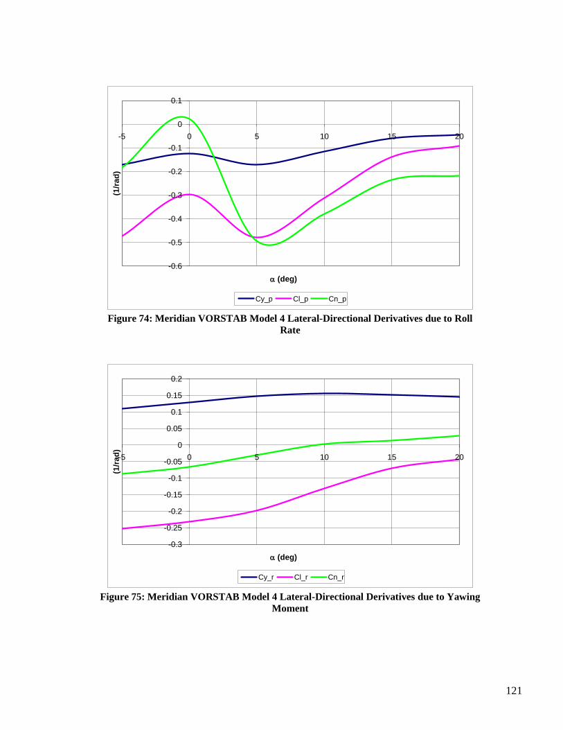
121

-0.6

-0.5

-0.4

-0.3

-0.2

-0.1

0

0.1

-5 0 5 10 15 20

(1/r

ad

)

(deg)

Cy_p Cl_p Cn_p


Rate

-0.3

-0.25

-0.2

-0.15

-0.1

-0.05

0

0.05

0.1

0.15

0.2

-5 0 5 10 15 20

(1/r

ad

)

(deg)

Cy_r Cl_r Cn_r

Figure 75: Meridian VORSTAB Model 4 Lateral-Directional Derivatives due to Yawing

Moment

122

The sideforce coefficient due to sideslip, Cy, is unstable at all angles of

attack. This can be neglected because having the fuselage will dramatically affect

this. The yawing moment coefficient due to yaw rate, Cnr, is also unstable at higher

angles of attack. A stable aircraft should naturally want to stop yawing or slow down.

When it is unstable the yawing rate increases and can lead to a spin. This will also be

influenced by the fuselage and could be stable if it were present. Table 45 shows the

lateral-directional derivatives due to an aileron deflection, Table 46 shows the

longitudinal derivatives due to a symmetrical deflection of the rudevators, and Table

47 shows the lateral-directional derivatives due to an asymmetrical deflection of the

rudevators. These tables can be seen in graphical form in Figure 76 through Figure

84.

123

Table 45: Meridian VORSTAB Model 4 Lateral-Directional Derivatives due to Aileron

Deflection

(deg) a (deg) Cy Cl Cn

0 -10 -0.0102 -0.0456 -0.0117

5 -10 -0.0103 -0.0458 -0.0127

10 -10 -0.0100 -0.0441 -0.0131

15 -10 -0.0075 -0.0336 -0.0098

20 -10 -0.0055 -0.0247 -0.0071

0 -5 -0.0051 -0.0228 -0.0059

5 -5 -0.0052 -0.0229 -0.0064

10 -5 -0.0050 -0.0221 -0.0065

15 -5 -0.0037 -0.0168 -0.0049

20 -5 -0.0027 -0.0124 -0.0035

0 0 0.0000 0.0000 0.0000

5 0 0.0000 0.0000 0.0000

10 0 0.0000 0.0000 0.0000

15 0 0.0000 0.0000 0.0000

20 0 0.0000 0.0000 0.0000

0 5 0.0051 0.0227 0.0059

5 5 0.0051 0.0228 0.0064

10 5 0.0050 0.0220 0.0065

15 5 0.0037 0.0167 0.0049

20 5 0.0027 0.0123 0.0035

0 10 0.0101 0.0452 0.0117

5 10 0.0102 0.0454 0.0127

10 10 0.0099 0.0437 0.0131

15 10 0.0074 0.0333 0.0098

20 10 0.0054 0.0245 0.0071

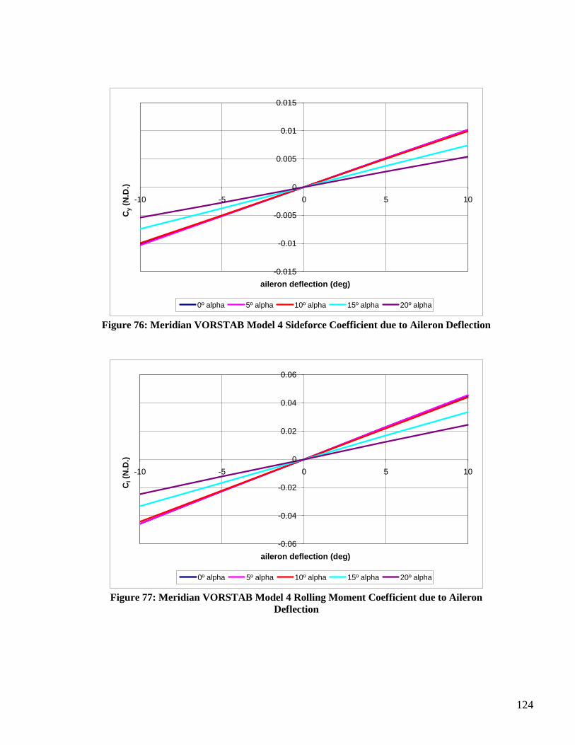
124

-0.015

-0.01

-0.005

0

0.005

0.01

0.015

-10 -5 0 5 10

Cy

(N.D

.)




-0.06

-0.04

-0.02

0

0.02

0.04

0.06

-10 -5 0 5 10

Cl(N

.D.)




Deflection

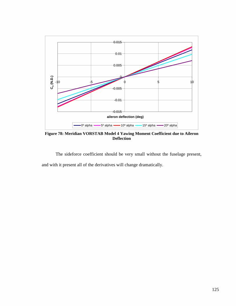
125

-0.015

-0.01

-0.005

0

0.005

0.01

0.015

-10 -5 0 5 10

Cn

(N.D

.)




Deflection

The sideforce coefficient should be very small without the fuselage present,

and with it present all of the derivatives will change dramatically.

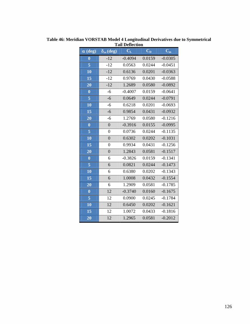
126

Table 46: Meridian VORSTAB Model 4 Longitudinal Derivatives due to Symmetrical

Tail Deflection

(deg) re (deg) CL CD Cm

0 -12 -0.4094 0.0159 -0.0305

5 -12 0.0563 0.0244 -0.0451

10 -12 0.6136 0.0201 -0.0363

15 -12 0.9769 0.0430 -0.0588

20 -12 1.2689 0.0580 -0.0892

0 -6 -0.4007 0.0159 -0.0641

5 -6 0.0649 0.0244 -0.0791

10 -6 0.6218 0.0201 -0.0693

15 -6 0.9854 0.0431 -0.0932

20 -6 1.2769 0.0580 -0.1216

0 0 -0.3916 0.0155 -0.0995

5 0 0.0736 0.0244 -0.1135

10 0 0.6302 0.0202 -0.1031

15 0 0.9934 0.0431 -0.1256

20 0 1.2843 0.0581 -0.1517

0 6 -0.3826 0.0159 -0.1341

5 6 0.0821 0.0244 -0.1473

10 6 0.6380 0.0202 -0.1343

15 6 1.0008 0.0432 -0.1554

20 6 1.2909 0.0581 -0.1785

0 12 -0.3740 0.0160 -0.1675

5 12 0.0900 0.0245 -0.1784

10 12 0.6450 0.0202 -0.1621

15 12 1.0072 0.0433 -0.1816

20 12 1.2965 0.0581 -0.2012

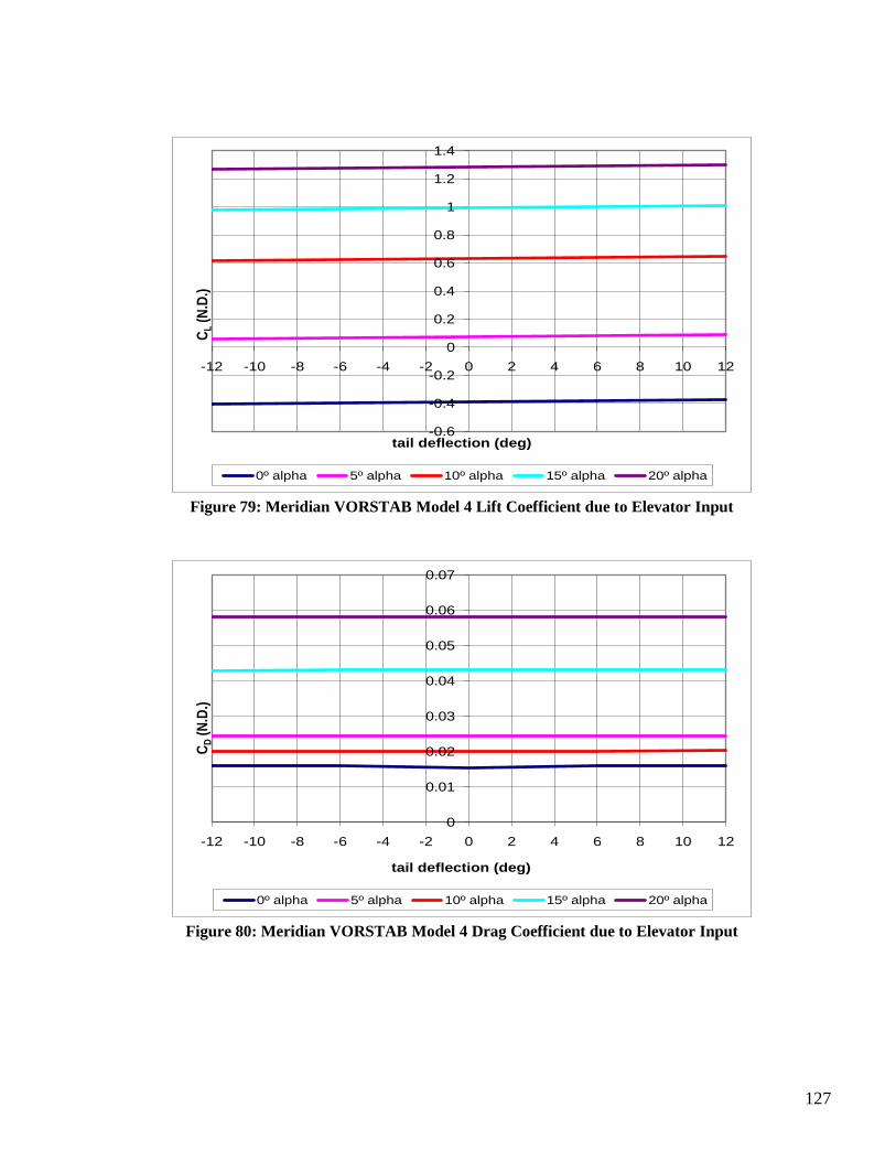
127

-0.6

-0.4

-0.2

0

0.2

0.4

0.6

0.8

1

1.2

1.4

-12 -10 -8 -6 -4 -2 0 2 4 6 8 10 12

CL

(N.D

.)




0

0.01

0.02

0.03

0.04

0.05

0.06

0.07

-12 -10 -8 -6 -4 -2 0 2 4 6 8 10 12

CD

(N.D

.)



Figure 80: Meridian VORSTAB Model 4 Drag Coefficient due to Elevator Input

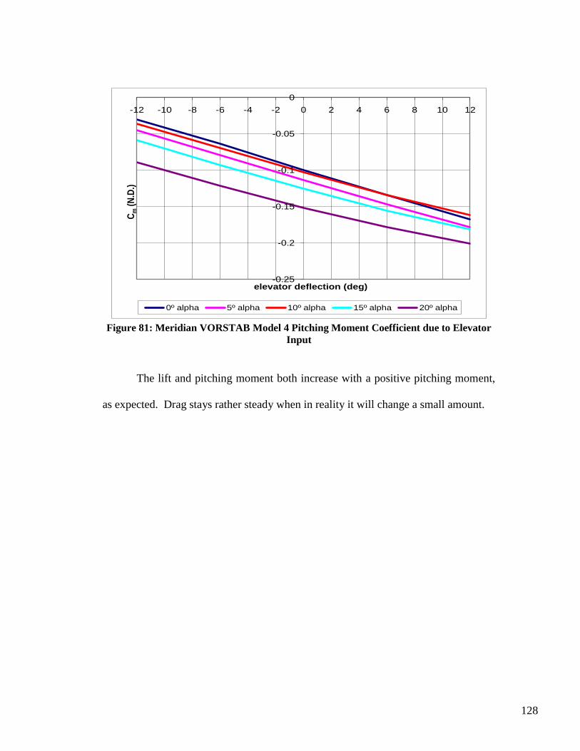
128

-0.25

-0.2

-0.15

-0.1

-0.05

0

-12 -10 -8 -6 -4 -2 0 2 4 6 8 10 12

Cm

(N.D

.)




Input

The lift and pitching moment both increase with a positive pitching moment,

as expected. Drag stays rather steady when in reality it will change a small amount.

129

Table 47: Meridian VORSTAB Model 4 Lateral-Directional Derivatives due to

Asymmetrical Deflection

(deg) re (deg) Cy Cl Cn

0 -10 -0.0246 -0.0032 0.0102

5 -10 -0.0251 -0.0031 0.0106

10 -10 -0.0252 -0.0029 0.0107

15 -10 -0.0218 -0.0032 0.0092

20 -10 -0.0198 -0.0031 0.0084

0 -5 -0.0127 -0.0016 0.0053

5 -5 -0.0129 -0.0015 0.0054

10 -5 -0.0119 -0.0016 0.0050

15 -5 -0.0110 -0.0016 0.0047

20 -5 -0.0100 -0.0016 0.0043

0 0 0.0000 0.0000 0.0000

5 0 0.0000 0.0000 0.0000

10 0 0.0000 0.0000 0.0000

15 0 0.0000 0.0000 0.0000

20 0 0.0000 0.0000 0.0000

0 5 0.0128 0.0016 -0.0053

5 5 0.0123 0.0016 -0.0052

10 5 0.0119 0.0016 -0.0050

15 5 0.0110 0.0016 -0.0047

20 5 0.0100 0.0016 -0.0043

0 10 0.0248 0.0032 -0.0103

5 10 0.0238 0.0033 -0.0100

10 10 0.0226 0.0033 -0.0095

15 10 0.0218 0.0032 -0.0092

20 10 0.0198 0.0031 -0.0084

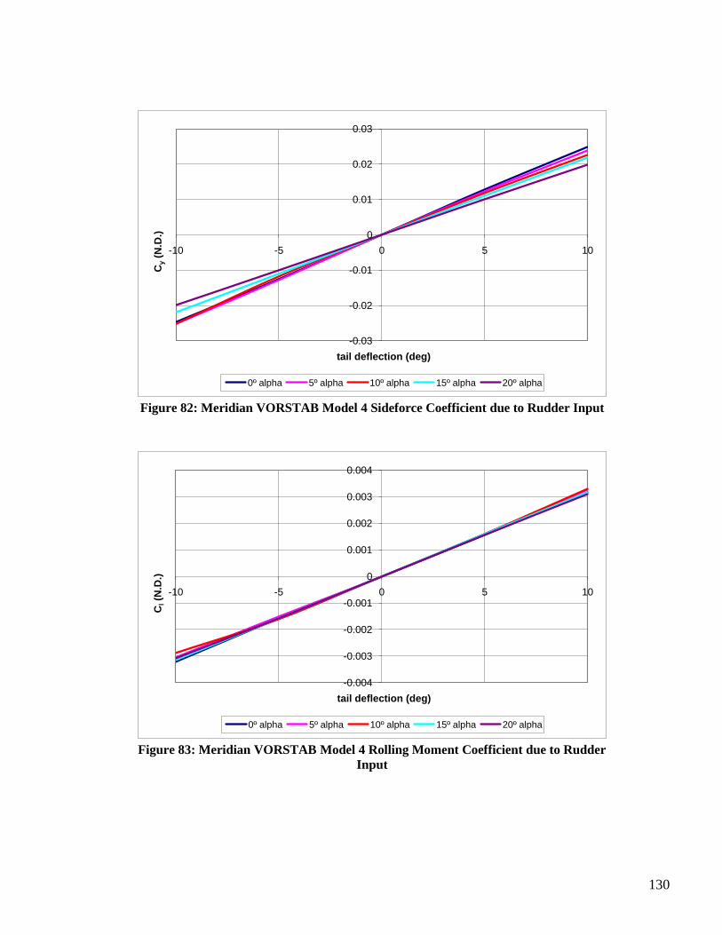
130

-0.03

-0.02

-0.01

0

0.01

0.02

0.03

-10 -5 0 5 10

Cy

(N.D

.)




-0.004

-0.003

-0.002

-0.001

0

0.001

0.002

0.003

0.004

-10 -5 0 5 10

Cl(N

.D.)




Input

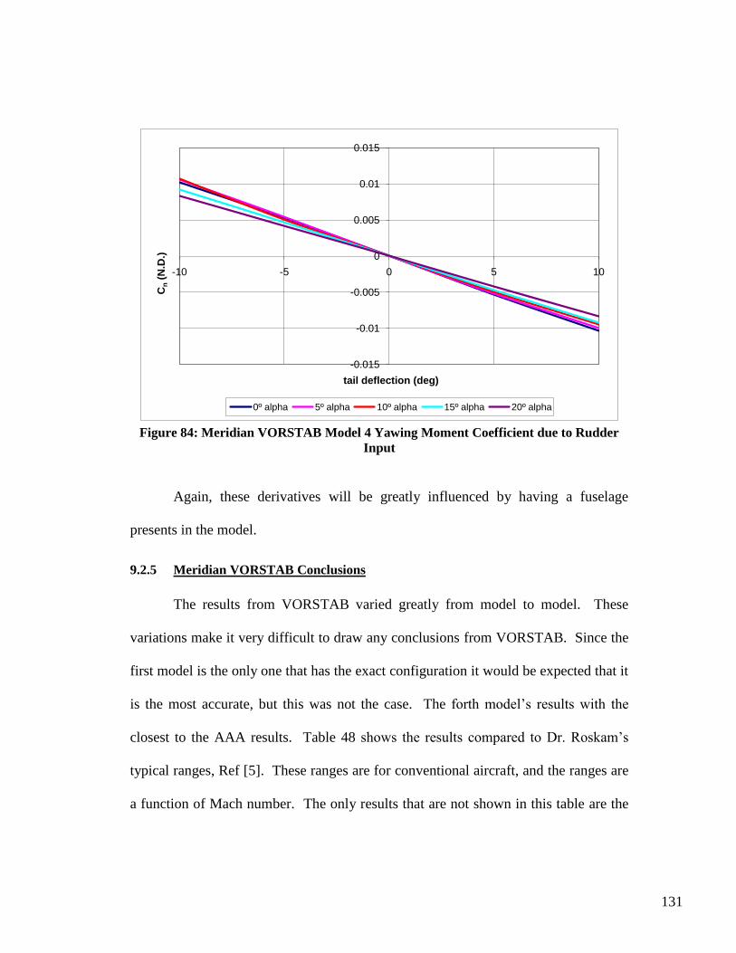
131

-0.015

-0.01

-0.005

0

0.005

0.01

0.015

-10 -5 0 5 10

Cn

(N.D

.)




Input

Again, these derivatives will be greatly influenced by having a fuselage

presents in the model.

9.2.5 Meridian VORSTAB Conclusions

The results from VORSTAB varied greatly from model to model. These

variations make it very difficult to draw any conclusions from VORSTAB. Since the

first model is the only one that has the exact configuration it would be expected that it

is the most accurate, but this was not the case. The forth model‟s results with the

closest to the AAA results. Table 48 shows the results compared to Dr. Roskam‟s

typical ranges, Ref [5]. These ranges are for conventional aircraft, and the ranges are

a function of Mach number. The only results that are not shown in this table are the

132

first model. Model 1‟s results were not valid at all, so they were completely ignored.

The first model was used as a stepping stone to create the other models.

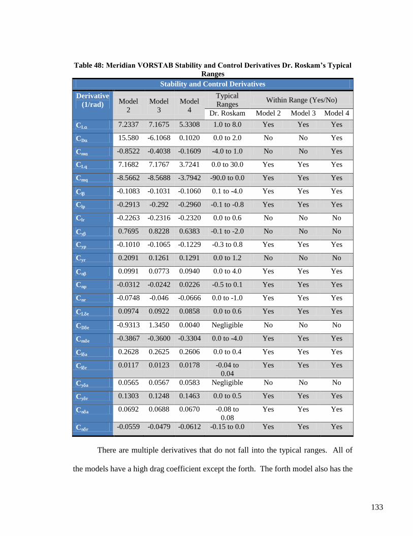
133

Table 48: Meridian VORSTAB Stability and Control Derivatives Dr. Roskam’s Typical

Ranges


Derivative

(1/rad) Model

2

Model

3

Model

4

Typical

Ranges Within Range (Yes/No)

Dr. Roskam Model 2 Model 3 Model 4

CL 7.2337 7.1675 5.3308 1.0 to 8.0 Yes Yes Yes

CD 15.580 -6.1068 0.1020 0.0 to 2.0 No No Yes

Cm -0.8522 -0.4038 -0.1609 -4.0 to 1.0 No No Yes

CLq 7.1682 7.1767 3.7241 0.0 to 30.0 Yes Yes Yes

Cmq -8.5662 -8.5688 -3.7942 -90.0 to 0.0 Yes Yes Yes

Cl -0.1083 -0.1031 -0.1060 0.1 to -4.0 Yes Yes Yes

Clp -0.2913 -0.292 -0.2960 -0.1 to -0.8 Yes Yes Yes

Clr -0.2263 -0.2316 -0.2320 0.0 to 0.6 No No No

Cy 0.7695 0.8228 0.6383 -0.1 to -2.0 No No No

Cyp -0.1010 -0.1065 -0.1229 -0.3 to 0.8 Yes Yes Yes

Cyr 0.2091 0.1261 0.1291 0.0 to 1.2 No No No

Cn 0.0991 0.0773 0.0940 0.0 to 4.0 Yes Yes Yes

Cnp -0.0312 -0.0242 0.0226 -0.5 to 0.1 Yes Yes Yes

Cnr -0.0748 -0.046 -0.0666 0.0 to -1.0 Yes Yes Yes

CLe 0.0974 0.0922 0.0858 0.0 to 0.6 Yes Yes Yes

CDe -0.9313 1.3450 0.0040 Negligible No No No

Cme -0.3867 -0.3600 -0.3304 0.0 to -4.0 Yes Yes Yes

Cla 0.2628 0.2625 0.2606 0.0 to 0.4 Yes Yes Yes

Clr 0.0117 0.0123 0.0178 -0.04 to

0.04

Yes Yes Yes

Cya 0.0565 0.0567 0.0583 Negligible No No No

Cyr 0.1303 0.1248 0.1463 0.0 to 0.5 Yes Yes Yes

Cna 0.0692 0.0688 0.0670 -0.08 to

0.08

Yes Yes Yes

Cnr -0.0559 -0.0479 -0.0612 -0.15 to 0.0 Yes Yes Yes

There are multiple derivatives that do not fall into the typical ranges. All of

the models have a high drag coefficient except the forth. The forth model also has the

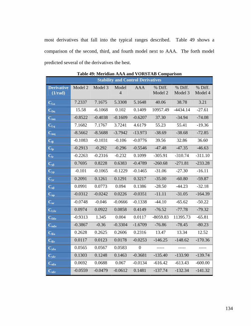
134

most derivatives that fall into the typical ranges described. Table 49 shows a

comparison of the second, third, and fourth model next to AAA. The forth model

predicted several of the derivatives the best.

Table 49: Meridian AAA and VORSTAB Comparison


Derivative

(1/rad)

Model 2 Model 3 Model

4

AAA % Diff.

Model 2

% Diff.

Model 3

% Diff.

Model 4

CL 7.2337 7.1675 5.3308 5.1648 40.06 38.78 3.21

CD 15.58 -6.1068 0.102 0.1409 10957.49 -4434.14 -27.61

Cm -0.8522 -0.4038 -0.1609 -0.6207 37.30 -34.94 -74.08

CLq 7.1682 7.1767 3.7241 4.6179 55.23 55.41 -19.36

Cmq -8.5662 -8.5688 -3.7942 -13.973 -38.69 -38.68 -72.85

Cl -0.1083 -0.1031 -0.106 -0.0776 39.56 32.86 36.60

Clp -0.2913 -0.292 -0.296 -0.5546 -47.48 -47.35 -46.63

Clr -0.2263 -0.2316 -0.232 0.1099 -305.91 -310.74 -311.10

Cy 0.7695 0.8228 0.6383 -0.4789 -260.68 -271.81 -233.28

Cyp -0.101 -0.1065 -0.1229 -0.1465 -31.06 -27.30 -16.11

Cyr 0.2091 0.1261 0.1291 0.3217 -35.00 -60.80 -59.87

Cn 0.0991 0.0773 0.094 0.1386 -28.50 -44.23 -32.18

Cnp -0.0312 -0.0242 0.0226 -0.0351 -11.11 -31.05 -164.39

Cnr -0.0748 -0.046 -0.0666 -0.1338 -44.10 -65.62 -50.22

CLe 0.0974 0.0922 0.0858 0.4149 -76.52 -77.78 -79.32

CDe -0.9313 1.345 0.004 0.0117 -8059.83 11395.73 -65.81

Cme -0.3867 -0.36 -0.3304 -1.6709 -76.86 -78.45 -80.23

Cla 0.2628 0.2625 0.2606 0.2316 13.47 13.34 12.52

Clr 0.0117 0.0123 0.0178 -0.0253 -146.25 -148.62 -170.36

Cya 0.0565 0.0567 0.0583 0 ----- ----- -----

Cyr 0.1303 0.1248 0.1463 -0.3681 -135.40 -133.90 -139.74

Cna 0.0692 0.0688 0.067 -0.0134 -616.42 -613.43 -600.00

Cnr -0.0559 -0.0479 -0.0612 0.1481 -137.74 -132.34 -141.32

135

The fourth model best predicted the Meridian stability and control derivatives

when compared to AAA. There are several derivatives that are extremely far off, but

the fuselage will have an impact on most of these. After modeling these three

different aircraft it can be concluded that VORSTAB works best with traditional style

aircraft, such as the YAK-54. The Meridian is not a typical style of aircraft and the

VORSTAB results were not what were expected. These results should not be

completely ignored, because they brought up possible issues that the Meridian might

have. For example, the downward swoop of the fuselage could result in downwash

and flow separation. This downwash and flow separation possible could render the

tails ineffective and the aircraft unresponsive to tail inputs. It is recommended that

several more wing and tail models be created to determine if it predicts the stability

and control derivatives well as seen from the Meridian results.

9.3 Linearized Model of the Meridian

For the information and data on the state space model of the Meridian please

refer to Appendix B.

9.4 FLUENT Modeling of the Meridian

As learned from the VORSTAB model of the Meridian, the main concern is the

downwash created over the fuselage that could blank out the v-tails. The first flight

tests also resulted in very high drag. These two problems, downwash and drag, drove

the need for a FLUENT model to be created. A 3-D model was desired, but due to

time constraints this was not done. Therefore, a 2-D side profile of the fuselage was

136

created to see the downwash that was produced from the high camber. A complete 3-

D model of the Meridian should eventually be created.

9.4.1 GAMBIT Mesh Generation

A large farfield was created around the axial-crosscut of the fuselage. The

farfield was broken into six individual sections; forward (above and below) of the

fuselage, aft (above and below) of the fuselage, above the fuselage, and below the

fuselage. Above and below the fuselage had a height of 20 maximum thicknesses of

the fuselage, and forward and aft had a length of 20 lengths of the fuselage. This

created a large enough area where the flow could be appropriately modeled. The size

of the farfields depends on the flow being modeled and the shape of the object. A

very fine mesh is desirable everywhere, but this would take a large amount of

computer memory and time to run. Different farfields allow the designer to create

finer meshes in the more critical sections of the flow. For the 2-D Meridian fuselage

the critical flow section was the boundary layer of the Meridian walls. This is where

the flow can separate. The flow at a large distance from the fuselage is not as critical

as the flow near the walls. The following are the steps taken to create the six farfields

and their meshes:

Step 1: Import the axial cross-section of the fuselage (points created as a text file).

The tip of the nose will be on the (0, 0, 0) point. Figure 85 shows the Meridian cross-

section.

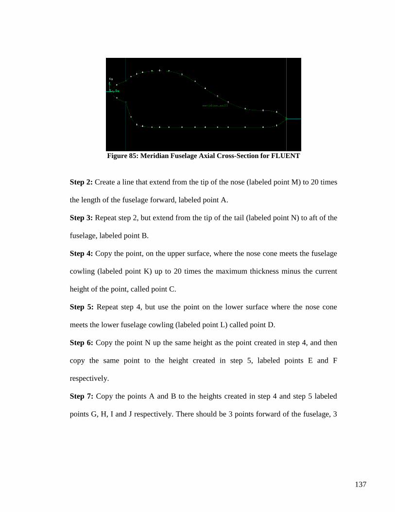
137

Figure 85: Meridian Fuselage Axial Cross-Section for FLUENT

Step 2: Create a line that extend from the tip of the nose (labeled point M) to 20 times

the length of the fuselage forward, labeled point A.

Step 3: Repeat step 2, but extend from the tip of the tail (labeled point N) to aft of the

fuselage, labeled point B.

Step 4: Copy the point, on the upper surface, where the nose cone meets the fuselage

cowling (labeled point K) up to 20 times the maximum thickness minus the current

height of the point, called point C.

Step 5: Repeat step 4, but use the point on the lower surface where the nose cone

meets the lower fuselage cowling (labeled point L) called point D.

Step 6: Copy the point N up the same height as the point created in step 4, and then

copy the same point to the height created in step 5, labeled points E and F

respectively.

Step 7: Copy the points A and B to the heights created in step 4 and step 5 labeled

points G, H, I and J respectively. There should be 3 points forward of the fuselage, 3

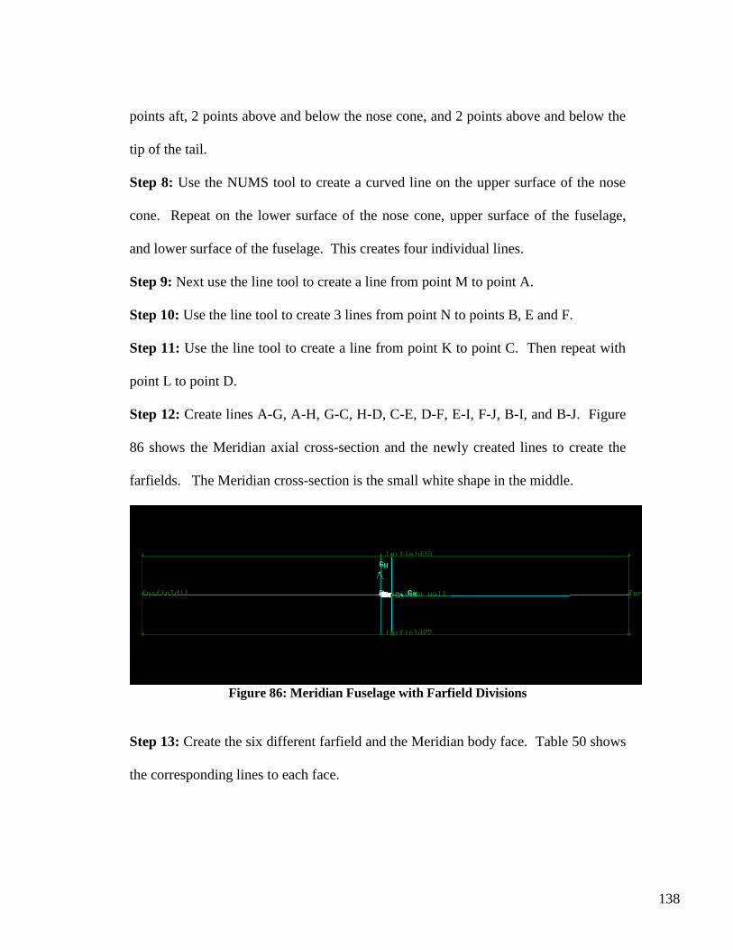
138

points aft, 2 points above and below the nose cone, and 2 points above and below the

tip of the tail.

Step 8: Use the NUMS tool to create a curved line on the upper surface of the nose

cone. Repeat on the lower surface of the nose cone, upper surface of the fuselage,

and lower surface of the fuselage. This creates four individual lines.

Step 9: Next use the line tool to create a line from point M to point A.

Step 10: Use the line tool to create 3 lines from point N to points B, E and F.

Step 11: Use the line tool to create a line from point K to point C. Then repeat with

point L to point D.

Step 12: Create lines A-G, A-H, G-C, H-D, C-E, D-F, E-I, F-J, B-I, and B-J. Figure

86 shows the Meridian axial cross-section and the newly created lines to create the

farfields. The Meridian cross-section is the small white shape in the middle.

Figure 86: Meridian Fuselage with Farfield Divisions

Step 13: Create the six different farfield and the Meridian body face. Table 50 shows

the corresponding lines to each face.

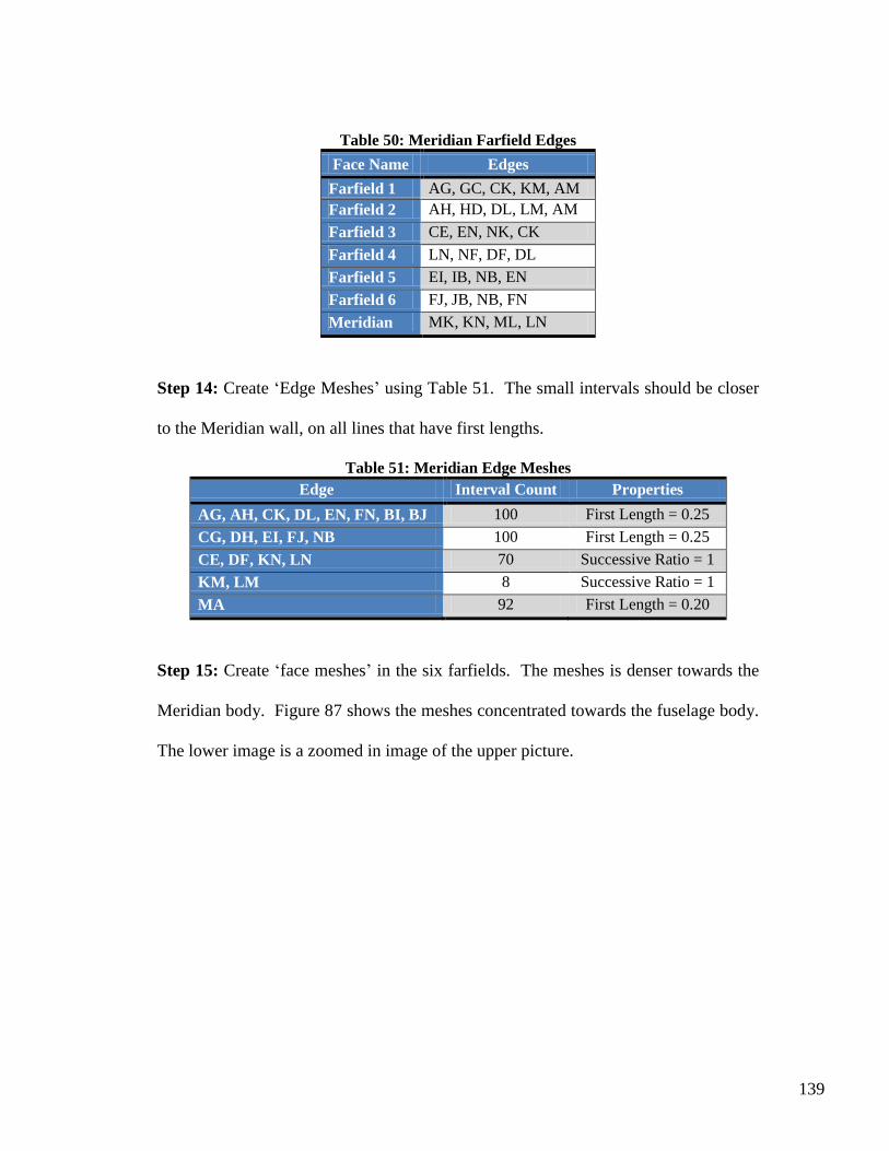
139

Table 50: Meridian Farfield Edges

Face Name Edges

Farfield 1 AG, GC, CK, KM, AM

Farfield 2 AH, HD, DL, LM, AM

Farfield 3 CE, EN, NK, CK

Farfield 4 LN, NF, DF, DL

Farfield 5 EI, IB, NB, EN

Farfield 6 FJ, JB, NB, FN

Meridian MK, KN, ML, LN

Step 14: Create „Edge Meshes‟ using Table 51. The small intervals should be closer

to the Meridian wall, on all lines that have first lengths.

Table 51: Meridian Edge Meshes

Edge Interval Count Properties

AG, AH, CK, DL, EN, FN, BI, BJ 100 First Length = 0.25

CG, DH, EI, FJ, NB 100 First Length = 0.25

CE, DF, KN, LN 70 Successive Ratio = 1

KM, LM 8 Successive Ratio = 1

MA 92 First Length = 0.20

Step 15: Create „face meshes‟ in the six farfields. The meshes is denser towards the

Meridian body. Figure 87 shows the meshes concentrated towards the fuselage body.

The lower image is a zoomed in image of the upper picture.

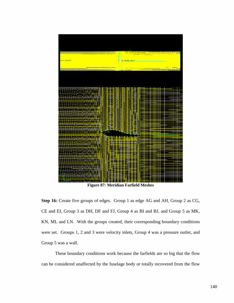
140

Figure 87: Meridian Farfield Meshes

Step 16: Create five groups of edges. Group 1 as edge AG and AH, Group 2 as CG,

CE and EI, Group 3 as DH, DF and FJ, Group 4 as BI and BJ, and Group 5 as MK,

KN, ML and LN. With the groups created, their corresponding boundary conditions

were set. Groups 1, 2 and 3 were velocity inlets, Group 4 was a pressure outlet, and

Group 5 was a wall.

These boundary conditions work because the farfields are so big that the flow

can be considered unaffected by the fuselage body or totally recovered from the flow

141

disturbances. The boundary conditions can be modified in FLUENT if they are not

what were desired. With the GAMBIT model fully created export the 2-D mesh and

import it into FLUENT.

9.5 FLUENT Model Generation

The FLUENT model can be run in many different methods depending on what

the goals the designer is trying to achieve. For the Meridian, the goal was to observe

the boundary layer on the fuselage, and observe the flow separation and/or downwash

that were produced from the high convergence and downward camber. Several

different turbulent methods were tested to verify which one was the most accurate.

For the Meridian, the results did not very greatly from one method to the next.

Therefore, the method chosen was the one that has the most accurate results in

aerodynamics. The following are the setup criteria for the FLUENT model.

Solver – Segregated, because of limited memory

Viscous – Turbulent, Spalart-Allmaras; set the turbulence factors to 0.1 for an

initial guess.

No Energy Equation because the flow is not compressible

Materials – Set the density and viscosity to the values that the Meridian will

fly in. At 1,000 m the approximate values are 1.112 kg/m3 and 1.758x10

-5

kg/m-s respectively.

Operating Conditions – Set this to zero to work in terms of absolute pressure.

If left at the default setting the pressures reported would be in terms of gauge

pressure.

142

Boundary Conditions – The types of boundary conditions chosen in GAMBIT

were the desired ones for this model, but the values had to set.

o Velocity Inlets – 61.7 m/s in the x-direction and 0.0 m/s in the y-

direction. For angles of attack the velocity components could be

changed. The model did not converge doing this, so a new mesh was

created for each angle of attack chosen. To create the new mesh the

same method as before was used, but the imported Meridian cross-

section was imported at the correct angle of attack.

o Pressure Outlet – 0 Pascals for the gauge pressure

o Wall – Set the wall roughness height to 3x10-5

m and roughness

constant to 0.5. These were the values used by AAA when designing

the aircraft.

Solution – SIMPLE for the pressure-velocity coupling, PRESTO! for the

pressure discretization, and Second-Order Upwind for the other

discretizations. These were determined using the online FLUENT help, Ref

[19].

Residuals – 1x10-6

Monitor – Lift and drag

Iterate until converged

The mesh generation and FLUENT runs were repeated for several different

angles of attack. Multiple angles of attack allow the designer to see the changes in

the flow as the aircraft body changes orientation.

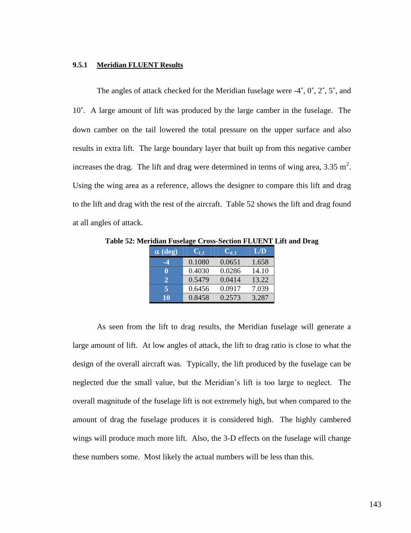
143

9.5.1 Meridian FLUENT Results

The angles of attack checked for the Meridian fuselage were -4˚, 0˚, 2˚, 5˚, and

10˚. A large amount of lift was produced by the large camber in the fuselage. The

down camber on the tail lowered the total pressure on the upper surface and also

results in extra lift. The large boundary layer that built up from this negative camber

increases the drag. The lift and drag were determined in terms of wing area, 3.35 m2.

Using the wing area as a reference, allows the designer to compare this lift and drag

to the lift and drag with the rest of the aircraft. Table 52 shows the lift and drag found

at all angles of attack.

Table 52: Meridian Fuselage Cross-Section FLUENT Lift and Drag

(deg) Cl_f Cd_f L/D

-4 0.1080 0.0651 1.658

0 0.4030 0.0286 14.10

2 0.5479 0.0414 13.22

5 0.6456 0.0917 7.039

10 0.8458 0.2573 3.287

As seen from the lift to drag results, the Meridian fuselage will generate a

large amount of lift. At low angles of attack, the lift to drag ratio is close to what the

design of the overall aircraft was. Typically, the lift produced by the fuselage can be

neglected due the small value, but the Meridian‟s lift is too large to neglect. The

overall magnitude of the fuselage lift is not extremely high, but when compared to the

amount of drag the fuselage produces it is considered high. The highly cambered

wings will produce much more lift. Also, the 3-D effects on the fuselage will change

these numbers some. Most likely the actual numbers will be less than this.

144

The FLUENT results can best be shown in the form of pictures. The

downwash, flow separation, and boundary layer can all easy be seen in the velocity

magnitude, velocity angle, total pressure, stream function, vorticity profiles. Figure

88 shows the velocity magnitude of the air around the Meridian. From left to right,

top to bottom the figures are in an order of 0˚, 2˚, 5˚, 10˚, and -4˚.

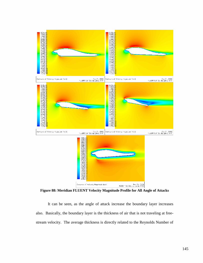
145

Figure 88: Meridian FLUENT Velocity Magnitude Profile for All Angle of Attacks

It can be seen, as the angle of attack increase the boundary layer increases

also. Basically, the boundary layer is the thickness of air that is not traveling at free-

stream velocity. The average thickness is directly related to the Reynolds Number of

146

the flow and the length of the surface. A Cartesian coordinate system is used for the

boundary layer definitions. The x-coordinate is parallel with the surface at each

point, and the y-coordinate is normal to the surface. Eq [28] shows an estimate for

the average thickness of the boundary layer, and Eq [29] show the definition of

Reynolds Number, Ref [20].

Eq [28]

Eq [29]

There are three common measurements of the boundary layer thickness, .

One method is defined as the distance from the wall where the velocity reaches 99

percent of the free stream velocity, u = 0.99U. This method is somewhat arbitrary

since any percentage could have been picked. The reason 100 percent of the free

stream velocity was not chosen is that it is difficult to pinpoint the exact location

where this happens. It is appropriate to assume 99 percent is close enough for

accuracy. The second method is the displacement thickness, *, and there is no

arbitrariness in this method. Displacement thickness is the theoretical distance that

the wall would have to move outward, in a frictionless flow, to maintain the same

mass flux as the authentic flow. Eq [30] shows the displacement thickness, Ref [20].

The upper boundary goes to infinity, because u/U goes to 0 exponentially fast in the y

direction, as y goes to infinity.

Eq [30]

o “u” is a function of the variable “y”.

147

The third method is the momentum thickness, , and is defined as the amount

of momentum, U2, loss due to the boundary layer. This momentum thickness can

be determined using Eq [31], Ref [20]. Again in this equation “u” is a function of

the variable “y”.

Eq [31]

The type of definition does not matter when it comes to boundary layer. Each

method has its benefits and downfalls. For example, the second and third methods

are difficult to develop an equation for the velocity, u. As stated earlier the first

method chooses an arbitrary number, but this is the easiest to use with experimental

data. FLUENT depicts the velocity magnitude by varying the color. This is depicted

by the blue area around the fuselage. The boundary layer flow stays attached to the

fuselage and follows the contour of it. Boundary layers will build up in the y-

direction as the flow travels over the body. The size of the boundary layer is

extremely thick at high angles of attack. For a typical aircraft wing the boundary

layer thickness is on the order of one centimeter. At higher angles of attack, 5˚ and

10˚, and large fuselage curvatures the flow separates completely from the fuselage.

This is seen as the blue area that does not follow the fuselage contour, but instead

starts flowing turbulently. The direction of the flow can be shown by viewing the

velocity angle in Figure 89. The orientation of the angles is 0˚ to the right and 90˚

straight up.

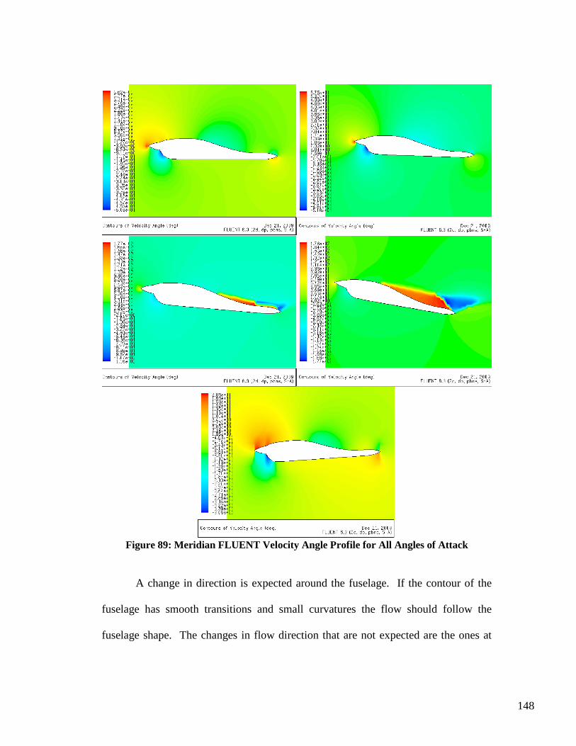
148

Figure 89: Meridian FLUENT Velocity Angle Profile for All Angles of Attack

A change in direction is expected around the fuselage. If the contour of the

fuselage has smooth transitions and small curvatures the flow should follow the

fuselage shape. The changes in flow direction that are not expected are the ones at

149

angles of attack 5˚ and 10˚. Separation occurs at these angles of attack near the

empennage. Similar to the velocity magnitude, the velocity angle depicts its changes

with changes in color. A smooth change is depicted with a slow transition in color,

and a sudden change with a dramatic change in color. This separation bubble is

where the flow can travel in many directions and possible have complete flow

reversal. The direction of the velocity for angles of attack -4˚, 0˚, and 2˚ follows the

contour of the fuselage pretty well. There are a few sudden changes, but this is

expected when the flow encounters a disturbance in the path. For example, the flow

changes direction abruptly at the nose cone of the aircraft. The flow stops at this

point and begins to travel around that spot.

At higher angles of attack, 5˚ and 10˚, there are unexpected turns in the flow.

The pressure gradient along the surface determines how the flow travels over a

surface. A favorable pressure gradient will be upstream of the highest point, and this

will cause the streamlines of the flow to converge and a decrease in pressure. An

adverse pressure gradient is the opposite of the favorable pressure gradient.

Downstream of the highest point the streamlines diverge and result in an increase in

pressure. These pressure gradients not only affect the pressure, but also the velocity.

A favorable pressure gradient will increase the free stream velocity, and an adverse

pressure gradient will decrease the free stream velocity. Figure 90 depicts the

velocity profiles along a curved surface, Ref [20].

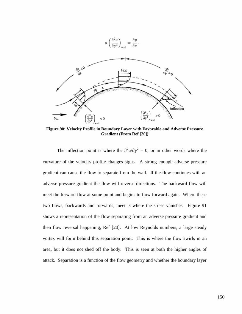
150

Figure 90: Velocity Profile in Boundary Layer with Favorable and Adverse Pressure

Gradient (From Ref [20])

The inflection point is where the 2u/y

2 = 0, or in other words where the

curvature of the velocity profile changes signs. A strong enough adverse pressure

gradient can cause the flow to separate from the wall. If the flow continues with an

adverse pressure gradient the flow will reverse directions. The backward flow will

meet the forward flow at some point and begins to flow forward again. Where these

two flows, backwards and forwards, meet is where the stress vanishes. Figure 91

shows a representation of the flow separating from an adverse pressure gradient and

then flow reversal happening, Ref [20]. At low Reynolds numbers, a large steady

vortex will form behind this separation point. This is where the flow swirls in an

area, but it does not shed off the body. This is seen at both the higher angles of

attack. Separation is a function of the flow geometry and whether the boundary layer

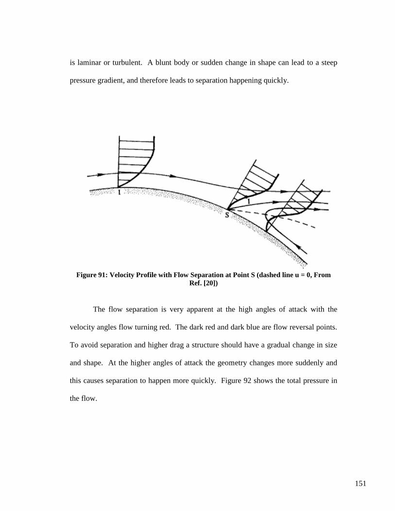
151

is laminar or turbulent. A blunt body or sudden change in shape can lead to a steep

pressure gradient, and therefore leads to separation happening quickly.

Figure 91: Velocity Profile with Flow Separation at Point S (dashed line u = 0, From

Ref. [20])

The flow separation is very apparent at the high angles of attack with the

velocity angles flow turning red. The dark red and dark blue are flow reversal points.

To avoid separation and higher drag a structure should have a gradual change in size

and shape. At the higher angles of attack the geometry changes more suddenly and

this causes separation to happen more quickly. Figure 92 shows the total pressure in

the flow.

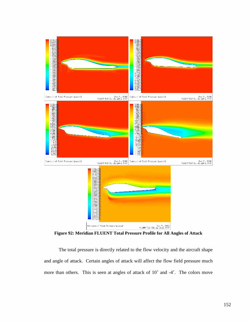
152

Figure 92: Meridian FLUENT Total Pressure Profile for All Angles of Attack

The total pressure is directly related to the flow velocity and the aircraft shape

and angle of attack. Certain angles of attack will affect the flow field pressure much

more than others. This is seen at angles of attack of 10˚ and -4˚. The colors move

153

away from the red color to a yellow or orange color. These changes in color are a

reduction in the total pressure due to the fuselage contour and flow velocity. This is

one of the reasons for the very low lift to drag ratio at these two angles of attack. The

total pressure is lower where the boundary layer is located and the where the flow

separates from the body due to the small velocity. Total pressure is a function of the

velocity squared, Eq [32].

Eq [32]

At the -4˚ angle of attack the boundary layer on the lower surface is very

thick. This is due to the sudden change in shape on the cowling. It is similar to the

flow encountering a step, and this causes the flow to separate very quickly. The flow

path can be seen in Figure 93 showing the stream functions. Stream functions have a

constant value along a streamline. These stream functions can be used to analytically

determine the velocity and its direction.

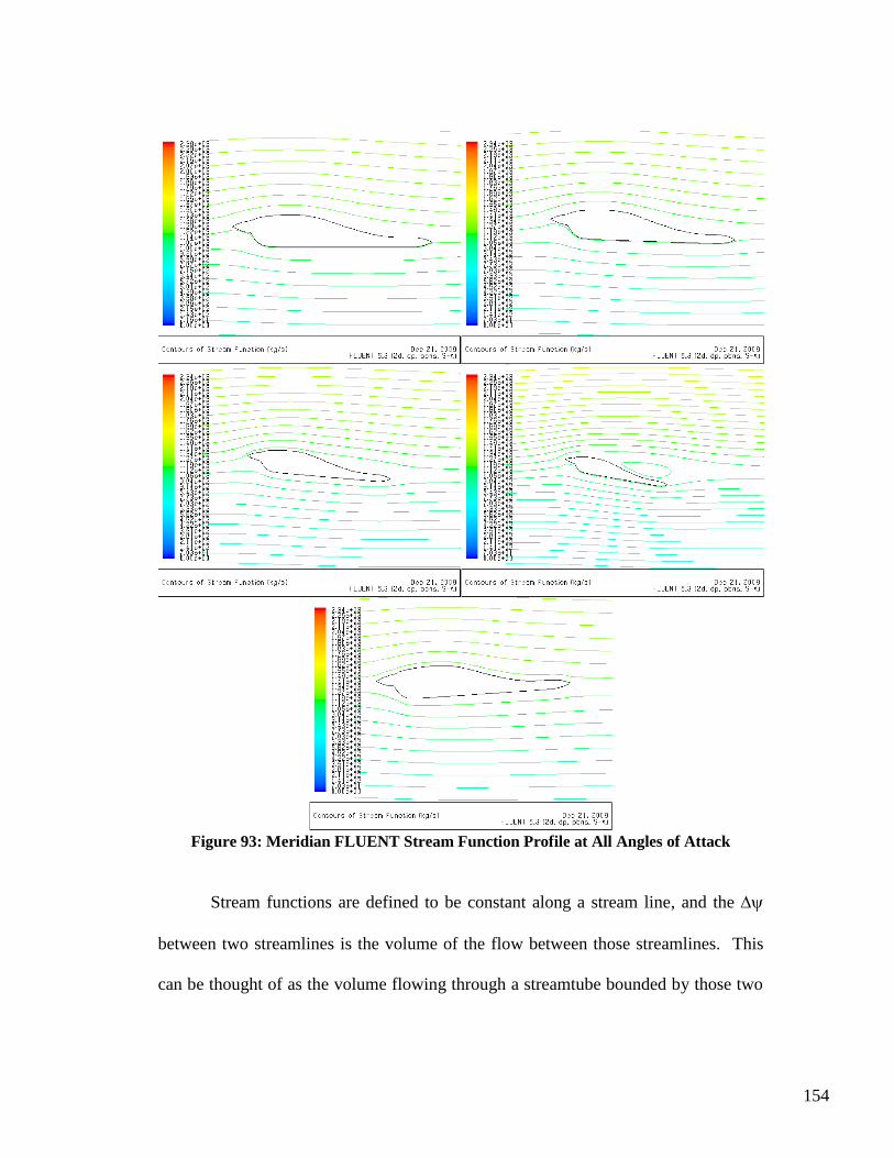
154

Figure 93: Meridian FLUENT Stream Function Profile at All Angles of Attack

Stream functions are defined to be constant along a stream line, and the

between two streamlines is the volume of the flow between those streamlines. This

can be thought of as the volume flowing through a streamtube bounded by those two

155

streamlines. The units for stream function are kg/s. A stream function normally has

units of kg/s-m, but this model is 2-D and has no depth. There is also a unitless form

of stream function and is defined by Eq [33] (without the bar), Ref [21]. To

determine the velocity components from the stream function Eq [34] and Eq [35]

should be used, Ref [21].

Eq [33]

Eq [34]

Eq [35]

At the high angle of attack, 10˚, it is seen that the stream function travels in a

complete closed path around the empennage. This is due to the flow separating from

the fuselage and traveling in this closed path. The rest of the flow travels over the top

of this circulation.

Vorticity is defined as twice the angular velocity, Ref [20]. This is found by

calculating the average rotation rate of two perpendicular lines and then multiplying it

by two. Irrotational flow will have a magnitude of zero vorticity. This is why the

dark blue area is very close to zero in Figure 94. There is high vorticity around the

abrupt curved spots on the fuselage. The boundary layer also is a lighter shade of

blue, because the flow in this area has rotation.

Using Stokes‟ theorem circulation can be written as Eq [36], Ref [20]. As

seen from this equation circulation is related to the rotation of the flow. Higher

angular velocity will produce more circulation around a finite area. Circulation can

be thought of as the strength of vorticity or vortex. Lift is related to circulation using

156

Eq [37], Ref [6]. This is known as the Kutta-Joukowski theorem. On most

computational fluid dynamics programs circulation is used as a step to calculate the

forces on a body. When a body is generating lift the circulation is finite. This means

that the lift is directly related to the boundary layer vorticity.

Eq [36]

Eq [37]

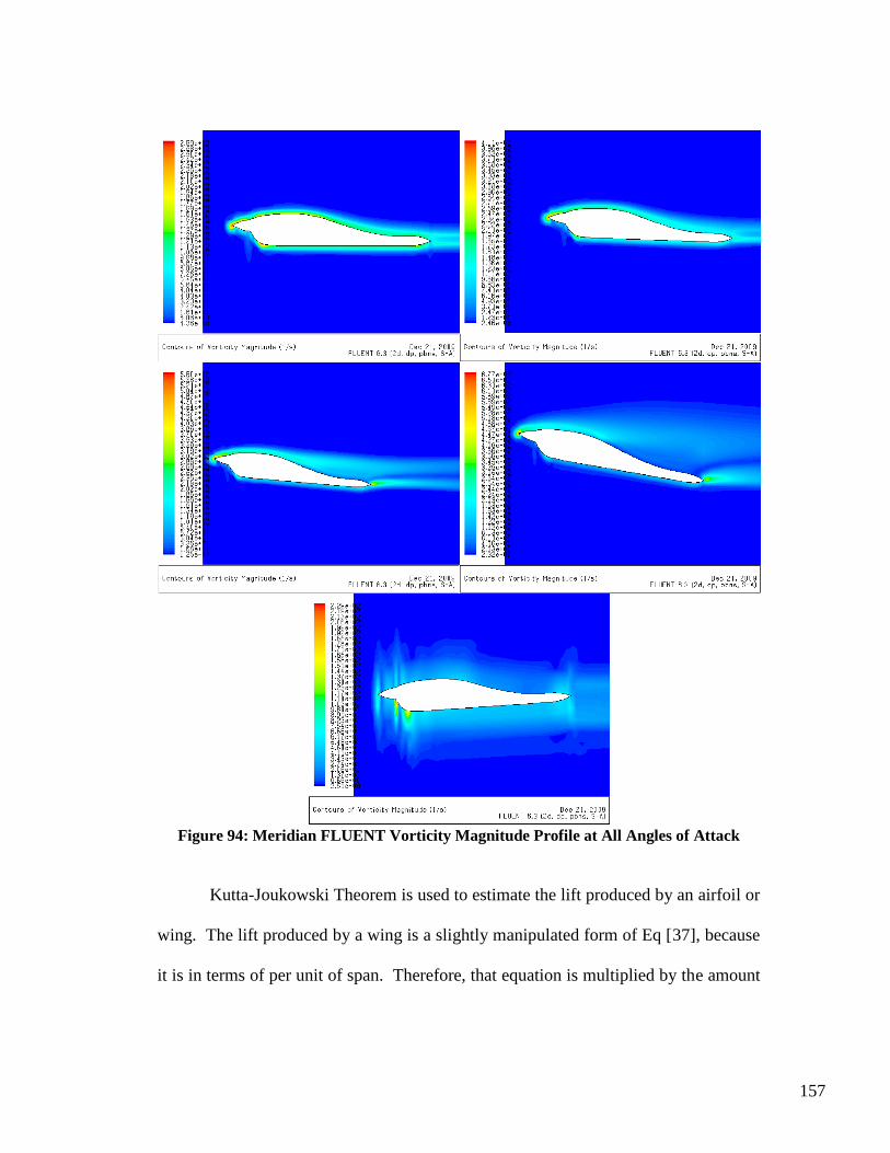
157

Figure 94: Meridian FLUENT Vorticity Magnitude Profile at All Angles of Attack

Kutta-Joukowski Theorem is used to estimate the lift produced by an airfoil or

wing. The lift produced by a wing is a slightly manipulated form of Eq [37], because

it is in terms of per unit of span. Therefore, that equation is multiplied by the amount

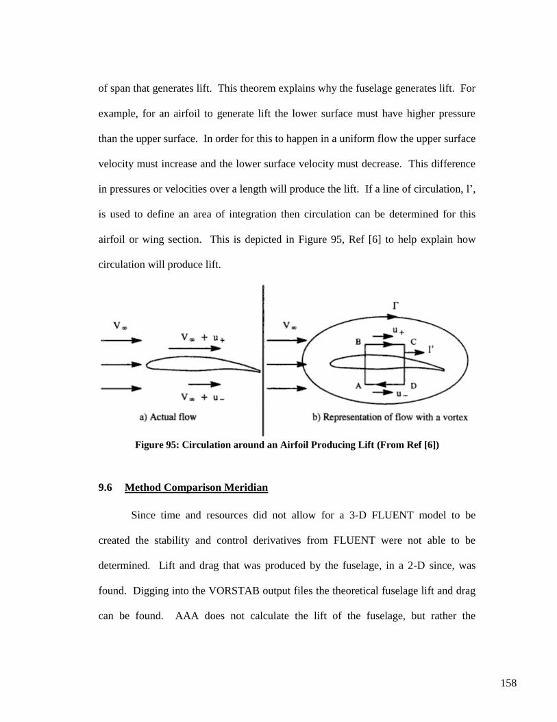
158

of span that generates lift. This theorem explains why the fuselage generates lift. For

example, for an airfoil to generate lift the lower surface must have higher pressure

than the upper surface. In order for this to happen in a uniform flow the upper surface

velocity must increase and the lower surface velocity must decrease. This difference

in pressures or velocities over a length will produce the lift. If a line of circulation, l‟,

is used to define an area of integration then circulation can be determined for this

airfoil or wing section. This is depicted in Figure 95, Ref [6] to help explain how

circulation will produce lift.

Figure 95: Circulation around an Airfoil Producing Lift (From Ref [6])

9.6 Method Comparison Meridian

Since time and resources did not allow for a 3-D FLUENT model to be

created the stability and control derivatives from FLUENT were not able to be

determined. Lift and drag that was produced by the fuselage, in a 2-D since, was

found. Digging into the VORSTAB output files the theoretical fuselage lift and drag

can be found. AAA does not calculate the lift of the fuselage, but rather the

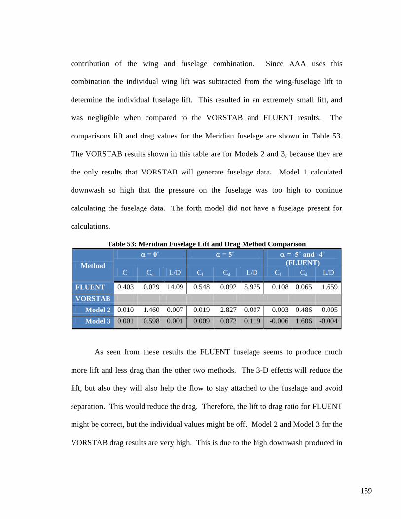
159

contribution of the wing and fuselage combination. Since AAA uses this

combination the individual wing lift was subtracted from the wing-fuselage lift to

determine the individual fuselage lift. This resulted in an extremely small lift, and

was negligible when compared to the VORSTAB and FLUENT results. The

comparisons lift and drag values for the Meridian fuselage are shown in Table 53.

The VORSTAB results shown in this table are for Models 2 and 3, because they are

the only results that VORSTAB will generate fuselage data. Model 1 calculated

downwash so high that the pressure on the fuselage was too high to continue

calculating the fuselage data. The forth model did not have a fuselage present for

calculations.

Table 53: Meridian Fuselage Lift and Drag Method Comparison

Method

= 0˚ = 5˚ = -5˚ and -4˚

(FLUENT)

Cl Cd L/D Cl Cd L/D Cl Cd L/D

FLUENT 0.403 0.029 14.09 0.548 0.092 5.975 0.108 0.065 1.659

VORSTAB

Model 2 0.010 1.460 0.007 0.019 2.827 0.007 0.003 0.486 0.005

Model 3 0.001 0.598 0.001 0.009 0.072 0.119 -0.006 1.606 -0.004

As seen from these results the FLUENT fuselage seems to produce much

more lift and less drag than the other two methods. The 3-D effects will reduce the

lift, but also they will also help the flow to stay attached to the fuselage and avoid

separation. This would reduce the drag. Therefore, the lift to drag ratio for FLUENT

might be correct, but the individual values might be off. Model 2 and Model 3 for the

VORSTAB drag results are very high. This is due to the high downwash produced in

160

by VORSTAB. Fuselages do not typically produce much lift. These VORSTAB lift

to drag ratios are nowhere near the expected value.

Similar to the YAK-54 and MantaHawk the stability and control derivatives

from both methods, VORSTAB and AAA, can be compared to one another. Table 54

shows the comparison for the Meridian stability and control derivatives.

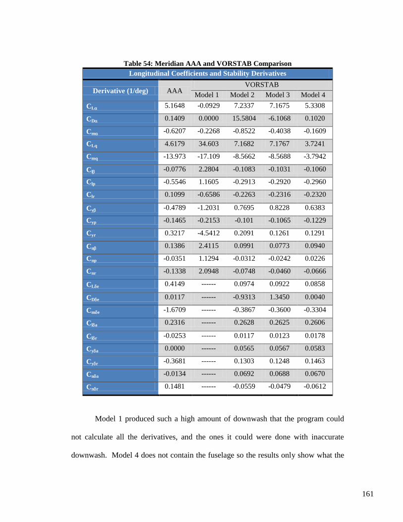
161

Table 54: Meridian AAA and VORSTAB Comparison

Longitudinal Coefficients and Stability Derivatives

Derivative (1/deg) AAA VORSTAB

Model 1 Model 2 Model 3 Model 4

CL 5.1648 -0.0929 7.2337 7.1675 5.3308

CD 0.1409 0.0000 15.5804 -6.1068 0.1020

Cm -0.6207 -0.2268 -0.8522 -0.4038 -0.1609

CLq 4.6179 34.603 7.1682 7.1767 3.7241

Cmq -13.973 -17.109 -8.5662 -8.5688 -3.7942

Cl -0.0776 2.2804 -0.1083 -0.1031 -0.1060

Clp -0.5546 1.1605 -0.2913 -0.2920 -0.2960

Clr 0.1099 -0.6586 -0.2263 -0.2316 -0.2320

Cy -0.4789 -1.2031 0.7695 0.8228 0.6383

Cyp -0.1465 -0.2153 -0.101 -0.1065 -0.1229

Cyr 0.3217 -4.5412 0.2091 0.1261 0.1291

Cn 0.1386 2.4115 0.0991 0.0773 0.0940

Cnp -0.0351 1.1294 -0.0312 -0.0242 0.0226

Cnr -0.1338 2.0948 -0.0748 -0.0460 -0.0666

CLe 0.4149 ------ 0.0974 0.0922 0.0858

CDe 0.0117 ------ -0.9313 1.3450 0.0040

Cme -1.6709 ------ -0.3867 -0.3600 -0.3304

Cla 0.2316 ------ 0.2628 0.2625 0.2606

Clr -0.0253 ------ 0.0117 0.0123 0.0178

Cya 0.0000 ------ 0.0565 0.0567 0.0583

Cyr -0.3681 ------ 0.1303 0.1248 0.1463

Cna -0.0134 ------ 0.0692 0.0688 0.0670

Cnr 0.1481 ------ -0.0559 -0.0479 -0.0612

Model 1 produced such a high amount of downwash that the program could

not calculate all the derivatives, and the ones it could were done with inaccurate

downwash. Model 4 does not contain the fuselage so the results only show what the

162

wings and v-tail produce in terms of stability and control derivatives. The

VORSTAB results are unstable in many different modes as discussed earlier and the

AAA results are stable in every mode.

The same typical ranges that applied to the YAK-54 and MantaHawk apply to

the Meridian as well. These ranges again were developed by Dr. Roskam, Ref [5] for

what a conventional aircraft can expect the control derivatives to be approximately.

These ranges are a function of Mach number. Table 55 shows the VORSTAB and

AAA Meridian results compared to typical ranges from Dr. Roskam, Ref [5].

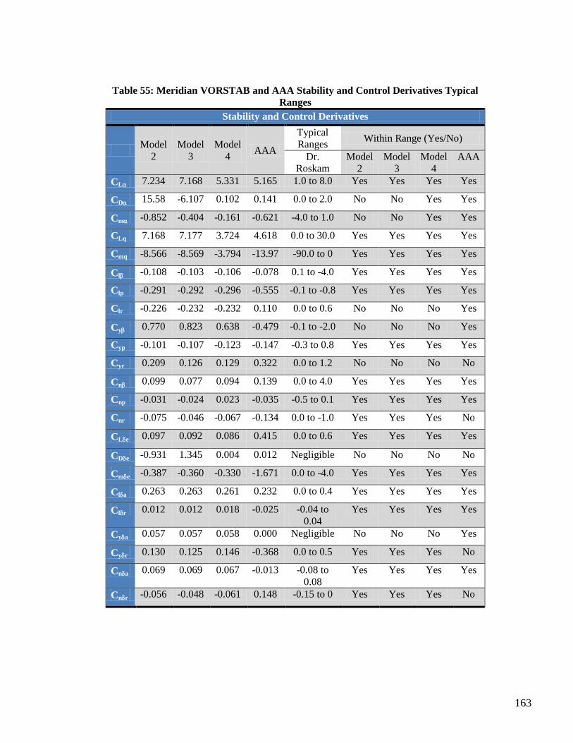
163

Table 55: Meridian VORSTAB and AAA Stability and Control Derivatives Typical

Ranges


Model

2

Model

3

Model

4 AAA

Typical

Ranges Within Range (Yes/No)

Dr.

Roskam

Model

2

Model

3

Model

4

AAA

CL 7.234 7.168 5.331 5.165 1.0 to 8.0 Yes Yes Yes Yes

CD 15.58 -6.107 0.102 0.141 0.0 to 2.0 No No Yes Yes

Cm -0.852 -0.404 -0.161 -0.621 -4.0 to 1.0 No No Yes Yes

CLq 7.168 7.177 3.724 4.618 0.0 to 30.0 Yes Yes Yes Yes

Cmq -8.566 -8.569 -3.794 -13.97 -90.0 to 0 Yes Yes Yes Yes

Cl -0.108 -0.103 -0.106 -0.078 0.1 to -4.0 Yes Yes Yes Yes

Clp -0.291 -0.292 -0.296 -0.555 -0.1 to -0.8 Yes Yes Yes Yes

Clr -0.226 -0.232 -0.232 0.110 0.0 to 0.6 No No No Yes

Cy 0.770 0.823 0.638 -0.479 -0.1 to -2.0 No No No Yes

Cyp -0.101 -0.107 -0.123 -0.147 -0.3 to 0.8 Yes Yes Yes Yes

Cyr 0.209 0.126 0.129 0.322 0.0 to 1.2 No No No No

Cn 0.099 0.077 0.094 0.139 0.0 to 4.0 Yes Yes Yes Yes

Cnp -0.031 -0.024 0.023 -0.035 -0.5 to 0.1 Yes Yes Yes Yes

Cnr -0.075 -0.046 -0.067 -0.134 0.0 to -1.0 Yes Yes Yes No

CLe 0.097 0.092 0.086 0.415 0.0 to 0.6 Yes Yes Yes Yes

CDe -0.931 1.345 0.004 0.012 Negligible No No No No

Cme -0.387 -0.360 -0.330 -1.671 0.0 to -4.0 Yes Yes Yes Yes

Cla 0.263 0.263 0.261 0.232 0.0 to 0.4 Yes Yes Yes Yes

Clr 0.012 0.012 0.018 -0.025 -0.04 to

0.04

Yes Yes Yes Yes

Cya 0.057 0.057 0.058 0.000 Negligible No No No Yes

Cyr 0.130 0.125 0.146 -0.368 0.0 to 0.5 Yes Yes Yes No

Cna 0.069 0.069 0.067 -0.013 -0.08 to

0.08

Yes Yes Yes Yes

Cnr -0.056 -0.048 -0.061 0.148 -0.15 to 0 Yes Yes Yes No

164

As seen from the table not all of the control derivatives fall within the typical

ranges. This does not necessarily mean that the aircraft is unstable. The rudder input

is a symmetrical deflection of the v-tail and unsymmetrical deflection is an elevator

input. In some cases the AAA results do not fall into the expected range, but the

VORSTAB results do. This does not mean that VORSTAB was correct in that case

and that AAA was incorrect. The Meridian might just have higher values in some

derivatives than a typical aircraft has.

From these results it can be determined that VORSTAB is most affective with

less complex aircraft. The Meridian was very difficult to model and achieve accurate

results. This does not mean that VORSTAB is not a high fidelity tool or inaccurate,

but rather should be used on aircraft that have a simpler design. The fuselage model

was changed many times until results that were closer to the desired results were

achieved. Basically it was very similar to guessing and checking. This is not

necessarily bad, because many times the meshes of a FLUENT model have to be

remade until the results are what was desired or expected. It is very difficult to

determine if these programs are producing the correct results without comparing their

results with actual fight tests. After that comparison one can draw a better conclusion

about the validity of the results.

165

10 Conclusions and Recommendations

After analyzing the three aircraft with AAA and VORSTAB conclusions

about both software programs were drawn. AAA is a valid method for quickly

estimating the stability and control derivatives, even at a low Reynolds number. It is

a rather affordable software program and easy to use. A downfall to the program is

that a low fidelity method is used to derive the derivatives. A downfall of VORSTAB

is that it is very difficult to make a VORSTAB model and requires someone with

experience or guidance. The VORSTAB model also takes a considerable longer

amount of time to create than AAA. VORSTAB uses a high fidelity method to derive

the stability and control derivatives. For low Reynolds number, AAA overestimates

estimates the drag and this was one of the main reason that a VORSTAB model was

created for all of the vehicles. These are the obvious downfalls and benefits to both

programs.

For the YAK-54, VORSTAB showed that the drag, CDo, was lower than AAA

predicted, as expected. This is a major advantage of VORSTAB is that the drag

estimation is closer to the actual drag. From the flight test data, VORSTAB estimated

many derivatives better than the AAA program did. Some of the derivatives from

VORSTAB are obvious that they are wrong and these should be ignored. For

example, the yawing moment due to aileron deflection has results that are not

symmetric, but opposite, for positive and negative aileron deflections. It is known

that a positive and negative aileron deflection should result in the same magnitude for

this derivative. These improvements from VORSTAB can be significant in creating a

166

valid YAK-54 model. From these results, both software programs are a valid

engineering tool and both should be used for deriving the derivatives.

Similar to the YAK-54, VORSTAB predicted a lower drag than AAA for the

MantaHawk. Without flight test it cannot be determined if VORSTAB or AAA

predicted the drag best. The MantaHawk wrecked early into the first flight test and

hardly any data was collected. From the small amount of data and explanation from

the flight test team the vehicle wrecked from a pitching moment error. AAA did not

predict this problem and said the vehicle should be stable in all modes. Most of

AAA‟s data is based on conventional aircraft and not a flying wing. VORSTAB

predicted that the MantaHawk was stable in every mode but the pitching moment

stability. It also estimated all of the derivatives to be much lower than AAA results.

This can have a significant effect on the control of the aircraft. Even if VORSTAB

was incorrect about the instability it would give the designers an idea of something

that should be investigated. Therefore, a recommendation for VORSTAB would be

to create a model for preliminary design and use it to determine if there is a possible

instability issue. Then the flight test team can use precaution when design the flight

tests and flying the aircraft. The instability mode can be tested in the flight tests, and

having the pilot aware of possible instability will dramatically improve the safety.

From the Meridian results, VORSTAB was found to be completely invalid.

The complex shape of the fuselage, v-tail configuration, and highly cambered wings

were difficult for VORSTAB to handle. Since VORSTAB worked for both of the

other aircraft, it was determined that this software should only be used on aircraft that

167

have an extremely conventional configuration and a smaller amount of camber. The

MantaHawk did not have a conventional shape, but there was not a large camber.

From the VORSTAB output file, the highly cambered fuselage, a large amount of

downwash was produced. This was the source of most of VORSTAB‟s problems. A

wing and tail model should be created to model the drag if there is a complex fuselage

body. Once the flight tests have been repeated several times and the stability and

control derivatives have been determined a VORSTAB model should be created.

Then modifications can be made to this VORSTAB model until the expected results

are achieved. This would give the designer a general idea for ways to improve the

models in the future.

FLUENT was used to determine if there was a possible downwash problem

over the fuselage and if the fuselage was producing a large amount of drag. At high

angle of attack the flow separated from the fuselage and even began to have complete

flow reversal at 10˚ angle of attack. Since this was a 2-D model the 3-D effects will

help prevent the flow from separating. Tufting should be added to the empennage

and flight tested to determine if there is flow separation and turbulent flow. After this

investigation, a trip strip could possible be added to the empennage in order to

reenergize the flow and prevent separation. These trip strips can later be removed if it

is found that the separation is not a problem. The drag was determined to be much

lower than VORSTAB was estimating and the flight tests were showing. The high

drag was a result on having an unpainted surface, cowling with large gaps, no fairing,

and more. With improvements made to the aircraft the drag has reduced

168

dramatically. It is recommended that a complete 3-D FLUENT model be created of

the Meridian. This model will be difficult to create, so it should be created in steps.

The wings and tails will not be that difficult to create and should be done first. Then

the fuselage should be created. It is a very complex geometry so the CAD model

should be used to import the fuselage. If Tgrid is available it should be used to

import the complete model and create the mesh. All of these recommendations will

help with future and current design projects.

169

11 References

[1] Roskam, J., “Airplane Flight Dynamics and Automatic Flight Controls,”

DARcorporation, Lawrence, KS, 2003.

[2] Lan, E., and Roskam, J., “Airplane Aerodynamics and Performance,”

DARcorporation, Lawrence, KS, 2003.

[3] Roskam, J., “Airplane Design Part VI: Preliminary Calculation of Aerodynamic,

Thrust and Power Characteristics,” DARcorporation, Lawrence, KS, 2004.

[4] “Advanced Aircraft Analysis,” DARcorporation Website,

[http://www.darcorp.com/Software/AAA/ , Retrieved 6 January, 2010].

[5] Anderson, J. D., “Modern Compressible Flow,” Linearized Subsonic Flow, 3rd

ed., New York, New York, 2003, pp. 324-333.

[6] Lan, E. C., “VORSTAB-A Computer Program for Calculating Lateral-Directional

Stability Derivatives with Vortex Flow Effect,” NASA CR-172501, January 1985.

[7] Lan, E. C., “User‟s Manual for VORSTAB Code (Version 3.2),” Department of

Aerospace Engineering at the University of Kansas, Revised 2006.

[8] Jager, R., “Test and Evaluation of the Piccolo II Autopilot System on a One-Third

Scale Yak-54,” Department of Aerospace Engineering at the University of

Kansas, April 2008.

[9] Keshmiri, S., Leong, E., Jager, R., and Hale, R., “Modeling and Simulation of the

Yak-54 Scaled Unmanned Aerial Vehicle Using Parameter and System

Identification,” AIAA-2008-6900, August 2008.

[10] Leong, E., “A and B Matrix Construction Using Roskam Method,” MatLab

Code, September 2007.

[11] Arnold, E., Burns, R., and Grorud, D., “AE 721: Interim Final Review of a

Small Scale UAV,” The University of Kansas Aerospace Engineering

Department, December 2009.

[12] Sweeten, B., “The Meridian UAV Flight Performance Analysis Using

Analytical and Experimental Data,” AIAA-2009-1899.

[13] Donovan, W., “The Meridian Critical Design Review,” June 25, 2007,

Technical Report CReSIS TR 123.

[14] Leong, H. and Jager, R., “Development of a Pilot Training Platform for UAVs

Using a 6DOF Nonlinear Model with Flight Test Validation,” AIAA-2008-6368.

[15] Royer, D., Keshmiri, S., Sweeten, B., “Modeling and Sensitivity Analysis of the

Meridian Unmanned Aerial Vehicle,” AIAA Conference Submitted.

[16] Keshmiri, S., Royer, D., Tom, J., “The Meridian System Identification Flight

Tests in Dugway, UT,” Fall 2009.

[17] “Spatial Discretization,” Fluent Inc., September 2006,

[http://my.fit.edu/itresources/manuals/fluent6.3/help/html/ug/node992.htm].

[18] Kundu, P. K., and Cohen, I. M., “Fluid Mechanics,” 4rd

ed., Burlington,

Massachusetts, 2008.

[19] Anderson, J. D., “Fundamentals of Aerodynamics,” 4rd

ed., New York, New

York, 2007, pp. 404-437.

170

[20] Mixon, B., D. and Chudoba, B., “The Lockheed SR-71 Blackbird – A Senior

Capstone Re-Engineering Experience,” AIAA-2007-698.

[21] Malmuth, N., D., “ Theoretical Aerodynamics in Today‟s Real World,

Opportunities and Challenges,” AIAA-2005-5059.

[22] Alford, L. and Altman, A., “Wavelike Characteristics of Low Reynolds Number

Aerodynamics,” AIAA-2004-4973.

[23] Chudoba, B. and Smith, H., “A Generic Stability and Control Methodology For

Novel Aircraft Conceptual Design,” AIAA-2003-5388.

171

Appendix A

The following files are posted with my thesis on the KU website.

For the input file of the YAK-54 go to YAK_input and for the output file go to

YAK_output.

For the input file of the MantaHawk go to MantaHawk_input and for the output

file go to MantaHawk_output.

For the input file of the Meridian Model 1 go to Meridian1_input and for the

output file go to Meridian1_output.







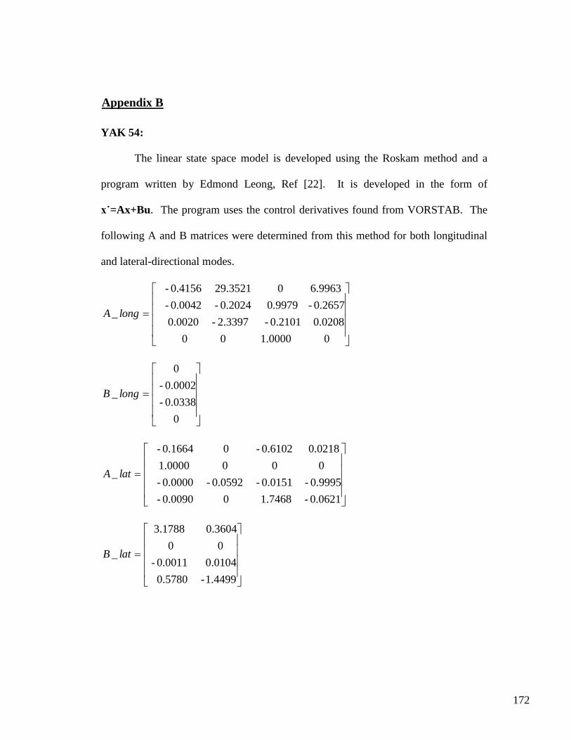
172

Appendix B

YAK 54:

The linear state space model is developed using the Roskam method and a

program written by Edmond Leong, Ref [22]. It is developed in the form of

x˙=Ax+Bu. The program uses the control derivatives found from VORSTAB. The

following A and B matrices were determined from this method for both longitudinal

and lateral-directional modes.

0 1.0000 0 0

0.0208 0.2101- 2.3397- 0.0020

0.2657- 0.9979 0.2024- 0.0042-

6.9963 0 29.3521 0.4156-

_ longA

0

0.0338-

0.0002-

0

_ longB

0.0621- 1.7468 0 0.0090-

0.9995- 0.0151- 0.0592- 0.0000-

0 0 0 1.0000

0.0218 0.6102- 0 0.1664-

_ latA

1.4499- 0.5780

0.0104 0.0011-

0 0

0.3604 3.1788

_ latB

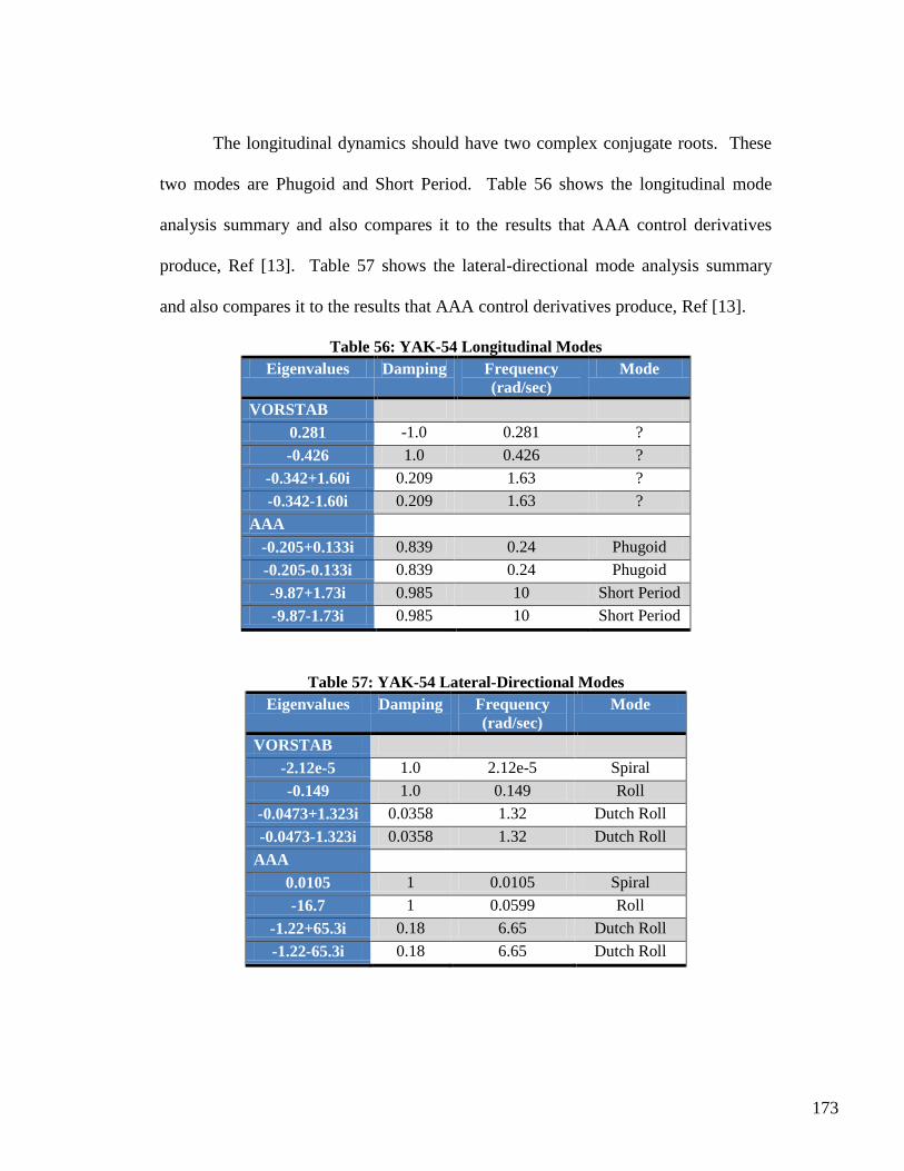
173

The longitudinal dynamics should have two complex conjugate roots. These

two modes are Phugoid and Short Period. Table 56 shows the longitudinal mode

analysis summary and also compares it to the results that AAA control derivatives

produce, Ref [13]. Table 57 shows the lateral-directional mode analysis summary

and also compares it to the results that AAA control derivatives produce, Ref [13].

Table 56: YAK-54 Longitudinal Modes

Eigenvalues Damping Frequency

(rad/sec)

Mode

VORSTAB

0.281 -1.0 0.281 ?

-0.426 1.0 0.426 ?

-0.342+1.60i 0.209 1.63 ?

-0.342-1.60i 0.209 1.63 ?

AAA

-0.205+0.133i 0.839 0.24 Phugoid

-0.205-0.133i 0.839 0.24 Phugoid

-9.87+1.73i 0.985 10 Short Period

-9.87-1.73i 0.985 10 Short Period

Table 57: YAK-54 Lateral-Directional Modes


(rad/sec)

Mode

VORSTAB

-2.12e-5 1.0 2.12e-5 Spiral

-0.149 1.0 0.149 Roll

-0.0473+1.323i 0.0358 1.32 Dutch Roll

-0.0473-1.323i 0.0358 1.32 Dutch Roll

AAA

0.0105 1 0.0105 Spiral

-16.7 1 0.0599 Roll

-1.22+65.3i 0.18 6.65 Dutch Roll

-1.22-65.3i 0.18 6.65 Dutch Roll

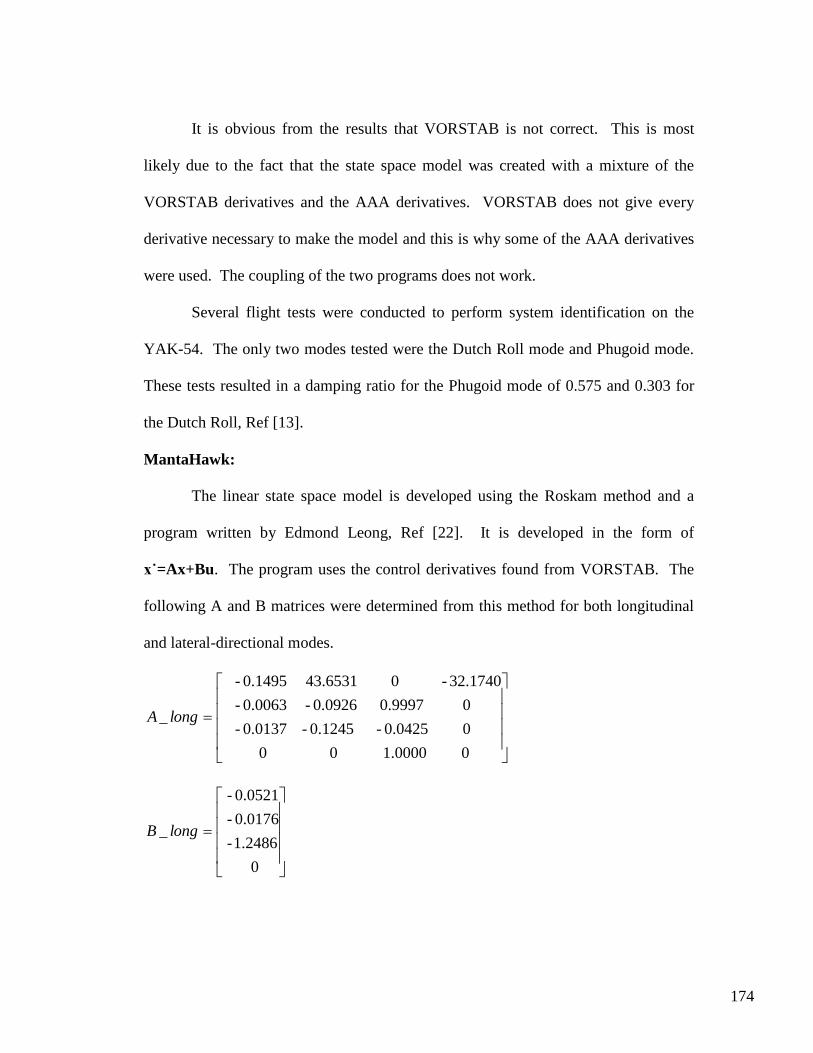
174

It is obvious from the results that VORSTAB is not correct. This is most

likely due to the fact that the state space model was created with a mixture of the

VORSTAB derivatives and the AAA derivatives. VORSTAB does not give every

derivative necessary to make the model and this is why some of the AAA derivatives

were used. The coupling of the two programs does not work.

Several flight tests were conducted to perform system identification on the

YAK-54. The only two modes tested were the Dutch Roll mode and Phugoid mode.

These tests resulted in a damping ratio for the Phugoid mode of 0.575 and 0.303 for

the Dutch Roll, Ref [13].

MantaHawk:





and lateral-directional modes.

0 1.0000 0 0

0 0.0425- 0.1245- 0.0137-

0 0.9997 0.0926- 0.0063-

32.1740- 0 43.6531 0.1495-

_ longA

0

1.2486-

0.0176-

0.0521-

_ longB

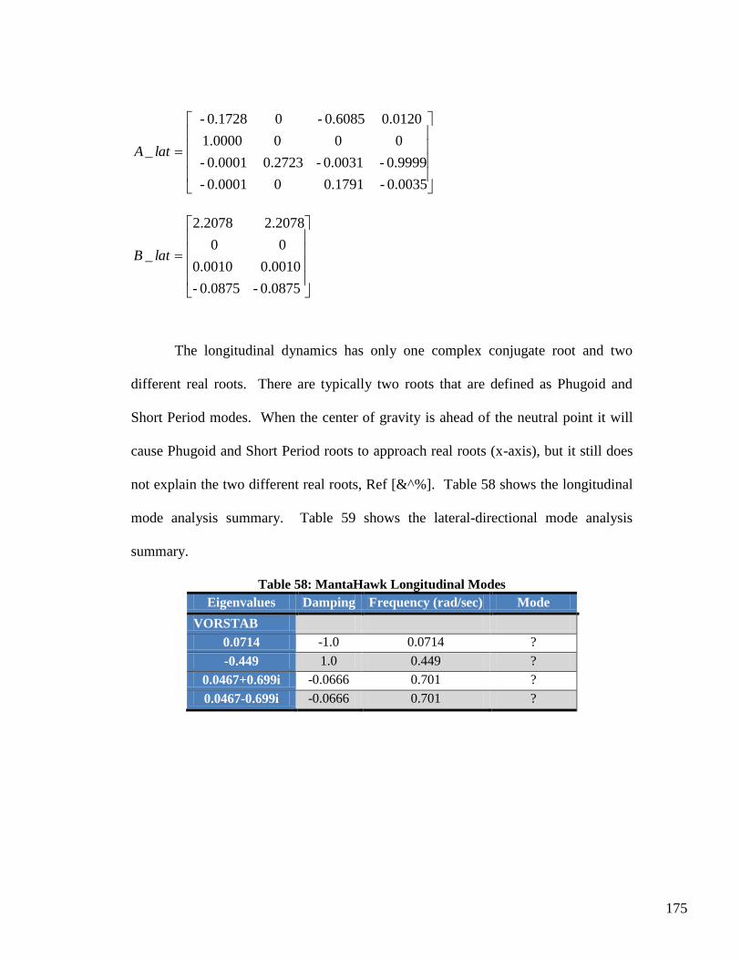
175

0.0035- 0.1791 0 0.0001-

0.9999- 0.0031- 0.2723 0.0001-

0 0 0 1.0000

0.0120 0.6085- 0 0.1728-

_ latA

0.0875- 0.0875-

0.0010 0.0010

0 0

2.2078 2.2078

_ latB

The longitudinal dynamics has only one complex conjugate root and two

different real roots. There are typically two roots that are defined as Phugoid and

Short Period modes. When the center of gravity is ahead of the neutral point it will

cause Phugoid and Short Period roots to approach real roots (x-axis), but it still does

not explain the two different real roots, Ref [&^%]. Table 58 shows the longitudinal

mode analysis summary. Table 59 shows the lateral-directional mode analysis

summary.

Table 58: MantaHawk Longitudinal Modes

Eigenvalues Damping Frequency (rad/sec) Mode

VORSTAB

0.0714 -1.0 0.0714 ?

-0.449 1.0 0.449 ?

0.0467+0.699i -0.0666 0.701 ?

0.0467-0.699i -0.0666 0.701 ?

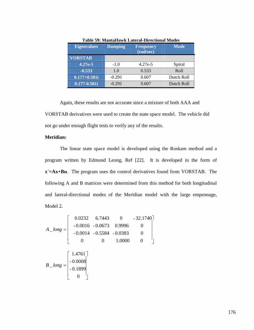
176

Table 59: MantaHawk Lateral-Directional Modes


(rad/sec)

Mode

VORSTAB

4.27e-5 -1.0 4.27e-5 Spiral

-0.533 1.0 0.533 Roll

0.177+0.581i -0.291 0.607 Dutch Roll

0.177-0.581i -0.291 0.607 Dutch Roll

Again, these results are not accurate since a mixture of both AAA and

VORSTAB derivatives were used to create the state space model. The vehicle did

not go under enough flight tests to verify any of the results.

Meridian:





and lateral-directional modes of the Meridian model with the large empennage,

Model 2.

0 1.0000 0 0

0 0.0383- 0.5584- 0.0014-

0 0.9996 0.0673- 0.0016-

32.1740- 0 6.7443 0.0232

_ longA

0

0.1899-

0.0008-

1.4761

_ longB

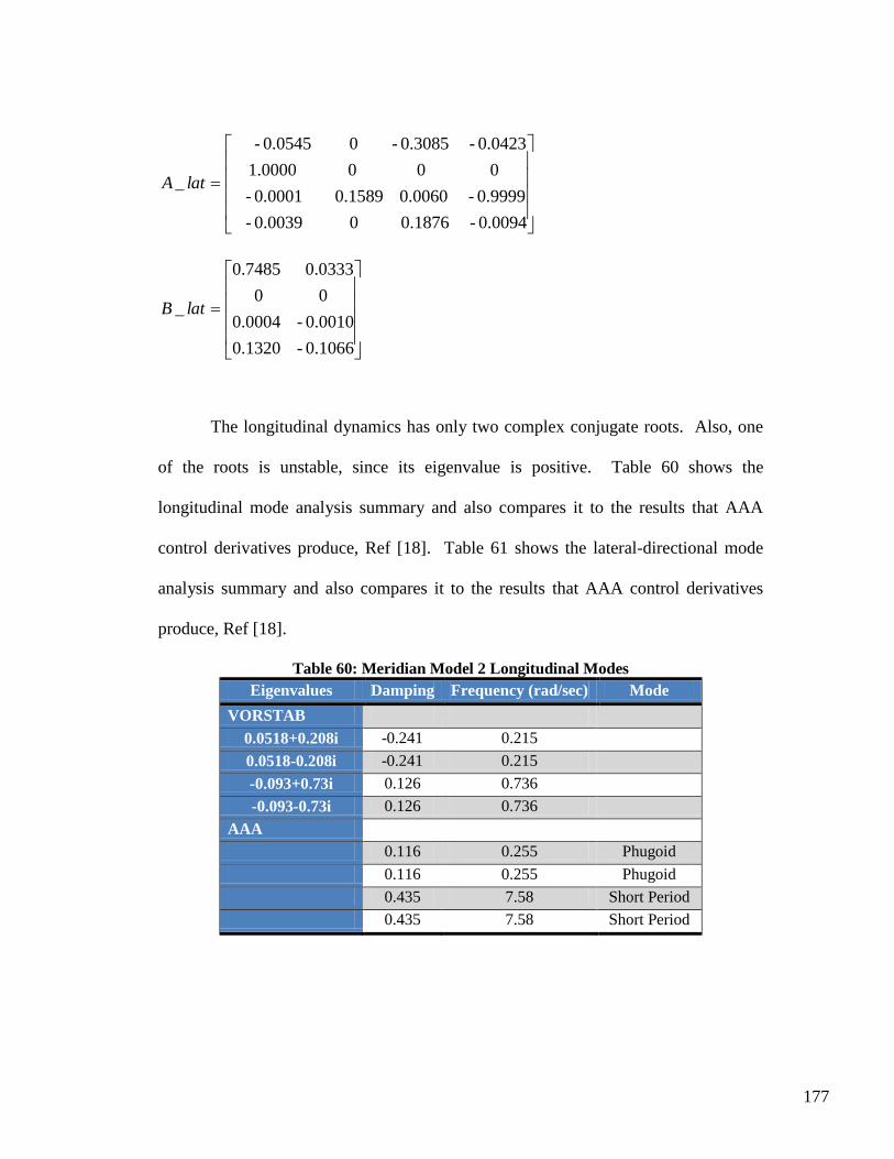
177

0.0094- 0.1876 0 0.0039-

0.9999- 0.0060 0.1589 0.0001-

0 0 0 1.0000

0.0423- 0.3085- 0 0.0545-

_ latA

0.1066- 0.1320

0.0010- 0.0004

0 0

0.0333 0.7485

_ latB

The longitudinal dynamics has only two complex conjugate roots. Also, one

of the roots is unstable, since its eigenvalue is positive. Table 60 shows the

longitudinal mode analysis summary and also compares it to the results that AAA

control derivatives produce, Ref [18]. Table 61 shows the lateral-directional mode

analysis summary and also compares it to the results that AAA control derivatives

produce, Ref [18].

Table 60: Meridian Model 2 Longitudinal Modes


VORSTAB

0.0518+0.208i -0.241 0.215

0.0518-0.208i -0.241 0.215

-0.093+0.73i 0.126 0.736

-0.093-0.73i 0.126 0.736

AAA

0.116 0.255 Phugoid

0.116 0.255 Phugoid

0.435 7.58 Short Period


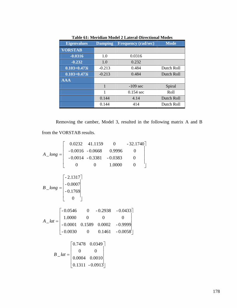
178

Table 61: Meridian Model 2 Lateral-Directional Modes


VORSTAB

-0.0316 1.0 0.0316

-0.232 1.0 0.232

0.103+0.473i -0.213 0.484 Dutch Roll

0.103+0.473i -0.213 0.484 Dutch Roll

AAA

1 -109 sec Spiral

1 0.154 sec Roll

0.144 4.14 Dutch Roll

0.144 414 Dutch Roll

Removing the camber, Model 3, resulted in the following matrix A and B

from the VORSTAB results.

0 1.0000 0 0

0 0.0383- 0.3381- 0.0014-

0 0.9996 0.0668- 0.0016-

32.1740- 0 41.1159 0.0232

_ longA

0

0.1769-

0.0007-

2.1317-

_ longB

0.0058- 0.1461 0 0.0030-

0.9999- 0.0002 0.1589 0.0001-

0 0 0 1.0000

0.0433- 0.2938- 0 0.0546-

_ latA

0.0913- 0.1311

0.0010 0.0004

0 0

0.0349 0.7478

_ latB

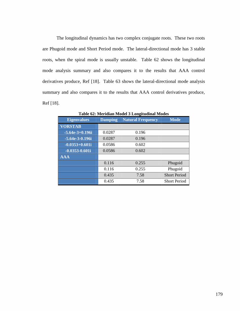
179

The longitudinal dynamics has two complex conjugate roots. These two roots

are Phugoid mode and Short Period mode. The lateral-directional mode has 3 stable

roots, when the spiral mode is usually unstable. Table 62 shows the longitudinal

mode analysis summary and also compares it to the results that AAA control

derivatives produce, Ref [18]. Table 63 shows the lateral-directional mode analysis

summary and also compares it to the results that AAA control derivatives produce,

Ref [18].

Table 62: Meridian Model 3 Longitudinal Modes

Eigenvalues Damping Natural Frequency Mode

VORSTAB

-5.64e-3+0.196i 0.0287 0.196

-5.64e-3-0.196i 0.0287 0.196

-0.0353+0.601i 0.0586 0.602

-0.0353-0.601i 0.0586 0.602

AAA

0.116 0.255 Phugoid

0.116 0.255 Phugoid



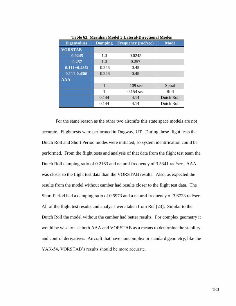
180

Table 63: Meridian Model 3 Lateral-Directional Modes


VORSTAB

-0.0245 1.0 0.0245

-0.257 1.0 0.257

0.111+0.436i -0.246 0.45

0.111-0.436i -0.246 0.45

AAA

1 -109 sec Spiral

1 0.154 sec Roll



For the same reason as the other two aircrafts this state space models are not

accurate. Flight tests were performed in Dugway, UT. During these flight tests the

Dutch Roll and Short Period modes were initiated, so system identification could be

performed. From the flight tests and analysis of that data from the flight test team the

Dutch Roll damping ratio of 0.2163 and natural frequency of 3.5341 rad/sec. AAA

was closer to the flight test data than the VORSTAB results. Also, as expected the

results from the model without camber had results closer to the flight test data. The

Short Period had a damping ratio of 0.5973 and a natural frequency of 3.6723 rad/sec.

All of the flight test results and analysis were taken from Ref [23]. Similar to the

Dutch Roll the model without the camber had better results. For complex geometry it

would be wise to use both AAA and VORSTAB as a means to determine the stability

and control derivatives. Aircraft that have noncomplex or standard geometry, like the

YAK-54, VORSTAB‟s results should be more accurate.

Documents

CFD ANALYSIS OF UAVs USING VORSTAB, FLUENT, AND …