International Inflation Spillovers Through Input Linkages∗

Raphael A. Auer

Bank for International Settlements

Swiss National Bank and CEPR

Andrei A. Levchenko

University of Michigan

NBER and CEPR

Philip Saure

Swiss National Bank

February 3, 2016

Abstract

We examine whether observed international input linkages synchronize inflation across coun-

tries. Using a multi-country, industry-level dataset that combines information on producer

prices and exchange rates with international and domestic input linkages, we recover the cost

shocks underlying the observed changes in PPI in our sample of countries. We then compare

the extent to which common world factors account for the variation in actual PPI compared

to the variation in the underlying cost shocks. Our main finding is that input linkages can

account for one-third to one-half of the global common component of observed producer price

inflation in the data. The contribution of input linkages to synchronization is high when the

pass-through of cost shocks is high, and when exchange rate movements are taken into ac-

count. We report two additional findings: (i) common sectoral shocks are the primary driver

of PPI synchronization across countries, and input linkages amplify comovement primarily by

propagating sectoral shocks across countries; and (ii) the unbalanced nature of international

input use preserves fat-tailed idiosyncratic shocks and thus leads to fat-tailed global inflation,

i.e. periods of disinflation and high inflation.

JEL Classifications: F33, F41, F42

Keywords: international inflation synchronization, input linkages

∗We are grateful to workshop participants at 2015 CEPR ESSIM and the Swiss National Bank for helpfulsuggestions, and to Andreas Kropf, Bogdan Bogdanovic, Julian Ludwig, Pierre Yves Deleamont, Gian Marco Humm,and Barthelemy Bonadio for excellent research assistance. We would especially like to thank Christopher Otrokfor sharing his factor model estimation code with us. The views expressed in this study do not necessarily reflectthose of the institutions with which the authors are affiliated. E-mail: raphael.auer@snb.ch, alev@umich.edu,philip.saure@snb.ch.

1 Introduction

Inflation rates exhibit strong positive cross-country comovement. Understanding the reasons

behind international inflation synchronization is important in a variety of contexts, such as infla-

tion forecasting, optimal monetary policy, international policy coordination, and currency unions,

among others.1 The positive inflation comovement across countries has been attributed to the

increased real integration of the global economy. This paper evaluates the hypothesis that the

observed international inflation comovement is due in part to the cross-border propagation of cost

shocks through input-output linkages.

The following simple expression conveys the main idea. Abstracting from the sectoral dimen-

sion, suppose that country c’s production uses inputs from country s. Then the log change in PPI

of country c can be expressed as

PP Ic = γc,s × β × PP Is + Cc, (1)

where Cc is the change in the local costs in c (which could be due to changes in productivity,

prices of primary factors, or local intermediate inputs). The extent to which s’s inflation shocks

propagate to c is a product of two values: the cost share of inputs from s in the value of output

of c, γc,s, and the cross-border pass-through β that governs how much of the local price change

in s is actually passed on to foreign buyers.

This paper assembles a unique dataset that combines monthly disaggregated producer price

indices (PPIc) with information on sectoral domestic and international input trade from the World

Input Output Database (WIOD). The WIOD provides information on cross-border input shares

γc,s by country pair and sector pair. Our data cover 30 countries and 16 sectors over the period

1995-2012. The baseline analysis assumes full pass-through of cost shocks to input buyers: β = 1.

This allows us to focus more squarely on the properties of the global input-output structure,

and is an appropriate benchmark in this context. Berman, Martin and Mayer (2012) report an

exchange rate pass-through coefficient for intermediate inputs of 0.93, or close to complete, and

much higher than pass-through into the prices of consumer goods. Amiti, Itskhoki and Konings

(2014) find that firms that do not import inputs have a nearly complete pass-through of exchange

rate shocks, suggesting that firms transmit their costs shocks nearly one-to-one into the prices

they charge for their exports.2

We conduct three sets of empirical exercises to gauge the importance of the global supply

chain for producer price inflation. As a preliminary step to document the potential magnitudes of

1See the survey in Corsetti, Dedola and Leduc (2010).2Section 3.3.2 provides a more detailed discussion and presents results under different assumptions on pass-

through.

1

the effects investigated in the paper, we simulate hypothetical inflation shocks and compute how

they propagate through the global IO linkages. On average in the full sample of country pairs, the

elasticity of cross-border propagation of country-specific shocks is low. For the most important

countries, a shock that increases inflation by 1% leads to inflation on the order of 0.015-0.042%

on average in the rest of the country sample. However, this limited transmission hides a great

deal of heterogeneity. The most important countries have a larger impact on its closest trading

partners. For instance, an inflationary shock to Germany transmits with an elasticity of 0.11 to

Hungary, Czech Republic, and Austria. Similar magnitudes characterize other closely integrated

countries, such as US, Canada, and Mexico; or China, Korea, and Taiwan.

It is not surprising that the bilateral impact of an individual country’s inflationary shock on

other countries is limited on average. However, global inflation shocks transmit significantly into

countries. When we generate shocks that raise inflation by 1% in every other country in the world

other than the country under observation, we find that a 1% global PPI inflation shock leads to an

average increase of 0.23% in domestic PPI in our sample of countries. Again, there is substantial

heterogeneity. At the top end there are 5 countries with elasticities with respect to global inflation

over 0.3: Hungary, Belgium, Czech Republic, Slovenia, and Lithuania. Russia, Australia, Japan,

and the US appear the least susceptible to global inflation shocks, with elasticities in the range

of 0.08-0.12.

The second exercise uses a generalization of the relationship (1) and data on the PPI’s and γc,s

to recover the underlying cost shocks Cc under full pass-through of cost shocks. We then compare

the extent of cross-country synchronization in the actual PPI’s with the extent of synchronization

in the underlying cost shocks Cc. The incremental increase in synchronization of actual PPI’s

compared to Cc is then attributed to the cross-border propagation of inflationary shocks through

input linkages.3 Our metrics of international inflation synchronization build on Ciccarelli and

Mojon (2010), and are based on the share of the variance of countries’ inflation that is accounted

for by a single global factor.

The main finding is that international input-output linkages can matter a great deal for in-

flation synchronization when pricing to market by input producers is limited. The share of the

variance in the underlying shocks Cc attributable to the common global factor is one-third to

one-half lower than the global factor’s share of the variance in the actual PPI’s.

To better understand this result, we present several variations on this exercise designed to

isolate the role of domestic and international linkages, pass-through, and global sectoral shocks.

To probe the role of international input linkages, we compute the counterfactual PPI’s that would

obtain under the same underlying cost shocks, but with only domestic input linkages. In addition,

3The approach is akin to Foerster, Sarte and Watson (2011)’s analysis of the role of input linkages in US sectoraloutput comovement.

2

to examine the impact of cross-sectoral and cross-country heterogeneity in input linkages, we re-

implement the model with homogeneous rather than heterogeneous linkages, such that input trade

in each sector and country is equal to the average input trade across all sectors and countries. All

in all, re-introducing domestic input linkages or making the international linkages homogeneous

delivers results similar to the baseline. We conclude that what matters quantitatively is the overall

extent of international linkages, rather than their precise heterogeneous configuration.

Next, we examine the role of imperfect pass-through and exchange rate shocks. We report the

results under the values of β ranging between 0.3 (which is at the lower end of available estimates)

and 1. At the extreme, then β = 0.3, the contribution of input linkages to synchronization is

still positive, but much lower than in the baseline, at 10–15%. This is not surprising. Equation

(1) makes it clear that in the limit as pass-through goes to zero (β → 0), Cc = PP Ic and the

contribution of input linkages to synchronization is trivially nil. As β increases, the importance

of input linkages for inflation synchronization rises monotonically. In addition, we implement an

exercise in which the exchange rate movements are ignored (equivalently, exchange rate changes

are assumed to have the pass-through coefficient β = 0, but PPI shocks remain). In this im-

plementation, the contribution of input linkages is also lower, at 10-20%. Thus, understanding

whether and how input goods are priced to market is central to quantifying the ultimate im-

portance of the international supply chain for producer price comovement. Whenever firms pass

through exchange rate and cost shocks only partially into the prices they charge for their exports,

the transmission of an inflationary shock over subsequent nodes of the production chain is muted,

thus limiting the role of input-output trade for global inflation comovement. Our analysis makes

this point quantitatively precise.

We then implement a dynamic factor model that decomposes the underlying sector-level PPI

fluctuations into the world, global sectoral, and country factors following the methodology devel-

oped in Jackson, Kose, Otrok and Owyang (2015). We assess the contribution of each of those

factors to aggregate PPI synchronization through input linkages. In this model, international

comovement in PPI could be due to a common world factor affecting all PPI series, or to sectoral

factors that are also common across countries. We find that the observed common component of

aggregate PPI is due primarily to the sectoral common components, rather than a single world fac-

tor. Furthermore, input linkages contribute to PPI synchronization primarily through increasing

the relative importance of sectoral rather than world shocks.

The last part of the paper assesses the role of global input linkages in transmitting tail inflation

risks. Using the approach in Acemoglu, Ozdaglar and Tahbaz-Salehi (2015), we show that country-

level inflation rates have fat tails, when measured against a normal benchmark. These fat tails in

actual inflation are inherited from the underlying cost shocks, which are themselves significantly

more fat-tailed than a normal distribution. Comparing the distributions of actual PPI and the

3

underlying cost shocks, it appears that the IO matrix itself neither accentuates nor dampens the

underlying tail risks, as the PPI is about as fat-tailed as the cost shocks. However, this finding is

itself evidence that the structure of input linkages is such that the fat-tailed shocks are preserved.

Acemoglu et al. (2015) show that a more “balanced” IO matrix would average out fat-tailed

shocks and lead inflation outcomes well-approximated by a normal distribution.

Our analysis contributes to the literature on cross-border inflation synchronization and its de-

terminants. Monacelli and Sala (2009), Burstein and Jaimovich (2012), Andrade and Zachariadis

(2014), and Beck, Hubrich and Marcellino (2015) study the comovement of international prices us-

ing micro data, while Ciccarelli and Mojon (2010), Mumtaz and Surico (2009, 2012) and Mumtaz,

Simonelli and Surico (2011) examine the role of aggregate real linkages in inflation comovement.

Borio and Filardo (2007) and Bianchi and Civelli (2015) address the related question of how much

global output gaps affect domestic inflation dynamics. Bems and Johnson (2012, 2015) and Patel,

Wang and Wei (2014) combine data on global input linkages with domestic prices and exchange

rates to construct theoretically-founded measures of real exchange rates. Our paper is the first

to use information on observed international input linkages to evaluate the hypothesis that these

linkages synchronize PPI inflation across countries.

While understanding the mechanisms underlying global inflation synchronization is important

in its own right, our results can also help shed light on the role of input linkages in business cycle

synchronization more broadly. Up until now, the literature on input linkages and international

comovement has focused exclusively on comovement in quantities or volumes (Kose and Yi 2006,

Burstein, Kurz and Tesar 2008, di Giovanni and Levchenko 2010, Johnson 2014). While the

quantity approach has more direct implications for the comovement in real GDP, the question

of whether quantities comove across countries hinges on the elasticity of substitution between

imported inputs and domestic value added. This elasticity is a parameter about which little or

nothing was known empirically until very recently (see the recent work by Boehm, Flaaen and

Pandalai-Nayar 2014, for an estimate). The advantage of using prices instead of quantities is that

(for small changes), the impact on prices does not depend on the elasticity of substitution whereas

the response of quantities does.

The rest of the paper is organized as follows. Section 2 presents the data and the estimation

procedure. Section 3 describes the main results on inflation synchronization, and Section 4 on the

role of input linkages in propagating inflation tail risks. Section 5 concludes.

4

2 Data Description and Implementation

2.1 Data

To carry out the analysis requires data on (i) industry-level PPI and (ii) cross-border input-

output linkages. A contribution of our paper is the construction of a cross-country panel dataset

of monthly sectoral producer prices that can be merged with existing datasets on input-output

use.

The PPI data were collected from international and national sources. The frequency is

monthly. The PPI series come from the Eurostat database for those countries covered by it.

Because many important countries (US, Canada, Japan, China) are not in Eurostat, we collected

PPI data for these countries from national sources, such as the BLS for the US and StatCan for

Canada. Unfortunately, the sectoral classifications outside of Eurostat tend to be country-specific,

and require manual harmonization.

Information on input linkages comes the World Input-Output database (WIOD) described in

Timmer, Dietzenbacher, Los, Stehrer and de Vries (2015), that provides a global input-output

matrix. It reports, for each country and output sector, input usage broken down by source sector

and country. The WIOD is available at yearly frequency, and covers about 40 countries. Merging

the PPI and WIOD databases required further harmonization of the country and sector coverage.

The sectoral classification of the original PPI series are concorded to the classification that can

be merged with the WIOD database, which uses two-letter categories that correspond to the

ISIC (rev. 2) sectoral classification. Appendix Table A1 shows the conversion tables used in the

process.

The final sample includes 30 countries plus a composite Rest of the World (ROW) category,

16 tradeable sectors, and runs from 1995m1 to 2011m12. Appendix Table A2 reports the list of

countries and sectors used in the analysis. Additionally, some countries are included in the “rest

of the world” category because of a too large share (> 0.4) of missing data in the PPI. These are

summarized in Appendix Table A3.

The empirical methodology requires a balanced sample of countries×sectors×months, necessi-

tating some interpolation. When the original PPI frequency is quarterly, the monthly PPI levels

are interpolated from the quarterly information. Other missing PPI observations are extrapolated

using a regression of a series inflation on seasonal monthly dummies (e.g. a missing observation for

January is set to the average January inflation for that series). If a country-sector series is missing

over the entire time horizon (19 cases out of the 496 series), its inflation values are extrapolated

based on the rest of the country’s series. Overall, 12.7% of the PPI values are extrapolated.

An important feature of the PPI index is that it only covers the industrial sector in the

majority of countries. Thus, service sector prices are not included in the analysis.

5

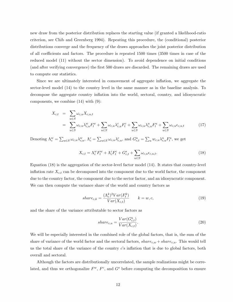
Figure 1 reports the share of foreign inputs in the overall input usage in each country. On

average in this sample of countries, 0.4 of the total input usage comes from foreign inputs, but

there is a great deal of variation, from less than 0.2 for Russia, China, and Japan to nearly 0.8

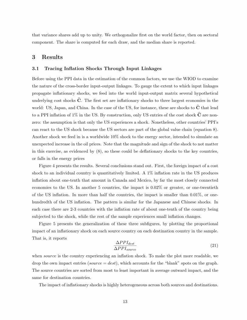
for Belgium. Figure 2 reports the cross-sectoral variation in the same measure, defined as the

share of imported inputs in the total input usage in a particular sector worldwide. Sectors differ

in their input intensity, with 0.4 of all inputs being imported in the Coke and Petroleum sector,

but only 0.1 in the Food and Beverages sector.

Figure 3 gives a sense of the time variation in the intensity of foreign input usage. The share

of foreign inputs in total input purchases rose from about 0.2 to over 0.3 from 1995 to the eve of

the Great Trade Collapse, and then fell to 0.25.

2.2 Implementation

There are C countries indexed by c and e, and S sectors indexed by u and s. The world is

characterized by global input linkages: sector u producing output in country c has a cost function

Wc,u,t = W (Cc,u,t,pc,u,t), (2)

where pc,u,t ≡ {pc,u,e,s,t}s=1,...Se=1,...,C is the vector of prices of inputs from all the possible source

countries s and sectors e paid by sector u in country c. Input prices pc,u,e,s,t are indexed by

the purchasing country-sector to reflect the fact that prices actually paid by each sector in each

country for the same input may differ. The cost of value added is denoted by Cc,u,t. This cost

embodies the wage bill and the cost of capital.4

Standard steps using Shephard’s Lemma and Euler’s Theorem yield the following approxima-

tion for the change in the cost function:

Wc,u,t ≈ γCc,u,t−1Cc,u,t +∑e,s

γIc,u,e,s,t−1pc,u,e,s,t, (3)

where the hat denotes proportional change (xt = xt/xt−1 − 1). In this expression, γCc,u,t−1 is the

share of value added in the value of total output, and γIc,u,e,s,t is the share of expenditure on input

e,s by sector-country c,u in the value of total output of sector c,u at time t. Notice that the shares

γIc,u,e,s,t depend on prices and may thus correlate with prices. Therefore, these shares are lagged

by one year in expression (3).

To apply this expression to the data, we make two assumptions. First, the proportional

change in the producer price index as measured in the data is the same as the change in the

4In the exposition that follows, as a shorthand we refer to Cc,u,t as the cost of value added. Since the PPI dataused in the empirical implementation only cover industrial sectors, in the analysis below Cc,u,t actually includesthe cost of any inputs that are not in the set of sectors that comprise the PPI (such as service sector inputs).

6

cost function: PP Ic,u,t = Wc,u,t. Two settings in which this holds are marginal cost pricing and

constant markups over marginal cost. This assumption is violated when markups are variable. In

that case, our procedure will attribute the change in the markup to a change in the cost of value

added γCc,u,t−1Cc,u,t.

Second, the change in the price paid by producers in c,u for inputs from e,s is given by:

pc,u,e,s,t = βIc,u,e,s

(We,s,t + Ec,e,t

), (4)

where Ec,e,t is the change in the exchange rate between c and e. That is, the changes in prices

paid by c,e for inputs are proportional to the change in the cost function of the input-supplying

sector We,s,t and the change in the exchange rate. The proportionality constant βIc,u,e,s can be

less than 1, to account for imperfect pass-through of cost and exchange rate shocks to prices.

The cost shock Cc,u,t for each country c and sector u is then recovered directly, based on

equations (3) and (4):

Cc,u,t =1

γCc,u,t−1

PP Ic,u,t − ∑e∈C,s∈S

βIc,u,e,sγIc,u,e,s,t−1

(PP Ie,s,t + Ec,e,t

) , (5)

In this expression, all the PP Ic,u,t’s, Ec,e,t’s, γIc,u,e,s,t−1, and γCc,u,t−1 are taken directly from the

data.

It will be convenient to express (5) in matrix notation:

C = D−1[(I−B′ ◦ Γ′)PPI− B′ ◦ Γ

′E]. (6)

In this expression, C and PPI are the CS×1 vectors of all country-sector cost shocks and PPI’s.

The matrix Γ is the CS × CS global input-output matrix whose ij’th element is the share of

spending on input i in total value of sector j’s output, where i and j index country-sectors. B′

is the CS × CS matrix that collects the βIc,u,e,s coefficients, and “◦” denotes element-by-element

multiplication. Finally, D is a CS × CS diagonal matrix whose diagonal entries are the γCc,u,t−1

coefficients.

In the last term,

E =

E1,t

...

EC,t

⊗ 1S×1

where Ec,t an C × 1 vector of exchange rate changes experienced by country c relative to its

trading partners, and thus E is the CC × 1 vector of stacked exchange rate changes that only

7

vary by country. The matrix Γ′

is:

Γ′=

Γ′1 0 . . . 0

0 Γ′2 0 . . .

0 0 . . . 0

0 . . . 0 Γ′C

, (7)

with Γ′c defined as the S × CS matrix whose rows are country c’s rows of Γ′, and B′ is defined

analogously based on B′.

To streamline notation, the time subscripts are suppressed in the matrix notation.

2.3 Simulating the International Inflation Comovement Using Input-Output

Data

To simulate the impact of hypothetical shocks, we make use of the relation (6) to go from the

shocks to the resulting PPI. This requires solving for the equilibrium PPI’s using the Leontief

inverse. Stacking countries and sectors, assuming full-pass-through (βIc,u,e,s = 1), and ignoring

exchange rate movements, the equilibrium PPI’s given a vector of cost shocks are:

PPI =(I− Γ′

)−1DC. (8)

2.4 Recovering Underlying Cost Shocks and Estimating Comovement in the

Data

Equation (5) is used together with monthly frequency PPI data to recover the underlying cost

shocks Cc,u,t for every country, sector, and month. Equation (5) does not involve any lags,

amounting to the assumption that imported inputs are shipped and used within the month.

Monthly data feature seasonality that potentially differs by country and sector, and correcting

explicitly for such seasonality is not feasible in our data. Thus, we follow the common practice of

transforming both the actual PPI data and the underlying cost shock data into 12-month changes:

PP I12c,u,t =11∏τ=0

(1 + PP Ic,u,t−τ )− 1

and

C12c,u,t =11∏τ=0

(1 + Cc,u,t−τ )− 1.

The ultimate object of interest is the country-level rather than sector-level inflation. With

8

that objective, we aggregate sectoral PPI’s and cost shocks using sectoral output weights:

PP I12c,t =∑u∈S

ωc,uPP I12c,u,t (9)

and

C12c,t =∑u∈S

ωc,uC12c,u,t, (10)

where ωc,u is the share of sector u in total output of country c. We pick the 2002 sectoral output

weights, the year close to the middle of the sample.

The object in (9) has a clear interpretation: it is the aggregate PPI of country c. The aggregate

PPI series we build track closely (though not perfectly) the official aggregate PPI’s in our sample

of countries.5The object in (10) is the output-share weighted composite cost shock in country c.

It can be interpreted as the PPI in country c in the counterfactual world without input linkages in

production. For maximum consistency between the two measures, the construction of C12c,t uses

the same sectoral weights ωc,u as that of PP I12c,t. This ignores the possibility that had there

been no input linkages, output shares would be different. Without a full-fledged model calibrated

with all the relevant elasticities, it would be impractical to specify a set of counterfactual output

shares. Our approach has the virtue of transparency and maximum comparability between the

actual PPI’s and the counterfactual cost measures.

We employ three metrics for the extent of international synchronization in PP I12c,t and

C12c,t. It is important to emphasize that these are simply statistical devices that summarize the

extent of the comovement in a data sample. The first, following Ciccarelli and Mojon (2010),

is the R2 of the regression of each country’s PP I12c,t and C12c,t on the corresponding global

average of the same measure (excluding the country itself).

The second and third are based on estimating a factor model on the panel of PPI and cost

shock series:

Xc,t = λcFt + εc,t, (11)

where the left-hand variable Xc,t is, alternatively, PP I12c,t or C12c,t. According to (11), the

cross-section of inflation rates/cost shocks at any t is equal to a factor Ft common to all countries

times a country-specific, non-time varying coefficient λc, plus a country-specific idiosyncratic

shock εc,t. None of the objects in the right-hand side of (11) are observed, but can be estimated.

As is customary, the factor analysis is implemented after standardizing each country’s data to

have mean zero and standard deviation of 1. This ensures that countries with more volatile

5In our sample of countries, the mean correlation between our constructed aggregate PPI and the official PPI,in 12 month changes, is 0.67, and the median is 0.75. The minimum is 0.01 for Bulgaria, which experiencedhyperinflation between 1995 and 1998 (after 1998, the correlation for Bulgaria is 0.75). The maximum is 0.97(Japan).

9

inflation rates do not have a disproportionate impact on the estimation of the common factor.

After estimating the factor model, the metric for synchronization is the share of the variance of

inflation in country c accounted for by the global factor Ft: V ar(λcFt)/V ar(Xc,t).

We implement two variations of (11). The first is a static factor model in which the parameters

are recovered through principal components, as in Ciccarelli and Mojon (2010). The second is a

dynamic factor model based on Jackson et al. (2015) in which both Ft and εc,t are assumed to

follow AR(p) processes:

Ft =∑

l=1..pF

φlFt−l + ut (12)

εc,t =∑l=1..pε

ρc,lεc,t−l + µc,t. (13)

The precise implementation of the Bayesian estimation of this model’s parameters is a reduced,

special case of the more general one described in the following subsection.

2.5 The Sectoral Dimension

Up to here, we have used different approaches to evaluate the importance of a common world

component from the panel of aggregated country series in the model (11). Our underlying data,

however, are disaggregated at the country-sector level. Examining sector-level data can tell us

more about the nature of the common world factor found above. In particular, by implementing

a sector-level decomposition, we can reveal how much of the common world component is in fact

due to global sectoral shocks, and how a country’s sectoral composition affects its comovement

with the world factor.

To that aim, we use the dynamic factor model developed in Jackson et al. (2015), that is

implemented directly on sector-level data and generalizes the model (11) - (13). Specifically, we

estimate the following model:

Xc,u,t = αc,u + λwc,uFwt + λcc,uF

ct + λuc,uF

ut + εc,u,t (14)

where Xc,u,t is the 12-month inflation rate in country c, sector u, which can be either actual

PP I12c,u,t, the recovered cost shock C12c,u,t, or one of the other counterfactual price series. It

is assumed to comprise of a world factor Fwt common to all countries and sectors in the sample,

the country factor F ct common to all u in country c, a sectoral factor F ut common to all sector u

prices worldwide, and an idiosyncratic error term. Each of these factor series and the error term,

10

in turn, are assumed to follow an AR process, parallel to (12):

F kt =∑

l=1..pF

φk,lFkt−l + uk,t, k = w, c, u (15)

and

εc,u,t =∑l=1..pε

ρc,u,lεc,u,t−l + µc,u,t. (16)

Under the assumptions that uk,t ∼ N(0, 1) for k = w, c, u, and the restriction that the sign of the

loading of the first series on the world factor be positive, the decomposition is well-defined. The

residuals µcs,t are assumed to be distributed

µc,u,t ∼ N(0, σ2c,u).

We follow the Bayesian estimation procedure from Jackson et al. (2015), briefly summarized

here. First, we denote the parameter vector by ξc,u = [ αc,u λc,u ρc,u ], where the vector αc,u

collects the constant terms, λc,u summarizes all loadings and ρc,u = (ρc,u,1, ..., ρc,u,pε) all the AR

coefficients of the errors. The priors of these model parameters are set to

ξc,u ∼ N(0, B−1c,u)

where B−1c,u = diag([.001 ∗ 11+nfactors ,1pε ]), and 1n the n-dimensional vector with the elements

1. Thus, the constants, the loadings, and the error AR coefficients have a prior mean of 0, the

constant and loading a prior variance of 0.001 and the error AR coefficients a prior variance of 1.

Next, the remaining model parameters φk = (φk,1, ..., φk,pF ) have the priors

φk ∼ N(0, Φ−1k ), k = w, c, u

where Φ−1k = diag ( 1 10.85

... 10.85pF ). The prior variance is thus exponentially decreasing with the

lag length, reflecting that further lags have a smaller probability of having a non-zero effect.

Moreover, the variance of µc,u,t, σ2c,u, have the priors

σ2c,u ∼ IG(vc,u/2, δc,u/2),

where IG is the inverted gamma distribution, vc,u = 6, and δc,u = 0.001. Finally, we set pF = 3

and pε = 2. The starting values are 0 for all coefficients and random standard normal draws for

the factors.

The algorithm then computes (implicitly determines) the posterior distribution of each of the

parameters conditional on all other parameters, in the order ξc,u, σ2c,u, φk, and F kt . At each step, a

11

new draw from the posterior distribution replaces the starting value (if granted a likelihood-ratio

criterion, see Chib and Greenberg 1994). Repeating this procedure, the (conditional) posterior

distributions converge and the frequency of the draws approaches the joint posterior distribution

of all coefficients and factors. The procedure is repeated 1500 times (3500 times in case of the

reduced model (11) without the sector dimension). To avoid dependence on initial conditions

(and after verifying convergence) the first 500 draws are discarded. The remaining draws are used

to compute our statistics.

Since we are ultimately interested in comovement of aggregate inflation, we aggregate the

sector-level model (14) to the country level in the same manner as in the baseline analysis. To

decompose the aggregate country inflation into the world, sectoral, country, and idiosyncratic

components, we combine (14) with (9):

Xc,t =∑u∈S

ωc,uXc,u,t

=∑u∈S

ωc,uλwc,uF

wt +

∑u∈S

ωc,uλcc,uF

ct +

∑u∈S

ωc,uλuc,uF

ut +

∑u∈S

ωc,uεc,u,t (17)

Denoting Λwc =∑

u∈S ωc,uλwc,u, Λcc =

∑u∈S ωc,uλ

cc,u, and Guc,t =

∑uwc,uλ

uc,uF

ut , we get

Xc,t = Λwc Fwt + ΛccF

ct +Gsc,t +

∑u∈S

ωc,uεc,u,t. (18)

Equation (18) is the aggregation of the sector-level factor model (14). It states that country-level

inflation rate Xc,t can be decomposed into the component due to the world factor, the component

due to the country factor, the component due to the sector factor, and an idiosyncratic component.

We can then compute the variance share of the world and country factors as

sharec,k =(Λkc )

2V ar(F kt )

V ar(Xc,t)k = w, c, (19)

and the share of the variance attributable to sector factors as

sharec,u =V ar(Guc,t)

V ar(Xc,t). (20)

We will be especially interested in the combined role of the global factors, that is, the sum of the

share of variance of the world factor and the sectoral factors, sharec,w + sharec,u. This would tell

us the total share of the variance of the country c’s inflation that is due to global factors, both

overall and sectoral.

Although the factors are distributionally uncorrelated, the sample realizations might be corre-

lated, and thus we orthogonalize Fw, F c, and Gs before computing the decomposition to ensure

12

that variance shares add up to unity. We orthogonalize first on the world factor, then on sectoral

component. The share is computed for each draw, and the median share is reported.

3 Results

3.1 Tracing Inflation Shocks Through Input Linkages

Before using the PPI data in the estimation of the common factors, we use the WIOD to examine

the nature of the cross-border input-output linkages. To gauge the extent to which input linkages

propagate inflationary shocks, we feed into the world input-output matrix several hypothetical

underlying cost shocks C. The first set are inflationary shocks to three largest economies in the

world: US, Japan, and China. In the case of the US, for instance, these are shocks to C that lead

to a PPI inflation of 1% in the US. By construction, only US entries of the cost shock C are non-

zero: the assumption is that only the US experiences a shock. Nonetheless, other countries’ PPI’s

can react to the US shock because the US sectors are part of the global value chain (equation 8).

Another shock we feed in is a worldwide 10% shock to the energy sector, intended to simulate an

unexpected increase in the oil prices. Note that the magnitude and sign of the shock to not matter

in this exercise, as evidenced by (8), so these could be deflationary shocks to the key countries,

or falls in the energy prices

Figure 4 presents the results. Several conclusions stand out. First, the foreign impact of a cost

shock to an individual country is quantitatively limited. A 1% inflation rate in the US produces

inflation about one-tenth that amount in Canada and Mexico, by far the most closely connected

economies to the US. In another 5 countries, the impact is 0.02% or greater, or one-twentieth

of the US inflation. In more than half the countries, the impact is smaller than 0.01%, or one-

hundredth of the US inflation. The pattern is similar for the Japanese and Chinese shocks. In

each case there are 2-3 countries with the inflation rate of about one-tenth of the country being

subjected to the shock, while the rest of the sample experiences small inflation changes.

Figure 5 presents the generalization of these three subfigures, by plotting the proportional

impact of an inflationary shock on each source country on each destination country in the sample.

That is, it reports∆PPIdest

∆PPIsource(21)

when source is the country experiencing an inflation shock. To make the plot more readable, we

drop the own impact entries (source = dest), which accounts for the “blank” spots on the graph.

The source countries are sorted from most to least important in average outward impact, and the

same for destination countries.

The impact of inflationary shocks is highly heterogeneous across both sources and destinations.

13

Inflationary shocks to some countries, like Lithuania, Greece, Slovenia, or Bulgaria, have virtually

no discernible impact on inflation in other countries. This is due to those countries not being

important input suppliers to others. At the other end of the spectrum, the top 5 countries in

terms of their impact on foreign inflation are Germany, China, Russia, US, and Italy. Germany’s

impact is both highest on average (0.04 of ∆PPIdest/∆PPIDEU when averaging over dest) across

the whole sample, and the most diffuse. For 10 countries (all of which are in Europe), the impact

is above 0.05, and for the top 3 – Hungary, Czech Republic, and Austria – the impact is above 0.1.

Russia’s impact is about half of Germany’s (0.022), and more concentrated, with only 2 countries

– Lithuania and Bulgaria – with an impact of over 0.05.

It is not surprising that the bilateral impact of an inflationary shock is limited. A related

question is whether global inflation shocks transmit significantly into countries. We thus consider

an experiment in which, for each country, we generate a shock that raises inflation by 1% in every

other country in the world. Figure 6 reports the results. Global inflationary shocks can have

substantial impact on country inflation. On average, a 1% shock to global PPI inflation leads to

a 0.23% increase in domestic PPI. There is substantial heterogeneity, and at the top end there

are 5 countries exhibit elasticities with respect to global inflation over 0.3: Hungary, Belgium,

Czech Republic, Slovenia, and Lithuania. Russia, Australia, Japan, and the US appear the least

susceptible to global inflation shocks, with impacts in the range of 0.08-0.12.

The last panel of Figure 4 reports the global impact of a 10% global energy sector shock.

Not surprisingly since the shock is global, the impact is much stronger and much more spread

out. Nonetheless, it is also remarkable how much heterogeneity there is, from a 3.5% impact in

Lithuania and Russia to 0.2% in Ireland and Slovenia.

3.2 Input Linkages and Global Inflation Comovement

This section reports the main inflation synchronization results. In order to do so, we need to take

a stand on the degree the of pass-through of the price and exchange rate shocks into producer

prices. We present the baseline results under full pass-through of cost shocks: βIc,u,e,s = 1. Berman

et al. (2012) find an exchange rate pass-through coefficient of 0.93, or close to complete, and much

higher than pass-through into the prices of consumer goods. Amiti et al. (2014) find that firms

that do not import inputs have nearly complete pass-through of exchange rate shocks, suggesting

that firms pass their costs shocks nearly one-to-one into the prices they charge for their exports.

Table 1 reports the main results. The panel A reports the R2 metric, Panel B the static factor

model metric, and Panel C the dynamic factor model metric.

The columns labeled PP I12c,t present the results for the actual PPI. We confirm that there

is a great deal of global synchronization in PPI, just as was found for CPI in previous work.

14

The simple average of other countries’ inflation produces an average R2 of 0.38 in this sample

of countries. The global static factor accounts for 0.43 of the variance of the average country’s

inflation at the mean and 0.48 at the median. The dynamic factor delivers very similar averages.

The three methods thus deliver quite similar levels of synchronization in actual PPI. They also

produce similar answers regarding the cross-country variation. In the cross-section of countries,

the R2 metric has a 0.97 correlation with both the static and the dynamic variance shares. The

static and dynamic variance shares have an over 0.99 correlation across countries. According to

all three measures, there is a fair bit of country heterogeneity around these averages, with Spain,

Germany, and Italy being the most synchronized countries according to both metrics, and Mexico,

Romania, and Russia at the other extreme.

The columns labeled C12c,t present the same statistics for the cost shocks, and the columns

labeled “Difference” report the simple difference between the metrics for PPI and the cost shocks.

It is clear that input linkages have a great deal of potential to explain observed synchronization

in PPI. The average R2 for the cost shocks falls to 0.22 (mean) and 0.14 (median). The static

global factor explains 0.31 (mean) and 0.29 (median) of the variation in C12c,t for the average

country, and the dynamic factor 0.28 (mean) and 0.25 (median).

The difference between synchronization metrics for C12c,t and PP I12c,t can be interpreted as

the contribution of global input linkages to the observed inflation synchronization. According to

the most modest metric – the static factor – input linkages account for 29% (42%) of observed

synchronization at the mean (median). The R2 metric implies the largest contribution, with

input linkages responsible for 43% (64%) of observed synchronization at the mean (median). The

dynamic factor results lie in between.

3.3 Understanding the Mechanisms

We now perform a battery of alternative experiments designed to better understand the mecha-

nisms behind the results. Namely, we examine the nature of domestic and international linkages;

the role of exchange rates; the importance of incomplete pass-through; and the relative roles of

world and sectoral shocks.

3.3.1 Domestic and International Linkages

As emphasized above, the baseline analysis simply aggregates the cost shocks, and thus cleans

out the effect of not only international, but also domestic input linkages. There is no obvious

reason why purely domestic linkages should synchronize inflation internationally. Nonetheless, we

construct an alternative counterfactual to be compared to PP I12c,t, that assumes away interna-

tional input linkages but preserves the domestic ones. This exercise constructs counterfactual PPI

15

changes that would obtain under recovered cost shocks C12c,u,t in an economy in which there is

input usage, but all of it domestic. Namely, we define the “autarky” counterfactual PPI change

as:

PPIAUT =(I− Γ′AUT

)−1DC, (22)

where Γ′AUT is the counterfactual input-output matrix that forces all linkages to be domestic:

Γ′AUT =

Γ′AUT,1 0 . . . 0

0 Γ′AUT,2 0 . . .

0 0 . . . 0

0 . . . 0 Γ′AUT,C

, (23)

and the elements of the S × S matrix ΓAUT,c are defined as:

γc,u,s,t =

C∑k=1

γc,u,k,s,t. (24)

That is, in each country c, sector u, all of the input usage observed in the global input-output

matrix is reassigned to be supplied domestically.

The results are reported in Table 2. To facilitate comparison across counterfactuals, the table

reproduces the mean and median of the R2s and of the shares of variance accounted for the static

and dynamic factors for actual PPI and the baseline recovered cost shocks from Table 1. The panel

labeled “Autarky” reports the means and medians for the autarky scenario. These are close to the

baseline C12c,t, indicating that allowing for domestic linkages does not quantitatively change the

main conclusion about the importance of international linkages for international synchronization.

Next, we evaluate the role of heterogeneity in input usage across countries and sectors in

generating these results. To this end, we construct two counterfactual scenarios for PPI under

“balanced” input-output linkages. The first scenario preserves the cross-country heterogeneity in

input usage, but assumes that within each source country, each input-using country has the same

input shares in all the sectors. That is, we assume a counterfactual input-output matrix Γ′b1c,u,e,s

where:

γb1c,u,e,s =1

S2

∑k∈U,l∈U

γc,k,e,l. (25)

That is, for any pair of countries c and e, there is an S × S matrix of input usage that gives

how much of country e’s inputs by sector are used in country c output in each sector. This

counterfactual, labeled “b1”, suppresses heterogeneity across input and output sectors by country-

pair. It is designed to mimic a one-sector model, in which countries use each other’s aggregate

inputs to produce a single output.

16

The second counterfactual instead focuses on cross-country heterogeneity. It implements a

counterfactual scenario in which the input-output matrix is assumed to be Γ′b2c,u,e,s, with

γb2c,u,e,s =

1m2

∑k∈U,l∈U

γc,k,e,l,t if c = e

1(n−1)m2

∑k∈U,l∈U,e′∈C\{c}

γc,k,e′,l,t if c 6= e(26)

That is, is assumes that all domestic linkages are equal to the average domestic linkage observed in

the data, and that all international linkages for all sectors and countries are equal to the average

international linkage. Finally, these counterfactual γ’s are rescaled such that the total share of

value added in output in each sector and country γCc,u remains the same as in the baseline, in

order not to confound the heterogeneity in input linkages per se with overall input intensity.

The counterfactual PPI is given by

PPIcounter =(I− Γ′counter

)−1 (DC + Γ

′counterE

), (27)

for counter = {b1, b2}, where Γcounter is the counterfactual version of (7), that uses the elements

of counterfactual Γ matrix instead of the actual values. Equation (27) suppresses B and B as in

the baseline analysis all the β’s are assumed to be 1.

The panels “Balanced 1” and “Balanced 2” of Table 2 report the results. The shares of

variances accounted for by the common factors are slightly lower than for the actual PPI in this

case, but these values are much closer to the actual PPI than to the baseline cost shocks. This

suggests that average linkages per se is what is most important. Nonetheless, there appears to

be some role for the unbalanced nature of the input linkages: under the Balanced 1 scenario the

share of variance due to the common component is indeed lower than for actual PPI, suggesting

that sectoral heterogeneity does matter somewhat. All in all, the Balanced 1 shares of variance

are 10-20% lower than actual PPI’s shares of variance.

3.3.2 Exchange Rates vs. Price Spillovers, and Various Degrees of Pass-Through

The baseline analysis sets β = 1, i.e., we assume that producers fully pass on cost shocks to their

consumers. A value of β close to 1 is consistent with some recent micro estimates of exchange

rate pass-through at the border. Berman et al. (2012) find that the pass-through into prices

of intermediate inputs is close to complete (0.93) and considerably higher than the one into

prices of consumer goods. Similarly, Amiti et al. (2014) document that for non-importing Belgian

firms, exchange rate pass-through into export prices is close to 1, again suggesting that exporters

transmit their cost shocks almost fully to buyers.

Nonetheless, we acknowledge that for the purposes of the exercise in this paper it is difficult to

17

assign a value to β with a high degree of confidence, for three reasons. First, there is considerable

uncertainty as to what is the relevant exchange rate pass-through coefficient. One major pattern

that has emerged in the literature is that pass-through is much higher when examining the response

of import price indices than when examining the response of individual prices. For example,

Goldberg and Campa (2010) report an estimate of the exchange rate pass-through rate into

import prices of 0.61 in a sample of 19 advanced economies, and Burstein and Gopinath (2015)

report an updated estimate of 0.69. However, pass-through into import prices is estimated to

be much lower when looking at individual import prices. For example, Burstein and Gopinath

(2015) report an average pass-through rate of 0.28 in the large microeconomic dataset underlying

the official US import price indices.6

The discrepancy between pass-through for individual goods and for aggregate series relates to

the difficulty of how to handle product substitutions in microeconomic data and how to aggregate

up microeconomic price fluctuations to import price indices when the bundle of goods is non-

constant (see Nakamura and Steinsson 2012, Gagnon, Mandel and Vigfusson 2014). In this

context, an important finding is that of Cavallo, Neiman and Rigobon (2014), who focus on the

relative price of newly introduced products, and document that the relative price of identical new

goods introduced in two different markets tracks the nominal exchange rate with an elasticity of

around 0.8.

The second difficulty concerns the distinction between exchange rate and cost pass-through.

While the literature has yielded a range of estimates for exchange rate pass-through, there is

comparatively little work on pass-through of cost shocks, or on how the import content of exports

affects pass-through (see Amiti et al. 2014, however).

The third difficulty concerns the question of whether imported inputs are priced to market

differently than final consumption goods. The structure of demand for input goods differs from

that for final goods (see Burstein et al. 2008, Bussiere, Callegari, Ghironi, Sestieri and Yamano

2013). Since the rate of cost pass-through is a direct consequence of the structure of demand,

there are thus strong reasons to believe that pass-through for intermediate goods should differ

substantially from the one for final goods. Indeed, Neiman (2010) finds that in US micro data,

intrafirm trade – which to a large degree is made up of imported inputs – exhibits higher exchange

rate pass-through that does trade in other goods. To the best of our knowledge, however, no study

exists that examines cost shock pass-through for input trade between different firms.

These three difficulties notwithstanding, it is likely that the relevant value of β for our purposes

is not far below one. First, what matters for the spillovers of costs is how the entire basket of

6See also Gopinath and Rigobon (2008) or Auer and Schoenle (2016). Note however that studies examiningthe response of highly disaggregated firm-and-product-specific unit values to the exchange rate obtain much largerpass-through coefficients (Berman et al. 2012, Amiti et al. 2014).

18

imported inputs is priced to a market rather than the pass-through rate estimated for individual

goods. That is, for the analysis at hand the pass-through coefficients corresponding to import

price indices (0.6-0.7) or of the exchange rate of newly introduced goods (0.8) appear to be the

conservative point estimates. These values should be seen as a lower bound as the exchange rate

drives costs less than one-for-one due to the presence of imported input goods (Amiti et al. 2014),

and the findings of Neiman (2010) hint that pass-through is higher for imported inputs relative

to consumption items.

Nonetheless, to fully draw out the implications of imperfect pass-through of cost shocks, we

treat β as a free parameter and present the results for a range of β’s from 0.3 (lower bound of

available estimates, Gopinath and Rigobon 2008) to 1. The results are presented graphically in

Figure 7. The top panel compares the mean R2 metric of synchronization for PPI (horizontal

line) to the mean R2 metric for the cost shocks under the different values of beta. The bottom

panel does the same for the share of variance accounted for by the static factor. Thus, the values

for β = 1 in the figure correspond to the means reported in Table 1.

Not surprisingly, as β falls, the share of variance of the cost shocks due to the global factors

rises, getting closer to the share of variance of the PPI’s. At the extreme, under β = 0.3 the

international linkages are responsible for about 10% of the observed international comovement.

This is sensible: a lower β mechanically reduces the difference between PP Ic,e,t and Cc,e,t. Since

under lower pass-through, the two series become more similar, the share of variance explained

by the global factor becomes more similar as well. At intermediate values of β, input linkages

explain yet more comovement. For instance, if one’s preferred value of β was 0.6-0.7 (Burstein

and Gopinath 2015), the impact of input linkages is up to 37% for the R2 metric and 16% for the

share of variance metric. At β of 0.8-0.9 the impact is close to the baseline.

Next, we evaluate the role of exchange rates. Examining equation (6) for how the cost shocks

are recovered, it is clear that the procedure assumes that exchange rate shocks are transmitted

to the input-importing country with the same intensity as price shocks. That is, a change in

the local cost of the foreign input-supplying country is simply additive with the change in the

exchange rate. While to us this appears to be the most natural case to consider, it may be that the

pass-through of exchange rate shocks is different than the pass-through of marginal cost shocks.

It is also well-known that exchange rates are much more volatile than price levels, so when we

in effect recover the cost shocks as linear combinations of price and exchange rate changes, the

variability in exchange rates can dominate and make the cost shocks more volatile. Note that this

will not mechanically reduce comovement in the cost shocks compared to PPI’s, since both data

samples are standardized prior to applying factor analysis.

To check how much exchange rate shocks matter, we carry out the same analysis of recovering

the cost shocks and extracting a common component, all the while ignoring the exchange rate

19

movements. Note that this is deliberately an extreme case: as discussed at length above, exchange

rate pass-through is positive according to virtually all available estimates, whereas here we in effect

set it to zero and keep only the PPI changes as cost shocks.

Table 2 presents the results. It turns out that ignoring exchange rate movements lowers the

implied contribution of input linkages to inflation syncronization: compared to the observed PPI,

the variance shares are lower for cost shocks recovered ignoring exchange rates, but modestly

so. Ignoring exchange rate movements, we would conclude that international linkages contribute

10-20% to the observed comovement in PPI.

The bottom line is that the extent of input trade is high enough today that input linkages

could be responsible for the bulk of observed PPI inflation synchronization across countries, as

the baseline results clearly show. This finding is not sensitive to the assumptions placed on the

domestic linkages, and appears primarily driven by the average volumes of input trade rather than

their heterogeneity across countries and sectors (though heterogeneity does play a modest role).

On the other hand, the contribution of international linkages to synchronization falls substantially

if we either ignore exchange rate movements, or lower the pass-through of foreign cost shocks into

prices paid by input purchasers.

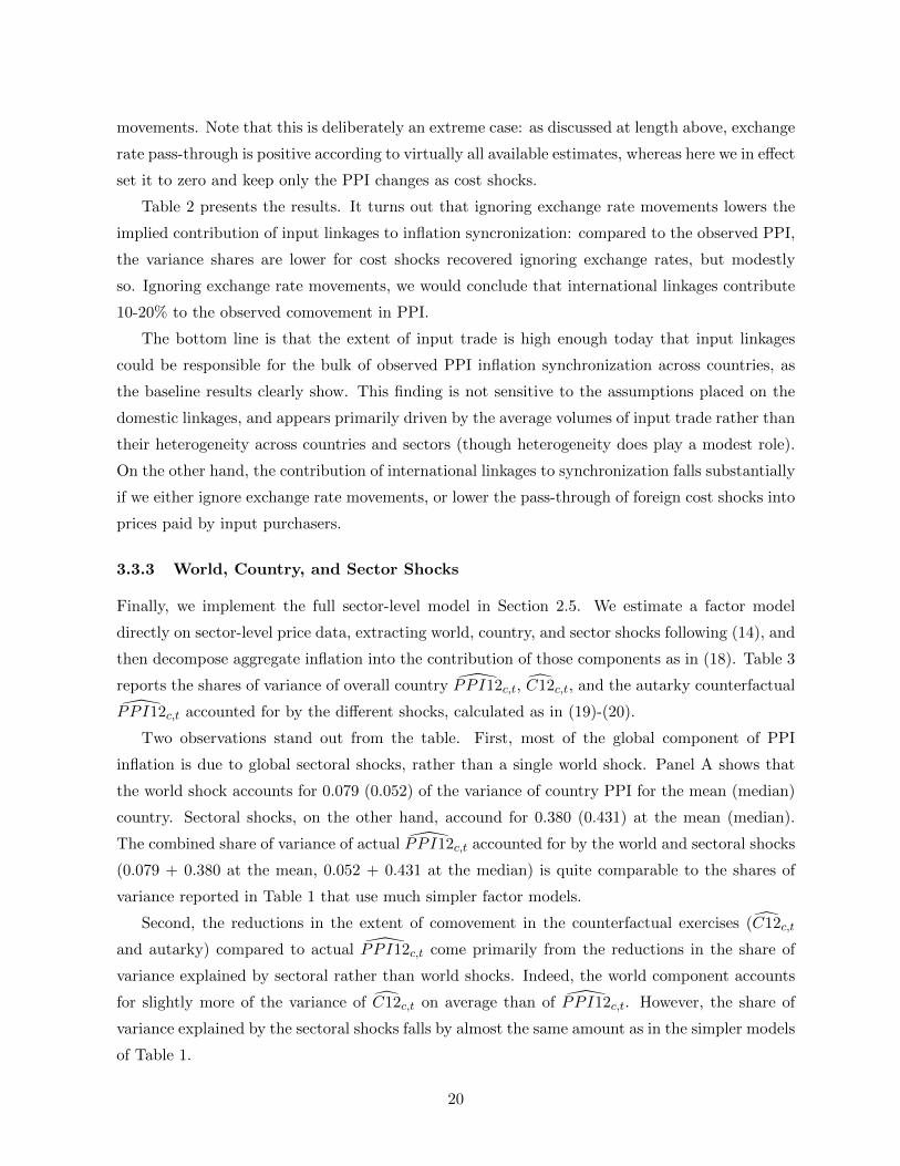
3.3.3 World, Country, and Sector Shocks

Finally, we implement the full sector-level model in Section 2.5. We estimate a factor model

directly on sector-level price data, extracting world, country, and sector shocks following (14), and

then decompose aggregate inflation into the contribution of those components as in (18). Table 3

reports the shares of variance of overall country PP I12c,t, C12c,t, and the autarky counterfactual

PP I12c,t accounted for by the different shocks, calculated as in (19)-(20).

Two observations stand out from the table. First, most of the global component of PPI

inflation is due to global sectoral shocks, rather than a single world shock. Panel A shows that

the world shock accounts for 0.079 (0.052) of the variance of country PPI for the mean (median)

country. Sectoral shocks, on the other hand, accound for 0.380 (0.431) at the mean (median).

The combined share of variance of actual PP I12c,t accounted for by the world and sectoral shocks

(0.079 + 0.380 at the mean, 0.052 + 0.431 at the median) is quite comparable to the shares of

variance reported in Table 1 that use much simpler factor models.

Second, the reductions in the extent of comovement in the counterfactual exercises (C12c,t

and autarky) compared to actual PP I12c,t come primarily from the reductions in the share of

variance explained by sectoral rather than world shocks. Indeed, the world component accounts

for slightly more of the variance of C12c,t on average than of PP I12c,t. However, the share of

variance explained by the sectoral shocks falls by almost the same amount as in the simpler models

of Table 1.

20

These results suggest that common sectoral shocks are the primary driver of PPI synchro-

nization across countries, and that input linkages amplify comovement primarily by propagating

sectoral shocks across countries.

4 Input Linkages and Inflation Tail Risks

As our third and final exercise, we examine to what extent international linkages shape, emphasize,

or dampen the distribution of country inflation. Working with output data, Acemoglu et al. (2015)

emphasize that input-output linkages can generate macroeconomic tail risks if the structure of

the input-output matrix is such that a few sectors play a disproportionately important role as

input suppliers. In this section, we perform a related exercise by asking whether the observed

world input-output linkages are such as to create tail risks in the inflation series.

Figure 8(a) presents the quantile-quantile (Q-Q) plot of the PPI series, standardized to have

mean zero and standard deviation of one in each country versus the standard normal distribution.

Each circle is an observed (standardized) country-year realization of a PPI change. The fact

that observations are above the 45-degree line at the top of the plot, and below at the bottom

indicate that PPI inflation has fatter tails than a normal distribution – large positive and negative

deviations are both more likely than in a normal. Indeed, the conventional tests of normality,

such as Jarque-Bera, Shapiro-Wilk, and D’Agostino-Belanger-D’Agostino tests, reject normality

of PPI with p-values under 0.000. Figure 8(b) presents the Q-Q plot for the recovered costs

shocks, once again standardized to mean zero and standard deviation of one country-by-country.

It appears that the cost shocks are fat-tailed as well, and once again all the formal tests reject

normality with p-values under 0.000.

Acemoglu et al. (2015) prove that when the structure of the input-output matrix is bal-

anced, even fat-failed shocks do not lead to fat-tailed aggregate fluctuations, as shocks are “di-

versified” and a Central Limit Theorem-type result implies that aggregate fluctuations are well-

approximated by a normal distribution. This is clearly not happening in the PPI data: fat-tailed

cost shocks do not “average out” in the input-output structure, and instead lead to fat-tailed PPI

series.

A related question is whether the input-output linkages amplify or dampen the cost shocks.

To check for this, Figure 9 presents the Q-Q plot of the standardized PPI against standardized

cost shocks. Save for the two observations at the very top of the graph, it seems that the PPI

series is modestly less thick-tailed at the top: the largest positive quantiles of actual PPI inflation

are somewhat smaller than the largest positive cost shock realizations. All in all, however, the

distributions are similar, and thus it does not appear to be the case that the IO structure serves

either a strong amplifying or a dampening role.

21

To check whether this result is driven by this particular sample of shock realizations, Figure

10 instead presents the Q-Q plots that come from the simulated data in which we know the

distribution of shocks. That is, we draw a sample of C repeatedly from a known distribution,

and then compute the resulting changes in PPI by applying the Leontief inverse as in (8). We

then aggregate up to the country level to obtain the resulting country PPI’s, standardize, and

compare to the standard normal. We do this for 2 distributions, Laplace and Normal, and 3

variants of shocks: (i) shocks with standard deviation equal to the observed standard deviation

of the C in the data; (ii) shocks with standard deviation equal to 0.1; (iii) world, country, sector,

and idiosyncratic shocks simulated based on the factor model in Section 2.5.

The Laplace distribution has fatter tails than a Normal. By comparing PPI inflation implied

by the Laplace and the Normal underlying cost shocks, we can establish whether the existing IO

structure preserves the fat-tailed underlying shocks or averages them out. The top two panels

reveal that, indeed, the IO structure preserves fat-tailed shocks. When the cost shocks are Laplace

(Figures 10(a)-10(c)), the resulting country PPI’s have fatter tails than a normal, reminiscent of

Figure 8(a) that depicts the actual PPI distribution. By contrast, when underlying cost shocks

are Normal (Figures 10(d)-10(f)), the resulting country PPI series inherit the absence of fat fails.

We conclude from this exercise that the observed structure of global IO linkages is such that

the fat-tailed cost shocks do not average out, and the observed PPI series inherits the fat tails of

the underlying shock process.

5 Conclusion

Inflation rates are highly synchronized across countries. In our own data on PPI’s for a large

sample of countries, the single common factor explains nearly half of the fluctuations in inflation

in the average country. It is important to understand the reasons for this internationalization of

inflation. This paper evaluates a particular hypothesis: inflation synchronization is at least partly

due to international input linkages. On the one hand, input linkages are strong enough to generate

noticeable inflation spillovers. Under full pass-through, input linkages can account for about half

of the observed inflation comovement. These results are not sensitive to particular assumptions on

either domestic input linkages, or the heterogeneity in the linkages across countries and sectors.

On the other hand, the potency of input linkages decreases significantly when the pass-through

of cost shocks is assumed to be lower. Under a 30% pass-through, input linkages account for only

10–15% of observed comovement. These results underscore the importance of developing reliable

estimates of input price pass-through.

22

References

Acemoglu, Daron, Asuman Ozdaglar, and Alireza Tahbaz-Salehi, “Microeconomic Origins ofMacroeconomic Tail Risks,” January 2015. NBER Working Paper No. 20865.

Amiti, Mary, Oleg Itskhoki, and Jozef Konings, “Importers, Exporters, and Exchange RateDisconnect,” American Economic Review, () July : 1942-1978, July 2014, 104 (7), 1942–1978.

Andrade, Philippe and Marios Zachariadis, “Global vs. local shocks in micro price dynamics,”July 2014. Banque de France WP-365.

Auer, Raphael A. and Raphael S. Schoenle, “Market structure and exchange rate pass-through,”Journal of International Economics, 2016, 98, 60–77.

Beck, Guenter W., Kirstin Hubrich, and Massimiliano Marcellino, “On the Importance of Sectoraland Regional Shocks for Price-Setting,” November 2015. Forthcoming, Journal of AppliedEconometrics.

Bems, Rudolfs and Robert C. Johnson, “Value-Added Exchange Rates,,” October 2012. NBERWorking Paper No. 18498.

and , “Demand for Value Added and Value-Added Exchange Rates,” April 2015.NBER Working Paper No. 21070.

Berman, Nicolas, Philippe Martin, and Thierry Mayer, “How do Different Exporters React toExchange Rate Changes? Theory, Empirics and Aggregate Implications,” Quarterly Journalof Economics, 2012, 127 (1), 437–492.

Bianchi, Francesco and Andrea Civelli, “Globalization and inflation: Evidence from a time-varying VAR,” Review of Economic Dynamics, 2015, 18 (2), 406 – 433.

Boehm, Christoph, Aaron Flaaen, and Nitya Pandalai-Nayar, “Input Linkages and the Trans-mission of Shocks: Firm-Level Evidence from the 2011 Tohoku Earthquake,” October 2014.mimeo, University of Michigan.

Borio, Claudio E. V. and Andrew Filardo, “Globalisation and inflation: New cross-countryevidence on the global determinants of domestic inflation,” May 2007. BIS Working Paper227.

Burstein, Ariel and Nir Jaimovich, “Understanding Movements in Aggregate and Product-LevelReal Exchange Rates.,” 2012. Mimeo, UCLA.

, Christopher Kurz, and Linda L. Tesar, “Trade, Production Sharing, and the InternationalTransmission of Business Cycles,” Journal of Monetary Economics, 2008, 55, 775–795.

Burstein, Ariel T. and Gita Gopinath, “International Prices and Exchange Rates,” in Kenneth Ro-goff Elhanan Helpman and Gita Gopinath, eds., Handbook of International Economics, Vol. 4,Elsevier, 2015, chapter 7, pp. 391 – 451.

Bussiere, Matthieu, Giovanni Callegari, Fabio Ghironi, Giulia Sestieri, and Norihiko Yamano,“Estimating Trade Elasticities: Demand Composition and the Trade Collapse of 2008-2009,”American Economic Journal: Macroeconomics, July 2013, 5 (3), 118–151.

Cavallo, Alberto, Brent Neiman, and Roberto Rigobon, “Currency Unions, Product Introduc-tions, and the Real Exchange Rate,” Quarterly Journal of Economics, May 2014, 129 (2),529–595.

Chib, Siddhartha and Edward Greenberg, “Bayes inference in regression models with ARMA (p,q) errors,” Journal of Econometrics, 1994, 64 (1-2), 183–206.

23

Ciccarelli, Matteo and Benoit Mojon, “Global Inflation,” The Review of Economics and Statistics,August 2010, 92 (3), 524–535.

Corsetti, Giancarlo, Luca Dedola, and Sylvain Leduc, “Optimal Monetary Policy in OpenEconomies,” in Benjamin M. Friedman and Michael Woodford, eds., Handbook of Mone-tary Economics, Vol. 3, Elsevier, 2010, chapter 16, pp. 861–933.

di Giovanni, Julian and Andrei A. Levchenko, “Putting the Parts Together: Trade, VerticalLinkages, and Business Cycle Comovement,” American Economic Journal: Macroeconomics,April 2010, 2 (2), 95–124.

Foerster, Andrew T., Pierre-Daniel G. Sarte, and Mark W. Watson, “Sectoral vs. AggregateShocks: A Structural Factor Analysis of Industrial Production,” Journal of Political Econ-omy, February 2011, 119 (1), 1–38.

Gagnon, Etienne, Benjamin R. Mandel, and Robert J. Vigfusson, “Missing Import Price Changesand Low Exchange Rate Pass-Through,” American Economic Journal: Macroeconomics,April 2014, 6 (2), 156–206.

Goldberg, Linda S. and Jose Manuel Campa, “The Sensitivity of the CPI to Exchange Rates:Distribution Margins, Imported Inputs, and Trade Exposure,” Review of Economics andStatistics, May 2010, 92 (2), 392–407.

Gopinath, Gita and Roberto Rigobon, “Sticky Borders,” Quarterly Journal of Economics, May2008, 123 (2), 531–575.

Jackson, Laura E., M. Ayhan Kose, Christopher Otrok, and Michael T. Owyang, “Specifica-tion and Estimation of Bayesian Dynamic Factor Models: A Monte Carlo Analysis with anApplication to Global House Price Comovement,” in Eric Hillebrand and Siem Jan Koop-man, eds., Advances in Econometrics, Vol. 35, United Kingdom: Emerald Insight, 2015,chapter 15, pp. 361–400.

Johnson, Robert C., “Trade in Intermediate Inputs and Business Cycle Comovement,” AmericanEconomic Journal: Macroeconomics, October 2014, 6 (4), 39–83.

Kose, M. Ayhan and Kei-Mu Yi, “Can the Standard International Business Cycle Model Explainthe Relation Between Trade and Comovement,” Journal of International Economics, March2006, 68 (2), 267–295.

Monacelli, Tommaso and Luca Sala, “The International Dimension of Inflation: Evidence fromDisaggregated Consumer Price Data,” Journal of Money, Credit and Banking, 02 2009, 41(s1), 101–120.

Mumtaz, Haroon and Paolo Surico, “The Transmission of International Shocks: A Factor-Augmented VAR Approach,” Journal of Money, Credit and Banking, February 2009, 41(s1), 71–100.

and , “Evolving International Inflation Dynamics: World And Country-Specific Fac-tors,” Journal of the European Economic Association, 08 2012, 10 (4), 716–734.

, Saverio Simonelli, and Paolo Surico, “International Comovements, Business Cycle andInflation: a Historical Perspective,” Review of Economic Dynamics, January 2011, 14 (1),176–198.

Nakamura, Emi and Jon Steinsson, “Lost in Transit: Product Replacement Bias and Pricing toMarket,” American Economic Review, December 2012, 102 (7), 3277–3316.

Neiman, Brent, “Stickiness, Synchronization, and Passthrough in Intrafirm Trade Prices,” Jour-nal of Monetary Economics, 2010, 57 (3), 295–308.

Patel, Nikhil, Zhi Wang, and Shang-Jin Wei, “Global Value Chains and Effective Exchange Ratesat the Country-Sector Level,” June 2014. NBER Working Paper No. 20236.

24

Timmer, Marcel P., Erik Dietzenbacher, Bart Los, Robert Stehrer, and Gaaitzen J. de Vries, “AnIllustrated User Guide to the World Input–Output Database: the Case of Global AutomotiveProduction,” Review of International Economics, August 2015, 23 (3), 575–605.

25

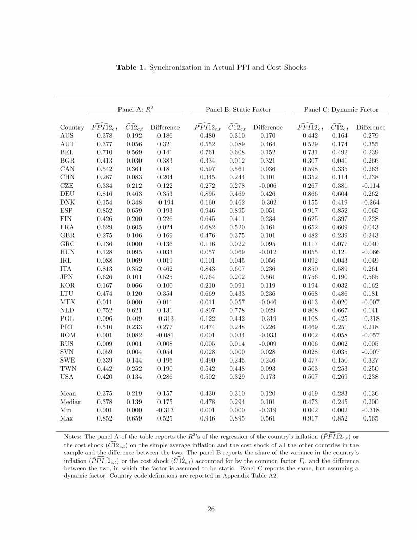
Table 1. Synchronization in Actual PPI and Cost Shocks

Panel A: R2 Panel B: Static Factor Panel C: Dynamic Factor

Country PP I12c,t C12c,t Difference PP I12c,t C12c,t Difference PP I12c,t C12c,t DifferenceAUS 0.378 0.192 0.186 0.480 0.310 0.170 0.442 0.164 0.279AUT 0.377 0.056 0.321 0.552 0.089 0.464 0.529 0.174 0.355BEL 0.710 0.569 0.141 0.761 0.608 0.152 0.731 0.492 0.239BGR 0.413 0.030 0.383 0.334 0.012 0.321 0.307 0.041 0.266CAN 0.542 0.361 0.181 0.597 0.561 0.036 0.598 0.335 0.263CHN 0.287 0.083 0.204 0.345 0.244 0.101 0.352 0.114 0.238CZE 0.334 0.212 0.122 0.272 0.278 -0.006 0.267 0.381 -0.114DEU 0.816 0.463 0.353 0.895 0.469 0.426 0.866 0.604 0.262DNK 0.154 0.348 -0.194 0.160 0.462 -0.302 0.155 0.419 -0.264ESP 0.852 0.659 0.193 0.946 0.895 0.051 0.917 0.852 0.065FIN 0.426 0.200 0.226 0.645 0.411 0.234 0.625 0.397 0.228FRA 0.629 0.605 0.024 0.682 0.520 0.161 0.652 0.609 0.043GBR 0.275 0.106 0.169 0.476 0.375 0.101 0.482 0.239 0.243GRC 0.136 0.000 0.136 0.116 0.022 0.095 0.117 0.077 0.040HUN 0.128 0.095 0.033 0.057 0.069 -0.012 0.055 0.121 -0.066IRL 0.088 0.069 0.019 0.101 0.045 0.056 0.092 0.043 0.049ITA 0.813 0.352 0.462 0.843 0.607 0.236 0.850 0.589 0.261JPN 0.626 0.101 0.525 0.764 0.202 0.561 0.756 0.190 0.565KOR 0.167 0.066 0.100 0.210 0.091 0.119 0.194 0.032 0.162LTU 0.474 0.120 0.354 0.669 0.433 0.236 0.668 0.486 0.181MEX 0.011 0.000 0.011 0.011 0.057 -0.046 0.013 0.020 -0.007NLD 0.752 0.621 0.131 0.807 0.778 0.029 0.808 0.667 0.141POL 0.096 0.409 -0.313 0.122 0.442 -0.319 0.108 0.425 -0.318PRT 0.510 0.233 0.277 0.474 0.248 0.226 0.469 0.251 0.218ROM 0.001 0.082 -0.081 0.001 0.034 -0.033 0.002 0.058 -0.057RUS 0.009 0.001 0.008 0.005 0.014 -0.009 0.006 0.002 0.005SVN 0.059 0.004 0.054 0.028 0.000 0.028 0.028 0.035 -0.007SWE 0.339 0.144 0.196 0.490 0.245 0.246 0.477 0.150 0.327TWN 0.442 0.252 0.190 0.542 0.448 0.093 0.503 0.253 0.250USA 0.420 0.134 0.286 0.502 0.329 0.173 0.507 0.269 0.238

Mean 0.375 0.219 0.157 0.430 0.310 0.120 0.419 0.283 0.136Median 0.378 0.139 0.175 0.478 0.294 0.101 0.473 0.245 0.200Min 0.001 0.000 -0.313 0.001 0.000 -0.319 0.002 0.002 -0.318Max 0.852 0.659 0.525 0.946 0.895 0.561 0.917 0.852 0.565

Notes: The panel A of the table reports the R2’s of the regression of the country’s inflation (PP I12c,t) or

the cost shock (C12c,t) on the simple average inflation and the cost shock of all the other countries in thesample and the difference between the two. The panel B reports the share of the variance in the country’s

inflation (PP I12c,t) or the cost shock (C12c,t) accounted for by the common factor Ft, and the differencebetween the two, in which the factor is assumed to be static. Panel C reports the same, but assuming adynamic factor. Country code definitions are reported in Appendix Table A2.

26

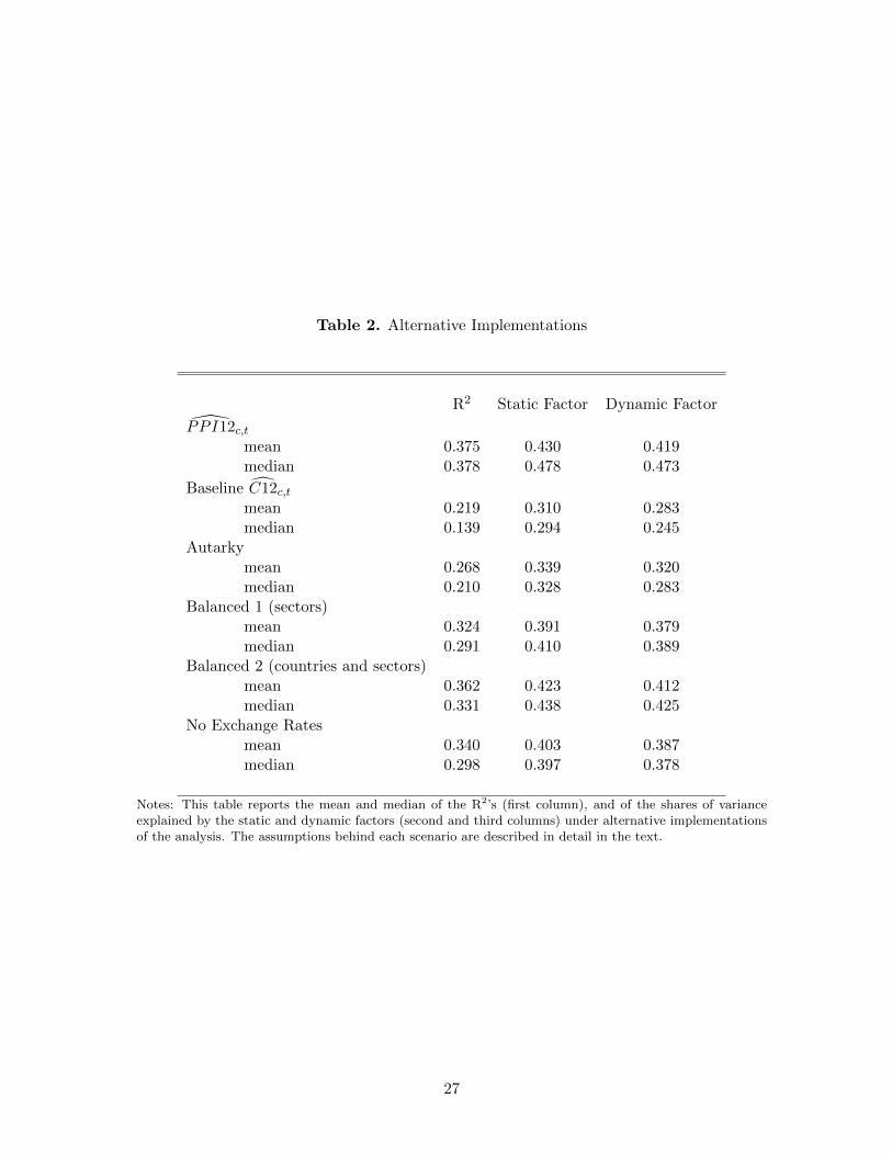
Table 2. Alternative Implementations

R2 Static Factor Dynamic Factor

PP I12c,tmean 0.375 0.430 0.419median 0.378 0.478 0.473

Baseline C12c,tmean 0.219 0.310 0.283median 0.139 0.294 0.245

Autarkymean 0.268 0.339 0.320median 0.210 0.328 0.283

Balanced 1 (sectors)mean 0.324 0.391 0.379median 0.291 0.410 0.389

Balanced 2 (countries and sectors)mean 0.362 0.423 0.412median 0.331 0.438 0.425

No Exchange Ratesmean 0.340 0.403 0.387median 0.298 0.397 0.378

Notes: This table reports the mean and median of the R2’s (first column), and of the shares of varianceexplained by the static and dynamic factors (second and third columns) under alternative implementationsof the analysis. The assumptions behind each scenario are described in detail in the text.

27

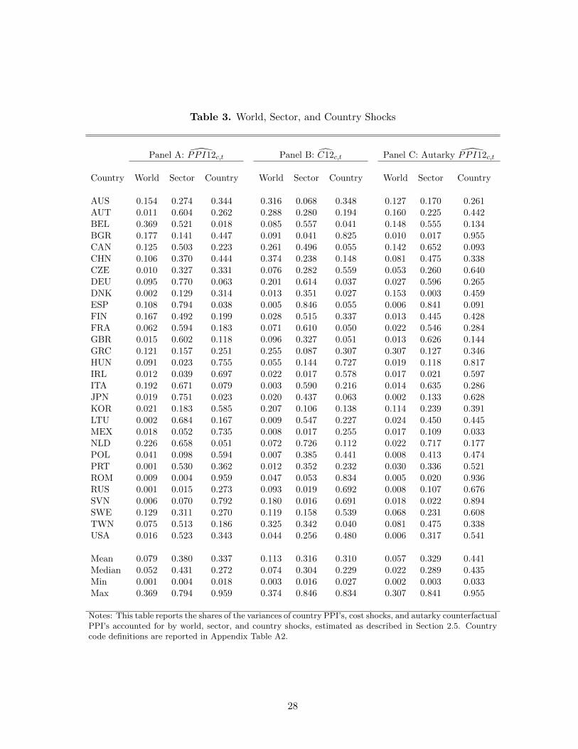
Table 3. World, Sector, and Country Shocks

Panel A: PP I12c,t Panel B: C12c,t Panel C: Autarky PP I12c,t

Country World Sector Country World Sector Country World Sector Country

AUS 0.154 0.274 0.344 0.316 0.068 0.348 0.127 0.170 0.261AUT 0.011 0.604 0.262 0.288 0.280 0.194 0.160 0.225 0.442BEL 0.369 0.521 0.018 0.085 0.557 0.041 0.148 0.555 0.134BGR 0.177 0.141 0.447 0.091 0.041 0.825 0.010 0.017 0.955CAN 0.125 0.503 0.223 0.261 0.496 0.055 0.142 0.652 0.093CHN 0.106 0.370 0.444 0.374 0.238 0.148 0.081 0.475 0.338CZE 0.010 0.327 0.331 0.076 0.282 0.559 0.053 0.260 0.640DEU 0.095 0.770 0.063 0.201 0.614 0.037 0.027 0.596 0.265DNK 0.002 0.129 0.314 0.013 0.351 0.027 0.153 0.003 0.459ESP 0.108 0.794 0.038 0.005 0.846 0.055 0.006 0.841 0.091FIN 0.167 0.492 0.199 0.028 0.515 0.337 0.013 0.445 0.428FRA 0.062 0.594 0.183 0.071 0.610 0.050 0.022 0.546 0.284GBR 0.015 0.602 0.118 0.096 0.327 0.051 0.013 0.626 0.144GRC 0.121 0.157 0.251 0.255 0.087 0.307 0.307 0.127 0.346HUN 0.091 0.023 0.755 0.055 0.144 0.727 0.019 0.118 0.817IRL 0.012 0.039 0.697 0.022 0.017 0.578 0.017 0.021 0.597ITA 0.192 0.671 0.079 0.003 0.590 0.216 0.014 0.635 0.286JPN 0.019 0.751 0.023 0.020 0.437 0.063 0.002 0.133 0.628KOR 0.021 0.183 0.585 0.207 0.106 0.138 0.114 0.239 0.391LTU 0.002 0.684 0.167 0.009 0.547 0.227 0.024 0.450 0.445MEX 0.018 0.052 0.735 0.008 0.017 0.255 0.017 0.109 0.033NLD 0.226 0.658 0.051 0.072 0.726 0.112 0.022 0.717 0.177POL 0.041 0.098 0.594 0.007 0.385 0.441 0.008 0.413 0.474PRT 0.001 0.530 0.362 0.012 0.352 0.232 0.030 0.336 0.521ROM 0.009 0.004 0.959 0.047 0.053 0.834 0.005 0.020 0.936RUS 0.001 0.015 0.273 0.093 0.019 0.692 0.008 0.107 0.676SVN 0.006 0.070 0.792 0.180 0.016 0.691 0.018 0.022 0.894SWE 0.129 0.311 0.270 0.119 0.158 0.539 0.068 0.231 0.608TWN 0.075 0.513 0.186 0.325 0.342 0.040 0.081 0.475 0.338USA 0.016 0.523 0.343 0.044 0.256 0.480 0.006 0.317 0.541

Mean 0.079 0.380 0.337 0.113 0.316 0.310 0.057 0.329 0.441Median 0.052 0.431 0.272 0.074 0.304 0.229 0.022 0.289 0.435Min 0.001 0.004 0.018 0.003 0.016 0.027 0.002 0.003 0.033Max 0.369 0.794 0.959 0.374 0.846 0.834 0.307 0.841 0.955

Notes: This table reports the shares of the variances of country PPI’s, cost shocks, and autarky counterfactualPPI’s accounted for by world, sector, and country shocks, estimated as described in Section 2.5. Countrycode definitions are reported in Appendix Table A2.

28

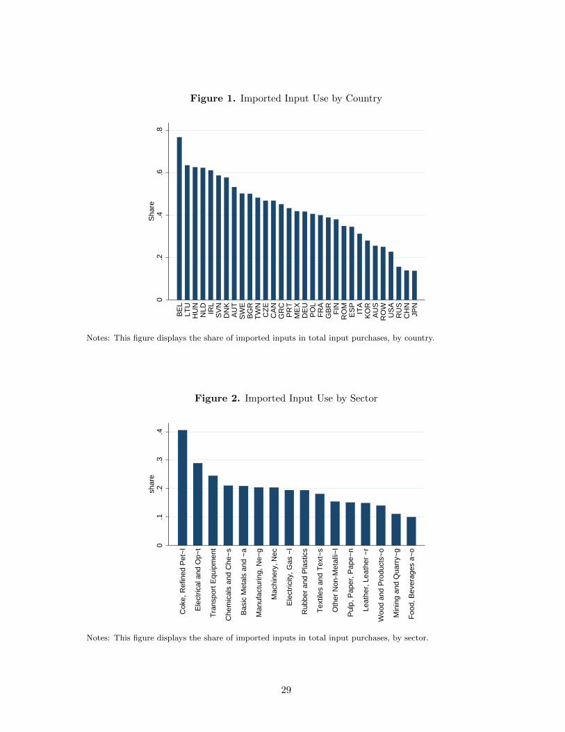
Figure 1. Imported Input Use by Country

0.2

.4.6

.8S

hare

BE

LLT

UH

UN

NLD IR

LS

VN

DN

KA

UT

SW

EB

GR

TW

NC

ZE

CA

NG

RC

PR

TM

EX

DE

UP

OL

FR

AG

BR

FIN

RO

ME

SP

ITA

KO

RA

US

RO

WU

SA

RU

SC

HN

JPN

Notes: This figure displays the share of imported inputs in total input purchases, by country.

Figure 2. Imported Input Use by Sector

0.1

.2.3

.4sh

are

Cok

e, R

efin

ed P

et~

l

Ele

ctric

al a

nd O

p~t

Tra

nspo

rt E

quip

men

t

Che

mic

als

and

Che

~s

Bas

ic M

etal

s an

d ~

a

Man

ufac

turin

g, N

e~g

Mac

hine

ry, N

ec

Ele

ctric

ity, G

as ~

l

Rub

ber

and

Pla

stic

s

Tex

tiles

and

Tex

t~s

Oth

er N

on-M

etal

li~l

Pul

p, P

aper

, Pap

e~n

Leat

her,

Lea

ther

~r

Woo

d an

d P

rodu

cts~

o

Min

ing

and

Qua

rry~

g

Foo

d, B

ever

ages

a~

o

Notes: This figure displays the share of imported inputs in total input purchases, by sector.

29

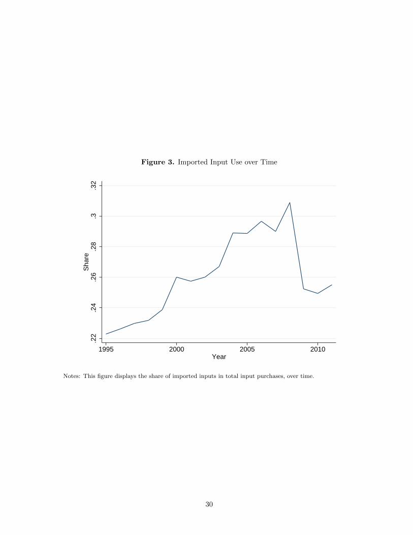
Figure 3. Imported Input Use over Time

.22

.24

.26

.28

.3.3

2S

hare

1995 2000 2005 2010Year

Notes: This figure displays the share of imported inputs in total input purchases, over time.

30

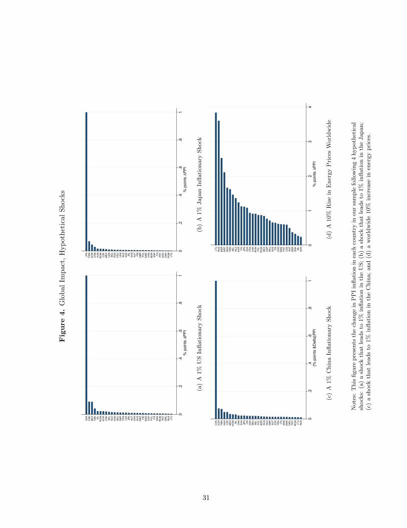
Fig

ure

4.

Glo

bal

Imp

act,

Hyp

oth

etic

alS

hock

s

0.2

.4.6

.81

% p

oin

ts ∆

PP

I

LT

UR

US

GR

CP

RT

RO

MD

NK

ITA

PO

LE

SP

BG

RF

INS

WE

AU

SS

VN

AU

TJP

NC

ZE

FR

AG

BR

DE

UH

UN

NL

DB

EL

CH

NK

OR

RO

WIR

LT

WN

ME

XC

AN

US

A

(a)

A1%

US

Inflati

onary

Shock

0.2

.4.6

.81

% p

oin

ts ∆

PP

I

LT

UR

OM

DN

KG

RC

PR

TIT

AE

SP

BG

RF

RA

SW

EP

OL

GB

RF

INA

UT

SV

NIR

LA

US

NL

DU

SA

DE

UR

US

BE

LC

AN

ME

XC

ZE

RO

WH

UN

CH

NK

OR

TW

NJP

N

(b)

A1%

Japan

Inflati

onary

Shock

0.2

.4.6

.81

{% p

oin

ts &

Delta}P

PI

RU

SL

TU

RO

MP

RT

GR

CS

WE

DN

KIT

AF

RA

ES

PA

UT

GB

RN

LD

AU

SB

GR

PO

LB

EL

DE

UU

SA

FIN

JP

NS

VN

CA

NIR

LR

OW

ME

XC

ZE

HU

NT

WN

KO

RC

HN

(c)

A1%

Chin

aIn

flati

onary

Shock

01

23

4%

poin

ts ∆

PP

I

SV

NIR

LD

NK

GB

RA

UT

CZ

EP

RT

SW

EC

HN

ITA

AU

SD

EU

ES

PM

EX

RO

WP

OL

RO

MC

AN

FR

AU

SA

JP

NF

INK

OR

NL

DB

EL

TW

NH

UN

GR

CB

GR

RU

SL

TU

(d)

A10%

Ris

ein

Ener

gy

Pri

ces

Worl

dw

ide

Note

s:T

his

figure

pre

sents

the

change

inP

PI

inflati

on

inea

chco

untr

yin

our

sam

ple

follow

ing

4hyp

oth

etic

al

shock

s:(a

)a

shock

that

leads

to1%

inflati

on

inth

eU

S;

(b)

ash

ock

that

leads

to1%

inflati

on

inth

eJapan;

(c)

ash

ock

that

leads

to1%

inflati

on

inth

eC

hin

a;

and

(d)

aw

orl

dw

ide

10%

incr

ease

inen

ergy

pri

ces.

31

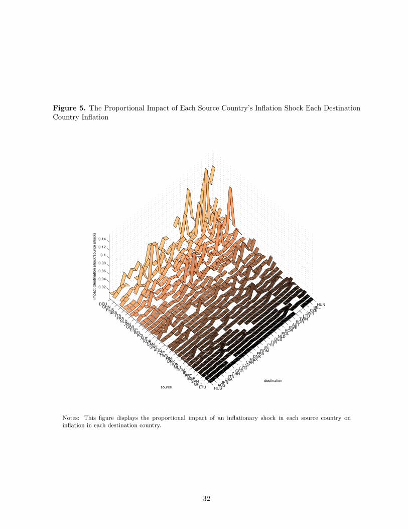
Figure 5. The Proportional Impact of Each Source Country’s Inflation Shock Each DestinationCountry Inflation

LTUGRC

SVNBGR

PRTIRL

ROMMEX

HUNDNK

FINTWN

CZEAUS

SWECAN

KORAUT

POLBEL

ESPGBR

JPNNLD

FRAITA

USARUS

CHNDEU HUN

BELCZE

SVNLTU

TWNBGR

AUTSWE

KORPOL

NLDDEU

FINPRT

IRLROM

FRADNK

MEXCAN

ESPGRC

GBRCHN

ITAUSA

JPNAUS

RUS

0.02

0.04

0.06

0.08

0.1

0.12

0.14

destination

source

impact (d

estination s

hock/s

ourc

e s

hock)

Notes: This figure displays the proportional impact of an inflationary shock in each source country oninflation in each destination country.

32

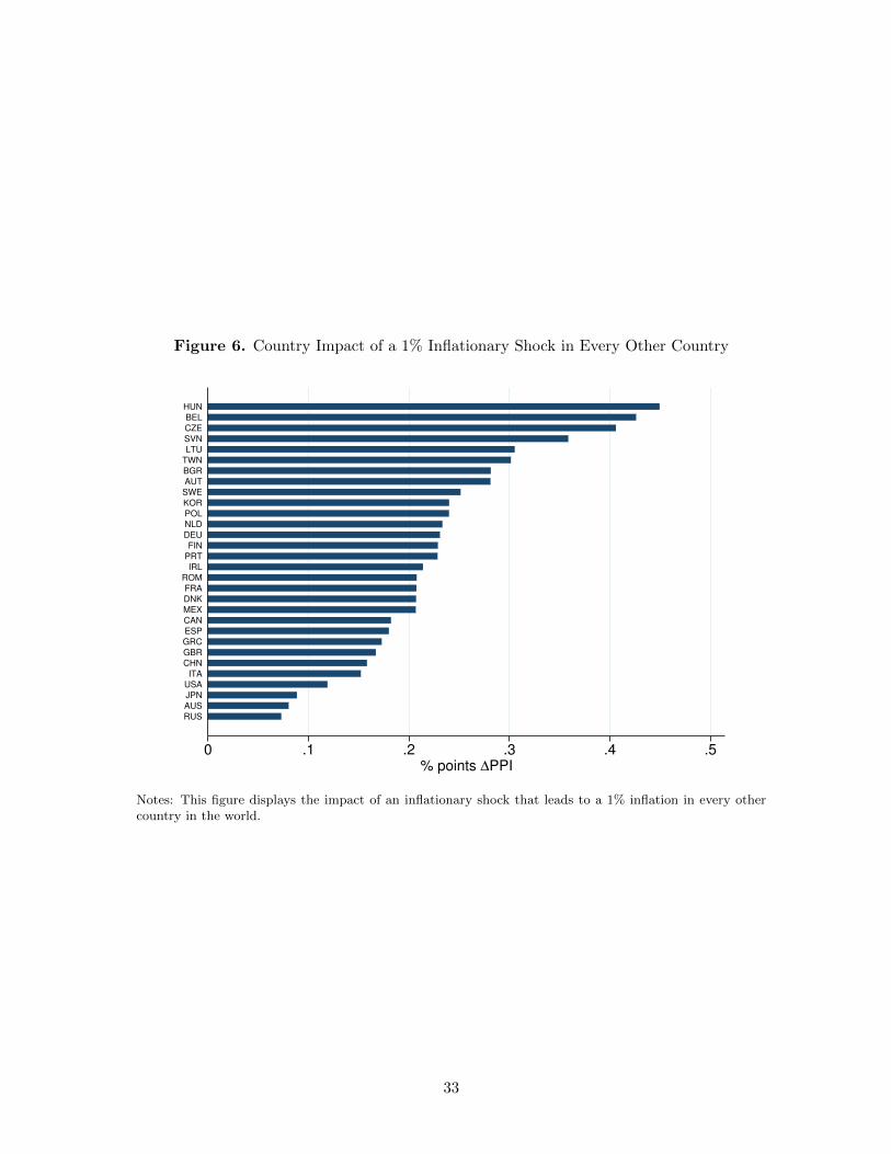
Figure 6. Country Impact of a 1% Inflationary Shock in Every Other Country

0 .1 .2 .3 .4 .5% points ∆PPI

RUS

AUS

JPN

USA

ITA

CHN

GBR

GRC

ESP

CAN

MEX

DNK

FRA

ROM

IRL

PRT

FIN

DEU

NLD

POL

KOR

SWE

AUT

BGR

TWN

LTU

SVN

CZE

BEL

HUN

Notes: This figure displays the impact of an inflationary shock that leads to a 1% inflation in every othercountry in the world.

33

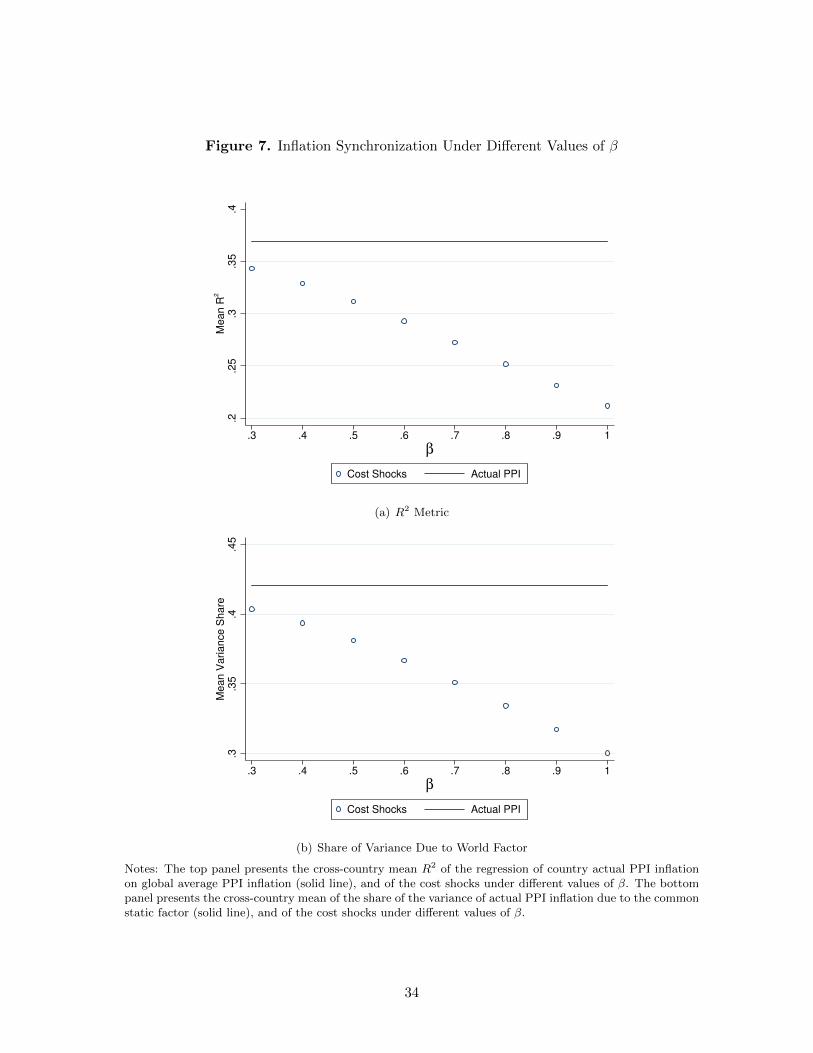
Figure 7. Inflation Synchronization Under Different Values of β

.2.2

5.3

.35

.4M

ean R

2

.3 .4 .5 .6 .7 .8 .9 1

β

Cost Shocks Actual PPI

(a) R2 Metric

.3.3

5.4

.45

Mean V

ariance S

hare

.3 .4 .5 .6 .7 .8 .9 1

β

Cost Shocks Actual PPI

(b) Share of Variance Due to World Factor

Notes: The top panel presents the cross-country mean R2 of the regression of country actual PPI inflationon global average PPI inflation (solid line), and of the cost shocks under different values of β. The bottompanel presents the cross-country mean of the share of the variance of actual PPI inflation due to the commonstatic factor (solid line), and of the cost shocks under different values of β.

34

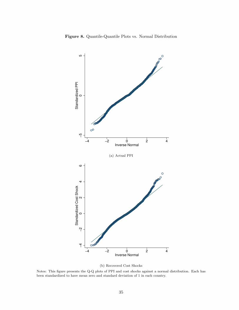
Figure 8. Quantile-Quantile Plots vs. Normal Distribution

−5

05

Sta

ndard

ized P

PI

−4 −2 0 2 4Inverse Normal

(a) Actual PPI

−4

−2

02

46

Sta

ndard

ized C

ost S

hock

−4 −2 0 2 4Inverse Normal

(b) Recovered Cost Shocks

Notes: This figure presents the Q-Q plots of PPI and cost shocks against a normal distribution. Each hasbeen standardized to have mean zero and standard deviation of 1 in each country.

35

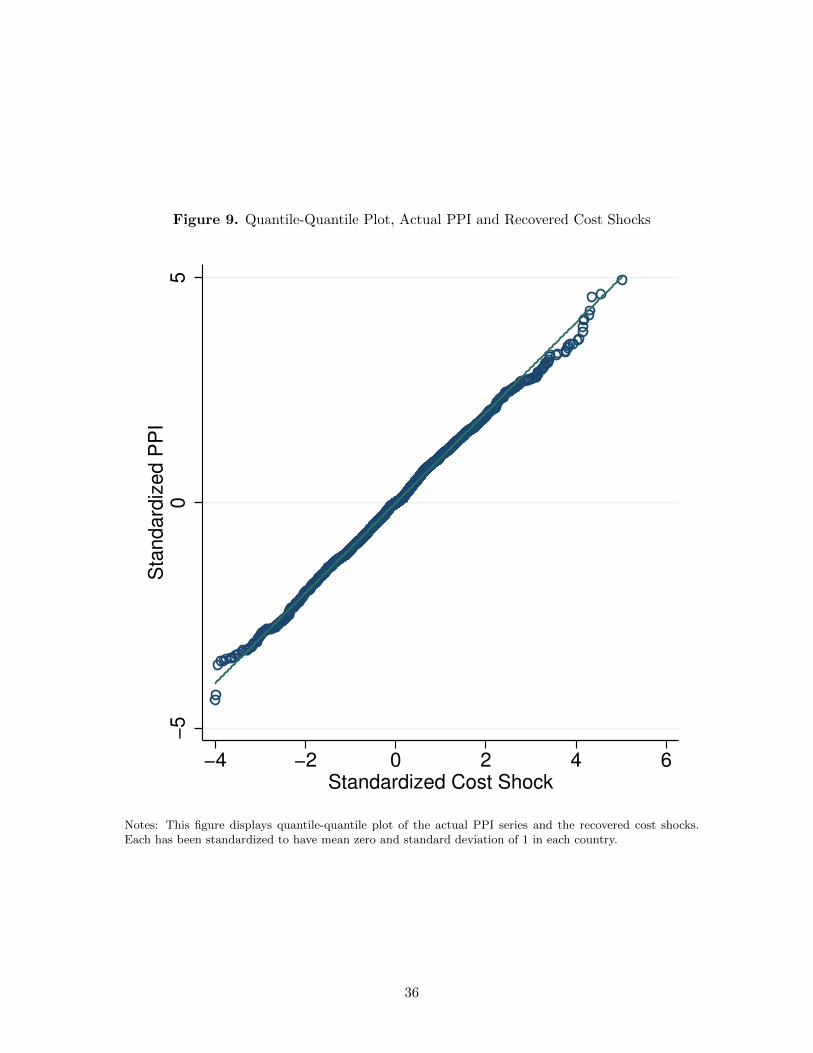
Figure 9. Quantile-Quantile Plot, Actual PPI and Recovered Cost Shocks

−5

05

Sta

nd

ard

ize

d P

PI

−4 −2 0 2 4 6Standardized Cost Shock

Notes: This figure displays quantile-quantile plot of the actual PPI series and the recovered cost shocks.Each has been standardized to have mean zero and standard deviation of 1 in each country.

36

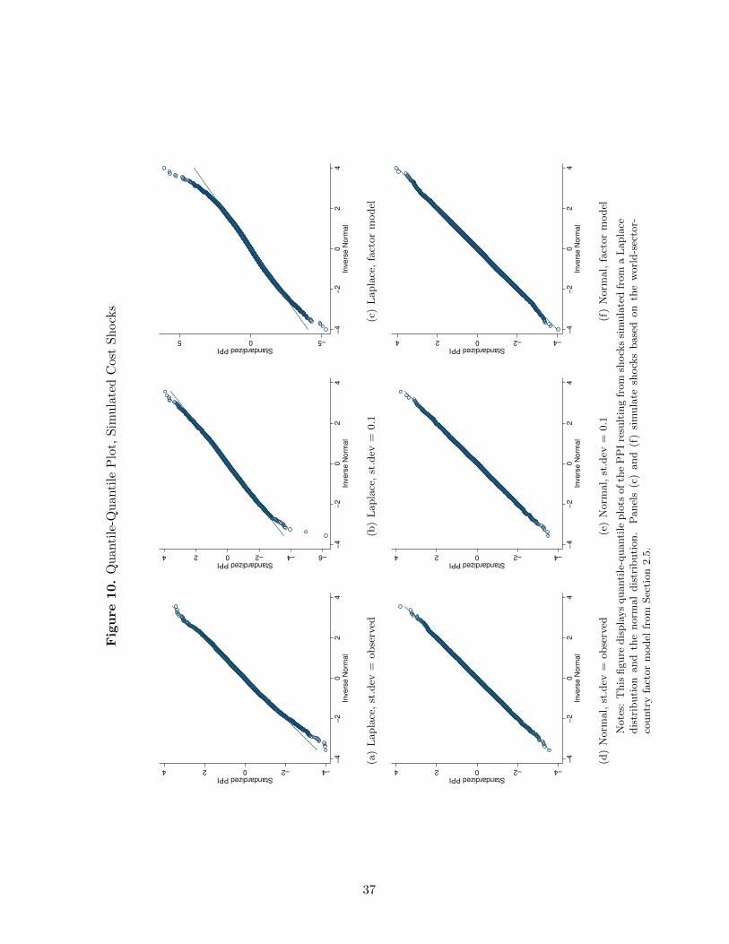
Fig

ure

10.

Qu

anti

le-Q

uan

tile

Plo

t,S

imu

late

dC

ost

Sh

ock

s

−4−2024Standardized PPI

−4

−2

02

4In

vers

e N

orm

al

(a)

Lapla

ce,

st.d

ev=

obse

rved

−6−4−2024Standardized PPI

−4

−2

02

4In

vers

e N

orm

al

(b)

Lapla

ce,

st.d

ev=

0.1

−505Standardized PPI

−4

−2

02

4In

vers

e N

orm

al

(c)

Lapla

ce,

fact

or

model

−4−2024Standardized PPI

−4

−2

02

4In

vers

e N

orm

al

(d)

Norm

al,

st.d

ev=

obse

rved

−4−2024Standardized PPI

−4

−2

02

4In

vers

e N

orm

al

(e)

Norm

al,

st.d

ev=

0.1

−4−2024Standardized PPI

−4

−2

02

4In

vers

e N

orm

al

(f)

Norm

al,

fact

or

model

Note

s:T

his

figure

dis

pla

ys

quanti

le-q

uanti

leplo

tsof

the

PP

Ire

sult

ing

from

shock

ssi

mula

ted

from

aL

apla

cedis

trib

uti

on

and

the

norm

al

dis

trib

uti

on.

Panel

s(c

)and

(f)

sim

ula

tesh

ock

sbase

don

the

worl

d-s

ecto

r-co

untr

yfa

ctor

model

from

Sec

tion

2.5

.

37

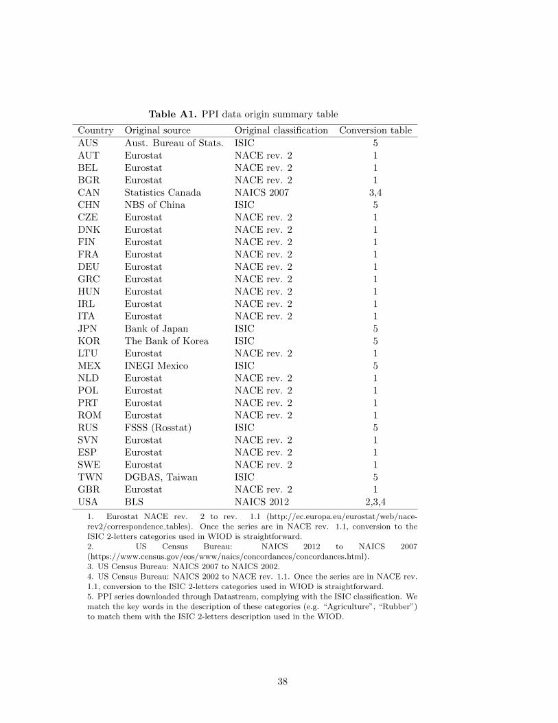
Table A1. PPI data origin summary table

Country Original source Original classification Conversion table

AUS Aust. Bureau of Stats. ISIC 5AUT Eurostat NACE rev. 2 1BEL Eurostat NACE rev. 2 1BGR Eurostat NACE rev. 2 1CAN Statistics Canada NAICS 2007 3,4CHN NBS of China ISIC 5CZE Eurostat NACE rev. 2 1DNK Eurostat NACE rev. 2 1FIN Eurostat NACE rev. 2 1FRA Eurostat NACE rev. 2 1DEU Eurostat NACE rev. 2 1GRC Eurostat NACE rev. 2 1HUN Eurostat NACE rev. 2 1IRL Eurostat NACE rev. 2 1ITA Eurostat NACE rev. 2 1JPN Bank of Japan ISIC 5KOR The Bank of Korea ISIC 5LTU Eurostat NACE rev. 2 1MEX INEGI Mexico ISIC 5NLD Eurostat NACE rev. 2 1POL Eurostat NACE rev. 2 1PRT Eurostat NACE rev. 2 1ROM Eurostat NACE rev. 2 1RUS FSSS (Rosstat) ISIC 5SVN Eurostat NACE rev. 2 1ESP Eurostat NACE rev. 2 1SWE Eurostat NACE rev. 2 1TWN DGBAS, Taiwan ISIC 5GBR Eurostat NACE rev. 2 1USA BLS NAICS 2012 2,3,4

1. Eurostat NACE rev. 2 to rev. 1.1 (http://ec.europa.eu/eurostat/web/nace-rev2/correspondence tables). Once the series are in NACE rev. 1.1, conversion to theISIC 2-letters categories used in WIOD is straightforward.2. US Census Bureau: NAICS 2012 to NAICS 2007(https://www.census.gov/eos/www/naics/concordances/concordances.html).3. US Census Bureau: NAICS 2007 to NAICS 2002.4. US Census Bureau: NAICS 2002 to NACE rev. 1.1. Once the series are in NACE rev.1.1, conversion to the ISIC 2-letters categories used in WIOD is straightforward.5. PPI series downloaded through Datastream, complying with the ISIC classification. Wematch the key words in the description of these categories (e.g. “Agriculture”, “Rubber”)to match them with the ISIC 2-letters description used in the WIOD.

38

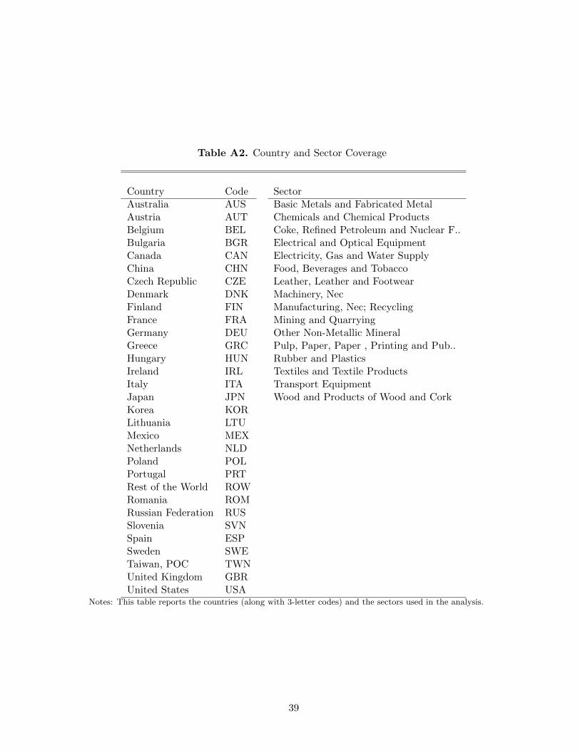
Table A2. Country and Sector Coverage

Country Code SectorAustralia AUS Basic Metals and Fabricated MetalAustria AUT Chemicals and Chemical ProductsBelgium BEL Coke, Refined Petroleum and Nuclear F..Bulgaria BGR Electrical and Optical EquipmentCanada CAN Electricity, Gas and Water SupplyChina CHN Food, Beverages and TobaccoCzech Republic CZE Leather, Leather and FootwearDenmark DNK Machinery, NecFinland FIN Manufacturing, Nec; RecyclingFrance FRA Mining and QuarryingGermany DEU Other Non-Metallic MineralGreece GRC Pulp, Paper, Paper , Printing and Pub..Hungary HUN Rubber and PlasticsIreland IRL Textiles and Textile ProductsItaly ITA Transport EquipmentJapan JPN Wood and Products of Wood and CorkKorea KORLithuania LTUMexico MEXNetherlands NLDPoland POLPortugal PRTRest of the World ROWRomania ROMRussian Federation RUSSlovenia SVNSpain ESPSweden SWETaiwan, POC TWNUnited Kingdom GBRUnited States USA

Notes: This table reports the countries (along with 3-letter codes) and the sectors used in the analysis.

39

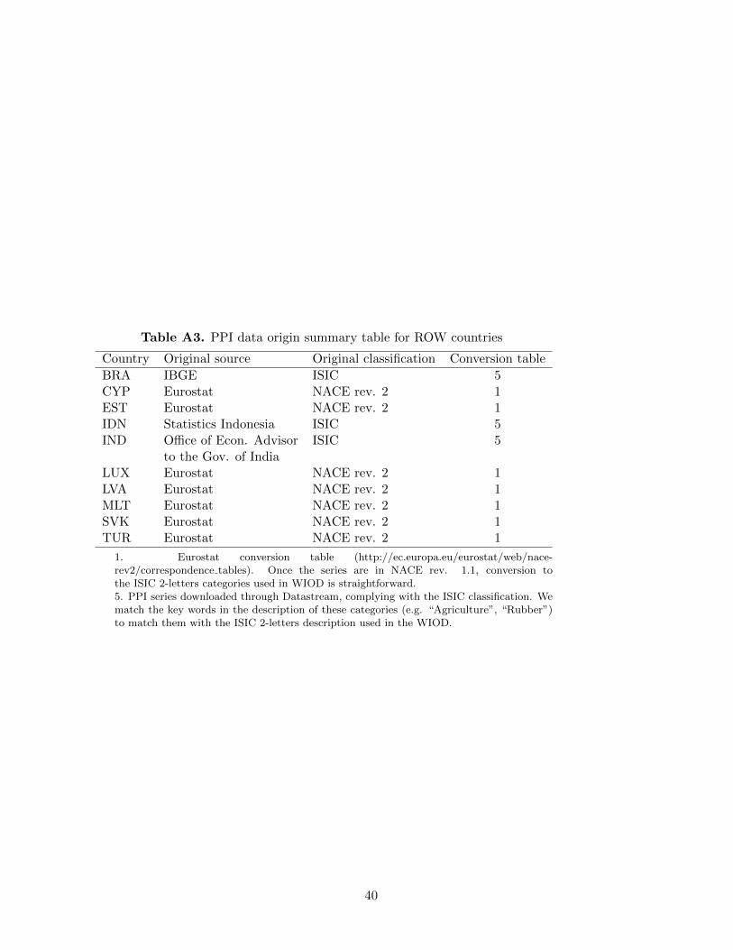
Table A3. PPI data origin summary table for ROW countries

Country Original source Original classification Conversion table

BRA IBGE ISIC 5CYP Eurostat NACE rev. 2 1EST Eurostat NACE rev. 2 1IDN Statistics Indonesia ISIC 5IND Office of Econ. Advisor ISIC 5

to the Gov. of IndiaLUX Eurostat NACE rev. 2 1LVA Eurostat NACE rev. 2 1MLT Eurostat NACE rev. 2 1SVK Eurostat NACE rev. 2 1TUR Eurostat NACE rev. 2 1

1. Eurostat conversion table (http://ec.europa.eu/eurostat/web/nace-rev2/correspondence tables). Once the series are in NACE rev. 1.1, conversion tothe ISIC 2-letters categories used in WIOD is straightforward.5. PPI series downloaded through Datastream, complying with the ISIC classification. Wematch the key words in the description of these categories (e.g. “Agriculture”, “Rubber”)to match them with the ISIC 2-letters description used in the WIOD.

40