Embed Size (px)
Citation preview
Fixed Costs per Shipment∗
Andreas Kropf† Philip Sauré‡
November 2011
Abstract
Exporting firms do not only decide how much of their products they ship
abroad but also at which frequency. Doing so, they face a trade-off between
saving on fixed costs per shipments (by shipping large amounts infrequently)
and saving on storage costs (by delivering just in time with small and fre-
quent shipments). The firm’s optimal choice defines a unique mapping from
size and frequency of shipments to fixed costs of shipment and market entry
cost. We use a unique dataset of Swiss cross-border trade on the transaction
level to analyze the size and shape of the underlying fixed costs. The data
suggest that for Swiss exporters the net present value of fixed costs per ship-
ment are economically important, averaging at about 20 000 CHF. This sum
is equivalent to 0.38 percent of export values or a fifth of market entry cost,
which we estimate to sum to 100 000 CHF. We document that fixed costs
per shipment positively correlate with trade barriers like language common-
alities, trade agreements and distance have the expected sign and realistic
magnitudes.
Keywords: Trade costs, shipment, firm trade.
JEL Classifications: F10.
∗We would like to thank Andreas Fischer, Raphael Auer and seminar participants at the SNB. All remainingerrors are ours. The views expressed in this paper are the authors’ and do not necessarily represent those of the
Swiss National Bank.†A. Kropf, Northwestern University, Evanston, IL, USA. E-mail: [email protected].‡P. Sauré, Swiss National Bank, Börsenstrasse 15, CH-8022 Zurich, Switzerland. E-mail: [email protected].
1 Introduction
Fixed costs of exporting form a centerpiece of the broad literature following Melitz
(2003). These costs divide the set of heterogeneous firms into highly productive
exporters and less productive local sellers, generating rich trade patterns, on the
aggregate and the firm level alike.
Fixed costs of exporting are generally thought to decompose into the fixed costs of
market entry and per-period fixed costs. These two components are equivalent for
trade flows in the static setup that is usually explored.1
In the present paper we introduce and analyze the novel concept of fixed costs per
shipment. Such fixed costs accrue by organizing the collection, insurance and deliv-
ery of goods on a per-shipment basis. Thus, they comprise the monetary equivalent
of the time spent to view and bundle orders, fill in customs forms, monitor and
coordinate the transportation and the arrival at the receiver. Exporting firms can,
for any given quantity of yearly exports, save on fixed costs of shipment by ship-
ping more at a time and paying storage costs at destination. Striking the optimal
trade-off between these costs determines the frequency and the size of shipments as
a function of standard parameters of demand, technology, and interest rates.
Introducing fixed costs per shipment has at least three novel implications. First,
trade theory gains an additional margin through which trade volumes adjust: the
traditional intensive margin (on the firm level) decomposes into frequency and the
size of shipments. Our theory predicts that rises in trade volumes generally come
along with an expansion along both margins: the number of shipments and the value
per shipment. An exception to this general rule occurs when fixed costs per shipment
change. Under such changes, the total trade volume and the number of shipments
increases (decreases), whenever the value per shipment decreases (increases).
Second, the concept of fixed costs per shipment smudges the border between fixed
costs of exporting and variable costs of exporting. Specifically, a distinctive char-
acteristic of fixed costs per shipment is their substitutability with storage costs: a
firm that saves on fixed costs of shipments by shipping more at a time must incur
storage costs at the export destination. The resulting hybrid role of fixed costs per
shipment constitutes a challenge for the Melitz (2003) framework and theoretical
models that rely on the exogenous dichotomy between fix and variable trade costs.
1More precisely, the impact of both types of fixed costs on trade flows is identical as long as
their net present value coincides.
1
Third, the fixed costs per shipment incurred per year are roughly proportional
to trade volumes, since higher trade volumes generally imply a lager number of
shipments. Therefore, fixed costs per shipment are not straight forward to identify.
E.g., empirical work analyzing yearly trade data typically subsumes fixed costs per
shipment under variable transport costs in estimations based on traditional models.
Instead, fixed costs per shipment must be estimated using transaction data, whereas
standard empirical strategies are misfit to capture fixed costs per shipment and thus
tend to underestimate total fixed costs.
In an empirical part, we use transaction-level data from Swiss exporters to quantify
fixed costs per shipment as well as the traditional market entry costs. Our theory
implies that two observable variables - the frequency and the size of shipments -
constitute sufficient statistics to quantify fixed costs of market entry as well as fixed
costs per shipment. Thus, we can infer the fixed costs per shipment purely from
the frequency and value of shipments of single firms. The inferred fixed costs per
shipment are economically important: on average, their net present value is about
20 000 CHF, which translates into a tariff-equivalent of 0.38% or about a fifth of
fixed costs of exporting.
We further exploit the country variation of our data to estimate the impact of some
standard determinants of trade costs: language commonalities, trade agreements
and distance. All of these determinants have a significant impact on the fixed costs
per shipment. Thus, a common language is associated with a 43% reduction, trade
agreements a 35% reduction and finally, the doubling of bilateral distance with a
6% increase in fixed costs per shipment. In our estimations we control for market
size and per capita income, both common determinants of trade flows. Consistent
with our theory, however, we do not find a significant impact of these controls on
fixed costs per shipment.
The impact of the traditional trade barriers on fixed costs of exporting seem rather
modest in comparison: our estimates indicate a somewhat smaller of language com-
monalities (-18%) and trade agreements (-14%) on fixed costs of market entry, while
impact of distance is larger (+13% at a doubling of distance). Overall, market en-
try cost is estimated to be between 100 000 and 1500 000 CHF, which is somewhat
smaller but in the realm of the estimates by Das et al (2007) for Columbian ex-
porters.
Finally, our data allow us to estimate whether the transportation mode correlates
with the fixed costs per shipment. Reading the results with due caution, the analysis
2
suggests that transportation per rail and per ship are associated with very high fixed
costs per shipment compared to those fixed costs for transactions on the road.
Quite generally, the structure of trade costs is important. Since the seminal work by
Melitz (2003), trade economists can no longer ignore the different role of fixed costs
of trade for trade patterns. With the current paper, we specifically argue that the
distinction between fixed costs of market entry and fixed costs per shipment touches
upon a list of key aspects of the new New Trade literature.
First, we add to the literature highlighting the different economic consequences
of the various types of fixed costs of trade. Originally, Melitz (2003) writes that
"...firms are indifferent between paying the one time investment cost , or paying
the amortized per-period portion of this cost = in every period..." ( being
the effective discount rate). Chaney (2005), however, points out that out of steady
state "it does matter whether the fixed costs of exporting is paid once and for all or
at the beginning of each period" and studies the effect of per-period fixed costs on
the transitional dynamics of trade liberalization. Ruhl (2008) studies the different
responses of trade to transitory and permanent shocks to the terms of trade, heavily
relying on the assumption that fixed costs are payed up front. Segura-Cayuela and
Vilarrubia (2008) present a model with learning about an ex-ante "unknown per-
period cost of presence in the foreign market." In a related paper, Irarrazabal and
Opromolla (2009) assume per-period fixed costs to study exporters dynamics under
persistent productivity shocks. Burnstein and Melitz (2011) explore the role of sunk
costs for the dynamics in response to trade liberalization, generally concluding that
macroeconomic dynamics "can vary greatly over time depending on those modeling
ingredients." In the present paper we show that per-period fixed costs can neither
be subsumed under fixed costs of market entry nor can the interval between two
shipments be assumed to be exogenous. Instead, firms adapt the time between two
shipments continuously according to the market conditions.
Second, the literature following Melitz (2003) makes strong assumptions on the
shape of trade costs. Again, Melitz (2003) writes "that the combination of fix
and variable trade costs are high enough to generate partitioning, and therefore
that −1 ." (The parameters , , and stand for variable trade costs,
substitution elasticity between varieties, fixed costs of export market entry and
setup costs of the original plant, respectively.) Direct measures of trade costs as
the cif/fob ratio typically subsume the fixed costs per shipment under variable
transportation costs. Such erroneous accounting can bias the expression on right of
3
the key inequality −1 and lead to flawed estimates. Our analysis emphasizes
that the ratio between fix and variable trade costs is indeed the equilibrium outcome
of firm optimization regarding transport cost minimization and should be treated
as such.
Third, by endogenizing the time between either two shipments for a given firm and
export market, we underscore that the definition of a firm’s exporter status must
rely on a adequate choice of the corresponding time horizon. E.g., firms that ship
products only twice a year report zero exports at least every second quarter. This ob-
servation raises the question whether such firms should be considered non-exporters
every second quarter. That question is central for the literature measuring fixed
costs of (re-) entry to export markets. Das et al (2007) write that exporters "tend
to continue exporting when their current net profits are negative, thus avoiding the
costs of reestablishing themselves in foreign markets when conditions improve." To
properly assess such strategic firm decisions, one needs to know the extent to which
exporters typically stretch the time between two shipments and the trade-offs they
face in doing so. Our analytical framework enables us to address this issue. Looking
at the distribution of the number of yearly shipments suggests that the definition
of exporter status with yearly data is save, while quarterly and monthly data are
inept for most good-country pairs. Moreover, our estimates indicate that the fixed
costs per shipment is gradually increasing with the time since the last shipment so
that the strategic decision to ’stay active in the market’ should affect firms at each
point in time.
Finally, the current paper relates to Armenter and Koren (2010), who analyze trade
patterns when firms randomly fire their shipments to export markets. While the
authors match impressively many patterns of trade data, the authors disregard
the endogeneity of frequency and size of shipments by imposing constant size of
transactions. By focussing exactly on the trade-off between frequency and size
of shipments, the current paper’s approach is diametrically opposed to that by
Armenter and Koren (2010).
About a decade ago, the continuous rise of trade volumes and a secular decline of
tariffs and measured transport costs suggested that trade costs were dead. Baier and
Bergstrand (2001) drew renewed attention to trade barriers by highlighting their role
as a determinant of the rise in global trade volumes. Shortly after, Anderson and
van Wincoop (2004) put forward that trade costs are still substantial in absolute
size and in terms of economic impact. Recognizing the importance of trade cost
4

Jacks, Meissner and Novy (2008) and Novy (2011) offer a novel measure of bilateral
trade costs and disentangled parallel but distinct dynamics of bilateral trade costs.
The present paper adds to this literature by estimating the different components of
trade costs and their respective determinants.
Relating to the crucial assumptions of the Melitz model, other research has ad-
dressed the type and nature of trade cost. Das et al (2007) structurally estimate
the fixed costs of entry to foreign markets. The authors find that "[a]mong small pro-
ducers, average entry costs range from $430,000 U.S. dollars [...] to [...] $412,000."
The corresponding numbers for large producers are $344,000 to $402,000. Com-
pared to these substantial numbers, the authors report that annual fixed costs of
exporting are close to zero. Anderson and Yotov (2010) have recently analyzed the
proportions of trade costs paid by sellers and buyers, showing that the incidence of
trade costs has important implications for the home bias, the disproportionate pre-
dicted share of local trade and the gains from trade. We connect to this literature
by introducing the distinction of two different types of fixed costs of trade and by
providing the framework to assess them.
The remainder of the paper is structured as follows. Section 2 presents the theo-
retical model. Section 3 describes the Swiss trade date, which we use to test our
theory in Section 4. Finally, Section 5 concludes.
2 The Model
We develop a framework that incorporates the frequency of exports as an endoge-
nous choice variable of firms in a standard Melitz-type model of heterogeneous
firms. Doing so, we focus on an static setup, assuming in particular that population
sizes, technologies and trade barriers, and consequently output and trade flows are
constant.
2.1 Preferences
Consider a world with countries, indexed by = 1 2 . Every country pro-
duces and consumes a continuum of products. Country ’s flow utility function
5
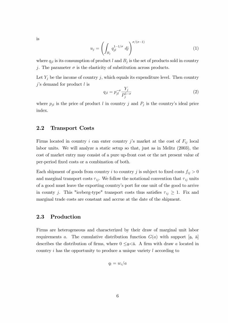
is
=
ÃZ
1−1
!(−1)
(1)
where is its consumption of product and is the set of products sold in country
. The parameter is the elasticity of substitution across products.
Let be the income of country , which equals its expenditure level. Then country
’s demand for product is
= −
1−
(2)
where is the price of product in country and is the country’s ideal price
index.
2.2 Transport Costs
Firms located in country can enter country ’s market at the cost of local
labor units. We will analyze a static setup so that, just as in Melitz (2003), the
cost of market entry may consist of a pure up-front cost or the net present value of
per-period fixed costs or a combination of both.
Each shipment of goods from country to country is subject to fixed costs 0
and marginal transport costs . We follow the notational convention that units
of a good must leave the exporting country’s port for one unit of the good to arrive
in county . This "iceberg-type" transport costs thus satisfies ≥ 1. Fix and
marginal trade costs are constant and accrue at the date of the shipment.
2.3 Production
Firms are heterogeneous and characterized by their draw of marginal unit labor
requirements . The cumulative distribution function () with support [a¯, a]
describes the distribution of firms, where 0 ≤a¯a. A firm with draw located in
country has the opportunity to produce a unique variety according to
=
6
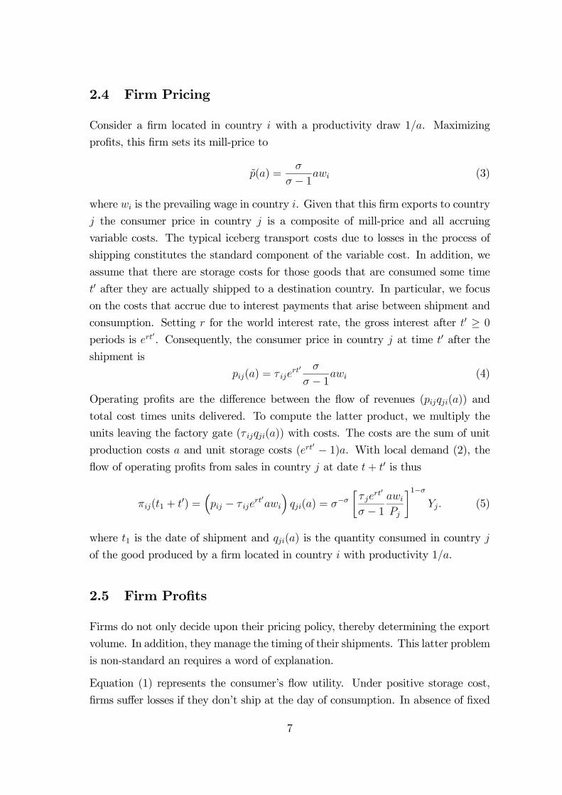
2.4 Firm Pricing
Consider a firm located in country with a productivity draw 1. Maximizing
profits, this firm sets its mill-price to
() =
− 1 (3)
where is the prevailing wage in country . Given that this firm exports to country
the consumer price in country is a composite of mill-price and all accruing
variable costs. The typical iceberg transport costs due to losses in the process of
shipping constitutes the standard component of the variable cost. In addition, we
assume that there are storage costs for those goods that are consumed some time
0 after they are actually shipped to a destination country. In particular, we focus
on the costs that accrue due to interest payments that arise between shipment and
consumption. Setting for the world interest rate, the gross interest after 0 ≥ 0periods is
0. Consequently, the consumer price in country at time 0 after the
shipment is
() = 0
− 1 (4)
Operating profits are the difference between the flow of revenues (()) and
total cost times units delivered. To compute the latter product, we multiply the
units leaving the factory gate ( ()) with costs. The costs are the sum of unit
production costs and unit storage costs (0 − 1). With local demand (2), the
flow of operating profits from sales in country at date + 0 is thus
(1 + 0) =³ −
0
´() = −
∙
0
− 1
¸1− (5)
where 1 is the date of shipment and () is the quantity consumed in country
of the good produced by a firm located in country with productivity 1.
2.5 Firm Profits
Firms do not only decide upon their pricing policy, thereby determining the export
volume. In addition, they manage the timing of their shipments. This latter problem
is non-standard an requires a word of explanation.
Equation (1) represents the consumer’s flow utility. Under positive storage cost,
firms suffer losses if they don’t ship at the day of consumption. In absence of fixed
7
costs of shipment, a firm would therefore send a flow of shipments to the destination
countries so that its products arrive precisely at the date of consumption.2 In
presence of fixed costs of shipment, however, such a strategy is infinitely costly, since
at each infinitesimal date a discrete cost would arise. Consequently, shipments are
discrete.
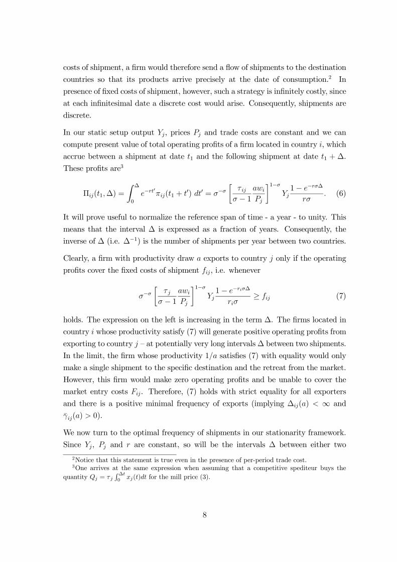
In our static setup output , prices and trade costs are constant and we can
compute present value of total operating profits of a firm located in country , which
accrue between a shipment at date 1 and the following shipment at date 1 + ∆.
These profits are3
Π(1∆) =
Z ∆
0
−0(1 + 0) 0 = −
∙
− 1
¸1−1− −∆
(6)
It will prove useful to normalize the reference span of time - a year - to unity. This
means that the interval ∆ is expressed as a fraction of years. Consequently, the
inverse of ∆ (i.e. ∆−1) is the number of shipments per year between two countries.
Clearly, a firm with productivity draw exports to country only if the operating
profits cover the fixed costs of shipment , i.e. whenever
−∙
− 1
¸1−1− −∆
≥ (7)
holds. The expression on the left is increasing in the term ∆. The firms located in
country whose productivity satisfy (7) will generate positive operating profits from
exporting to country — at potentially very long intervals∆ between two shipments.
In the limit, the firm whose productivity 1 satisfies (7) with equality would only
make a single shipment to the specific destination and the retreat from the market.
However, this firm would make zero operating profits and be unable to cover the
market entry costs . Therefore, (7) holds with strict equality for all exporters
and there is a positive minimal frequency of exports (implying ∆() ∞ and
() 0).
We now turn to the optimal frequency of shipments in our stationarity framework.
Since , and are constant, so will be the intervals ∆ between either two
2Notice that this statement is true even in the presence of per-period trade cost.3One arrives at the same expression when assuming that a competitive spediteur buys the
quantity = R∆0
() for the mill price (3).
8
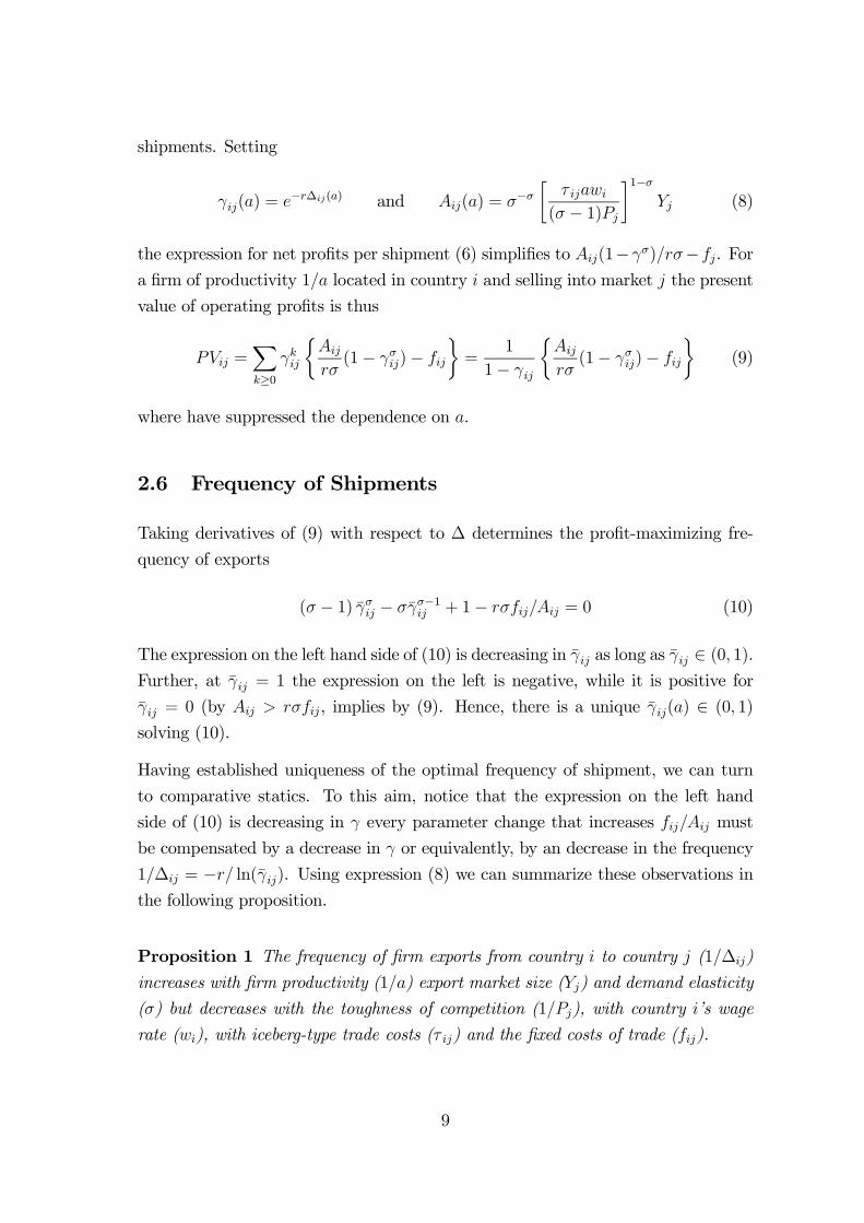
shipments. Setting
() = −∆() and () = −∙
( − 1)
¸1− (8)
the expression for net profits per shipment (6) simplifies to (1−)−. For
a firm of productivity 1 located in country and selling into market the present
value of operating profits is thus
=X≥0
½
(1− )−
¾=
1
1−
½
(1− )−
¾(9)
where have suppressed the dependence on .
2.6 Frequency of Shipments
Taking derivatives of (9) with respect to ∆ determines the profit-maximizing fre-
quency of exports
( − 1) − −1 + 1− = 0 (10)
The expression on the left hand side of (10) is decreasing in as long as ∈ (0 1).Further, at = 1 the expression on the left is negative, while it is positive for
= 0 (by , implies by (9). Hence, there is a unique () ∈ (0 1)solving (10).
Having established uniqueness of the optimal frequency of shipment, we can turn
to comparative statics. To this aim, notice that the expression on the left hand
side of (10) is decreasing in every parameter change that increases must
be compensated by a decrease in or equivalently, by an decrease in the frequency
1∆ = − ln(). Using expression (8) we can summarize these observations inthe following proposition.
Proposition 1 The frequency of firm exports from country to country (1∆)
increases with firm productivity (1) export market size () and demand elasticity
() but decreases with the toughness of competition (1), with country ’s wage
rate (), with iceberg-type trade costs ( ) and the fixed costs of trade ().
9
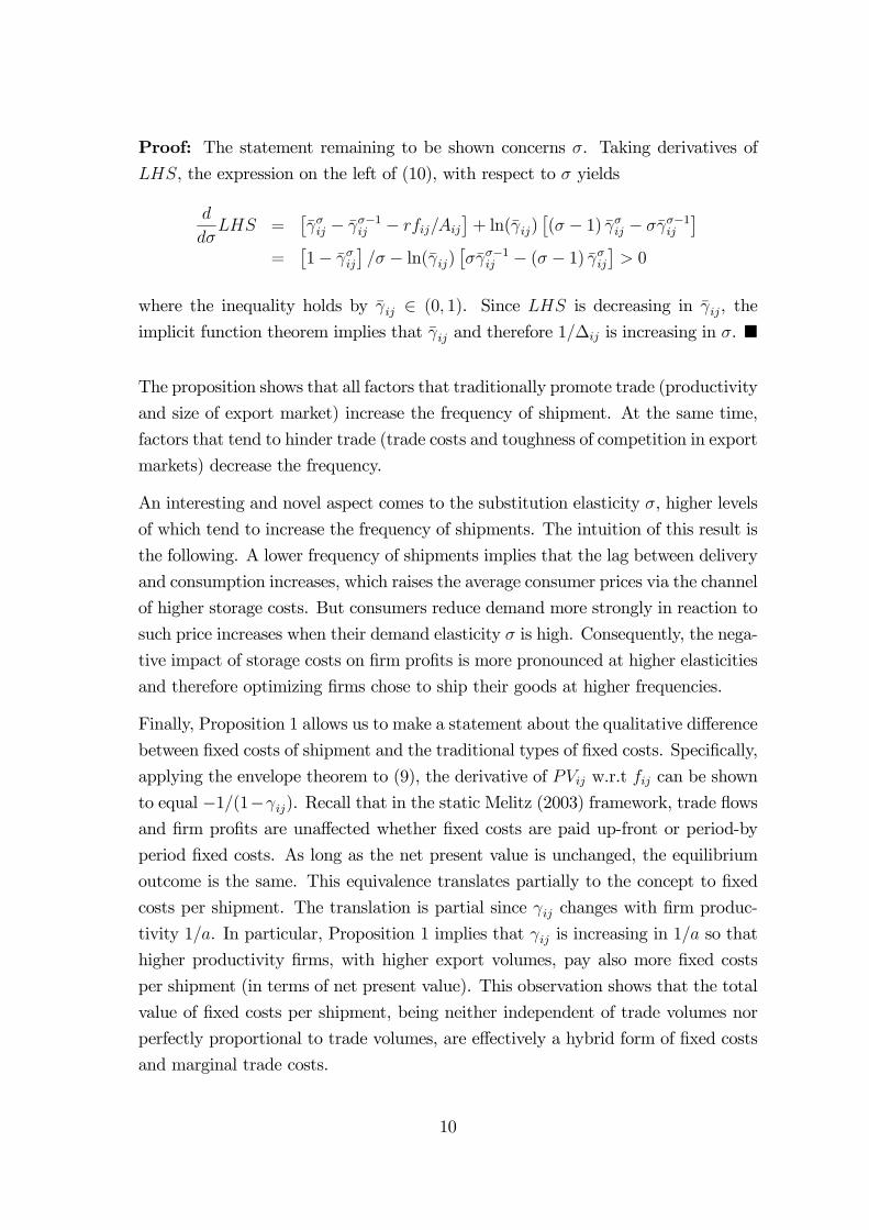
Proof: The statement remaining to be shown concerns . Taking derivatives of
, the expression on the left of (10), with respect to yields
=
£ − −1 −
¤+ ln()
£( − 1) − −1
¤=
£1−
¤ − ln()
£−1 − ( − 1)
¤ 0
where the inequality holds by ∈ (0 1). Since is decreasing in , the
implicit function theorem implies that and therefore 1∆ is increasing in . ¥
The proposition shows that all factors that traditionally promote trade (productivity
and size of export market) increase the frequency of shipment. At the same time,
factors that tend to hinder trade (trade costs and toughness of competition in export
markets) decrease the frequency.
An interesting and novel aspect comes to the substitution elasticity , higher levels
of which tend to increase the frequency of shipments. The intuition of this result is
the following. A lower frequency of shipments implies that the lag between delivery
and consumption increases, which raises the average consumer prices via the channel
of higher storage costs. But consumers reduce demand more strongly in reaction to
such price increases when their demand elasticity is high. Consequently, the nega-
tive impact of storage costs on firm profits is more pronounced at higher elasticities
and therefore optimizing firms chose to ship their goods at higher frequencies.
Finally, Proposition 1 allows us to make a statement about the qualitative difference
between fixed costs of shipment and the traditional types of fixed costs. Specifically,
applying the envelope theorem to (9), the derivative of w.r.t can be shown
to equal −1(1−). Recall that in the static Melitz (2003) framework, trade flowsand firm profits are unaffected whether fixed costs are paid up-front or period-by
period fixed costs. As long as the net present value is unchanged, the equilibrium
outcome is the same. This equivalence translates partially to the concept to fixed
costs per shipment. The translation is partial since changes with firm produc-
tivity 1. In particular, Proposition 1 implies that is increasing in 1 so that
higher productivity firms, with higher export volumes, pay also more fixed costs
per shipment (in terms of net present value). This observation shows that the total
value of fixed costs per shipment, being neither independent of trade volumes nor
perfectly proportional to trade volumes, are effectively a hybrid form of fixed costs
and marginal trade costs.
10
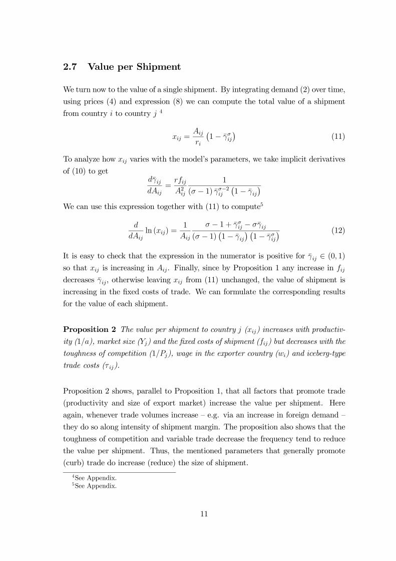
2.7 Value per Shipment
We turn now to the value of a single shipment. By integrating demand (2) over time,
using prices (4) and expression (8) we can compute the total value of a shipment
from country to country 4
=
¡1−
¢(11)
To analyze how varies with the model’s parameters, we take implicit derivatives
of (10) to get
=
2
1
( − 1) −2
¡1−
¢We can use this expression together with (11) to compute5
ln () =1
− 1 + −
( − 1) ¡1− ¢ ¡1−
¢ (12)
It is easy to check that the expression in the numerator is positive for ∈ (0 1)so that is increasing in . Finally, since by Proposition 1 any increase in
decreases , otherwise leaving from (11) unchanged, the value of shipment is
increasing in the fixed costs of trade. We can formulate the corresponding results
for the value of each shipment.
Proposition 2 The value per shipment to country () increases with productiv-
ity (1), market size () and the fixed costs of shipment () but decreases with the
toughness of competition (1), wage in the exporter country () and iceberg-type
trade costs ( ).
Proposition 2 shows, parallel to Proposition 1, that all factors that promote trade
(productivity and size of export market) increase the value per shipment. Here
again, whenever trade volumes increase — e.g. via an increase in foreign demand —
they do so along intensity of shipment margin. The proposition also shows that the
toughness of competition and variable trade decrease the frequency tend to reduce
the value per shipment. Thus, the mentioned parameters that generally promote
(curb) trade do increase (reduce) the size of shipment.
4See Appendix.5See Appendix.
11
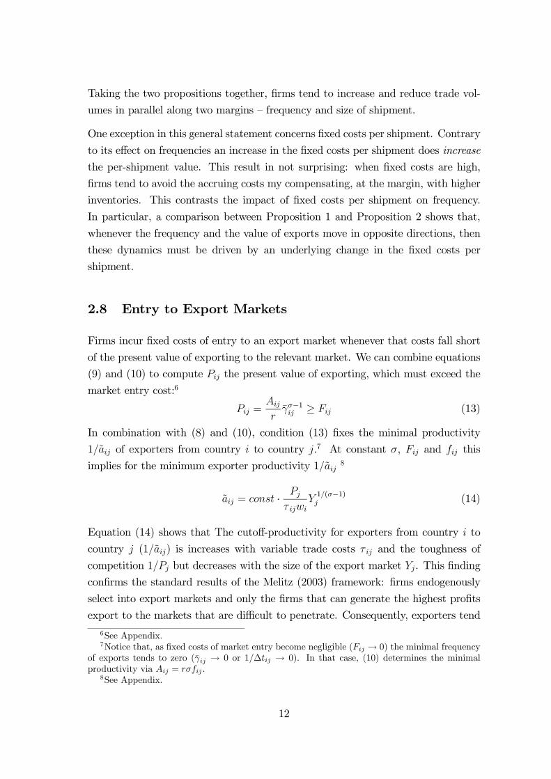
Taking the two propositions together, firms tend to increase and reduce trade vol-
umes in parallel along two margins — frequency and size of shipment.
One exception in this general statement concerns fixed costs per shipment. Contrary
to its effect on frequencies an increase in the fixed costs per shipment does increase
the per-shipment value. This result in not surprising: when fixed costs are high,
firms tend to avoid the accruing costs my compensating, at the margin, with higher
inventories. This contrasts the impact of fixed costs per shipment on frequency.
In particular, a comparison between Proposition 1 and Proposition 2 shows that,
whenever the frequency and the value of exports move in opposite directions, then
these dynamics must be driven by an underlying change in the fixed costs per
shipment.
2.8 Entry to Export Markets
Firms incur fixed costs of entry to an export market whenever that costs fall short
of the present value of exporting to the relevant market. We can combine equations
(9) and (10) to compute the present value of exporting, which must exceed the
market entry cost:6
=
−1 ≥ (13)
In combination with (8) and (10), condition (13) fixes the minimal productivity
1 of exporters from country to country .7 At constant , and this
implies for the minimum exporter productivity 18
= ·
1(−1) (14)
Equation (14) shows that The cutoff-productivity for exporters from country to
country (1) is increases with variable trade costs and the toughness of
competition 1 but decreases with the size of the export market . This finding
confirms the standard results of the Melitz (2003) framework: firms endogenously
select into export markets and only the firms that can generate the highest profits
export to the markets that are difficult to penetrate. Consequently, exporters tend
6See Appendix.7Notice that, as fixed costs of market entry become negligible ( → 0) the minimal frequency
of exports tends to zero ( → 0 or 1∆ → 0). In that case, (10) determines the minimal
productivity via = .8See Appendix.
12
to be the most productive and the corresponding markets the most profitable ones.
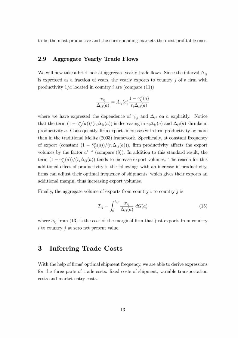
2.9 Aggregate Yearly Trade Flows
We will now take a brief look at aggregate yearly trade flows. Since the interval ∆
is expressed as a fraction of years, the yearly exports to country of a firm with
productivity 1 located in country are (compare (11))
∆()= ()
1− ()
∆()
where we have expressed the dependence of and ∆ on explicitly. Notice
that the term (1− ())(∆()) is decreasing in ∆() and ∆() shrinks in
productivity . Consequently, firm exports increases with firm productivity by more
than in the traditional Melitz (2003) framework. Specifically, at constant frequency
of export (constant (1 − ())(∆())), firm productivity affects the export
volumes by the factor 1− (compare (8)). In addition to this standard result, the
term (1− ())(∆()) tends to increase export volumes. The reason for this
additional effect of productivity is the following: with an increase in productivity,
firms can adjust their optimal frequency of shipments, which gives their exports an
additional margin, thus increasing export volumes.
Finally, the aggregate volume of exports from country to country is
=
Z
0
∆()() (15)
where from (13) is the cost of the marginal firm that just exports from country
to country at zero net present value.
3 Inferring Trade Costs
With the help of firms’ optimal shipment frequency, we are able to derive expressions
for the three parts of trade costs: fixed costs of shipment, variable transportation
costs and market entry costs.
13
3.1 Fixed Costs per Shipment
To derive an expression for the fixed costs per shipment we start by combining the
optimality condition (10) and the value per shipment (11) to eliminate , which
renders
=( − 1) − −1 + 1
1−
(16)
It is noteworthy that the expression of fixed costs per shipment depends neither on
firm productivity, variable trade costs nor on market characteristics of the exporting
or importing country. The only relevant parameters are the value per shipment ,
the frequency∆, the interest rate and the elasticity . In fact, it is intuitive that,
once total trade volume (∆) is known, its decomposition into single shipments
does not depend on characteristics of the countries but exclusively on the parameters
governing the trade-off between higher trade costs ( ) and higher storage costs ().
As discussed in connection with Proposition 1, the elasticity impacts this trade-off
through the consumers’ sensitivity to absorb marginal storage costs. Therefore,
enters expression (16) as well.
In sum, the parameters , and are sufficient to determine the decomposition of
total trade into and ∆ — or reversely, can be inferred from the observables
and ∆, given that and are known.
3.2 Variable Transport Costs
With the expression (8), we can restate (11) as
=
∙
( − 1)
¸1−
¡1−
¢
(17)
which is a version of the gravity equation on the firm level. Notice that in this
expression firm productivity 1 appears explicitly, in contrast to expression () for
fixed costs per shipment. Thus, estimates of the variable trade costs must involve
firm dummies and country dummies as long as firm productivity 1 and ideal price
index are unobserved. Alternatively, estimates could base information about the
marginal costs as in the data used in Das et al (2007).
In sum, and very much in line with the standard Melitz (2003) framework, variable
trade costs can be inferred from trade flows once firm productivity, market size and
the prevailing price index are known.
14
3.3 Market Entry Costs
Since no firm can be expected to have exactly the productivity that makes it the
marginal exporter, the costs of market entry can only be proxied by an upper
bound through (13). Specifically, we can use (11) to reformulate condition (13) as
−1 (1− ) ≥ . Taking logs and exploiting (8) leads to
( − 1)∆ + ln ()− ln(1− ) ≥ ln() (18)
For firms with the cutoff productivity level this inequality binds. Thus, for each
country pair, the lowest value of the expression on the right observed throughout
the universe of exporters constitutes an upper bound on the fixed costs of exporting.
4 Data
4.1 The Universe of Swiss Trade Data
The source of our data is the Swiss Customs (Oberzolldirektion) which records
every legal transaction of cross-border trade. If a pharmaceutical firm sends two
boxes of the same drug to the same destination on the same day, but involving two
different custom forms, then two distinct transactions are recorded. We refer to
these transactions as shipments.
The data span the period between the years 2005 and 2009 and report single cross-
border transactions using an 8-digit goods classification system (tariff number).
Year and month of the transaction are recorded.9 Our core variable is the value of
each shipment in Swiss francs.
We only consider the goods that enter the official Swiss trade statistics — officially
labeled Total 1. This definition excludes precious metals and antique furniture; we
also exclude energy as well as all goods whose type of transportation is recorded as
self-propelled.10 This restriction leaves us with 8036 (8759) goods classes and 243
9Days are reported as well but not reliably so: the majority of shipments are recorded on the
first day of the corresponding month.10Trade in energy comprises all goods transported via pipelines, which are recorded as one
shipment per quarter and classification. Trade of self-propelled goods are in units. The restriction
eliminates 0.204% of all observations for imports and 0.268% for exports. These correspond to
2.9% and 8.31% of export and import values, respectively.
15
(239) countries appearing at least once in the export (import) data over the full
range of five year.
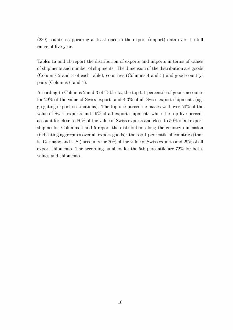
Tables 1a and 1b report the distribution of exports and imports in terms of values
of shipments and number of shipments. The dimension of the distribution are goods
(Columns 2 and 3 of each table), countries (Columns 4 and 5) and good-country-
pairs (Columns 6 and 7).
According to Columns 2 and 3 of Table 1a, the top 0.1 percentile of goods accounts
for 29% of the value of Swiss exports and 4.3% of all Swiss export shipments (ag-
gregating export destinations). The top one percentile makes well over 50% of the
value of Swiss exports and 19% of all export shipments while the top five percent
account for close to 80% of the value of Swiss exports and close to 50% of all export
shipments. Columns 4 and 5 report the distribution along the country dimension
(indicating aggregates over all export goods): the top 1 percentile of countries (that
is, Germany and U.S.) accounts for 20% of the value of Swiss exports and 29% of all
export shipments. The according numbers for the 5th percentile are 72% for both,
values and shipments.
16
PercentilePercent
Values
Percent
no. Shipm.
Percent
Values
Percent
no. Shipm.
Percent
Values
Percent
no. Shipm.
0.1 28.15% 6.37% . . 38.29% 11.30%
0.2 35.43% 7.24% . . 46.92% 18.26%
0.5 45.31% 13.78% 20.08% 28.28% 59.18% 29.79%
1 53.81% 22.88% 30.13% 33.62% 68.86% 41.48%
2 63.65% 35.50% 46.19% 50.34% 78.26% 54.51%
5 77.84% 56.86% 71.55% 73.04% 89.02% 71.72%
10 88.51% 73.76% 84.61% 83.96% 94.83% 83.58%
20 96.24% 89.18% 95.38% 94.63% 98.28% 92.63%
50 99.76% 98.96% 99.73% 99.44% 99.86% 98.83%
100 100% 100% 100% 100% 100% 100%
PercentilePercent
Values
Percent
no. Shipm.
Percent
Values
Percent
no. Shipm.
Percent
Values
Percent
no. Shipm.
0.1 15.82% 1.75% . . 29.78% 12.83%
0.2 21.05% 4.63% . . 37.66% 20.83%
0.5 30.77% 12.18% 33.34% 44.69% 50.34% 33.32%
1 39.06% 21.20% 44.91% 56.95% 61.26% 45.40%
2 48.74% 31.09% 59.69% 69.83% 72.66% 59.29%
5 64.08% 49.25% 84.17% 90.08% 86.27% 76.86%
10 76.79% 64.81% 93.25% 96.23% 93.76% 87.93%
20 88.83% 81.52% 98.46% 99.06% 98.06% 95.60%
50 98.73% 97.07% 99.96% 99.97% 99.86% 99.47%
100 100% 100% 100% 100% 100% 100%
Goods Countries Good‐Country Pairs
Table 1a: Export‐Distribution along the Good / Country Dimension
Goods Countries Good‐Country Pairs
Table 1b: Import‐Distribution along the Good / Country Dimension
Table 1b replicates the numbers from Table 1a for Swiss imports. By and large,
the table shows a similar pattern. As a noteworthy difference, imports are less
concentrated to the top percentiles of goods than exports while, conversely, exports
are relatively less concentrated along the country dimension. The former observation
reflects a balancing of the Swiss demand and consumption basket, the latter feature
may reflect the fact that Switzerland’s specialized goods niche products are required
in all countries. Both properties can be expected for a small open and industrialized
economy.
Two additional features of our data are worth to mention. First, the data in-
clude the transportation type of shipments, distinguishing between the seven classes
train, road, waterway, airfreight, postal service, pipeline/transmission-line and self-
propelled. These categories, however, do not reflect the predominant transportation
17
0.2
.4.6
Den
sity
1 2 3 4 5 6Number of Shipments per Year, logged
Frequency
0.1
.2.3
.4D
ensi
ty
4 6 8 10 12 14Average Value in CHF, logged
Size
Datasource: Swiss Customs trade data.
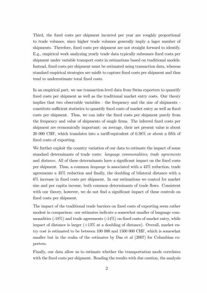
Per Firm, Good and CountryFrequency and Size of Shipments
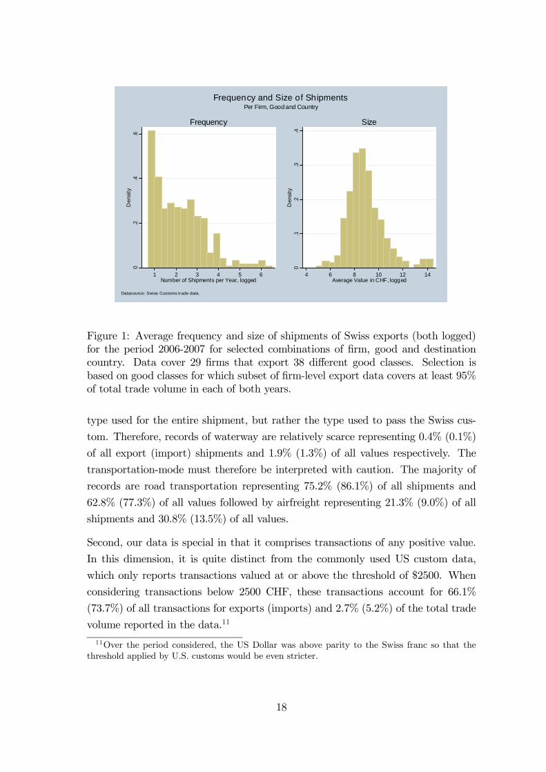
Figure 1: Average frequency and size of shipments of Swiss exports (both logged)
for the period 2006-2007 for selected combinations of firm, good and destination
country. Data cover 29 firms that export 38 different good classes. Selection is
based on good classes for which subset of firm-level export data covers at least 95%
of total trade volume in each of both years.
type used for the entire shipment, but rather the type used to pass the Swiss cus-
tom. Therefore, records of waterway are relatively scarce representing 0.4% (0.1%)
of all export (import) shipments and 1.9% (1.3%) of all values respectively. The
transportation-mode must therefore be interpreted with caution. The majority of
records are road transportation representing 75.2% (86.1%) of all shipments and
62.8% (77.3%) of all values followed by airfreight representing 21.3% (9.0%) of all
shipments and 30.8% (13.5%) of all values.
Second, our data is special in that it comprises transactions of any positive value.
In this dimension, it is quite distinct from the commonly used US custom data,
which only reports transactions valued at or above the threshold of $2500. When
considering transactions below 2500 CHF, these transactions account for 66.1%
(73.7%) of all transactions for exports (imports) and 2.7% (5.2%) of the total trade
volume reported in the data.11
11Over the period considered, the US Dollar was above parity to the Swiss franc so that the
threshold applied by U.S. customs would be even stricter.
18
4.2 Firm Level Data
Our theory is based on firm decisions and must be tested using firm level data.
Unfortunately, the universe of trade data does not include a firm identifier. How-
ever, a subset of the transaction data is collected through an electronic system that
incorporates the names of the exporting and importing firms or individuals.12 We
refer to the dataset of export as the subset of firm level data. The electronic system
was introduced in the year 2003 and is a novel tool to Swiss Customs and firms use
it on a volontary basis. Therefore, the corresponding data cover neither a constant
share of exports nor do firms which use the system necessarily report all of their
transactions through it.
For the years 2005 to 2009 covered by our data, the subset of data identifying firms
aggregate to a total of 21.8, 24.5, 40.4, 43.0, and 43.9% of total export volumes
(in CHF) for each of the five years. In order to exploit the useful information
of the subset of firm data, we identify the good categories in which "almost all"
transactions are recorded in the subset of firm level data. In particular, we focus on
good categories for which the subset reports more than 95% of total export value
within each of the years.
We exclude the year 2005 from our analysis as its includsion would limit the coverage
of firm data too severely. Moreover, we exclude observations of the years 2008 and
2009 since for these years our model’s assumption of a steady economic environment
is clearly violated.13
Overall, we deal with the years years 2006 and 2007, to which we apply the criterion
of 95% coverage described above to select firm level data of Swiss exports. Within
the thus identified subset we exclude goods that are only shipped by product unit.
As such, we eliminate the categories "motor vehicles for the transport of goods (less
than 1200 kg)" (tariff number 8704.3110) and "motor vehicles for the transport
of goods (between 1200-1600 kg)" (tariff number 8704.3120), within which each
transaction obviously represents one vehicle. Following the same reasoning, we also
eliminate the category "lamp-holders, plugs and sockets (between 0.3 and 3kg)"
(tariff number 8536.6952) and the category "articles of goldsmiths’ and silversmith’s
wares" (tariff number 7114.1990). Further, we eliminate the firms that export the
12As firm names are not standardized in the dataset provided by Swiss Customs, we need to
clean the data from different versions of spelling in order to obtain proper firm identifiers. We
restrict this process to firms for which there are at least than 24 observations.13The Baltic Dry Index, a direct measure of commodity shipping prices, fell between May 20
and December 3 2008 from 11,793 to 663 points. See http://www.bloomberg.com/.
19
51
01
5A
vera
ge
Va
lue
of S
hip
me
nt,
log
ged
0 2 4 6Number of Shipments, logged
Datasource: Swiss Customs trade data .
Average Value and Number of Shipments
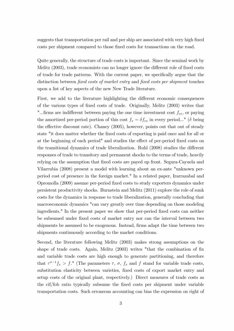
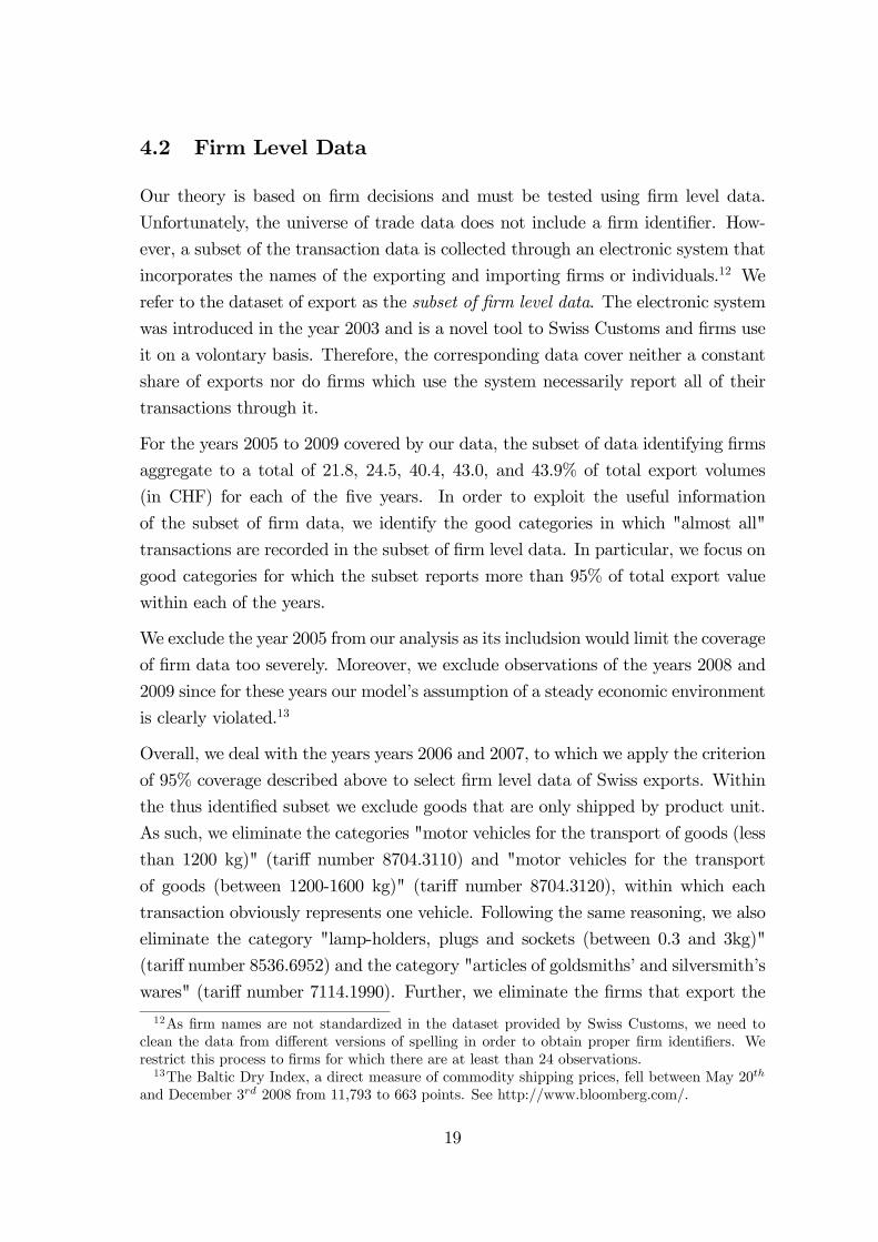
Figure 2: Scatterplot between average frequency and size of shipments (both logged)
for selected combinations of firm, good and destination country of Swiss exporters
for the period 2006-2007. See also note of Figure 1.
category "wood in chips or particles" (tariff number 4401.2200) and firms, typically
apparel exporting firms, whose transactions are in majority small shipments to
individuals. Finally, we eliminate firm-good-destination combinations with less than
two shipments per year.
Filtering the data according to the thus defined criteria leaves us with 29 firms that
export 38 different goods. Three of the firms export exactly two distinct goods and
two of which export exactly three distinct goods. These firms account for 17,211
individual transactions of a total value of 1’791’624’536 CHF.
Based on these shipments, and for each combination of firm-good-destination, we
compute the frequency (average yearly number) and the average value per shipment.
This gives us 384 observations for 62 countries. Figure 1 plots a histogram of both
variables.
Figure 2 graphs a scatterplot of these two variables. The figure shows that, in line
with the Propositions 1 and 2 above, the two margins frequency and size of shipment
tend to co-move.
20
4.3 Control Variables
The following additional data are used as control variables in the estimations below:
language commonality, a trade agreements, distance from Switzerland and GDP as
well as GDP per capita data.
World Bank WDI database provides the trade partners’ GDP as well as GDP per
capita data (both in constant US dollars). Distance, defined as distance from
Switzerland’s capital (Bern) to the trading partner’s capital, is provided by the Cen-
ter for International Prospective Studies (CEPII)14. A common language dummy is
constructed using data from the CIA World Fact Book. We set this dummy to one
if one of the official Swiss languages is an official language in a partner country as
well or if an official Swiss language is spoken by at least 25% of the population of
the respective partner country. Data on Swiss trade agreements is available from
the Swiss federal office of economics (SECO).15 Using this data we construct an
indicator function for trade agreements which is one if the agreement is in office for
at least half of a respective period of analysis.
5 Estimations
In the following empirical section we aim to use the expressions (16) and (18) to
estimated the two types of trade costs: fixed costs of shipment and fixed costs of
market entry. We ignore per period fixed costs and variable transport costs. We do
so because first, per period fixed costs are not distiguishable from market entry costs
within the static setup we focus on and, moreover, are estimated to be negligible
by existing studies (see Das et al (2007)). Second, as discussed in connection with
equation (17), we are unable to estimate variable transport with our data due to
the lack of proxies for the ideal price index and firm productivity.
All of the relevant expressions for our exercise involve the demand elasticity and the
interest rate. The former can generally be estimated (see e.g. Broda and Weinstein
(2004)) but performing such an exercise is beyond the scope of the present paper.
Instead, in our benchmark we assume the interest rate as well as the substitution
elasticity to vary within the conventional ranges ∈ [05 1] and ∈ [2 10].14French: Centre d’Etudes Prospectives et d’Information Internationale.15French: Secrétariat d’Etat à l’économie.
21
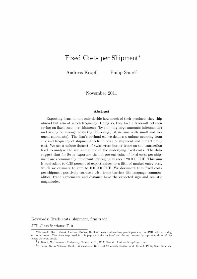
0.1
.2.3
.4D
ensi
ty
-5 0 5 10
In CHF, logged
0.5
11.
52
2.5
0 .2 .4 .6 .8 1
In Percent of Shipment Value
Datasource: Swiss Customs trade data.
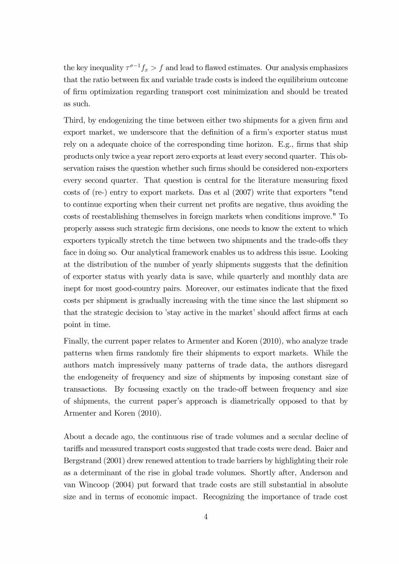
by Firm, Good and CountryImputed Fix Costs per Shipment
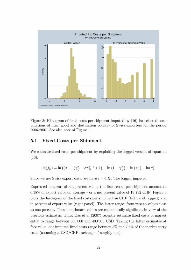
Figure 3: Histogram of fixed costs per shipment imputed by (16) for selected com-
binations of firm, good and destination country of Swiss exporters for the period
2006-2007. See also note of Figure 1.
5.1 Fixed Costs per Shipment
We estimate fixed costs per shipment by exploiting the logged version of equation
(16):
ln() = ln¡( − 1) − −1 + 1
¢− ln ¡1− ¢+ ln ()− ln()
Since we use Swiss export data, we have = . The logged imputed
Expressed in terms of net present value, the fixed costs per shipment amount to
0.38% of export value on average — or a net present value of 19 792 CHF. Figure 3
plots the histogram of the fixed costs per shipment in CHF (left panel, logged) and
in percent of export value (right panel). The latter ranges from zero to values close
to one percent. These benchmark values are economically significant in view of the
previous estimates. Thus, Das et al (2007) recently estimate fixed costs of market
entry to range between 300’000 and 400’000 USD. Taking the latter estimates at
face value, our imputed fixed costs range between 5% and 7.5% of the market entry
costs (assuming a USD/CHF exchange of roughly one).
22
We aim to extract the determinants and drivers of the fixed costs per shipment.
Specifically, we formulate an empirical model as
ln() = + +X
∈ +
where matrix stands for a set of economic variables, which we can reasonably
suspect to impact fixed costs of shipments: dummies for common language, bilat-
eral trade agreements as well as distance; dummies for the transportation modes,
i.e. railway, air and mail. Further, are dummies of our good category, which we
include to capture good-specific effects like the durability of goods, e.g. affecting
storage costs. Finally is a measurement error, assumed to be normally distrib-
uted. We perform OLS estimations with clustered error estimation to correct for
heteroskedasticity bias.
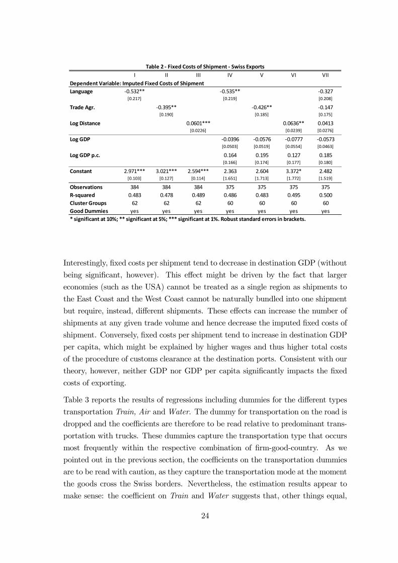
Table 2 reports our estimates. Columns I - III present the results for specifica-
tions where the variables Common Language, Trade Agreement and Distance of
the destination country from Switzerland (measured in km between capitals and
logged) enter separately in the regression. All three coefficients are significant at
the 5 percent level and have the expected sign: while setup cost tends to decrease
with language commonalities and under trade agreements, it increases in distance.
Columns IV - VI shows that these results remain largely unchanged when control-
ling for GDP and per capita GDP of the destination country (both logged). The
estimations suggests that the effect of a common official language is huge, implying
a reduction of fixed costs per shipment of about 43% (exp(−535)1 ≈ 0586). Sim-ilarly, the establishment of a trade agreement would imply a reduction of this type
of costs of about 35% (exp(−426)1 ≈ 0653); and finally, a doubling of bilateraldistance increases the respective shipment costs by about 6%.16
16Here and in the following regressions, the estimated coefficients remain largely unchanged in
terms of magnitude when changing the demand elasticity and interest rate in the ranges [2,10] and
[0.05,0.1]. Signs and significance levels are unaffected.
23
I II III IV V VI VII
Language ‐0.532** ‐0.535** ‐0.327[0.217] [0.219] [0.208]
Trade Agr. ‐0.395** ‐0.426** ‐0.147[0.190] [0.185] [0.175]
Log Distance 0.0601*** 0.0636** 0.0413[0.0226] [0.0239] [0.0276]
Log GDP ‐0.0396 ‐0.0576 ‐0.0777 ‐0.0573[0.0503] [0.0519] [0.0554] [0.0463]
Log GDP p.c. 0.164 0.195 0.127 0.185[0.166] [0.174] [0.177] [0.180]
Constant 2.971*** 3.021*** 2.594*** 2.363 2.604 3.372* 2.482[0.103] [0.127] [0.114] [1.651] [1.713] [1.772] [1.519]
Observations 384 384 384 375 375 375 375
R‐squared 0.483 0.478 0.489 0.486 0.483 0.495 0.500
Cluster Groups 62 62 62 60 60 60 60
Good Dummies yes yes yes yes yes yes yes
Table 2 ‐ Fixed Costs of Shipment ‐ Swiss Exports
Dependent Variable: Imputed Fixed Costs of Shipment
* significant at 10%; ** significant at 5%; *** significant at 1%. Robust standard errors in brackets.
Interestingly, fixed costs per shipment tend to decrease in destination GDP (without
being significant, however). This effect might be driven by the fact that larger
economies (such as the USA) cannot be treated as a single region as shipments to
the East Coast and the West Coast cannot be naturally bundled into one shipment
but require, instead, different shipments. These effects can increase the number of
shipments at any given trade volume and hence decrease the imputed fixed costs of
shipment. Conversely, fixed costs per shipment tend to increase in destination GDP
per capita, which might be explained by higher wages and thus higher total costs
of the procedure of customs clearance at the destination ports. Consistent with our
theory, however, neither GDP nor GDP per capita significantly impacts the fixed
costs of exporting.
Table 3 reports the results of regressions including dummies for the different types
transportation Train, Air andWater. The dummy for transportation on the road is
dropped and the coefficients are therefore to be read relative to predominant trans-
portation with trucks. These dummies capture the transportation type that occurs
most frequently within the respective combination of firm-good-country. As we
pointed out in the previous section, the coefficients on the transportation dummies
are to be read with caution, as they capture the transportation mode at the moment
the goods cross the Swiss borders. Nevertheless, the estimation results appear to
make sense: the coefficient on Train and Water suggests that, other things equal,
24
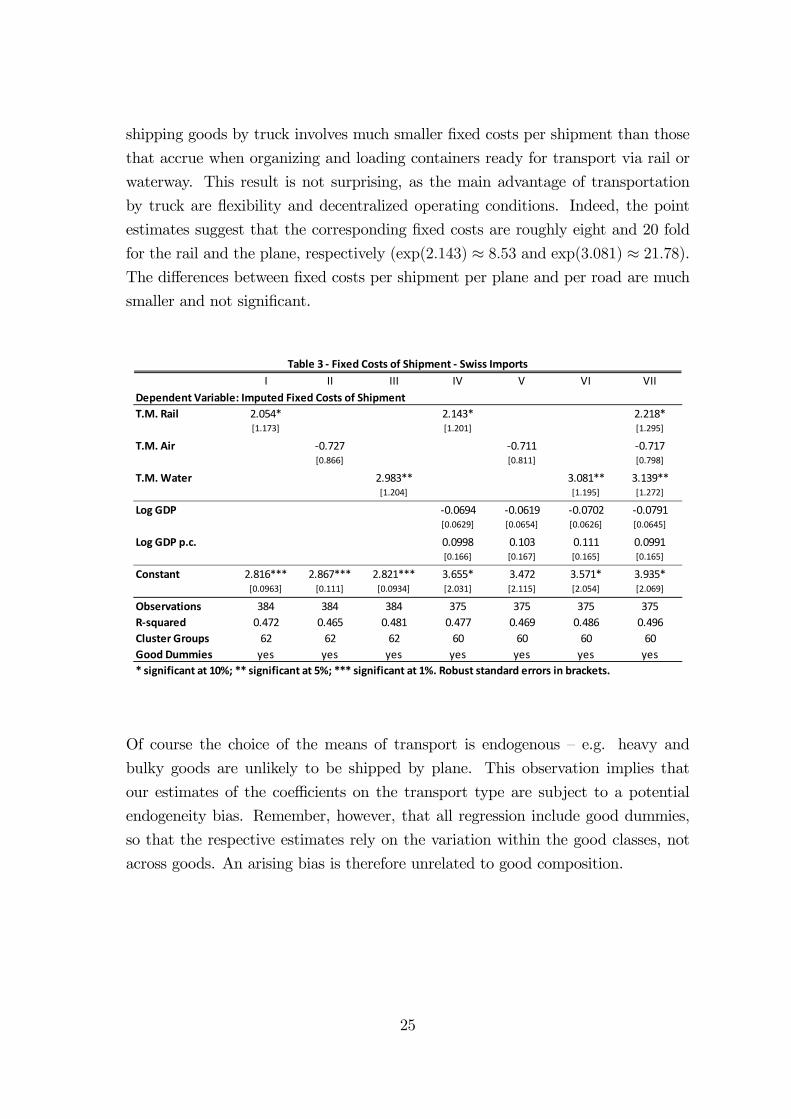
shipping goods by truck involves much smaller fixed costs per shipment than those
that accrue when organizing and loading containers ready for transport via rail or
waterway. This result is not surprising, as the main advantage of transportation
by truck are flexibility and decentralized operating conditions. Indeed, the point
estimates suggest that the corresponding fixed costs are roughly eight and 20 fold
for the rail and the plane, respectively (exp(2143) ≈ 853 and exp(3081) ≈ 2178).The differences between fixed costs per shipment per plane and per road are much
smaller and not significant.
I II III IV V VI VII
T.M. Rail 2.054* 2.143* 2.218*[1.173] [1.201] [1.295]
T.M. Air ‐0.727 ‐0.711 ‐0.717[0.866] [0.811] [0.798]
T.M. Water 2.983** 3.081** 3.139**[1.204] [1.195] [1.272]
Log GDP ‐0.0694 ‐0.0619 ‐0.0702 ‐0.0791[0.0629] [0.0654] [0.0626] [0.0645]
Log GDP p.c. 0.0998 0.103 0.111 0.0991[0.166] [0.167] [0.165] [0.165]
Constant 2.816*** 2.867*** 2.821*** 3.655* 3.472 3.571* 3.935*[0.0963] [0.111] [0.0934] [2.031] [2.115] [2.054] [2.069]
Observations 384 384 384 375 375 375 375
R‐squared 0.472 0.465 0.481 0.477 0.469 0.486 0.496
Cluster Groups 62 62 62 60 60 60 60
Good Dummies yes yes yes yes yes yes yes
* significant at 10%; ** significant at 5%; *** significant at 1%. Robust standard errors in brackets.
Table 3 ‐ Fixed Costs of Shipment ‐ Swiss Imports
Dependent Variable: Imputed Fixed Costs of Shipment
Of course the choice of the means of transport is endogenous — e.g. heavy and
bulky goods are unlikely to be shipped by plane. This observation implies that
our estimates of the coefficients on the transport type are subject to a potential
endogeneity bias. Remember, however, that all regression include good dummies,
so that the respective estimates rely on the variation within the good classes, not
across goods. An arising bias is therefore unrelated to good composition.
25
5.2 Market Entry Costs
We now turn to the analysis of the entry costs to export markets. To this aim, we
use condition (18), which binds for the marginal exporter
ln() = ( − 1)∆ + ln ()− ln(1− ) (19)
When we proxy the fixed costs of market entry with the minimum of the expression
of the right, our firm date are far too few observations to provide a reasonable
upper bound. To circumvent this lack of data we use to the full trade data set
without firm identifiers under one assumption. Specifically, we assume that, within
each broad sector and for each good-country pair, the good that is least exported
(generating the lowest observation for the right had expression in (19)) there is only
one exporter.
Under this assumption, we can, at the cut-off, identify the good with one firm and
calculate the right hand side using our full set of trade data. In particular, the
minimum value of the right hand side of (19), calculated by identifying goods with
firms, constitutes a proxy for the left hand side.
We do not only exploit the country dimension, but also the dimension of sectors,
which we define by the two-digit level of out tariff number. There are 95 sectors
and 5778 country-sector pairs for export and 3676 corresponding pairs for import
data. Since the number of exported goods per trade partner is generally larger than
the number of imported goods per trade partner, there are less observations on the
good-sector level for import data. Finally, keep excluding the years of the financial
crises and the Great Trade Collapse (2008 and 2009) but include the first year of
our dataset 2005, which was previously dropped due to scarcity of firm level data.
We compute the right hand side in (19) for the standard values = 5 and = 05.
To eliminate potential bias through outliers in the observations of our proxy (19),
we also take averages over the two and three smallest observations, respectively.
This change of definition does not alter our qualitative results.
The average of our proxies of market entry cost is 98 270 CHF for exports and
149 711 CHF for imports. These estimates are considerably lower than the ones
estimated in Das et al (2007), which range between 300 000 and 400 000 USD for
Colombian exporters. Nevertheless, our proxies range within the same order of
26
magnitude.17 Moreover, Das et al (2007) infer entry costs of exporters and non-
exporters and, indeed, write that "entrants tend to get favorable entry cost draws,
so average entry costs incurred are considerably lower." Since we base our estimate
on active exporters only, this effect may explain part of the difference between our
results and those in Das et al (2007). A further potential explanation may be
based of Swiss efficiency of exporting procedures, which may be characteristic for
an economy that is paradigmatic for a small open economy.
17When defining market entry costs over the lowest two or three observations, our estimates
reach 145651 (222195) and 185109 (282438) for imports (exports).
27
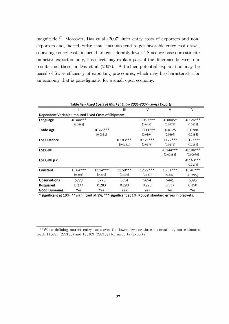
Based on our proxies for market entry costs, we repeat the estimations reported in
Tables 2 and 3, which were conducted for fixed costs per shipment. Doing so, we
can now rely on export and import data, since we are not using firm level data.
Table 4a reports the regression results of our proxy of on the dummy variables
Common Language, Trade Agreement, and Distance from our previous estimates
for our export data. Columns I - IV represent our standard specifications; the fixed
costs are proxied with the lowest values of (19) separately for each export market.
The estimates of the coefficients on Common Language and Trade Agreement are
statistically significant with the expected negative sign, tough considerably smaller
than those of the regressions of the fixed costs per shipment in Table 2. Also the
impact of Distance is significant in the specifications of Column III and IV.
To eliminate the potential influence of market size, we Columns V and VI succes-
sively include the destination GDP and the destination GDP per capita (both in
logs). As in the regression with fixed costs per shipment, the estimated coefficients
on Trade Agreement are lower now cease to be significant.
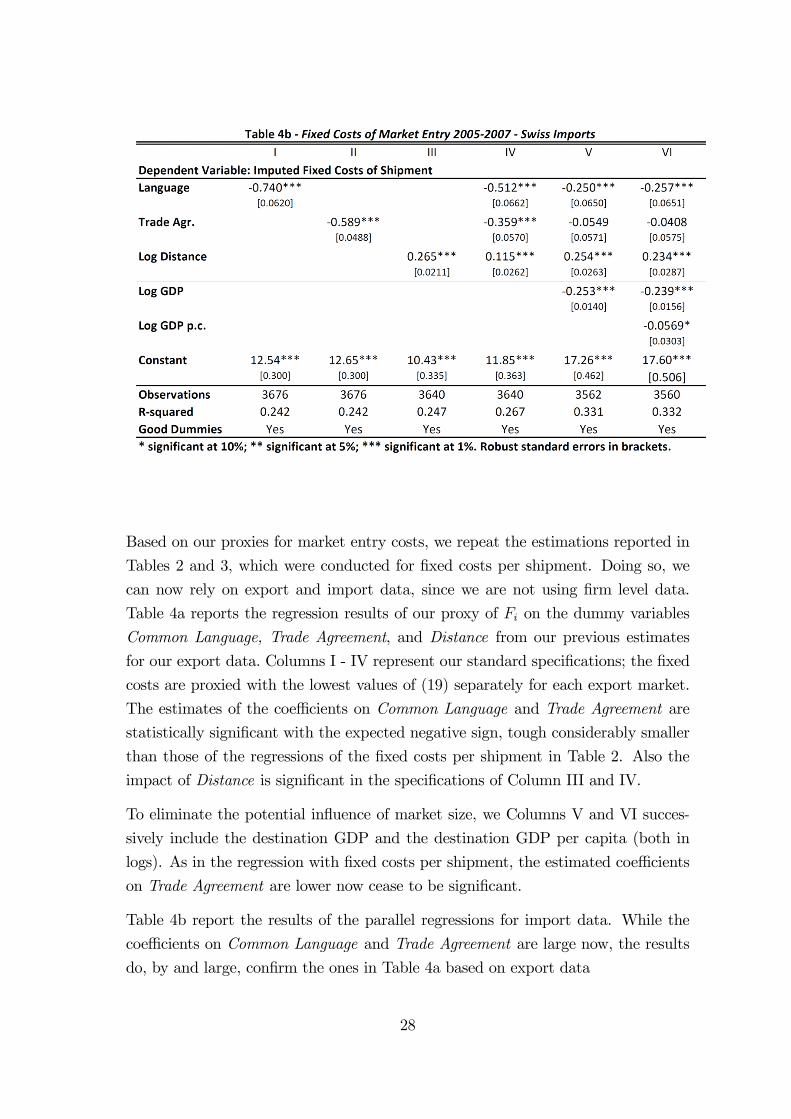
Table 4b report the results of the parallel regressions for import data. While the
coefficients on Common Language and Trade Agreement are large now, the results
do, by and large, confirm the ones in Table 4a based on export data
28
5.3 Discussing Both Types of Fixed Costs
Having estimated fixed costs per shipment and market entry costs, we can compute
the net present value of the former as a ratio of the latter. This ratio indicates that
the total value of fixed costs per shipment is roughly a fifth of the value of mar-
ket entry costs (1979298270 ≈ 02014). This number is economically significant,particularly so in comparison with previous estimates of per period fixed costs of
exporting. Thus, referring to per period fixed costs, Das et al (2007) write that
"these costs, on average, are negligible." By comparison, our estimates of the fixed
costs per shipment are very large. Too large, in any case to be ignored in trade
models that react sensitively to the shape and size of trade costs.
When fixed costs per shipment are large, the natural question arises why they do
not proxied by per period fixed costs, thus entering standard estimates of the latter.
Indeed, as an ommitted variabel fixed costs per shipment could be expected to
induce an upward bias of per period fixed costs. The obvious reason why such a
bias is unlikely is the fact that fixed costs per shipment rise roughly proportinately
with export volumes and therefore tend to be subsumed in variable costs in standard
estimations. In sum, when properly accounting for fixed costs per shipment, the
estimated size of variable transport costs is likely to be reduced.
Introducing fixed costs per shipment and endogenizing the period between two ex-
port transactions also raises the question whether there are scale or learning effects
that reduce fixed costs over time (as Segura-Cayuela and Vilarrubia (2008) regard-
ing per period fixed costs). In such a setting, shipments could occur more frequently
to reap the benefits of learning. Conversely, shipping goods too infrequently could
be suboptimal as such a strategy would raise the overall trade costs. These con-
siderations also direct the attention to parallel questions regarding fixed costs of
market entry. Thus, Das et al (2007) find that maintain their exporter status under
adverse market conditions to avoid "the costs of reestablishing themselves in foreign
markets when conditions improve." Once we think about endogenous frequency, we
may wonder about the definition of reentry. Does the full amount of market entry
costs accrue when a firm reenters a market it did not supply for six one, two or
five year? Given that these reentry costs are continuous in time of absence, they
would surely impact the firms’ optimal strategy concerning size and frequency of
shipments.
29

6 Conclusion
This paper has analyzed the role, size and determinants of fixed costs per shipment.
Out theory rests on the assumption that exporting firms optimally trade off the fixed
costs of exporting and storage costs at export markets. Conceptually, we have shown
that fixed costs per shipment introduce a new margin along which trade volumes
expand and contract. Further, being substitutable with storage costs, they smear
the border between fix and variable costs of trade. Moreover, we have presented a
method to infer different types of trade costs — fixed costs per shipment, variable
transport costs and fixed costs of market entry — from cross-border trade data on the
transaction level. This methodology enables us to disentangle and analyze the two
types of fixed costs of exporting, using disaggregated Swiss export and import data.
Our findings suggest that fixed costs per shipment are economically significant and
considerably larger than the per-period fixed costs estimated in earlier studies. In
particular, our estimates of the net present values of fixed costs per shipment are
around 20 percent of fixed costs of market entry.
30
A Appendix
A.1 Proofs
Proof of (11) According to the concept of iceberg costs, the value of goods boarded
for shipment consists of the product consumed quantity and . Thus,
=
Z ∆
0
( 0)0 =
∙
− 1
¸1−1−
=
¡1−
¢
Proof of (12)
ln () =1
− −1
1−
2
1
( − 1)−2
¡1−
¢=
1
1
( − 1) ¡1− ¢ ¡1−
¢ µ( − 1) ¡1− ¢ ¡1−
¢−
¶=
1
− 1 + −
( − 1) ¡1− ¢ ¡1−
¢(Used (10) in the last step.)
Proof of (13) Use (9) to check
=1
1−
½
1−
−
¾=
1
1−
©1− −
ª=
−1
where the last step follows from (10).
Proof of (14) Rewrite (10) as
−1
£( − 1) −
¤=
− 1
Using (18), this implies
− 1∙1 +
−
¸−1=
Given that the cutoff productivity is unique, this equation implies that be
constant if fixed costs of exporting and are constant. Hence, (18) implies (8).
31
A.2 References
Anderson J. and van Wincoop E. 2003: "Gravity With Gravitas: A Solution to the
Border Puzzle" American Economic Review, Vol. 93, No. 1, pp. 170-192
Anderson J. and van Wincoop E. 2004: "Trade Costs" Journal of Economic Liter-
ature, Vol. 42, No. 3, pp. 691-751
Anderson, James E. and Yoto V. Yotov 2008: “The Changing Incidence of Geogra-
phy,” American Economic Review, Vol. 100 pp. 2157—2186
Armenter, Roc and Miklos Koren 2010: “A Bins-and Balls Model of Trade,” mimeo
CEU
Bernard, Andrew B., J. Bradford Jensen and Peter K. Schott 2003: "Plants and
Productivity in International Trade," American Economic Review, Vol. 93 (4), pp.
1268-1290
Bernard, Andrew B., J. Bradford Jensen and Peter K. Schott 2006: "Trade costs,
firms and productivity ," Journal of Monetary Economics, Vol. 53 (5), pp. 917-937
Bernard, Andrew B., J. Bradford Jensen, and Peter K. Schott. (forthcoming.)
“Importers, Exporters and Multinationals: A Portrait of Firms in the U.S. that
Trade Goods.” In Producer Dynamics: New Evidence from Micro Data, ed. T.
Dunne, J. B. Jensen, and M. J. Roberts. University of Chicago Press.
Bernard, Andrew B., J. Bradford Jensen, Stephen J. Redding, and Peter K. Schott
2007: "Firms in International Trade," Journal of Economic Perspectives, Vol. 21
(3), pp. 105—130
Burstein, Ariel and Marc J. Melitz 2011: "Trade Liberalization and Firm Dynam-
ics," NBER WP 16960
Chaney, Thomas 2005: "The Dynamic Impact of Trade Opening: Productivity
Overshooting with Heterogeneous Firms," mimeo University of Chicago
Crozet, Matthieu and Pamina Koenig 2010: "Structural gravity equations with
intensive and extensive margins," Canadian Journal of Economics, Vol. 43, No. 1
32
Das, Sanghamitra; Mark J. Roberts and James R. Tybout: 2007: "Market Entry
Costs, Producer Heterogeneity, and Export Dynamics" Econometrica, Vol. 75 (3),
pp. 837-873
Helpman, E., M. Melitz, and Y. Rubinstein 2008: “Estimating Trade Flows: Trading
Partners and Trading Volumes,” Quarterly Journal of Economics, Vol. 123, pp.
441-487
Hummels, David (1999), “Have International Transportation Costs Declined?” mimeo,
Purdue University.
Irarrazabal, Alfonso and Luca David Opromolla 2009: "The Cross Sectional Dy-
namics of Heterogenous Trade Models," mimeo, Banco de Portugal
Jacks, David S. and Meissner, Christopher M. and Novy, Dennis 2008: "Trade costs,
1870—2000," American Economic Review, Vol. 98 (2), pp. 529-534
McCallum, J. 1995: "National Borders Matter: Canada-U.S. Regional Trade Pat-
terns," American Economic Review, Vol. 85, No. 3, pp. 615-623.
Melitz, Marc J. 2003: “The Impact of Trade on Intra-industry Reallocations and
Aggregate Industry Productivity,” Econometrica, 71 , pp. 1695—1725.
Novy Dennis 2011: “Trade Booms, Trade Busts and Trade Costs.” Journal of In-
ternational Economics 83(2), pp. 185-201.
Roberts, Mark J. and James R. Tybout1997: “The Decision to Export in Colombia:
An Empirical Model of Entry with Sunk Cost,” American Economic Review, Vol.
87, pp. 545—564.
Ruhl, Kim 2008: "The International Elasticity Puzzle," mimeo, NYU Stern School
of Business
Segura-Cayuela, Rubén and Josep Vilarrubia 2008: “Uncertainty and entry into
export markets” Banco de España Working Papers - No. 0811
33