Embed Size (px)
Citation preview
Acce
pted
Integration of Open Source Tools for Studying Large-ScaleDistribution Networks
G Valverde1 A Arguello1 R Gonzalez1 J Quiros-Tortos1
1Electric Power and Energy Research Laboratory University of Costa Ricagustavovalverdeucraccr
Abstract The penetration of Low Carbon Technologies (LCTs) is expected to increase in thenear future given the attractive incentives from governments the cost-effectiveness of the tech-nologies and the appearance of Smart Grid schemes To understand the corresponding benefitsand challenges associated with them power utilities are expected to run more sophisticated studiessupported by more accurate and detailed models of distribution network elements and the networkitself This paper presents the development of two software plugins that allow the integration ofa Geographical Information System (GIS) platform with a distribution system simulator Theseplugins are intended to provide power utilities free and open source tools to explore the benefitsandor impacts of newly adopted LCTs and to analyze Smart Grid opportunities in large-scaledistribution networks The effectiveness of the plugins is illustrated considering a real DN with13323 customers in Costa Rica Results demonstrate that the plugins can successfully support inthe creation of detailed network models and studies
1 Introduction
Planning studies for distribution networks have been fulfilled with the assistance of engineeringnetwork models and simulation tools that have helped understanding the network behavior underparticular conditions At present most distribution system analysis tools are capable of runningunbalanced three phase power flows and short circuit analysis while only a few tools have thecapability to perform simulations over a period of time such as day week month or year [1]
Modeling of the distribution network generally ignores the secondary distribution system Hencethe analysis is usually limited to Medium Voltage (MV) level with distribution transformers re-placed by aggregated loads These simplifications were acceptable because Low Voltage (LV)systems have been considered passive while modeling these secondary systems is not trivial
The increasing integration of Low Carbon Technologies (LCTs) such as Distributed EnergyResources (DER) and the implementation of Smart Grid schemes at the distribution level bringsnew modeling requirements in which secondary LV lines and distribution transformers can nolonger be neglected but need to be modeled in detail As thoroughly discussed in [2] modelingsecondary is not easy and it will take time and effort to accomplish Having said that as computerresources grow in power and capability it is just a matter of time before all successful utilities havemade this important step
Fortunately most of the information required to model LV elements is readily available in theGeographical Information Systems (GIS) of power utilities [3] hence processing of this GIS data ismandatory Indeed GIS provides the needed data management analysis and awareness to help the
1
Acce
pted
smart grid really be smart [4] Reference [2] outlines the data recommendations and requirementswhen performing analyses on secondary systems In addition [5] reports on a database of typicalDistribution Network (DN) element parameters to be used as a complement for GIS data
References [3] and [6] report on the creation of hundreds of LV network models from GIS datain UK In both cases the files were exported to Matlab for the data processing and creation of theengineering network models in the corresponding power system simulation tool However anychange in the GIS data would require a new iteration of data (files) exchange among pieces ofsoftware which may be time consuming and even tedious when dealing with long DN feeders andhundreds of secondary systems Hence the use of power system tools directly fed from GIS wouldprovide great opportunities for easier handling of simulations [7]
At present time there are many software tools to carry out distribution network studies Al-though commercial software are well tested and computationally efficient they do not allow chang-ing the code for adding new algorithms [8] not to mention the license and update costs Hencethe Electric Power Research Institute (EPRI) and the US Pacific Northwest National Laboratorydeveloped and released the OpenDSS and the GridLab-D respectively Two sophisticated opensource software tools for the future smart grid studies [9] [10]
An important drawback of these powerful tools is the fact that they do not make direct use ofGIS This is although they may use the information from GIS as input parameters these simulatorsdo not interact with the GIS of the power utility
This paper presents the integration of OpenDSS with an open source GIS platform QuantumGIS (QGIS) to carry out easier and more efficient studies of distribution networks The integrationis made possible with the creation of software plugins to a) extract GIS data to automaticallybuild a DN engineering model and b) run OpenDSS as an embedded tool in the GIS platformThis integration is a great opportunity to keep an updated and accurate GIS representation of thenetwork It is expected that a Graphical User Interface (GUI) for OpenDSS will further enhancethe acceptability of OpenDSS and this opens an opportunity to power utilities and researchersto run their smart grid studies at minimum cost The plugins will help on planning studies (loadgrowth network extension DER integration) but they could also help on operating proceduresif some decisions required lsquoon-linersquo simulations In order to provide new opportunities to powerutilities research laboratories and universities to test and simulate novel smart grid solutions theplugins have been made available in [11]
The remaining of this paper is organized as follows Section 2 gives a brief description ofOpenDSS and the QGIS and how they are integrated Section 3 presents a detailed explanationof the network model builder using GIS data while Section 4 presents the type of DN studies thatcan be carried out in the GIS environment Furthermore a demonstration of two network studiesis presented in Section 5 followed by a discussion in Section 6 of future complementary tools thatwill take more advantages of GIS from a smart grid perspective Finally Section 7 presents theconcluding remarks
2 Integration of Free and Open Source Platforms
In the last decade open source and free software have become more and more popular in thescientific and engineering community They have the advantage of flexibility ie users can adjustthe code and customize the tools according to particular needs In addition they offer universalaccessibility to technological advances and make it possible to accelerate software capabilities asuser feedback and contributions are regularly incorporated Indeed open source software tools
2
Acce
pted
have demonstrated to foster further developments ideas and innovation In the case of powersystem analysis reference [12] provides a list of available open source software tool for a varietyof transmission and distribution network studies This paper reports on enhanced simulation toolsfor smart grid studies thanks to the integration and combination of OpenDSS and QGIS Bothsoftware are briefly explained hereafter
21 OpenDSS
OpenDSS is an open source software package developed by EPRI that can be used to simulatemulti-phase AC distribution networks [9] for planning and network analysis It was developed tosupport the grid modernization efforts and the integration of DER
A key aspect of this script-driven frequency-domain simulation tool is that it allows consideringthe time dimension (eg daily simulations with different time step) - critical to quantifying theimpacts of variable sources and loads According to EPRI the tool was designed to be indefinitelyexpandable so that it can be easily modified to meet future needs and smart grid studies
To create a network model OpenDSS follows a sequence of definitions [9] for each networkelement ie generators lines transformers and loads Hence given the script-written nature ofthis software the creation of large-scale networks must be done carefully and hopefully in anautomated way
According to EPRI the software was designed with the recognition that developers would neverbe able to anticipate what future users will do with it Hence a Component Object Model (COM)interface was implemented on the in-process server DLL version of the program This COM serverallows users to integrate OpenDSS with other software packages or programming languages (egExcel with VBA Matlab Python) to perform more sophisticated studies This COM server is thekey feature to integrate OpenDSS and QGIS as explained in Section 4
22 QGIS
GIS are computer based systems used by many service utilities and government institutions tostore read edit and analyze data referenced by a spatial coordinate system [13]
GIS allow a graphic representation of data For example power utilities use GIS to store charac-teristics and attributes of utility assets such as electric poles lines transformers and final customerelectric meters all of them geo-referenced by a coordinate system that allows to find their exactlocation The object location is the common attribute among GIS elements This information isdefined according to the appropriate coordinate and projection system
One of the most popular open source tools for geographical systems is Quantum GIS or simplyQGIS under the GNU-GPL license This free software reads and analyzes shp files (compatiblewith commercial software) of GIS layers which contain information of object classes eg layerof MV lines layer of MVLV transformers etc
An important feature of QGIS is that it offers the possibility to develop Python written pluginsfor extra data processing and analysis not available in the existing software [14] This is the keyfeature to integrate QGIS and OpenDSS as reported in Sections 3 and 4
3 Engineering DN Model Builder
The first tool reported in this paper is called QGIS2OpenDSS It was developed to extract andprocess GIS data of DN elements to generate the OpenDSS files in an automated way As presented
3
Acce
pted
in Fig 1 this plugin makes use of a GUI that allows the user to select the opened GIS layers to betranslated into OpenDSS files Note that users must define a short name that is later used to defineall buses and line segments Additionally the user must define the path where the loadshapes arelocated and the desired location of the resulting OpenDSS files
The tool accepts up to three layers of MV lines distribution transformers LV secondary linesLV services LV loads and a single substation layer It is very common to find separate files foroverhead lines and underground cables For underground cables the user will have to tick the UGoption shown in Fig 1
Figure 1 Graphical User Interface for QGIS2OpenDSS
31 Data Requirements
This plugin has the following data requirements
bull HVMV Substation This layer is optional and should be used when the main power trans-former is to be modeled along with the feeder A single-point layer details the number ofwindings impedances nominal voltages kVA ratings number of taps and the short circuitcapacity at HV level
bull MV Lines The attributes to be found in this layer are the number of phases of the linesegment and its identification ie abc for three phase segments ab bc or ca for two phasebranches and a b or c for single phase laterals Additionally information of neutral andphase conductors such as length material and conductor size is later used to get the electricalproperties of each conductor in a wire database [5] The size can be given in Millions ofCircular Mils (MCM) American Wire Gauge (AWG) or mm2 as all attributes are treated asstringsFor overhead lines the table of attributes must include a line spacing code or letter egV may refer to vertical line spacing and H for horizontal spacing and so on The plugin
4
Acce
pted
concatenates strings to build a unique OpenDSS line geometry identifier [15] For examplethe identifier 3PMV 477AAC30AAC H stands for a three phase MV line in horizontalspacing whose phase conductors are 477 MCM AAC and neutral conductor 30 AWGAACUnderground line segments must also include the insulating material nominal voltage andcable type (concentric neutral or tape shielded cables) This information is used to extract theelectrical properties and dimensions of cables from a database for details see [5]
bull Distribution Transformers This layer must include the transformerrsquos nominal voltages andcapacity in kVA For transformer banks each unit must be specified with a given kVA ca-pacity Similar to MV lines it must include the number and identification of phases eachtransformer is connected to on the MV (primary) side In the case of three phase transformersit is imperative to include the winding connection (wye delta open wye open delta)The series impedance and no-load losses of distribution transformers are normally not in-cluded in GIS In order to create an OpenDSS model the plugin uses a database of typicalseries impedances based on the nominal voltage and capacity of transformers see [5] Forsingle phase three winding transformers an approximation is made to calculate each windingimpedance based on the transformerrsquos nameplate impedance as explained in [16] and [17]
bull LV lines Apart from the length material and size of neutral and phase conductors thislayer must include the conductor spacing the number of phases and the operating voltagecode to discriminate single phase three wire (split phase 120240 V) from three phase lines(eg 120208 V or 277480 V) For underground LV cables the attributes must include theinsulation type and cable spacing code
bull LV Wire Services The LV wire service layer must include the length type size and ma-terial of conductors These strings are concatenaded to define the linecode identifier inOpenDSS [15] For example the linecode identifier TRPX2AAC stands for a 2 AWG AACTriplex cable This identifier is later used to consult a database of electrical and mechanicalparameters of service cables to calculate their corresponding primitive impedance matricessee [5]
bull LV Loads This layer must include the average monthly kWh consumption and customertype residential commercial or industrial in order to allocate load profiles as explained inSection 34
Standardized GIS models are vital to make it possible the translation to engineering modelsTo the authorsrsquo knowledge most power utilities use very similar procedures to represent networkelements and store their information in GIS databases In case that some information is not foundin the list of attributes an error message will warn the user that some attributes are missing Thismessage may also appear if the GIS layers use attribute names not recognized by the tool Thisis easily overcome by changing the corresponding names in the table of attributes as requested byQGIS2OpenDSS
32 Connectivity of Elements
The QGIS2OpenDSS connects two or more elements if their coordinates match or when they arecloser than a predefined distance This is accomplished with Kd-trees A Kd-tree is a data structureused to organize and manipulate spatial data [18] This structure allows to quickly find neighbor
5
Acce
pted
points within a radius of a query point The spatialKDTree sub-package was used to grow thetrees in Python Also the following sub-packages were used
bull treequery pairs(r) it finds all pairs of points within a distance r in the tree This was usedto connect same class elements eg three phase MV lines
bull treeAquery ball tree(treeB r) it finds all pairs of points from tree A and tree B whosedistance is at most r This was used to connect different class elements eg three phase andsingle phase MV lines
For all cases r = 01 m This distance is used to guarantee that small errors in coordinates willnot lead to disconnected DN elements
In order to connect MV lines the tool builds a tree for each MV line type single phase twoand three phases A bus name is created when two line segments ends are found to be connectedusing the aforementioned packages In case that one of the segment ends is already assigned witha bus name the other line segment end will adopt it For example the MV bus of transformersadopt the bus name of the MV line segment end they are connected to In addition the secondarybuses of these transformers are assigned with a new LV bus name
Similarly in order to find the connectivity of LV elements the tool builds trees for LV linesegment coordinates (both ends) service coordinates (both ends) and load coordinates Here allLV elements are compared against each other to define all the LV buses
33 Identification of Errors
The information contained in GIS is very detailed However it contains errors that may remainunseen unless a network model needs to be built for engineering analysis This tool identifies andreports the errors that will affect the simulations in OpenDSS This report includes the name andcoordinates of the problematic elements to facilitate the corresponding correction in the databaseAfter all corrections are carried out the plugin should be re-run until no errors are reported
The most common error in GIS is the disconnection of DN elements due to small coordinatemismatches in the order of a few centimeters If any DN element is identified (with Kd minus tree)not connected to any other element the plugin will report it as an isolated element
The tool also checks for erroneous phase designations of MV lines in GIS The first check ismade when two phase line segments are connected For example a bc line segment should neverbe connected to an ab or ca segment otherwise an error will be reported
The next check is made when single phase segments are connected to two phase line segmentsFor example an error is reported if a phase c line segment is connected to an ab line segment Thesame procedure is repeated when connecting single phase segments only The plugin reports errorswhen connecting ararr b brarr c or crarr a segments
Similarly errors are reported when three phase transformers are connected to two phase orsingle phase lines when two phase transformers are connected to single phase segment ends orwhen the phase identification of a single phase transformer does not match the phase identificationof a single phase MV line Finally the plugin also reports unknown capacities or unknown nominalvoltages of distribution transformers They are considered unknown values when they are notincluded in the library of transformer impedances
6
Acce
pted
34 Load Profile Allocation
QGIS2OpenDSS allocates a load profile to each customer based on the customer type and monthlyenergy consumption The curves must be loaded by the user as shown in Fig 1 These curves arescaled up or down to perfectly match the customerrsquos monthly energy consumption These curvesare later fine tuned in the load allocation procedure to match the OpenDSS simulation with thefeederrsquos load profile as explained in Section 42
The load profiles are created with a resolution of 10 minutes considering different power utili-ties type of day (weekdayweekend) and energy consumption range These profiles were extractedfrom a statistical analysis of a nationwide measurement campaign in Costa Rica [19] These loadprofiles are constantly improved as more measurements become available It is expected that loadprofiles from smart meters will replace the ones obtained from the measurement campaign to assessthe benefits and impacts of integrating LCTs into the grid [4]
4 Network Analyzer
The second tool reported in this paper is the QGIS2runOpenDSS This plugin uses the outputfiles of QGIS2OpenDSS and runs the power system analyzer OpenDSS as an embedded toolin QGIS This is made possible thanks to the COM server that links OpenDSS with Python (seeSection 41)
Fig 2 presents the GUI in QGIS used to carry out advanced studies for large-scale distributionnetworks The user must select the name of the circuit created by QGIS2OpenDSS in Choosethe circuit The corresponding folder will include a masterdss file which calls the complementaryfiles of lines transformers and so on The substationdss file if created is used to automaticallyload the source voltage angle and frequency the short circuit capacities and the name of the firstMV bus connected to the main transformer
The user also has to select the feederrsquos load shape of active and reactive power along with therespective hour and date In order to run yearly power flows the file must include at least one yearof measurements This information is registered at substation level and stored in a single csv fileto carry out the load allocation procedure explained in Section 42
The user must define the type of study to be carried out and the folder where the results will bestored For snapshot studies it is required to define the simulation date and hour (available in thefeederrsquos load shape file) while yearly power flows require the simulation resolution (eg 1 min10 min 60 min etc) The user may also choose to run multiple snapshot or daily simulations if aMonte Carlo approach is to be adopted
41 Integration of QGIS and OpenDSS
QGIS drives OpenDSS via the Python console available in the former The library comtypespyis used for this purpose and this is installed using the package management system pip Thefollowing steps are required for this integration
bull Open the OSGeo4WShell (the command window of QGIS) as administrator
bull Change the path to find the file lsquoget-pippyrsquo which should have been previously downloadedThis is done using the lsquocdrsquo command
bull Install the package management system pip using the following command lsquopython get-pippyrsquo
7
Acce
pted
Figure 2 Graphical User Interface for QGIS2RunOpenDSS
bull Once installed the pip execute the following command to install the comtypes lsquopip installcomtypesrsquo
It is important to mention that all these steps are automatically executed the very first time theQGIS2runOpenDSS is used (provided that QGIS was executed as administrator) and users arenotified about the corresponding installation
42 Load Allocation
The load allocation procedure tries to match the simulated aggregated demand of all customersand the network losses with the measured demand of the main feeder This is achieved by iteratingand applying a correction factor to all loads (active and reactive power) for each time instant Thisiterative procedure is required as network losses are not known beforehand
Let P (k)si and Pmi
be the simulated and measured feeder active demand at time instant i respec-tively In the first iteration ie k = 1 the kW correction factor is 1 so that each load is assignedwith the original kW value at instant i taken from the corresponding load profile curve Thesedemands are used to run an instantaneous (snapshot) power flow simulation to determine the P
(1)si
If the difference between P(1)si and Pmi
is larger than a predefined tolerance error the correctionfactor is updated At the kth iteration the kW correction factor for instant i is
kW (k)corr = kW (kminus1)
corr
Pmi
P(kminus1)si
This factor is multiplied to all load values at instant i and a new power flow simulation is runto obtain the P (k)
si This iterative procedure is repeated until P (k)si asymp Pmi
Since there are thousandsof loads in the circuits the experience has shown that only few iterative corrections are required to
8
Acce
pted
fit the feederrsquos actual demand as presented in Section 52 A similar procedure is carried out forthe reactive power curve fitting
It is expected that information from smart meters will improve the load allocation accuracy tothe point that only a small correction will be applied to non-monitored loads and this will alsoreduce the number of iterations This load allocation is the first step before running any othernetwork study defined hereafter
43 Types of Network Studies
This section provides some details of the network studies currently carried out in QGIS poweredby OpenDSS The results of these studies are stored according to the userrsquos needs in csv files
bull Snapshot Power Flows This is the simplest study to analyze the network conditions duringa specific instant (eg peak demand and minimum load) This approach however mightresult in under or overestimation of network conditions particularly when considering thevariability of renewable energy sources (eg photovoltaic systems) and loads (eg electricvehicles) In order to run a power flow the user must select the corresponding snapshot box(see Fig 2) and define the date (ddmmyyyy) and time (hhmm) of the simulationIf the user sets a time that is different to the resolution of the simulation the plugin will findthe nearest available simulation instant For instance if the user defines 1805 h in a 15minute resolution the simulation will actually be executed for 1800 h
bull Daily Power Flows This corresponds to time-series daily power flows This type of study isvery helpful to quantify the impacts of variable sources and loads The user needs to definethe date (ddmmyyyy) of the year to be assessed with a given time resolution For a yearlypower flow the user simply defines the year of interest
bull Short circuits In this study the user must define the bus name and phases to be short circuitedThe user can also define a list of bus names and the plugin will create a fault for each bus inOpenDSS
bull Harmonic Power Flows This study is crucial to assess the quality of the service as well as tounderstand the impact of harmonic distortion produced by loads and sources on distributionnetworks This also allows determining the propagation of current components of frequencyother than the fundamental and the resultant distortion of the voltage waveform If this studyis selected the user must define the number of harmonics to be assessed and the spectrum ofeach load and source
These studies can be used to assess the impact of high rooftop PV penetration in the distributionnetwork For this the user must enable this option at the bottom of the GUI as shown in Fig 2Here it is required to define the total capacity to be installed in the circuit and upload a csvfile with the PV capacity for each customer type and monthly energy consumption level Thelist of PV capacities may be the result of a socio-economic study or based on historical data Inthe first case the user knows the most beneficial PV capacity for each customer In the secondcase the user may know the most common PV capacity installed by residential commercial andindustrial customers This csv file is then used to distribute the circuitrsquos total PV capacity amongsome randomly selected customers The plugin will search for the customerrsquos monthly energyconsumption and allocate the corresponding PV capacity This allocation stops when the circuitrsquostotal capacity is met
9
Acce
pted
SubstationMV lineMVLV TxLV line
(a) Original DN model in GIS
(b) Resulting DN model in OpenDSS
Figure 3 Translation of QGIS model to OpenDSS
5 Demonstration
51 Circuit Builder
This section presents a demonstration of the QGIS2OpenDSS tool It presents the translation ofa real 345 kV distribution circuit available in the GIS model of CNFL one of the largest powerutilities in Costa Rica This model includes 2168 MV line sections 7028 LV (secondary) linesections 512 MVLV transformers and 13323 LV loads all of them stored in different layersAccording to the GIS there are 84 km of MV line sections and 215 km of LV line sectionsFig 3(a) presents the GIS model of the circuit section provided by CNFL The GIS files includeall attributes required to run the plugin as explained in Section 31
After selecting the appropriate layers in the GUI the plugin creates the OpenDSS files in lessthan 2 minutes on a PC Intel Rcopy Core i5 4GB RAM 32 bits
10
Acce
ptedLV line
MV line
Transformer
Figure 4 Visualization of bus names in GIS
The first run of QGIS2OpenDSS resulted in a model with errors that would result in manyproblems if used in OpenDSS The plugin reported 12 disconnected MV line sections 18 erroneousphase designations of MV lines two three-phase transformers connected to single-phase MV lines12 disconnected LV line sections and 32 disconnected LV loads Additionally the plugin reported2 transformers with a 0 kVA capacity After these errors were corrected in the GIS database asecond run reported no more errors in the QGIS log message Fig 3(b) presents the resultingcircuit plot in OpenDSS It is seen that the engineering model truly represents the GIS modelThe small differences are explained by the fact that the resulting OpenDSS model does not usepolylines as the GIS model does
The plugin output includes the masterdss file accompanied by the dss files of lines transform-ers and loads definitions In addition the tool creates a csv file containing the list of the networkbuses and their coordinates This file can be used to create a GIS layer to visualize the resultingbus names in QGIS For illustration purposes Fig 4 presents the visualization of some MV andLV bus names defined by the plugin Note that MV and LV bus names have different bus countersHaving the bus names in the GIS is very helpful when analyzing the OpenDSS simulation resultsas will be explained in Section 53
Table 1 presents the time requirements of the plugin to connect the DN elements according tothe spatial coordinates The remaining time is consumed by data reading data processing and errordetections Note that most of the runtime is consumed by the connectivity of the LV line sectionsand service cables The more line sections the longer it takes to kdtree to identify connectivity ofDN elements
11
Acce
pted
Table 1 Connectivity of DN elements
Process Time [s]MV line sections 281
MV lines with transformers 102Transformers with LV line sections 261
LV line sections 901LV lines with service cables 1120
LV lines with loads 368Service cables 2079
Service cables with loads 762
52 Load profile allocation and correction
Based on the monthly energy consumption of customers the QGIS2OpenDSS allocated a typicaldemand profile to each load Almost all loads consume 300 kWh or less Information about cus-tomer types were not available for this circuit however and given that such small energy consump-tions are typical for residential customers only it is considered in this illustration that all customersare residential In total the plugin allocated 135 load profiles among the 13323 customers
As explained in Section 42 these curves are corrected by an iterative process to match the sim-ulated circuit demand with the actual load curve provided by the user Here QGIS2runOpenDSSapplies the same correction factor to all loads In this way the sum of all loads plus the circuitlosses equals the measured demand of the feeder at each time instant
Figure 5 presents the adjustment of one of the 135 load profiles Note that the adjusted curvemaintains the pattern of the original profile and only few corrections are required during the loadallocation process Here the original load profile is scaled up or down at different time instantsdepending on the circuitrsquos actual demand As stated before the correction is small because a) theoriginal load profile truly characterizes the typical behavior of the corresponding load and b) anycorrection is distributed among the 13323 customers in the circuit Certainly the use of smartmeters will further improve the accuracy of simulations as customers will be assigned with theiractual load profiles and the allocation will be limited to those customers without smart meters
The result of the load profile correction is presented in Fig 6 for an arbitrarily selected dayNote that the simulation equals the measured load profile In this demonstration all loads wereassigned with a constant impedance model but any other load model could have been includedinstead
53 Illustrative Network Studies
This section illustrates some analysis that can be carried out using QGIS2RunOpenDSS The pur-pose of this section is to demonstrate different types of detailed studies that can be achieved by theintegration of OpenDSS and QGIS The results are not analyzed in detail as this is out of the scopeof the paper Due to space limitations only three studies are presented snapshot daily and PVimpact
The first illustrative analysis carried out is the snapshot power flow In this case it is required tocheck the LV bus voltages at 1900 h (peak load condition) For this the instant power flow optionwas used along with day and hour of interest as shown in Fig 2 The plugin alerts the user whenthe simulation is over This simulation takes about 2 s due to the massive number of LV buses
12
Acce
pted
0000 0300 0600 0900 1200 1500 1800 2100 0000
0
05
1
15
2
25
3
35
Time
Dem
and
kWoriginaladjusted
Figure 5 Correction of individual load profile carried out by QGIS2runOpenDSS
0000 0300 0600 0900 1200 1500 1800 2100 0000
6
8
10
12
14
16
18
Time
Dem
and
MW
MeasuredSimulated
Figure 6 Comparison of actual versus simulated feederrsquos load profile
13
Acce
pted094 095 096 097 098 099 1 101 102 103 104 105 106
0
500
1000
1500
2000
2500
3000
Voltage pu
Num
bero
fbus
es
Figure 7 LV bus voltages at peak load (snapshot power flow)
This includes the time needed to correct the original load profilesFigure 7 shows the histogram of LV bus voltages as a result of the snapshot power flow simula-
tion Note that none of the buses are beyond theplusmn5 bandwidth In fact most LV buses are withinplusmn3 of nominal voltage QGIS2RunOpenDSS can also display the current and voltages throughmonitored transformers and lines However due to space limitations they have not been included
To run a daily power flow the user must select this option in the GUI of QGIS2RunOpenDSSThe daily simulation (in a 15-min resolution) takes on average 50 s including the runtime of theload allocation algorithm QGIS2RunOpenDSS allows users to export the simulation results of anyelement (transformer line andor cable) in the circuit For this the user only needs to select thecorresponding monitor from the pull-down list of monitors Fig 8 presents the variation of allLV buses throughout the day All results are presented in box plots which include median value(horizontal line) first and third quartile and the outliers As can be seen all bus voltages remainwithin the acceptable band of operation even at peak load conditions The buses with the highestvoltages are those close to the MVLV transformers while the lower voltages are found at the tailsof the secondary circuits The lower voltages occur at peak loading conditions Note also that thebus voltages presented in Fig 7 are in agreement with the box plot at 1900 h
54 PV allocation and impact study
Table 2 presents the PV capacities chosen for residential customers based on their monthly energyconsumption This information was included in a csv file to be read by QGIS2runOpenDSSas presented in Fig 2 According to a socio-economic study carried out for the power utilityresidential customers with a monthly energy consumption equal or less than 300 kWh will notinstall a PV system Based on this the maximum expected installed capacity of rooftop PV systems
14
Acce
pted0000 0300 0600 0900 1200 1500 1800 2100 0000
095
1
105
Volta
gep
u
Time
Figure 8 LV bus voltages through out the day (daily power flow)
Table 2 Information required by plugin to assign the PV systems
Monthly consumption (kWh) Capacity (kW)gt 300 000
300 - 320 075330 - 360 100370 - 380 125390 - 680 325690 - 950 525
is 1700 kW throughout the circuitThe plugin randomly allocates these PV systems among the customers until the requested pen-
etration level is met Figure 9 presents the simulation result of the active power demand when the1700 kW are installed in the circuit When compared to the base case it is seen that the circuitdemanded less power from 600 to 1800 h This small penetration level is not expected to largelyaffect the operation of the network
Although not shown here the voltages increased during the day thanks to the active powerinjection of rooftop PV systems when compared to the base case
6 Discussion
As demonstrated before detailed studies of future DNs with LCTs will be easily carried out thanksto the integration of GIS and advanced simulation tools such as OpenDSS In addition results ofsocio-economic studies can help to simulate more realistic scenarios These tools could also beextended to assess the network condition in the presence of PV and energy storage systems alongwith irradiation layers to better represent the solar potential at a given geographic area In addition
15
Acce
pted0000 0300 0600 0900 1200 1500 1800 2100 0000
6
8
10
12
14
16
18
Time
Dem
and
MW
0 kW1700 kW
Figure 9 Feederrsquos load profile with PVs
the integration of transportation layers could also be used when studying the integration of ElectricVehicles (EVs) into the grid and the optimal location of fast charging stations
The key to carry out these studies is high quality GIS data This information needs to becleaned from spurious data that could result in unrealistic engineering network models Indeedthe correction of errors is not straightforward and requires knowledge of how GIS network modelsare built and how they have to be translated for power engineering uses
From authors experience most errors are found in secondary systems due to the presence ofmany short line segments and also because LV systems were not included in traditional studies runby power utilities To overcome this the aforementioned tools should be complemented with newplugins able to automatically correct frequently found errors such as disconnected LV elements ornonexistent connections among different secondary circuits For example Kd-tree could be used toautomatically identify service cables inside a circle centered at the disconnected load If a servicecable was found inside the circle the coordinate of the disconnected load should be corrected tomatch the coordinate of the service cable end Similar procedure could be carried out to connectline segments Unfortunately not all disconnection problems will be automatically corrected assome cases require human intervention to decide where to connect a disconnected element
The identification of connected elements is likely to be the most important step when buildingthe engineering model in OpenDSS As reported in Section 32 this task was successfully achievedthanks to the Kd-tree algorithm However the authors believe that the same task could be accom-plished by more efficient computational tools based on Graph theory In this regard future workwill focus on reducing the time requirements for the connectivity of network elements
To take full advantages of GIS software capabilities future work will also be focused on vi-sualization of simulation results This is the simulation results currently shown in plots will be
16
Acce
pted
visualized in the GIS network model For instance overvoltages due to massive integration ofPVs or under voltages caused by high EV penetrations at LV level could be represented in theGIS environment by heatmaps or different scale colors In addition some GIS properties of DNelements could be also modified (eg line thickness or point size) to represent highly loaded oreven overloaded lines and transformers
Finally detailed simulations of smart distribution networks will be further improved when loadprofiles from smart meters replace the typical profiles currently used by the developed tools Thiswill also require the integration of databases fed from smart meters with the QGIS software
7 Conclusion
This paper has presented the integration of OpenDSS with an open source GIS platform to carryout easier and more efficient studies of distribution networks Two software plugins were created toextract GIS data to automatically build a distribution network engineering model and run OpenDSSas an embedded tool in the GIS platform These plugins aim at facilitating the studies that powerengineers have to run in the short term by integrating free and open source GIS software withexisting free and open source power engineering software In addition they have great potential tobe used for educational purposes at university level and for training of junior engineers
The performance of the simulation tool has been demonstrated on a real circuit in Costa Ricawith more than 10000 customers The illustrative examples highlight the efficiency and conve-nience of the tool to perform detailed network studies
The release of these tools is expected to bring new opportunities to power utilities researchlaboratories and universities to test and simulate novel smart grid solutions with more realisticnetwork models In addition future collaborations from other users will enhance the robustnessand generality of the tools
8 Acknowledgment
The authors would like to thank CNFL for providing the GIS database of the analyzed circuit
9 References
[1] R Arritt and R Dugan ldquoDistribution System Analysis and the Future Smart Gridrdquo IEEETransactions on Industry Applications vol 47 no 6 pp 2343ndash2350 Nov 2011
[2] G Shirek B A Lassiter W Carr and W H Kersting ldquoModeling Secondary Services inEngineering and Mappingrdquo IEEE Transactions on Industry Applications vol 48 no 1 pp254ndash262 Feb 2012
[3] A Navarro-Espinosa L Ochoa R Shaw and D Randles ldquoReconstruction of Low Volt-age Distribution Networks From GIS Data to Power Flow Modelsrdquo in 23rd InternationalConference on Electricity Distribution no 1273 CIRED 2015
[4] B Meehan GIS for Enhanced Electric Utility Performance Artech House 2013
[5] R Brenes A Arguello J Quiros-Tortos and G Valverde ldquoDistribution Network ElementModel Parameters Creation of Databaserdquo in IEEE CONCAPAN Nov 2016
17
Acce
pted
[6] A Crossland N Wade and D Jones ldquoExtraction of 9163 Real LV Network Models fromDNO GIS Database to Assess Overvoltage from PV and Consequent Mitigation Measuresrdquoin 23rd International Conference on Electricity Distribution no 0915 CIRED 2015
[7] S Lazarou V Vita P Karampelas and L Ekonomou ldquoA Power System Simulation Platformfor Planning and Evaluating Distributed Generation Systems based on GISrdquo Energy Systemsvol 4 no 4 pp 379ndash391 Apr 2013
[8] F Milano Power System Modelling and Scripting Springer 2010
[9] R Dugan and T E McDermott ldquoAn Open Source Platform for Collaborating on Smart GridResearchrdquo in IEEE PES General Meeting 2011
[10] D P Chassin K Schneider and C Gerkensmeyer ldquoGridLAB-D An Open-Source PowerSystems Modeling and Simulation Environmentrdquo in 2008 IEEEPES Transmission and Dis-tribution Conference and Exposition April 2008 pp 1ndash5
[11] EPERLab ldquoRelease of plugins Integration of Open Source Tools for StudyingLarge-Scale Distribution Networksrdquo 2017 [Online] Available httpeperlabeieucraccrdocuments [Available from Jul 2017]
[12] Task Force on Open Source Software for Power Systems Open Source Software IEEEPSACE Committee [Online] Available httpewhieeeorgcmtepsaceCAMS taskforcesoftwarehtm
[13] P Bolstad GIS Fundementals a First Text on Geographical Information Systems 4th edMinnesota EEUU Eider Press 2002
[14] QGIS PyQGIS Developer Cookbook February 2016 [Online] Available httpdocsqgisorg
[15] R Dugan Reference Guide The Open Distribution System Simulator EPRI June 2013
[16] W H Kersting Distribution System Modeling and Analysis 3rd ed CRC Press 2012
[17] T Short Electric Power Distribution Handbook CRC 2004
[18] J L Bentley ldquoMultidimensional Binary Search Trees Used for Associative Searchingrdquo Com-munications of the ACM vol 18 no 9 pp 509ndash517 Sept 1975
[19] J Quiros-Tortos A Arguello and G Valverde ldquoStatistical Analysis of Residential DemandBehavior in Costa Rica Creation of Load Profilesrdquo in IEEE CONCAPAN Nov 2016
18

Acce
pted
have demonstrated to foster further developments ideas and innovation In the case of powersystem analysis reference [12] provides a list of available open source software tool for a varietyof transmission and distribution network studies This paper reports on enhanced simulation toolsfor smart grid studies thanks to the integration and combination of OpenDSS and QGIS Bothsoftware are briefly explained hereafter
21 OpenDSS
OpenDSS is an open source software package developed by EPRI that can be used to simulatemulti-phase AC distribution networks [9] for planning and network analysis It was developed tosupport the grid modernization efforts and the integration of DER
A key aspect of this script-driven frequency-domain simulation tool is that it allows consideringthe time dimension (eg daily simulations with different time step) - critical to quantifying theimpacts of variable sources and loads According to EPRI the tool was designed to be indefinitelyexpandable so that it can be easily modified to meet future needs and smart grid studies
To create a network model OpenDSS follows a sequence of definitions [9] for each networkelement ie generators lines transformers and loads Hence given the script-written nature ofthis software the creation of large-scale networks must be done carefully and hopefully in anautomated way
According to EPRI the software was designed with the recognition that developers would neverbe able to anticipate what future users will do with it Hence a Component Object Model (COM)interface was implemented on the in-process server DLL version of the program This COM serverallows users to integrate OpenDSS with other software packages or programming languages (egExcel with VBA Matlab Python) to perform more sophisticated studies This COM server is thekey feature to integrate OpenDSS and QGIS as explained in Section 4
22 QGIS
GIS are computer based systems used by many service utilities and government institutions tostore read edit and analyze data referenced by a spatial coordinate system [13]
GIS allow a graphic representation of data For example power utilities use GIS to store charac-teristics and attributes of utility assets such as electric poles lines transformers and final customerelectric meters all of them geo-referenced by a coordinate system that allows to find their exactlocation The object location is the common attribute among GIS elements This information isdefined according to the appropriate coordinate and projection system
One of the most popular open source tools for geographical systems is Quantum GIS or simplyQGIS under the GNU-GPL license This free software reads and analyzes shp files (compatiblewith commercial software) of GIS layers which contain information of object classes eg layerof MV lines layer of MVLV transformers etc
An important feature of QGIS is that it offers the possibility to develop Python written pluginsfor extra data processing and analysis not available in the existing software [14] This is the keyfeature to integrate QGIS and OpenDSS as reported in Sections 3 and 4
3 Engineering DN Model Builder
The first tool reported in this paper is called QGIS2OpenDSS It was developed to extract andprocess GIS data of DN elements to generate the OpenDSS files in an automated way As presented
3
Acce
pted
in Fig 1 this plugin makes use of a GUI that allows the user to select the opened GIS layers to betranslated into OpenDSS files Note that users must define a short name that is later used to defineall buses and line segments Additionally the user must define the path where the loadshapes arelocated and the desired location of the resulting OpenDSS files
The tool accepts up to three layers of MV lines distribution transformers LV secondary linesLV services LV loads and a single substation layer It is very common to find separate files foroverhead lines and underground cables For underground cables the user will have to tick the UGoption shown in Fig 1
Figure 1 Graphical User Interface for QGIS2OpenDSS
31 Data Requirements
This plugin has the following data requirements
bull HVMV Substation This layer is optional and should be used when the main power trans-former is to be modeled along with the feeder A single-point layer details the number ofwindings impedances nominal voltages kVA ratings number of taps and the short circuitcapacity at HV level
bull MV Lines The attributes to be found in this layer are the number of phases of the linesegment and its identification ie abc for three phase segments ab bc or ca for two phasebranches and a b or c for single phase laterals Additionally information of neutral andphase conductors such as length material and conductor size is later used to get the electricalproperties of each conductor in a wire database [5] The size can be given in Millions ofCircular Mils (MCM) American Wire Gauge (AWG) or mm2 as all attributes are treated asstringsFor overhead lines the table of attributes must include a line spacing code or letter egV may refer to vertical line spacing and H for horizontal spacing and so on The plugin
4
Acce
pted
concatenates strings to build a unique OpenDSS line geometry identifier [15] For examplethe identifier 3PMV 477AAC30AAC H stands for a three phase MV line in horizontalspacing whose phase conductors are 477 MCM AAC and neutral conductor 30 AWGAACUnderground line segments must also include the insulating material nominal voltage andcable type (concentric neutral or tape shielded cables) This information is used to extract theelectrical properties and dimensions of cables from a database for details see [5]
bull Distribution Transformers This layer must include the transformerrsquos nominal voltages andcapacity in kVA For transformer banks each unit must be specified with a given kVA ca-pacity Similar to MV lines it must include the number and identification of phases eachtransformer is connected to on the MV (primary) side In the case of three phase transformersit is imperative to include the winding connection (wye delta open wye open delta)The series impedance and no-load losses of distribution transformers are normally not in-cluded in GIS In order to create an OpenDSS model the plugin uses a database of typicalseries impedances based on the nominal voltage and capacity of transformers see [5] Forsingle phase three winding transformers an approximation is made to calculate each windingimpedance based on the transformerrsquos nameplate impedance as explained in [16] and [17]
bull LV lines Apart from the length material and size of neutral and phase conductors thislayer must include the conductor spacing the number of phases and the operating voltagecode to discriminate single phase three wire (split phase 120240 V) from three phase lines(eg 120208 V or 277480 V) For underground LV cables the attributes must include theinsulation type and cable spacing code
bull LV Wire Services The LV wire service layer must include the length type size and ma-terial of conductors These strings are concatenaded to define the linecode identifier inOpenDSS [15] For example the linecode identifier TRPX2AAC stands for a 2 AWG AACTriplex cable This identifier is later used to consult a database of electrical and mechanicalparameters of service cables to calculate their corresponding primitive impedance matricessee [5]
bull LV Loads This layer must include the average monthly kWh consumption and customertype residential commercial or industrial in order to allocate load profiles as explained inSection 34
Standardized GIS models are vital to make it possible the translation to engineering modelsTo the authorsrsquo knowledge most power utilities use very similar procedures to represent networkelements and store their information in GIS databases In case that some information is not foundin the list of attributes an error message will warn the user that some attributes are missing Thismessage may also appear if the GIS layers use attribute names not recognized by the tool Thisis easily overcome by changing the corresponding names in the table of attributes as requested byQGIS2OpenDSS
32 Connectivity of Elements
The QGIS2OpenDSS connects two or more elements if their coordinates match or when they arecloser than a predefined distance This is accomplished with Kd-trees A Kd-tree is a data structureused to organize and manipulate spatial data [18] This structure allows to quickly find neighbor
5
Acce
pted
points within a radius of a query point The spatialKDTree sub-package was used to grow thetrees in Python Also the following sub-packages were used
bull treequery pairs(r) it finds all pairs of points within a distance r in the tree This was usedto connect same class elements eg three phase MV lines
bull treeAquery ball tree(treeB r) it finds all pairs of points from tree A and tree B whosedistance is at most r This was used to connect different class elements eg three phase andsingle phase MV lines
For all cases r = 01 m This distance is used to guarantee that small errors in coordinates willnot lead to disconnected DN elements
In order to connect MV lines the tool builds a tree for each MV line type single phase twoand three phases A bus name is created when two line segments ends are found to be connectedusing the aforementioned packages In case that one of the segment ends is already assigned witha bus name the other line segment end will adopt it For example the MV bus of transformersadopt the bus name of the MV line segment end they are connected to In addition the secondarybuses of these transformers are assigned with a new LV bus name
Similarly in order to find the connectivity of LV elements the tool builds trees for LV linesegment coordinates (both ends) service coordinates (both ends) and load coordinates Here allLV elements are compared against each other to define all the LV buses
33 Identification of Errors
The information contained in GIS is very detailed However it contains errors that may remainunseen unless a network model needs to be built for engineering analysis This tool identifies andreports the errors that will affect the simulations in OpenDSS This report includes the name andcoordinates of the problematic elements to facilitate the corresponding correction in the databaseAfter all corrections are carried out the plugin should be re-run until no errors are reported
The most common error in GIS is the disconnection of DN elements due to small coordinatemismatches in the order of a few centimeters If any DN element is identified (with Kd minus tree)not connected to any other element the plugin will report it as an isolated element
The tool also checks for erroneous phase designations of MV lines in GIS The first check ismade when two phase line segments are connected For example a bc line segment should neverbe connected to an ab or ca segment otherwise an error will be reported
The next check is made when single phase segments are connected to two phase line segmentsFor example an error is reported if a phase c line segment is connected to an ab line segment Thesame procedure is repeated when connecting single phase segments only The plugin reports errorswhen connecting ararr b brarr c or crarr a segments
Similarly errors are reported when three phase transformers are connected to two phase orsingle phase lines when two phase transformers are connected to single phase segment ends orwhen the phase identification of a single phase transformer does not match the phase identificationof a single phase MV line Finally the plugin also reports unknown capacities or unknown nominalvoltages of distribution transformers They are considered unknown values when they are notincluded in the library of transformer impedances
6
Acce
pted
34 Load Profile Allocation
QGIS2OpenDSS allocates a load profile to each customer based on the customer type and monthlyenergy consumption The curves must be loaded by the user as shown in Fig 1 These curves arescaled up or down to perfectly match the customerrsquos monthly energy consumption These curvesare later fine tuned in the load allocation procedure to match the OpenDSS simulation with thefeederrsquos load profile as explained in Section 42
The load profiles are created with a resolution of 10 minutes considering different power utili-ties type of day (weekdayweekend) and energy consumption range These profiles were extractedfrom a statistical analysis of a nationwide measurement campaign in Costa Rica [19] These loadprofiles are constantly improved as more measurements become available It is expected that loadprofiles from smart meters will replace the ones obtained from the measurement campaign to assessthe benefits and impacts of integrating LCTs into the grid [4]
4 Network Analyzer
The second tool reported in this paper is the QGIS2runOpenDSS This plugin uses the outputfiles of QGIS2OpenDSS and runs the power system analyzer OpenDSS as an embedded toolin QGIS This is made possible thanks to the COM server that links OpenDSS with Python (seeSection 41)
Fig 2 presents the GUI in QGIS used to carry out advanced studies for large-scale distributionnetworks The user must select the name of the circuit created by QGIS2OpenDSS in Choosethe circuit The corresponding folder will include a masterdss file which calls the complementaryfiles of lines transformers and so on The substationdss file if created is used to automaticallyload the source voltage angle and frequency the short circuit capacities and the name of the firstMV bus connected to the main transformer
The user also has to select the feederrsquos load shape of active and reactive power along with therespective hour and date In order to run yearly power flows the file must include at least one yearof measurements This information is registered at substation level and stored in a single csv fileto carry out the load allocation procedure explained in Section 42
The user must define the type of study to be carried out and the folder where the results will bestored For snapshot studies it is required to define the simulation date and hour (available in thefeederrsquos load shape file) while yearly power flows require the simulation resolution (eg 1 min10 min 60 min etc) The user may also choose to run multiple snapshot or daily simulations if aMonte Carlo approach is to be adopted
41 Integration of QGIS and OpenDSS
QGIS drives OpenDSS via the Python console available in the former The library comtypespyis used for this purpose and this is installed using the package management system pip Thefollowing steps are required for this integration
bull Open the OSGeo4WShell (the command window of QGIS) as administrator
bull Change the path to find the file lsquoget-pippyrsquo which should have been previously downloadedThis is done using the lsquocdrsquo command
bull Install the package management system pip using the following command lsquopython get-pippyrsquo
7
Acce
pted
Figure 2 Graphical User Interface for QGIS2RunOpenDSS
bull Once installed the pip execute the following command to install the comtypes lsquopip installcomtypesrsquo
It is important to mention that all these steps are automatically executed the very first time theQGIS2runOpenDSS is used (provided that QGIS was executed as administrator) and users arenotified about the corresponding installation
42 Load Allocation
The load allocation procedure tries to match the simulated aggregated demand of all customersand the network losses with the measured demand of the main feeder This is achieved by iteratingand applying a correction factor to all loads (active and reactive power) for each time instant Thisiterative procedure is required as network losses are not known beforehand
Let P (k)si and Pmi
be the simulated and measured feeder active demand at time instant i respec-tively In the first iteration ie k = 1 the kW correction factor is 1 so that each load is assignedwith the original kW value at instant i taken from the corresponding load profile curve Thesedemands are used to run an instantaneous (snapshot) power flow simulation to determine the P
(1)si
If the difference between P(1)si and Pmi
is larger than a predefined tolerance error the correctionfactor is updated At the kth iteration the kW correction factor for instant i is
kW (k)corr = kW (kminus1)
corr
Pmi
P(kminus1)si
This factor is multiplied to all load values at instant i and a new power flow simulation is runto obtain the P (k)
si This iterative procedure is repeated until P (k)si asymp Pmi
Since there are thousandsof loads in the circuits the experience has shown that only few iterative corrections are required to
8
Acce
pted
fit the feederrsquos actual demand as presented in Section 52 A similar procedure is carried out forthe reactive power curve fitting
It is expected that information from smart meters will improve the load allocation accuracy tothe point that only a small correction will be applied to non-monitored loads and this will alsoreduce the number of iterations This load allocation is the first step before running any othernetwork study defined hereafter
43 Types of Network Studies
This section provides some details of the network studies currently carried out in QGIS poweredby OpenDSS The results of these studies are stored according to the userrsquos needs in csv files
bull Snapshot Power Flows This is the simplest study to analyze the network conditions duringa specific instant (eg peak demand and minimum load) This approach however mightresult in under or overestimation of network conditions particularly when considering thevariability of renewable energy sources (eg photovoltaic systems) and loads (eg electricvehicles) In order to run a power flow the user must select the corresponding snapshot box(see Fig 2) and define the date (ddmmyyyy) and time (hhmm) of the simulationIf the user sets a time that is different to the resolution of the simulation the plugin will findthe nearest available simulation instant For instance if the user defines 1805 h in a 15minute resolution the simulation will actually be executed for 1800 h
bull Daily Power Flows This corresponds to time-series daily power flows This type of study isvery helpful to quantify the impacts of variable sources and loads The user needs to definethe date (ddmmyyyy) of the year to be assessed with a given time resolution For a yearlypower flow the user simply defines the year of interest
bull Short circuits In this study the user must define the bus name and phases to be short circuitedThe user can also define a list of bus names and the plugin will create a fault for each bus inOpenDSS
bull Harmonic Power Flows This study is crucial to assess the quality of the service as well as tounderstand the impact of harmonic distortion produced by loads and sources on distributionnetworks This also allows determining the propagation of current components of frequencyother than the fundamental and the resultant distortion of the voltage waveform If this studyis selected the user must define the number of harmonics to be assessed and the spectrum ofeach load and source
These studies can be used to assess the impact of high rooftop PV penetration in the distributionnetwork For this the user must enable this option at the bottom of the GUI as shown in Fig 2Here it is required to define the total capacity to be installed in the circuit and upload a csvfile with the PV capacity for each customer type and monthly energy consumption level Thelist of PV capacities may be the result of a socio-economic study or based on historical data Inthe first case the user knows the most beneficial PV capacity for each customer In the secondcase the user may know the most common PV capacity installed by residential commercial andindustrial customers This csv file is then used to distribute the circuitrsquos total PV capacity amongsome randomly selected customers The plugin will search for the customerrsquos monthly energyconsumption and allocate the corresponding PV capacity This allocation stops when the circuitrsquostotal capacity is met
9
Acce
pted
SubstationMV lineMVLV TxLV line
(a) Original DN model in GIS
(b) Resulting DN model in OpenDSS
Figure 3 Translation of QGIS model to OpenDSS
5 Demonstration
51 Circuit Builder
This section presents a demonstration of the QGIS2OpenDSS tool It presents the translation ofa real 345 kV distribution circuit available in the GIS model of CNFL one of the largest powerutilities in Costa Rica This model includes 2168 MV line sections 7028 LV (secondary) linesections 512 MVLV transformers and 13323 LV loads all of them stored in different layersAccording to the GIS there are 84 km of MV line sections and 215 km of LV line sectionsFig 3(a) presents the GIS model of the circuit section provided by CNFL The GIS files includeall attributes required to run the plugin as explained in Section 31
After selecting the appropriate layers in the GUI the plugin creates the OpenDSS files in lessthan 2 minutes on a PC Intel Rcopy Core i5 4GB RAM 32 bits
10
Acce
ptedLV line
MV line
Transformer
Figure 4 Visualization of bus names in GIS
The first run of QGIS2OpenDSS resulted in a model with errors that would result in manyproblems if used in OpenDSS The plugin reported 12 disconnected MV line sections 18 erroneousphase designations of MV lines two three-phase transformers connected to single-phase MV lines12 disconnected LV line sections and 32 disconnected LV loads Additionally the plugin reported2 transformers with a 0 kVA capacity After these errors were corrected in the GIS database asecond run reported no more errors in the QGIS log message Fig 3(b) presents the resultingcircuit plot in OpenDSS It is seen that the engineering model truly represents the GIS modelThe small differences are explained by the fact that the resulting OpenDSS model does not usepolylines as the GIS model does
The plugin output includes the masterdss file accompanied by the dss files of lines transform-ers and loads definitions In addition the tool creates a csv file containing the list of the networkbuses and their coordinates This file can be used to create a GIS layer to visualize the resultingbus names in QGIS For illustration purposes Fig 4 presents the visualization of some MV andLV bus names defined by the plugin Note that MV and LV bus names have different bus countersHaving the bus names in the GIS is very helpful when analyzing the OpenDSS simulation resultsas will be explained in Section 53
Table 1 presents the time requirements of the plugin to connect the DN elements according tothe spatial coordinates The remaining time is consumed by data reading data processing and errordetections Note that most of the runtime is consumed by the connectivity of the LV line sectionsand service cables The more line sections the longer it takes to kdtree to identify connectivity ofDN elements
11
Acce
pted
Table 1 Connectivity of DN elements
Process Time [s]MV line sections 281
MV lines with transformers 102Transformers with LV line sections 261
LV line sections 901LV lines with service cables 1120
LV lines with loads 368Service cables 2079
Service cables with loads 762
52 Load profile allocation and correction
Based on the monthly energy consumption of customers the QGIS2OpenDSS allocated a typicaldemand profile to each load Almost all loads consume 300 kWh or less Information about cus-tomer types were not available for this circuit however and given that such small energy consump-tions are typical for residential customers only it is considered in this illustration that all customersare residential In total the plugin allocated 135 load profiles among the 13323 customers
As explained in Section 42 these curves are corrected by an iterative process to match the sim-ulated circuit demand with the actual load curve provided by the user Here QGIS2runOpenDSSapplies the same correction factor to all loads In this way the sum of all loads plus the circuitlosses equals the measured demand of the feeder at each time instant
Figure 5 presents the adjustment of one of the 135 load profiles Note that the adjusted curvemaintains the pattern of the original profile and only few corrections are required during the loadallocation process Here the original load profile is scaled up or down at different time instantsdepending on the circuitrsquos actual demand As stated before the correction is small because a) theoriginal load profile truly characterizes the typical behavior of the corresponding load and b) anycorrection is distributed among the 13323 customers in the circuit Certainly the use of smartmeters will further improve the accuracy of simulations as customers will be assigned with theiractual load profiles and the allocation will be limited to those customers without smart meters
The result of the load profile correction is presented in Fig 6 for an arbitrarily selected dayNote that the simulation equals the measured load profile In this demonstration all loads wereassigned with a constant impedance model but any other load model could have been includedinstead
53 Illustrative Network Studies
This section illustrates some analysis that can be carried out using QGIS2RunOpenDSS The pur-pose of this section is to demonstrate different types of detailed studies that can be achieved by theintegration of OpenDSS and QGIS The results are not analyzed in detail as this is out of the scopeof the paper Due to space limitations only three studies are presented snapshot daily and PVimpact
The first illustrative analysis carried out is the snapshot power flow In this case it is required tocheck the LV bus voltages at 1900 h (peak load condition) For this the instant power flow optionwas used along with day and hour of interest as shown in Fig 2 The plugin alerts the user whenthe simulation is over This simulation takes about 2 s due to the massive number of LV buses
12
Acce
pted
0000 0300 0600 0900 1200 1500 1800 2100 0000
0
05
1
15
2
25
3
35
Time
Dem
and
kWoriginaladjusted
Figure 5 Correction of individual load profile carried out by QGIS2runOpenDSS
0000 0300 0600 0900 1200 1500 1800 2100 0000
6
8
10
12
14
16
18
Time
Dem
and
MW
MeasuredSimulated
Figure 6 Comparison of actual versus simulated feederrsquos load profile
13
Acce
pted094 095 096 097 098 099 1 101 102 103 104 105 106
0
500
1000
1500
2000
2500
3000
Voltage pu
Num
bero
fbus
es
Figure 7 LV bus voltages at peak load (snapshot power flow)
This includes the time needed to correct the original load profilesFigure 7 shows the histogram of LV bus voltages as a result of the snapshot power flow simula-
tion Note that none of the buses are beyond theplusmn5 bandwidth In fact most LV buses are withinplusmn3 of nominal voltage QGIS2RunOpenDSS can also display the current and voltages throughmonitored transformers and lines However due to space limitations they have not been included
To run a daily power flow the user must select this option in the GUI of QGIS2RunOpenDSSThe daily simulation (in a 15-min resolution) takes on average 50 s including the runtime of theload allocation algorithm QGIS2RunOpenDSS allows users to export the simulation results of anyelement (transformer line andor cable) in the circuit For this the user only needs to select thecorresponding monitor from the pull-down list of monitors Fig 8 presents the variation of allLV buses throughout the day All results are presented in box plots which include median value(horizontal line) first and third quartile and the outliers As can be seen all bus voltages remainwithin the acceptable band of operation even at peak load conditions The buses with the highestvoltages are those close to the MVLV transformers while the lower voltages are found at the tailsof the secondary circuits The lower voltages occur at peak loading conditions Note also that thebus voltages presented in Fig 7 are in agreement with the box plot at 1900 h
54 PV allocation and impact study
Table 2 presents the PV capacities chosen for residential customers based on their monthly energyconsumption This information was included in a csv file to be read by QGIS2runOpenDSSas presented in Fig 2 According to a socio-economic study carried out for the power utilityresidential customers with a monthly energy consumption equal or less than 300 kWh will notinstall a PV system Based on this the maximum expected installed capacity of rooftop PV systems
14
Acce
pted0000 0300 0600 0900 1200 1500 1800 2100 0000
095
1
105
Volta
gep
u
Time
Figure 8 LV bus voltages through out the day (daily power flow)
Table 2 Information required by plugin to assign the PV systems
Monthly consumption (kWh) Capacity (kW)gt 300 000
300 - 320 075330 - 360 100370 - 380 125390 - 680 325690 - 950 525
is 1700 kW throughout the circuitThe plugin randomly allocates these PV systems among the customers until the requested pen-
etration level is met Figure 9 presents the simulation result of the active power demand when the1700 kW are installed in the circuit When compared to the base case it is seen that the circuitdemanded less power from 600 to 1800 h This small penetration level is not expected to largelyaffect the operation of the network
Although not shown here the voltages increased during the day thanks to the active powerinjection of rooftop PV systems when compared to the base case
6 Discussion
As demonstrated before detailed studies of future DNs with LCTs will be easily carried out thanksto the integration of GIS and advanced simulation tools such as OpenDSS In addition results ofsocio-economic studies can help to simulate more realistic scenarios These tools could also beextended to assess the network condition in the presence of PV and energy storage systems alongwith irradiation layers to better represent the solar potential at a given geographic area In addition
15
Acce
pted0000 0300 0600 0900 1200 1500 1800 2100 0000
6
8
10
12
14
16
18
Time
Dem
and
MW
0 kW1700 kW
Figure 9 Feederrsquos load profile with PVs
the integration of transportation layers could also be used when studying the integration of ElectricVehicles (EVs) into the grid and the optimal location of fast charging stations
The key to carry out these studies is high quality GIS data This information needs to becleaned from spurious data that could result in unrealistic engineering network models Indeedthe correction of errors is not straightforward and requires knowledge of how GIS network modelsare built and how they have to be translated for power engineering uses
From authors experience most errors are found in secondary systems due to the presence ofmany short line segments and also because LV systems were not included in traditional studies runby power utilities To overcome this the aforementioned tools should be complemented with newplugins able to automatically correct frequently found errors such as disconnected LV elements ornonexistent connections among different secondary circuits For example Kd-tree could be used toautomatically identify service cables inside a circle centered at the disconnected load If a servicecable was found inside the circle the coordinate of the disconnected load should be corrected tomatch the coordinate of the service cable end Similar procedure could be carried out to connectline segments Unfortunately not all disconnection problems will be automatically corrected assome cases require human intervention to decide where to connect a disconnected element
The identification of connected elements is likely to be the most important step when buildingthe engineering model in OpenDSS As reported in Section 32 this task was successfully achievedthanks to the Kd-tree algorithm However the authors believe that the same task could be accom-plished by more efficient computational tools based on Graph theory In this regard future workwill focus on reducing the time requirements for the connectivity of network elements
To take full advantages of GIS software capabilities future work will also be focused on vi-sualization of simulation results This is the simulation results currently shown in plots will be
16
Acce
pted
visualized in the GIS network model For instance overvoltages due to massive integration ofPVs or under voltages caused by high EV penetrations at LV level could be represented in theGIS environment by heatmaps or different scale colors In addition some GIS properties of DNelements could be also modified (eg line thickness or point size) to represent highly loaded oreven overloaded lines and transformers
Finally detailed simulations of smart distribution networks will be further improved when loadprofiles from smart meters replace the typical profiles currently used by the developed tools Thiswill also require the integration of databases fed from smart meters with the QGIS software
7 Conclusion
This paper has presented the integration of OpenDSS with an open source GIS platform to carryout easier and more efficient studies of distribution networks Two software plugins were created toextract GIS data to automatically build a distribution network engineering model and run OpenDSSas an embedded tool in the GIS platform These plugins aim at facilitating the studies that powerengineers have to run in the short term by integrating free and open source GIS software withexisting free and open source power engineering software In addition they have great potential tobe used for educational purposes at university level and for training of junior engineers
The performance of the simulation tool has been demonstrated on a real circuit in Costa Ricawith more than 10000 customers The illustrative examples highlight the efficiency and conve-nience of the tool to perform detailed network studies
The release of these tools is expected to bring new opportunities to power utilities researchlaboratories and universities to test and simulate novel smart grid solutions with more realisticnetwork models In addition future collaborations from other users will enhance the robustnessand generality of the tools
8 Acknowledgment
The authors would like to thank CNFL for providing the GIS database of the analyzed circuit
9 References
[1] R Arritt and R Dugan ldquoDistribution System Analysis and the Future Smart Gridrdquo IEEETransactions on Industry Applications vol 47 no 6 pp 2343ndash2350 Nov 2011
[2] G Shirek B A Lassiter W Carr and W H Kersting ldquoModeling Secondary Services inEngineering and Mappingrdquo IEEE Transactions on Industry Applications vol 48 no 1 pp254ndash262 Feb 2012
[3] A Navarro-Espinosa L Ochoa R Shaw and D Randles ldquoReconstruction of Low Volt-age Distribution Networks From GIS Data to Power Flow Modelsrdquo in 23rd InternationalConference on Electricity Distribution no 1273 CIRED 2015
[4] B Meehan GIS for Enhanced Electric Utility Performance Artech House 2013
[5] R Brenes A Arguello J Quiros-Tortos and G Valverde ldquoDistribution Network ElementModel Parameters Creation of Databaserdquo in IEEE CONCAPAN Nov 2016
17
Acce
pted
[6] A Crossland N Wade and D Jones ldquoExtraction of 9163 Real LV Network Models fromDNO GIS Database to Assess Overvoltage from PV and Consequent Mitigation Measuresrdquoin 23rd International Conference on Electricity Distribution no 0915 CIRED 2015
[7] S Lazarou V Vita P Karampelas and L Ekonomou ldquoA Power System Simulation Platformfor Planning and Evaluating Distributed Generation Systems based on GISrdquo Energy Systemsvol 4 no 4 pp 379ndash391 Apr 2013
[8] F Milano Power System Modelling and Scripting Springer 2010
[9] R Dugan and T E McDermott ldquoAn Open Source Platform for Collaborating on Smart GridResearchrdquo in IEEE PES General Meeting 2011
[10] D P Chassin K Schneider and C Gerkensmeyer ldquoGridLAB-D An Open-Source PowerSystems Modeling and Simulation Environmentrdquo in 2008 IEEEPES Transmission and Dis-tribution Conference and Exposition April 2008 pp 1ndash5
[11] EPERLab ldquoRelease of plugins Integration of Open Source Tools for StudyingLarge-Scale Distribution Networksrdquo 2017 [Online] Available httpeperlabeieucraccrdocuments [Available from Jul 2017]
[12] Task Force on Open Source Software for Power Systems Open Source Software IEEEPSACE Committee [Online] Available httpewhieeeorgcmtepsaceCAMS taskforcesoftwarehtm
[13] P Bolstad GIS Fundementals a First Text on Geographical Information Systems 4th edMinnesota EEUU Eider Press 2002
[14] QGIS PyQGIS Developer Cookbook February 2016 [Online] Available httpdocsqgisorg
[15] R Dugan Reference Guide The Open Distribution System Simulator EPRI June 2013
[16] W H Kersting Distribution System Modeling and Analysis 3rd ed CRC Press 2012
[17] T Short Electric Power Distribution Handbook CRC 2004
[18] J L Bentley ldquoMultidimensional Binary Search Trees Used for Associative Searchingrdquo Com-munications of the ACM vol 18 no 9 pp 509ndash517 Sept 1975
[19] J Quiros-Tortos A Arguello and G Valverde ldquoStatistical Analysis of Residential DemandBehavior in Costa Rica Creation of Load Profilesrdquo in IEEE CONCAPAN Nov 2016
18
Acce
pted
in Fig 1 this plugin makes use of a GUI that allows the user to select the opened GIS layers to betranslated into OpenDSS files Note that users must define a short name that is later used to defineall buses and line segments Additionally the user must define the path where the loadshapes arelocated and the desired location of the resulting OpenDSS files
The tool accepts up to three layers of MV lines distribution transformers LV secondary linesLV services LV loads and a single substation layer It is very common to find separate files foroverhead lines and underground cables For underground cables the user will have to tick the UGoption shown in Fig 1
Figure 1 Graphical User Interface for QGIS2OpenDSS
31 Data Requirements
This plugin has the following data requirements
bull HVMV Substation This layer is optional and should be used when the main power trans-former is to be modeled along with the feeder A single-point layer details the number ofwindings impedances nominal voltages kVA ratings number of taps and the short circuitcapacity at HV level
bull MV Lines The attributes to be found in this layer are the number of phases of the linesegment and its identification ie abc for three phase segments ab bc or ca for two phasebranches and a b or c for single phase laterals Additionally information of neutral andphase conductors such as length material and conductor size is later used to get the electricalproperties of each conductor in a wire database [5] The size can be given in Millions ofCircular Mils (MCM) American Wire Gauge (AWG) or mm2 as all attributes are treated asstringsFor overhead lines the table of attributes must include a line spacing code or letter egV may refer to vertical line spacing and H for horizontal spacing and so on The plugin
4
Acce
pted
concatenates strings to build a unique OpenDSS line geometry identifier [15] For examplethe identifier 3PMV 477AAC30AAC H stands for a three phase MV line in horizontalspacing whose phase conductors are 477 MCM AAC and neutral conductor 30 AWGAACUnderground line segments must also include the insulating material nominal voltage andcable type (concentric neutral or tape shielded cables) This information is used to extract theelectrical properties and dimensions of cables from a database for details see [5]
bull Distribution Transformers This layer must include the transformerrsquos nominal voltages andcapacity in kVA For transformer banks each unit must be specified with a given kVA ca-pacity Similar to MV lines it must include the number and identification of phases eachtransformer is connected to on the MV (primary) side In the case of three phase transformersit is imperative to include the winding connection (wye delta open wye open delta)The series impedance and no-load losses of distribution transformers are normally not in-cluded in GIS In order to create an OpenDSS model the plugin uses a database of typicalseries impedances based on the nominal voltage and capacity of transformers see [5] Forsingle phase three winding transformers an approximation is made to calculate each windingimpedance based on the transformerrsquos nameplate impedance as explained in [16] and [17]
bull LV lines Apart from the length material and size of neutral and phase conductors thislayer must include the conductor spacing the number of phases and the operating voltagecode to discriminate single phase three wire (split phase 120240 V) from three phase lines(eg 120208 V or 277480 V) For underground LV cables the attributes must include theinsulation type and cable spacing code
bull LV Wire Services The LV wire service layer must include the length type size and ma-terial of conductors These strings are concatenaded to define the linecode identifier inOpenDSS [15] For example the linecode identifier TRPX2AAC stands for a 2 AWG AACTriplex cable This identifier is later used to consult a database of electrical and mechanicalparameters of service cables to calculate their corresponding primitive impedance matricessee [5]
bull LV Loads This layer must include the average monthly kWh consumption and customertype residential commercial or industrial in order to allocate load profiles as explained inSection 34
Standardized GIS models are vital to make it possible the translation to engineering modelsTo the authorsrsquo knowledge most power utilities use very similar procedures to represent networkelements and store their information in GIS databases In case that some information is not foundin the list of attributes an error message will warn the user that some attributes are missing Thismessage may also appear if the GIS layers use attribute names not recognized by the tool Thisis easily overcome by changing the corresponding names in the table of attributes as requested byQGIS2OpenDSS
32 Connectivity of Elements
The QGIS2OpenDSS connects two or more elements if their coordinates match or when they arecloser than a predefined distance This is accomplished with Kd-trees A Kd-tree is a data structureused to organize and manipulate spatial data [18] This structure allows to quickly find neighbor
5
Acce
pted
points within a radius of a query point The spatialKDTree sub-package was used to grow thetrees in Python Also the following sub-packages were used
bull treequery pairs(r) it finds all pairs of points within a distance r in the tree This was usedto connect same class elements eg three phase MV lines
bull treeAquery ball tree(treeB r) it finds all pairs of points from tree A and tree B whosedistance is at most r This was used to connect different class elements eg three phase andsingle phase MV lines
For all cases r = 01 m This distance is used to guarantee that small errors in coordinates willnot lead to disconnected DN elements
In order to connect MV lines the tool builds a tree for each MV line type single phase twoand three phases A bus name is created when two line segments ends are found to be connectedusing the aforementioned packages In case that one of the segment ends is already assigned witha bus name the other line segment end will adopt it For example the MV bus of transformersadopt the bus name of the MV line segment end they are connected to In addition the secondarybuses of these transformers are assigned with a new LV bus name
Similarly in order to find the connectivity of LV elements the tool builds trees for LV linesegment coordinates (both ends) service coordinates (both ends) and load coordinates Here allLV elements are compared against each other to define all the LV buses
33 Identification of Errors
The information contained in GIS is very detailed However it contains errors that may remainunseen unless a network model needs to be built for engineering analysis This tool identifies andreports the errors that will affect the simulations in OpenDSS This report includes the name andcoordinates of the problematic elements to facilitate the corresponding correction in the databaseAfter all corrections are carried out the plugin should be re-run until no errors are reported
The most common error in GIS is the disconnection of DN elements due to small coordinatemismatches in the order of a few centimeters If any DN element is identified (with Kd minus tree)not connected to any other element the plugin will report it as an isolated element
The tool also checks for erroneous phase designations of MV lines in GIS The first check ismade when two phase line segments are connected For example a bc line segment should neverbe connected to an ab or ca segment otherwise an error will be reported
The next check is made when single phase segments are connected to two phase line segmentsFor example an error is reported if a phase c line segment is connected to an ab line segment Thesame procedure is repeated when connecting single phase segments only The plugin reports errorswhen connecting ararr b brarr c or crarr a segments
Similarly errors are reported when three phase transformers are connected to two phase orsingle phase lines when two phase transformers are connected to single phase segment ends orwhen the phase identification of a single phase transformer does not match the phase identificationof a single phase MV line Finally the plugin also reports unknown capacities or unknown nominalvoltages of distribution transformers They are considered unknown values when they are notincluded in the library of transformer impedances
6
Acce
pted
34 Load Profile Allocation
QGIS2OpenDSS allocates a load profile to each customer based on the customer type and monthlyenergy consumption The curves must be loaded by the user as shown in Fig 1 These curves arescaled up or down to perfectly match the customerrsquos monthly energy consumption These curvesare later fine tuned in the load allocation procedure to match the OpenDSS simulation with thefeederrsquos load profile as explained in Section 42
The load profiles are created with a resolution of 10 minutes considering different power utili-ties type of day (weekdayweekend) and energy consumption range These profiles were extractedfrom a statistical analysis of a nationwide measurement campaign in Costa Rica [19] These loadprofiles are constantly improved as more measurements become available It is expected that loadprofiles from smart meters will replace the ones obtained from the measurement campaign to assessthe benefits and impacts of integrating LCTs into the grid [4]
4 Network Analyzer
The second tool reported in this paper is the QGIS2runOpenDSS This plugin uses the outputfiles of QGIS2OpenDSS and runs the power system analyzer OpenDSS as an embedded toolin QGIS This is made possible thanks to the COM server that links OpenDSS with Python (seeSection 41)
Fig 2 presents the GUI in QGIS used to carry out advanced studies for large-scale distributionnetworks The user must select the name of the circuit created by QGIS2OpenDSS in Choosethe circuit The corresponding folder will include a masterdss file which calls the complementaryfiles of lines transformers and so on The substationdss file if created is used to automaticallyload the source voltage angle and frequency the short circuit capacities and the name of the firstMV bus connected to the main transformer
The user also has to select the feederrsquos load shape of active and reactive power along with therespective hour and date In order to run yearly power flows the file must include at least one yearof measurements This information is registered at substation level and stored in a single csv fileto carry out the load allocation procedure explained in Section 42
The user must define the type of study to be carried out and the folder where the results will bestored For snapshot studies it is required to define the simulation date and hour (available in thefeederrsquos load shape file) while yearly power flows require the simulation resolution (eg 1 min10 min 60 min etc) The user may also choose to run multiple snapshot or daily simulations if aMonte Carlo approach is to be adopted
41 Integration of QGIS and OpenDSS
QGIS drives OpenDSS via the Python console available in the former The library comtypespyis used for this purpose and this is installed using the package management system pip Thefollowing steps are required for this integration
bull Open the OSGeo4WShell (the command window of QGIS) as administrator
bull Change the path to find the file lsquoget-pippyrsquo which should have been previously downloadedThis is done using the lsquocdrsquo command
bull Install the package management system pip using the following command lsquopython get-pippyrsquo
7
Acce
pted
Figure 2 Graphical User Interface for QGIS2RunOpenDSS
bull Once installed the pip execute the following command to install the comtypes lsquopip installcomtypesrsquo
It is important to mention that all these steps are automatically executed the very first time theQGIS2runOpenDSS is used (provided that QGIS was executed as administrator) and users arenotified about the corresponding installation
42 Load Allocation
The load allocation procedure tries to match the simulated aggregated demand of all customersand the network losses with the measured demand of the main feeder This is achieved by iteratingand applying a correction factor to all loads (active and reactive power) for each time instant Thisiterative procedure is required as network losses are not known beforehand
Let P (k)si and Pmi
be the simulated and measured feeder active demand at time instant i respec-tively In the first iteration ie k = 1 the kW correction factor is 1 so that each load is assignedwith the original kW value at instant i taken from the corresponding load profile curve Thesedemands are used to run an instantaneous (snapshot) power flow simulation to determine the P
(1)si
If the difference between P(1)si and Pmi
is larger than a predefined tolerance error the correctionfactor is updated At the kth iteration the kW correction factor for instant i is
kW (k)corr = kW (kminus1)
corr
Pmi
P(kminus1)si
This factor is multiplied to all load values at instant i and a new power flow simulation is runto obtain the P (k)
si This iterative procedure is repeated until P (k)si asymp Pmi
Since there are thousandsof loads in the circuits the experience has shown that only few iterative corrections are required to
8
Acce
pted
fit the feederrsquos actual demand as presented in Section 52 A similar procedure is carried out forthe reactive power curve fitting
It is expected that information from smart meters will improve the load allocation accuracy tothe point that only a small correction will be applied to non-monitored loads and this will alsoreduce the number of iterations This load allocation is the first step before running any othernetwork study defined hereafter
43 Types of Network Studies
This section provides some details of the network studies currently carried out in QGIS poweredby OpenDSS The results of these studies are stored according to the userrsquos needs in csv files
bull Snapshot Power Flows This is the simplest study to analyze the network conditions duringa specific instant (eg peak demand and minimum load) This approach however mightresult in under or overestimation of network conditions particularly when considering thevariability of renewable energy sources (eg photovoltaic systems) and loads (eg electricvehicles) In order to run a power flow the user must select the corresponding snapshot box(see Fig 2) and define the date (ddmmyyyy) and time (hhmm) of the simulationIf the user sets a time that is different to the resolution of the simulation the plugin will findthe nearest available simulation instant For instance if the user defines 1805 h in a 15minute resolution the simulation will actually be executed for 1800 h
bull Daily Power Flows This corresponds to time-series daily power flows This type of study isvery helpful to quantify the impacts of variable sources and loads The user needs to definethe date (ddmmyyyy) of the year to be assessed with a given time resolution For a yearlypower flow the user simply defines the year of interest
bull Short circuits In this study the user must define the bus name and phases to be short circuitedThe user can also define a list of bus names and the plugin will create a fault for each bus inOpenDSS
bull Harmonic Power Flows This study is crucial to assess the quality of the service as well as tounderstand the impact of harmonic distortion produced by loads and sources on distributionnetworks This also allows determining the propagation of current components of frequencyother than the fundamental and the resultant distortion of the voltage waveform If this studyis selected the user must define the number of harmonics to be assessed and the spectrum ofeach load and source
These studies can be used to assess the impact of high rooftop PV penetration in the distributionnetwork For this the user must enable this option at the bottom of the GUI as shown in Fig 2Here it is required to define the total capacity to be installed in the circuit and upload a csvfile with the PV capacity for each customer type and monthly energy consumption level Thelist of PV capacities may be the result of a socio-economic study or based on historical data Inthe first case the user knows the most beneficial PV capacity for each customer In the secondcase the user may know the most common PV capacity installed by residential commercial andindustrial customers This csv file is then used to distribute the circuitrsquos total PV capacity amongsome randomly selected customers The plugin will search for the customerrsquos monthly energyconsumption and allocate the corresponding PV capacity This allocation stops when the circuitrsquostotal capacity is met
9
Acce
pted
SubstationMV lineMVLV TxLV line
(a) Original DN model in GIS
(b) Resulting DN model in OpenDSS
Figure 3 Translation of QGIS model to OpenDSS
5 Demonstration
51 Circuit Builder
This section presents a demonstration of the QGIS2OpenDSS tool It presents the translation ofa real 345 kV distribution circuit available in the GIS model of CNFL one of the largest powerutilities in Costa Rica This model includes 2168 MV line sections 7028 LV (secondary) linesections 512 MVLV transformers and 13323 LV loads all of them stored in different layersAccording to the GIS there are 84 km of MV line sections and 215 km of LV line sectionsFig 3(a) presents the GIS model of the circuit section provided by CNFL The GIS files includeall attributes required to run the plugin as explained in Section 31
After selecting the appropriate layers in the GUI the plugin creates the OpenDSS files in lessthan 2 minutes on a PC Intel Rcopy Core i5 4GB RAM 32 bits
10
Acce
ptedLV line
MV line
Transformer
Figure 4 Visualization of bus names in GIS
The first run of QGIS2OpenDSS resulted in a model with errors that would result in manyproblems if used in OpenDSS The plugin reported 12 disconnected MV line sections 18 erroneousphase designations of MV lines two three-phase transformers connected to single-phase MV lines12 disconnected LV line sections and 32 disconnected LV loads Additionally the plugin reported2 transformers with a 0 kVA capacity After these errors were corrected in the GIS database asecond run reported no more errors in the QGIS log message Fig 3(b) presents the resultingcircuit plot in OpenDSS It is seen that the engineering model truly represents the GIS modelThe small differences are explained by the fact that the resulting OpenDSS model does not usepolylines as the GIS model does
The plugin output includes the masterdss file accompanied by the dss files of lines transform-ers and loads definitions In addition the tool creates a csv file containing the list of the networkbuses and their coordinates This file can be used to create a GIS layer to visualize the resultingbus names in QGIS For illustration purposes Fig 4 presents the visualization of some MV andLV bus names defined by the plugin Note that MV and LV bus names have different bus countersHaving the bus names in the GIS is very helpful when analyzing the OpenDSS simulation resultsas will be explained in Section 53
Table 1 presents the time requirements of the plugin to connect the DN elements according tothe spatial coordinates The remaining time is consumed by data reading data processing and errordetections Note that most of the runtime is consumed by the connectivity of the LV line sectionsand service cables The more line sections the longer it takes to kdtree to identify connectivity ofDN elements
11
Acce
pted
Table 1 Connectivity of DN elements
Process Time [s]MV line sections 281
MV lines with transformers 102Transformers with LV line sections 261
LV line sections 901LV lines with service cables 1120
LV lines with loads 368Service cables 2079
Service cables with loads 762
52 Load profile allocation and correction
Based on the monthly energy consumption of customers the QGIS2OpenDSS allocated a typicaldemand profile to each load Almost all loads consume 300 kWh or less Information about cus-tomer types were not available for this circuit however and given that such small energy consump-tions are typical for residential customers only it is considered in this illustration that all customersare residential In total the plugin allocated 135 load profiles among the 13323 customers
As explained in Section 42 these curves are corrected by an iterative process to match the sim-ulated circuit demand with the actual load curve provided by the user Here QGIS2runOpenDSSapplies the same correction factor to all loads In this way the sum of all loads plus the circuitlosses equals the measured demand of the feeder at each time instant
Figure 5 presents the adjustment of one of the 135 load profiles Note that the adjusted curvemaintains the pattern of the original profile and only few corrections are required during the loadallocation process Here the original load profile is scaled up or down at different time instantsdepending on the circuitrsquos actual demand As stated before the correction is small because a) theoriginal load profile truly characterizes the typical behavior of the corresponding load and b) anycorrection is distributed among the 13323 customers in the circuit Certainly the use of smartmeters will further improve the accuracy of simulations as customers will be assigned with theiractual load profiles and the allocation will be limited to those customers without smart meters
The result of the load profile correction is presented in Fig 6 for an arbitrarily selected dayNote that the simulation equals the measured load profile In this demonstration all loads wereassigned with a constant impedance model but any other load model could have been includedinstead
53 Illustrative Network Studies
This section illustrates some analysis that can be carried out using QGIS2RunOpenDSS The pur-pose of this section is to demonstrate different types of detailed studies that can be achieved by theintegration of OpenDSS and QGIS The results are not analyzed in detail as this is out of the scopeof the paper Due to space limitations only three studies are presented snapshot daily and PVimpact
The first illustrative analysis carried out is the snapshot power flow In this case it is required tocheck the LV bus voltages at 1900 h (peak load condition) For this the instant power flow optionwas used along with day and hour of interest as shown in Fig 2 The plugin alerts the user whenthe simulation is over This simulation takes about 2 s due to the massive number of LV buses
12
Acce
pted
0000 0300 0600 0900 1200 1500 1800 2100 0000
0
05
1
15
2
25
3
35
Time
Dem
and
kWoriginaladjusted
Figure 5 Correction of individual load profile carried out by QGIS2runOpenDSS
0000 0300 0600 0900 1200 1500 1800 2100 0000
6
8
10
12
14
16
18
Time
Dem
and
MW
MeasuredSimulated
Figure 6 Comparison of actual versus simulated feederrsquos load profile
13
Acce
pted094 095 096 097 098 099 1 101 102 103 104 105 106
0
500
1000
1500
2000
2500
3000
Voltage pu
Num
bero
fbus
es
Figure 7 LV bus voltages at peak load (snapshot power flow)
This includes the time needed to correct the original load profilesFigure 7 shows the histogram of LV bus voltages as a result of the snapshot power flow simula-
tion Note that none of the buses are beyond theplusmn5 bandwidth In fact most LV buses are withinplusmn3 of nominal voltage QGIS2RunOpenDSS can also display the current and voltages throughmonitored transformers and lines However due to space limitations they have not been included
To run a daily power flow the user must select this option in the GUI of QGIS2RunOpenDSSThe daily simulation (in a 15-min resolution) takes on average 50 s including the runtime of theload allocation algorithm QGIS2RunOpenDSS allows users to export the simulation results of anyelement (transformer line andor cable) in the circuit For this the user only needs to select thecorresponding monitor from the pull-down list of monitors Fig 8 presents the variation of allLV buses throughout the day All results are presented in box plots which include median value(horizontal line) first and third quartile and the outliers As can be seen all bus voltages remainwithin the acceptable band of operation even at peak load conditions The buses with the highestvoltages are those close to the MVLV transformers while the lower voltages are found at the tailsof the secondary circuits The lower voltages occur at peak loading conditions Note also that thebus voltages presented in Fig 7 are in agreement with the box plot at 1900 h
54 PV allocation and impact study
Table 2 presents the PV capacities chosen for residential customers based on their monthly energyconsumption This information was included in a csv file to be read by QGIS2runOpenDSSas presented in Fig 2 According to a socio-economic study carried out for the power utilityresidential customers with a monthly energy consumption equal or less than 300 kWh will notinstall a PV system Based on this the maximum expected installed capacity of rooftop PV systems
14
Acce
pted0000 0300 0600 0900 1200 1500 1800 2100 0000
095
1
105
Volta
gep
u
Time
Figure 8 LV bus voltages through out the day (daily power flow)
Table 2 Information required by plugin to assign the PV systems
Monthly consumption (kWh) Capacity (kW)gt 300 000
300 - 320 075330 - 360 100370 - 380 125390 - 680 325690 - 950 525
is 1700 kW throughout the circuitThe plugin randomly allocates these PV systems among the customers until the requested pen-
etration level is met Figure 9 presents the simulation result of the active power demand when the1700 kW are installed in the circuit When compared to the base case it is seen that the circuitdemanded less power from 600 to 1800 h This small penetration level is not expected to largelyaffect the operation of the network
Although not shown here the voltages increased during the day thanks to the active powerinjection of rooftop PV systems when compared to the base case
6 Discussion
As demonstrated before detailed studies of future DNs with LCTs will be easily carried out thanksto the integration of GIS and advanced simulation tools such as OpenDSS In addition results ofsocio-economic studies can help to simulate more realistic scenarios These tools could also beextended to assess the network condition in the presence of PV and energy storage systems alongwith irradiation layers to better represent the solar potential at a given geographic area In addition
15
Acce
pted0000 0300 0600 0900 1200 1500 1800 2100 0000
6
8
10
12
14
16
18
Time
Dem
and
MW
0 kW1700 kW
Figure 9 Feederrsquos load profile with PVs
the integration of transportation layers could also be used when studying the integration of ElectricVehicles (EVs) into the grid and the optimal location of fast charging stations
The key to carry out these studies is high quality GIS data This information needs to becleaned from spurious data that could result in unrealistic engineering network models Indeedthe correction of errors is not straightforward and requires knowledge of how GIS network modelsare built and how they have to be translated for power engineering uses
From authors experience most errors are found in secondary systems due to the presence ofmany short line segments and also because LV systems were not included in traditional studies runby power utilities To overcome this the aforementioned tools should be complemented with newplugins able to automatically correct frequently found errors such as disconnected LV elements ornonexistent connections among different secondary circuits For example Kd-tree could be used toautomatically identify service cables inside a circle centered at the disconnected load If a servicecable was found inside the circle the coordinate of the disconnected load should be corrected tomatch the coordinate of the service cable end Similar procedure could be carried out to connectline segments Unfortunately not all disconnection problems will be automatically corrected assome cases require human intervention to decide where to connect a disconnected element
The identification of connected elements is likely to be the most important step when buildingthe engineering model in OpenDSS As reported in Section 32 this task was successfully achievedthanks to the Kd-tree algorithm However the authors believe that the same task could be accom-plished by more efficient computational tools based on Graph theory In this regard future workwill focus on reducing the time requirements for the connectivity of network elements
To take full advantages of GIS software capabilities future work will also be focused on vi-sualization of simulation results This is the simulation results currently shown in plots will be
16
Acce
pted
visualized in the GIS network model For instance overvoltages due to massive integration ofPVs or under voltages caused by high EV penetrations at LV level could be represented in theGIS environment by heatmaps or different scale colors In addition some GIS properties of DNelements could be also modified (eg line thickness or point size) to represent highly loaded oreven overloaded lines and transformers
Finally detailed simulations of smart distribution networks will be further improved when loadprofiles from smart meters replace the typical profiles currently used by the developed tools Thiswill also require the integration of databases fed from smart meters with the QGIS software
7 Conclusion
This paper has presented the integration of OpenDSS with an open source GIS platform to carryout easier and more efficient studies of distribution networks Two software plugins were created toextract GIS data to automatically build a distribution network engineering model and run OpenDSSas an embedded tool in the GIS platform These plugins aim at facilitating the studies that powerengineers have to run in the short term by integrating free and open source GIS software withexisting free and open source power engineering software In addition they have great potential tobe used for educational purposes at university level and for training of junior engineers
The performance of the simulation tool has been demonstrated on a real circuit in Costa Ricawith more than 10000 customers The illustrative examples highlight the efficiency and conve-nience of the tool to perform detailed network studies
The release of these tools is expected to bring new opportunities to power utilities researchlaboratories and universities to test and simulate novel smart grid solutions with more realisticnetwork models In addition future collaborations from other users will enhance the robustnessand generality of the tools
8 Acknowledgment
The authors would like to thank CNFL for providing the GIS database of the analyzed circuit
9 References
[1] R Arritt and R Dugan ldquoDistribution System Analysis and the Future Smart Gridrdquo IEEETransactions on Industry Applications vol 47 no 6 pp 2343ndash2350 Nov 2011
[2] G Shirek B A Lassiter W Carr and W H Kersting ldquoModeling Secondary Services inEngineering and Mappingrdquo IEEE Transactions on Industry Applications vol 48 no 1 pp254ndash262 Feb 2012
[3] A Navarro-Espinosa L Ochoa R Shaw and D Randles ldquoReconstruction of Low Volt-age Distribution Networks From GIS Data to Power Flow Modelsrdquo in 23rd InternationalConference on Electricity Distribution no 1273 CIRED 2015
[4] B Meehan GIS for Enhanced Electric Utility Performance Artech House 2013
[5] R Brenes A Arguello J Quiros-Tortos and G Valverde ldquoDistribution Network ElementModel Parameters Creation of Databaserdquo in IEEE CONCAPAN Nov 2016
17
Acce
pted
[6] A Crossland N Wade and D Jones ldquoExtraction of 9163 Real LV Network Models fromDNO GIS Database to Assess Overvoltage from PV and Consequent Mitigation Measuresrdquoin 23rd International Conference on Electricity Distribution no 0915 CIRED 2015
[7] S Lazarou V Vita P Karampelas and L Ekonomou ldquoA Power System Simulation Platformfor Planning and Evaluating Distributed Generation Systems based on GISrdquo Energy Systemsvol 4 no 4 pp 379ndash391 Apr 2013
[8] F Milano Power System Modelling and Scripting Springer 2010
[9] R Dugan and T E McDermott ldquoAn Open Source Platform for Collaborating on Smart GridResearchrdquo in IEEE PES General Meeting 2011
[10] D P Chassin K Schneider and C Gerkensmeyer ldquoGridLAB-D An Open-Source PowerSystems Modeling and Simulation Environmentrdquo in 2008 IEEEPES Transmission and Dis-tribution Conference and Exposition April 2008 pp 1ndash5
[11] EPERLab ldquoRelease of plugins Integration of Open Source Tools for StudyingLarge-Scale Distribution Networksrdquo 2017 [Online] Available httpeperlabeieucraccrdocuments [Available from Jul 2017]
[12] Task Force on Open Source Software for Power Systems Open Source Software IEEEPSACE Committee [Online] Available httpewhieeeorgcmtepsaceCAMS taskforcesoftwarehtm
[13] P Bolstad GIS Fundementals a First Text on Geographical Information Systems 4th edMinnesota EEUU Eider Press 2002
[14] QGIS PyQGIS Developer Cookbook February 2016 [Online] Available httpdocsqgisorg
[15] R Dugan Reference Guide The Open Distribution System Simulator EPRI June 2013
[16] W H Kersting Distribution System Modeling and Analysis 3rd ed CRC Press 2012
[17] T Short Electric Power Distribution Handbook CRC 2004
[18] J L Bentley ldquoMultidimensional Binary Search Trees Used for Associative Searchingrdquo Com-munications of the ACM vol 18 no 9 pp 509ndash517 Sept 1975
[19] J Quiros-Tortos A Arguello and G Valverde ldquoStatistical Analysis of Residential DemandBehavior in Costa Rica Creation of Load Profilesrdquo in IEEE CONCAPAN Nov 2016
18

Acce
pted
34 Load Profile Allocation
QGIS2OpenDSS allocates a load profile to each customer based on the customer type and monthlyenergy consumption The curves must be loaded by the user as shown in Fig 1 These curves arescaled up or down to perfectly match the customerrsquos monthly energy consumption These curvesare later fine tuned in the load allocation procedure to match the OpenDSS simulation with thefeederrsquos load profile as explained in Section 42
The load profiles are created with a resolution of 10 minutes considering different power utili-ties type of day (weekdayweekend) and energy consumption range These profiles were extractedfrom a statistical analysis of a nationwide measurement campaign in Costa Rica [19] These loadprofiles are constantly improved as more measurements become available It is expected that loadprofiles from smart meters will replace the ones obtained from the measurement campaign to assessthe benefits and impacts of integrating LCTs into the grid [4]
4 Network Analyzer
The second tool reported in this paper is the QGIS2runOpenDSS This plugin uses the outputfiles of QGIS2OpenDSS and runs the power system analyzer OpenDSS as an embedded toolin QGIS This is made possible thanks to the COM server that links OpenDSS with Python (seeSection 41)
Fig 2 presents the GUI in QGIS used to carry out advanced studies for large-scale distributionnetworks The user must select the name of the circuit created by QGIS2OpenDSS in Choosethe circuit The corresponding folder will include a masterdss file which calls the complementaryfiles of lines transformers and so on The substationdss file if created is used to automaticallyload the source voltage angle and frequency the short circuit capacities and the name of the firstMV bus connected to the main transformer
The user also has to select the feederrsquos load shape of active and reactive power along with therespective hour and date In order to run yearly power flows the file must include at least one yearof measurements This information is registered at substation level and stored in a single csv fileto carry out the load allocation procedure explained in Section 42
The user must define the type of study to be carried out and the folder where the results will bestored For snapshot studies it is required to define the simulation date and hour (available in thefeederrsquos load shape file) while yearly power flows require the simulation resolution (eg 1 min10 min 60 min etc) The user may also choose to run multiple snapshot or daily simulations if aMonte Carlo approach is to be adopted
41 Integration of QGIS and OpenDSS
QGIS drives OpenDSS via the Python console available in the former The library comtypespyis used for this purpose and this is installed using the package management system pip Thefollowing steps are required for this integration
bull Open the OSGeo4WShell (the command window of QGIS) as administrator
bull Change the path to find the file lsquoget-pippyrsquo which should have been previously downloadedThis is done using the lsquocdrsquo command
bull Install the package management system pip using the following command lsquopython get-pippyrsquo
7
Acce
pted
Figure 2 Graphical User Interface for QGIS2RunOpenDSS
bull Once installed the pip execute the following command to install the comtypes lsquopip installcomtypesrsquo
It is important to mention that all these steps are automatically executed the very first time theQGIS2runOpenDSS is used (provided that QGIS was executed as administrator) and users arenotified about the corresponding installation
42 Load Allocation
The load allocation procedure tries to match the simulated aggregated demand of all customersand the network losses with the measured demand of the main feeder This is achieved by iteratingand applying a correction factor to all loads (active and reactive power) for each time instant Thisiterative procedure is required as network losses are not known beforehand
Let P (k)si and Pmi
be the simulated and measured feeder active demand at time instant i respec-tively In the first iteration ie k = 1 the kW correction factor is 1 so that each load is assignedwith the original kW value at instant i taken from the corresponding load profile curve Thesedemands are used to run an instantaneous (snapshot) power flow simulation to determine the P
(1)si
If the difference between P(1)si and Pmi
is larger than a predefined tolerance error the correctionfactor is updated At the kth iteration the kW correction factor for instant i is
kW (k)corr = kW (kminus1)
corr
Pmi
P(kminus1)si
This factor is multiplied to all load values at instant i and a new power flow simulation is runto obtain the P (k)
si This iterative procedure is repeated until P (k)si asymp Pmi
Since there are thousandsof loads in the circuits the experience has shown that only few iterative corrections are required to
8
Acce
pted
fit the feederrsquos actual demand as presented in Section 52 A similar procedure is carried out forthe reactive power curve fitting
It is expected that information from smart meters will improve the load allocation accuracy tothe point that only a small correction will be applied to non-monitored loads and this will alsoreduce the number of iterations This load allocation is the first step before running any othernetwork study defined hereafter
43 Types of Network Studies
This section provides some details of the network studies currently carried out in QGIS poweredby OpenDSS The results of these studies are stored according to the userrsquos needs in csv files
bull Snapshot Power Flows This is the simplest study to analyze the network conditions duringa specific instant (eg peak demand and minimum load) This approach however mightresult in under or overestimation of network conditions particularly when considering thevariability of renewable energy sources (eg photovoltaic systems) and loads (eg electricvehicles) In order to run a power flow the user must select the corresponding snapshot box(see Fig 2) and define the date (ddmmyyyy) and time (hhmm) of the simulationIf the user sets a time that is different to the resolution of the simulation the plugin will findthe nearest available simulation instant For instance if the user defines 1805 h in a 15minute resolution the simulation will actually be executed for 1800 h
bull Daily Power Flows This corresponds to time-series daily power flows This type of study isvery helpful to quantify the impacts of variable sources and loads The user needs to definethe date (ddmmyyyy) of the year to be assessed with a given time resolution For a yearlypower flow the user simply defines the year of interest
bull Short circuits In this study the user must define the bus name and phases to be short circuitedThe user can also define a list of bus names and the plugin will create a fault for each bus inOpenDSS
bull Harmonic Power Flows This study is crucial to assess the quality of the service as well as tounderstand the impact of harmonic distortion produced by loads and sources on distributionnetworks This also allows determining the propagation of current components of frequencyother than the fundamental and the resultant distortion of the voltage waveform If this studyis selected the user must define the number of harmonics to be assessed and the spectrum ofeach load and source
These studies can be used to assess the impact of high rooftop PV penetration in the distributionnetwork For this the user must enable this option at the bottom of the GUI as shown in Fig 2Here it is required to define the total capacity to be installed in the circuit and upload a csvfile with the PV capacity for each customer type and monthly energy consumption level Thelist of PV capacities may be the result of a socio-economic study or based on historical data Inthe first case the user knows the most beneficial PV capacity for each customer In the secondcase the user may know the most common PV capacity installed by residential commercial andindustrial customers This csv file is then used to distribute the circuitrsquos total PV capacity amongsome randomly selected customers The plugin will search for the customerrsquos monthly energyconsumption and allocate the corresponding PV capacity This allocation stops when the circuitrsquostotal capacity is met
9
Acce
pted
SubstationMV lineMVLV TxLV line
(a) Original DN model in GIS
(b) Resulting DN model in OpenDSS
Figure 3 Translation of QGIS model to OpenDSS
5 Demonstration
51 Circuit Builder
This section presents a demonstration of the QGIS2OpenDSS tool It presents the translation ofa real 345 kV distribution circuit available in the GIS model of CNFL one of the largest powerutilities in Costa Rica This model includes 2168 MV line sections 7028 LV (secondary) linesections 512 MVLV transformers and 13323 LV loads all of them stored in different layersAccording to the GIS there are 84 km of MV line sections and 215 km of LV line sectionsFig 3(a) presents the GIS model of the circuit section provided by CNFL The GIS files includeall attributes required to run the plugin as explained in Section 31
After selecting the appropriate layers in the GUI the plugin creates the OpenDSS files in lessthan 2 minutes on a PC Intel Rcopy Core i5 4GB RAM 32 bits
10
Acce
ptedLV line
MV line
Transformer
Figure 4 Visualization of bus names in GIS
The first run of QGIS2OpenDSS resulted in a model with errors that would result in manyproblems if used in OpenDSS The plugin reported 12 disconnected MV line sections 18 erroneousphase designations of MV lines two three-phase transformers connected to single-phase MV lines12 disconnected LV line sections and 32 disconnected LV loads Additionally the plugin reported2 transformers with a 0 kVA capacity After these errors were corrected in the GIS database asecond run reported no more errors in the QGIS log message Fig 3(b) presents the resultingcircuit plot in OpenDSS It is seen that the engineering model truly represents the GIS modelThe small differences are explained by the fact that the resulting OpenDSS model does not usepolylines as the GIS model does
The plugin output includes the masterdss file accompanied by the dss files of lines transform-ers and loads definitions In addition the tool creates a csv file containing the list of the networkbuses and their coordinates This file can be used to create a GIS layer to visualize the resultingbus names in QGIS For illustration purposes Fig 4 presents the visualization of some MV andLV bus names defined by the plugin Note that MV and LV bus names have different bus countersHaving the bus names in the GIS is very helpful when analyzing the OpenDSS simulation resultsas will be explained in Section 53
Table 1 presents the time requirements of the plugin to connect the DN elements according tothe spatial coordinates The remaining time is consumed by data reading data processing and errordetections Note that most of the runtime is consumed by the connectivity of the LV line sectionsand service cables The more line sections the longer it takes to kdtree to identify connectivity ofDN elements
11
Acce
pted
Table 1 Connectivity of DN elements
Process Time [s]MV line sections 281
MV lines with transformers 102Transformers with LV line sections 261
LV line sections 901LV lines with service cables 1120
LV lines with loads 368Service cables 2079
Service cables with loads 762
52 Load profile allocation and correction
Based on the monthly energy consumption of customers the QGIS2OpenDSS allocated a typicaldemand profile to each load Almost all loads consume 300 kWh or less Information about cus-tomer types were not available for this circuit however and given that such small energy consump-tions are typical for residential customers only it is considered in this illustration that all customersare residential In total the plugin allocated 135 load profiles among the 13323 customers
As explained in Section 42 these curves are corrected by an iterative process to match the sim-ulated circuit demand with the actual load curve provided by the user Here QGIS2runOpenDSSapplies the same correction factor to all loads In this way the sum of all loads plus the circuitlosses equals the measured demand of the feeder at each time instant
Figure 5 presents the adjustment of one of the 135 load profiles Note that the adjusted curvemaintains the pattern of the original profile and only few corrections are required during the loadallocation process Here the original load profile is scaled up or down at different time instantsdepending on the circuitrsquos actual demand As stated before the correction is small because a) theoriginal load profile truly characterizes the typical behavior of the corresponding load and b) anycorrection is distributed among the 13323 customers in the circuit Certainly the use of smartmeters will further improve the accuracy of simulations as customers will be assigned with theiractual load profiles and the allocation will be limited to those customers without smart meters
The result of the load profile correction is presented in Fig 6 for an arbitrarily selected dayNote that the simulation equals the measured load profile In this demonstration all loads wereassigned with a constant impedance model but any other load model could have been includedinstead
53 Illustrative Network Studies
This section illustrates some analysis that can be carried out using QGIS2RunOpenDSS The pur-pose of this section is to demonstrate different types of detailed studies that can be achieved by theintegration of OpenDSS and QGIS The results are not analyzed in detail as this is out of the scopeof the paper Due to space limitations only three studies are presented snapshot daily and PVimpact
The first illustrative analysis carried out is the snapshot power flow In this case it is required tocheck the LV bus voltages at 1900 h (peak load condition) For this the instant power flow optionwas used along with day and hour of interest as shown in Fig 2 The plugin alerts the user whenthe simulation is over This simulation takes about 2 s due to the massive number of LV buses
12
Acce
pted
0000 0300 0600 0900 1200 1500 1800 2100 0000
0
05
1
15
2
25
3
35
Time
Dem
and
kWoriginaladjusted
Figure 5 Correction of individual load profile carried out by QGIS2runOpenDSS
0000 0300 0600 0900 1200 1500 1800 2100 0000
6
8
10
12
14
16
18
Time
Dem
and
MW
MeasuredSimulated
Figure 6 Comparison of actual versus simulated feederrsquos load profile
13
Acce
pted094 095 096 097 098 099 1 101 102 103 104 105 106
0
500
1000
1500
2000
2500
3000
Voltage pu
Num
bero
fbus
es
Figure 7 LV bus voltages at peak load (snapshot power flow)
This includes the time needed to correct the original load profilesFigure 7 shows the histogram of LV bus voltages as a result of the snapshot power flow simula-
tion Note that none of the buses are beyond theplusmn5 bandwidth In fact most LV buses are withinplusmn3 of nominal voltage QGIS2RunOpenDSS can also display the current and voltages throughmonitored transformers and lines However due to space limitations they have not been included
To run a daily power flow the user must select this option in the GUI of QGIS2RunOpenDSSThe daily simulation (in a 15-min resolution) takes on average 50 s including the runtime of theload allocation algorithm QGIS2RunOpenDSS allows users to export the simulation results of anyelement (transformer line andor cable) in the circuit For this the user only needs to select thecorresponding monitor from the pull-down list of monitors Fig 8 presents the variation of allLV buses throughout the day All results are presented in box plots which include median value(horizontal line) first and third quartile and the outliers As can be seen all bus voltages remainwithin the acceptable band of operation even at peak load conditions The buses with the highestvoltages are those close to the MVLV transformers while the lower voltages are found at the tailsof the secondary circuits The lower voltages occur at peak loading conditions Note also that thebus voltages presented in Fig 7 are in agreement with the box plot at 1900 h
54 PV allocation and impact study
Table 2 presents the PV capacities chosen for residential customers based on their monthly energyconsumption This information was included in a csv file to be read by QGIS2runOpenDSSas presented in Fig 2 According to a socio-economic study carried out for the power utilityresidential customers with a monthly energy consumption equal or less than 300 kWh will notinstall a PV system Based on this the maximum expected installed capacity of rooftop PV systems
14
Acce
pted0000 0300 0600 0900 1200 1500 1800 2100 0000
095
1
105
Volta
gep
u
Time
Figure 8 LV bus voltages through out the day (daily power flow)
Table 2 Information required by plugin to assign the PV systems
Monthly consumption (kWh) Capacity (kW)gt 300 000
300 - 320 075330 - 360 100370 - 380 125390 - 680 325690 - 950 525
is 1700 kW throughout the circuitThe plugin randomly allocates these PV systems among the customers until the requested pen-
etration level is met Figure 9 presents the simulation result of the active power demand when the1700 kW are installed in the circuit When compared to the base case it is seen that the circuitdemanded less power from 600 to 1800 h This small penetration level is not expected to largelyaffect the operation of the network
Although not shown here the voltages increased during the day thanks to the active powerinjection of rooftop PV systems when compared to the base case
6 Discussion
As demonstrated before detailed studies of future DNs with LCTs will be easily carried out thanksto the integration of GIS and advanced simulation tools such as OpenDSS In addition results ofsocio-economic studies can help to simulate more realistic scenarios These tools could also beextended to assess the network condition in the presence of PV and energy storage systems alongwith irradiation layers to better represent the solar potential at a given geographic area In addition
15
Acce
pted0000 0300 0600 0900 1200 1500 1800 2100 0000
6
8
10
12
14
16
18
Time
Dem
and
MW
0 kW1700 kW
Figure 9 Feederrsquos load profile with PVs
the integration of transportation layers could also be used when studying the integration of ElectricVehicles (EVs) into the grid and the optimal location of fast charging stations
The key to carry out these studies is high quality GIS data This information needs to becleaned from spurious data that could result in unrealistic engineering network models Indeedthe correction of errors is not straightforward and requires knowledge of how GIS network modelsare built and how they have to be translated for power engineering uses
From authors experience most errors are found in secondary systems due to the presence ofmany short line segments and also because LV systems were not included in traditional studies runby power utilities To overcome this the aforementioned tools should be complemented with newplugins able to automatically correct frequently found errors such as disconnected LV elements ornonexistent connections among different secondary circuits For example Kd-tree could be used toautomatically identify service cables inside a circle centered at the disconnected load If a servicecable was found inside the circle the coordinate of the disconnected load should be corrected tomatch the coordinate of the service cable end Similar procedure could be carried out to connectline segments Unfortunately not all disconnection problems will be automatically corrected assome cases require human intervention to decide where to connect a disconnected element
The identification of connected elements is likely to be the most important step when buildingthe engineering model in OpenDSS As reported in Section 32 this task was successfully achievedthanks to the Kd-tree algorithm However the authors believe that the same task could be accom-plished by more efficient computational tools based on Graph theory In this regard future workwill focus on reducing the time requirements for the connectivity of network elements
To take full advantages of GIS software capabilities future work will also be focused on vi-sualization of simulation results This is the simulation results currently shown in plots will be
16
Acce
pted
visualized in the GIS network model For instance overvoltages due to massive integration ofPVs or under voltages caused by high EV penetrations at LV level could be represented in theGIS environment by heatmaps or different scale colors In addition some GIS properties of DNelements could be also modified (eg line thickness or point size) to represent highly loaded oreven overloaded lines and transformers
Finally detailed simulations of smart distribution networks will be further improved when loadprofiles from smart meters replace the typical profiles currently used by the developed tools Thiswill also require the integration of databases fed from smart meters with the QGIS software
7 Conclusion
This paper has presented the integration of OpenDSS with an open source GIS platform to carryout easier and more efficient studies of distribution networks Two software plugins were created toextract GIS data to automatically build a distribution network engineering model and run OpenDSSas an embedded tool in the GIS platform These plugins aim at facilitating the studies that powerengineers have to run in the short term by integrating free and open source GIS software withexisting free and open source power engineering software In addition they have great potential tobe used for educational purposes at university level and for training of junior engineers
The performance of the simulation tool has been demonstrated on a real circuit in Costa Ricawith more than 10000 customers The illustrative examples highlight the efficiency and conve-nience of the tool to perform detailed network studies
The release of these tools is expected to bring new opportunities to power utilities researchlaboratories and universities to test and simulate novel smart grid solutions with more realisticnetwork models In addition future collaborations from other users will enhance the robustnessand generality of the tools
8 Acknowledgment
The authors would like to thank CNFL for providing the GIS database of the analyzed circuit
9 References
[1] R Arritt and R Dugan ldquoDistribution System Analysis and the Future Smart Gridrdquo IEEETransactions on Industry Applications vol 47 no 6 pp 2343ndash2350 Nov 2011
[2] G Shirek B A Lassiter W Carr and W H Kersting ldquoModeling Secondary Services inEngineering and Mappingrdquo IEEE Transactions on Industry Applications vol 48 no 1 pp254ndash262 Feb 2012
[3] A Navarro-Espinosa L Ochoa R Shaw and D Randles ldquoReconstruction of Low Volt-age Distribution Networks From GIS Data to Power Flow Modelsrdquo in 23rd InternationalConference on Electricity Distribution no 1273 CIRED 2015
[4] B Meehan GIS for Enhanced Electric Utility Performance Artech House 2013
[5] R Brenes A Arguello J Quiros-Tortos and G Valverde ldquoDistribution Network ElementModel Parameters Creation of Databaserdquo in IEEE CONCAPAN Nov 2016
17
Acce
pted
[6] A Crossland N Wade and D Jones ldquoExtraction of 9163 Real LV Network Models fromDNO GIS Database to Assess Overvoltage from PV and Consequent Mitigation Measuresrdquoin 23rd International Conference on Electricity Distribution no 0915 CIRED 2015
[7] S Lazarou V Vita P Karampelas and L Ekonomou ldquoA Power System Simulation Platformfor Planning and Evaluating Distributed Generation Systems based on GISrdquo Energy Systemsvol 4 no 4 pp 379ndash391 Apr 2013
[8] F Milano Power System Modelling and Scripting Springer 2010
[9] R Dugan and T E McDermott ldquoAn Open Source Platform for Collaborating on Smart GridResearchrdquo in IEEE PES General Meeting 2011
[10] D P Chassin K Schneider and C Gerkensmeyer ldquoGridLAB-D An Open-Source PowerSystems Modeling and Simulation Environmentrdquo in 2008 IEEEPES Transmission and Dis-tribution Conference and Exposition April 2008 pp 1ndash5
[11] EPERLab ldquoRelease of plugins Integration of Open Source Tools for StudyingLarge-Scale Distribution Networksrdquo 2017 [Online] Available httpeperlabeieucraccrdocuments [Available from Jul 2017]
[12] Task Force on Open Source Software for Power Systems Open Source Software IEEEPSACE Committee [Online] Available httpewhieeeorgcmtepsaceCAMS taskforcesoftwarehtm
[13] P Bolstad GIS Fundementals a First Text on Geographical Information Systems 4th edMinnesota EEUU Eider Press 2002
[14] QGIS PyQGIS Developer Cookbook February 2016 [Online] Available httpdocsqgisorg
[15] R Dugan Reference Guide The Open Distribution System Simulator EPRI June 2013
[16] W H Kersting Distribution System Modeling and Analysis 3rd ed CRC Press 2012
[17] T Short Electric Power Distribution Handbook CRC 2004
[18] J L Bentley ldquoMultidimensional Binary Search Trees Used for Associative Searchingrdquo Com-munications of the ACM vol 18 no 9 pp 509ndash517 Sept 1975
[19] J Quiros-Tortos A Arguello and G Valverde ldquoStatistical Analysis of Residential DemandBehavior in Costa Rica Creation of Load Profilesrdquo in IEEE CONCAPAN Nov 2016
18
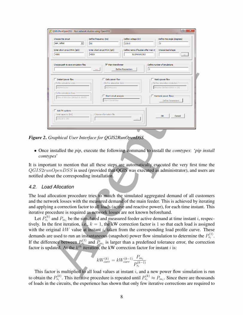
Acce
pted
fit the feederrsquos actual demand as presented in Section 52 A similar procedure is carried out forthe reactive power curve fitting
It is expected that information from smart meters will improve the load allocation accuracy tothe point that only a small correction will be applied to non-monitored loads and this will alsoreduce the number of iterations This load allocation is the first step before running any othernetwork study defined hereafter
43 Types of Network Studies
This section provides some details of the network studies currently carried out in QGIS poweredby OpenDSS The results of these studies are stored according to the userrsquos needs in csv files
bull Snapshot Power Flows This is the simplest study to analyze the network conditions duringa specific instant (eg peak demand and minimum load) This approach however mightresult in under or overestimation of network conditions particularly when considering thevariability of renewable energy sources (eg photovoltaic systems) and loads (eg electricvehicles) In order to run a power flow the user must select the corresponding snapshot box(see Fig 2) and define the date (ddmmyyyy) and time (hhmm) of the simulationIf the user sets a time that is different to the resolution of the simulation the plugin will findthe nearest available simulation instant For instance if the user defines 1805 h in a 15minute resolution the simulation will actually be executed for 1800 h
bull Daily Power Flows This corresponds to time-series daily power flows This type of study isvery helpful to quantify the impacts of variable sources and loads The user needs to definethe date (ddmmyyyy) of the year to be assessed with a given time resolution For a yearlypower flow the user simply defines the year of interest
bull Short circuits In this study the user must define the bus name and phases to be short circuitedThe user can also define a list of bus names and the plugin will create a fault for each bus inOpenDSS
bull Harmonic Power Flows This study is crucial to assess the quality of the service as well as tounderstand the impact of harmonic distortion produced by loads and sources on distributionnetworks This also allows determining the propagation of current components of frequencyother than the fundamental and the resultant distortion of the voltage waveform If this studyis selected the user must define the number of harmonics to be assessed and the spectrum ofeach load and source
These studies can be used to assess the impact of high rooftop PV penetration in the distributionnetwork For this the user must enable this option at the bottom of the GUI as shown in Fig 2Here it is required to define the total capacity to be installed in the circuit and upload a csvfile with the PV capacity for each customer type and monthly energy consumption level Thelist of PV capacities may be the result of a socio-economic study or based on historical data Inthe first case the user knows the most beneficial PV capacity for each customer In the secondcase the user may know the most common PV capacity installed by residential commercial andindustrial customers This csv file is then used to distribute the circuitrsquos total PV capacity amongsome randomly selected customers The plugin will search for the customerrsquos monthly energyconsumption and allocate the corresponding PV capacity This allocation stops when the circuitrsquostotal capacity is met
9
Acce
pted
SubstationMV lineMVLV TxLV line
(a) Original DN model in GIS
(b) Resulting DN model in OpenDSS
Figure 3 Translation of QGIS model to OpenDSS
5 Demonstration
51 Circuit Builder
This section presents a demonstration of the QGIS2OpenDSS tool It presents the translation ofa real 345 kV distribution circuit available in the GIS model of CNFL one of the largest powerutilities in Costa Rica This model includes 2168 MV line sections 7028 LV (secondary) linesections 512 MVLV transformers and 13323 LV loads all of them stored in different layersAccording to the GIS there are 84 km of MV line sections and 215 km of LV line sectionsFig 3(a) presents the GIS model of the circuit section provided by CNFL The GIS files includeall attributes required to run the plugin as explained in Section 31
After selecting the appropriate layers in the GUI the plugin creates the OpenDSS files in lessthan 2 minutes on a PC Intel Rcopy Core i5 4GB RAM 32 bits
10
Acce
ptedLV line
MV line
Transformer
Figure 4 Visualization of bus names in GIS
The first run of QGIS2OpenDSS resulted in a model with errors that would result in manyproblems if used in OpenDSS The plugin reported 12 disconnected MV line sections 18 erroneousphase designations of MV lines two three-phase transformers connected to single-phase MV lines12 disconnected LV line sections and 32 disconnected LV loads Additionally the plugin reported2 transformers with a 0 kVA capacity After these errors were corrected in the GIS database asecond run reported no more errors in the QGIS log message Fig 3(b) presents the resultingcircuit plot in OpenDSS It is seen that the engineering model truly represents the GIS modelThe small differences are explained by the fact that the resulting OpenDSS model does not usepolylines as the GIS model does
The plugin output includes the masterdss file accompanied by the dss files of lines transform-ers and loads definitions In addition the tool creates a csv file containing the list of the networkbuses and their coordinates This file can be used to create a GIS layer to visualize the resultingbus names in QGIS For illustration purposes Fig 4 presents the visualization of some MV andLV bus names defined by the plugin Note that MV and LV bus names have different bus countersHaving the bus names in the GIS is very helpful when analyzing the OpenDSS simulation resultsas will be explained in Section 53
Table 1 presents the time requirements of the plugin to connect the DN elements according tothe spatial coordinates The remaining time is consumed by data reading data processing and errordetections Note that most of the runtime is consumed by the connectivity of the LV line sectionsand service cables The more line sections the longer it takes to kdtree to identify connectivity ofDN elements
11
Acce
pted
Table 1 Connectivity of DN elements
Process Time [s]MV line sections 281
MV lines with transformers 102Transformers with LV line sections 261
LV line sections 901LV lines with service cables 1120
LV lines with loads 368Service cables 2079
Service cables with loads 762
52 Load profile allocation and correction
Based on the monthly energy consumption of customers the QGIS2OpenDSS allocated a typicaldemand profile to each load Almost all loads consume 300 kWh or less Information about cus-tomer types were not available for this circuit however and given that such small energy consump-tions are typical for residential customers only it is considered in this illustration that all customersare residential In total the plugin allocated 135 load profiles among the 13323 customers
As explained in Section 42 these curves are corrected by an iterative process to match the sim-ulated circuit demand with the actual load curve provided by the user Here QGIS2runOpenDSSapplies the same correction factor to all loads In this way the sum of all loads plus the circuitlosses equals the measured demand of the feeder at each time instant
Figure 5 presents the adjustment of one of the 135 load profiles Note that the adjusted curvemaintains the pattern of the original profile and only few corrections are required during the loadallocation process Here the original load profile is scaled up or down at different time instantsdepending on the circuitrsquos actual demand As stated before the correction is small because a) theoriginal load profile truly characterizes the typical behavior of the corresponding load and b) anycorrection is distributed among the 13323 customers in the circuit Certainly the use of smartmeters will further improve the accuracy of simulations as customers will be assigned with theiractual load profiles and the allocation will be limited to those customers without smart meters
The result of the load profile correction is presented in Fig 6 for an arbitrarily selected dayNote that the simulation equals the measured load profile In this demonstration all loads wereassigned with a constant impedance model but any other load model could have been includedinstead
53 Illustrative Network Studies
This section illustrates some analysis that can be carried out using QGIS2RunOpenDSS The pur-pose of this section is to demonstrate different types of detailed studies that can be achieved by theintegration of OpenDSS and QGIS The results are not analyzed in detail as this is out of the scopeof the paper Due to space limitations only three studies are presented snapshot daily and PVimpact
The first illustrative analysis carried out is the snapshot power flow In this case it is required tocheck the LV bus voltages at 1900 h (peak load condition) For this the instant power flow optionwas used along with day and hour of interest as shown in Fig 2 The plugin alerts the user whenthe simulation is over This simulation takes about 2 s due to the massive number of LV buses
12
Acce
pted
0000 0300 0600 0900 1200 1500 1800 2100 0000
0
05
1
15
2
25
3
35
Time
Dem
and
kWoriginaladjusted
Figure 5 Correction of individual load profile carried out by QGIS2runOpenDSS
0000 0300 0600 0900 1200 1500 1800 2100 0000
6
8
10
12
14
16
18
Time
Dem
and
MW
MeasuredSimulated
Figure 6 Comparison of actual versus simulated feederrsquos load profile
13
Acce
pted094 095 096 097 098 099 1 101 102 103 104 105 106
0
500
1000
1500
2000
2500
3000
Voltage pu
Num
bero
fbus
es
Figure 7 LV bus voltages at peak load (snapshot power flow)
This includes the time needed to correct the original load profilesFigure 7 shows the histogram of LV bus voltages as a result of the snapshot power flow simula-
tion Note that none of the buses are beyond theplusmn5 bandwidth In fact most LV buses are withinplusmn3 of nominal voltage QGIS2RunOpenDSS can also display the current and voltages throughmonitored transformers and lines However due to space limitations they have not been included
To run a daily power flow the user must select this option in the GUI of QGIS2RunOpenDSSThe daily simulation (in a 15-min resolution) takes on average 50 s including the runtime of theload allocation algorithm QGIS2RunOpenDSS allows users to export the simulation results of anyelement (transformer line andor cable) in the circuit For this the user only needs to select thecorresponding monitor from the pull-down list of monitors Fig 8 presents the variation of allLV buses throughout the day All results are presented in box plots which include median value(horizontal line) first and third quartile and the outliers As can be seen all bus voltages remainwithin the acceptable band of operation even at peak load conditions The buses with the highestvoltages are those close to the MVLV transformers while the lower voltages are found at the tailsof the secondary circuits The lower voltages occur at peak loading conditions Note also that thebus voltages presented in Fig 7 are in agreement with the box plot at 1900 h
54 PV allocation and impact study
Table 2 presents the PV capacities chosen for residential customers based on their monthly energyconsumption This information was included in a csv file to be read by QGIS2runOpenDSSas presented in Fig 2 According to a socio-economic study carried out for the power utilityresidential customers with a monthly energy consumption equal or less than 300 kWh will notinstall a PV system Based on this the maximum expected installed capacity of rooftop PV systems
14
Acce
pted0000 0300 0600 0900 1200 1500 1800 2100 0000
095
1
105
Volta
gep
u
Time
Figure 8 LV bus voltages through out the day (daily power flow)
Table 2 Information required by plugin to assign the PV systems
Monthly consumption (kWh) Capacity (kW)gt 300 000
300 - 320 075330 - 360 100370 - 380 125390 - 680 325690 - 950 525
is 1700 kW throughout the circuitThe plugin randomly allocates these PV systems among the customers until the requested pen-
etration level is met Figure 9 presents the simulation result of the active power demand when the1700 kW are installed in the circuit When compared to the base case it is seen that the circuitdemanded less power from 600 to 1800 h This small penetration level is not expected to largelyaffect the operation of the network
Although not shown here the voltages increased during the day thanks to the active powerinjection of rooftop PV systems when compared to the base case
6 Discussion
As demonstrated before detailed studies of future DNs with LCTs will be easily carried out thanksto the integration of GIS and advanced simulation tools such as OpenDSS In addition results ofsocio-economic studies can help to simulate more realistic scenarios These tools could also beextended to assess the network condition in the presence of PV and energy storage systems alongwith irradiation layers to better represent the solar potential at a given geographic area In addition
15
Acce
pted0000 0300 0600 0900 1200 1500 1800 2100 0000
6
8
10
12
14
16
18
Time
Dem
and
MW
0 kW1700 kW
Figure 9 Feederrsquos load profile with PVs
the integration of transportation layers could also be used when studying the integration of ElectricVehicles (EVs) into the grid and the optimal location of fast charging stations
The key to carry out these studies is high quality GIS data This information needs to becleaned from spurious data that could result in unrealistic engineering network models Indeedthe correction of errors is not straightforward and requires knowledge of how GIS network modelsare built and how they have to be translated for power engineering uses
From authors experience most errors are found in secondary systems due to the presence ofmany short line segments and also because LV systems were not included in traditional studies runby power utilities To overcome this the aforementioned tools should be complemented with newplugins able to automatically correct frequently found errors such as disconnected LV elements ornonexistent connections among different secondary circuits For example Kd-tree could be used toautomatically identify service cables inside a circle centered at the disconnected load If a servicecable was found inside the circle the coordinate of the disconnected load should be corrected tomatch the coordinate of the service cable end Similar procedure could be carried out to connectline segments Unfortunately not all disconnection problems will be automatically corrected assome cases require human intervention to decide where to connect a disconnected element
The identification of connected elements is likely to be the most important step when buildingthe engineering model in OpenDSS As reported in Section 32 this task was successfully achievedthanks to the Kd-tree algorithm However the authors believe that the same task could be accom-plished by more efficient computational tools based on Graph theory In this regard future workwill focus on reducing the time requirements for the connectivity of network elements
To take full advantages of GIS software capabilities future work will also be focused on vi-sualization of simulation results This is the simulation results currently shown in plots will be
16
Acce
pted
visualized in the GIS network model For instance overvoltages due to massive integration ofPVs or under voltages caused by high EV penetrations at LV level could be represented in theGIS environment by heatmaps or different scale colors In addition some GIS properties of DNelements could be also modified (eg line thickness or point size) to represent highly loaded oreven overloaded lines and transformers
Finally detailed simulations of smart distribution networks will be further improved when loadprofiles from smart meters replace the typical profiles currently used by the developed tools Thiswill also require the integration of databases fed from smart meters with the QGIS software
7 Conclusion
This paper has presented the integration of OpenDSS with an open source GIS platform to carryout easier and more efficient studies of distribution networks Two software plugins were created toextract GIS data to automatically build a distribution network engineering model and run OpenDSSas an embedded tool in the GIS platform These plugins aim at facilitating the studies that powerengineers have to run in the short term by integrating free and open source GIS software withexisting free and open source power engineering software In addition they have great potential tobe used for educational purposes at university level and for training of junior engineers
The performance of the simulation tool has been demonstrated on a real circuit in Costa Ricawith more than 10000 customers The illustrative examples highlight the efficiency and conve-nience of the tool to perform detailed network studies
The release of these tools is expected to bring new opportunities to power utilities researchlaboratories and universities to test and simulate novel smart grid solutions with more realisticnetwork models In addition future collaborations from other users will enhance the robustnessand generality of the tools
8 Acknowledgment
The authors would like to thank CNFL for providing the GIS database of the analyzed circuit
9 References
[1] R Arritt and R Dugan ldquoDistribution System Analysis and the Future Smart Gridrdquo IEEETransactions on Industry Applications vol 47 no 6 pp 2343ndash2350 Nov 2011
[2] G Shirek B A Lassiter W Carr and W H Kersting ldquoModeling Secondary Services inEngineering and Mappingrdquo IEEE Transactions on Industry Applications vol 48 no 1 pp254ndash262 Feb 2012
[3] A Navarro-Espinosa L Ochoa R Shaw and D Randles ldquoReconstruction of Low Volt-age Distribution Networks From GIS Data to Power Flow Modelsrdquo in 23rd InternationalConference on Electricity Distribution no 1273 CIRED 2015
[4] B Meehan GIS for Enhanced Electric Utility Performance Artech House 2013
[5] R Brenes A Arguello J Quiros-Tortos and G Valverde ldquoDistribution Network ElementModel Parameters Creation of Databaserdquo in IEEE CONCAPAN Nov 2016
17
Acce
pted
[6] A Crossland N Wade and D Jones ldquoExtraction of 9163 Real LV Network Models fromDNO GIS Database to Assess Overvoltage from PV and Consequent Mitigation Measuresrdquoin 23rd International Conference on Electricity Distribution no 0915 CIRED 2015
[7] S Lazarou V Vita P Karampelas and L Ekonomou ldquoA Power System Simulation Platformfor Planning and Evaluating Distributed Generation Systems based on GISrdquo Energy Systemsvol 4 no 4 pp 379ndash391 Apr 2013
[8] F Milano Power System Modelling and Scripting Springer 2010
[9] R Dugan and T E McDermott ldquoAn Open Source Platform for Collaborating on Smart GridResearchrdquo in IEEE PES General Meeting 2011
[10] D P Chassin K Schneider and C Gerkensmeyer ldquoGridLAB-D An Open-Source PowerSystems Modeling and Simulation Environmentrdquo in 2008 IEEEPES Transmission and Dis-tribution Conference and Exposition April 2008 pp 1ndash5
[11] EPERLab ldquoRelease of plugins Integration of Open Source Tools for StudyingLarge-Scale Distribution Networksrdquo 2017 [Online] Available httpeperlabeieucraccrdocuments [Available from Jul 2017]
[12] Task Force on Open Source Software for Power Systems Open Source Software IEEEPSACE Committee [Online] Available httpewhieeeorgcmtepsaceCAMS taskforcesoftwarehtm
[13] P Bolstad GIS Fundementals a First Text on Geographical Information Systems 4th edMinnesota EEUU Eider Press 2002
[14] QGIS PyQGIS Developer Cookbook February 2016 [Online] Available httpdocsqgisorg
[15] R Dugan Reference Guide The Open Distribution System Simulator EPRI June 2013
[16] W H Kersting Distribution System Modeling and Analysis 3rd ed CRC Press 2012
[17] T Short Electric Power Distribution Handbook CRC 2004
[18] J L Bentley ldquoMultidimensional Binary Search Trees Used for Associative Searchingrdquo Com-munications of the ACM vol 18 no 9 pp 509ndash517 Sept 1975
[19] J Quiros-Tortos A Arguello and G Valverde ldquoStatistical Analysis of Residential DemandBehavior in Costa Rica Creation of Load Profilesrdquo in IEEE CONCAPAN Nov 2016
18
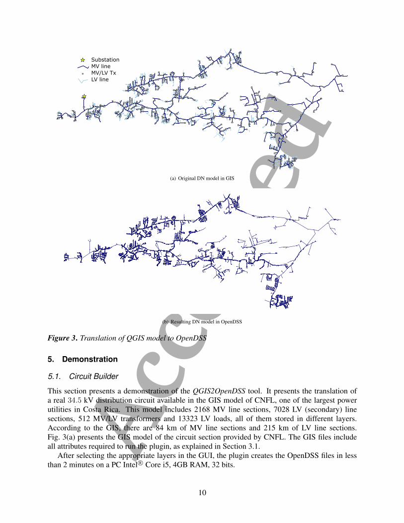
Acce
pted
SubstationMV lineMVLV TxLV line
(a) Original DN model in GIS
(b) Resulting DN model in OpenDSS
Figure 3 Translation of QGIS model to OpenDSS
5 Demonstration
51 Circuit Builder
This section presents a demonstration of the QGIS2OpenDSS tool It presents the translation ofa real 345 kV distribution circuit available in the GIS model of CNFL one of the largest powerutilities in Costa Rica This model includes 2168 MV line sections 7028 LV (secondary) linesections 512 MVLV transformers and 13323 LV loads all of them stored in different layersAccording to the GIS there are 84 km of MV line sections and 215 km of LV line sectionsFig 3(a) presents the GIS model of the circuit section provided by CNFL The GIS files includeall attributes required to run the plugin as explained in Section 31
After selecting the appropriate layers in the GUI the plugin creates the OpenDSS files in lessthan 2 minutes on a PC Intel Rcopy Core i5 4GB RAM 32 bits
10
Acce
ptedLV line
MV line
Transformer
Figure 4 Visualization of bus names in GIS
The first run of QGIS2OpenDSS resulted in a model with errors that would result in manyproblems if used in OpenDSS The plugin reported 12 disconnected MV line sections 18 erroneousphase designations of MV lines two three-phase transformers connected to single-phase MV lines12 disconnected LV line sections and 32 disconnected LV loads Additionally the plugin reported2 transformers with a 0 kVA capacity After these errors were corrected in the GIS database asecond run reported no more errors in the QGIS log message Fig 3(b) presents the resultingcircuit plot in OpenDSS It is seen that the engineering model truly represents the GIS modelThe small differences are explained by the fact that the resulting OpenDSS model does not usepolylines as the GIS model does
The plugin output includes the masterdss file accompanied by the dss files of lines transform-ers and loads definitions In addition the tool creates a csv file containing the list of the networkbuses and their coordinates This file can be used to create a GIS layer to visualize the resultingbus names in QGIS For illustration purposes Fig 4 presents the visualization of some MV andLV bus names defined by the plugin Note that MV and LV bus names have different bus countersHaving the bus names in the GIS is very helpful when analyzing the OpenDSS simulation resultsas will be explained in Section 53
Table 1 presents the time requirements of the plugin to connect the DN elements according tothe spatial coordinates The remaining time is consumed by data reading data processing and errordetections Note that most of the runtime is consumed by the connectivity of the LV line sectionsand service cables The more line sections the longer it takes to kdtree to identify connectivity ofDN elements
11
Acce
pted
Table 1 Connectivity of DN elements
Process Time [s]MV line sections 281
MV lines with transformers 102Transformers with LV line sections 261
LV line sections 901LV lines with service cables 1120
LV lines with loads 368Service cables 2079
Service cables with loads 762
52 Load profile allocation and correction
Based on the monthly energy consumption of customers the QGIS2OpenDSS allocated a typicaldemand profile to each load Almost all loads consume 300 kWh or less Information about cus-tomer types were not available for this circuit however and given that such small energy consump-tions are typical for residential customers only it is considered in this illustration that all customersare residential In total the plugin allocated 135 load profiles among the 13323 customers
As explained in Section 42 these curves are corrected by an iterative process to match the sim-ulated circuit demand with the actual load curve provided by the user Here QGIS2runOpenDSSapplies the same correction factor to all loads In this way the sum of all loads plus the circuitlosses equals the measured demand of the feeder at each time instant
Figure 5 presents the adjustment of one of the 135 load profiles Note that the adjusted curvemaintains the pattern of the original profile and only few corrections are required during the loadallocation process Here the original load profile is scaled up or down at different time instantsdepending on the circuitrsquos actual demand As stated before the correction is small because a) theoriginal load profile truly characterizes the typical behavior of the corresponding load and b) anycorrection is distributed among the 13323 customers in the circuit Certainly the use of smartmeters will further improve the accuracy of simulations as customers will be assigned with theiractual load profiles and the allocation will be limited to those customers without smart meters
The result of the load profile correction is presented in Fig 6 for an arbitrarily selected dayNote that the simulation equals the measured load profile In this demonstration all loads wereassigned with a constant impedance model but any other load model could have been includedinstead
53 Illustrative Network Studies
This section illustrates some analysis that can be carried out using QGIS2RunOpenDSS The pur-pose of this section is to demonstrate different types of detailed studies that can be achieved by theintegration of OpenDSS and QGIS The results are not analyzed in detail as this is out of the scopeof the paper Due to space limitations only three studies are presented snapshot daily and PVimpact
The first illustrative analysis carried out is the snapshot power flow In this case it is required tocheck the LV bus voltages at 1900 h (peak load condition) For this the instant power flow optionwas used along with day and hour of interest as shown in Fig 2 The plugin alerts the user whenthe simulation is over This simulation takes about 2 s due to the massive number of LV buses
12
Acce
pted
0000 0300 0600 0900 1200 1500 1800 2100 0000
0
05
1
15
2
25
3
35
Time
Dem
and
kWoriginaladjusted
Figure 5 Correction of individual load profile carried out by QGIS2runOpenDSS
0000 0300 0600 0900 1200 1500 1800 2100 0000
6
8
10
12
14
16
18
Time
Dem
and
MW
MeasuredSimulated
Figure 6 Comparison of actual versus simulated feederrsquos load profile
13
Acce
pted094 095 096 097 098 099 1 101 102 103 104 105 106
0
500
1000
1500
2000
2500
3000
Voltage pu
Num
bero
fbus
es
Figure 7 LV bus voltages at peak load (snapshot power flow)
This includes the time needed to correct the original load profilesFigure 7 shows the histogram of LV bus voltages as a result of the snapshot power flow simula-
tion Note that none of the buses are beyond theplusmn5 bandwidth In fact most LV buses are withinplusmn3 of nominal voltage QGIS2RunOpenDSS can also display the current and voltages throughmonitored transformers and lines However due to space limitations they have not been included
To run a daily power flow the user must select this option in the GUI of QGIS2RunOpenDSSThe daily simulation (in a 15-min resolution) takes on average 50 s including the runtime of theload allocation algorithm QGIS2RunOpenDSS allows users to export the simulation results of anyelement (transformer line andor cable) in the circuit For this the user only needs to select thecorresponding monitor from the pull-down list of monitors Fig 8 presents the variation of allLV buses throughout the day All results are presented in box plots which include median value(horizontal line) first and third quartile and the outliers As can be seen all bus voltages remainwithin the acceptable band of operation even at peak load conditions The buses with the highestvoltages are those close to the MVLV transformers while the lower voltages are found at the tailsof the secondary circuits The lower voltages occur at peak loading conditions Note also that thebus voltages presented in Fig 7 are in agreement with the box plot at 1900 h
54 PV allocation and impact study
Table 2 presents the PV capacities chosen for residential customers based on their monthly energyconsumption This information was included in a csv file to be read by QGIS2runOpenDSSas presented in Fig 2 According to a socio-economic study carried out for the power utilityresidential customers with a monthly energy consumption equal or less than 300 kWh will notinstall a PV system Based on this the maximum expected installed capacity of rooftop PV systems
14
Acce
pted0000 0300 0600 0900 1200 1500 1800 2100 0000
095
1
105
Volta
gep
u
Time
Figure 8 LV bus voltages through out the day (daily power flow)
Table 2 Information required by plugin to assign the PV systems
Monthly consumption (kWh) Capacity (kW)gt 300 000
300 - 320 075330 - 360 100370 - 380 125390 - 680 325690 - 950 525
is 1700 kW throughout the circuitThe plugin randomly allocates these PV systems among the customers until the requested pen-
etration level is met Figure 9 presents the simulation result of the active power demand when the1700 kW are installed in the circuit When compared to the base case it is seen that the circuitdemanded less power from 600 to 1800 h This small penetration level is not expected to largelyaffect the operation of the network
Although not shown here the voltages increased during the day thanks to the active powerinjection of rooftop PV systems when compared to the base case
6 Discussion
As demonstrated before detailed studies of future DNs with LCTs will be easily carried out thanksto the integration of GIS and advanced simulation tools such as OpenDSS In addition results ofsocio-economic studies can help to simulate more realistic scenarios These tools could also beextended to assess the network condition in the presence of PV and energy storage systems alongwith irradiation layers to better represent the solar potential at a given geographic area In addition
15
Acce
pted0000 0300 0600 0900 1200 1500 1800 2100 0000
6
8
10
12
14
16
18
Time
Dem
and
MW
0 kW1700 kW
Figure 9 Feederrsquos load profile with PVs
the integration of transportation layers could also be used when studying the integration of ElectricVehicles (EVs) into the grid and the optimal location of fast charging stations
The key to carry out these studies is high quality GIS data This information needs to becleaned from spurious data that could result in unrealistic engineering network models Indeedthe correction of errors is not straightforward and requires knowledge of how GIS network modelsare built and how they have to be translated for power engineering uses
From authors experience most errors are found in secondary systems due to the presence ofmany short line segments and also because LV systems were not included in traditional studies runby power utilities To overcome this the aforementioned tools should be complemented with newplugins able to automatically correct frequently found errors such as disconnected LV elements ornonexistent connections among different secondary circuits For example Kd-tree could be used toautomatically identify service cables inside a circle centered at the disconnected load If a servicecable was found inside the circle the coordinate of the disconnected load should be corrected tomatch the coordinate of the service cable end Similar procedure could be carried out to connectline segments Unfortunately not all disconnection problems will be automatically corrected assome cases require human intervention to decide where to connect a disconnected element
The identification of connected elements is likely to be the most important step when buildingthe engineering model in OpenDSS As reported in Section 32 this task was successfully achievedthanks to the Kd-tree algorithm However the authors believe that the same task could be accom-plished by more efficient computational tools based on Graph theory In this regard future workwill focus on reducing the time requirements for the connectivity of network elements
To take full advantages of GIS software capabilities future work will also be focused on vi-sualization of simulation results This is the simulation results currently shown in plots will be
16
Acce
pted
visualized in the GIS network model For instance overvoltages due to massive integration ofPVs or under voltages caused by high EV penetrations at LV level could be represented in theGIS environment by heatmaps or different scale colors In addition some GIS properties of DNelements could be also modified (eg line thickness or point size) to represent highly loaded oreven overloaded lines and transformers
Finally detailed simulations of smart distribution networks will be further improved when loadprofiles from smart meters replace the typical profiles currently used by the developed tools Thiswill also require the integration of databases fed from smart meters with the QGIS software
7 Conclusion
This paper has presented the integration of OpenDSS with an open source GIS platform to carryout easier and more efficient studies of distribution networks Two software plugins were created toextract GIS data to automatically build a distribution network engineering model and run OpenDSSas an embedded tool in the GIS platform These plugins aim at facilitating the studies that powerengineers have to run in the short term by integrating free and open source GIS software withexisting free and open source power engineering software In addition they have great potential tobe used for educational purposes at university level and for training of junior engineers
The performance of the simulation tool has been demonstrated on a real circuit in Costa Ricawith more than 10000 customers The illustrative examples highlight the efficiency and conve-nience of the tool to perform detailed network studies
The release of these tools is expected to bring new opportunities to power utilities researchlaboratories and universities to test and simulate novel smart grid solutions with more realisticnetwork models In addition future collaborations from other users will enhance the robustnessand generality of the tools
8 Acknowledgment
The authors would like to thank CNFL for providing the GIS database of the analyzed circuit
9 References
[1] R Arritt and R Dugan ldquoDistribution System Analysis and the Future Smart Gridrdquo IEEETransactions on Industry Applications vol 47 no 6 pp 2343ndash2350 Nov 2011
[2] G Shirek B A Lassiter W Carr and W H Kersting ldquoModeling Secondary Services inEngineering and Mappingrdquo IEEE Transactions on Industry Applications vol 48 no 1 pp254ndash262 Feb 2012
[3] A Navarro-Espinosa L Ochoa R Shaw and D Randles ldquoReconstruction of Low Volt-age Distribution Networks From GIS Data to Power Flow Modelsrdquo in 23rd InternationalConference on Electricity Distribution no 1273 CIRED 2015
[4] B Meehan GIS for Enhanced Electric Utility Performance Artech House 2013
[5] R Brenes A Arguello J Quiros-Tortos and G Valverde ldquoDistribution Network ElementModel Parameters Creation of Databaserdquo in IEEE CONCAPAN Nov 2016
17
Acce
pted
[6] A Crossland N Wade and D Jones ldquoExtraction of 9163 Real LV Network Models fromDNO GIS Database to Assess Overvoltage from PV and Consequent Mitigation Measuresrdquoin 23rd International Conference on Electricity Distribution no 0915 CIRED 2015
[7] S Lazarou V Vita P Karampelas and L Ekonomou ldquoA Power System Simulation Platformfor Planning and Evaluating Distributed Generation Systems based on GISrdquo Energy Systemsvol 4 no 4 pp 379ndash391 Apr 2013
[8] F Milano Power System Modelling and Scripting Springer 2010
[9] R Dugan and T E McDermott ldquoAn Open Source Platform for Collaborating on Smart GridResearchrdquo in IEEE PES General Meeting 2011
[10] D P Chassin K Schneider and C Gerkensmeyer ldquoGridLAB-D An Open-Source PowerSystems Modeling and Simulation Environmentrdquo in 2008 IEEEPES Transmission and Dis-tribution Conference and Exposition April 2008 pp 1ndash5
[11] EPERLab ldquoRelease of plugins Integration of Open Source Tools for StudyingLarge-Scale Distribution Networksrdquo 2017 [Online] Available httpeperlabeieucraccrdocuments [Available from Jul 2017]
[12] Task Force on Open Source Software for Power Systems Open Source Software IEEEPSACE Committee [Online] Available httpewhieeeorgcmtepsaceCAMS taskforcesoftwarehtm
[13] P Bolstad GIS Fundementals a First Text on Geographical Information Systems 4th edMinnesota EEUU Eider Press 2002
[14] QGIS PyQGIS Developer Cookbook February 2016 [Online] Available httpdocsqgisorg
[15] R Dugan Reference Guide The Open Distribution System Simulator EPRI June 2013
[16] W H Kersting Distribution System Modeling and Analysis 3rd ed CRC Press 2012
[17] T Short Electric Power Distribution Handbook CRC 2004
[18] J L Bentley ldquoMultidimensional Binary Search Trees Used for Associative Searchingrdquo Com-munications of the ACM vol 18 no 9 pp 509ndash517 Sept 1975
[19] J Quiros-Tortos A Arguello and G Valverde ldquoStatistical Analysis of Residential DemandBehavior in Costa Rica Creation of Load Profilesrdquo in IEEE CONCAPAN Nov 2016
18
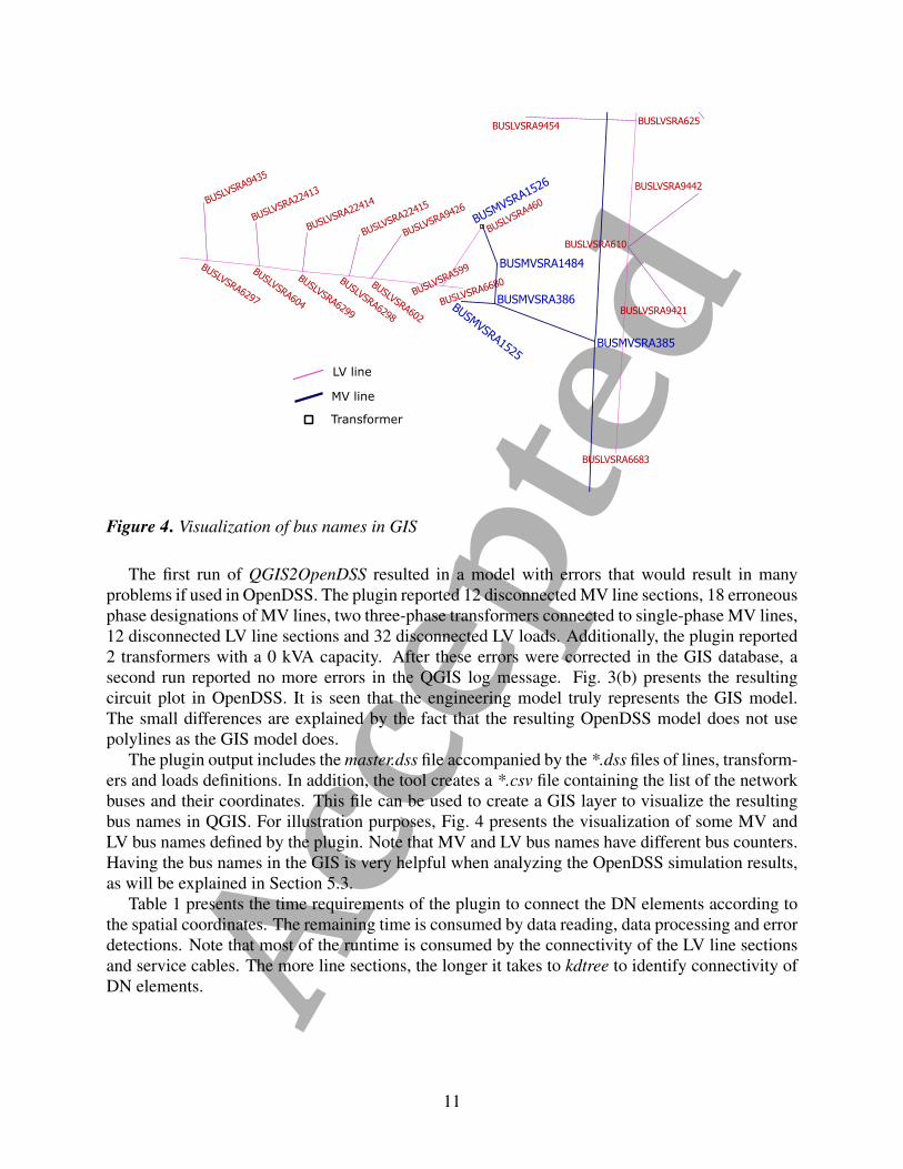
Acce
pted
Table 1 Connectivity of DN elements
Process Time [s]MV line sections 281
MV lines with transformers 102Transformers with LV line sections 261
LV line sections 901LV lines with service cables 1120
LV lines with loads 368Service cables 2079
Service cables with loads 762
52 Load profile allocation and correction
Based on the monthly energy consumption of customers the QGIS2OpenDSS allocated a typicaldemand profile to each load Almost all loads consume 300 kWh or less Information about cus-tomer types were not available for this circuit however and given that such small energy consump-tions are typical for residential customers only it is considered in this illustration that all customersare residential In total the plugin allocated 135 load profiles among the 13323 customers
As explained in Section 42 these curves are corrected by an iterative process to match the sim-ulated circuit demand with the actual load curve provided by the user Here QGIS2runOpenDSSapplies the same correction factor to all loads In this way the sum of all loads plus the circuitlosses equals the measured demand of the feeder at each time instant
Figure 5 presents the adjustment of one of the 135 load profiles Note that the adjusted curvemaintains the pattern of the original profile and only few corrections are required during the loadallocation process Here the original load profile is scaled up or down at different time instantsdepending on the circuitrsquos actual demand As stated before the correction is small because a) theoriginal load profile truly characterizes the typical behavior of the corresponding load and b) anycorrection is distributed among the 13323 customers in the circuit Certainly the use of smartmeters will further improve the accuracy of simulations as customers will be assigned with theiractual load profiles and the allocation will be limited to those customers without smart meters
The result of the load profile correction is presented in Fig 6 for an arbitrarily selected dayNote that the simulation equals the measured load profile In this demonstration all loads wereassigned with a constant impedance model but any other load model could have been includedinstead
53 Illustrative Network Studies
This section illustrates some analysis that can be carried out using QGIS2RunOpenDSS The pur-pose of this section is to demonstrate different types of detailed studies that can be achieved by theintegration of OpenDSS and QGIS The results are not analyzed in detail as this is out of the scopeof the paper Due to space limitations only three studies are presented snapshot daily and PVimpact
The first illustrative analysis carried out is the snapshot power flow In this case it is required tocheck the LV bus voltages at 1900 h (peak load condition) For this the instant power flow optionwas used along with day and hour of interest as shown in Fig 2 The plugin alerts the user whenthe simulation is over This simulation takes about 2 s due to the massive number of LV buses
12
Acce
pted
0000 0300 0600 0900 1200 1500 1800 2100 0000
0
05
1
15
2
25
3
35
Time
Dem
and
kWoriginaladjusted
Figure 5 Correction of individual load profile carried out by QGIS2runOpenDSS
0000 0300 0600 0900 1200 1500 1800 2100 0000
6
8
10
12
14
16
18
Time
Dem
and
MW
MeasuredSimulated
Figure 6 Comparison of actual versus simulated feederrsquos load profile
13
Acce
pted094 095 096 097 098 099 1 101 102 103 104 105 106
0
500
1000
1500
2000
2500
3000
Voltage pu
Num
bero
fbus
es
Figure 7 LV bus voltages at peak load (snapshot power flow)
This includes the time needed to correct the original load profilesFigure 7 shows the histogram of LV bus voltages as a result of the snapshot power flow simula-
tion Note that none of the buses are beyond theplusmn5 bandwidth In fact most LV buses are withinplusmn3 of nominal voltage QGIS2RunOpenDSS can also display the current and voltages throughmonitored transformers and lines However due to space limitations they have not been included
To run a daily power flow the user must select this option in the GUI of QGIS2RunOpenDSSThe daily simulation (in a 15-min resolution) takes on average 50 s including the runtime of theload allocation algorithm QGIS2RunOpenDSS allows users to export the simulation results of anyelement (transformer line andor cable) in the circuit For this the user only needs to select thecorresponding monitor from the pull-down list of monitors Fig 8 presents the variation of allLV buses throughout the day All results are presented in box plots which include median value(horizontal line) first and third quartile and the outliers As can be seen all bus voltages remainwithin the acceptable band of operation even at peak load conditions The buses with the highestvoltages are those close to the MVLV transformers while the lower voltages are found at the tailsof the secondary circuits The lower voltages occur at peak loading conditions Note also that thebus voltages presented in Fig 7 are in agreement with the box plot at 1900 h
54 PV allocation and impact study
Table 2 presents the PV capacities chosen for residential customers based on their monthly energyconsumption This information was included in a csv file to be read by QGIS2runOpenDSSas presented in Fig 2 According to a socio-economic study carried out for the power utilityresidential customers with a monthly energy consumption equal or less than 300 kWh will notinstall a PV system Based on this the maximum expected installed capacity of rooftop PV systems
14
Acce
pted0000 0300 0600 0900 1200 1500 1800 2100 0000
095
1
105
Volta
gep
u
Time
Figure 8 LV bus voltages through out the day (daily power flow)
Table 2 Information required by plugin to assign the PV systems
Monthly consumption (kWh) Capacity (kW)gt 300 000
300 - 320 075330 - 360 100370 - 380 125390 - 680 325690 - 950 525
is 1700 kW throughout the circuitThe plugin randomly allocates these PV systems among the customers until the requested pen-
etration level is met Figure 9 presents the simulation result of the active power demand when the1700 kW are installed in the circuit When compared to the base case it is seen that the circuitdemanded less power from 600 to 1800 h This small penetration level is not expected to largelyaffect the operation of the network
Although not shown here the voltages increased during the day thanks to the active powerinjection of rooftop PV systems when compared to the base case
6 Discussion
As demonstrated before detailed studies of future DNs with LCTs will be easily carried out thanksto the integration of GIS and advanced simulation tools such as OpenDSS In addition results ofsocio-economic studies can help to simulate more realistic scenarios These tools could also beextended to assess the network condition in the presence of PV and energy storage systems alongwith irradiation layers to better represent the solar potential at a given geographic area In addition
15
Acce
pted0000 0300 0600 0900 1200 1500 1800 2100 0000
6
8
10
12
14
16
18
Time
Dem
and
MW
0 kW1700 kW
Figure 9 Feederrsquos load profile with PVs
the integration of transportation layers could also be used when studying the integration of ElectricVehicles (EVs) into the grid and the optimal location of fast charging stations
The key to carry out these studies is high quality GIS data This information needs to becleaned from spurious data that could result in unrealistic engineering network models Indeedthe correction of errors is not straightforward and requires knowledge of how GIS network modelsare built and how they have to be translated for power engineering uses
From authors experience most errors are found in secondary systems due to the presence ofmany short line segments and also because LV systems were not included in traditional studies runby power utilities To overcome this the aforementioned tools should be complemented with newplugins able to automatically correct frequently found errors such as disconnected LV elements ornonexistent connections among different secondary circuits For example Kd-tree could be used toautomatically identify service cables inside a circle centered at the disconnected load If a servicecable was found inside the circle the coordinate of the disconnected load should be corrected tomatch the coordinate of the service cable end Similar procedure could be carried out to connectline segments Unfortunately not all disconnection problems will be automatically corrected assome cases require human intervention to decide where to connect a disconnected element
The identification of connected elements is likely to be the most important step when buildingthe engineering model in OpenDSS As reported in Section 32 this task was successfully achievedthanks to the Kd-tree algorithm However the authors believe that the same task could be accom-plished by more efficient computational tools based on Graph theory In this regard future workwill focus on reducing the time requirements for the connectivity of network elements
To take full advantages of GIS software capabilities future work will also be focused on vi-sualization of simulation results This is the simulation results currently shown in plots will be
16
Acce
pted
visualized in the GIS network model For instance overvoltages due to massive integration ofPVs or under voltages caused by high EV penetrations at LV level could be represented in theGIS environment by heatmaps or different scale colors In addition some GIS properties of DNelements could be also modified (eg line thickness or point size) to represent highly loaded oreven overloaded lines and transformers
Finally detailed simulations of smart distribution networks will be further improved when loadprofiles from smart meters replace the typical profiles currently used by the developed tools Thiswill also require the integration of databases fed from smart meters with the QGIS software
7 Conclusion
This paper has presented the integration of OpenDSS with an open source GIS platform to carryout easier and more efficient studies of distribution networks Two software plugins were created toextract GIS data to automatically build a distribution network engineering model and run OpenDSSas an embedded tool in the GIS platform These plugins aim at facilitating the studies that powerengineers have to run in the short term by integrating free and open source GIS software withexisting free and open source power engineering software In addition they have great potential tobe used for educational purposes at university level and for training of junior engineers
The performance of the simulation tool has been demonstrated on a real circuit in Costa Ricawith more than 10000 customers The illustrative examples highlight the efficiency and conve-nience of the tool to perform detailed network studies
The release of these tools is expected to bring new opportunities to power utilities researchlaboratories and universities to test and simulate novel smart grid solutions with more realisticnetwork models In addition future collaborations from other users will enhance the robustnessand generality of the tools
8 Acknowledgment
The authors would like to thank CNFL for providing the GIS database of the analyzed circuit
9 References
[1] R Arritt and R Dugan ldquoDistribution System Analysis and the Future Smart Gridrdquo IEEETransactions on Industry Applications vol 47 no 6 pp 2343ndash2350 Nov 2011
[2] G Shirek B A Lassiter W Carr and W H Kersting ldquoModeling Secondary Services inEngineering and Mappingrdquo IEEE Transactions on Industry Applications vol 48 no 1 pp254ndash262 Feb 2012
[3] A Navarro-Espinosa L Ochoa R Shaw and D Randles ldquoReconstruction of Low Volt-age Distribution Networks From GIS Data to Power Flow Modelsrdquo in 23rd InternationalConference on Electricity Distribution no 1273 CIRED 2015
[4] B Meehan GIS for Enhanced Electric Utility Performance Artech House 2013
[5] R Brenes A Arguello J Quiros-Tortos and G Valverde ldquoDistribution Network ElementModel Parameters Creation of Databaserdquo in IEEE CONCAPAN Nov 2016
17
Acce
pted
[6] A Crossland N Wade and D Jones ldquoExtraction of 9163 Real LV Network Models fromDNO GIS Database to Assess Overvoltage from PV and Consequent Mitigation Measuresrdquoin 23rd International Conference on Electricity Distribution no 0915 CIRED 2015
[7] S Lazarou V Vita P Karampelas and L Ekonomou ldquoA Power System Simulation Platformfor Planning and Evaluating Distributed Generation Systems based on GISrdquo Energy Systemsvol 4 no 4 pp 379ndash391 Apr 2013
[8] F Milano Power System Modelling and Scripting Springer 2010
[9] R Dugan and T E McDermott ldquoAn Open Source Platform for Collaborating on Smart GridResearchrdquo in IEEE PES General Meeting 2011
[10] D P Chassin K Schneider and C Gerkensmeyer ldquoGridLAB-D An Open-Source PowerSystems Modeling and Simulation Environmentrdquo in 2008 IEEEPES Transmission and Dis-tribution Conference and Exposition April 2008 pp 1ndash5
[11] EPERLab ldquoRelease of plugins Integration of Open Source Tools for StudyingLarge-Scale Distribution Networksrdquo 2017 [Online] Available httpeperlabeieucraccrdocuments [Available from Jul 2017]
[12] Task Force on Open Source Software for Power Systems Open Source Software IEEEPSACE Committee [Online] Available httpewhieeeorgcmtepsaceCAMS taskforcesoftwarehtm
[13] P Bolstad GIS Fundementals a First Text on Geographical Information Systems 4th edMinnesota EEUU Eider Press 2002
[14] QGIS PyQGIS Developer Cookbook February 2016 [Online] Available httpdocsqgisorg
[15] R Dugan Reference Guide The Open Distribution System Simulator EPRI June 2013
[16] W H Kersting Distribution System Modeling and Analysis 3rd ed CRC Press 2012
[17] T Short Electric Power Distribution Handbook CRC 2004
[18] J L Bentley ldquoMultidimensional Binary Search Trees Used for Associative Searchingrdquo Com-munications of the ACM vol 18 no 9 pp 509ndash517 Sept 1975
[19] J Quiros-Tortos A Arguello and G Valverde ldquoStatistical Analysis of Residential DemandBehavior in Costa Rica Creation of Load Profilesrdquo in IEEE CONCAPAN Nov 2016
18
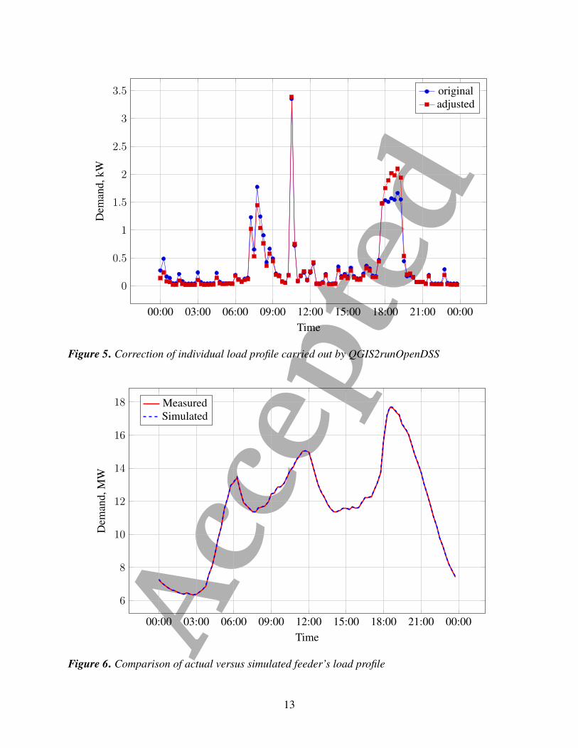
Acce
pted
0000 0300 0600 0900 1200 1500 1800 2100 0000
0
05
1
15
2
25
3
35
Time
Dem
and
kWoriginaladjusted
Figure 5 Correction of individual load profile carried out by QGIS2runOpenDSS
0000 0300 0600 0900 1200 1500 1800 2100 0000
6
8
10
12
14
16
18
Time
Dem
and
MW
MeasuredSimulated
Figure 6 Comparison of actual versus simulated feederrsquos load profile
13
Acce
pted094 095 096 097 098 099 1 101 102 103 104 105 106
0
500
1000
1500
2000
2500
3000
Voltage pu
Num
bero
fbus
es
Figure 7 LV bus voltages at peak load (snapshot power flow)
This includes the time needed to correct the original load profilesFigure 7 shows the histogram of LV bus voltages as a result of the snapshot power flow simula-
tion Note that none of the buses are beyond theplusmn5 bandwidth In fact most LV buses are withinplusmn3 of nominal voltage QGIS2RunOpenDSS can also display the current and voltages throughmonitored transformers and lines However due to space limitations they have not been included
To run a daily power flow the user must select this option in the GUI of QGIS2RunOpenDSSThe daily simulation (in a 15-min resolution) takes on average 50 s including the runtime of theload allocation algorithm QGIS2RunOpenDSS allows users to export the simulation results of anyelement (transformer line andor cable) in the circuit For this the user only needs to select thecorresponding monitor from the pull-down list of monitors Fig 8 presents the variation of allLV buses throughout the day All results are presented in box plots which include median value(horizontal line) first and third quartile and the outliers As can be seen all bus voltages remainwithin the acceptable band of operation even at peak load conditions The buses with the highestvoltages are those close to the MVLV transformers while the lower voltages are found at the tailsof the secondary circuits The lower voltages occur at peak loading conditions Note also that thebus voltages presented in Fig 7 are in agreement with the box plot at 1900 h
54 PV allocation and impact study
Table 2 presents the PV capacities chosen for residential customers based on their monthly energyconsumption This information was included in a csv file to be read by QGIS2runOpenDSSas presented in Fig 2 According to a socio-economic study carried out for the power utilityresidential customers with a monthly energy consumption equal or less than 300 kWh will notinstall a PV system Based on this the maximum expected installed capacity of rooftop PV systems
14
Acce
pted0000 0300 0600 0900 1200 1500 1800 2100 0000
095
1
105
Volta
gep
u
Time
Figure 8 LV bus voltages through out the day (daily power flow)
Table 2 Information required by plugin to assign the PV systems
Monthly consumption (kWh) Capacity (kW)gt 300 000
300 - 320 075330 - 360 100370 - 380 125390 - 680 325690 - 950 525
is 1700 kW throughout the circuitThe plugin randomly allocates these PV systems among the customers until the requested pen-
etration level is met Figure 9 presents the simulation result of the active power demand when the1700 kW are installed in the circuit When compared to the base case it is seen that the circuitdemanded less power from 600 to 1800 h This small penetration level is not expected to largelyaffect the operation of the network
Although not shown here the voltages increased during the day thanks to the active powerinjection of rooftop PV systems when compared to the base case
6 Discussion
As demonstrated before detailed studies of future DNs with LCTs will be easily carried out thanksto the integration of GIS and advanced simulation tools such as OpenDSS In addition results ofsocio-economic studies can help to simulate more realistic scenarios These tools could also beextended to assess the network condition in the presence of PV and energy storage systems alongwith irradiation layers to better represent the solar potential at a given geographic area In addition
15
Acce
pted0000 0300 0600 0900 1200 1500 1800 2100 0000
6
8
10
12
14
16
18
Time
Dem
and
MW
0 kW1700 kW
Figure 9 Feederrsquos load profile with PVs
the integration of transportation layers could also be used when studying the integration of ElectricVehicles (EVs) into the grid and the optimal location of fast charging stations
The key to carry out these studies is high quality GIS data This information needs to becleaned from spurious data that could result in unrealistic engineering network models Indeedthe correction of errors is not straightforward and requires knowledge of how GIS network modelsare built and how they have to be translated for power engineering uses
From authors experience most errors are found in secondary systems due to the presence ofmany short line segments and also because LV systems were not included in traditional studies runby power utilities To overcome this the aforementioned tools should be complemented with newplugins able to automatically correct frequently found errors such as disconnected LV elements ornonexistent connections among different secondary circuits For example Kd-tree could be used toautomatically identify service cables inside a circle centered at the disconnected load If a servicecable was found inside the circle the coordinate of the disconnected load should be corrected tomatch the coordinate of the service cable end Similar procedure could be carried out to connectline segments Unfortunately not all disconnection problems will be automatically corrected assome cases require human intervention to decide where to connect a disconnected element
The identification of connected elements is likely to be the most important step when buildingthe engineering model in OpenDSS As reported in Section 32 this task was successfully achievedthanks to the Kd-tree algorithm However the authors believe that the same task could be accom-plished by more efficient computational tools based on Graph theory In this regard future workwill focus on reducing the time requirements for the connectivity of network elements
To take full advantages of GIS software capabilities future work will also be focused on vi-sualization of simulation results This is the simulation results currently shown in plots will be
16
Acce
pted
visualized in the GIS network model For instance overvoltages due to massive integration ofPVs or under voltages caused by high EV penetrations at LV level could be represented in theGIS environment by heatmaps or different scale colors In addition some GIS properties of DNelements could be also modified (eg line thickness or point size) to represent highly loaded oreven overloaded lines and transformers
Finally detailed simulations of smart distribution networks will be further improved when loadprofiles from smart meters replace the typical profiles currently used by the developed tools Thiswill also require the integration of databases fed from smart meters with the QGIS software
7 Conclusion
This paper has presented the integration of OpenDSS with an open source GIS platform to carryout easier and more efficient studies of distribution networks Two software plugins were created toextract GIS data to automatically build a distribution network engineering model and run OpenDSSas an embedded tool in the GIS platform These plugins aim at facilitating the studies that powerengineers have to run in the short term by integrating free and open source GIS software withexisting free and open source power engineering software In addition they have great potential tobe used for educational purposes at university level and for training of junior engineers
The performance of the simulation tool has been demonstrated on a real circuit in Costa Ricawith more than 10000 customers The illustrative examples highlight the efficiency and conve-nience of the tool to perform detailed network studies
The release of these tools is expected to bring new opportunities to power utilities researchlaboratories and universities to test and simulate novel smart grid solutions with more realisticnetwork models In addition future collaborations from other users will enhance the robustnessand generality of the tools
8 Acknowledgment
The authors would like to thank CNFL for providing the GIS database of the analyzed circuit
9 References
[1] R Arritt and R Dugan ldquoDistribution System Analysis and the Future Smart Gridrdquo IEEETransactions on Industry Applications vol 47 no 6 pp 2343ndash2350 Nov 2011
[2] G Shirek B A Lassiter W Carr and W H Kersting ldquoModeling Secondary Services inEngineering and Mappingrdquo IEEE Transactions on Industry Applications vol 48 no 1 pp254ndash262 Feb 2012
[3] A Navarro-Espinosa L Ochoa R Shaw and D Randles ldquoReconstruction of Low Volt-age Distribution Networks From GIS Data to Power Flow Modelsrdquo in 23rd InternationalConference on Electricity Distribution no 1273 CIRED 2015
[4] B Meehan GIS for Enhanced Electric Utility Performance Artech House 2013
[5] R Brenes A Arguello J Quiros-Tortos and G Valverde ldquoDistribution Network ElementModel Parameters Creation of Databaserdquo in IEEE CONCAPAN Nov 2016
17
Acce
pted
[6] A Crossland N Wade and D Jones ldquoExtraction of 9163 Real LV Network Models fromDNO GIS Database to Assess Overvoltage from PV and Consequent Mitigation Measuresrdquoin 23rd International Conference on Electricity Distribution no 0915 CIRED 2015
[7] S Lazarou V Vita P Karampelas and L Ekonomou ldquoA Power System Simulation Platformfor Planning and Evaluating Distributed Generation Systems based on GISrdquo Energy Systemsvol 4 no 4 pp 379ndash391 Apr 2013
[8] F Milano Power System Modelling and Scripting Springer 2010
[9] R Dugan and T E McDermott ldquoAn Open Source Platform for Collaborating on Smart GridResearchrdquo in IEEE PES General Meeting 2011
[10] D P Chassin K Schneider and C Gerkensmeyer ldquoGridLAB-D An Open-Source PowerSystems Modeling and Simulation Environmentrdquo in 2008 IEEEPES Transmission and Dis-tribution Conference and Exposition April 2008 pp 1ndash5
[11] EPERLab ldquoRelease of plugins Integration of Open Source Tools for StudyingLarge-Scale Distribution Networksrdquo 2017 [Online] Available httpeperlabeieucraccrdocuments [Available from Jul 2017]
[12] Task Force on Open Source Software for Power Systems Open Source Software IEEEPSACE Committee [Online] Available httpewhieeeorgcmtepsaceCAMS taskforcesoftwarehtm
[13] P Bolstad GIS Fundementals a First Text on Geographical Information Systems 4th edMinnesota EEUU Eider Press 2002
[14] QGIS PyQGIS Developer Cookbook February 2016 [Online] Available httpdocsqgisorg
[15] R Dugan Reference Guide The Open Distribution System Simulator EPRI June 2013
[16] W H Kersting Distribution System Modeling and Analysis 3rd ed CRC Press 2012
[17] T Short Electric Power Distribution Handbook CRC 2004
[18] J L Bentley ldquoMultidimensional Binary Search Trees Used for Associative Searchingrdquo Com-munications of the ACM vol 18 no 9 pp 509ndash517 Sept 1975
[19] J Quiros-Tortos A Arguello and G Valverde ldquoStatistical Analysis of Residential DemandBehavior in Costa Rica Creation of Load Profilesrdquo in IEEE CONCAPAN Nov 2016
18
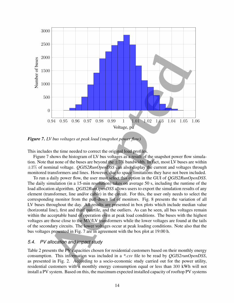
Acce
pted094 095 096 097 098 099 1 101 102 103 104 105 106
0
500
1000
1500
2000
2500
3000
Voltage pu
Num
bero
fbus
es
Figure 7 LV bus voltages at peak load (snapshot power flow)
This includes the time needed to correct the original load profilesFigure 7 shows the histogram of LV bus voltages as a result of the snapshot power flow simula-
tion Note that none of the buses are beyond theplusmn5 bandwidth In fact most LV buses are withinplusmn3 of nominal voltage QGIS2RunOpenDSS can also display the current and voltages throughmonitored transformers and lines However due to space limitations they have not been included
To run a daily power flow the user must select this option in the GUI of QGIS2RunOpenDSSThe daily simulation (in a 15-min resolution) takes on average 50 s including the runtime of theload allocation algorithm QGIS2RunOpenDSS allows users to export the simulation results of anyelement (transformer line andor cable) in the circuit For this the user only needs to select thecorresponding monitor from the pull-down list of monitors Fig 8 presents the variation of allLV buses throughout the day All results are presented in box plots which include median value(horizontal line) first and third quartile and the outliers As can be seen all bus voltages remainwithin the acceptable band of operation even at peak load conditions The buses with the highestvoltages are those close to the MVLV transformers while the lower voltages are found at the tailsof the secondary circuits The lower voltages occur at peak loading conditions Note also that thebus voltages presented in Fig 7 are in agreement with the box plot at 1900 h
54 PV allocation and impact study
Table 2 presents the PV capacities chosen for residential customers based on their monthly energyconsumption This information was included in a csv file to be read by QGIS2runOpenDSSas presented in Fig 2 According to a socio-economic study carried out for the power utilityresidential customers with a monthly energy consumption equal or less than 300 kWh will notinstall a PV system Based on this the maximum expected installed capacity of rooftop PV systems
14
Acce
pted0000 0300 0600 0900 1200 1500 1800 2100 0000
095
1
105
Volta
gep
u
Time
Figure 8 LV bus voltages through out the day (daily power flow)
Table 2 Information required by plugin to assign the PV systems
Monthly consumption (kWh) Capacity (kW)gt 300 000
300 - 320 075330 - 360 100370 - 380 125390 - 680 325690 - 950 525
is 1700 kW throughout the circuitThe plugin randomly allocates these PV systems among the customers until the requested pen-
etration level is met Figure 9 presents the simulation result of the active power demand when the1700 kW are installed in the circuit When compared to the base case it is seen that the circuitdemanded less power from 600 to 1800 h This small penetration level is not expected to largelyaffect the operation of the network
Although not shown here the voltages increased during the day thanks to the active powerinjection of rooftop PV systems when compared to the base case
6 Discussion
As demonstrated before detailed studies of future DNs with LCTs will be easily carried out thanksto the integration of GIS and advanced simulation tools such as OpenDSS In addition results ofsocio-economic studies can help to simulate more realistic scenarios These tools could also beextended to assess the network condition in the presence of PV and energy storage systems alongwith irradiation layers to better represent the solar potential at a given geographic area In addition
15
Acce
pted0000 0300 0600 0900 1200 1500 1800 2100 0000
6
8
10
12
14
16
18
Time
Dem
and
MW
0 kW1700 kW
Figure 9 Feederrsquos load profile with PVs
the integration of transportation layers could also be used when studying the integration of ElectricVehicles (EVs) into the grid and the optimal location of fast charging stations
The key to carry out these studies is high quality GIS data This information needs to becleaned from spurious data that could result in unrealistic engineering network models Indeedthe correction of errors is not straightforward and requires knowledge of how GIS network modelsare built and how they have to be translated for power engineering uses
From authors experience most errors are found in secondary systems due to the presence ofmany short line segments and also because LV systems were not included in traditional studies runby power utilities To overcome this the aforementioned tools should be complemented with newplugins able to automatically correct frequently found errors such as disconnected LV elements ornonexistent connections among different secondary circuits For example Kd-tree could be used toautomatically identify service cables inside a circle centered at the disconnected load If a servicecable was found inside the circle the coordinate of the disconnected load should be corrected tomatch the coordinate of the service cable end Similar procedure could be carried out to connectline segments Unfortunately not all disconnection problems will be automatically corrected assome cases require human intervention to decide where to connect a disconnected element
The identification of connected elements is likely to be the most important step when buildingthe engineering model in OpenDSS As reported in Section 32 this task was successfully achievedthanks to the Kd-tree algorithm However the authors believe that the same task could be accom-plished by more efficient computational tools based on Graph theory In this regard future workwill focus on reducing the time requirements for the connectivity of network elements
To take full advantages of GIS software capabilities future work will also be focused on vi-sualization of simulation results This is the simulation results currently shown in plots will be
16
Acce
pted
visualized in the GIS network model For instance overvoltages due to massive integration ofPVs or under voltages caused by high EV penetrations at LV level could be represented in theGIS environment by heatmaps or different scale colors In addition some GIS properties of DNelements could be also modified (eg line thickness or point size) to represent highly loaded oreven overloaded lines and transformers
Finally detailed simulations of smart distribution networks will be further improved when loadprofiles from smart meters replace the typical profiles currently used by the developed tools Thiswill also require the integration of databases fed from smart meters with the QGIS software
7 Conclusion
This paper has presented the integration of OpenDSS with an open source GIS platform to carryout easier and more efficient studies of distribution networks Two software plugins were created toextract GIS data to automatically build a distribution network engineering model and run OpenDSSas an embedded tool in the GIS platform These plugins aim at facilitating the studies that powerengineers have to run in the short term by integrating free and open source GIS software withexisting free and open source power engineering software In addition they have great potential tobe used for educational purposes at university level and for training of junior engineers
The performance of the simulation tool has been demonstrated on a real circuit in Costa Ricawith more than 10000 customers The illustrative examples highlight the efficiency and conve-nience of the tool to perform detailed network studies
The release of these tools is expected to bring new opportunities to power utilities researchlaboratories and universities to test and simulate novel smart grid solutions with more realisticnetwork models In addition future collaborations from other users will enhance the robustnessand generality of the tools
8 Acknowledgment
The authors would like to thank CNFL for providing the GIS database of the analyzed circuit
9 References
[1] R Arritt and R Dugan ldquoDistribution System Analysis and the Future Smart Gridrdquo IEEETransactions on Industry Applications vol 47 no 6 pp 2343ndash2350 Nov 2011
[2] G Shirek B A Lassiter W Carr and W H Kersting ldquoModeling Secondary Services inEngineering and Mappingrdquo IEEE Transactions on Industry Applications vol 48 no 1 pp254ndash262 Feb 2012
[3] A Navarro-Espinosa L Ochoa R Shaw and D Randles ldquoReconstruction of Low Volt-age Distribution Networks From GIS Data to Power Flow Modelsrdquo in 23rd InternationalConference on Electricity Distribution no 1273 CIRED 2015
[4] B Meehan GIS for Enhanced Electric Utility Performance Artech House 2013
[5] R Brenes A Arguello J Quiros-Tortos and G Valverde ldquoDistribution Network ElementModel Parameters Creation of Databaserdquo in IEEE CONCAPAN Nov 2016
17
Acce
pted
[6] A Crossland N Wade and D Jones ldquoExtraction of 9163 Real LV Network Models fromDNO GIS Database to Assess Overvoltage from PV and Consequent Mitigation Measuresrdquoin 23rd International Conference on Electricity Distribution no 0915 CIRED 2015
[7] S Lazarou V Vita P Karampelas and L Ekonomou ldquoA Power System Simulation Platformfor Planning and Evaluating Distributed Generation Systems based on GISrdquo Energy Systemsvol 4 no 4 pp 379ndash391 Apr 2013
[8] F Milano Power System Modelling and Scripting Springer 2010
[9] R Dugan and T E McDermott ldquoAn Open Source Platform for Collaborating on Smart GridResearchrdquo in IEEE PES General Meeting 2011
[10] D P Chassin K Schneider and C Gerkensmeyer ldquoGridLAB-D An Open-Source PowerSystems Modeling and Simulation Environmentrdquo in 2008 IEEEPES Transmission and Dis-tribution Conference and Exposition April 2008 pp 1ndash5
[11] EPERLab ldquoRelease of plugins Integration of Open Source Tools for StudyingLarge-Scale Distribution Networksrdquo 2017 [Online] Available httpeperlabeieucraccrdocuments [Available from Jul 2017]
[12] Task Force on Open Source Software for Power Systems Open Source Software IEEEPSACE Committee [Online] Available httpewhieeeorgcmtepsaceCAMS taskforcesoftwarehtm
[13] P Bolstad GIS Fundementals a First Text on Geographical Information Systems 4th edMinnesota EEUU Eider Press 2002
[14] QGIS PyQGIS Developer Cookbook February 2016 [Online] Available httpdocsqgisorg
[15] R Dugan Reference Guide The Open Distribution System Simulator EPRI June 2013
[16] W H Kersting Distribution System Modeling and Analysis 3rd ed CRC Press 2012
[17] T Short Electric Power Distribution Handbook CRC 2004
[18] J L Bentley ldquoMultidimensional Binary Search Trees Used for Associative Searchingrdquo Com-munications of the ACM vol 18 no 9 pp 509ndash517 Sept 1975
[19] J Quiros-Tortos A Arguello and G Valverde ldquoStatistical Analysis of Residential DemandBehavior in Costa Rica Creation of Load Profilesrdquo in IEEE CONCAPAN Nov 2016
18
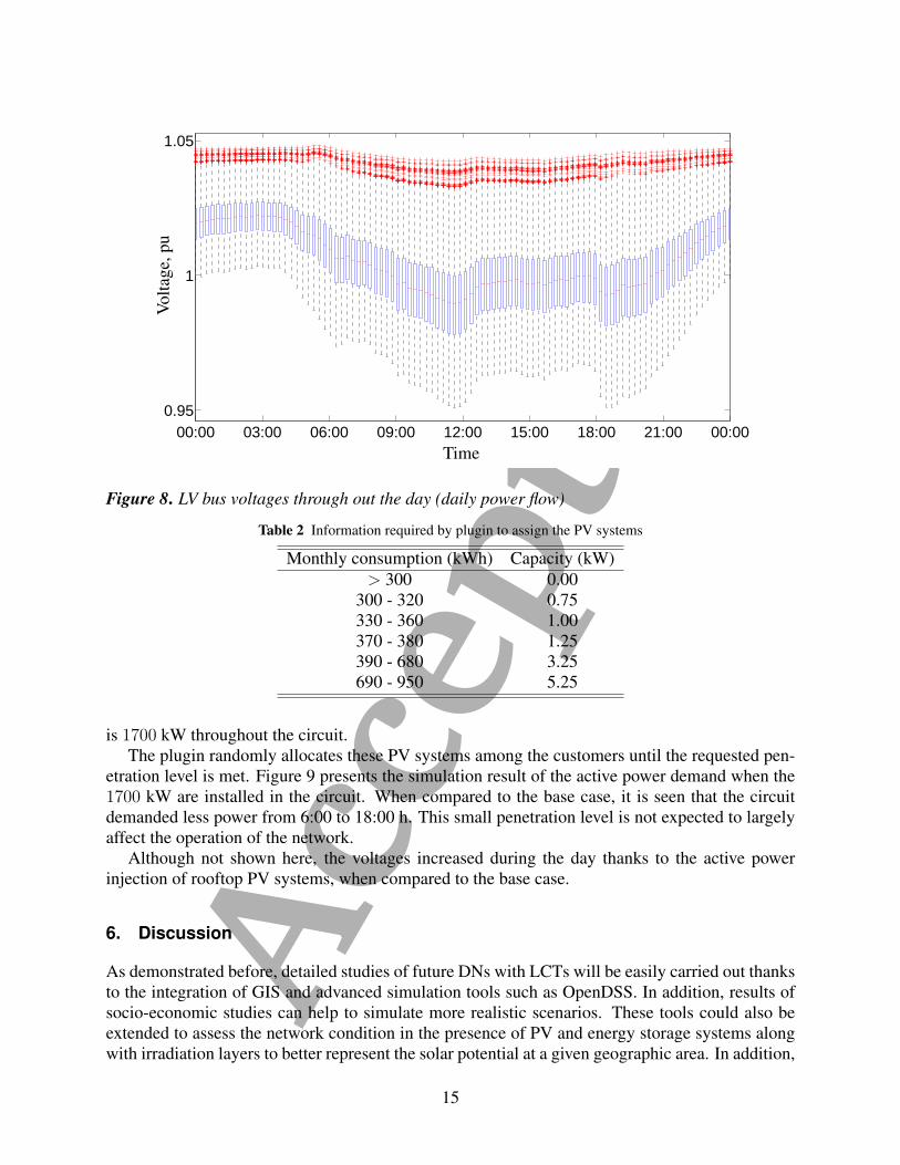
Acce
pted0000 0300 0600 0900 1200 1500 1800 2100 0000
095
1
105
Volta
gep
u
Time
Figure 8 LV bus voltages through out the day (daily power flow)
Table 2 Information required by plugin to assign the PV systems
Monthly consumption (kWh) Capacity (kW)gt 300 000
300 - 320 075330 - 360 100370 - 380 125390 - 680 325690 - 950 525
is 1700 kW throughout the circuitThe plugin randomly allocates these PV systems among the customers until the requested pen-
etration level is met Figure 9 presents the simulation result of the active power demand when the1700 kW are installed in the circuit When compared to the base case it is seen that the circuitdemanded less power from 600 to 1800 h This small penetration level is not expected to largelyaffect the operation of the network
Although not shown here the voltages increased during the day thanks to the active powerinjection of rooftop PV systems when compared to the base case
6 Discussion
As demonstrated before detailed studies of future DNs with LCTs will be easily carried out thanksto the integration of GIS and advanced simulation tools such as OpenDSS In addition results ofsocio-economic studies can help to simulate more realistic scenarios These tools could also beextended to assess the network condition in the presence of PV and energy storage systems alongwith irradiation layers to better represent the solar potential at a given geographic area In addition
15
Acce
pted0000 0300 0600 0900 1200 1500 1800 2100 0000
6
8
10
12
14
16
18
Time
Dem
and
MW
0 kW1700 kW
Figure 9 Feederrsquos load profile with PVs
the integration of transportation layers could also be used when studying the integration of ElectricVehicles (EVs) into the grid and the optimal location of fast charging stations
The key to carry out these studies is high quality GIS data This information needs to becleaned from spurious data that could result in unrealistic engineering network models Indeedthe correction of errors is not straightforward and requires knowledge of how GIS network modelsare built and how they have to be translated for power engineering uses
From authors experience most errors are found in secondary systems due to the presence ofmany short line segments and also because LV systems were not included in traditional studies runby power utilities To overcome this the aforementioned tools should be complemented with newplugins able to automatically correct frequently found errors such as disconnected LV elements ornonexistent connections among different secondary circuits For example Kd-tree could be used toautomatically identify service cables inside a circle centered at the disconnected load If a servicecable was found inside the circle the coordinate of the disconnected load should be corrected tomatch the coordinate of the service cable end Similar procedure could be carried out to connectline segments Unfortunately not all disconnection problems will be automatically corrected assome cases require human intervention to decide where to connect a disconnected element
The identification of connected elements is likely to be the most important step when buildingthe engineering model in OpenDSS As reported in Section 32 this task was successfully achievedthanks to the Kd-tree algorithm However the authors believe that the same task could be accom-plished by more efficient computational tools based on Graph theory In this regard future workwill focus on reducing the time requirements for the connectivity of network elements
To take full advantages of GIS software capabilities future work will also be focused on vi-sualization of simulation results This is the simulation results currently shown in plots will be
16
Acce
pted
visualized in the GIS network model For instance overvoltages due to massive integration ofPVs or under voltages caused by high EV penetrations at LV level could be represented in theGIS environment by heatmaps or different scale colors In addition some GIS properties of DNelements could be also modified (eg line thickness or point size) to represent highly loaded oreven overloaded lines and transformers
Finally detailed simulations of smart distribution networks will be further improved when loadprofiles from smart meters replace the typical profiles currently used by the developed tools Thiswill also require the integration of databases fed from smart meters with the QGIS software
7 Conclusion
This paper has presented the integration of OpenDSS with an open source GIS platform to carryout easier and more efficient studies of distribution networks Two software plugins were created toextract GIS data to automatically build a distribution network engineering model and run OpenDSSas an embedded tool in the GIS platform These plugins aim at facilitating the studies that powerengineers have to run in the short term by integrating free and open source GIS software withexisting free and open source power engineering software In addition they have great potential tobe used for educational purposes at university level and for training of junior engineers
The performance of the simulation tool has been demonstrated on a real circuit in Costa Ricawith more than 10000 customers The illustrative examples highlight the efficiency and conve-nience of the tool to perform detailed network studies
The release of these tools is expected to bring new opportunities to power utilities researchlaboratories and universities to test and simulate novel smart grid solutions with more realisticnetwork models In addition future collaborations from other users will enhance the robustnessand generality of the tools
8 Acknowledgment
The authors would like to thank CNFL for providing the GIS database of the analyzed circuit
9 References
[1] R Arritt and R Dugan ldquoDistribution System Analysis and the Future Smart Gridrdquo IEEETransactions on Industry Applications vol 47 no 6 pp 2343ndash2350 Nov 2011
[2] G Shirek B A Lassiter W Carr and W H Kersting ldquoModeling Secondary Services inEngineering and Mappingrdquo IEEE Transactions on Industry Applications vol 48 no 1 pp254ndash262 Feb 2012
[3] A Navarro-Espinosa L Ochoa R Shaw and D Randles ldquoReconstruction of Low Volt-age Distribution Networks From GIS Data to Power Flow Modelsrdquo in 23rd InternationalConference on Electricity Distribution no 1273 CIRED 2015
[4] B Meehan GIS for Enhanced Electric Utility Performance Artech House 2013
[5] R Brenes A Arguello J Quiros-Tortos and G Valverde ldquoDistribution Network ElementModel Parameters Creation of Databaserdquo in IEEE CONCAPAN Nov 2016
17
Acce
pted
[6] A Crossland N Wade and D Jones ldquoExtraction of 9163 Real LV Network Models fromDNO GIS Database to Assess Overvoltage from PV and Consequent Mitigation Measuresrdquoin 23rd International Conference on Electricity Distribution no 0915 CIRED 2015
[7] S Lazarou V Vita P Karampelas and L Ekonomou ldquoA Power System Simulation Platformfor Planning and Evaluating Distributed Generation Systems based on GISrdquo Energy Systemsvol 4 no 4 pp 379ndash391 Apr 2013
[8] F Milano Power System Modelling and Scripting Springer 2010
[9] R Dugan and T E McDermott ldquoAn Open Source Platform for Collaborating on Smart GridResearchrdquo in IEEE PES General Meeting 2011
[10] D P Chassin K Schneider and C Gerkensmeyer ldquoGridLAB-D An Open-Source PowerSystems Modeling and Simulation Environmentrdquo in 2008 IEEEPES Transmission and Dis-tribution Conference and Exposition April 2008 pp 1ndash5
[11] EPERLab ldquoRelease of plugins Integration of Open Source Tools for StudyingLarge-Scale Distribution Networksrdquo 2017 [Online] Available httpeperlabeieucraccrdocuments [Available from Jul 2017]
[12] Task Force on Open Source Software for Power Systems Open Source Software IEEEPSACE Committee [Online] Available httpewhieeeorgcmtepsaceCAMS taskforcesoftwarehtm
[13] P Bolstad GIS Fundementals a First Text on Geographical Information Systems 4th edMinnesota EEUU Eider Press 2002
[14] QGIS PyQGIS Developer Cookbook February 2016 [Online] Available httpdocsqgisorg
[15] R Dugan Reference Guide The Open Distribution System Simulator EPRI June 2013
[16] W H Kersting Distribution System Modeling and Analysis 3rd ed CRC Press 2012
[17] T Short Electric Power Distribution Handbook CRC 2004
[18] J L Bentley ldquoMultidimensional Binary Search Trees Used for Associative Searchingrdquo Com-munications of the ACM vol 18 no 9 pp 509ndash517 Sept 1975
[19] J Quiros-Tortos A Arguello and G Valverde ldquoStatistical Analysis of Residential DemandBehavior in Costa Rica Creation of Load Profilesrdquo in IEEE CONCAPAN Nov 2016
18
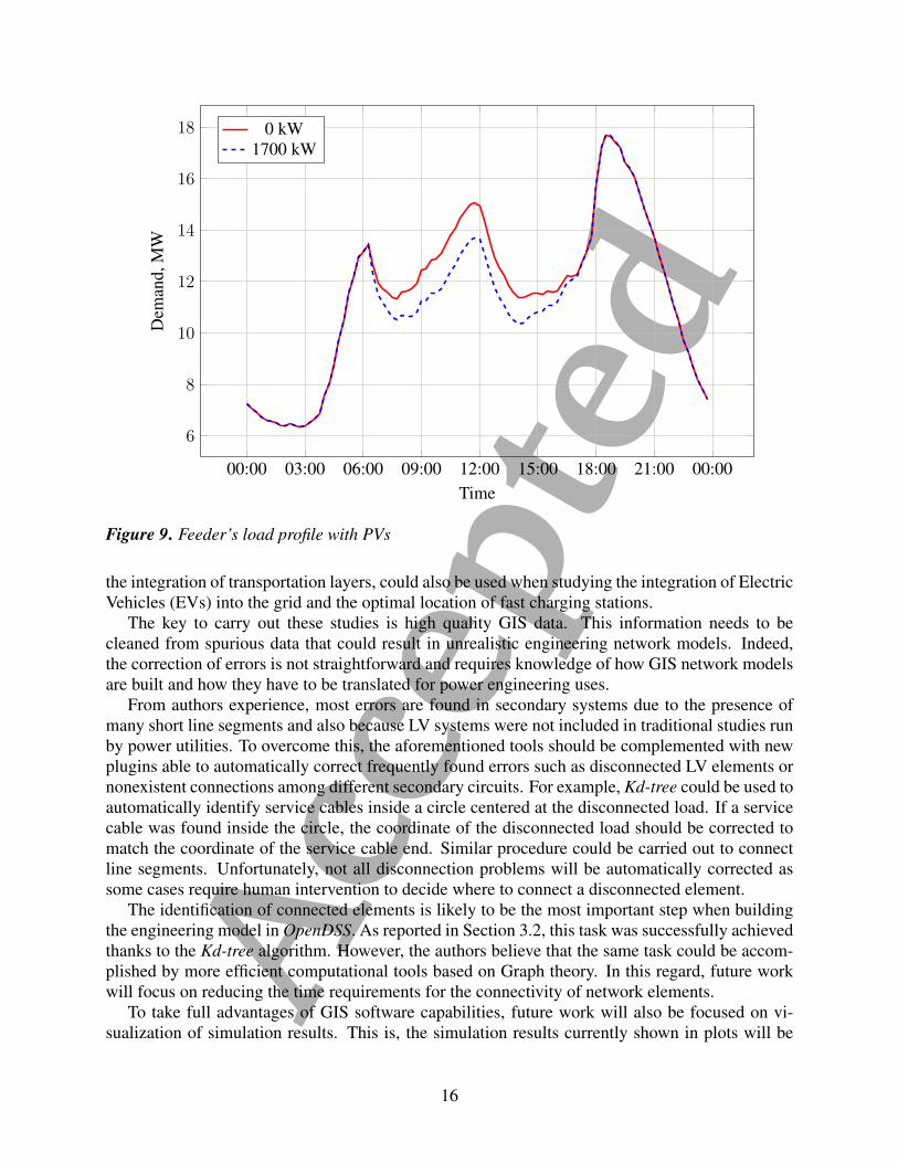
Acce
pted0000 0300 0600 0900 1200 1500 1800 2100 0000
6
8
10
12
14
16
18
Time
Dem
and
MW
0 kW1700 kW
Figure 9 Feederrsquos load profile with PVs
the integration of transportation layers could also be used when studying the integration of ElectricVehicles (EVs) into the grid and the optimal location of fast charging stations
The key to carry out these studies is high quality GIS data This information needs to becleaned from spurious data that could result in unrealistic engineering network models Indeedthe correction of errors is not straightforward and requires knowledge of how GIS network modelsare built and how they have to be translated for power engineering uses
From authors experience most errors are found in secondary systems due to the presence ofmany short line segments and also because LV systems were not included in traditional studies runby power utilities To overcome this the aforementioned tools should be complemented with newplugins able to automatically correct frequently found errors such as disconnected LV elements ornonexistent connections among different secondary circuits For example Kd-tree could be used toautomatically identify service cables inside a circle centered at the disconnected load If a servicecable was found inside the circle the coordinate of the disconnected load should be corrected tomatch the coordinate of the service cable end Similar procedure could be carried out to connectline segments Unfortunately not all disconnection problems will be automatically corrected assome cases require human intervention to decide where to connect a disconnected element
The identification of connected elements is likely to be the most important step when buildingthe engineering model in OpenDSS As reported in Section 32 this task was successfully achievedthanks to the Kd-tree algorithm However the authors believe that the same task could be accom-plished by more efficient computational tools based on Graph theory In this regard future workwill focus on reducing the time requirements for the connectivity of network elements
To take full advantages of GIS software capabilities future work will also be focused on vi-sualization of simulation results This is the simulation results currently shown in plots will be
16
Acce
pted
visualized in the GIS network model For instance overvoltages due to massive integration ofPVs or under voltages caused by high EV penetrations at LV level could be represented in theGIS environment by heatmaps or different scale colors In addition some GIS properties of DNelements could be also modified (eg line thickness or point size) to represent highly loaded oreven overloaded lines and transformers
Finally detailed simulations of smart distribution networks will be further improved when loadprofiles from smart meters replace the typical profiles currently used by the developed tools Thiswill also require the integration of databases fed from smart meters with the QGIS software
7 Conclusion
This paper has presented the integration of OpenDSS with an open source GIS platform to carryout easier and more efficient studies of distribution networks Two software plugins were created toextract GIS data to automatically build a distribution network engineering model and run OpenDSSas an embedded tool in the GIS platform These plugins aim at facilitating the studies that powerengineers have to run in the short term by integrating free and open source GIS software withexisting free and open source power engineering software In addition they have great potential tobe used for educational purposes at university level and for training of junior engineers
The performance of the simulation tool has been demonstrated on a real circuit in Costa Ricawith more than 10000 customers The illustrative examples highlight the efficiency and conve-nience of the tool to perform detailed network studies
The release of these tools is expected to bring new opportunities to power utilities researchlaboratories and universities to test and simulate novel smart grid solutions with more realisticnetwork models In addition future collaborations from other users will enhance the robustnessand generality of the tools
8 Acknowledgment
The authors would like to thank CNFL for providing the GIS database of the analyzed circuit
9 References
[1] R Arritt and R Dugan ldquoDistribution System Analysis and the Future Smart Gridrdquo IEEETransactions on Industry Applications vol 47 no 6 pp 2343ndash2350 Nov 2011
[2] G Shirek B A Lassiter W Carr and W H Kersting ldquoModeling Secondary Services inEngineering and Mappingrdquo IEEE Transactions on Industry Applications vol 48 no 1 pp254ndash262 Feb 2012
[3] A Navarro-Espinosa L Ochoa R Shaw and D Randles ldquoReconstruction of Low Volt-age Distribution Networks From GIS Data to Power Flow Modelsrdquo in 23rd InternationalConference on Electricity Distribution no 1273 CIRED 2015
[4] B Meehan GIS for Enhanced Electric Utility Performance Artech House 2013
[5] R Brenes A Arguello J Quiros-Tortos and G Valverde ldquoDistribution Network ElementModel Parameters Creation of Databaserdquo in IEEE CONCAPAN Nov 2016
17
Acce
pted
[6] A Crossland N Wade and D Jones ldquoExtraction of 9163 Real LV Network Models fromDNO GIS Database to Assess Overvoltage from PV and Consequent Mitigation Measuresrdquoin 23rd International Conference on Electricity Distribution no 0915 CIRED 2015
[7] S Lazarou V Vita P Karampelas and L Ekonomou ldquoA Power System Simulation Platformfor Planning and Evaluating Distributed Generation Systems based on GISrdquo Energy Systemsvol 4 no 4 pp 379ndash391 Apr 2013
[8] F Milano Power System Modelling and Scripting Springer 2010
[9] R Dugan and T E McDermott ldquoAn Open Source Platform for Collaborating on Smart GridResearchrdquo in IEEE PES General Meeting 2011
[10] D P Chassin K Schneider and C Gerkensmeyer ldquoGridLAB-D An Open-Source PowerSystems Modeling and Simulation Environmentrdquo in 2008 IEEEPES Transmission and Dis-tribution Conference and Exposition April 2008 pp 1ndash5
[11] EPERLab ldquoRelease of plugins Integration of Open Source Tools for StudyingLarge-Scale Distribution Networksrdquo 2017 [Online] Available httpeperlabeieucraccrdocuments [Available from Jul 2017]
[12] Task Force on Open Source Software for Power Systems Open Source Software IEEEPSACE Committee [Online] Available httpewhieeeorgcmtepsaceCAMS taskforcesoftwarehtm
[13] P Bolstad GIS Fundementals a First Text on Geographical Information Systems 4th edMinnesota EEUU Eider Press 2002
[14] QGIS PyQGIS Developer Cookbook February 2016 [Online] Available httpdocsqgisorg
[15] R Dugan Reference Guide The Open Distribution System Simulator EPRI June 2013
[16] W H Kersting Distribution System Modeling and Analysis 3rd ed CRC Press 2012
[17] T Short Electric Power Distribution Handbook CRC 2004
[18] J L Bentley ldquoMultidimensional Binary Search Trees Used for Associative Searchingrdquo Com-munications of the ACM vol 18 no 9 pp 509ndash517 Sept 1975
[19] J Quiros-Tortos A Arguello and G Valverde ldquoStatistical Analysis of Residential DemandBehavior in Costa Rica Creation of Load Profilesrdquo in IEEE CONCAPAN Nov 2016
18

Acce
pted
[6] A Crossland N Wade and D Jones ldquoExtraction of 9163 Real LV Network Models fromDNO GIS Database to Assess Overvoltage from PV and Consequent Mitigation Measuresrdquoin 23rd International Conference on Electricity Distribution no 0915 CIRED 2015
[7] S Lazarou V Vita P Karampelas and L Ekonomou ldquoA Power System Simulation Platformfor Planning and Evaluating Distributed Generation Systems based on GISrdquo Energy Systemsvol 4 no 4 pp 379ndash391 Apr 2013
[8] F Milano Power System Modelling and Scripting Springer 2010
[9] R Dugan and T E McDermott ldquoAn Open Source Platform for Collaborating on Smart GridResearchrdquo in IEEE PES General Meeting 2011
[10] D P Chassin K Schneider and C Gerkensmeyer ldquoGridLAB-D An Open-Source PowerSystems Modeling and Simulation Environmentrdquo in 2008 IEEEPES Transmission and Dis-tribution Conference and Exposition April 2008 pp 1ndash5
[11] EPERLab ldquoRelease of plugins Integration of Open Source Tools for StudyingLarge-Scale Distribution Networksrdquo 2017 [Online] Available httpeperlabeieucraccrdocuments [Available from Jul 2017]
[12] Task Force on Open Source Software for Power Systems Open Source Software IEEEPSACE Committee [Online] Available httpewhieeeorgcmtepsaceCAMS taskforcesoftwarehtm
[13] P Bolstad GIS Fundementals a First Text on Geographical Information Systems 4th edMinnesota EEUU Eider Press 2002
[14] QGIS PyQGIS Developer Cookbook February 2016 [Online] Available httpdocsqgisorg
[15] R Dugan Reference Guide The Open Distribution System Simulator EPRI June 2013
[16] W H Kersting Distribution System Modeling and Analysis 3rd ed CRC Press 2012
[17] T Short Electric Power Distribution Handbook CRC 2004
[18] J L Bentley ldquoMultidimensional Binary Search Trees Used for Associative Searchingrdquo Com-munications of the ACM vol 18 no 9 pp 509ndash517 Sept 1975
[19] J Quiros-Tortos A Arguello and G Valverde ldquoStatistical Analysis of Residential DemandBehavior in Costa Rica Creation of Load Profilesrdquo in IEEE CONCAPAN Nov 2016
18


![Definisikan Litar Bersepadu. [2 marks] [2 markah] (b) Identify the differences between Small Scale Integration (SSI), Medium Scale Integration (MSI) and Large Scale Integration](https://img.pdfslide.us/doc/110x75/5e6386966d732830c31007f0/-definisikan-litar-bersepadu-2-marks-2-markah-b-identify-the-differences.jpg)