arX

iv:1

302.

0651

v1 [

phys

ics.

atom

-ph]

4 F

eb 2

013

Multiphoton ionization of the Calcium atom by linearly and

circularly polarized laser fields

Gabriela Buica

Institute for Space Sciences, P.O. Box MG-23,

Ro 77125, Bucharest-Magurele, Romania

Takashi Nakajima∗

Institute of Advanced Energy, Kyoto University,

Gokasho, Uji, Kyoto 611-0011, Japan

Abstract

We theoretically study multiphoton ionization of the Ca atom irradiated by the second (photon

energy 3.1 eV) and third (photon energy 4.65 eV) harmonics of Ti:sapphire laser pulses (photon

energy 1.55 eV). Because of the dense energy level structure the second and third harmonics of

a Ti:sapphire laser are nearly single-photon resonant with the 4s4p 1P o and 4s5p 1P o states,

respectively. Although two-photon ionization takes place through the near-resonant intermediate

states with the same symmetry in both cases, it turns out that there are significant differences

between them. The photoelectron energy spectra exhibit the absence/presence of substructures.

More interestingly, the photoelectron angular distributions clearly show that the main contribution

to the ionization processes by the third harmonic arises from the far off-resonant 4s4p 1P o state

rather than the near-resonant 4s5p 1P o state. These findings can be attributed to the fact that

the dipole moment for the 4s2 1Se - 4s5p 1P o transition is much smaller than that for the 4s2 1Se

- 4s4p 1P o transition.

PACS numbers: 32.80.Rm, 42.50.Hz

Keywords:

∗t-nakajima@iae.kyoto-u.ac.jp

1

I. INTRODUCTION

Above-threshold ionization (ATI) [1] is a process in which atoms absorb more than the

minimum number of photons required to ionize and the photoelectron energy spectrum

(PES) consists of a series of peaks that are equally separated by the photon energy. Now

the ATI and multiphoton ionization (MPI) processes have been well-studied [2, 3], especially

for rare gas atoms. Recently, we have presented several new interesting features in the PES

of a light alkaline-earth-metal atom, Mg, interacting with a short laser pulse [4, 5]. We

have had a close look at the intermediate ATI peaks appearing in the PES and clarified

their origin as the off-resonant excitation of the bound states. In this paper we extend our

previous works on Mg to another alkaline-earth-metal atom which is less investigated in the

literature, the Ca atom.

During the last 30 years many theoretical and experimental investigations have been

performed for Ca to obtain the atomic data and to understand its interaction with laser

fields for the single-photon processes. The first extensive theoretical studies for the singlet

series 1S and 1P of Ca were performed by Fischer and Hansen [6] with a multi-configuration

Hartree-Fock (MCFH) method which included correlations between the valence electrons.

Later on, Mitroy [7] calculated the energy level and oscillator strength (OS) for the low-

lying levels of Ca using the frozen-core Hartree-Fock (FCHF) approach including a model

potential. Aymar and co-workers [8] extensively studied light alkaline-earth-metal atoms

using the multichannel quantum defect theory and eigenchannel R-matrix combined with

polarization potentials. Hansen and co-workers [9] used a configuration interaction (CI)

approach, based on the B-spline basis functions and a model potential with dielectronic

core polarization potential, to calculate term energies and wave functions for the singlet and

triplet states of Ca. Recently, Fischer and Tachiev [10] calculated the energy levels, transition

probabilities, and lifetimes for the singlet and triplet spectra of Ca using the MCFH method

with lowest-order relativistic effects included through a Breit-Pauli Hamiltonian.

As for the MPI processes Benec’h and Bachau [11] calculated the one-, two-, and three-

photon ionization cross sections of Ca from the ground state with B-spline basis functions

and CI procedure, where the FCHF approach and polarization potentials were employed to

construct the atomic basis. Regarding the experimental MPI processes of Ca, there are only

several works in the literature, all of which involve only ns and ps laser pulses. DiMauro and

2

co-workers [12] investigated single and double ionization of Ca by 10 ns Nd:YAG laser pulses

at 532 and 1064 nm in the intensity range of 1010 − 1013W/cm2. Shao and co-workers [13]

analyzed single and double ionization of Ca by 35 and 200 ps Nd:YAG laser pulses at 532

and 1064 nm in the intensity range of 1010−2×1013 W/cm2. Lately, Cohen and co-workers

[14] experimentally and theoretically studied the two-photon ionization spectra of Ca in the

374-323 nm wavelength range with a ∼5 ns dye laser. Although theoretical data for MPI of

alkaline-earth-metal atoms such as Ca by fs laser pulses would provide additional valuable

information for the purpose of understanding the multiphoton ionization dynamics, such

data are still missing in the literature.

The aim of this work is to extend our previous investigations for MPI of Mg [4, 5, 15, 16]

to the Ca atom: In this paper we study the MPI processes of Ca by the second (photon

energy 3.1 eV) and third (photon energy 4.65 eV) harmonics of Ti:sapphire laser pulses.

For this purpose we use a nonperturbative method to solve the time-dependent Schrodinger

equation (TDSE) with two active electrons. In Sec. II we construct an atomic basis set in

terms of discretized states and use it in Sec. III to numerically solve the TDSE. Numerical

results such as the ionization yields, PES, and photoelectron angular distribution (PAD) are

presented in in Sec. IV. Atomic units (a.u.) are used throughout this paper unless otherwise

mentioned.

II. ATOMIC BASIS STATES

The Ca atom is a two-valence-electron atom with a closed ionic core Ca2+ (the nucleus

and the 18 inner-shell electrons 1s22s22p63s23p6) and the two valence electrons, 4s2 1Se.

Since it is a heavier alkaline-earth-metal element than Be and Mg and hence the core, Ca2+,

is softer, there are more complexities as well as subtleties in the Ca atomic structure. As it

is already mentioned in the literature [17, 18] there are several different approaches to solve

the Schrodinger equation to describe the interaction of a one- and two-valence-electron atom

with a laser field. Since the general computational procedure has already been presented

in Refs. [5, 16, 19–21] and the specific details about the atomic structure calculation of

Ca have been reported in recent works [9, 11, 22], we only make a brief description of the

method we employ. The field-free one-electron Hamiltonian of Ca+, Ha(r), is expressed as:

Ha(r) = −1

2

d2

dr2−

Z

r+

l(l + 1)

2r2+ Veff (r), (1)

3

where Veff(r) is the effective potential acting on the valence electron of Ca+, r represents

the position vector of the valence electron, Z is the electric charge of the core (Z = 2 for

a two-valence-electron atom), and l is the orbital quantum number. In our approach the

effective potential, Veff (r), consists of the FCHF potential (FCHFP) and the additional

core-polarization potential which will be introduced in the next subsection.

A. One-Electron Orbitals: Frozen-Core Hartree-Fock approach

To describe the ionic core Ca2+ we have introduced the effective potential in Eq. (1),

which is a sum of the FCHFP, V HFl (r), and the core-polarization potential, V p

l (r, αs, rl):

Veff(r) = V HFl (r) + V p

l (r, αs, rl). (2)

V pl (r, αs, rl) describes the interaction between the ionic core and the valence electrons and

can be written in the form of

V pl (r, αs, rl) = −

αs

2r4

[

1− exp−(r/rl)6]

, (3)

where αs is the static dipole polarizability of Ca2+ and rl the cutoff radii for the different

orbital angular momenta, l = 0, 1, 2, ..., etc [19]. The values of rl have been obtained by

performing the fittings of the one-electron energies to their experimental values [23] for the

four lowest states of s, p, d and f series of Ca+. We have used the following set of cutoff

radii, r0 = 1.5457, r1 = 1.5857, r2 = 1.8771, and rl≥3 = 1.5530 together with the static

dipole polarizability of Ca2+ which is αs = 3.16 [24]. The relatively large value of the cutoff

radius for l = 2 is due to the fact the 3d orbital penetrates the ionic core much more than

the other orbitals, and therefore the core-polarization potential is more sensitive for the

l = 2 orbital than for other orbitals. We note that other theoretical papers [7–9, 11, 22] use

slightly different values for the static dipole polarizability and cutoff radii.

With the aid of the mathematical properties of the B-spline polynomials [18, 19] to

expand the one-electron orbitals, solving the one-electron Schrodinger equation for the non-

relativistic one-electron Hamiltonian given by Eq. (1) is now equivalent to an eigenvalue

problem.

4

B. Two-electron states

The field-free two-electron Hamiltonian, Ha(r1, r2), can be expressed as

Ha(r1, r2) =2

∑

i=1

Ha(ri) + V (r1, r2), (4)

where Ha(ri) represents the one-electron Hamiltonian for the ith electron as shown in Eq.

(1), and V (r1, r2) is a two-electron interaction operator which includes the static Coulomb

interaction 1/|r1 − r2| and the effective dielectronic interaction potential [19, 25]. Here

r1 and r2 are the position vectors of the two valence electrons. To solve the two-electron

Schrodinger equation for the Hamiltonian given in Eq. (4) the two-electron states can be

constructed within the CI approach. Namely, we use a linear combination of the products

of the two one-electron orbitals to represent a two-electron states and diagonalize the two-

electron Hamiltonian given in Eq.(4). This is so-called a CI procedure [19–21].

For Ca, which is heavier than Be and Mg but still relatively light alkaline-earth-metal

atom, the LS coupling is known to give a fair description [7–9, 11] and hence it is sufficient

to label a two-electron state by the following set of quantum numbers: principal, orbital,

and spin quantum numbers for each electron, nilisi (i = 1, 2), total orbital momentum L,

total spin S, total angular momentum J , and its projection M on the quantization axis.

After the CI procedure the two-electron states may be most generally labeled by the state

energy and the quantum numbers (L, S, J,M), and furthermore the above state labeling can

be simplified to (L,M) for singlet states (S = 0). Having obtained the two-electron wave

functions we can calculate the dipole matrix elements as well as OSs for both LP and CP

laser pulses.

III. TIME-DEPENDENT SCHRODINGER EQUATION

By making use of the two-electron states which have been constructed in Sec. II, we can

solve the TDSE for the two-electron atom interacting with a laser pulse. The TDSE reads

i∂

∂tΨ(r1, r2; t) = [Ha(r1, r2) +D(t)]Ψ(r1, r2; t), (5)

where Ψ(r1, r2; t) is the two-electron wave function for the two electrons located at r1 and

r2 at time t, and Ha(r1, r2) is the field-free two-electron Hamiltonian shown in Eq. (4). The

5

time-dependent interaction operator, D(t), between the atom and the laser pulse is written

in the velocity gauge and dipole approximation as,

D(t) = −A(t) · (p1 + p2), (6)

where p1 and p2 are the momenta of the two electrons and A(t) is the vector potential of

the laser field which is given by

A(t) = A0f(t) cos(ωt). (7)

In the above equation ω is a photon energy and A0 = A0eq is an amplitude of the vector

potential with eq being the unit polarization vector of the laser pulse. The unit polarization

vector is expressed in spherical coordinates, and q = 0, 1, and −1 correspond to the LP,

right-circularly polarized, and left-circularly polarized fields, respectively. f(t) represents

the temporal envelope of the laser field which is assumed to be a cosine-squared function,

i.e., f(t) = cos2 (πt/2τ) where τ is the pulse duration for the full width at half maximum

(FWHM) of the vector potential A(t). The temporal integration range of TDSE in Eq. (5)

is taken from −τ to τ .

In order to solve Eq. (5), the time-dependent two-electron wave function, Ψ(r1, r2; t), is

expanded as a linear combination of two-electron states Ψ(r1, r2;En):

Ψ(r1, r2; t) =∑

n,L,M

CEnLM(t)Ψ(r1, r2;En), (8)

where CEnLM(t) is a time-dependent expansion coefficient for a two-electron state with an

energy, En, an angular momentum, L, and its projection on the quantization axis, M . Now,

by substituting Eq. (8) into Eq. (5) we obtain a set of first-order differential equations for

the time-dependent expansion coefficients CEnLM(t) which reads

id

dtCEnLM(t) =

∑

n′,L′,M ′

[Enδnn′δLL′δMM ′ −DnLMn′L′M ′(t)]CEn′L′M ′(t), (9)

where DnLMn′L′M ′(t) represents the dipole matrix element between two singlet states defined

by the quantum numbers (nLM) and (n′L′M ′). This means that we have neglected the

spin-forbidden transitions between the triplet and singlet states, which is a reasonably good

assumption for a light atom such as Ca. Specifically in what follows, we assume that the Ca

atom is initially in the ground state, 4s2 1Se (M = 0), i.e.,

6

|CEnLM(t = −τ)|2 = δn4δL0δM0. (10)

Once we have obtained the time-dependent expansion coefficients CEnLM by solving Eq.

(9), the ionization yield, Y , photoelectron energy spectrum, dP/dEe, and photoelectron

angular distribution, dP/dθ, can be calculated at the end of the pulse from the following

relations:

Y = 1−∑

n,L,M(En<0)

| CEnLM(t = +τ) |2, (11)

dP

dEe(Ee) =

∑

L,M

|CEeLM(t = +τ)|2 , (12)

and

dP

dθ(Ee, θ) =

∣

∣

∣

∣

∣

∣

∑

L,M

(−i)l2eiδ(Ee)√

2l2 + 1 Pl2(cos θ) CEeLM(t = +τ)

∣

∣

∣

∣

∣

∣

2

, (13)

where Ee represents the photoelectron energy, Pl2 are the Legendre polynomials, l2 is the

orbital momentum of the photoelectron, and θ is the angle between the electric field and

the photoelectron momentum vectors. δ(Ee) is the total phase shift which is the sum of

the Coulomb and short-range scattering phase shifts. The total phase shift, δ(Ee), can be

extracted from the asymptotic behavior of the photoelectron wave function [18, 19, 26, 27]

at large distances r → ∞:

Ψkl2(r) →

√

2

πksin

[

kr +1

kln(2kr)− l2π/2 + δ(Ee)

]

, (14)

where k = (2Ee)1/2 represents the momentum of the photoelectron. Since we employ the

discretized technique to describe the wave functions in a rigid spherical box, the photoelec-

tron wave function vanishes at the edge of the box (r = R). This means that the following

relation always holds:

kR +1

kln(2kR)− l2π/2 + δ(Ee) = mπ, where m is an integer, (15)

which enables us to calculate the total phase shift, δ(Ee).

7

IV. NUMERICAL RESULTS AND DISCUSSION

In this section we present representative numerical results for multiphoton ionization of

Ca from the ground state by the second and third harmonics of fs Ti:sapphire laser pulses.

For the numerical calculation we have found out that a spherical box of radius R = 500

a.u. and the total angular momentum up to L = 9 with 1800 states for each L gives a good

convergence in terms of the ionization yield and PES. A number of 402 B -spline polynomials

of order 9 with a sine-like knot grid is employed. Note that all the numerical results reported

in this paper are calculated for the 20 fs (FWHM) cosine-squared pulse in the velocity gauge

unless otherwise stated.

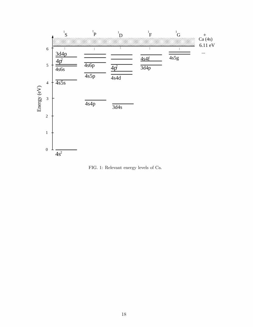
Before solving the TDSE in Eq. (5), however, we must perform several checks regarding

the accuracy of the atomic basis for the singlet states of Ca. The level structure of the

singlet states of Ca is presented in Fig. 1: The first ionization threshold lies at Eion = 6.11

eV relative to the ground state. In Table I we compare our calculated energies with other

theoretical results [7, 9] and the experimental data for the first ionization threshold and the

first few low-lying singlet states for L = S, P,D, and F . The experimental data are taken

from the database of National Institute of Standards and Technology (NIST) [23] and the

energies are taken with respect to the double ionization threshold, Ca2+. From Table I we

notice that our results by the FCHF method provide energy values as accurate as other

theoretical results for the ionization threshold and the first few low-lying states.

The next step is to check the accuracy of the wave function in terms of the OSs. Table II

presents comparisons of the OSs for a single-photon absorption we have calculated with other

theoretical [7, 9] and the experimental data [23, 28–31] for L = S, P,D, and F in both length

and velocity gauges for the following single-photon transitions: 4s2 1Se → 4s(4 − 6)p 1P o

and 3d4p 1P o, 4s4p 1P o → 4s(5 − 7)s 1Se and 4p2 1Se, 4s4p 1P o → 4s(4 − 6)d 1De and

4p2 1De, 4s3d 1De → 4s(4− 6)p 1P o and 3d4p 1P o, and finally 4s3d 1De → 4s(4 − 6)f 1F o

and 3d4p 1F o. Clearly our results on OSs are in good agreement with other theoretical

and experimental data. Relatively large discrepancies appear in the velocity gauge for

the 4s3d 1De → 4s4p 1P o and 4s3d 1De → 3d4p 1F o transitions. This may be due to

the insufficient accuracy of the 3d orbitals. Fortunately the discrepancies appear for the

transitions with very small values of the OSs, and therefore could hardly influence the

outcome of the TDSE calculations we report in this work.

8

After we have checked the accuracy of the constructed atomic basis, we can now proceed

to perform the time-dependent calculations by solving Eq. (9) under various intensities

and photon energies for both LP and CP laser pulses. In the following calculations we

employ 1800 two-electron states for each angular momentum up to L = 9 and carry out the

numerical integration of TDSE [Eq. (9)] using a Runge-Kutta method.

A. Ionization by the second harmonic of a Ti:sapphire laser

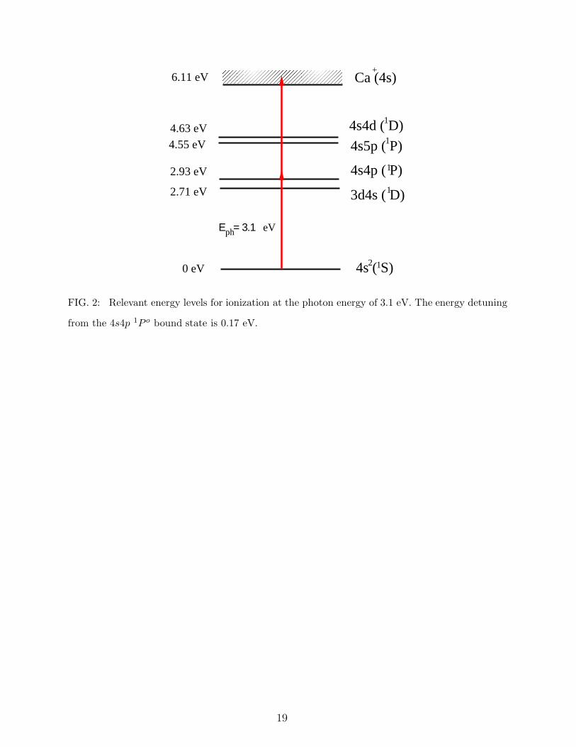
In this subsection we investigate two-photon ionization of Ca by the second harmonic

of the Ti:sapphire laser at the photon energy ω = 3.1 eV, which is schematically shown

in Fig. 2. As already mentioned Ca has a relatively dense level structure and for photons

in the visible range it is quite easy to be near-resonance with some bound states. Indeed,

the detuning from the 4s4p 1P o state is only 0.17 eV, and considering the large value of

the dipole matrix element for the transition 4s2 1Se → 4s4p 1P o (Table II), we expect a

significant enhancement in the ionization signal.

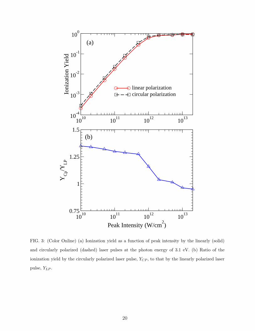
Figure 3(a) shows the ionization yield as a function of peak intensity for LP (solid) and

CP (dashed) laser pulses. The slope of these curves is about 1.85 up to the peak intensity

of I = 5 × 1011 W/cm2, after which the saturation takes place. The calculated slope is a

little bit smaller than the prediction by the lowest order perturbation theory (LOPT) which

gives a slope of 2 for two-photon ionization processes. Figure 3(b) shows the ratio between

the ionization yield by CP and LP laser pulses, YCP/YLP , as a function of peak intensity.

In the low intensity regime (I ≤ 5 × 1011 W/cm2) the ratio slightly decreases with peak

intensity and at peak intensity of 5 × 1011 W/cm2 it is about 1.25, which is smaller than

the ratio predicted by the perturbation theory for the two-photon ionization cross sections

of one-valence-electron atoms, σ(2)CP/σ

(2)LP = 1.4 [32–35].

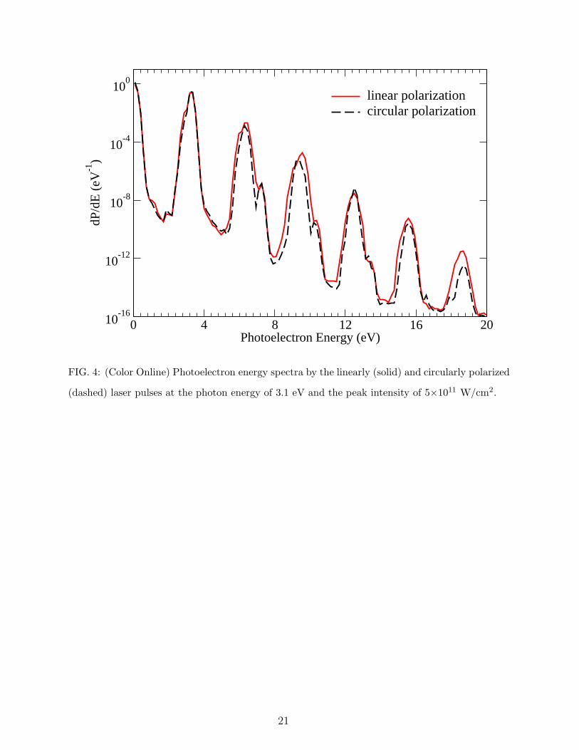
In Fig. 4 we plot the PES for the LP (solid) and CP (dashed) laser pulses at the peak

intensity of I = 5 × 1011 W/cm2. The ATI peaks exhibit some small structures on the left

as well on the right wings which are equidistantly separated by the photon energy. In order

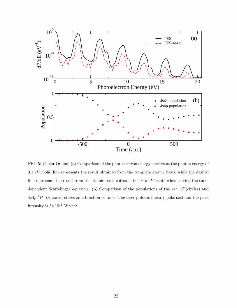
to clarify the importance of the near-resonant bound state 4s4p 1P o we solved the TDSE

with the 4s4p 1P o state artificially removed during the numerical integration. In Fig. 5(a)

we compare the PES (solid) with that calculated without the state 4s4p 1P o (dashed) in the

atomic basis. As a consequence the ionization signal is almost 4 orders of magnitude lower

9

and almost all substructures on the left and right wings of the ATI peaks disappeared when

4s4p 1P o is removed. In order to see the population dynamics of near-resonant 4s4p 1P o,

we plot the population of 4s2 1Se (circles) and 4s4p 1P o (squares) states in Fig. 5(b) as a

function of time. Rabi oscillations take place between them.

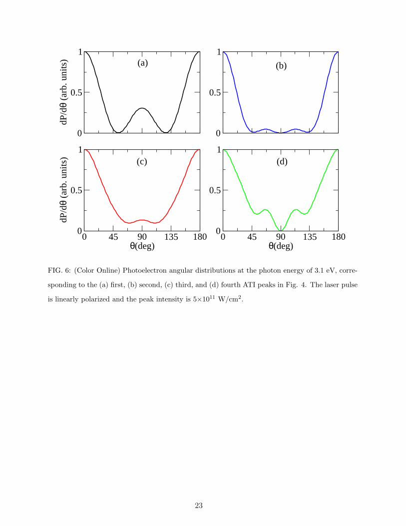
Finally, we show in Figs. 6(a)-6(d) the PADs at the photoelectron energies corresponding

to the first four ATI peaks (see Fig. 4) by the LP pulse at the peak intensity of I = 5×1011

W/cm2. Different ATI peaks exhibit different PADs, since different partial waves make

different contributions with different total phase shifts. This is the reason why the PADs in

Figs. 6(a) and 6(c) and also Figs. 6(b) and 6(d) resemble each other, since the accessible

continua belong to the same parity. We now have a closer look at Fig. 6(a). The PAD

has a typical profile for two-photon ionization from an initial S state with one secondary

maximum at θ = 90◦ and two minima at θ = 54◦ and 126◦, respectively. Similarly the PAD

shown in Fig. 6(b) has a typical profile for three-photon ionization from an initial S state

which exhibits two secondary maxima and three minima. Figures 6(c) and 6(d) present the

PADs at the third and fourth ATI peaks shown in Fig. 4.

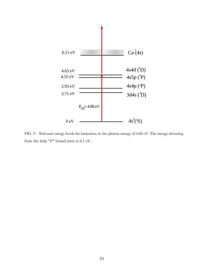
B. Ionization by the third harmonic of a Ti:sapphire laser

In this subsection we study two-photon ionization by the third harmonic of the Ti:sapphire

laser at the photon energy of 4.65 eV, which is schematically shown in Fig. 7. Although

the detuning from the 4s5p 1P o bound state is only 0.1 eV which is even smaller than

the case of the second harmonic in the previous subsection, we do not expect any impor-

tant enhancement in the ionization process because the dipole moment for the transition

4s2 1Se → 4s5p 1P o is much smaller than that for the 4s2 1Se → 4s4p 1P o (see Table II).

Actually the OSs for the 4s2 1Se → 4s5p 1P o transition is anomalously small. This is in

contrast with the more regular decrease of OSs for the 3s2 1Se → 3snp 1P o (n = 3 − 6)

transitions of Mg [16].

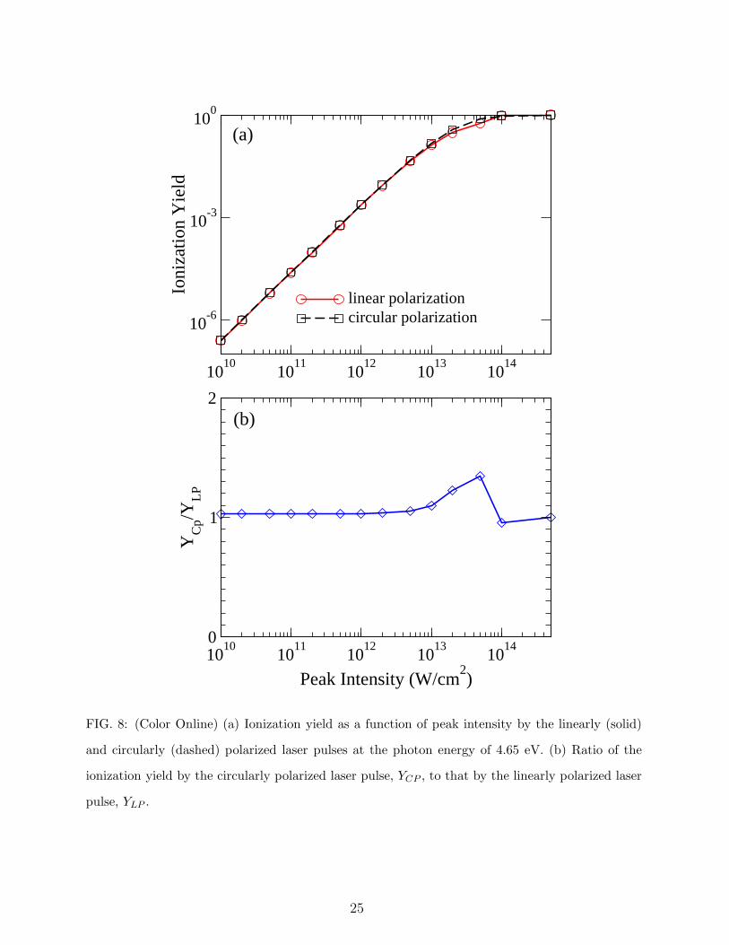
First, we present the ionization yield in Fig. 8(a) as a function of peak intensity for the

LP (solid) and CP (dashed) laser pulses. The curves for the LP and CP laser pulses look

almost the same with a slope of 1.98 at the peak intensities lower than I = 2×1013 W/cm2,

which agrees very well with the LOPT prediction. This implies that the near-resonance

with 4s5p 1P o makes very little contribution to the ionization yield. In Fig. 8(b) the ratio

10

between the ionization yield for CP and LP laser pulses, YCP/YLP , is shown as a function

of peak intensity. We can see that the ionization yield by the LP and CP laser pulses are

almost equal below the saturation intensity.

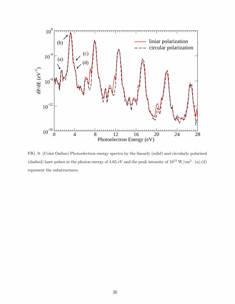
Figure 9 shows the PES by the LP (solid) and CP (dashed) laser pulses at the peak

intensity of I = 1013 W/cm2. Note the large difference of the peak intensities we have

employed for Figs. 4 and 9, which, however, results in the similar amount of the ionization

yields. Interestingly, the PES exhibits more substructures around each ATI peak, labeled

as (a)-(d) in Fig. 9, where substructure (b) is hard to recognize due to the overlap with the

ATI peak. The substructures are equidistantly separated by the photon energy of 4.65 eV

and appear for both LP and CP pulses. These substructures in the PES resemble those we

have seen for Mg at ω = 4.65 eV [4]. The fact that the substructures appear for both LP

and CP pulses implies that the certain bound states accessible in both laser polarization

could be responsible for them. The procedure we have employed to identify the origin of

the substructures is very similar to that we have used for Mg in our previous paper [4]. By

inspection we expect that the bound states 4snp 1P o (n=4,5, and 6) and 3d4p 1P o could

generate such substructures. Since we propagate the TDSE on the atomic basis, we can

easily check this speculation by solving the TDSE by artificially removing the particular

state under suspect, and comparing the PES with the original one obtained by the complete

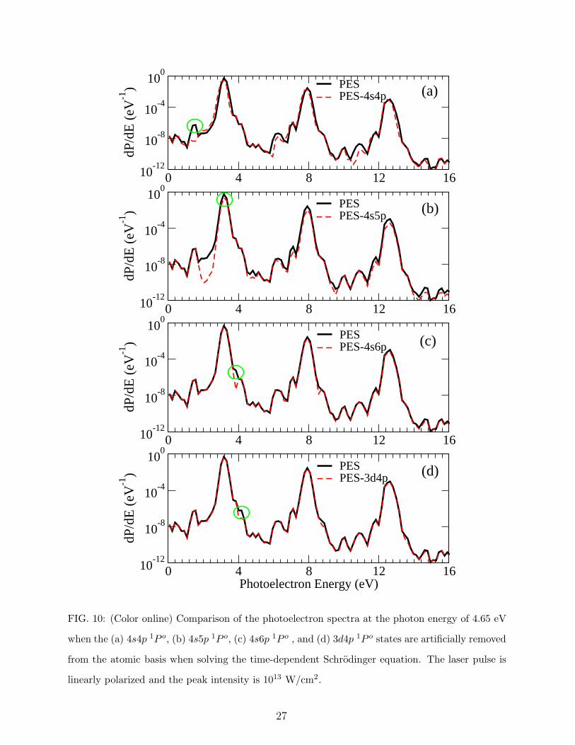
atomic basis. In Figs. 10(a)-10(d) we show the comparisons of the PES calculated under

the same laser parameters with those for Fig. 9. We show the results obtained after the

removal of a particular bound state (dashed lines), namely (a) 4s4p 1P o, (b) 4s5p 1P o, (c)

4s6p 1P o, and (d) 3d4p 1P o upon solving the TDSE, in comparison with the PES for the

complete calculation (solid lines) with the complete atomic basis. When the 4s4p 1P o state

is removed [Fig. 10(a)], the substructures on the left-side of each main peak are reduced

or disappear, as highlighted by the circles. Similarly, by removing the 4s6p 1P o and 3d4p

1P o states in Figs. 10(c) and 10(d), another small spikes labeled as (c) and (d) in Fig. 9

disappear. As for Fig. 10(b) by artificially removing the near-resonant state 4s5p 1P o, the

height of the main ATI peaks is only slightly reduced since the state 4s5p 1P o brings a small

contribution in the ionization process (see Table II). These comparisons indicate that the

physical origin of the substructures labeled as (a)-(d) in Fig. 9 is quite similar to that we

have already found for the singlet as well triplet states of Mg [4, 5]. Briefly, the off-resonant

bound states such as 4s4p 1P o, 4s6p 1P o, and 3d4p 1P o and the near-resonant bound state

11

4s5p 1P o are the origin of the substructures.

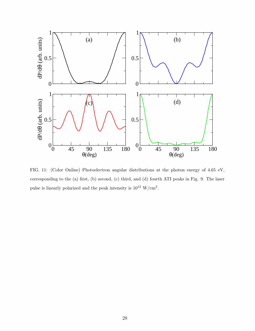
Finally, we show in Figs. 11(a)-11(d) the PADs for the first four ATI peaks in Fig. 9 by

the LP pulse at the peak intensity of I = 1012 W/cm2. The peak intensity is chosen to be

low to avoid any undesired complications at higher intensities. Again, different ATI peaks

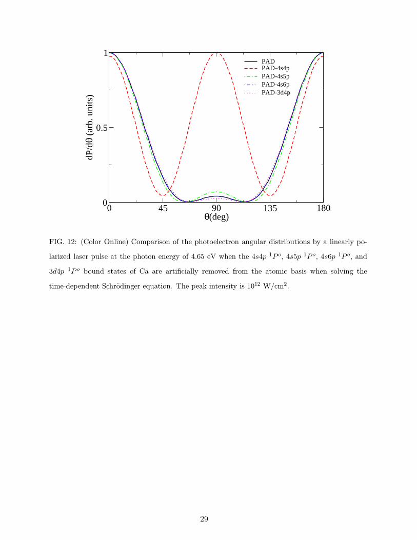
result in the different PADs. In order to examine the influence of the intermediate bound

states with the 1P o symmetry on the PAD we make a comparison of PADs by artificially

removing the 4s4p 1P o (dashed), 4s5p 1P o (dot-dashed), 4s6p 1P o (dot-dot-dashed), and

3d4p 1P o (dot-dotted) states. The results are shown in Fig. 12. It turns out that the PAD

is very sensitive to the removal of the off-resonant 4s4p 1P o state (see Fig. 7), while the

change is very little when other bound states, including the near-resonant 4s5p 1P o state,

are removed.

V. CONCLUSIONS

We have theoretically studied multiphoton ionization of Ca by linearly and circularly

polarized fs laser pulses at the photon energies of 3.1 eV and 4.65 eV in terms of the

ionization yields, photoelectron energy spectra, and photoelectron angular distributions.

At the photon energy of ω = 3.1 eV, the ionization process is strongly enhanced due to

the presence of the near-resonant 4s4p 1P o state which has a large dipole moment from the

ground state, and the ionization yield is about four orders of magnitude larger compared with

a case without a resonance. The photoelectron energy spectrum hardly shows substructures,

because any possible substructures are buried between the strongly enhanced ATI peaks. In

contrast, at the photon energy of ω = 4.65 eV, the photoelectron energy spectrum exhibits

many substructures due to the real excitation of the near-resonant 4s5p 1P o state and some

off-resonant bound states such as 4s4p 1P o, 4s6p 1P o, and 3d4p 1P o, ... etc. Interestingly,

the far off-resonant 4s4p 1P o state still makes a very large contribution to the ionization

processes in this case, which can be most clearly understood in terms of the photoelectron

angular distribution.

12

Acknowledgments

G.B. acknowledges hospitality from the Institute of Advanced Energy, Kyoto University

during her stay. The work by G.B. and T.N. was respectively supported by a research

program from the LAPLAS 3 and CNCSIS contract No. 558/2009 and a Grant-in-Aid for

scientific research from the Ministry of Education and Science of Japan.

13

[1] P. Agostini, F. Fabre, G. Mainfray, G. Petite, and N. K. Rahman, Phys. Rev. Lett. 42, 1127

(1979).

[2] K. Burnett, V. C. Reed, and P. L. Knight, J. Phys. B 26, 561 (1993).

[3] L. F. DiMauro and P. Agostini, Adv. At. Mol. Opt. Phys. 35, 79 (1995).

[4] T. Nakajima and G. Buica, Phys. Rev. A 74, 023411 (2006).

[5] G. Buica and T. Nakajima, Phys. Rev. A 79, 013419 (2009).

[6] C. Froese Fischer and J. E. Hansen, Phys. Rev. A 24, 631 (1981); J. Phys. B 18, 4031 (1985).

[7] J. Mitroy, J. Phys. B 26, 3703 (1993).

[8] M. Aymar, C. H. Greene, and E. Luc-Koenig, Rev. Mod. Phys. 68, 1015 (1996).

[9] J. E. Hansen, C. Laughlin, H. W. van der Hart, and G. Verbockhaven, J. Phys. B 32, 2099

(1999).

[10] C. F. Fischer and G. Tachiev, Phys. Rev. A 68, 012507 (2003).

[11] S. Benec’h and H. Bachau, J. Phys. B 37, 3521 (2004).

[12] L. F. DiMauro, Dalwoo Kim, M. W. Courtney, and M. Anselment, Phys. Rev. A 38, 2338

(1988).

[13] Y.-L. Shao, V. Zafiropoulos, A. P. Georgiadis, and C. Fotakis, Z. Phys. D 21, 299 (1991).

[14] S. Cohen, I. Liontos, A. Bolovinos, A. Lyras, S. Benec’h and H. Bachau, J. Phys. B 39, 2693

(2006).

[15] L. A. A. Nikolopoulos, G. Buica-Zloh, and P. Lambropoulos, Eur. Phys. J. D 26, 245 (2003).

[16] G. Buica and T. Nakajima, J. Quant. Spectrosc. Rad. Transf. 109, 107 (2008).

[17] P. Lambropoulos, P. Maragakis, and J. Zhang, Phys. Rep. 305, 203 (1998).

[18] H. Bachau, E. Cormier, P. Decleva, J. E. Hansen, and F. Martin, Rep. Prog. Phys. 64, 1601

(2001).

[19] T. N. Chang Many-body theory of Atomic Structure and Photoionization, (World Scientific,

Singapore, 1993), p. 213.

[20] X. Tang, T. N. Chang, P. Lambropoulos, S. Fournier, and L. F. DiMauro, Phys. Rev. A 41,

5265 (1990).

[21] T. N. Chang and X. Tang, Phys. Rev. A 46, R2209 (1992).

[22] M. W. J. Bromley and J. Mitroy, Phys. Rev. A 65, 062505-1 (2002).

14

[23] NIST Atomic Spectra Database, http://physics.nist.gov/.

[24] H. J. Werner and W. Meyer, Phys. Rev. A 14, 915 (1976).

[25] R. Moccia and P. Spizzo, J. Phys. B 21, 1133 (1987); 21, 1121 (1988); 21, 1145 (1988); S.

Mengali and R. Moccia, ibid. 29, 1597 (1996).

[26] T. N. Chang and X. Tang, Phys. Rev. A 44, 232 (1991).

[27] A. Burgess, Proc. Phys. Soc. 81, 442 (1963).

[28] W. H. Parkinson, E. M. Reeves, and F. S. Tomkins, J. Phys. B 9, 157 (1976).

[29] G. Smith, J. Phys. B 21, 2827 (1988).

[30] G. Smith and D. St. J. Raggett, J. Phys. B 14, 4015 (1981).

[31] L. P. Lellouch and L. R. Hunter, Phys. Rev. A 36, 3490 (1987).

[32] Y. Gontier and M. Trahin, Phys. Rev. A 7, 2069 (1973).

[33] P. Lambropoulos, Phys. Rev. Lett. 28, 585 (1972).

[34] H. R. Reiss, Phys. Rev. Lett. 29, 1129 (1972).

[35] S. Klarsfeld and A. Maquet, Phys. Rev. Lett. 29, 79 (1972).

15

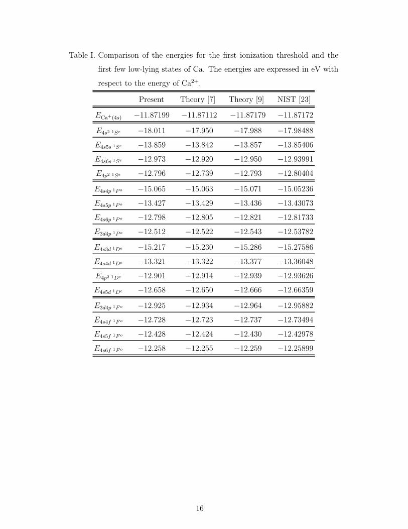
Table I. Comparison of the energies for the first ionization threshold and the

first few low-lying states of Ca. The energies are expressed in eV with

respect to the energy of Ca2+.

Present Theory [7] Theory [9] NIST [23]

ECa+(4s) −11.87199 −11.87112 −11.87179 −11.87172

E4s2 1Se −18.011 −17.950 −17.988 −17.98488

E4s5s 1Se −13.859 −13.842 −13.857 −13.85406

E4s6s 1Se −12.973 −12.920 −12.950 −12.93991

E4p2 1Se −12.796 −12.739 −12.793 −12.80404

E4s4p 1P o −15.065 −15.063 −15.071 −15.05236

E4s5p 1P o −13.427 −13.429 −13.436 −13.43073

E4s6p 1P o −12.798 −12.805 −12.821 −12.81733

E3d4p 1P o −12.512 −12.522 −12.543 −12.53782

E4s3d 1De −15.217 −15.230 −15.286 −15.27586

E4s4d 1De −13.321 −13.322 −13.377 −13.36048

E4p2 1De −12.901 −12.914 −12.939 −12.93626

E4s5d 1De −12.658 −12.650 −12.666 −12.66359

E3d4p 1F o −12.925 −12.934 −12.964 −12.95882

E4s4f 1F o −12.728 −12.723 −12.737 −12.73494

E4s5f 1F o −12.428 −12.424 −12.430 −12.42978

E4s6f 1F o −12.258 −12.255 −12.259 −12.25899

16

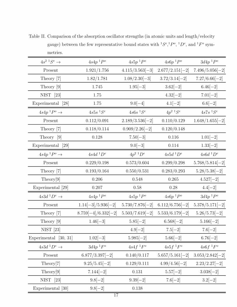
Table II. Comparison of the absorption oscillator strengths (in atomic units and length/velocity

gauge) between the few representative bound states with 1Se,1P o, 1De, and 1F o sym-

metries.

4s2 1Se → 4s4p 1P o 4s5p 1P o 4s6p 1P o 3d4p 1P o

Present 1.921/1.756 4.115/3.563[−3] 2.677/2.151[−2] 7.496/5.056[−2]

Theory [7] 1.82/1.781 1.08/2.30[−3] 3.72/3.14[−2] 7.27/6.66[−2]

Theory [9] 1.745 1.95[−3] 3.62[−2] 6.46[−2]

NIST [23] 1.75 4.32[−2] 7.01[−2]

Experimental [28] 1.75 9.0[−4] 4.1[−2] 6.6[−2]

4s4p 1P o → 4s5s 1Se 4s6s 1Se 4p2 1Se 4s7s 1Se

Present 0.112/0.091 2.189/3.536[−2] 0.110/0.129 1.648/1.655[−2]

Theory [7] 0.118/0.114 0.909/2.26[−2] 0.120/0.148

Theory [9] 0.128 7.50[−3] 0.116 1.01[−2]

Experimental [29] 9.0[−3] 0.114 1.33[−2]

4s4p 1P o → 4s4d 1De 4p2 1De 4s5d 1De 4s6d 1De

Present 0.229/0.198 0.573/0.604 0.299/0.298 5.768/5.814[−2]

Theory [7] 0.193/0.164 0.550/0.531 0.283/0.293 5.28/5.38[−2]

Theory[9] 0.206 0.548 0.265 4.527[−2]

Experimental [29] 0.207 0.58 0.28 4.4[−2]

4s3d 1De → 4s4p 1P o 4s5p 1P o 4s6p 1P o 3d4p 1P o

Present 1.14[−3]/5.936[−2] 5.730/7.876[−2] 6.112/6.756[−2] 5.378/5.171[−2]

Theory [7] 8.759[−4]/6.332[−2] 5.503/7.619[−2] 5.533/6.179[−2] 5.26/5.73[−2]

Theory [9] 1.46[−3] 5.85[−2] 6.568[−2] 5.166[−2]

NIST [23] 4.9[−2] 7.5[−2] 7.6[−2]

Experimental [30, 31] 1.02[−3] 5.985[−2] 5.66[−2] 6.76[−2]

4s3d 1De → 3d4p 1F o 4s4f 1F o 4s5f 1F o 4s6f 1F o

Present 6.877/3.397[−2] 0.140/0.117 5.657/5.161[−2] 3.053/2.842[−2]

Theory[7] 9.25/5.45[−2] 0.129/0.111 4.99/4.56[−2] 2.23/2.27[−2]

Theory[9] 7.144[−2] 0.131 5.57[−2] 3.038[−2]

NIST [23] 9.8[−2] 9.39[−2] 7.6[−2] 3.2[−2]

Experimental [30] 9.8[−2] 0.138

17

1+

1 111

24p

D

... ...

4s4p

4s6p 4s4f

24p

...

4s5p 4s6s

4s5s

3d4s

4s4d

3d4p

4s5g

P

...

G

...

FS

24s

3d4p

��������������������������������������������������������������������������������������������������������������������������������������������������������������������������������������������

��������������������������������������������������������������������������������������������������������������������������������������������������������������������������������������������

Ene

rgy

(eV

)

2

1

3

6

5

4

0

...

Ca (4s)6.11 eV

FIG. 1: Relevant energy levels of Ca.

18

124s ( S)

13d4s ( D)

14s4p ( P)

Ca (4s)+

14s4d ( D)

eVΕ = 3.1 ph

14s5p ( P)

���������������������������������������������������

���������������������������������������������������

0 eV

2.71 eV

2.93 eV

4.55 eV4.63 eV

6.11 eV

FIG. 2: Relevant energy levels for ionization at the photon energy of 3.1 eV. The energy detuning

from the 4s4p 1P o bound state is 0.17 eV.

19

1010

1011

1012

101310

-4

10-3

10-2

10-1

100

Ioni

zatio

n Y

ield

linear polarizationcircular polarization

1010

1011

1012

1013

Peak Intensity (W/cm2)

0.75

1

1.25

1.5

YC

p/YL

P

(a)

(b)

FIG. 3: (Color Online) (a) Ionization yield as a function of peak intensity by the linearly (solid)

and circularly polarized (dashed) laser pulses at the photon energy of 3.1 eV. (b) Ratio of the

ionization yield by the circularly polarized laser pulse, YCP , to that by the linearly polarized laser

pulse, YLP .

20

0 4 8 12 16 20Photoelectron Energy (eV)

10-16

10-12

10-8

10-4

100

dP/d

E (

eV-1

)linear polarizationcircular polarization

FIG. 4: (Color Online) Photoelectron energy spectra by the linearly (solid) and circularly polarized

(dashed) laser pulses at the photon energy of 3.1 eV and the peak intensity of 5×1011 W/cm2.

21

-500 0 500Time (a.u.)

0

0.5

1

Popu

latio

n

4s4s population 4s4p population

0 5 10 15 20Photoelectron Energy (eV)

10-16

10-8

100

dP/d

E (

eV-1

) PESPES-4s4p

(a)

(b)

FIG. 5: (Color Online) (a) Comparison of the photoelectron energy spectra at the photon energy of

3.1 eV. Solid line represents the result obtained from the complete atomic basis, while the dashed

line represents the result from the atomic basis without the 4s4p 1P o state when solving the time-

dependent Schrodinger equation. (b) Comparison of the populations of the 4s2 1Se(circles) and

4s4p 1P o (squares) states as a function of time. The laser pulse is linearly polarized and the peak

intensity is 5×1011 W/cm2.

22

0

0.5

1dP

/dθ

(arb

. uni

ts)

0

0.5

1

0 45 90 135 180θ(deg)

0

0.5

1

dP/d

θ (a

rb. u

nits

)

0 45 90 135 180θ(deg)

0

0.5

1

(a) (b)

(d)(c)

FIG. 6: (Color Online) Photoelectron angular distributions at the photon energy of 3.1 eV, corre-

sponding to the (a) first, (b) second, (c) third, and (d) fourth ATI peaks in Fig. 4. The laser pulse

is linearly polarized and the peak intensity is 5×1011 W/cm2.

23

124s ( S)

13d4s ( D)

14s4p ( P)

eVΕ = 4.65 ph

Ca (4s)+

14s4d ( D)14s5p ( P)

���������������������������������������������������

���������������������������������������������������

0 eV

2.71 eV

2.93 eV

4.55 eV4.63 eV

6.11 eV

FIG. 7: Relevant energy levels for ionization at the photon energy of 4.65 eV. The energy detuning

from the 4s5p 1P o bound state is 0.1 eV.

24

1010

1011

1012

1013

1014

10-6

10-3

100

Ioni

zatio

n Y

ield

linear polarizationcircular polarization

1010

1011

1012

1013

1014

Peak Intensity (W/cm2)

0

1

2

YC

p/YL

P

(a)

(b)

FIG. 8: (Color Online) (a) Ionization yield as a function of peak intensity by the linearly (solid)

and circularly (dashed) polarized laser pulses at the photon energy of 4.65 eV. (b) Ratio of the

ionization yield by the circularly polarized laser pulse, YCP , to that by the linearly polarized laser

pulse, YLP .

25

0 4 8 12 16 20 24 28Photoelectron Energy (eV)

10-16

10-12

10-8

10-4

100

dP/d

E (

eV-1

)liniar polarizationcircular polarization

(b)

(a)(c)

(d)

FIG. 9: (Color Online) Photoelectron energy spectra by the linearly (solid) and circularly polarized

(dashed) laser pulses at the photon energy of 4.65 eV and the peak intensity of 1013 W/cm2. (a)-(d)

represent the substructures.

26

0 4 8 12 1610-12

10-8

10-4

100

dP/d

E (

eV-1

) PESPES-4s4p

0 4 8 12 1610-12

10-8

10-4

100

dP/d

E (

eV-1

)

PESPES-4s5p

0 4 8 12 1610-12

10-8

10-4

100

dP/d

E (

eV-1

)

PESPES-4s6p

0 4 8 12 16Photoelectron Energy (eV)

10-12

10-8

10-4

100

dP/d

E (

eV-1

)

PES PES-3d4p

(a)

(b)

(c)

(d)

FIG. 10: (Color online) Comparison of the photoelectron spectra at the photon energy of 4.65 eV

when the (a) 4s4p 1P o, (b) 4s5p 1P o, (c) 4s6p 1P o , and (d) 3d4p 1P o states are artificially removed

from the atomic basis when solving the time-dependent Schrodinger equation. The laser pulse is

linearly polarized and the peak intensity is 1013 W/cm2.

27

0

0.5

1dP

/dθ

(arb

. uni

ts)

0

0.5

1

0 45 90 135 180θ(deg)

0

0.5

1

dP/d

θ (a

rb. u

nits

)

0 45 90 135 180θ(deg)

0

0.5

1

(a)

(c) (d)

(b)

FIG. 11: (Color Online) Photoelectron angular distributions at the photon energy of 4.65 eV,

corresponding to the (a) first, (b) second, (c) third, and (d) fourth ATI peaks in Fig. 9. The laser

pulse is linearly polarized and the peak intensity is 1012 W/cm2.

28

0 45 90 135 180θ(deg)

0

0.5

1

dP/d

θ (a

rb. u

nits

)

PADPAD-4s4pPAD-4s5pPAD-4s6pPAD-3d4p

FIG. 12: (Color Online) Comparison of the photoelectron angular distributions by a linearly po-

larized laser pulse at the photon energy of 4.65 eV when the 4s4p 1P o, 4s5p 1P o, 4s6p 1P o, and

3d4p 1P o bound states of Ca are artificially removed from the atomic basis when solving the

time-dependent Schrodinger equation. The peak intensity is 1012 W/cm2.

29