International Journal of Heat and Mass Transfer 55 (2012) 6994–7004

Contents lists available at SciVerse ScienceDirect

International Journal of Heat and Mass Transfer

journal homepage: www.elsevier .com/locate / i jhmt

Instability of pressure driven viscous fluid streams in a microchannelunder a normal electric field

Haiwang Li, Teck Neng Wong ⇑, Nam-Trung NguyenSchool of Mechanical and Aerospace Engineering, Nanyang Technological University, 50 Nanyang Avenue, Singapore 639798, Singapore

a r t i c l e i n f o a b s t r a c t

Article history:Received 18 January 2012Received in revised form 4 July 2012Accepted 5 July 2012Available online 31 July 2012

Keywords:ElectrohydrodynamicConstant flow rateLinear instabilityMicrochannel

0017-9310/$ - see front matter � 2012 Elsevier Ltd. Ahttp://dx.doi.org/10.1016/j.ijheatmasstransfer.2012.07

⇑ Corresponding author.E-mail address: mtnwong@ntu.edu.sg (T.N. Wong)

This paper investigates analytically and experimentally electrohydrodynamic instability of the interfacebetween two viscous fluids with different electrical properties under constant flow rates in a microchan-nel. In the three-dimensional analytical model, the two-layer system is subjected to an electric field nor-mal to the interface between the two fluids. There is no assumption on the magnitude of the ratio of fluidto electric time scales, and thus the linear Poisson–Boltzmann equation are solved using separation ofvariable method for densities of bulk charge and surface charge. The electric field and fluid dynamicsare coupled only at the interface through the tangential and normal interfacial stress balance equations.In the experiments, two immiscible fluids, aqueous NaHCO3 (the high electrical mobility fluid) and sili-cone oil (polydimethylsiloxane, the low electrical mobility fluid) are pumped into a microchannel madein polymethyl methacrylate) (PMMA) substrate. The normal electric field is added using a high voltagepower supply. The results showed that the external electric field and increasing width of microchanneldestabilize the interface between the immiscible fluids. At the same time, the viscosity of the high elec-trical mobility fluid and flow rates of fluids has a stabilizing effect. The experimental results and theanalytical results show a reasonable agreement.

� 2012 Elsevier Ltd. All rights reserved.

1. Introduction

In microfluidic devices, interfacial instability can produce a vari-ety of flow patterns or even develop into turbulence. In a micro-channel, viscous force dominates and mixing by inertia driventurbulence is impossible. On the one hand, the possibility of usinginstability to achieve efficient mixing using different methodswas explored by various groups [1–3]. On the other hand, stableflow is crucial for pumping immiscible liquids [4,5]. The identifica-tion of parameters for interfacial instability is necessary for control-ling the flow pattern. In many conditions, electro-osmotic flow isthe primary method of fluid handing [6]. Electrohydrodynamics isregarded as a branch of fluid mechanics concerned with the effectof electric forces. The field is also considered as a part of electrody-namics involving the interaction between moving media and elec-tric fields [7].

The electrohydrodynamic instability theory was pioneered byTaylor and Melcher using the leaky dielectric model [7]. In general,there are two modeling approaches in the presence of interfaceinstability.

ll rights reserved..012

.

The first approach is the bulk coupled model that assumes aconductivity gradient in a thin diffusion layer between the twofluids, resulting in an electrical body force on the fluid. The interac-tion between the conductivity gradient and high electric field playsa critical role in the generation of interface instability. A number ofresearchers studied the effect of conductivity gradient and highelectric field [8–12]. Comparing with the work of Oddy et al. [1],Chen and Santiago [8] provided a more systematic investigationto establish the critical importance of conductivity gradient andhigh electric field strength for inducing the instability. The resultsshowed that the conductivity gradient and their associated bulkcharge accumulation are crucial for instability. Lin et al. [9] studiedtemporal instability in a T-junction merging two fluid streams ofdifferent conductivities via linear stability analysis, experiments,and numerical simulations. All the methods show that there arethresholds where the electric body force is too great for diffusionto quench. In this flow, the electric field was normal to the conduc-tivity gradient. Chen et al. [10] used experiments and linear stabil-ity analysis to study convective instability occurring in anelectroosmotic flow [9]. Using the method of numerical simula-tions, Storey [11] showed the generation of turbulence with a rel-atively low Reynolds number, and evaluated the effects of differentassumptions in boundary conditions of nonlinear behavior andmixing. Kang et al. [12] studied the initial growth of electrohydro-dynamic instability via numerical simulation. The results showed

H. Li et al. / International Journal of Heat and Mass Transfer 55 (2012) 6994–7004 6995

that the molecular diffusion has a dual role in the onset and thedevelopment of instability and the system is unstable to high elec-tric fields even without any external disturbances.

The second approach is the surface coupled model that consid-ers a jump in electrical conductivity at the interface of the twofluids. In this method, the bulk electrical force is vanished. The dis-continuity of the electrical properties of the fluids across the inter-face affects the force balance at the fluid–fluid interface, whichmay either stabilize or destabilize the interface. Mohamed et al.[13] analyzed the stability of the Couette-Poiseuille flow. Theresults showed that the velocity stratification affects the stabilityof the fluids. The normal electric field is greatly reduced by the in-crease of the thickness of the non-conducting fluid layer. Abdellaand Rasmussen [14] analyzed Couette flow in an unbounded do-main subjected to a normal electric field. Two special cases, theelectrohydrodynamic free-charge case and the electrohydrody-namic polarization charge configuration, were analyzed using Ariyfunctions and Ariy integrals [14]. Thaokar and Kumaran [15] ana-lyzed the stability of the interface between two dielectric fluidsconfined between parallel plates subjected to a normal electricfield in the limit of zero Reynolds number. The results indicatedthat the interface becomes unstable when the electric field exceedsa critical value, and the critical value are influenced by the ratio ofdielectric constant, ratio of viscosities, ratio of thickness, and sur-face tension. The results also showed that for a small wave number(k), the critical potential increases proportional to k. For a largewave number, the critical potential increases proportional to thesquare root of k. Ozen et al. [16] analyzed the linear stability ofthe interface between two immiscible fluids and found the effectsof electric fields and mechanical properties to the instability of theinterface. Moatimid and Obied Allah [17] investigated the linearsurface wave instability between two finite fluid layers. The fluidlayers have different electric properties and are subjected to anelectric field normal to their interface. The surface tension showedto have a stabilizing influence, while the streaming velocity wasstrictly destabilizing.

Using the surface coupled model, Goranovic [18] analyticallyinvestigated the instability of two immiscible inviscid fluids inmicrochannels under static state; the effect of interfacial freecharge was ignored. The aim of the present paper is to study theeffect of normal electric fields on two immiscible viscid fluids un-der the combined effect of hydrodynamic and electroosmosis inmicrochannels. The effects of viscosity and surface charge are in-cluded in the analysis. In the analytical model, electric field andfluid dynamics are coupled at the interface through the tangentialand normal interfacial stress balance equations. The instability ofthe interface between conducting fluid and non-conducting fluidis both analytically and experimentally investigated.

2. The physical and mathematical model

2.1. Methodology and approach

The usual procedure in linear stability analysis can follow six ba-sic steps. In the first step, general governing equations and generalboundary conditions are introduced. The governing equations con-trol the initial and stationary flow conditions in the velocity field V0.The governing equations include the continuity equation, themomentum equations, the Maxwell equations and the Poisson–Boltzmann equation.

In the second step, the perturbation of v0 is introduced andsuperposed to the stationary velocity V0. The velocity field changesinto v = v0 + v0. Substituting the equation into governing equationsand boundary conditions, the equations governing the perturba-tion are obtained.

In the third step, the equations governing the perturbation arelinearized, the terms with quadratic and higher terms in v0 areneglected.

In the forth step, the perturbation quantities v0 are furtherexpressed in terms of normal modes. A spatially and temporallyperiodic perturbation can be assumed in the form of v0kðr; tÞ ¼vkðzÞ expð�ixktÞ expðiðk � rÞÞ.

In the fifth step, the perturbation v0kðr; tÞ ¼ vkðzÞ expð�ixktÞexpðiðk � rÞÞ is substituted into the governing equations, the tempo-ral stability can be solved. The complex solution for xk can bedescribed as xk = Real (xk) + iIm(xk).

In the sixth step, the freely evolving waves are spatially periodicdisturbances of infinite spatial extent which travel with a phasevelocity, cr �xr/k and grow or decrease in amplitude with a tem-poral growth rate, Imxk. The system is considered to be linearlyunstable to infinitesimal disturbances for Imxk > 0. The stabilityregimes can be distinguished as instable (Imxk > 0), neutral(Imxk = 0) and stable (Imxk < 0).

2.2. General equations of motion

Fig. 1(a) shows the stability of the interface between twoimmiscible fluids under the combined effect of hydrodynamicand electroosmosis. Fluid 1 is conducting with high electroosmoticmobility and fluid 2 is non-conducting with low electroosmoticmobility. The flows are induced by the pressure source and theelectric field. The two fluids have different properties. The appliedelectric field is normal to the unperturbed interface. Fig. 1(c) showsthe cross sectional view of the two fluids in the rectangular micro-channel, h1 and h2 are denoted as the fraction of fluid 1 and fluid 2,respectively.

The following notation will be used: superscripts (1) and (2)denote quantities pertaining to fluid 1 and fluid 2. The prime sym-bol (0) indicates a perturbed variable; the subscript 0 denotes theunperturbed variables; other subscripts are used for vectorcomponent.

The momentum equation for an isotropic incompressibleNewtonian liquid is given by

qðjÞDvðjÞ

Dt¼ �rPðjÞ þ lðjÞr2vðjÞ þ FðjÞe ðj ¼ 1;2Þ ð1Þ

where q is the density, P the pressure, l the dynamical viscosity, vthe velocity, Fe the electric body force. In microsystems, the effect ofgravity can be ignored [18]. In the case of a homogeneous dielectric,the permittivity is constant, and the electric force Fe reduces to [18]

Fe ¼ qeE ð2Þ

where qe is the density of electric charge, E is the electric field. Thecontinuity equation for incompressible liquids is

r � vðjÞ ¼ 0 ðj ¼ 1;2Þ ð3Þ

Assuming that the electric charge density is not affected by theexternal electric field due to thin EDLs and the small fluid velocity,the charge convection can be ignored and the electric field equa-tion and the fluid flow equation are decoupled [19,20]. Accordingthe previous work [5,21,22], the governing equations for the freecharge can be described as

r2w ¼ 2z0en0

esinh

ziewkbT

� �ð4Þ

and

qe ¼ �2z0en0 sinhðziew=kbTÞ ð5Þ

where w is the electric potential, z0 is the valence of the ions, e is ele-mentary charge, n0 is the reference value of the ion concentration, e

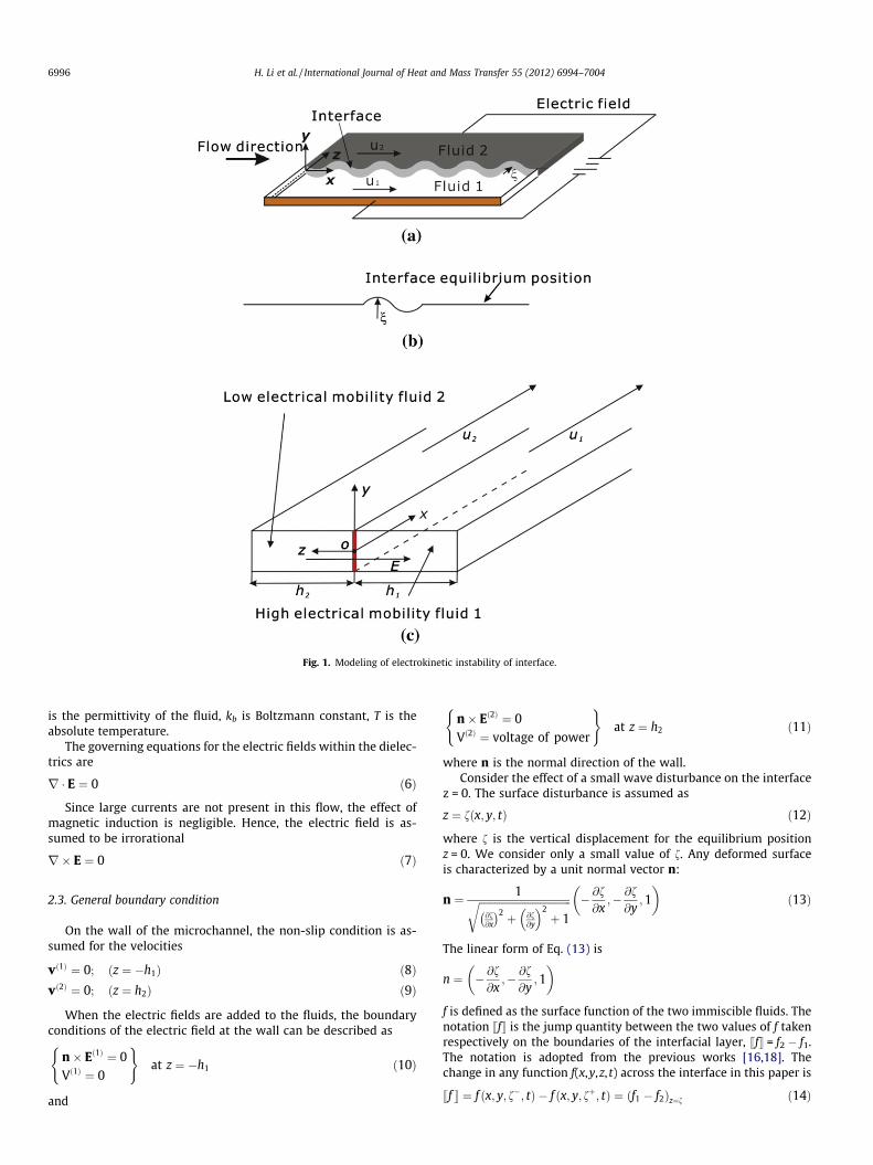
Fig. 1. Modeling of electrokinetic instability of interface.

6996 H. Li et al. / International Journal of Heat and Mass Transfer 55 (2012) 6994–7004

is the permittivity of the fluid, kb is Boltzmann constant, T is theabsolute temperature.

The governing equations for the electric fields within the dielec-trics are

r � E ¼ 0 ð6Þ

Since large currents are not present in this flow, the effect ofmagnetic induction is negligible. Hence, the electric field is as-sumed to be irrorational

r� E ¼ 0 ð7Þ

2.3. General boundary condition

On the wall of the microchannel, the non-slip condition is as-sumed for the velocities

vð1Þ ¼ 0; ðz ¼ �h1Þ ð8Þvð2Þ ¼ 0; ðz ¼ h2Þ ð9Þ

When the electric fields are added to the fluids, the boundaryconditions of the electric field at the wall can be described as

n� Eð1Þ ¼ 0Vð1Þ ¼ 0

( )at z ¼ �h1 ð10Þ

and

n� Eð2Þ ¼ 0Vð2Þ ¼ voltage of power

( )at z ¼ h2 ð11Þ

where n is the normal direction of the wall.Consider the effect of a small wave disturbance on the interface

z = 0. The surface disturbance is assumed as

z ¼ fðx; y; tÞ ð12Þ

where f is the vertical displacement for the equilibrium positionz = 0. We consider only a small value of f. Any deformed surfaceis characterized by a unit normal vector n:

n ¼ 1ffiffiffiffiffiffiffiffiffiffiffiffiffiffiffiffiffiffiffiffiffiffiffiffiffiffiffiffiffiffiffiffiffiffiffiffi@f@x

� �2 þ @f@y

� �2þ 1

r � @f@x;� @f

@y;1

� �ð13Þ

The linear form of Eq. (13) is

n ¼ � @f@x;� @f

@y;1

� �f is defined as the surface function of the two immiscible fluids. Thenotation sft is the jump quantity between the two values of f takenrespectively on the boundaries of the interfacial layer, sft = f2 � f1.The notation is adopted from the previous works [16,18]. Thechange in any function f(x,y,z, t) across the interface in this paper is

sf t ¼ f ðx; y; f�; tÞ � f ðx; y; fþ; tÞ ¼ ðf1 � f2Þz¼f ð14Þ

H. Li et al. / International Journal of Heat and Mass Transfer 55 (2012) 6994–7004 6997

where the superscripts of – and + means the side of interface facingfluid 1 an fluid 2 respectively. At the interface z = f, the continuity ofvelocities are

sut ¼ svt ¼ swt ¼ 0 ð15Þ

wð1Þ ¼ wð2Þ ¼ dfdt

ð16Þ

where u, v, w are the velocities along x, y, z directions respectively.The continuity of normal electrical fields at the interface can be

described as

n � seEt ¼ 0 ð17Þn� sEt ¼ 0 ð18Þ

The stress balance at any part on the interface can be describedusing the following equation

s� ptni þ ssik þ TMik tnk þ qs � Ei ¼ rr2

s fni ð19Þ

where p is the pressure, sik is the viscous stress, TM is the Maxwellstress tensor, qs is the surface charge which can be calculated in theprevious works [5,22], r is the surface tension, r2

s f describes thesurface curvature for small deformations, the subscripts of i and kmean the vector component i = x,y,z and k = x,y,z.

2.4. Perturbation equations

The analysis involves the assumption that the perturbations tothe base state are infinitesimally small. To carry out a linear stabil-ity analysis, all high-order terms in the perturbation quantities areneglected. The expanding solutions are

v ¼ v0 þ v0 þ � � � ð20Þp ¼ p0 þ p0 þ � � � ð21Þ

2.4.1. The base state solutionIn the base state, the velocity field and the electric field can be

described by the unperturbed equations. Under unperturbed con-dition, Eqs. (20) and (21) transform into

v ¼ v0 ð22Þp ¼ p0 ð23Þ

The governing equations of Eqs. (1) and (3) can be transformed intothe base state equations:

@ðqv0Þ@�t

¼ �rp0 þ lr2v0 ð24Þ

r � v0 ¼ 0 ð25Þ

The details of velocity profile and pressure gradient have beendescribed previously [5].

The vector n normal to the unperturbed interface is given by

n0 ¼ ð0;0;1Þ ð26Þ

The stress balance at the interface can be described as followingequations [18]:

sP0tnx ¼ sP0tny ¼ 0 ð27Þ

sP0tnz ¼ sPtþ 12� seE2

z0tþ qs � Ez0 ð28Þ

where the subscripts of nx, ny and nz means three components ofnormal vector in x, y and z directions respectively.

2.4.2. Linearization of the perturbed equationsUnder perturbed condition, Eqs. (1) and (3) transform into

@ðqðv0 þ v0ÞÞ@t

¼ �rðp0 þ p0Þ þ lr2ðv0 þ v0Þ ð29Þ

r � ðv0 þ v0Þ ¼ 0 ð30Þ

In this section, the changes in the density, viscosity, and chargedensity are not considered since they are assumed to be constantin each region. When subtracting the base state of Eqs. (24) and(25) from Eqs. (29) and (30), the equations reduce to

q@v0

@t¼ �rp0 þ 1

Relr2v0 ð31Þ

r � u0 ¼ 0 ð32Þ

Combing Eqs. (31) and (32) leads to

r2p0 ¼ 0 ð33Þ

For a constant charge density, the electric field can be described as

r2E0x ¼ 0 ð34Þ

As the electric field is irrorational, the governing equation for E0 is

r� E0 ¼ 0 ð35Þ

2.4.3. Linearization of the perturbed boundary conditions of rigidboundaries

The boundary of the wall under perturbed conditions can be lin-earized as following

wð1Þ0 ¼ uð1Þ0 ¼ v ð1Þ

0 ¼ 0 at z ¼ ��h1 ð36Þwð2Þ0 ¼ uð2Þ

0 ¼ v ð2Þ0 ¼ 0 at z ¼ �h2 ð37Þ

n0 � Eð1Þ0¼ 0 at z ¼ ��h1 ð38Þ

n0 � Eð2Þ0¼ 0 at z ¼ �h2 ð39Þ

2.4.4. Linearization of the perturbed boundary conditions of theinterface

Since f is assumed to be small, the first order approximation

E0ið0þ fÞ ¼ E0ið0Þ þ@E0ið0Þ@z

� fþ � � � � E0ið0Þ ð40Þ

is valid if both E0i and f remains small. In Eq. (40), E0ið0Þ is the pertur-bation of electric field at z = 0 and E0ið0þ fÞ is the perturbation ofelectric field at z = f. The normal vector is now

n ¼ n0 þ n0 ð41Þ

where n0 is

n0 ¼ � @f@x;� @f

@y;0

� �ð42Þ

The boundary conditions for perturbation at z = f are

su0t ¼ sv 0t ¼ sw0t ¼ 0 ð43Þ

w0ð0Þ ¼ dfdt

ð44Þ

The electric fields is described as

E ¼ E0x; E0y; Ez0 þ E0z

� �: ð45Þ

The boundary condition of Eqs. (17) and (18) at the interface is

sE0x þ Ez0@f@x

t ¼ 0 ð46Þ

seE0zt ¼ 0: ð47Þ

6998 H. Li et al. / International Journal of Heat and Mass Transfer 55 (2012) 6994–7004

2.4.5. Linearized stressesIn a microsystem, the effect of gravity is ignored. Substituting

Eq. (21) into Eq. (19), the stress conditions of the interface can bedescribed as

�sp0tni � sPtni þ ssik þ TMik tnk þ qs � Ei ¼ rr2

s fni ð48Þ

Eq. (48) can be transformed into following equations in x, y, zdirections

seE2z0tþ sPt

� �� @f@xþ l @u0

@zþ @w0

@x

� � þ qs � E0x þ seEz0E0xt ¼ 0 ð49Þ

seE2z0tþ sPt

� �� @f@yþ l @v 0

@zþ @w0

@y

� � þ qs � E

0y þ seEz0E0yt ¼ 0 ð50Þ

� sp0tþ 2l @w0

@zþ seEz0E0ztþ qs � E

0z ¼ rr2

s f ð51Þ

2.4.6. Expansion in normal modesThe perturbation can be expanded into the normal model using

the following equations

f ¼ f exp½iðkxxþ kyyÞ þ nt� ð52Þv0 ¼ vðzÞ exp½iðkxxþ kyyÞ þ nt� ð53Þp0 ¼ pðzÞ exp½iðkxxþ kyyÞ þ nt� ð54ÞE0i ¼ bEiðzÞ exp½iðkxxþ kyyÞ þ nt� ð55Þ

where n = �ix, x is the complex phase velocity of the disturbance,k2 ¼ k2

x þ k2y ; k is the magnitude of the total wave number, i is the

standard imaginary unit. Using Eqs. (52)–(55), the stress balanceat the interface (Eq. (49)) is transformed as

seE2z0tþ sPt

� �k2 fþ l d

dz

2

þ k2

!w

" #" #þ qs �

dEz

dz

" #" #þ eEz0

dEz

dz

" #" #¼ 0 ð56Þ

2.4.7. Solutions and linearized boundary conditionsAccording the boundary conditions and the properties of the

perturbation, the boundary conditions for velocity (Eqs. (8) and(9)) and electric field (Eqs. (10) and (11)) can be described as follow

wð1Þ ¼ A sinh kðzþ �h1Þ ð57Þwð2Þ ¼ B sinh kðz� �h2Þ ð58ÞbEð1Þx ¼ C1 expðkzÞ þ C2 expð�kzÞ ð59ÞbEð2Þx ¼ D1 expðkzÞ þ D2 expð�kzÞ ð60Þ

bEy ¼ky

kxEx ð61Þ

bEz ¼1

ikx

@Ex

@zð62Þ

Substituting Eqs. (57)–(62) into the boundary conditions of Eqs.(36)–(39), the boundary conditions transform into

wð1Þð��h1Þ ¼ 0 ð63Þwð2Þð�h2Þ ¼ 0 ð64ÞbEð1Þx ð��h1Þ ¼ bEð1Þy ð��h1Þ ¼ bEð1Þz ð��h1Þ ¼ 0 ð65ÞbEð2Þx ð�h2Þ ¼ bEð2Þy ð�h2Þ ¼ Eð2Þz ð�h2Þ ¼ 0 ð66Þ

At the interface, the continuity of velocities of perturbation for bothfluids has the same values; this condition transforms into

swð0Þt ¼ dwð0Þdz

¼ 0 ð67Þ

Combining Eqs. 44, 52 and 57, we can obtain that

f ¼ wð1Þð0Þðnþ u � ikxÞ

¼ wð1Þð0Þm

ð68Þ

where

m ¼ nþ u � ikx ð69ÞEqs. (46)–(48) describing the stress balance at the interface is trans-formed into the following form:

dðbEzð0ÞÞdz

þ k2Ez0 �wð0Þ

m

" #" #¼ 0 ð70Þ

sebEzð0Þt ¼ 0 ð71Þ

�qnþ ld2

dz� 3k2

!" #dwð0Þ

dz

" #" #� k2

seEz0bEzð0Þtþ qs � sbEzð0Þtþ rk2 wð1Þð0Þ

m

� �¼ 0 ð72Þ

seE2z0tþ sPtþ qs � sEz0t

� �k2 wð1Þð0Þ

mþ l d2

dzþ k2

!wð0Þ

" #" #

þ qs �dbEzð0Þ

dz

" #" #þ eEz0

dbEzð0Þdz

" #" #¼ 0 ð73Þ

2.5. The principle of exchange of stabilities

In Eq. (52), if n < 0, the disturbances decay exponentially to zeroas time lapses. The disturbance cannot induce the instability of theinterface and the two-fluid electroosmotic flow is stable. If n > 0,the disturbances advance exponentially to a large value as timelapses. The disturbance can be enlarged to induce the instabilityof the interface, and the two-fluid electroosmotic flow is unstable.According the boundary conditions, Eqs. (57)–(60) reduce to

wð1Þ ¼ A sinh kðzþ �h1Þ ð74Þwð2Þ ¼ B sinh kðz� �h2Þ ð75ÞbEð1Þx ¼ C sinh kðzþ �h1Þ ð76ÞbEð2Þx ¼ D sinh kðz� �h2Þ ð77Þ

Substituting Eqs. (74)–(77) into Eqs. 70,72,73), the expression ofn is shown using the following equation

n ¼ k2

mðT1 � T2 þ T3 þ T4Þ ð78Þ

where

T1¼2 lð1Þ cothkh1þlð2Þ cothkh2� �ðqð1Þ cothkh1þqð2Þcothkh2Þ

ð79Þ

T2¼rk

qð1Þ cothkh1þqð2Þcothkh2ð80Þ

T3¼ðeð1Þ�eð2ÞÞ2 �Eð1Þz0 Eð2Þz0

ðqð1Þcothkh1þqð2Þcothkh2Þ � ðtanhk�h1�eð2Þþtanhk�h2�eð1ÞÞð81Þ

T4¼qs � ðeð2Þ�eð1ÞÞ � Eð1Þz0 �Eð2Þz0

� �ðqð1Þcothkh1þqð2Þcothkh2Þ�ðtanhk�h2 �eð1Þþtanhk�h1�eð2ÞÞ

ð82Þ

1m¼ 2ðlð1Þ � lð2ÞÞ

Eð1Þz0�Eð2Þ

z0ð Þeð2Þeð1Þ � coth k�h2Eð1Þz0þcoth k�h1Eð2Þ

z0ð Þeð1Þ coth k�h1þeð2Þ coth k�h2

� ðk2�lð1Þ=lð2ÞÞ2

h1=h2

� eð1ÞEð1Þ2z0 � eð2ÞEð2Þ2z0

� �� ðP1 � P2Þ

264375 ð83Þ

k2 ¼ k2x þ k2

y ð84Þ

Term T1 represent the effect of viscosity mismatch, term T2 isthe effect of surface tension force and term T3 is the effect of theelectric field. For a given set of stability parameters, the temporal

H. Li et al. / International Journal of Heat and Mass Transfer 55 (2012) 6994–7004 6999

evolution of each disturbance mode is governed by the sign of n.n = 0, is the critical point of exchange of instability (marginalstable).

3. Materials and methods

Fig. 2 shows the schematic of the fabricated microchannel usedin the experiments. The adhesive lamination technique. [23] wasused to fabricate the microchannel. The microchannel includestwo PMMA plates (40 mm � 50 mm) and multiple layers of dou-ble-sided adhesive tape. The channel height is adjusted by thenumber of the adhesive layers. First, the inlets, outlets, holes forthe electrodes and the alignment holes are cut through into thetop PMMA layer and the bottom PMMA layer using a CO2 laser,respectively. Next, the grooves for fixing the electrodes are cut inthe top and bottom PMMA plates. Subsequently, the channel struc-tures are cut into the adhesive tape (Arclad 8102 transfer adhesive,Adhesives Research Inc.). The electrodes platinum wires (Sigma–Aldrich, 0.1 mm) are then placed into the grooves, and lead outfrom the electrode opening in the top PMMA plate, The three layersare then bonded together. Finally, the openings for the electrodesare sealed with epoxy glue. The connectors for the inlets and out-lets are also glued using epoxy. Using this method, a microchannelwith a cross section of 1 mm � 50 lm was fabricated. In this chan-nel, the electrodes are located at the two sides of the fluids andparallel to each other. The flows at the inlets I1 and I2 are drivenby syringe pumps. The outlets O1 and O2 are connected to a wastereservoir.

The experimental setup includes three parts: recording subsys-tem, pressure source, and electroosmotic source. The recordingsubsystem of the experimental setup is similar to that describedby Li et al. [24]. The pressure source includes two identical syringes(5 ml gastight, Hamilton) and a single syringe pump (Cole-Parmer,

Fig. 2. The structure of microchannel.

74900-05, 0.2 ll/h to 500 l/h, accuracy of 0.5%). The syringes weredriven by the pump to provide the constant flow rates.

A high voltage power supply (Model PS350, Stanford ResearchSystem, Inc.) was used to provide the controlling electric field.The power supply is capable of producing up to 5000 V and chang-ing the polarity of the voltage. The controlling electric field is ap-plied to the platinum wires.

Aqueous NaHCO3 (10�7 M) was used as the conducting fluid.Rhodamine B (C28H31N2O3Cl) was added into the aqueous NaHCO3

(0.1 g/ml) as the fluorescent dye to achieve a distinct interface withfluorescence microscopy. Surfactant of Span 20 was mixed withthe aqueous NaHCO3 (w/w is 2%) to reduce the surface tension.The viscosity and conductivity of NaHCO3 are 0.85 � 10�3 Ns/m2

and 86.6 lS/cm, respectively. The viscosity of aqueous NaHCO3

can be modified by mixing with glycerol (Sigma–Aldrich).Different types of silicone oil (polydimethylsiloxane) were used

as the non-conducting fluid. The surfactant of Span 80 was addedto the fluid (w/w is 0.2%) to reduce the surface tension. The con-ductivity of silicone oil is 0.064 lS/cm; the viscosities of used sili-cone oil are 1.0 cSt, 5 cSt, and 10 cSt, respectively.

4. Validity of analytical model

Eq. (78) includes the effects of viscosity, surface tension, electricfields and surface charges on flow instability. Under the assump-tion of inviscid flows and zero interfacial surface charge.[18], theeffects of viscosity and surface charge are neglected, Eq. (78) canbe simplified into

n ¼ k2

m� rk

qð1Þ coth kh1 þ qð2Þ coth kh2

�þ ðeð1Þ�eð2ÞÞ2�Eð1Þz0 Eð2Þz0

ðqð1Þ coth kh1þqð2Þ coth kh2Þ�ðtanh k�h1�eð2Þþ tanh k�h2�eð1ÞÞ

!ð85Þ

When the fluids are static, Eq. (68) is simplified into

f ¼ wð1Þð0Þn

ð86Þ

and

m ¼ n ð87Þ

Combining Eqs. (85) and (87), (85) becomes

Fig. 3. A comparison of theoretically calculated growth rate and experimentallymeasured by Khomami and Su [25], as well as the new results by Theofanous et al.[26].

Fig. 4. The observed flow pattern at various values of electric field.

7000 H. Li et al. / International Journal of Heat and Mass Transfer 55 (2012) 6994–7004

n2 ¼ k2 � rkqð1Þ coth kh1þqð2Þ coth kh2

�þ ðeð1Þ�eð2ÞÞ2�Eð1Þz0 Eð2Þz0

ðqð1Þ coth kh1þqð2Þ coth kh2Þ�ðtanh k�h1�eð2Þþ tanh k�h2�eð1ÞÞ

!ð88Þ

Eq. (88) consider only the effects of surface tension and electricfield, which is identical to that presented by Goranovic [18].

A second validation was performed by running the case usingthe same parameters as in the analysis of Khomami and Su [25].For pressure driven two immiscible fluid flows in microchannelwithout the application of electric field and surface tension, Eq.(78) reduces into

n ¼ 2k2

m� ðl

ð1Þ coth kh1 þ lð2Þ coth kh2Þðqð1Þ coth kh1 þ qð2Þ coth kh2Þ

ð89Þ

where 1m ¼

2ðlð2Þ�lð1ÞÞ

ðP1�P2Þþðk2�lð1Þ=lð2Þ Þ2

h1=h2

h i with the flow parameters l(1)/

l(2) = 0.203, h1/h2 = 4.875 is obtained from Khomami and Su [25].Fig. 3 compares the theoretically calculated growth rate n in Eq.(89) and experimentally measured by Khomami and Su [25], andthe updated results by Theofanous et al. [26]. The results show that

the proposed model can predict the flow instability under the influ-ence of viscosity reasonably well.

5. Results and discussion

5.1. Instability phenomenon

Fig. 4 shows the observed flow pattern at various values of elec-tric field. Two immiscible fluids, aqueous NaHCO3 (high electricalmobility, l(1)=0.85 � 10�3 Ns/m2) and silicone oil, low electricalmobility, l(2)=4.25 � 10�3 Ns/m2) are introduced into themicrochannel at q1=q2=0.05 ml/h. Fig. 4(a) shows a stable flow fieldusing relative low voltage of 10 kV/m. When a higher normal elec-tric field is added, we noted a slightly unstable flow at a normalelectric field of Ecritical=110 kV/m (Fig. 4b). The threshold condition(Ecritical) was determined by the lowest voltage at which the flowbehavior was visibly different from the base static condition.Unstable flow was observed at a larger magnitude of electric field(Fig. 4(c)).

Fig. 5 shows that the growth rate n depends on the relative mag-nitude of the relation in Eq. (78). The flow conditions areq1=q2=0.05 ml/h, er1=80, w = 0.05 mm, n1=n2=24.7 mV, n3=40.4 mV,

Fig. 5. Relative magnitude of the relation in Eq. (78).

Fig. 6. Effect of viscosity of conducting fluid 1 on growth rate and the critical electric field.

H. Li et al. / International Journal of Heat and Mass Transfer 55 (2012) 6994–7004 7001

l(1)=0.85 � 10�3 Ns/m2, l(2)=4.25 � 10�3 Ns/m2, r = 1.8 � 10�4 N/m, and Ez varying from �200 kV/m to 200 kV/m.

The term of the viscosity mismatch ðlð1Þ coth kh1þlð2Þ coth kh2Þðqð1Þ coth kh1þqð2Þ coth kh2Þ

has adestabilizing effect as T1 > 0 (Fig. 5). The viscosity mismatch leads

Fig. 7. Effect of flow rate on growth rate and the critical electric field.

7002 H. Li et al. / International Journal of Heat and Mass Transfer 55 (2012) 6994–7004

to a velocity mismatch at the perturbed interface which causes vis-cous instability [27].

The term of the surface tension, rkðqð1Þ coth kh1þqð2Þ coth kh2Þ

, has a stabi-lizing effect as shown by a negative growth rate (n < 0) in Fig. 5.This conclusion is consistent with the findings reported byMoatimid et al. [17] and Hoper et al. [28].

The influence of the electric field and surface charge, which mayeither stabilize or destabilize the interface, depends on the sigh ofthe term of ðeð1Þ � eð2ÞÞ2 � Eð1Þz0 Eð2Þz0 and qs � ðeð2Þ � eð1ÞÞ � Eð1Þz0 � Eð2Þz0

� �,

respectively.The results clearly show that the orders of magnitude of the

four terms are comparable. When the electric field reaches Ecritical,the perturb ripple wave arises at the interface. As the electric fieldincreases, the destabilizing factor of electric field and surfacecharge increases, and the flow becomes unstable.

5.2. Electrohydrodynamic instability of interface under the combinedeffect of electroosmotic flow and pressure gradient

5.2.1. Effect of the viscosityFig. 6(a) compares the theoretically critical electric field and

experimentally measured value. The analytical results agree wellwith the experiments.

In order to understand the effect of viscosity of the high electri-cal mobility fluid 1, l(1) on the instability of the interface, we fixedthe channel size, flow rates, electrical properties and viscosity offluid 2, and vary the electric field until it reached the critical elec-tric field (Ecritical) when the marginal stable flow pattern was ob-served. Fig. 6 (b) shows the variations of growth rate and thecritical electric field, respectively, with viscosity of the conductingliquid 1. The flow conditions are q1= q2=0.05 ml/h, er1=80, w = 0.05mm, n1=n2=24.7 mV, n3=40.4 mV, l(2)=4.25 � 10�3 Ns/m2, r = 1.8� 10�4 N/m, and l(1) varying from 0.85 � 10�3 Ns/m2 to 2.8� 10�3 Ns/m2. The results indicate that for a given channel geom-etry and flow conditions, the critical electric field increases withincreasing viscosity of the high electrical mobility fluid 1. The vis-cosity of fluid 1 has a stabilizing effect to the flow as the growthrate decreases with increasing l(1).

5.2.2. Effect of the flow ratesFig. 7 (a) compares the theoretically critical electric field and

experimentally measured value. The analytical results agree wellwith the experiments.

Fig. 7 (b) shows the effect of different flow rates on the criticalelectric field and growth rate, respectively, over a range of l(1). We

Fig. 8. Effect of the width of microchannel on growth rate and the critical electric field.

H. Li et al. / International Journal of Heat and Mass Transfer 55 (2012) 6994–7004 7003

now fix the width of the microchannel (w = 0.05 mm), and the fluidproperties (er1=80,n1=n2=24.7 mV, n3=0 mV, r = 1.8 � 10�4 N/m,l(2)=4.25 � 10�3 Ns/m2, l(1)=0.85 � 10�3 Ns/m2), and vary the flowrates from 0.05 ml/h to 0.2 ml/h. The results show that for a givenmicrochannel geometry and flow properties, Ecritical increases withthe increasing of the inlet flow rates, thus the increase of flow rateshas a stabilizing effect on the interface between the immisciblefluids.

5.2.3. The effect of the width (h) of the microchannelFig. 8(a) compares the theoretically critical electric field and

experimentally measured value. The analytical results agree wellwith the experiments.

Fig. 8 (b) shows the effect of the width of the microchannel on thecritical electric field and growth rates. We now fix flow rates(q1=q2=0.05 ml/h), and the fluid properties (er1 = 80,n1 = n2 =24.7 mV, n3 = 0 mV, r = 1.8 � 10�4 N/m, l(2) = 4.25 � 10�3 Ns/m2,l(1) = 0.85 � 10�3 Ns/ m2), and vary the width of the microchannelfrom 50 lm to 200 lm. The results show that for a given inlet flowrates, the growth rate n increases with increasing width, thus theincrease of the width of the microchannel has a destabilizing effectto the interface between the immiscible fluids.

Under fixed inlet flow rates, the velocity of fluids decreases withincreasing width. An electric field Ecritical with lower magnitude isneeded.

6. Conclusions

This paper reports the electrohydrodynamic instability of theinterface between immiscible fluids under the combined effect ofhydrodynamics and electroosmosis in a microchannel. The effectof different parameters such as electric field, viscosity, flow rate,and dimension of the channel were studied using an analyticalmodel and validated by experiments.

In the analytical analysis, the electric field and fluid dynamicsare coupled only at the interface through the balance equationsof the tangential and normal interfacial stress under the coupledeffect of hydrodynamic and electroosmosis. In the experiments,two immiscible fluids, Aqueous NaHCO3 (high electrical mobilityfluid) and silicone oil (low electrical mobility fluid) are introducedinto the PMMA microchannel using a syringe pump. The normalelectric field is added to the aqueous NaHCO3 using a high voltagepower supply. The results are recorded using a CCD camera.

7004 H. Li et al. / International Journal of Heat and Mass Transfer 55 (2012) 6994–7004

The results showed that the external electric field and decreas-ing width of the microchannel have destabilizing effect to theinterface between immiscible fluids. At the same time, the viscos-ity of the high electrical mobility fluid and flow rates of fluids havestabilized effect.

Acknowledgments

T.N. Wong, N.T Nguyen and H. Li gratefully acknowledge re-search support from the Singapore Ministry of Education AcademicResearch Fund Tier 2 research Grant MOE2011-T2-1-036.

References

[1] M.H. Oddy, J.G. Santiago, J.C. Mikkelsen, Electrokinetic instability micromixing,Anal. Chem. 73 (24) (2001) 5822–5832.

[2] A. Ould El Moctar, N. Aubry, J. Batton, Electro-hydrodynamic micro-fluidicmixer, Lab Chip Miniat. Chem. Biol. 3 (4) (2003) 273–280.

[3] C. Tsouris, C.T. Culbertson, D.W. DePaoli, S.C. Jacobson, V.F. De Almeida, J.M.Ramsey, Electrohydrodynamic mixing in microchannels, AIChE J. 49 (8) (2003)2181–2186.

[4] A. Brask, G. Goranovic, H. Bruus, Electroosmotic pumping of nonconductingliquids by viscous drag from a secondary conducting liquid, in: 2003, pp. 190–193.

[5] Y. Gao, C. Wang, T.N. Wong, C. Yang, N.T. Nguyen, K.T. Ooi, Electro-osmoticcontrol of the interface position of two-liquid flow through a microchannel, J.Micromech. Microeng. 17 (2) (2007) 358–366.

[6] L. Bousse, C. Cohen, T. Nikiforov, A. Chow, A.R. Kopf-Sill, R. Dubrow, J.W. Parce,Electrokinetically controlled microfluidic analysis systems, Annu. Rev. Biophys.Biomol. Struct. 29 (2000) 155–181.

[7] J.R.M.G.L. Taylor, Electrohydrodynamic: a review of the role of interfacial shearstress, Annu. Rev. Fluid Mech. (1969) 111–146.

[8] C.-H.S. Chen, J, G. Santiago, Electrokinetic instability in high concentrationgradient microflow, IMECE, 2002.

[9] H. Lin, B.D. Storey, M.H. Oddy, C.H. Chen, J.G. Santiago, Instability ofelectrokinetic microchannel flows with conductivity gradients, Phys. Fluids16 (6) (2004) 1922–1935.

[10] C.H. Chen, H. Lin, S.K. Lele, J.G. Santiago, Convective and absolute electrokineticinstability with conductivity gradients, J. Fluid Mech. 524 (2005) 263–303.

[11] B.D. Storey, Direct numerical simulation of electrohydrodynamic flowinstabilities in microchannels, Phys. D Nonlinear Phenom. 211 (1–2) (2005)151–167.

[12] K.H. Kang, J. Park, I.S. Kang, K.Y. Huh, Initial growth of electrohydrodynamicinstability of two-layered miscible fluids in T-shaped microchannels, Int. J.Heat Mass Transfer 49 (23–24) (2006) 4577–4583.

[13] A.A. Mohamed, E.F. Elshehawey, M.F. El-Sayed, Electrohydrodynamic Stabilityof Two Superposed Viscous Fluids, J. Colloid Interface Sci. 169 (1) (1995) 65–78.

[14] K. Abdella, H. Rasmussen, Electrohydrodynamic instability of two superposedfluids in normal electric fields, J. Comput. Appl. Math. 78 (1) (1997) 33–61.

[15] R.M. Thaokar, V. Kumaran, Electrohydrodynamic instability of the interfacebetween two fluids confined in a channel, Phys. Fluids 17 (8) (2005) 1–20.

[16] O. Ozen, N. Aubry, D.T. Papageorgiou, P.G. Petropoulos, Electrohydrodynamiclinear stability of two immiscible fluids in channel flow, Electrochim. Acta 51(25) (2006) 5316–5323.

[17] G.M. Moatimid, M.H. Obied Allah, Electrohydrodynamic linear stability offinitely conducting flows through porous fluids with mass and heat transfer,Appl. Math. Model. 34 (10) (2010) 3118–3129.

[18] G. Goranovic, Electrohydrodynamic Aspects of Two Fluid MicrofluidicSystems: Theory and Simulation, Technical University of Denmark, 2003.

[19] R.J. Hunter, Zeta Potential in Colloid Science: Principles and Applications,Harcourt Brace Jovanovich, London San Diego New York Berkely BostonSydney Tokyo Toronto, 1981.

[20] R.G. Cox, T.G.M. Van De Ven, Electroviscous forces on a charged particlesuspended in a flowing liquid, J. Fluid Mech. 338 (1997) 1–34.

[21] Y. Gao, T.N. Wong, C. Yang, T.O. Kim, Transient two-liquid electroosmotic flowwith electric charges at the interface, Colloids Surfaces A Physicochem. Eng.Aspects 266 (1-3) (2005) 117–128.

[22] L. Haiwang, T.N. Wong, N.T. Nguyen, Analytical model of mixedelectroosmotic/pressure driven three immiscible fluids in a rectangularmicrochannel, Int. J. Heat Mass Transfer 52 (19–20) (2009) 4459–4469.

[23] Z. Wu, N.T. Nguyen, Rapid mixing using two-phase hydraulic focusing inmicrochannels, Biomed. Microdevices 7 (1) (2005) 13–20.

[24] H. Li, T.N. Wong, N.T. Nguyen, Electroosmotic control of width and position ofliquid streams in hydrodynamic focusing, Microfluid. Nanofluid. (2009) 1–9.

[25] B. Khomami, K.C. Su, An experimental/theoretical investigation of interfacialinstabilities in superposed pressure-driven channel flow of Newtonian andwell characterized viscoelastic fluids Part I: Linear stability and encapsulationeffects, J. Non-Newton. Fluid Mech. 91 (1) (2000) 59–84.

[26] T.G. Theofanous, R.R. Nourgaliev, S. Wiri, Direct numerical simulations of two-layer viscosity-stratified flow, by Qing Cao, Kausik Sarkar, Ajay K. Prasad, Int. J.Multiphase Flow 30 (2004), 1485–1508; Int. J. Multiphase Flow 33 (7) (2007)789–796.

[27] E.J. Hinch, A note on the mechanism of the instability at the interface betweentwo shearing fluids, J. Fluid Mech. 44 (1984) 463–465.

[28] A.P. Hooper, W.G.C. Boyd, Shear-flow instability at the interface between twoviscous fluids, J. Fluid Mech. 128 (1983) 507–528.