Miscible Thermo-Viscous Fingering Instability in Porous

Transp Porous Med (2010) 84:821–844DOI 10.1007/s11242-010-9555-2

Miscible Thermo-Viscous Fingering Instability in PorousMedia. Part 1: Linear Stability Analysis

M. N. Islam · J. Azaiez

Received: 14 April 2009 / Accepted: 17 February 2010 / Published online: 9 March 2010© Springer Science+Business Media B.V. 2010

Abstract The development of the thermo-viscous fingering instability of miscibledisplacements in homogeneous porous media is examined. In this first part of the studydealing with stability analysis, the basic equations and the parameters governing the problemin a rectilinear geometry are developed. An exponential dependence of viscosity on temper-ature and concentration is represented by two parameters, thermal mobility ratio βT and asolutal mobility ratio βC , respectively. Other parameters involved are the Lewis number Leand a thermal-lag coefficient λ. The governing equations are linearized and solved to obtaininstability characteristics using either a quasi-steady-state approximation (QSSA) or initialvalue calculations (IVC). Exact analytical solutions are also obtained for very weakly diffus-ing systems. Using the QSSA approach, it was found that an increase in thermal mobility ratioβT is seen to enhance the instability for fixed βC , Le and λ. For fixed βC and βT , a decreasein the thermal-lag coefficient and/or an increase in the Lewis number always decrease theinstability. Moreover, strong thermal diffusion at large Le as well as enhanced redistributionof heat between the solid and fluid phases at small λ is seen to alleviate the destabilizingeffects of positive βT . Consequently, the instability gets strictly dominated by the solutalfront. The linear stability analysis using IVC approach leads to conclusions similar to theQSSA approach except for the case of large Le and unity λ flow where the instability is seento get even less pronounced than in the case of a reference isothermal flow of the same βC ,but βT = 0. At practically, small value of λ, however, the instability ultimately approachesthat due to βC only.

Keywords Thermo-viscous fingering · Linear stability analysis · QSS approach ·IVC approach · Porous media

M. N. Islam · J. Azaiez (B)Department of Chemical and Petroleum Engineering, University of Calgary, Calgary, AB, Canadae-mail: [email protected]

Present Address:M. N. IslamConventional Oil and Natural Gas Business Unit, Alberta Innovates–Technical Future,Calgary, AB, Canada

123

822 M. N. Islam, J. Azaiez

List of Symbolsa Function of wavenumber, solutal viscosity ratio, and quasi-static growth rateAi , Bi ,Ci Coefficients to be determined in initial growth rate calculation using QSSAb Function of wavenumber, thermal viscosity ratio, and mi —function of

thermal-lag coefficientC Concentration (kg/m3)

c Dimensionless concentrationcas Cosine plus Sine of an anglecos Cosine of an angleCp Heat capacity (kJ/kg ◦C)d Infinitesimal increment in value of a variableD Diffusion coefficient (m2/s); total derivative operatordt Infinitesimal increment in timeEOR Enhanced oil recoverye Gap between two plates in a Hele-Shaw cell (m)erfc Complimentary error functionexp Exponential functionf Arbitrary functiong(x, t) Arbitrary function in x and th Function of quasi-static growth rate, Lewis number, and wavenumberH Heaviside step function operatorH Hartley transform operatorI Identity matrixIVC Initial Value Calculationk Dimensionless wavenumber in y directionK Permeability of the medium (Darcy, m2)kx , ky Discrete wavenumbers in x and y direction, respectivelyl Function of quasi-static growth rate and wavenumberlog Logarithm functionL Length of the Hele–Shaw cell (m)Le Lewis number (dimensionless)m Fraction of cold fluid left on the wall; function of thermal-lag coefficient,

Lewis number, h, and sign indicatorNx , Ny Number of spectral modes in x and y direction, respectivelyp Pressure (Pa)Pe Peclet number (dimensionless)QSSA Quasi-Steady-State Approximationrand Random number between −1 and +1s Sign indicator: s1 = +1(i.e.x < 0) and s2 = −1(i.e., x > 0)SAGD Steam-Assisted Gravity Drainagesin Sine of an anglet Time (s, dimensionless after scaling)T Temperature (◦C)U Average velocity (m/s, dimensionless after scaling)v Velocity vector (m/s, dimensionless after scaling)u, v Velocity components in x and y direction, respectively

(m/s, dimensionless after scaling)W Width of the Hele–Shaw cell (m)

123

Miscible Thermo-Viscous Fingering Instability 823

x x-Direction in rectangular coordinatesy y-Direction in rectangular coordinatesz z-Direction in rectangular coordinates

Greek Symbolsα Viscosity ratioβ Natural logarithm of the viscosity ratio; function of thermal-lag coefficient and

Lewis number∂ Partial derivative operatorδ Dirac Delta function operator, small distance (m); magnitude of the dimensionless

disturbanceφ Porosityγ Quasi-static growth rate; algebraic growth rate (dimensionless) Coefficients of quadratic equation in kη IVC growth rate (dimensionless)Λ Function of wavenumber, solutal viscosity ratio and lλ Thermal-lag coefficient; ratio of the finger width to the channel width; average

wavelengthμ Viscosity of the fluid (Pa.s, dimensionless after scaling)π π = 3.14159. . .θ Dimensionless temperatureϑ Temperature perturbation eigenfunctionρ Density of the fluid (kg/m3)

χ Concentration perturbation eigenfunctionψ Velocity perturbation eigenfunction� Small increment; function of wavenumber and thermal viscosity ratio� Function of l, k and βC

� Function of many variables in initial growth rate calculation∞ Infinity√ Square root* Multiplication indicator· Scalar product operator‖‖ L2 norm∇ Gradient operator∇2 Laplacian operator

Superscripts− Base state solution; average value, L2 norm∗ Scaled variable in moving reference′ Perturbation+, − Positive and negative direction along x axis, respectively

Subscripts

0,o Initial time for IVC and time at which base state is considered to be frozen inQSSA, respectively

1, 2 Displacing fluid and displaced fluid, respectivelyC1 and C2 Indicator for critical β values

123


C, T Concentration and temperature, respectivelycutoff To denote cutoff wavenumbereff Effectivei Counter used for sign indicator (1 for x < 0 and 2 for x > 0)I, II Displacing phase and displaced phase, respectivelymean Meanmax Maximums, f Solid and fluid, respectivelytip Tip of the fingerx x directionϑ Temperature perturbation eigenfunctionχ Concentration perturbation eigenfunctionψ Streamfunction; velocity perturbation eigenfunction

1 Introduction

Flow displacements in porous media can result in the development of an interfacial insta-bility between the two fluids involved in the displacement process. This instability, knownas the Saffman–Taylor instability (Saffman and Taylor 1958; Chuoke et al. 1959), manifestsitself in the form of finger-shaped intrusions of the displacing fluid into the displaced oneand can have a dramatic impact on the displacement process (Bensimon et al. 1986). Whenthe driving factor behind the instability is the viscous mismatch between the two fluids, theinstability is referred to as the viscous fingering instability.

The viscous fingering instability is observed in a variety of processes including second-ary and tertiary oil recovery, fixed bed regeneration in chemical processing, hydrology, soilremediation, and filtration. In most applications, viscous fingering is undesirable as it resultsin reduced sweep efficiency of the displacement process. Any process aimed toward theelimination of the instabilities or the control of the growth rate of the viscous fingers is ofhigh technological importance.

The majority of existing studies have focused on isothermal displacements where both flu-ids are at the same temperature. Extensive reviews of theoretical, experimental, and numericalsimulation studies can be found in the study of Homsy (1987), McCloud and Maher (1995),and Islam and Azaiez (2005).

Viscosity, which is the main physical property behind the instability, may vary as a resultof a change in the flow temperature. The resulting instability is usually referred to as thermo-viscous fingering which may be observed under two conditions. In the first one, a fluid flowsthrough a medium (porous medium or slot) having a temperature different than that of thefluid. Such instability may be observed in magma flow in fissure eruptions, geo-thermal flowsas well as flow of polymer melts in injection molding. In the second one, the two fluids are attwo different temperatures resulting in two traveling fronts, a fluid front and a thermal frontalong which the instability may be observed. Such flows are encountered in many thermalenhanced oil recovery (EOR) processes such as hot water flooding, steam flooding, Steam-Assisted Gravity Drainage (SAGD), and hot solvent injection, as well as in some polymerprocessing systems. The focus of the present study is on the latter type of thermo-viscousfingering.

The thermo-viscous fingering instability has not received as much attention as its isother-mal counterpart and only a very limited number of studies can be found in the literature.

123


Kong et al. (1992) conducted one of the first studies on this topic. These authors visualizedsteam displacement of heavy oils in vertical and horizontal rectilinear Hele–Shaw cells. Eventhough the study suffered from difficulties in heat transfer control and operational problems athigh temperatures and pressure, it allowed the authors to reach many important conclusions.In particular, they reported that steam tended to condense in contact with the cold residentoil. A trailing residual oil film was left coating the glass plates of the Hele–Shaw cell behindthe water–oil front. The authors also compared isothermal water–oil and non-isothermalsteam–oil displacements and reported major structural differences.

In a similar study, Sasaki et al. (2002) examined the microscopic phenomena and drainagemechanisms at the steam chamber interface during the initial stage of a SAGD process. Theauthors found that the stable vertical boundary between the steam and oil phases movedside-ways with time. Fine droplets produced at the interface due to condensation, moved intothe oil creating water–oil emulsion. The authors also suggested that the fine water dropletsaccelerated heat transfer from the interface to the oil phase by releasing heat as they pene-trated the oil. Such dynamic interactions may have accelerated heat transfer and improvedthe oil production by decreasing the oil viscosity.

In a more relevant study, Kuang and Maxworthy (2003) analyzed displacements in cylin-drical capillary tubes of a high-viscosity fluid at low temperature by the same fluid at ahigher temperature and lower viscosity. A parameter m = 1 − Umean/Utip where Umean

represents the mean velocity and Utip is the tip velocity, was used to represent the fractionof cold fluid left on the walls of the tube after passage of the advancing front. Three dif-ferent flow regimes were identified: a diffusion dominated for Pe < 1, 000 with m = 0.5;a viscously dominated for Pe > 3, 000 with m averaging a value of 0.62 and a transitionregime for 1000 < Pe < 3000 in which both diffusion and viscous effects are important.In a subsequent study, Holloway and de Bruyn (2005) examined flow displacements of coldglycerin with hot glycerin in a radial Hele-Shaw cell and analyzed the effects of the cell gapon the instability.

In terms of mathematical or numerical modeling of the thermo-viscous fingering instabil-ity, one is forced to recognize that there is a real dearth of studies. The first serious numericalstudy attempting to examine this instability was conducted by Saghir et al. (2000). Theseauthors considered nonlinear double-diffusive convection in a vertically mounted homoge-neous porous medium, and used the finite element technique to solve the flow equations.Isothermal, non-isothermal, and microgravity displacements were considered. Variations ofthe distance traveled by the base and the tip with time were presented for each case, how-ever only minor differences were observed between the isothermal and non-isothermal cases.Comparisons with microgravity tests intended to eliminate the effects of buoyancy did notreveal major differences either. It should finally be mentioned that aside from the distancetraveled by the base and the tip, the authors did not show any other quantitative or qualitativecharacterizations of the instability.

A subsequent numerical simulation study by Sheorey et al. (2001) analyzed both iso-thermal and non-isothermal immiscible displacements in rectangular porous formation. Theauthors reported that the numerical solutions experienced growth of errors during long timeintegration, particularly in large regions. Still, from the laterally averaged saturation profiles,the authors reported that in non-isothermal displacements the saturation profiles are frontdominated and correlate well with the temperature profiles. Although the study of Sheoreyet al. (2001) involved immiscible displacements, the stabilizing effect of thermal transfer wasfound to be similar to that reported by Saghir et al. (2000). Finally, Holloway and de Bruyn(2005) compared experimental results of thermal displacements in a radial Hele-Shaw cellwith numerical simulations using FLUENT�.

123


Only one relevant linear stability analysis study was found in the literature. In this study,Pritchard (2004) analyzed the stability of non-isothermal miscible displacements in a porousmedium of radial geometry. The author focused on the stability of the fluid and thermal trav-eling fronts and since viscosity may change across each front, viscous fingering instabilitymay arise on either front. The major conclusion of this study was that to determine the flowinstability, the viscosity changes associated with thermal and composition differences mustbe considered separately: in general, if either change promotes fingering, then instability islikely to develop, although its rate of growth may be modified significantly by the couplingbetween the two mechanisms.

From the above studies, it is clear that the viscous fingering instability for non-isothermaldisplacements has not received as much attention as its counterpart for isothermal flows.It is in fact surprising that except of the stability analysis of Pritchard (2004) for a radialgeometry, there are no other studies that have attempted to explain the inherent mechanismsof the instability or to characterize the nonlinear evolution of the finger structures when bothheat and mass transfer are involved. To the best of our knowledge, this is the first studythat attempts to address these issues in the case of rectilinear flow geometry. The rectilineargeometry is different from the radial one, in that the latter involves a point source injectionand contact interface that expands as the flow evolves, while the former has a fixed initialinterface defined by the cell width. Therefore, the developments of the flows in the earlystages are different in the two geometries. This justifies the first part of this study dealingwith the linear stability analysis. The second part will focus on the nonlinear development ofthe flow. Finally, it should be noted that even though most of the practical applications citedabove deal with immiscible flows, the present study focuses on the miscible case.

This part is organized as follows: right after this introductory section a mathematicalmodel along with the physical problem will be presented. Linearization of the model equa-tions will then be given with the appropriate formulations concerning the Quasi-Steady-StateApproximation (QSSA) and Initial Value Calculation (IVC) approaches. In the results sec-tion, theoretical estimation of the initial growth rate will be shown first, which will then befollowed by numerical results. Finally, some conclusions will be drawn from this study andwill be linked to the nonlinear simulation results to be presented in the next part.

2 Mathematical Model

2.1 Physical Problem

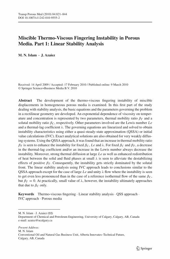
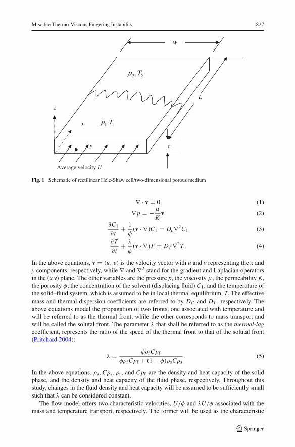
A two-dimensional miscible displacement in a horizontal rectilinear homogeneous mediumof constant porosity φ and permeability K is considered. A fluid of viscosity μ1 and uniformtemperature T1 is injected with a uniform velocity U to displace a second one of viscosityμ2 and uniform temperature T2. Here, the direction of the flow is along the x-axis and they-axis is parallel to the initial plane of the interface (Fig. 1). The length, width, and thicknessof the medium are L, W, and e, respectively.

2.2 Governing Equations

The flow is governed by the equations for the conservation of mass, the conservation ofmomentum in the form of Darcy’s law, and the volume-averaged mass and energy balanceequations.

123


L

e

W

1 1,Tμ

2 2,Tμ

y

x

z

Average velocity U

Fig. 1 Schematic of rectilinear Hele-Shaw cell/two-dimensional porous medium

∇ · v = 0 (1)

∇ p = − μ

Kv (2)

∂C1

∂t+ 1

φ(v · ∇)C1 = Dc∇2C1 (3)

∂T

∂t+ λ

φ(v · ∇)T = DT ∇2T . (4)

In the above equations, v = (u, v) is the velocity vector with u and v representing the x andy components, respectively, while ∇ and ∇2 stand for the gradient and Laplacian operatorsin the (x,y) plane. The other variables are the pressure p, the viscosity μ, the permeability K,the porosity φ, the concentration of the solvent (displacing fluid) C1, and the temperature ofthe solid–fluid system, which is assumed to be in local thermal equilibrium, T. The effectivemass and thermal dispersion coefficients are referred to by DC and DT , respectively. Theabove equations model the propagation of two fronts, one associated with temperature andwill be referred to as the thermal front, while the other corresponds to mass transport andwill be called the solutal front. The parameter λ that shall be referred to as the thermal-lagcoefficient, represents the ratio of the speed of the thermal front to that of the solutal front(Pritchard 2004):

λ = φρf Cpf

φρf Cpf + (1 − φ)ρsCps. (5)

In the above equations, ρs,Cps, ρf , and Cpf are the density and heat capacity of the solidphase, and the density and heat capacity of the fluid phase, respectively. Throughout thisstudy, changes in the fluid density and heat capacity will be assumed to be sufficiently smallsuch that λ can be considered constant.

The flow model offers two characteristic velocities, U/φ and λU/φ associated with themass and temperature transport, respectively. The former will be used as the characteristic

123


velocity in the present study. This choice has been dictated by the fact that U/φ usuallyreferred to as interstitial velocity, is the most commonly used velocity to characterize suchflows. Furthermore, this choice will allow for easy comparison with numerous previousstudies that have focused on the isothermal case. Finally, in the case of a double solutal andthermal fronts, the former will be less diffuse than the latter and is expected to contributemore to the overall instability of the system.

The model equations are expressed in a Lagrangian reference frame moving at the velocityU/φ (Tan and Homsy 1986; Manickam and Homsy 1995; Azaiez and Singh 2002). Further-more, the equations are made dimensionless using DCφ/U,DCφ

2/U 2, and U/φ as thecharacteristic length, time, and velocity. The constant permeability K is incorporated in theexpression of the viscosity by treating μ/K as μ, and ratios of μ shall be referred to as eitherviscosity or mobility ratios. The viscosity and pressure are scaled with μ1 and μ1 DCφ,respectively, and the concentration with that of the displacing fluid C1. Finally, definingthe dimensionless temperature as θ∗ = (T − T2)/(T1 − T2), the following dimensionlessequations are obtained:

∂u∗

∂x∗ + ∂v∗∂y∗ = 0 (6)

∂p∗

∂x∗ = −μ∗(u∗ + 1),∂p∗

∂y∗ = −μ∗v∗

(7)

∂c∗

∂t∗+ u∗ ∂c∗

∂x∗ + v∗ ∂c∗

∂y∗ =(∂2c∗

∂x∗2 + ∂2c∗

∂y∗2

)(8)

∂θ∗

∂t∗+ (λ− 1)

∂θ∗

∂x∗ + λ

(u∗ ∂θ∗

∂x∗ + v∗ ∂θ∗

∂y∗

)= Le

(∂2θ∗

∂x∗2 + ∂2θ∗

∂y∗2

)(9)

Here, Le is the Lewis number, Le = DT /DC = PeC/PeT where PeC and PeT are thesolutal and thermal Peclet numbers. For convenience, in all that follows, the asterisks willbe dropped from all dimensionless variables. In order to complete the model, a form for thedependence of the viscosity on concentration and temperature must be specified. FollowingTan and Homsy (1986) and Pritchard (2004), exponential dependence is adopted:

μ(c, θ) = exp (βc(1 − c)+ βT (1 − θ)) . (10)

In an isothermal miscible displacement, βC corresponds to the natural logarithm of the vis-cosity ratio (μ2/μ1), while in a thermal displacement involving a single fluid βT representsthe natural logarithm of the ratio of the viscosity (μT 2/μT 1) at two different temperatures,and will be referred to as the thermal mobility ratio.

3 Linearized Equations

3.1 Perturbation Equations

The system of Eqs. 6–9 admits the following base state solutions:

u(x, t) = v(x, t) = 0, c(x, t) = 1

2erfc

(x

2√

t

), θ (x, t) = 1

2erfc

(x − (λ− 1)t

2√

Let

)(11)

μ(x, t) = exp(βc(1 − c)+ βT (1 − θ )

), p(x, t) = −

x∫μ(x ′, t)dx ′. (12)

123


In order to conduct a linear stability analysis of the problem, small disturbances noted witha prime are added to the flow at the base state. The linearized equations in terms of theperturbations are:

∂u′

∂x+ ∂v′

∂y= 0 (13)

∂p′

∂x= −μ′ − μu′, ∂p′

∂y= −μv′ (14)

∂c′∂t

+ u′ ∂ c

∂x= ∂2c′∂x2 + ∂2c′

∂y2 (15)

∂θ ′

∂t+ (λ− 1)

∂θ ′

∂x+ λu′ ∂θ

∂x= Le

(∂2θ ′

∂x2 + ∂2θ ′

∂y2

), (16)

where μ′ = c′ ∂μ∂ c + θ ′ ∂μ

∂θ. The linearized equations can be expressed in terms of c′, θ ′ and u′

only. For this purpose, the pressure is eliminated by taking the curl of Darcy’s law (Eq. 14):

μ

(∂v′

∂x− ∂u′

∂y

)− ∂μ′

∂y+ v′ ∂μ

∂x= 0. (17)

The transverse component of the velocity v′ is eliminated by taking the derivative of Eq. 17with respect to y, and using Eq. 13:(

∂2u′

∂x2 + ∂2u′

∂y2

)+ 1

μ

∂μ

∂x

∂u′

∂x+ 1

μ

∂2μ′

∂y2 = 0. (18)

Equations 15, 16, and 18 will then be used in the ensuing linear stability analysis. Since thebase state depends only on the x-coordinate and time, it is possible to use a normal mode anal-ysis of the perturbations where the disturbances are expanded in terms of Fourier componentsin y:

(u′, c′, θ ′) (x, y, t) = (ψ, χ, ϑ) (x, t) eiky (19)

where k is the wavenumber of disturbances in the y direction. Substituting the above expres-sions for the perturbations in Eqs. 15, 16, and 18, along with the use of Eq. 10 one gets:(

∂

∂t− ∂2

∂x2 + k2)χ = − ∂ c

∂xψ (20)

(∂

∂t+ (λ− 1)

∂

∂x− Le

∂2

∂x2 + Le k2)ϑ = −λ∂θ

∂xψ (21)

(∂2

∂x2 − k2 −(βC∂ c

∂x+ βT

∂θ

∂x

)∂

∂x

)ψ = −k2 (βCχ + βTϑ) (22)

− 1

μ

∂μ

∂x= βC

∂ c

∂x+ βT

∂θ

∂x. (23)

Since the base state solutions depend on both time and the spatial component x, it is notpossible a priori to further simplify the above system of partial differential equations. Oneapproach that has been used extensively for isothermal flows is based on the so-called QSSA(Tan and Homsy 1986; Rogerson and Meiburg 1993; Manickam and Homsy 1995; Azaiezand Singh 2002). This approximation is based on the assumption that the growth rate ofperturbations is asymptotically faster than the rate of change of the background state. Assuch, one should be able to determine the most dangerous wavelengths at any point in time

123


at which the base state was “frozen”. As one may have expected, the use of such an approxi-mation raises questions regarding its limitations and conditions of applicability. This has ledto a number of studies that attempted to solve the initial partial differential equations usinga number of techniques including direct solutions using pseudo-spectral methods (Tan andHomsy 1986) and the projection of the disturbances into a suitable space of eigenfunctions(Ben et al. 2002; Pritchard 2004). The solution of the original set of partial differential equa-tions will be referred to as IVC. In this study, we will use both the QSSA and IVC approachesto analyze the flow instability. Since both approaches have advantages and disadvantages,the analysis and comparison of the results of both methods should allow one to determine theextent of applicability of QSSA for studying the instability in double diffusive–convectivethermo-viscous flows.

3.2 Step-Profile Approximation

The limiting case of very short time such that on the timescale considered, diffusion has noeffects on the flow which effectively behaves as immiscible (Rakotomalala et al. 1997), isconsidered first. Under such limiting case, both thermal and solutal fronts are represented bya step-profile; c(x) = θ(x) = 1 − H(x), where H(x) represents the Heaviside step function(Tan and Homsy 1986; Yortsos and Zeybek 1988). In this case, an exponential growth in timefor the perturbations is assumed:

(ψ, χ, ϑ)(x, t) = (ψ, χ, ϑ)(x) exp[γ t]. (24)

With such formulation, the following equations are obtained:

[D2 − l2]χ = −δψ (25)

[LeD2 + (1 − λ)D − h2]ϑ = −λδψ (26)[1

μD(μD) − k2

]ψ = −k2(βCχ + βTϑ) (27)

In the above equation, h2 = γ + Le k2, l2 = γ + k2, D = d/dx , and δ(x) stands forDirac Delta function. Solutions that decay far from the fronts are sought in the form:

χ(x) = A1 · exp(s1lx) x < 0χ(x) = A2 · exp(s2lx) x > 0

(28)

ϑ(x) = B1 · exp(m1x) x < 0ϑ(x) = B2 · exp(m2x) x > 0

(29)

ψ(x) = a A1 · exp(s1lx)+ b1 B1 · exp(m1x)+ C1 · exp(s1kx) x < 0ψ(x) = a A2 · exp(s2lx)+ b2 B2 · exp(m2x)+ C2 · exp(s2kx) x > 0.

(30)

The solutions are valid for x = 0 with s1 = +1 for x < 0 and s2 = −1 for x > 0.The remaining parameters are defined as:

m1 = (λ− 1)+ √(λ− 1)2 + 4Leh2

2Le; m2 = (λ− 1)− √

(λ− 1)2 + 4Leh2

2Le(31)

a = −k2βC

γ(32)

b1 = − k2βT

m21 − k2

; b2 = − k2βT

m22 − k2

. (33)

123


The unknown constants Ai , Bi , and Ci are determined using the following conditions:

χ(0+) = χ(0−) (34)

ϑ(0+) = ϑ(0−) (35)

ψ(0+) = ψ(0−) (36)

Dχ(0+)− Dχ(0−) = −ψ(0) (37)

Le(Dϑ(0+)− Dϑ(0−)) = −λψ(0) (38)

αDψ(0+) = Dψ(0−), (39)

where α = exp(βC + βT ). The above equations are obtained by requiring the perturbationsto be continuous at 0 and by integrating Eqs. 25–27 between 0− and 0+. Equations 34–39lead to a homogenous system of equations for the six unknowns A1, B1,C1, A2, B2, and C2.For non-trivial solutions, the determinant of the corresponding matrix must be zero, whichafter some algebra leads to (see Appendix):

�3m31 +�2m2

1 +�1m1 +�0 = 0 (40)

�3 = 2(1 + α)Le� (41)

�2 = (1 + α)Le�(4k − 3β) (42)

�1 = (1 + α)[Le�(2k2 + β2 − 4kβ)− 2kl(1 + Leβ)βT ] (43)

�0 = (1 + α)[Le�βk(β − k)− 2k2l(1 + Leβ)βT ]+2kl(1 + Leβ)ββT , (44)

where� = 2l −kβC/(l + k), while β = (λ− 1)/Le is always negative. It is worth stressinghere that the above equation is not a cubic equation since the coefficients �i depend on m1

through l:

m1(β − m1) = (1 − Le)k2 − l2

Le(45)

Equation 45 is obtained by taking the product m1 · m2 = m1(β − m1) using Eq. 31 andsimplifying the result using the relationship h2 − l2 = (Le − 1)k2. Equation 45 and thedefinition of l2 will be used to find the growth rate γ once m1 is determined.

3.3 Formulation Based on QSSA

In QSSA, one assumes that the small perturbations change in time much faster than the basestate, allowing treatment of the base state as if it were steady by freezing it at a time to. WhenQSSA is applied, the perturbation functions of Eqs. 19 are defined as:

(ψ, χ, ϑ)(x, t) = (ψ, χ, ϑ)(x, to) exp[γ (to)t], (46)

where γ (t0) is the quasi-static growth rate. Here, it has been assumed that the disturbancesgrow exponentially with time. Substituting the above expression in Eqs. 20–22, and simpli-fying transforms the system of partial differential equations into a corresponding system ofordinary differential equations:

123


(γ (to)− d2

dx2 + k2

)χ = − dc

dx(x, to)ψ (47)

(γ (to)− Le

d2

dx2 + (λ− 1)d

dx+ Lek2

)ϑ = −λdθ

dx(x, to)ψ (48)

[d2

dx2 − k2 −{βC

dc

dx(x, to)+ βT

dθ

dx(x, to)

}d

dx

]ψ = −k2(βCχ + βTϑ).

(49)

The above system of equations represents an eigenvalue differential problem with the bound-ary conditions (ψ, χ, ϑ) → (0, 0, 0) as x → ±∞. The quasi-static growth rate representedby the eigenvalue γ (t0) is a function of the parameter t0, and depends on the values of thewavenumber k, the two viscosity parameters βC and βT , the thermal-lag coefficient λ andthe Lewis number Le. Thus, through finite difference discretization of Eqs. 47–49 one canobtain the eigenvalue at any time t0. A non-uniform geometric grid is used which is veryfine near the origin where the concentration and temperature gradients are large, and spacingincreases geometrically with the distance from the origin. All three eigenfunctions (ψ, χ, ϑ)are discretized using this technique, and the computation domain is chosen wide enough tocapture all the eigen-solutions. Finite difference discretization of the above equations resultsin the forms:

(A − γ I)χ = Cψ (50)

(B − γ I)ϑ = Tψ (51)

Kψ = Lχ + Mϑ, (52)

where A, B, and K are the tri-diagonal matrices, C, T, L, and M are diagonal matrices andI is the identity matrix. The above set of equations is rearranged to obtain the appropriateeigenvalue problem:

[A − CK−1L −CK−1M−TK−1L B − TK−1M

] [χ

ϑ

]= γ

[χ

ϑ

](53)

3.4 Formulation Based on IVC

This approach consists in solving the initial partial differential equations without invokingthe QSSA and determining the growth rate from the solution (Tan and Homsy 1986). Thus,the set of coupled partial differential Eqs. 20–22 are solved directly and the growth rates ofindividual perturbations are determined using the following expression:

η f = 1

�tlog

(‖ f ‖t+�t

‖ f ‖t

), (54)

where f may representψ, χ , orϑ . Determination of the growth rates of the perturbations usingthe initial value calculation introduced an additional feature—it recognized the differenceof the growth rates for velocity, concentration, and temperature perturbations. The partialdifferential equations are solved with decaying boundary conditions and the following initialconditions:

χ(x, to) = δ ∗ rand(x) (55)

ϑ(x, to) = δ ∗ rand(x) (56)

123


The perturbation terms (Eqs. 55 and 56) consist of a random noise obtained from a randomnumber generator between −1 and 1, and a parameter δ that determines the amplitude ofthe perturbation. In order to capture the growth dynamics of the perturbations at very earlytime, t0 is set to 10−24 and perturbations of very small amplitude are introduced by settingδ = 10−8.

Since the perturbations are required to decay far from the interface, periodic boundaryconditions can be used. Such conditions allow using the highly accurate spectral methods. Inthis study, the Hartley transform based pseudo-spectral method (Canuto et al. 1987; Bracewell2000) is used. With this transform the flow variables are expanded in the one-dimensionalHartley series, which for an arbitrary function g(x, t) has the form:

H [g(x, t)] = 1√Nx

Nx∑i=1

g(xi , t)cas(kx xi ) (57)

where xi = 2π iNx, cas(u) = cos(u) + sin(u), kx is the discrete wavenumber, and Nx is the

number of spectral modes in the x direction. The most prominent feature of using such trans-formation is that it allows recasting the partial differential equations in space and time forthe concentration and temperature into ordinary differential equations in time with algebraicconstraints. The implementation of the numerical method is similar to the work of and Singhand Azaiez (2001) which the readers are referred to for details.

Once the partial differential equations are integrated up to a certain time t for a particularwavenumber k, the growth rates ηψ, ηχ and ηϑ are calculated using Eq. 54. The largest ofthe growth rates ηψ, , ηχ , and ηϑ is chosen to represent the growth rate of the instability.Repeating the calculations for varying k allows one to obtain a full instability characteristicscurve. All simulations were run up to a time t = 10 around which the growth rates of theperturbations were found to reach a plateau.

4 Results

In linear stability analysis, the model equations describing a dynamic system are first linear-ized and then solved to determine the growth rates of the associated wavenumbers—definingthe perturbations introduced into the system. This way, it is possible to set criteria basedon which the stability of a dynamic system can be determined and possibly explained. Inwhat follows, determination of the initial growth rates for unstable wavenumbers will bediscussed first. Later, results of numerical solutions of the eigenvalue problem as well asIVC formulation will be presented.

4.1 Analytical Solution for Step Base State Profiles

Before discussing the results, the case of an isothermal flow (βT = 0) is examined first.In this special case, Eq. 40 reduces to:

(1 + α)Le�(m1 + k)(m1 − β + k)(2m1 − β) = 0. (58)

The solution of the above equation is obtained by requiring� = 0, which leads to the expres-sion of growth rate obtained by Tan and Homsy (1986), which from now on, will be referredto as TH86. The case of a pure thermal flow displacement will be now examined.

123


4.1.1 Flow displacement with a single thermal front

The special case of a thermal flow (βC = 0, Le = 1) involving the same fluid, but at twodifferent temperatures is considered here. The condition Le = 1 is simply implying that, inthis case, the thermal diffusivity is used instead of the mass diffusivity in the scaling of theoriginal equations. In this case, Eq. 40 reduces to:

2m31 + (4k − 3β)m2

1 + [2k2 + β2 − 4kβ − k(1 + β)βT ]m1 + kβ(β − k)− k2(1 + β)βT

+k(1 + β)ββT

1 + α= 0. (59)

The above equation, expressed in a reference frame moving with the superficial velocity isdifferent from that for an isothermal flow. It is, however, easy to see that expected resultsfor an isothermal flow with βT replacing βC are readily obtained when a reference framemoving at the thermal front velocity is used (β = 0). Equation 59 where the thermal frontlags behind the perturbation (β = 0) will be now examined.

4.1.1.1 Long Wave Expansion and Cut-Off Wavenumbers A long wave expansion of m1

using Eq. 59 leads to:

m1 = −[1 + (1 + β)

β

βT

1 + α]k + o(k) (60)

γ = β[1 + (1 + β)

β

βT

1 + α]k + o(k). (61)

The above expression indicates that for any logarithmic thermal mobility ratio βT , thereis a critical lag coefficient βC1 = −βT

1+βT +eβT, such that the flow is unstable to long wave

disturbances only if β > βC1. Furthermore, since f (βT ) = βT

1+eβTreaches a maximum

of fmax = 0.278 at βT c = 1.278, the flow will be unstable to long wave disturbances ifβ > −0.218 or λ > 0.782.

In order to determine whether the flow is stable or unstable over the whole spectrum ofwavenumbers, the wavenumbers at which the growth rate is zero are examined. Such growthrates are given by:

k2(2k2 + 1k + 0) = 0 (62)

2 = 4[(1 + β)βT (α2 − 1)− β(1 + α)2] (63)

1 = −(1 + β)2β2T (α

2 − 1) (64)

0 = β(βT + α + 1)(αβT − α − 1)(β − βC1)(β − βC2), (65)

where βC2 = −βT eβT

βT eβT −eβT −1. It is easy to see that one recovers the cut-off wavenumber βT /4

in the case β = 0 (TH86). Furthermore, one should note that 2 is always positive while1 is always negative. One can show that if β > βC1, 0 is negative and Eq. 62 will have tworeal roots (one negative and one positive), the latter corresponding to the cut-off wavenum-ber of the unstable flow. On the other hand, if β < βC1 then 0 is positive and Eq. 62 mayeither have two real positive roots or two complex roots. In the latter case, the flow will bestable for all wavenumber, while for the former it will be unstable for a finite spectrum thatdoes not include long waves.

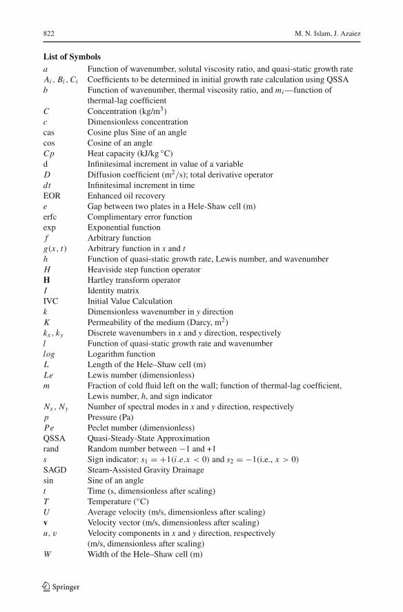
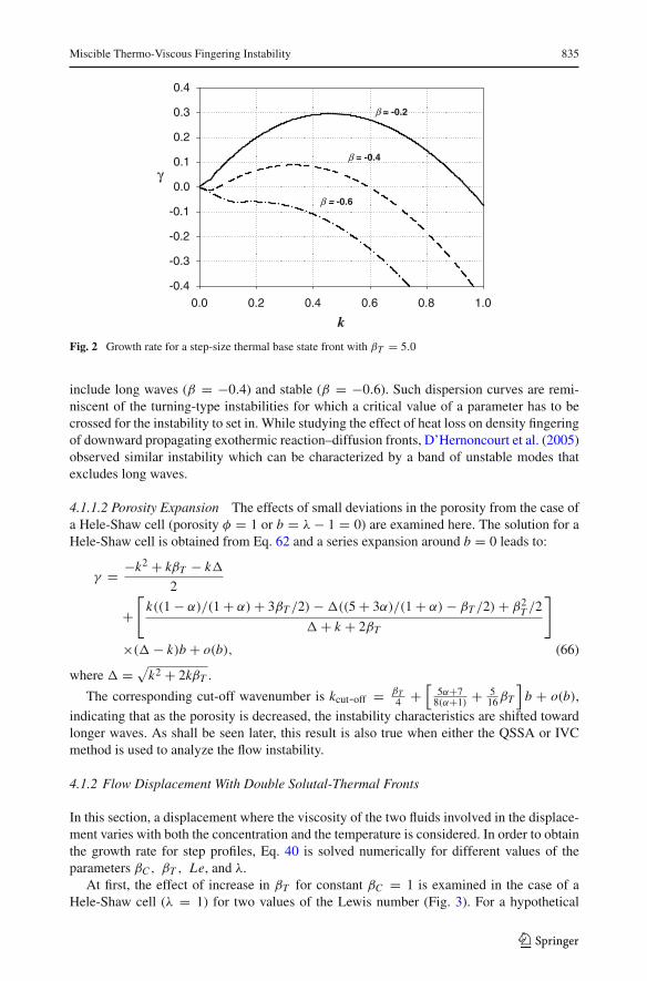
Figure 2 depicts instability characteristics obtained by solving numerically Eq. 59 forβT = 5 and various values of β. The three curves illustrate the three possibilities discussedearlier where the flow may be unstable (β = −0.2), unstable for a spectrum that does not

123


β = -0.6

k0.0 0.2 0.4 0.6 0.8 1.0

γ

-0.4

-0.3

-0.2

-0.1

0.0

0.1

0.2

0.3

0.4

β = -0.4

β = -0.2

Fig. 2 Growth rate for a step-size thermal base state front with βT = 5.0

include long waves (β = −0.4) and stable (β = −0.6). Such dispersion curves are remi-niscent of the turning-type instabilities for which a critical value of a parameter has to becrossed for the instability to set in. While studying the effect of heat loss on density fingeringof downward propagating exothermic reaction–diffusion fronts, D’Hernoncourt et al. (2005)observed similar instability which can be characterized by a band of unstable modes thatexcludes long waves.

4.1.1.2 Porosity Expansion The effects of small deviations in the porosity from the case ofa Hele-Shaw cell (porosity φ = 1 or b = λ− 1 = 0) are examined here. The solution for aHele-Shaw cell is obtained from Eq. 62 and a series expansion around b = 0 leads to:

γ = −k2 + kβT − k�

2

+[

k((1 − α)/(1 + α)+ 3βT /2)−�((5 + 3α)/(1 + α)− βT /2)+ β2T /2

�+ k + 2βT

]

×(�− k)b + o(b), (66)

where � = √k2 + 2kβT .

The corresponding cut-off wavenumber is kcut-off = βT4 +

[5α+7

8(α+1) + 516βT

]b + o(b),

indicating that as the porosity is decreased, the instability characteristics are shifted towardlonger waves. As shall be seen later, this result is also true when either the QSSA or IVCmethod is used to analyze the flow instability.

4.1.2 Flow Displacement With Double Solutal-Thermal Fronts

In this section, a displacement where the viscosity of the two fluids involved in the displace-ment varies with both the concentration and the temperature is considered. In order to obtainthe growth rate for step profiles, Eq. 40 is solved numerically for different values of theparameters βC , βT , Le, and λ.

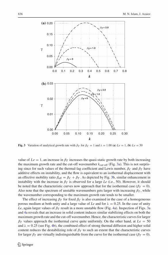
At first, the effect of increase in βT for constant βC = 1 is examined in the case of aHele-Shaw cell (λ = 1) for two values of the Lewis number (Fig. 3). For a hypothetical

123


βT = 0

k

0.0 0.1 0.2 0.3 0.4 0.5 0.6 0.7 0.8

γ

0.00

0.05

0.10

0.15

0.20

βT = 1.0

βT = 2.0

(a)

βT = 0

k

0.00 0.05 0.10 0.15 0.20 0.25 0.30

γ

0.00

0.01

0.02

0.03

βT = 1.0

βT = 2.0

(b)

Fig. 3 Variation of analytical growth rate with βT for βC = 1 and λ = 1.00 (a) Le = 1, (b) Le = 50

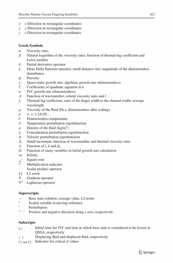
value of Le = 1, an increase in βT increases the quasi-static growth rate by both increasingthe maximum growth rate and the cut-off wavenumber kcut-off (Fig. 3a). This is not surpris-ing since for such values of the thermal-lag coefficient and Lewis number, βC and βT haveadditive effects on instability, and the flow is equivalent to an isothermal displacement withan effective mobility ratio βeff = βC + βT . As depicted by Fig. 3b, similar enhancement ininstability with the increase in βT is observed for a large Le (i.e., 50). However, it shouldbe noted that the characteristic curves now approach that for the isothermal case (βT = 0).Also note that the spectrum of unstable wavenumbers gets larger with increasing βT , whilethe wavenumber corresponding to the maximum growth rate tends to be smaller.

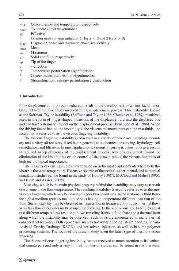
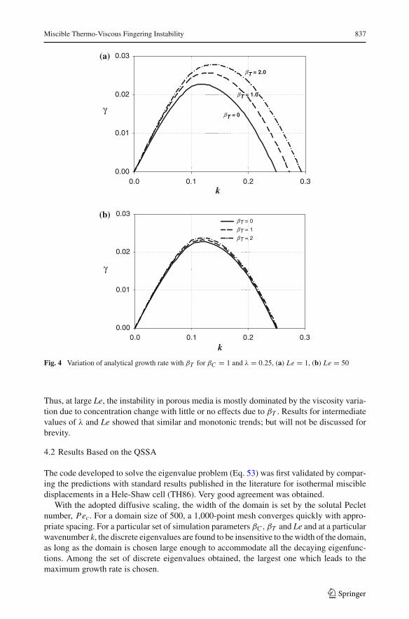
The effect of increasing βT for fixed βC is also examined in the case of a homogeneousporous medium at both unity and a large value of Le and for λ = 0.25. In the case of unityLe, again larger values of βT result in a more unstable flow (Fig. 4a). Inspection of Figs. 3aand 4a reveals that an increase in solid content induces similar stabilizing effects on both themaximum growth rate and the cut-off wavenumber. Hence, the characteristic curves for largerβT values approach the isothermal curve quite uniformly. On the other hand, at Le = 50and λ = 0.25 (see Fig. 4b), the combined effect of strong thermal diffusion and higher solidcontent reduces the destabilizing role of βT to such an extent that the characteristic curvesfor larger βT are virtually indistinguishable from the curve for the isothermal case (βT = 0).

123


βT = 0

k0.0 0.1 0.2 0.3

γ

0.00

0.01

0.02

0.03

βT = 1.0

βT = 2.0

(a)

k0.0 0.1 0.2 0.3

γ

0.00

0.01

0.02

0.03βT = 0

βT = 1

βT = 2

(b)

Fig. 4 Variation of analytical growth rate with βT for βC = 1 and λ = 0.25, (a) Le = 1, (b) Le = 50

Thus, at large Le, the instability in porous media is mostly dominated by the viscosity varia-tion due to concentration change with little or no effects due to βT . Results for intermediatevalues of λ and Le showed that similar and monotonic trends; but will not be discussed forbrevity.

4.2 Results Based on the QSSA

The code developed to solve the eigenvalue problem (Eq. 53) was first validated by compar-ing the predictions with standard results published in the literature for isothermal miscibledisplacements in a Hele-Shaw cell (TH86). Very good agreement was obtained.

With the adopted diffusive scaling, the width of the domain is set by the solutal Pecletnumber, Pec. For a domain size of 500, a 1,000-point mesh converges quickly with appro-priate spacing. For a particular set of simulation parameters βC , βT and Le and at a particularwavenumber k, the discrete eigenvalues are found to be insensitive to the width of the domain,as long as the domain is chosen large enough to accommodate all the decaying eigenfunc-tions. Among the set of discrete eigenvalues obtained, the largest one which leads to themaximum growth rate is chosen.

123


βT = 0

k

0.0 0.1 0.2 0.3 0.4

γ

0.00

0.02

0.04

0.06

0.08

βT = 1.0

βT = 2.0

(a)

βT = 0

k0.00 0.05 0.10 0.15 0.20

γ

0.000

0.005

0.010

0.015

0.020

βT = 1.0βT = 2.0

(b)

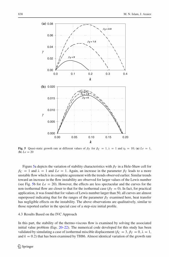
Fig. 5 Quasi-static growth rate at different values of βT for βC = 1, λ = 1 and t0 = 10; (a) Le = 1,(b) Le = 20

Figure 5a depicts the variation of stability characteristics with βT in a Hele-Shaw cell forβC = 1 and λ = 1 and Le = 1. Again, an increase in the parameter βT leads to a moreunstable flow which is in complete agreement with the trends observed earlier. Similar trendstoward an increase in the flow instability are observed for larger values of the Lewis number(see Fig. 5b for Le = 20). However, the effects are less spectacular and the curves for thenon-isothermal flow are closer to that for the isothermal case (βT = 0). In fact, for practicalapplication, it was found that for values of Lewis number larger than 50, all curves are almostsuperposed indicating that for the ranges of the parameter βT examined here, heat transferhas negligible effects on the instability. The above observations are qualitatively, similar tothose reported earlier in the special case of a step-size initial profile.

4.3 Results Based on the IVC Approach

In this part, the stability of the thermo-viscous flow is examined by solving the associatedinitial value problem (Eqs. 20–22). The numerical code developed for this study has beenvalidated by simulating a case of isothermal miscible displacement (βC = 3, βT = 0, λ = 1,and k = 0.2) that has been examined by TH86. Almost identical variation of the growth rate

123


k

0.00 0.05 0.10 0.15 0.20

ηψ

0.000

0.005

0.010

0.015

0.020 βT = 0

βT = 1

βT = 1.5

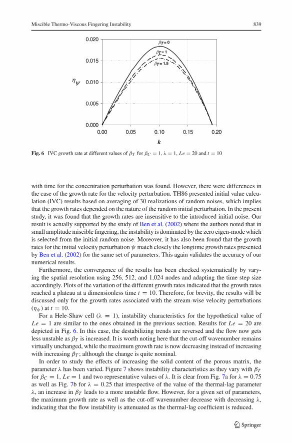
Fig. 6 IVC growth rate at different values of βT for βC = 1, λ = 1, Le = 20 and t = 10

with time for the concentration perturbation was found. However, there were differences inthe case of the growth rate for the velocity perturbation. TH86 presented initial value calcu-lation (IVC) results based on averaging of 30 realizations of random noises, which impliesthat the growth rates depended on the nature of the random initial perturbation. In the presentstudy, it was found that the growth rates are insensitive to the introduced initial noise. Ourresult is actually supported by the study of Ben et al. (2002) where the authors noted that insmall amplitude miscible fingering, the instability is dominated by the zero eigen-mode whichis selected from the initial random noise. Moreover, it has also been found that the growthrates for the initial velocity perturbationψ match closely the longtime growth rates presentedby Ben et al. (2002) for the same set of parameters. This again validates the accuracy of ournumerical results.

Furthermore, the convergence of the results has been checked systematically by vary-ing the spatial resolution using 256, 512, and 1,024 nodes and adapting the time step sizeaccordingly. Plots of the variation of the different growth rates indicated that the growth ratesreached a plateau at a dimensionless time t = 10. Therefore, for brevity, the results will bediscussed only for the growth rates associated with the stream-wise velocity perturbations(ηψ ) at t = 10.

For a Hele-Shaw cell (λ = 1), instability characteristics for the hypothetical value ofLe = 1 are similar to the ones obtained in the previous section. Results for Le = 20 aredepicted in Fig. 6. In this case, the destabilizing trends are reversed and the flow now getsless unstable as βT is increased. It is worth noting here that the cut-off wavenumber remainsvirtually unchanged, while the maximum growth rate is now decreasing instead of increasingwith increasing βT ; although the change is quite nominal.

In order to study the effects of increasing the solid content of the porous matrix, theparameter λ has been varied. Figure 7 shows instability characteristics as they vary with βT

for βC = 1, Le = 1 and two representative values of λ. It is clear from Fig. 7a for λ = 0.75as well as Fig. 7b for λ = 0.25 that irrespective of the value of the thermal-lag parameterλ, an increase in βT leads to a more unstable flow. However, for a given set of parameters,the maximum growth rate as well as the cut-off wavenumber decrease with decreasing λ,indicating that the flow instability is attenuated as the thermal-lag coefficient is reduced.

123


k

0.00 0.05 0.10 0.15 0.20 0.25 0.30 0.35

ηψ

0.00

0.01

0.02

0.03

0.04

0.05

0.06

0.07

βT

= 0

βT

= 1

βT = 2

(a)

k

0.00 0.05 0.10 0.15 0.20 0.25

ηψ

0.00

0.01

0.02

0.03

βT = 0

βT = 1

βT = 2(b)

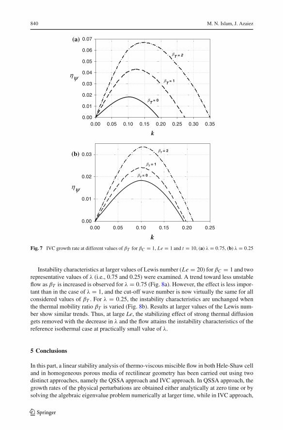
Fig. 7 IVC growth rate at different values of βT for βC = 1, Le = 1 and t = 10, (a) λ = 0.75, (b) λ = 0.25

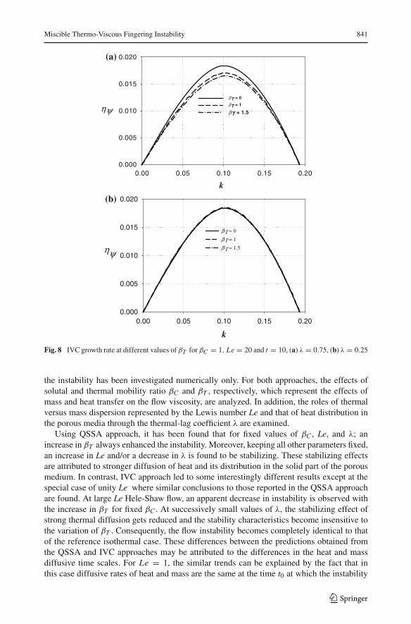
Instability characteristics at larger values of Lewis number (Le = 20) for βC = 1 and tworepresentative values of λ (i.e., 0.75 and 0.25) were examined. A trend toward less unstableflow as βT is increased is observed for λ = 0.75 (Fig. 8a). However, the effect is less impor-tant than in the case of λ = 1, and the cut-off wave number is now virtually the same for allconsidered values of βT . For λ = 0.25, the instability characteristics are unchanged whenthe thermal mobility ratio βT is varied (Fig. 8b). Results at larger values of the Lewis num-ber show similar trends. Thus, at large Le, the stabilizing effect of strong thermal diffusiongets removed with the decrease in λ and the flow attains the instability characteristics of thereference isothermal case at practically small value of λ.

5 Conclusions

In this part, a linear stability analysis of thermo-viscous miscible flow in both Hele-Shaw celland in homogeneous porous media of rectilinear geometry has been carried out using twodistinct approaches, namely the QSSA approach and IVC approach. In QSSA approach, thegrowth rates of the physical perturbations are obtained either analytically at zero time or bysolving the algebraic eigenvalue problem numerically at larger time, while in IVC approach,

123


k

0.00 0.05 0.10 0.15 0.200.000

0.005

0.010

0.015

0.020

βT = 0

βT = 1

βT = 1.5ηψ

(a)

k

0.00 0.05 0.10 0.15 0.20

ηψ

0.000

0.005

0.010

0.015

0.020

βΤ = 0βΤ = 1βΤ = 1.5

(b)

Fig. 8 IVC growth rate at different values of βT for βC = 1, Le = 20 and t = 10, (a) λ = 0.75, (b) λ = 0.25

the instability has been investigated numerically only. For both approaches, the effects ofsolutal and thermal mobility ratio βC and βT , respectively, which represent the effects ofmass and heat transfer on the flow viscosity, are analyzed. In addition, the roles of thermalversus mass dispersion represented by the Lewis number Le and that of heat distribution inthe porous media through the thermal-lag coefficient λ are examined.

Using QSSA approach, it has been found that for fixed values of βC , Le, and λ; anincrease in βT always enhanced the instability. Moreover, keeping all other parameters fixed,an increase in Le and/or a decrease in λ is found to be stabilizing. These stabilizing effectsare attributed to stronger diffusion of heat and its distribution in the solid part of the porousmedium. In contrast, IVC approach led to some interestingly different results except at thespecial case of unity Le where similar conclusions to those reported in the QSSA approachare found. At large Le Hele-Shaw flow, an apparent decrease in instability is observed withthe increase in βT for fixed βC . At successively small values of λ, the stabilizing effect ofstrong thermal diffusion gets reduced and the stability characteristics become insensitive tothe variation of βT . Consequently, the flow instability becomes completely identical to thatof the reference isothermal case. These differences between the predictions obtained fromthe QSSA and IVC approaches may be attributed to the differences in the heat and massdiffusive time scales. For Le = 1, the similar trends can be explained by the fact that inthis case diffusive rates of heat and mass are the same at the time t0 at which the instability

123


is determined. However, for large Le, heat diffuses faster than mass and the assumption ofa quasi-steady base state may be applicable to one, but not the other. Hence, the failureof the QSSA approach to identify the strong stabilizing effects at large Le which can evenmake the flow less unstable than the reference isothermal case. Moreover, it will be shown inthe next part dealing with full nonlinear simulations that the conclusions obtained from theIVC approach are in concordance with those attained from nonlinear evolution of fingers.Thus, it can be concluded that the IVC approach captures better the inherent features of thethermo-viscous flow instability.

In practical terms, the results of the analysis indicate that heat effects act toward makingthe displacement less unstable in the sense that initial disturbances will have weaker growthrates and, hence, one should expect slower growth of instabilities. However, the spectrum ofunstable wave-numbers is virtually unchanged by thermal effects implying that even thoughweaker, the initial disturbances that develop in the flow will have the same wavelengths.Finally, it should be stressed that these trends will be less noticeable if the rate of heat lossfrom the fluids to the surrounding medium become important. In such a case, thermal effectswill cease to play a role in the displacement process which becomes simply dominated bysolutal effects.

Acknowledgments This study was supported by the Natural Science and Engineering Research Council ofCanada (NSERC) and the Alberta Ingenuity Centre for In-Situ Energy (AICISE). The authors also acknowl-edge the use of the computing resources of the West-Grid cluster.

Appendix

Applying the decay conditions at x → ±∞, the general solution for Eqs. 26 and 27 is:

ψ = A1 exp(m1x)+ B1 exp(kx) x < 0ψ = A2 exp(m2x)+ B2 exp(−kx) x > 0

}. (A1)

The continuity of u velocity at x = 0 yields:

ψ(0−) = ψ(0+). (A2)

While the jump in the normal stress at x = 0 results in:

μ(0−) ∂ψ∂x(0−) = μ(0+) ∂ψ

∂x(0+)

or,dψ

dx(0−) = α

dψ

dx(0+) (A3)

where α represents the viscosity ratio [α = μ(0+)/μ(0−) = exp(βT )].The continuity of temperature at x = 0 yields:

θ(0−) = θ(0+). (A4)

Using Eqs. A2 and A4, Eq. 27 can be expressed in terms of the velocity disturbance eigen-function as:

d2ψ

dx2 (0−) = d2ψ

dx2 (0+) (A5)

123


Furthermore, integrating combined equation resulting from Eqs. 26 and 27 from 0− to 0+leads to:

∫ 0+

0−

(d2

dx2 − (λ− 1)d

dx− l2

) (d2

dx2 + βT δ(x)d

dx− k2

)ψdx

= λβT k2∫ 0+

0−δ(x)ψdx . (A6)

Satisfying Eqs. (A2–A5) in conjunction with the general form of the solution (Eq. A1) leadsto the following four equations relating the constant terms A1,B1,A2, and B2:

A1 + B1 − A2 − B2 = 0 (A7)

m1 A1 + k B1 − αm2 A2 + αk B2 = 0 (A8)

m21 A1 + k2 B1 − m2

2 A2 − k2 B2 = 0 (A9)

(m3

1 − (l2 + k2)m1 + βT2 (m1l2 + λk2)

)A1 +

(−l2k + βT

2 (l2k + λk2)

)B1

+(−m3

2 + (l2 + k2)m2 + βT2 (m2l2 + λk2)

)A2 +

(−l2k + βT

2 (−l2k + λk2))

B2 = 0.

(A10)

A non-zero solution is obtained if and only if the determinant of the above matrix is zero:

∣∣∣∣∣∣∣∣∣∣∣

1m1

m21

m31 − (l2 + k2)m1 + βT

2 (m1l2 + λk2)

0m1 − k

m21 − k2

m31 − (l2 + k2)m1 + βT

2 (m1l2 + λk2)

+l2k − βT2 (l

2k + λk2)

0m1 − αm2

m21 − m2

2

m31 − (l2 + k2)m1 + βT

2 (m1l2 + λk2)

−m32 + (l2 + k2)m2 + βT

2 (m2l2 + λk2)

0(1 + α)k

0−l2k + βT

2 (l2k + λk2)

−l2k + βT2 (−l2k + λk2)

∣∣∣∣∣∣∣∣∣∣∣= 0. (A11)

Upon simplification, the determinant of the above matrix will allow to determine the initialgrowth rate of an infinitesimal perturbation. In the following steps, two important relationsbetween the roots m1 and m2 are used

m1m2 = −l2 (A12)

m1 + m2 = λ− 1 = b. (A13)

This leads to:

k(m1 − k)(m1 − b − k)∣∣∣∣∣∣1 (1 + α) (1 + α)

m1 + k b 0m1b + m1k − βT m1(b−m1)

2 2m1k + b2 − bk 2m1b − 2m21 + λβT k

∣∣∣∣∣∣ = 0. (A14)

123


References

Azaiez, J., Singh, B.: Stability of miscible displacements of shear thinning fluids in a Hele-Shaw cell. Phys.Fluids 14, 1557–1571 (2002)

Ben, Y., Demekhin, E.A., Chang, H.-C.: A spectral theory for small-amplitude miscible fingering. Phys.Fluids 14, 999–1010 (2002)

Bensimon, D., Kadanoff, L.P., Liang, S., Shraiman, B.I., Tang, C.: Viscous flows in two dimensions. Rev.Mod. Phys. 58, 977–999 (1986)

Bracewell, R.N.: The Fourier Transform and its Applications. McGraw Hill, New York (2000)Canuto, C., Hussaini, M.Y., Quarteroni, A., Zang, T.A.: Spectral Methods in Fluid Dynamic. Springer,

New York (1987)Chuoke R.L., van Meurs P., Van der Poel, C.: The instability of slow, immiscible, viscous liquid-liquid dis-

placements in permeable media, Trans. AIME 216, 188–194 (1959)D’Hernoncourt, J., Kalliadasis, S., De Wit, A.: Fingering of exothermic reaction-diffusion fronts in Hele-Shaw

cells with conducting walls. J. Chem. Phys. 123, 234503(1–9) (2005)Holloway, K.E., de Bruyn, J.: Viscous fingering with a single fluid. Can. J. Phys. 83, 551–564 (2005)Homsy, G.M.: Viscous fingering in porous media. Ann. Rev. Fluid Mech. 19, 271–311 (1987)Islam, M.N., Azaiez, J.: Fully implicit finite difference pseudo-spectral method for simulating high mobility-

ratio miscible displacements. Int. J. Numer. Methods Fluids 47, 161–183 (2005)Kong, X., Haghighi, M., Yortsos, Y.C.: Visualization of steam displacement of heavy oils in a Hele-Shaw

cell. Fuel 71, 1465–1471 (1992)Kuang, J., Maxworthy, T.: The effect of thermal diffusion on miscible viscous displacement in a capillary

tube. Phys. Fluids A 15, 1340–1343 (2003)Manickam, O., Homsy, G.M.: Fingering instabilities in vertical miscible displacement flows in porous media.

J. Fluid Mech. 288, 75–102 (1995)McCloud, K.V., Maher, J.V.: Experimental perturbations to Saffman-Taylor flow. Phys. Rep. 260,

139–185 (1995)Pritchard, D.: The instability of thermal and fluid fronts during radial injection in a porous medium. J. Fluid

Mech. 508, 133–163 (2004)Rakotomalala, N., Salin, D., Watzky, P.: Miscible displacement between two parallel plates: BGK lattice gas

simulations. J. Fluid Mech. 338, 277–297 (1997)Rogerson, A., Meiburg, E.: Numerical simulation of miscible displacement processes in porous media flows

under gravity. Phys. Fluids A 5, 2644–2660 (1993)Saffman, P.G., Taylor, G.: The penetration of a fluid into a porous medium or Hele-Shaw cell containing a

more viscous liquid. Proc. R. Soc. Lond. A 245, 312–329 (1958)Saghir, M.Z., Chaalal, O., Islam, M.R.: Numerical and experimental modeling of viscous fingering during

liquid-liquid miscible displacement. J. Pet. Sci. Eng. 26, 253–262 (2000)Sasaki, K., Akibayashi, S., Yazawa, N., Kaneko, F.: Microscopic visualization with high resolution optical-fiber

scope at steam chamber interface on initial stage of SAGD process. SPE paper no. 75241 (2002)Sheorey, T., Muralidhar, K., Mukherjee, P.P.: Numerical experiments in the simulation of enhanced oil recovery

from a porous formation. Int. J. Therm. Sci. 40, 981–997 (2001)Singh, B., Azaiez, J.: Numerical simulation of viscous fingering of shear-thinning fluids. Can. J. Chem. Eng.

79, 961–967 (2001)Tan, C.T., Homsy, G.M.: Stability of miscible displacements in porous media: rectilinear flow. Phys.

Fluids 29, 3549–3556 (1986)Yortsos, Y.C., Zeybek, M.: Dispersion driven instability in miscible displacement in porous media. Phys.

Fluids 31, 3511–3518 (1988)

123

Documents

Miscible Thermo-Viscous Fingering Instability in Porous